Improved models for long-term prediction of tropospheric...

IEEE TRANSACTIONS ON ANTENNAS AND PROPAGATION, VOL. 47, NO. 2, FEBRUARY 1999 249

Improved Models for Long-Term Prediction ofTropospheric Scintillation on Slant Paths

Max M. J. L. van de Kamp,Student Member, IEEE, Jouni K. Tervonen,Erkki T. Salonen, and J. Pedro V. Poiares Baptista,Member, IEEE

Abstract—The prediction models for tropospheric scintillationon earth-satellite paths from Karasawa, Yamada, and Allnuttand ITU-R are compared with measurement results from satellitelinks in Europe, the United States, and Japan at frequencies from7 to 30 GHz and elevation angles of 3 to 33�. The existing pre-diction models relate the long-term average scintillation intensityto the wet term of refractivity at ground level. The comparisonshows that the seasonal variation of scintillation intensity is wellpredicted by this relation, but for the annual average someadditional meteorological information is needed. A much betteragreement with measurement results is found when a parameterrepresenting the average water content of heavy clouds is incor-porated. This confirms the assumption that scintillation is, at leastpartly, associated with turbulence inside clouds. The asymmetrybetween the distributions of signal fade and enhancement can alsobe explained by turbulence inside clouds. The asymmetry dependson the intensity of the scintillation, which is consistent with thetheory assuming a thin layer of cloudy turbulence. A new modelbased on this theory predicts the distributions of signal fade andenhancement significantly better.

Index Terms—Cloud water content, cumulus clouds, low-fademargin, meteorology, propagation, radio-wave propagation, satel-lite communication, tropospheric scintillation, tropospheric tur-bulence.

I. INTRODUCTION

I NCREASING demand for -band (14/12/11 GHz) re-sources will require the provision of additional spectrum in

higher bands. Some systems are already designed to operatein the 30/20 GHz band ( band) and it is probable thatserious consideration will be given soon to utilizing the 50/40GHz band ( band). - and -band applications willbe aimed at very small aperture terminal (VSAT) serviceswith low-fade margins. Thus, there is a pressing need toquantify attenuation phenomena in the relatively low-fademargin range. Furthermore, new satellite constellations usinglow earth orbits such as Teledesic and Iridium are plannedwith -band links, which may have to operate occasionally

Manuscript received September 30, 1997; revised June 5, 1998. This workwas supported in part by Helsinki University of Technology, Helsinki, Finland,under ESA/ESTEC Contract 10827/94/NL/NB(SC).

M. M. J. L. van de Kamp is with the Eindhoven University of Technology,Radiocommunications Group, 5600 MB Eindhoven, The Netherlands.

J. K. Tervonen is with the Helsinki University of Technology, RadioLaboratory, 02015 HUT, Helsinki, Finland.

E. T. Salonen is with the University of Oulu, Telecommunications Labora-tory, 90571 Oulu, Finland.

J. P. V. Poiares Baptista is with the ESA/ESTEC, XEP, 2200 AG Noord-wijk, The Netherlands.

Publisher Item Identifier S 0018-926X(99)03733-3.

at low elevation angles, where tropospheric scintillation maybe a significant impairment.

Tropospheric scintillation is a rapid fluctuation of signalamplitude and phase due to turbulent irregularities in temper-ature, humidity, and pressure, which translate into small-scalevariations in refractive index. In the microwave region, wherethe humidity fluctuations are important, the result is randomdegradation and enhancement in signal amplitude and phasereceived on a satellite–earth link, as well as a degradation inperformance of large antennas.

In general, the impact of rain attenuation on communicationsignals is predominant at frequencies10 GHz. Scintillation,however, becomes important for low-fade margin systemsoperating at frequencies10 GHz and at low elevation angles( 15 ) since on these, scintillation may cause as muchattenuation as rain, especially for time percentages larger than1%. Knowledge of the dynamic characteristics of scintillationis also important for the design of up-link power control andantenna tracking systems.

Early models for the prediction of scintillation effects relatethe long-term scintillation intensity to the wet term of therefractivity at ground level, which is a function of temper-ature and humidity. When these models were formulated, fewmeasurement results were available to verify the predictions.A number of new measurement results are now available, andthe models are tested here using these results from severaldifferent sites in different continents.

II. CURRENT PREDICTION MODELS

A. Long-Term Correlation with Meteorology

Karasawaet al. [1] presented a prediction method for thecalculation of the standard deviationof signal fluctuationsdue to scintillation, based on measurements made during 1983at Yamaguchi, Japan, at an elevation angle of 6.5, frequenciesof 11.5 and 14.23 GHz, and an antenna diameter of 7.6 m. Forthe elevation angle dependence, they used long-term data fromthe same site at elevation angles of 4and 9 . Using these data,they derived the following prediction formula:

dB (1)

where

ppm (2)

0018–926X/99$10.00 1999 IEEE

250 IEEE TRANSACTIONS ON ANTENNAS AND PROPAGATION, VOL. 47, NO. 2, FEBRUARY 1999

and is the predicted signal standard deviation or “scintil-lation intensity,” is the frequency in GHz, is the apparentelevation angle, is the wet term of the refractivity atground level, is the relative humidity in percent, andis thetemperature in degrees centigrade. These meteorological inputparameters should be averaged over a period in the order ofa month so the model does not predict short-term scintillationvariations with daily weather changes. is an antennaaveraging function, given by Crane and Blood [2], and isthe effective antenna diameter given by with asthe geometrical antenna diameter andthe antenna apertureefficiency. The antenna averaging function also depends on theelevation angle and the height of the turbulence, assumed byKarasawaet al. to be 2000 m. If , in (1) should

be replaced by , where is theheight of the turbulence and is the effective earth radius

8.5 10 m.The Karasawa model was tested against measurements from

four different sites in Western Japan and from Haystack,IA, and Chilbolton, U.K. These measurements were madeat elevation angles from 4 to 30, frequencies from 7.3 to14.2 GHz, and with antenna diameters from 3 to 36.6 m.The average in these different databases varied from20 to 130 ppm. Karasawaet al. mention that the model isexpected to be applicable to worldwide regions with differentmeteorological conditions, but state that to verify or improvethe prediction procedure, a collection of data at lower elevationangles and from different climatic regions is required.

ITU-R Recommendation PN 618-3 [3] contains anothermodel, based upon measurements covering elevation anglesin the range of 4–32, antenna diameters between 3 and 36 m,a frequency range of 7–14 GHz, and several different climaticregions:

dB

(3)

where is the aperture averaging function from Haddonand Vilar [4]. A turbulent height of 1000 m is suggestedby ITU-R. Also in this model, the meteorological parametersshould be averaged over a period in the order of one month.

B. Signal-Level Distribution

Karasawaet al. [1] also present some expressions forthe long-term cumulative distribution of amplitude deviation

, expressed in terms of the predicted long-term standarddeviation. They derived this expression theoretically, usingthe integration formula

(4)

where is the distribution function of short-term standarddeviations for which Karasawaet al. assume a Gamma dis-tribution and is the conditional short-term distributionfunction of signal level for a given standard deviation,which is generally assumed to be a Gaussian distribution. Theresulting amplitude deviation, exceeded for a time percentage

of is given by

(5)

where is the long-term signal standard deviation, whichcan be calculated from (1). Equation (5) agreed well withthe measurements of Karasawaet al. for signal enhancement.For signal fade, however, the measured deviation was larger,especially in the low probability region. They fitted a curve tothese measurement results, giving the relation

(6)

The difference between fade and enhancement is due to anasymmetry in the short-term signal-level fluctuations, whichis especially evident for strong scintillations.

The ITU-R [3] adopted only the distribution (6) for signalfade in their proposed prediction method.

III. COMPARISON AND ANALYSIS

A. Long-Term Correlation with Meteorology

The prediction models of long-term scintillation intensity[(1) and (3)] from ITU-R and Karasawaet al. have beencompared to the new measurement results from Kirkkonummi,Finland, at 19.77 and 29.66 GHz by van de Kampet al. [5]. Itappeared that both of the models predicted a higher intensitythan that measured at Kirkkonummi—the Karasawa modelbeing the closer one. Similar comparisons with measured datahave been made also at other sites, (e.g., [6], [7]), and similardiscrepancies were found. However, the prediction modelsshould not be redefined on the basis of the measurement resultsat one site only. A globally applicable model to predict signalimpairments due to tropospheric scintillation will have to bevalidated with global data as Karasawaet al. suggested. Suchan extensive database is not yet available. Nevertheless, in thispaper a further step is taken toward a global prediction model,using measurement results found available in literature.

1) Comparison of Global Measurement Results with theModels: For this analysis, measurement results of long-termscintillation intensity, measured over at least several months,have been extracted from literature. In order to compare alsothe seasonal correlation of scintillation and meteorologicalparameters, results were used which were presented with atime resolution of three months or shorter. No time resolutionshorter than one month is considered. This is partly becausethe existing prediction models were proposed for this timeresolution and partly because most of the results are presentedwith this time resolution. However, it should be noted that asignificant correlation between scintillation intensity andcan also be found on a shorter time base [5].

A collection of measured data from 12 sites in threecontinents was found [1], [5]–[16]. These published results areusually presented in graphs. The data have been extracted fromthese by enlarging the paper copies. This way, an estimatedaccuracy of 0.1% of the maximum range of the graphs couldbe reached.

VAN DE KAMP et al.: PREDICTION OF TROPOSPHERIC SCINTILLATION ON SLANT PATHS 251

TABLE ISITE PARAMETERS: STATION NAMES, GEOGRAPHICAL COORDINATES

(LATITUDE AND LONGITUDE), FREQUENCIESf , ELEVATION ANGLES

", ANTENNA DIAMETERS D, APERTUREEFFICIENCIES�, SATELLITE

NAMES, AND SECTIONS OFTHIS PAPER WHERE THE RESULTSARE USED.IF � IS NOT INDICATED, IT IS NOT GIVEN IN THE REFERENCE

The site parameters relevant for further analysis are sum-marized in Table I. Some details on the data processingprocedures at the different measurement sites are given inAppendix A.

Due to the different frequency and geometrical configu-ration of each measurement setup, it is necessary to use anormalized scintillation intensity to be able to perform a usefulcomparison. Assuming the dependence on frequency, elevationangle, and antenna size as described in the models of ITU-Rand Karasawa, a normalized scintillation intensity can bedefined as

(7)

where and according to Karasawa andand according to ITU-R. is the

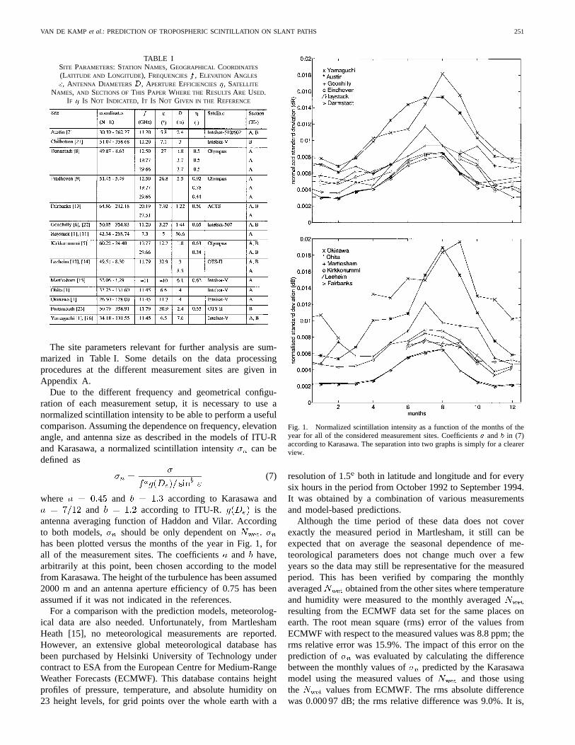
antenna averaging function of Haddon and Vilar. Accordingto both models, should be only dependent on .has been plotted versus the months of the year in Fig. 1, forall of the measurement sites. The coefficientsand have,arbitrarily at this point, been chosen according to the modelfrom Karasawa. The height of the turbulence has been assumed2000 m and an antenna aperture efficiency of 0.75 has beenassumed if it was not indicated in the references.

For a comparison with the prediction models, meteorolog-ical data are also needed. Unfortunately, from MartleshamHeath [15], no meteorological measurements are reported.However, an extensive global meteorological database hasbeen purchased by Helsinki University of Technology undercontract to ESA from the European Centre for Medium-RangeWeather Forecasts (ECMWF). This database contains heightprofiles of pressure, temperature, and absolute humidity on23 height levels, for grid points over the whole earth with a

Fig. 1. Normalized scintillation intensity as a function of the months of theyear for all of the considered measurement sites. Coefficientsa and b in (7)according to Karasawa. The separation into two graphs is simply for a clearerview.

resolution of 1.5 both in latitude and longitude and for everysix hours in the period from October 1992 to September 1994.It was obtained by a combination of various measurementsand model-based predictions.

Although the time period of these data does not coverexactly the measured period in Martlesham, it still can beexpected that on average the seasonal dependence of me-teorological parameters does not change much over a fewyears so the data may still be representative for the measuredperiod. This has been verified by comparing the monthlyaveraged obtained from the other sites where temperatureand humidity were measured to the monthly averagedresulting from the ECMWF data set for the same places onearth. The root mean square (rms) error of the values fromECMWF with respect to the measured values was 8.8 ppm; therms relative error was 15.9%. The impact of this error on theprediction of was evaluated by calculating the differencebetween the monthly values of predicted by the Karasawamodel using the measured values of and those usingthe values from ECMWF. The rms absolute differencewas 0.000 97 dB; the rms relative difference was 9.0%. It is,


Fig. 2. Monthly averagedNwet at all the sites, all from meteorologicalmeasurements, except those in Martlesham, which are from ECMWF.

therefore, expected that the ECMWF data can reasonably beused to estimate the monthly averaged of a site fromwhich no meteorological results have been reported. Fig. 2shows the monthly averaged as a function of the months,all from the measurements at the sites, except for those fromMartlesham, which have been calculated from ECMWF data.

Fig. 3 shows a scatterplot of the normalized intensity(Fig. 1) versus (Fig. 2) for all sites, months, and fre-quencies. The theoretical relation according to Karasawa isalso shown, as well as lines fitted to the data from eachsite separately. The correlation of all these results togetheris significantly worse than that of the results of each stationseparately, as can be expected. Furthermore, the gradientsof the fitted lines for the separate stations are in general ingood agreement with the model, but there is a considerablyvariable negative offset. In general, the offset is smallest inJapan (where the model came from) and largest in Europe. Itcan be concluded that Karasawa’s model predicts the seasonalvariation of the monthly average well for various placeson earth, but not the annual average.

On the first line of Table II, the correlation coefficient ofall points of Fig. 3 together is shown, as well as the rms

Fig. 3. Normalized scintillation intensity versusNwet for all of the differentsites, months, and frequencies. Theoretical relation from Karasawa (thick line)and individual linefits for the data from each site (dotted lines).

TABLE IICOMPARISON OF THEEXISTING AND PROPOSEDNEW PREDICTION MODELS:

CORRELATION COEFFICIENT OFNwet VERSUS�n FOR KARASAWA AND

ITU-R MODEL, AND OF Nwet +Q VERSUS�n FOR THE NEW MODELS

FOR ALL MEASUREMENT POINTS (MONTHLY AVERAGES), AND RMSRELATIVE ERROR OF THEMODEL-PREDICTED �n WITH RESPECT TO THE

MEASURED �n FOR ALL MEASUREMENT POINTS (MONTHLY AVERAGES)

relative error in made by the Karasawa model. The samecalculations have been made using the model parametersand in (7) according to ITU-R, the result of which is alsoshown in Table II. This result appears to be even worse thanthat from Karasawa.

The fact that the situation does not improve by changingthe frequency exponentcan be explained considering that atmost of the stations, measurements were made at a frequencybetween 11 and 12.5 GHz. The relative positions of thesemeasurement results are hardly affected by adjusting thefrequency dependent term. The same thing can be said forthe elevation angle dependent term, because different siteswith similar elevation angles gave different results. Therefore,another way of improving the situation is considered in thispaper. Further analysis is made starting from Karasawa’smodel configuration, since it gave the best result. An additionalparameter for this model is sought.

2) Improvement Using Cloud Information:It has been ob-served several times that there is a significant correlationbetween the occurrence of scintillation and the presence ofcumulus clouds along the propagation path. This gives theimpression that at least part of the turbulent activity causingscintillation is associated with cumulus clouds. As an example,Mohd Yusoffet al. [6] found a significant difference in average


scintillation intensity for their “dry” and “wet” databases fromGoonhilly and suggested that scintillation in the latter maybe caused by turbulent mixing of air masses with differentwater contents in and around clouds and precipitation. Theycalled this effect “turbulent attenuation.” The parameterat ground level is not a good indicator of this kind ofturbulence. Tervonenet al. [17] showed that the averagevariation of scintillation intensity over the hours of the dayis uncorrelated with and strongly correlated with thecumulus cloud cover. Therefore, a new parameter indicatingthe average water content of “turbulent clouds” occurringon the propagation path may help to improve the predictionmodels of scintillation.

The ECMWF database provides a possibility to derive a pa-rameter indicating the water content of turbulent clouds. Usingthe Salonen/Uppala cloud model (an improved version of themodel first published in [18] and [19]), the occurrence, height,and thickness of clouds, as well as their water content as afunction of height, can be calculated from the height profilesof pressure, temperature and humidity. This has been done forall the considered measurement sites, yielding for each sitea time series of height profiles of the cloud water content.From this information various statistical cloud properties canbe calculated.

For each site, we calculated the average water contentof heavy clouds . Here, “heavy clouds” means a cloudlayer with an integrated water content larger than 0.70 kg/m.

indicates the integrated water content (including ice)of heavy clouds averaged over only the time during whichthese occurred. On average this parameter shows a climaticcorrelation with , which, in some cases, is better than thatof ; e.g., the annual average in Darmstadt is lowerthan that in Kirkkonummi and Eindhoven as is the average

, while the average is not. A climatic correlation ofa long-term averaged parameter was exactly what was neededto improve the prediction models. has been incorporatedin a new prediction model for in the following way:

(8)

(9)

where the overscore denotes long-term (at least annual) aver-age and is expressed in kg/m. In (8), is a long-termaverage parameter and, therefore, constant for each site sothat all seasonal dependence of is still represented by

. The coefficients in (9) have been empirically adjustedto give maximum correlation between ( and . Thesignificant improvement in climatic correlation is illustrated bythe correlation coefficients of annual averages: The correlationcoefficient of annual average versus for all sites andfrequencies is 0.943; that of versus ( ) is 0.983.

A scatterplot of the monthly versus for allthe sites is shown in Fig. 4. The correlation coefficient of thepoints and the rms relative error of the new model are includedin Table II. It is evident from both Fig. 4 and Table II that theperformance of this model is considerably better than that ofthe Karasawa model for the data tested.

Fig. 4. �n versusNwet + Q for all of the different sites, months, andfrequencies. Individual line fits for the data from each site (dotted lines) andthe new proposed model (thick line).

The outliers in Fig. 4 are data points from Martlesham,which is very likely due to the fact that the meteorologicaldata for this site come from the ECMWF data set so thatthe monthly correlation between and is less goodthan that for the other sites. To illustrate this: it was checkedthat, if all values were taken from the ECMWF datainstead of from the measurements, the overall spread in Fig. 4would slightly increase and the Martlesham data would not beoutliers anymore.

The performance of the new model is better even for the datafrom Yamaguchi, Ohita, Okinawa, and Haystack, on whichKarasawaet al.had already tested their model [1]: for this datasubset, the correlation coefficient of the monthly versus( ) is 0.943 and the rms relative error of the new modelis 14.2%, while using the Karasawa model these figures are0.937 and 22.1%.

Equations (7)–(9) together now form a new empirical modelfor the prediction of monthly averaged scintillation intensity.However, much more data from more different sites, in dif-ferent climates and operating at different elevation angles andfrequencies will have to be collected in order to validate thismodel and develop a globally applicable prediction model.It shows nevertheless from the above that scintillation is, atleast partly, associated with turbulence in heavy clouds, andthat the water content of heavy clouds (water content>0.70 kg/m) is a significant indicator of the annual averagescintillation intensity, and is therefore a useful parameter tobe combined with , in order to improve the long-termperformance of global scintillation prediction models.

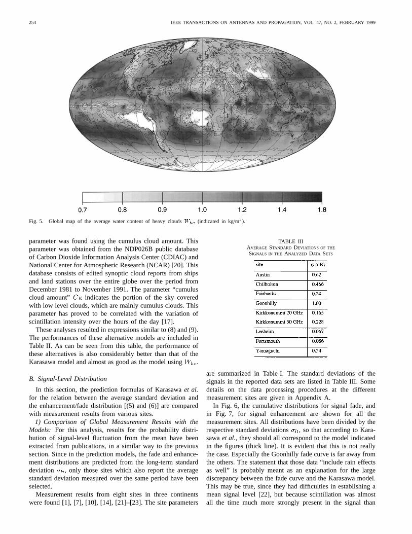
In order to make a comparison with other measurementresults possible, a global map of the long-term average watercontent of heavy clouds has been calculated from theECMWF data. The result of this is shown in Fig. 5.

The same analysis as above has been performed withthe “average probability of heavy clouds” as an extraparameter, indicating the probability of occurrence of theclouds with water content 0.70 kg/m . This parameter canalso be calculated from the ECMWF data. A third alternative


Fig. 5. Global map of the average water content of heavy cloudsWhc (indicated in kg/m2).

parameter was found using the cumulus cloud amount. Thisparameter was obtained from the NDP026B public databaseof Carbon Dioxide Information Analysis Center (CDIAC) andNational Center for Atmospheric Research (NCAR) [20]. Thisdatabase consists of edited synoptic cloud reports from shipsand land stations over the entire globe over the period fromDecember 1981 to November 1991. The parameter “cumuluscloud amount” indicates the portion of the sky coveredwith low level clouds, which are mainly cumulus clouds. Thisparameter has proved to be correlated with the variation ofscintillation intensity over the hours of the day [17].

These analyses resulted in expressions similar to (8) and (9).The performances of these alternative models are included inTable II. As can be seen from this table, the performance ofthese alternatives is also considerably better than that of theKarasawa model and almost as good as the model using.

B. Signal-Level Distribution

In this section, the prediction formulas of Karasawaet al.for the relation between the average standard deviation andthe enhancement/fade distribution [(5) and (6)] are comparedwith measurement results from various sites.

1) Comparison of Global Measurement Results with theModels: For this analysis, results for the probability distri-bution of signal-level fluctuation from the mean have beenextracted from publications, in a similar way to the previoussection. Since in the prediction models, the fade and enhance-ment distributions are predicted from the long-term standarddeviation , only those sites which also report the averagestandard deviation measured over the same period have beenselected.

Measurement results from eight sites in three continentswere found [1], [7], [10], [14], [21]–[23]. The site parameters

TABLE IIIAVERAGE STANDARD DEVIATIONS OF THE

SIGNALS IN THE ANALYZED DATA SETS

are summarized in Table I. The standard deviations of thesignals in the reported data sets are listed in Table III. Somedetails on the data processing procedures at the differentmeasurement sites are given in Appendix A.

In Fig. 6, the cumulative distributions for signal fade, andin Fig. 7, for signal enhancement are shown for all themeasurement sites. All distributions have been divided by therespective standard deviations , so that according to Kara-sawaet al., they should all correspond to the model indicatedin the figures (thick line). It is evident that this is not reallythe case. Especially the Goonhilly fade curve is far away fromthe others. The statement that those data “include rain effectsas well” is probably meant as an explanation for the largediscrepancy between the fade curve and the Karasawa model.This may be true, since they had difficulties in establishing amean signal level [22], but because scintillation was almostall the time much more strongly present in the signal than


Fig. 6. Cumulative distributions of signal fade normalized by the standarddeviations for all of the measurement sites and the model by Karasawa (thickline). The letters are initials of the names of the sites (see Table I or III forthe full names).

Fig. 7. Cumulative distributions of signal enhancement, normalized by thestandard deviations for all of the measurement sites and the model byKarasawa (thick line).

rain attenuation, it should be expected that rain was not theonly cause of this discrepancy. Another effect that is likely toplay a role in the results for Goonhilly is multipath fading dueto the layered structure of the troposphere. This effect, whichis mostly observed on line-of-sight links, can also becomesignificant on earth-space links with elevation angles belowabout 4 [3].

Since, however, also the other measurement results inFigs. 6 and 7 show significant deviations from the Karasawamodel, it is expected that the Goonhilly results are a com-bination of scintillation and multipath fading. In general, theobservations suggest that the fade and enhancement distribu-tions normalized by the standard deviations are not as constantas suggested by Karasawaet al. In the next subsection, wewill look for a physical model which explains the observedvariations of the normalized signal distributions.

Fig. 8. Theoretical distribution of normalized signal enhancement and fadefor the indicated values of the long-term standard deviation, assuming aRice–Nakagami distribution for the short-term received electric field amplitude[24].

2) Improvement:The Karasawa model for signal enhance-ment had been derived assuming a Gaussian short-term dis-tribution of signal level in decibels. Van de Kamp [24]demonstrated that this assumption is not necessarily correct.As discussed in Section III-A, the main cause of scintillationon a satellite link is turbulence in clouds. This implies that theturbulent layer is likely to be a thin layer far from the receiver.From this modeling approach, it follows that the receivedelectric field amplitude is on a short term Rice–Nakagamidistributed and the distribution of signal level in decibelsis asymmetrical [24]. This can explain the difference betweenmeasured fade and enhancement. The effect of this on the long-term distribution of is shown in Fig. 8; the normalized fadeincreases with the long-term standard deviation, while the nor-malized enhancement decreases. This agrees with the behaviorobserved in Figs. 6 and 7, which confirms the assumption ofthe thin turbulent layer and the Rice–Nakagami distribution.

The results of Figs. 6 and 7 do not quantitatively exactlymatch with the theoretical results of Fig. 8. This can be due tothe assumption of the long-term gamma distribution of theshort-term standard deviation, with , where

is the long-term mean of , generally equal to long-term standard deviation , and is the long-term standarddeviation of . This relation was stated by Karasawaet al. [1]and also used in the derivation of Fig. 8. If, however, e.g.,is in reality larger with respect to than assumed, the spreadof the gamma distribution will be larger and strong short-termfluctuations will occur more frequently for the same long-termmean standard deviation, resulting in larger normalized fadesand enhancements exceeded for small probabilities.

It could now be suggested to look for a globally applicablerelation between and . However, for this, the best waywould be to compare measured values of and fromdifferent sites, but these are not available. Instead, we willlook for a model that expresses the distributions of normalizedfade and enhancement qualitatively similar to Fig. 8. Let us


Fig. 9. The function (P )=�lt for all of the different measurement sites anda new proposed model curve (thick line).

first define

(10)

where

the distribution of signal fade (decibels);the distribution of signal enhancement (decibels).

In Fig. 9, is shown normalized by dividing it by forall the measurement sites. This corresponds to the averageof normalized fade and enhancement in Fig. 8, which isapproximately independent of there. In Fig. 9, the resultsare indeed similar for all sites except Goonhilly. A curve hasbeen fitted to these results and is indicated in the graph (thickline).

The difference between normalized fade and enhancementis approximately proportional to in Fig. 8, so isapproximately proportional to . In Fig. 10, has beenplotted for all sites, divided by . Here it is seen that theresults from the different sites almost converge. In Fairbanks,Kirkkonummi, Leeheim, and Portsmouth both andare too small for an accurate calculation. A curve has beenfitted to the results of Austin, Chilbolton, and Yamaguchi, andindicated in the graph (thick line). The fitted curves give thefollowing expressions:

(11)

(12)

where long-term standard deviation (decibels).Equations (10)–(12) now form a new model for the long-

term distribution of signal level. The advantages of this modelwith respect to Karasawa’s model are that the asymmetryof the long-term distribution is now theoretically predictedand this asymmetry increases with the scintillation intensity,consistently with measurement results.

The performance of this new model is compared with thatof Karasawa’s model in Table IV where the rms absolute and

Fig. 10. The function�(P )=�2lt

for all of the different measurement sitesand a new proposed model curve (thick line).

TABLE IVEVALUATION OF NEW MODEL OF SIGNAL FADE AND ENHANCEMENT

DISTRIBUTION: ABSOLUTE AND RELATIVE RMS ERRORS OFNEW MODEL

OVER THE RANGE 0:001% � P � 20% AND THE KARASAWA MODEL,OVER THE RANGE 0:01% � P � 20%. “TOTAL” I NDICATES THE RMSERROR OFALL RESULTS TOGETHER EXCEPT THOSE FROMGOONHILLY

relative deviations from all of the measured distributions arecompared. The probability range between 20 and 50% is notconsidered because the absolute error is small anyway andthe relative error may become unreasonably large. In thistable, the improvement with respect to the Karasawa model isevident, especially considering that for the Karasawa model theprobability range between 0.01 and 0.001% was not consideredsince the model is not defined there. The new model performsless good than the Karasawa model only in Yamaguchi, whichis for the measurements on which the Karasawa model wasbased. In Chilbolton, the absolute error of the new model isslightly larger due to values at very low probability levels. Forall other sites the new model shows a significant improvementwith respect to the Karasawa model. The improvement alsoshows clearly in Fig. 11, where the models are plotted togetherwith the measured distributions for some of the sites.

In Goonhilly, there is still a significant difference betweenthe measured fading and the new model, which can be as-cribed to multipath fading due to the layered structure of theatmosphere, as discussed before. It can, therefore, be expectedthat the new model describes turbulence induced scintillation,


(a) (b)

(c) (d)

Fig. 11. Measured and modeled distributions of fade and enhancement in (a) Austin, (b) Goonhilly, (c) Kirkkonummi (19.77 GHz), and (d) Portsmouth: —— — measured distribution, - - - - - new proposed model, and� � � � � Karasawa model. “f”= fade; “e” = enhancement.

which dominates the clear weather signal fluctuations forelevation angles above about 4. For lower elevation angles,another asymmetric component describing multipath fadingshould be added.

IV. CONCLUSIONS

It is found from a comparison of the current scintillationprediction models with available global data that is notsufficient as a single meteorological input for long-term scin-tillation intensity prediction. There are significant indicationsthat at least part of the measured scintillation is caused byturbulence in clouds. The water content of heavy clouds(water content 70 kg/m ) provides a good parameter torepresent the scintillation due to cloudy turbulence. A newscintillation prediction model using both and showsa significantly better performance than the current models. Asalternatives to , the average probability of heavy cloudsor the cumulus cloud amount may also be used.

The normalized (i.e., divided by long-term standard devia-tion) distributions of signal fade and enhancement have sig-nificantly varying shapes at various sites. This is not predictedby the Karasawa model. The theory assuming a thin turbulentlayer and a Rice–Nakagami distribution for the short-term vari-ations of electric field amplitude not only predicts the asymme-try of the long-term signal-level distribution (in contrast to thetheory of Karasawa’s model), but also predicts a dependenceof this asymmetry on the long-term standard deviation, similarto the dependence observed. A new model that takes thisdependence into account can predict the long-term distributionof signal level significantly better. At elevation angles belowabout 4 , multipath fading also contributes to the measuredsignal fluctuations, increasing the asymmetry further.

Furthermore, it is reiterated that the development of globalprediction models of both the long-term scintillation intensityand the signal-level distribution still requires much more datafrom measurement sites in different climates, and operating at


different frequencies and elevation angles, so the new modelscan be validated and improved further. The use of largeglobal databases, as done in this paper, is essential for thedevelopment of semi-empirical models as the ones discussedhere for which the physical relations are qualitatively knownto some extent but need be quantified experimentally.

At this juncture, it is proposed that the prediction modelspresented in this paper, of the long-term scintillation intensityand the long-term signal-level distribution due to scintillation,be used in the design of satellite links. For the model of thelong-term intensity, global maps of the necessary meteorolog-ical information are available, generated from the ECMWFdatabase. The information can be obtained by contacting theauthors of this paper.

APPENDIX ADETAILS ON THE DATA PROCESSINGPROCEDURES

AT THE DIFFERENT MEASUREMENT SITES

After each description is indicated in which section of thispaper the results are used.

Austin, TX [7]: The University of Texas reported mea-surements under contract with INTELSAT covering theperiod June 1988 to May 1992, during which the right-handcircularly polarized 11.20 GHz signal from a succession ofthree geostationary satellites in the same orbital locationwas monitored. The receiver output was sampled at 2 Hzand the meteorological sensors of temperature and humidityat 0.1 Hz. Slowly varying signal components were removedby subtracting the signal averaged over consecutive 6-minintervals. The standard deviation calculated over every houris reported averaged over every day and averaged overapproximately a two week period. We have averaged theseresults over each month (Section III-A). In addition, thesignal fluctuation statistics were derived from June 1988 toMay 1991. The resulting distributions have been submittedto the databank “DBSG5” of ITU-R [13] (Section III-B).Chilbolton, U.K. [21]: A satellite beacon receiving stationhas been in operation at the U.K. SERC Chilbolton Observa-tory between July 1983 and September 1984. The receivedsignal was the 11.20 GHz beacon from an INTELSAT-V satellite over the Indian Ocean. Data correspondingto periods of rain fading were excluded from analysis.Statistics of signal-level variations were made for the periodfrom July to September 1984 (Section III-B).Darmstadt, Germany [8]: The Olympus satellite beaconsignals at 12.50, 19.77, and 29.66 GHz were measured at theResearch Institute of Deutsche Bundespost Telekom (cur-rently known as the Research Centre of Deutsche TelekomAG) with two antennas of different sizes. The receiveroutputs were sampled at a rate of 80 Hz, and averaged on-line over every second. Slowly varying signal contributionscaused by attenuation due to gases, clouds, and rain wereremoved from the signal by a suitable hardware high-pass filter. Next, the signal variance was calculated overevery minute from January 1990 to December 1992, withthe exception of a few outage periods. Temperature andhumidity were recorded as well, but only data from

1992 were evaluated, since earlier measured values showeda saturation effect for relative humidities80%. Therefore,in this analysis, only the scintillation data from 1992 areused. The variances and the data were averaged overeach month (Section III-A).Eindhoven, The Netherlands[9]: The three Olympus bea-cons were received at Eindhoven University of Technologywith one Cassegrain antenna with a frequency-dependentaperture efficiency. The signal was sampled at a rate of 3Hz. The scintillation standard deviation was calculated overevery minute in the period from January 1991 to May 1992,except from June to August 1991, when Olympus was out oforder. Temperature and average humidity were also recordedover the same periods. The signal standard deviations andthe calculated values were averaged over each month(Section III-A).Fairbanks, AK [10]: Scintillation was measured in a prop-agation experiment using the 20.19 and 27.51 GHz beaconsreceived from the ACTS satellite for the period December1993 to November 1995. Beacon measurements were sam-pled at 1 Hz, a moving average over 120 s was subtractedfrom the signal, and the signal standard deviation overevery hour was calculated. Dry conditions were identifiedusing a sky temperature threshold. The standard devia-tions were averaged over the dry periods of each month.Meteorological parameters were also averaged over eachmonth (Section IIIA). In addition, the cumulative statisticsof signal level at 20.16 GHz are reported for the monthsFebruary and August 1994. We added a small offset value tothe statistics, to make the median value 0 dB (Section III-B).Goonhilly, U.K. [6]: British Telecom carried out an ex-periment under contract to the INTELSAT organizationto gather low-elevation data of tropospheric scintillation.The database, which was later analyzed in detail at Brad-ford University, Bradford, U.K., consisted of continuous10 min standard deviations of signal strength at 11.20GHz, radiometer temperature and meteorological parameterswhich were measured between February 1988 and August1990. A “dry” data subset was extracted from the data,being characterized by a radiometer temperature80K. The signal standard deviations and the meteorologicaldata were averaged over each month (Section III-A). Inaddition [22], the signals received from November 1987to October 1990 were analyzed. Difficulty was experiencedin deriving fading and enhancement statistics with a signalthat was fluctuating so significantly. The radiometer andten minute averages of the beacon level were used exten-sively to establish a nominal clear sky level. The statisticswere derived from simple addition of the total time eachthreshold was crossed, without any smoothing. The resultingdistributions have been submitted to the databank “DBSG5”[13]. With this submission, it was mentioned that the fadingdata include rain effects as well. We added a small offsetvalue to both statistics, to make the median value 0 dB(Section III-B).Haystack, MA [1], [11]: Scintillation and meteorologi-cal parameters were measured during a one-year period.The seasonal averages of scintillation standard deviation at


7.3 GHz, temperature and relative humidity are reported(Section III-A).Kirkkonummi, Finland [5]: Measurements were made ofthe beacons received from Olympus, from June 1992 toMay 1993 at 19.77 GHz and from June to October 1992at 29.66 GHz. The data were analyzed, under contract toESA, at Helsinki University of Technology by the authorsof this paper. The signal was sampled at 20 Hz and thevariance was calculated over every minute. Data for whichthe rain intensity exceeded 0.03 mm/h were excluded fromthe analysis. was calculated from the temperatureand humidity, which were measured at the site with atime resolution of one minute. Both the variances and the

data were averaged over every month (Section III-A).In addition, the fade and enhancement distributions werederived over the same periods (Section III-B).Leeheim, Germany [12]: The 11.79 GHz beacon of theorbital test satellite (OTS) was received by two differentantennas at an experimental ground station of DeutscheBundespost from June to December 1983. The postdetec-tion bandwidth was 20 Hz; the signals were sampled atintervals of 72 ms and the one minute variances werecalculated. Time periods with rain events leading to atten-uations exceeding 0.4 dB were excluded. Meteorologicalmeasurements were also performed. The monthly averagedstandard deviations and were submitted to the data-bank “DBSG5” [13]. Ortgies [14] found that thermal noisewith a standard deviation of 0.0346 dB was present in thesignal of the 3-m antenna. Therefore, we subtracted thiscontribution from the reported data for the 3-m antenna anda scaled contribution according to the Haddon/Vilar antennaaveraging function for the 8.5-m antenna (Section III-A).In addition [14], a statistical analysis was made usingthe data received by the 3-m antenna from June 1 toSeptember 13, 1983. The amplitude was sampled everytwo hours for six minutes. In total, 105 hours of datawere evaluated. Time periods with rain events leadingto attenuations exceeding 0.4 dB were excluded. Only aprobability density distribution of signal level is reported,which we converted into a cumulative distribution of signalfade and enhancement. The long-term standard deviation isassumed to be the sum of the scintillation and thermal noisestandard deviations, as reported by Ortgies (Section III-B).Martlesham Heath, U.K. [15]: A four-year study of attenu-ation, depolarization, and scintillation on an INTELSAT-Vsatellite link was conducted by British Telecom ResearchLaboratories from June 1983 to May 1987 for INTELSAT.During the measured period, four different satellites servedin succession, which were seen at elevation angles of 10.1,8.3 , 11.8 , and 10.1, respectively, and operated at 11.45and 11.20 GHz. Data were recorded each half second. Ahigh-pass filter algorithm was used to separate the rapidlyfrom the more slowly varying components of the measuredattenuation signal. The data were divided into “event” data,characterized by mean fades3 dB together with shortpre- and post-event periods, and the remaining data. Thestandard deviation was calculated over every ten minutesblock of data and averaged over each month for the “event”

data set. No meteorological measurements are reported(Section III-A).Ohita andOkinawa, Japan [1]: Measurements were madeof an INTELSAT-V beacon during the year 1983, in thesame project as the measurements at Yamaguchi (see here-after). The signal standard deviations at 11.45 GHz as wellas the temperature and relative humidity are reported, allaveraged over each month (Section III-A).Portsmouth, U.K. [23]: The 11.79 GHz beacon from theOTS was received at Portsmouth Polytechnic. For thescintillation analysis, the signal was high-pass filtered at0.01 Hz, low-pass filtered at 28 Hz, and sampled at 3 Hz. Astatistical analysis of signal level was made over a period of725 h of data between June 20 and August 1, 1980. Sincethe signal fade and enhancement statistics were very similar,cumulative statistics are reported only for signal deviation,i.e., for fade and enhancement together. Therefore, here itwill be assumed that fade and enhancement statistics wereequal for this site (Section III-B).Yamaguchi, Japan [16]: Long-term propagation experi-ments have been carried out using the INTELSAT-V satel-lite link at 11.45 GHz during the year 1983. Data weresampled at 1 Hz, and the standard deviations were calculatedover every hour, and averaged over each month. Tempera-ture, pressure, and humidity were observed four times a dayat a nearby meteorological station. From these, the wet termof the refractivity at ground level was calculated andaveraged over each month (Section III-A). In addition [1],the cumulative distributions of signal-level variations wereobtained from measurements over the months of February,May, and August, 1983. These are the data upon which theKarasawa prediction model was based (Section III-B).

REFERENCES

[1] Y. Karasawa, M. Yamada, and J. E. Allnutt, “A new prediction methodfor tropospheric scintillation on earth-space paths,”IEEE Trans. Anten-nas Propagat.,vol. 36, pp. 1608–1614, Nov. 1988.

[2] R. K. Crane and D. W. Blood, “Handbook for the estimation ofmicrowave propagation effects,” NASA Contract NAS5-25341, NASAGSFC Greenbelt, MA, Tech. Rep. 1, 7376-TR1, June 1979.

[3] ITU-R, “Propagation data and prediction methods required for the designof earth-space telecommunications systems,” Recommendations ITU-R5(F), Rec. PN 618-3, pp. 329–343, 1994.

[4] J. Haddon and E. Vilar, “Scattering Induced microwave scintillationsfrom clear air and rain on earth space paths and the influence of antennaaperture,”IEEE Trans. Antennas Propagat.,vol. AP-34, pp. 646–657,May 1986.

[5] M. M. J. L. van de Kamp, J. K. Tervonen, E. T. Salonen, and J.P. V. Poiares Baptista, “Scintillation prediction models compared tomeasurements on a time base of several days,”Electron. Lett.,vol. 32,pp. 1074–1075, 1996.

[6] M. M. B. Mohd Yusoff, N. Sengupta, C. Alder, I. A. Glover, P. A.Watson, R. G. Howell, and D. L. Bryant, “Evidence for the presenceof turbulent attenuation on low-elevation angle earth-space paths—PartI: Comparison of CCIR recommendation and scintillation observationson a 3.3� path,” IEEE Trans. Antennas Propagat.,vol. 45, pp. 73–84,Jan. 1997.

[7] W. J. Vogel, G. W. Torrence, and J. E. Allnutt, “Scintillation fading ona low elevation angle satellite path: Assessing the Austin experiment at11.2 GHz,” in8th Int. Conf. Antennas Propagat., Edinburgh, U.K., Apr.1993, Inst. Elect. Eng. Conf. Pub. 370, vol. 1, pp. 48–51.

[8] G. Ortgies, “Prediction of slant-path amplitude scintillations from me-teorological parameters,” inProc. Int. Symp. Radio Propagat., Beijing,China, Aug. 1993, pp. 218–221.


[9] S. I. E. Touw, “Analyses of amplitude scintillations for the evaluation ofthe performance of open-loop ULPC systems,” M.Sc. thesis, EindhovenUniv. Technol., The Netherlands, 1994, pp. 129–134.

[10] C. E. Mayer, B. E. Jaeger, R. K. Crane, and X. Wang, “Ka-bandscintillations: Measurements and model predictions,”Proc. IEEE,vol.85, pp. 936–945, June 1997.

[11] R. K. Crane, “Low elevation angle measurement limitations imposedby the troposphere: An analysis of scintillation observations made atHaystack and Millstone,” MIT Lincoln Lab. Tech. Rep. 518, Lexington,MA, 1976.

[12] G. Ortgies and F. Rucker, “Diurnal and seasonal variations of OTSamplitude scintillations,”Electron. Lett.,vol. 21, no. 4, pp. 143–145,1985.

[13] ITU-R, “Acquisition, presentation and analysis of data in studies oftropospheric propagation,” Recommendations ITU-R, vol. 5(A), Rec.PN 311-7, pp. 10–52, 1994.

[14] G. Ortgies, “Probability density function of amplitude scintillations,”Electron. Lett.,vol. 21, no. 4, pp. 141–142, 1985.

[15] S. M. R. Jones, I. A. Glover, P. A. Watson, and R. G. Howell, “Evidencefor the presence of turbulent attenuation on low-elevation angle earth-space paths—Part 2: Frequency scaling of scintillation intensity on a 10�

path,” IEEE Trans. Antennas Propagat.,vol. 45, pp. 85–92, Jan. 1997.[16] Y. Karasawa, K. Yasukawa, and M. Yamada, “Tropospheric scintillation

in the 11/14-GHz bands on earth-space paths with low elevation angles,”IEEE Trans. Antennas Propagat.,vol. 36, pp. 563–569, Apr. 1988.

[17] J. K. Tervonen, M. M. J. L. van de Kamp, and E. T. Salonen, “Predictionmodel for the diurnal behavior of the tropospheric scintillation variance,”IEEE Trans. Antennas Propagat., vol. 46, pp. 1372–1378, Sept. 1998.

[18] E. Salonen and S. Uppala, “New prediction method of cloud attenua-tion,” Electron. Lett.,vol. 27, no. 12, pp. 1106–1108, 1991.

[19] E. Salonen, S. Karhu, S. Uppala, and R. Hyvonen, “Study of improvedpropagation predictions,” Helsinki Univ. Technol. Finnish Meteorolog.Inst., Final Rep. ESA/Estec Contract 9455/91/NL/LC(SC), pp. 83–87,1994.

[20] C. J. Hahn, S. G. Warren, and J. London, “Edited synoptic cloud reportsfrom ships and land stations over the globe, 1982–1991,” NDP026B,Carbon Dioxide Inform. Anal. Ctr., Oak Ridge Nat. Lab., Oak Ridge,TN, 1996.

[21] O. P. Banjo and E. Vilar, “Measurement and modeling of amplitudescintillations on low-elevation earth-space paths and impact on com-munication systems,”IEEE Trans. Commun.,vol. C-34, pp. 774–780,Aug. 1986.

[22] E. C. Johnston, D. L. Bryant, D. Maiti, and J. E. Allnutt, “Results of lowelevation angle 11GHz satellite beacon measurements at Goonhilly,” in7th Int. Conf. Antennas Propagat., York, U.K., Apr. 1991, Inst. Elect.Eng. Conf. Pub. 333, vol. 1, pp. 366–369.

[23] T. J. Moulsley and E. Vilar, “Experimental and Theoretical statisticsof microwave amplitude scintillations on satellite down-links,”IEEETrans. Antennas Propagat.,vol. 30, pp. 1099–1106, June 1982.

[24] M. M. J. L. van de Kamp, “Asymmetrical signal level distributiondue to tropospheric scintillation,”Electron. Lett.,vol. 34, no. 11, pp.1145–1146, 1998.

Max M. J. L. van de Kamp (S’99) was born inDriebergen, The Netherlands, in 1963. He receivedthe M.Sc. degree in electrical engineering fromEindhoven University of Technology (EUT), TheNetherlands, in 1989.

He has been working as a Research Assistant indifferent research projects for the European SpaceAgency (ESA); he was at EUT from 1990 to 1994,at Helsinki University of Technology, Finland from1995 to 1997, and in 1997 he returned to EUT.His main activities in these projects have been in

satellite wave propagation research in the Olympus Propagation Experiment(OPEX).

Jouni K. Tervonen, for a photograph and biography, see p. 85 of the January1999 issue of this TRANSACTIONS.

Erkki T. Salonen, for a photograph and biography, see p. 85 of the January1999 issue of this TRANSACTIONS.

J. Pedro V. Poiares Baptista(M’93) was born inBeira, Mozambique. He received the Telecommuni-cations Engineering degree from the University ofOPorto, Portugal, in 1978, and the Laurea degree inelectronic engineering from Politecnico of Milan,Italy, in 1983.

He is Senior Propagation Engineer at the Euro-pean Space Research and Technology Centre of theEuropean Space Agency, Noordwijk, The Nether-lands, which he joined in 1986. Previously, he hadworked at the University of Bradford, U.K., from

1984 to 1986, Politecnico of Milan, Italy, in 1979 and again from 1981 to1983, and at Fondazione Ugo Bordoni, Rome, Italy, in 1980. Since 1978 hehas worked in the modeling of propagation effects and on the developmentof atmospheric remote sensing retrieval algorithms.

Dr. Baptista is a member of the AGU.

Improved models for long-term prediction of tropospheric...

Documents

Transcript of Improved models for long-term prediction of tropospheric...