IMPROVE STANDARD OPERATING PROCEDURES SOP 351...
68
SOP 351: Data Processing and Validation 1 IMPROVE STANDARD OPERATING PROCEDURES SOP 351 Data Processing and Validation Date Last Modified Modified by: 12/9/96 EAR 10/9/97 PHW
Transcript of IMPROVE STANDARD OPERATING PROCEDURES SOP 351...

SOP 351: Data Processing and Validation 1
IMPROVESTANDARD OPERATING PROCEDURES
SOP 351Data Processing and Validation
Date Last Modified Modified by:12/9/96 EAR10/9/97 PHW

SOP 351: Data Processing and Validation 2
SOP 351 Data Processing and Validation
TABLE OF CONTENTS1.0 PURPOSE AND APPLICABILITY ...................................................................... 42.0 RESPONSIBILITIES .............................................................................................5
2.1 Project Manager.................................................................................................. 52.2 Quality Assurance Manager................................................................................. 52.3 Quality Assurance Specialist................................................................................ 52.4 Field Specialist.................................................................................................... 52.5 Laboratory Manager ...........................................................................................62.5 Spectroscopist .................................................................................................... 6
3.0 REQUIRED EQUIPMENT AND MATERIALS .................................................... 74.0 METHODS ............................................................................................................ 8
4.1 Level 1 validation: Sampling validation.............................................................84.1.1 Sampler equipment validation....................................................................... 84.1.2 Filter validation............................................................................................84.1.3 Collection parameters.................................................................................. 94.1.4 Gravimetric and laser analysis validation..................................................... 10
4.2 Level II Validation............................................................................................ 114.2.1 Flow rate consistency checks..................................................................... 114.2.2 Quality assurance of gravimetric analyses.................................................. 124.2.3 Quality assurance of elemental analyses..................................................... 13
4.2.3.1 X-Ray Fluorescence analyses..............................................................144.2.3.2 Proton Induced X-Ray Emission and Proton Elastic Scattering Analysis154.2.3.3 Elemental data quality assurance.........................................................164.2.3.4 Quality assurance of flow rate data.......................................................................................................................Error! Bookmark not defined.
4.2.4 Quality assurance of contractor analysis.........Error! Bookmark not defined.4.3 Level III Validation..............................................Error! Bookmark not defined.
4.3.1 A channel versus B channel data...................Error! Bookmark not defined.4.3.2 A channel versus C channel data...................Error! Bookmark not defined.4.3.3 A channel versus D channel data...................Error! Bookmark not defined.4.3.4 Regional data review.....................................Error! Bookmark not defined.4.3.5 Site summary review....................................Error! Bookmark not defined.4.3.6 Final data review and validation....................Error! Bookmark not defined.
4.4 Modification and Documentation of Parameters..Error! Bookmark not defined.4.4.1 Main screen displays.....................................Error! Bookmark not defined.
4.4.1.1 Data Summary.......................................................................................................................Error! Bookmark not defined.4.4.1.2 Control Options.......................................................................................................................Error! Bookmark not defined.

SOP 351: Data Processing and Validation 3
4.4.1.3 Artifact Summary.......................................................................................................................Error! Bookmark not defined.
4.4.2 Subscreens ...................................................Error! Bookmark not defined.4.5 Calculations........................................................Error! Bookmark not defined.
4.5.1 Flow Equations ............................................Error! Bookmark not defined.4.5.1.1 The Effect of Flow Rate on Cyclone Cut Point..........................................................................Error! Bookmark not defined.4.5.1.2 Flow Control by a Critical Orifice..........Error! Bookmark not defined.4.5.1.3 Flow Rate through an Orifice Meter .......Error! Bookmark not defined.4.5.1.4 Pressure-Elevation Relationship..............Error! Bookmark not defined.4.5.1.5 Calibration of Audit Devices...................Error! Bookmark not defined.4.5.1.6 Nominal Flow Rate Equation..................Error! Bookmark not defined.4.5.1.7 Flow Rate Equation for the System Vacuum Gauge..........................................................................Error! Bookmark not defined.4.5.1.8 Calibration of the System Orifice Meter and Vacuum Gauge..........................................................................Error! Bookmark not defined.
4.5.2 Determination of Concentration, Artifacts and Precision..............................................................................Error! Bookmark not defined.
4.5.2.1 Artifact...................................................Error! Bookmark not defined.4.5.2.2 Verification by Distributions...................Error! Bookmark not defined.4.5.2.3 Definitions of Variables..........................Error! Bookmark not defined.4.5.2.4 Concentration.........................................Error! Bookmark not defined.4.5.2.5 Volume ..................................................Error! Bookmark not defined.4.5.2.6 Analytical Precision................................Error! Bookmark not defined.4.5.2.7 Gravimetric Mass...................................Error! Bookmark not defined.4.5.2.8 PIXE, XRF, and PESA Analysis.............Error! Bookmark not defined.4.5.2.9 Ion, Carbon and SO2 Analysis.................Error! Bookmark not defined.4.5.2.10 Optical Absorption ...............................Error! Bookmark not defined.
4.5.3 Equations of Composite Variables................Error! Bookmark not defined.4.5.3.1 Sulfate by PIXE (S3) and Ammonium Sulfate (NHSO)..........................................................................Error! Bookmark not defined.4.5.3.2 Ammonium Nitrate (NHNO)..................Error! Bookmark not defined.4.5.3.3 SOIL ......................................................Error! Bookmark not defined.4.5.3.4 Non-soil Potassium (KNON)..................Error! Bookmark not defined.4.5.3.5 Light-Absorbing Carbon (LAC)..............Error! Bookmark not defined.4.5.3.6 Ambient Coefficient of Absorption (BABS)Error! Bookmark not defined.4.5.3.7 Organics by Carbon (OMC)....................Error! Bookmark not defined.4.5.3.8 Organics by Hydrogen (OMH) ...............Error! Bookmark not defined.4.5.3.9 Reconstructed Mass from the Teflon filter (RCMA)..........................................................................Error! Bookmark not defined.4.5.3.10 Reconstructed Mass using Carbon Measurements (RCMC)..........................................................................Error! Bookmark not defined.
4.5.4 Statistical calculation....................................Error! Bookmark not defined.4.5.4.1 Slope and Intercept for Perpendicular FitError! Bookmark not defined.

SOP 351: Data Processing and Validation 4
4.5.4.2 Pair-wise Precision................................Error! Bookmark not defined.4.5.4.3 Pair-wise Chi-Square.............................Error! Bookmark not defined.
4.6 Transfer of Data to Final Concentrations DatabaseError! Bookmark not defined.
Technical Referencesnone
SOP 351: Data Processing and Validation 5
1.0 PURPOSE AND APPLICABILITY
This standard operating procedure (SOP) provides a general overview of the procedures forprocessing and validating IMPROVE data.
Data processing and data validation are performed in parallel. Most data validation checks areperformed as part of the data processing procedures.

SOP 351: Data Processing and Validation 6
2.0 RESPONSIBILITIES
2.1 Project ManagerThe project manager shall:
• oversee all aspects of the program• review the seasonal quality assurance summary of the quality assurance specialist to
determine if the data are acceptable for incorporation in the concentrations database
2.2 Quality Assurance ManagerThe quality assurance manager shall:
• oversee all aspects of the program pertaining to quality assurance• supervise the work of the quality assurance specialist• review the seasonal quality assurance summary of the quality assurance specialist to
determine if the data are acceptable for incorporation in the concentrations database
2.3 Quality Assurance SpecialistThe quality assurance specialist shall:
• review the site configuration database for current flow rate calibrations• review the site problems database for potential problems• review the collection parameters in the database• review the quality assurance summaries of the lab manager and the spectroscopist• review the quality assurance summaries of the external contractors• calculate concentrations and store in temporary database• run appropriate level 2 data validation programs• verify that there were no inconsistencies in analytical calibration• examine individual inconsistent samples and determine the cause• update the database with revised information (modify parameters or invalidate)• recalculate concentrations• rerun data validation programs• present a quality assurance summary for each season with appropriate plots and tables to
the quality assurance manager and project manager• transfer the data to the final concentrations database
2.4 Field SpecialistThe field specialist shall:
• maintain documentation on the flow rate calibration for each module• verify that the flow rates are within acceptable tolerances

SOP 351: Data Processing and Validation 7
2.5 Laboratory ManagerThe lab manager shall:
• oversee and maintain records on site and sampler operation• review all log sheets for completeness, and to check the validity of the samples prior to
downloading of the samples by lab technicians.• resolve any inconsistencies on the log sheet or in the samples• oversee entry of collection parameters in data base• oversee entry of gravimetric analysis parameters in data base• maintain documentation on daily gravimetric controls
2.5 SpectroscopistThe spectroscopist shall:
• maintain records on the operation and performance of the various analytical systems• maintain documentation on standards and reanalysis for each analytical session• oversee all technicians performing analyses and verify the correctness of the data entry

SOP 351: Data Processing and Validation 8
3.0 REQUIRED EQUIPMENT AND MATERIALSnone.
SOP 351: Data Processing and Validation 9
4.0 METHODS
This section deals with collection parameters of samples taken by the IMPROVE particulatesampler. These include the sampler and sample validation at levels 1 and 2.
4.1 Level 1 validation: Sampling validation
Four types of validation occur before filters and samples are accepted as valid.
Sampler equipment validation. (section 4.1.1)Filter contamination validation (section 4.1.2)Collection parameter validation (section 4.1.3)Gravimetric and laser analysis validation (section 4.1.4)
4.1.1 Sampler equipment validation.
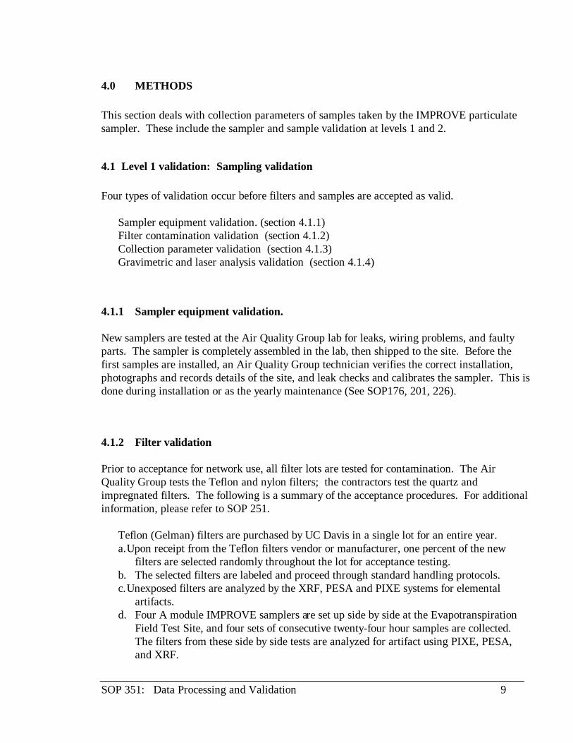
New samplers are tested at the Air Quality Group lab for leaks, wiring problems, and faultyparts. The sampler is completely assembled in the lab, then shipped to the site. Before thefirst samples are installed, an Air Quality Group technician verifies the correct installation,photographs and records details of the site, and leak checks and calibrates the sampler. This isdone during installation or as the yearly maintenance (See SOP176, 201, 226).
4.1.2 Filter validation
Prior to acceptance for network use, all filter lots are tested for contamination. The AirQuality Group tests the Teflon and nylon filters; the contractors test the quartz andimpregnated filters. The following is a summary of the acceptance procedures. For additionalinformation, please refer to SOP 251.
Teflon (Gelman) filters are purchased by UC Davis in a single lot for an entire year.a.Upon receipt from the Teflon filters vendor or manufacturer, one percent of the new
filters are selected randomly throughout the lot for acceptance testing.b. The selected filters are labeled and proceed through standard handling protocols.c.Unexposed filters are analyzed by the XRF, PESA and PIXE systems for elemental
artifacts.d. Four A module IMPROVE samplers are set up side by side at the Evapotranspiration
Field Test Site, and four sets of consecutive twenty-four hour samples are collected.The filters from these side by side tests are analyzed for artifact using PIXE, PESA,and XRF.
SOP 351: Data Processing and Validation 10
e.The Quality Assurance Manager interprets each test result and determines whether thenew lot is acceptable. If no unusually large outliers are observed, the lot is certified asfree of artifact.
f. When certified, the entire lot is accepted for use in Air Quality Group operations andpayment to the vendor is authorized.
Gelman Nylasorb nylon filter material is purchased by UC Davis in 8.5" by 11" sheetsfrom a single lot.
a. One 25 mm filter is punched from each sheet and the pressure drop for each filter isrecorded to verify that the material is uniform throughout the lot.
b. Twenty filters are sent to the ion contractor to verify that there are no abnormalartifacts.
c. The Quality Assurance Manager interprets each test result and determines whether thenew lot is acceptable. If no unusually large outliers are observed, the lot is certifiedfor use.
d. Once accepted, filters are prepared from the sheets, four sheets at a time, and storedwith spacers in standard 25 mm storage containers until required for use.
e. The remaining sheet stock is kept in a sealed container in a cool, dry, clean place untilneeded.
Quartz filters for fine carbon aerosols are purchased, pre-fired, and analyzed for artifact by anexternal contractor. Specific requirements and procedures are included in the IMPROVESOP's Appendix 13. The pre-fired quartz filters are received and retained in a clean, cool, dryenvironment until required in the loading sequence.
Impregnated filters for measuring gaseous SO2 as SO4 are both supplied and analyzed forartifact by an external contractor. Specific requirements and procedures are included in theIMPROVE SOP Appendix 14. The impregnated filters are received and retained in a clean,cool, dry environment until required in the loading sequence.
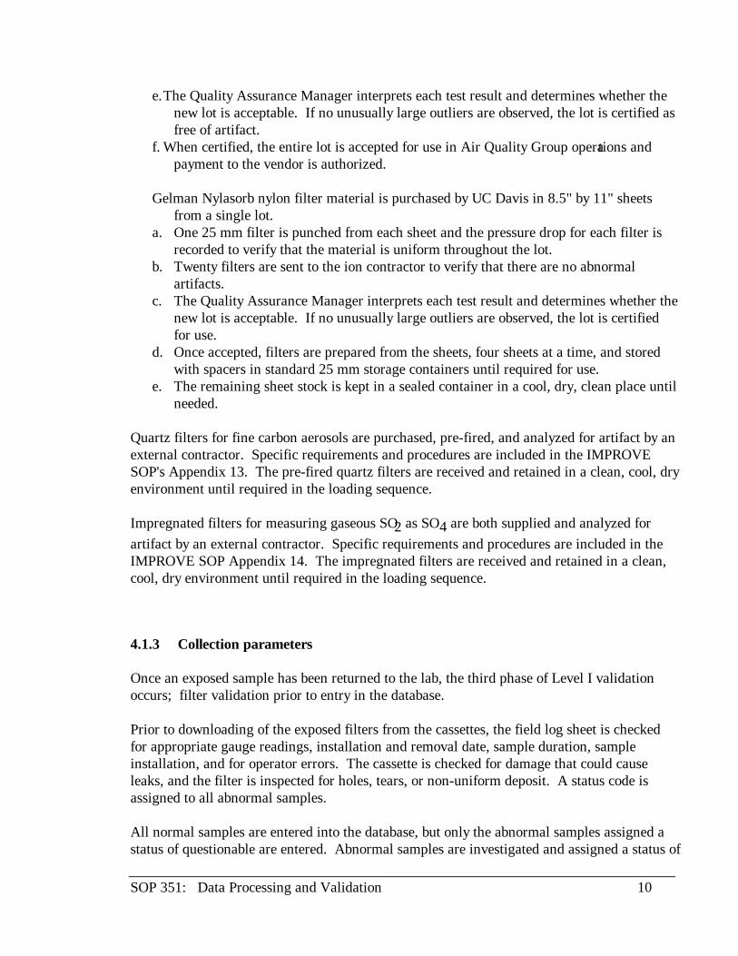
4.1.3 Collection parameters
Once an exposed sample has been returned to the lab, the third phase of Level I validationoccurs; filter validation prior to entry in the database.
Prior to downloading of the exposed filters from the cassettes, the field log sheet is checkedfor appropriate gauge readings, installation and removal date, sample duration, sampleinstallation, and for operator errors. The cassette is checked for damage that could causeleaks, and the filter is inspected for holes, tears, or non-uniform deposit. A status code isassigned to all abnormal samples.
All normal samples are entered into the database, but only the abnormal samples assigned astatus of questionable are entered. Abnormal samples are investigated and assigned a status of

SOP 351: Data Processing and Validation 11
either unusable or questionable. Unusable samples are archived without analysis and arestored separately.
Status codes indicating an unusable sample, one that is never entered into the database, are asfollows:
NS: not serviced. The samples were either exposed for more than one sampling period,or for less than 75% of their normal sampling period. The operator did not servicethe site.
EP: equipment problem. A sampler malfunction made the samples invalid.
SE: site error. The filters were incorrectly installed by the operator.
PO: power outage. The sampler ran for less than 75% of a normal sampling period dueto a power outage.
XX: invalid for other reasons. The sample ran for less than 18.00 hours, the filter has ahole, the filter has obvious problems (not centered properly, grill upside down), thefilter was dropped or contaminated by water, the cassette is broken.
Samples that are questionable are processed normally, but the data is flagged and checkedduring the data validation procedures. The status codes and the accompanying reasons forincluding a sample in these categories are:
CG: clogged filter. The final magnehelic reading is less than 1/2 of the initial reading,resulting in unreliable flow rate measurements. (This sample is kept to documentthe factors involved in clogging,)
LB: laboratory blank. A quality assurance filter used to determine artifact levels dueto laboratory procedures. It is not sent to the field, and it never samples air.
FB: field blank. A quality assurance filter used to determine artifact levels from theentire sampling process. It is handled as a normal filter, but it never samples air.
4.1.4 Gravimetric and laser analysis validation
Gravimetric analysis validation involves monitoring the precision and stability of the Cahnelectrobalances. Twice per day, at 8:30 am and 1:30 p.m., the electrobalances are cleaned andcalibrated. In the calibration procedure, the range is set, then the calibration standard weightis measured. If the standard weight is within two micrograms of it's average value and thecalibration is stable, the electrobalance is considered calibrated. If either condition is not met,the balance is checked for malfunctions and repaired if necessary. The calibrations are
SOP 351: Data Processing and Validation 12
recorded in a log with data on the humidity, temperature, and magnetic field strength duringcalibration.The zero value for the balance is checked after every five analyses. A change in the balancezero of one microgram or more during use may indicate a change in the calibration. When achange is observed, the balance is re-calibrated.
The hybrid integrating plate (HIP), laser analysis, validation involves monitoring the stabilityof the laser and detectors. Prior to the quarterly analysis, the laser and detectors are allowedto warm up for at least three hours. The laser is calibrated, and intensity in the forward andreflectance detectors is verified and recorded in the analysis log. The B93 Washington DCtray is analyzed in the laser system, and the values compared with previous analyses of thattray. If the correlation of the old and new analyses is good, the system is assumed to beoperational. If the correlation is poor, the detectors, power supply, or alignment are checkedand corrected.
During actual analysis, the laser intensity in the forward and reflectance detectors is monitoredat the start and end of each analysis tray, and after every ten samples. If the intensity changesmore than 1%, the laser is re-calibrated, and the previous ten samples are re-analyzed.
4.2 Level II Validation
Level II validation refers to quality assurance performed on measured or derived data in theTrayfile database. The five areas of verification are as follows:
flow rate consistency checks, (section 4.2.1)quality assurance of gravimetric analyses (section 4.2.2)quality assurance of laser analysis (section 4.2.3)elemental analyses (section 4.2.4)contractor analyses (section 4.2.5)
4.2.1 Flow rate consistency checks
Flow rate consistency checks are done upon entry of the field log sheet data, and at weekly,monthly and quarterly intervals for each site. If the initial flow rate is not within 5% of thenominal value, there may be a problem with the sample, or the sampler. These anomalousdata are carefully checked to determine the cause and resolution of the problem, andcorrective action is taken if necessary. If it becomes necessary, audits can be done throughthe mail (See SOP 176). The IMPROVE sampler is constructed with two independent gaugesfor flow measurements. If the primary gauge is determined to be malfunctioning, the databasemanager is notified to set the flow data pointer in the database to the secondary gauge.
SOP 351: Data Processing and Validation 13
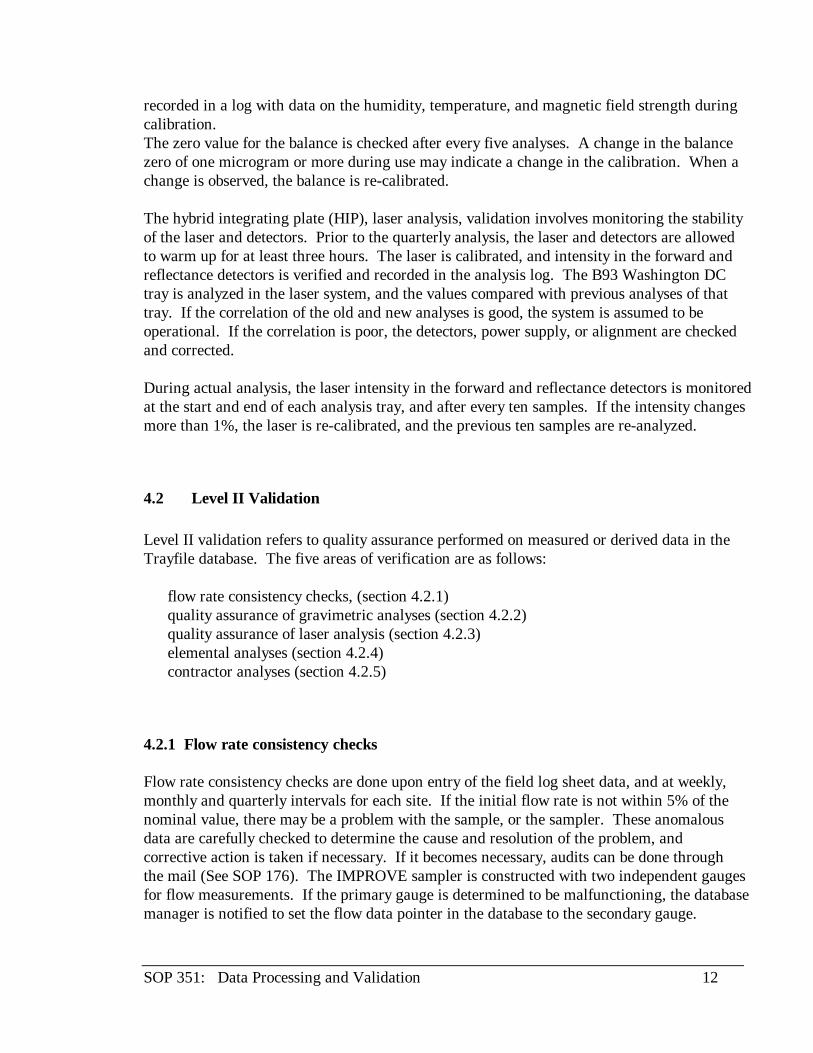
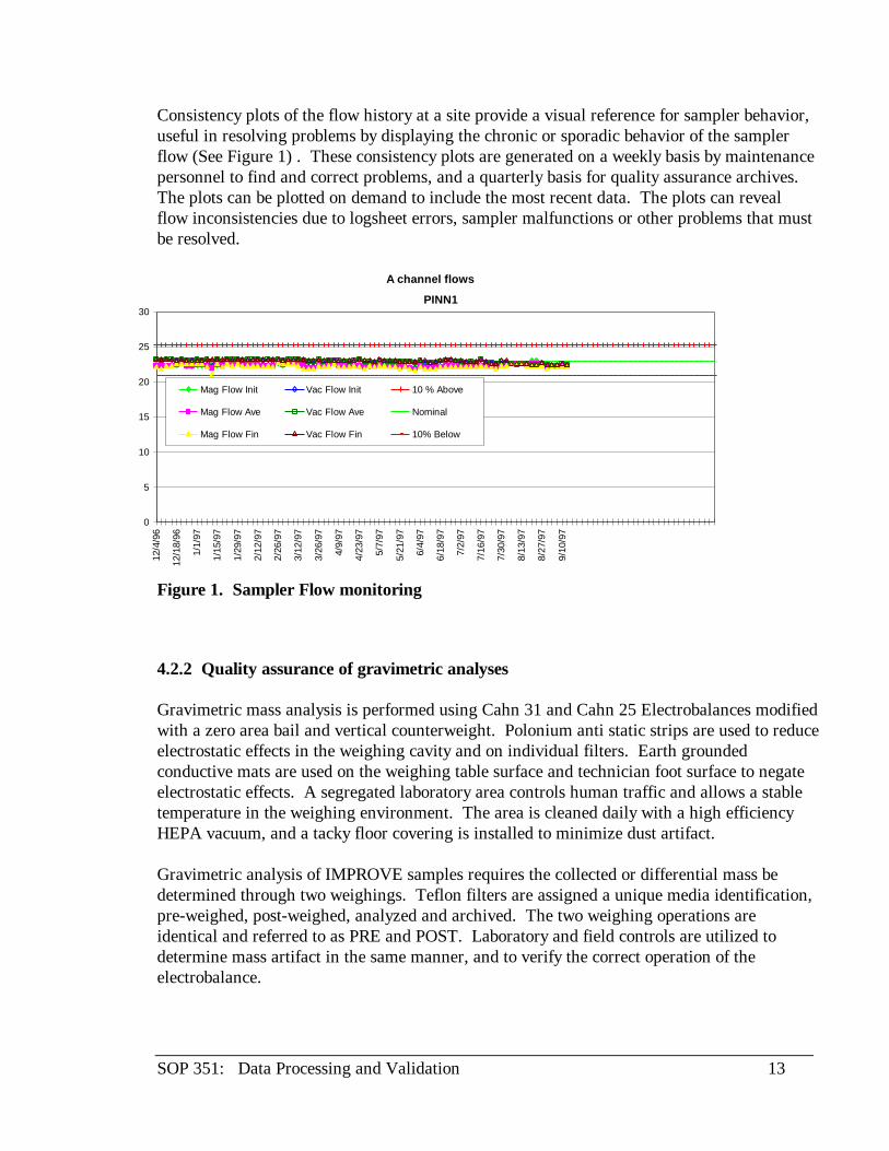
Consistency plots of the flow history at a site provide a visual reference for sampler behavior,useful in resolving problems by displaying the chronic or sporadic behavior of the samplerflow (See Figure 1) . These consistency plots are generated on a weekly basis by maintenancepersonnel to find and correct problems, and a quarterly basis for quality assurance archives.The plots can be plotted on demand to include the most recent data. The plots can revealflow inconsistencies due to logsheet errors, sampler malfunctions or other problems that mustbe resolved.
Figure 1. Sampler Flow monitoring
4.2.2 Quality assurance of gravimetric analyses
Gravimetric mass analysis is performed using Cahn 31 and Cahn 25 Electrobalances modifiedwith a zero area bail and vertical counterweight. Polonium anti static strips are used to reduceelectrostatic effects in the weighing cavity and on individual filters. Earth groundedconductive mats are used on the weighing table surface and technician foot surface to negateelectrostatic effects. A segregated laboratory area controls human traffic and allows a stabletemperature in the weighing environment. The area is cleaned daily with a high efficiencyHEPA vacuum, and a tacky floor covering is installed to minimize dust artifact.
Gravimetric analysis of IMPROVE samples requires the collected or differential mass bedetermined through two weighings. Teflon filters are assigned a unique media identification,pre-weighed, post-weighed, analyzed and archived. The two weighing operations areidentical and referred to as PRE and POST. Laboratory and field controls are utilized todetermine mass artifact in the same manner, and to verify the correct operation of theelectrobalance.
A channel flows
0
5
10
15
20
25
30
12/4
/96
12/1
8/96
1/1/
97
1/15
/97
1/29
/97
2/12
/97
2/26
/97
3/12
/97
3/26
/97
4/9/
97
4/23
/97
5/7/
97
5/21
/97
6/4/
97
6/18
/97
7/2/
97
7/16
/97
7/30
/97
8/13
/97
8/27
/97
9/10
/97
Mag Flow Init Vac Flow Init 10 % Above
Mag Flow Ave Vac Flow Ave Nominal
Mag Flow Fin Vac Flow Fin 10% Below
PINN1
SOP 351: Data Processing and Validation 14
The initial quality assurance on gravimetric data is done upon entry of pre and post weightsinto the database. The technician weighing the filters checks the site, date, and mediaidentification number and verifies the recorded mass. After post weighing, the differentialmass (post weight minus pre weight) is derived by the computer, but must be accepted by thetechnician as a reasonable, non-negative number before it is recorded in the database.
Unusual differential masses are generally resolved before entering the database. If noresolution is found, the A module mass data is flagged, but is entered into the database. Laterquality assurance procedures will deal with the problem. For D module filters, unresolvedlarge negative masses are changed in status to XX and removed to the problem file, whileunresolved large positive masses are flagged, but kept and entered into the database forfurther analysis.
The secondary quality assurance on gravimetric data occurs quarterly during construction ofthe PIXE instruction files. The differential masses are sorted by magnitude, and extremelylarge or negative masses are re-weighed for verification. Other possibilities such as samplemis-identification are considered, and the data are corrected if necessary. Also, the A channelgravimetric data, 2.5µm cut point, are compared to the D channel gravimetric data, 10µm cutpoint. If the A module gravimetric mass is the same size or larger than the corresponding Dmodule mass, both are re-weighed and flagged if no resolution occurs. No data are removedfrom the database at this time. Filters with unresolved mass problems are analyzed normally.
The final Level II verification of mass data occurs after acquiring and processing the elementaldata. Reconstructed mass values are generated from the elemental output from the elementalanalysis, and these values are compared to the measured mass values. The measured andreconstructed mass should correlate well, with the reconstructed mass being between 85%and 100% of the measured mass. The percentage is site dependent and is generally reflectedin historical data. If the percentage is substantially different from past values, or is out ofrange, there may be a problem with the weight measurement or the elemental analysis. Thesampler flow, the sample duration, and the deposit area would be carefully verified, as well asthe calibration values and re-analysis data from the PIXE run. The data manager and qualityassurance manager would investigate and a resolution reached.
If all but one or two of the measured mass values at a site correlate well with thereconstructed mass values, the measured mass for these one or two points is consideredsuspect. If the A module gravimetric mass is larger than the D module gravimetric mass forthe site and date in question, the A module gravimetric mass is assumed invalid and is flaggedfor deletion. If no clear decision can be made, the data manager is consulted and a resolutionis reached.
4.2.3 Quality assurance of elemental analyses

SOP 351: Data Processing and Validation 15
Three analytical systems are used for elemental analysis of the Teflon filters. IMPROVE Amodule (2.5µm cut point) Teflon filters are analyzed in quarterly batches. All elementalanalyses occurs during two quarterly analysis runs. The analyses and the quality assuranceprocedures associated with each can be found in the following sections:
X-Ray Fluorescence analysis, XRF, (section 3.2.3.1);Proton Induced X-Ray Emission analysis, PIXE, and Proton Elastic Scattering Analysis,PESA (section 3.2.3.2);Elemental data quality assurance (section 3.2.3.3);Quality assurance of flow rate data (section 3.2.3.4)
Upon completion of these procedures, but before deleting invalid data, the data manager isconsulted for approval. If approved, the data are deleted, and the deletions recorded in a logfile for later reference. Only one deletion file for PIXE, PESA and XRF data is created foreach quarter, and this is also saved for later reference. All of the quality assurance plots arereviewed by the data manager and archived for later reference.
4.2.3.1 X-Ray Fluorescence analyses
At the start of the analysis run, a tray of elemental standards is analyzed to provide data on thefunctioning of the XRF system, and to ensure the detector is working properly. Theseventeen elemental standards purchased from Micro Matter Co. are the same type used forPIXE standards, and are analyzed in the PIXE system every twelve analysis runs to confirmthe correlation between the XRF and PIXE systems shown by the re-analysis data. Theelemental standards include single, double, and multiple element thin film standards and rangein concentration from 20 to 60 micrograms per square centimeter. These standards areanalyzed to ensure the detector is working properly, and to calibrate the acquisition system.The same standards are used for each quarterly analysis to provide continuity. Included in thestandards tray are several unexposed filters, blanks, for determining the background spectra.The spectra of each blank is scrutinized for contaminants, and the cleanest blank is selectedfor use as the background subtract value. As a second check, this background subtract valueis used on the re-analysis samples. If the spectra are not under or over subtracted, the blank issaved.
Once the standards have been deemed acceptable, two trays of samples analyzed during theprevious run are re-analyzed. The data from this re-analysis is plotted against the data fromthe previous run. From the comparison of the standards, a re-normalization parameter, orRENO is determined. With the RENO applied to the re-analysis, the re-analyzed filters arecompared to the data set taken during the previous run. This is a calibration value thatremoves the effect of variations in the x-ray beam between analysis runs. The re-analysis trayis run at the start and end of each ten day analysis period, roughly every thousand samples, orwhenever the XRF system is shut off and turned back on. The analysis is done in ten daysegments since the XRF system must be shut down and the detector refilled with liquidnitrogen on that time scale.
SOP 351: Data Processing and Validation 16
Once the XRF system has been turned off, it requires a three hour warm up period to allowthe detector and the x-ray source to stabilize before it can be calibrated. Before continuingthe analyses, the re-analysis tray must be analyzed and a new re-normalization parametercalculated. Generally, just before the XRF system is shut down, the re-analysis tray isanalyzed to verify the current re-normalization factor.
Two system are used to collect and analyze the spectra from the detector. ACE collects thedata from the detector and associates it with an analysis number. RACE processes the datafrom the detector into a file containing the sample identification, the quantity of each speciesfound, the minimum detectable limits for each species (MDL), and the location and probableidentification of peaks in the X-ray spectrum. It also does subtraction of the backgroundvalue for the substrate. Users enter the run calibration values, and determine the optimalblank subtract. The output data is saved in files according to site and quarter or month, datafor each sample given by the operator and the analysis instruction file.
Once the data have been collected, they are stored pending PIXE analysis of the samples.Further quality assurance analysis occurs in conjunction with PIXE data quality assurance, andwill be discussed at that time.
4.2.3.2 Proton Induced X-Ray Emission and Proton Elastic Scattering Analysis
At the start and end of each analysis run, a tray of standards is analyzed. Thirty are elementalstandards purchased from Micro Matter Co., six are Mylar blanks for PESA calibration, andtwo are unused (blank) Teflon filters. The elemental standards include single, double, andmultiple element thin film standards and range in concentration from 20 to 60 micrograms persquare centimeter. These standards are analyzed to ensure the detectors are workingproperly, to normalize the two PIXE detectors, and to calibrate the acquisition system. Thesame standards are used for each quarterly analysis to provide continuity. Every twelveanalysis runs, the PIXE standards are analyzed in the XRF system and the PIXE system, andthe results are compared to confirm the correlation between the two systems shown by the re-analysis data. The areal density the elements on the standards are measured and compared tothe quoted values. The average of the ratio of the measured and quoted values is the re-normalization factor, RENO, for the analysis run, and negates differences between runs due toslight changes in the proton beam. If the RENO's are not between 0.9 and 1.1, with astandard deviation of less than 5%, the system is not considered adequate for sample analysisand the run is stopped until the problem can be rectified.
Once the standards have been deemed acceptable, a tray of samples analyzed during theprevious run is re-analyzed. The data from the re-analysis is plotted against the data from theoriginal analysis. From this comparison, an independent set of re-normalization factors,RENO's, is determined. The RENO's generated from the standards tray analysis and from there-analysis tray should agree. If the values are not within 5%, the proton beam is checked forstability, and both trays are re-analyzed.

SOP 351: Data Processing and Validation 17
The re-analysis tray is analyzed every thousand samples, roughly three times during a standardanalysis run, and whenever the proton beam is re-tuned. Generally, the same proton beam isused for an entire analysis run, so the re-analysis tray is run only three times. Re-normalization factors for the entire run are determined after the run is completed by doing bestfit analysis after averaging all the collected RENO values.
The unexposed Teflon filters, blanks, in the standards tray are used to determine the PIXEbackground spectra. The spectra of each blank is scrutinized for contaminants, and thecleanest blank is selected for use as the background subtract value. As a second check, thisbackground subtract value is tested on the re-analysis samples. The blank subtract shouldeliminate the background spectra that exist between elemental peaks, but should not eliminateany peaks.
Two system are used to collect and analyze the spectra from the detectors. ACE collects thedata from each detector and associates it with an analysis number. RACE processes the datafrom each detector into separate files containing the sample identification, the quantity of eachspecies found, the minimum detectable limits for each species (MDL), and the location andprobable identification of peaks in the X-ray spectrum. It also does subtraction of thebackground value for the substrate. Users enter the run calibration values, and determine theoptimal blank subtract. The output data is saved in files according to site and quarter ormonth, data given by the trayfile for each sample.
4.2.3.3 Elemental data quality assurance
Once the PIXE data have been collected, quality assurance procedures for the completeelemental analysis of the samples begins. This is usually done during the PIXE analysis run toreduce the chances of having a run that go beyond standard specifications. First, the XRF,then the PIXE and PESA data are re-examined to verify the calibration and blank subtractvalues used during the analysis runs. Parallel data sets are created, the XRF database havingonly XRF data, the PIXE database containing PIXE data , and PESA database containing thePESA data. A plotting program is used to compare the following species from each databasefor each sample: S, Ca, K, V, Ti, Mn, Fe, Ni, Cu, Zn, As, Pb, Se, Br, Sr, Rb, and Zr (SeeFigure 2). If the species do not correlate well, the data manager and PIXE manager areconsulted. The calibrations and re-analysis data are checked, and a resolution is reached.
If the species all show good correlation, the following correlation plots are created:gravimetric mass versus reconstructed mass,(MF vs. RCMA),

SOP 351: Data Processing and Validation 18
Figure 2. PIXE vs. XRF comparison
gravimetric mass versus hydrogen, (MF vs. H), andsilicon versus iron, (Si vs. Fe).copper versus minimum detectable limit for copper (Cu vs. Mdl)zinc versus minimum detectable limit for zinc (Zn vs. Mdl)trace element concentration versus time
As these species should correlate well, poorly correlated data points are identified andscrutinized. If the stray points appear due to regional effects (i.e. seen at most of the sites in aregion on or near that date), the data is considered valid. If the stray points do not appear tocorrelate to anything, it is possible that the data are incorrect.
A series of time plots of trace element concentration at each site are generated for thefollowing species:
Se, Br, V, Pb, Ni, and As
B96ELE, N = 1758, R = 0.998, R^2 = 0.996Y = 0.9916*X + (-2.7926), Slope error = 0.002, Intcpt. error = 2.764
Mean X = 715.08, Error = 25.24, Std Dev. = 1058.10Mean Y = 706.27, Error = 25.02, Std Dev. = 1049.21
Mean Y/Mean X = 0.988
0
2000
4000
6000
8000
10000
12000
14000
0 2000 4000 6000 8000 10000 12000 14000
IMPROVE* PFE
IMP
RO
VE
* FE
SOP 351: Data Processing and Validation 19
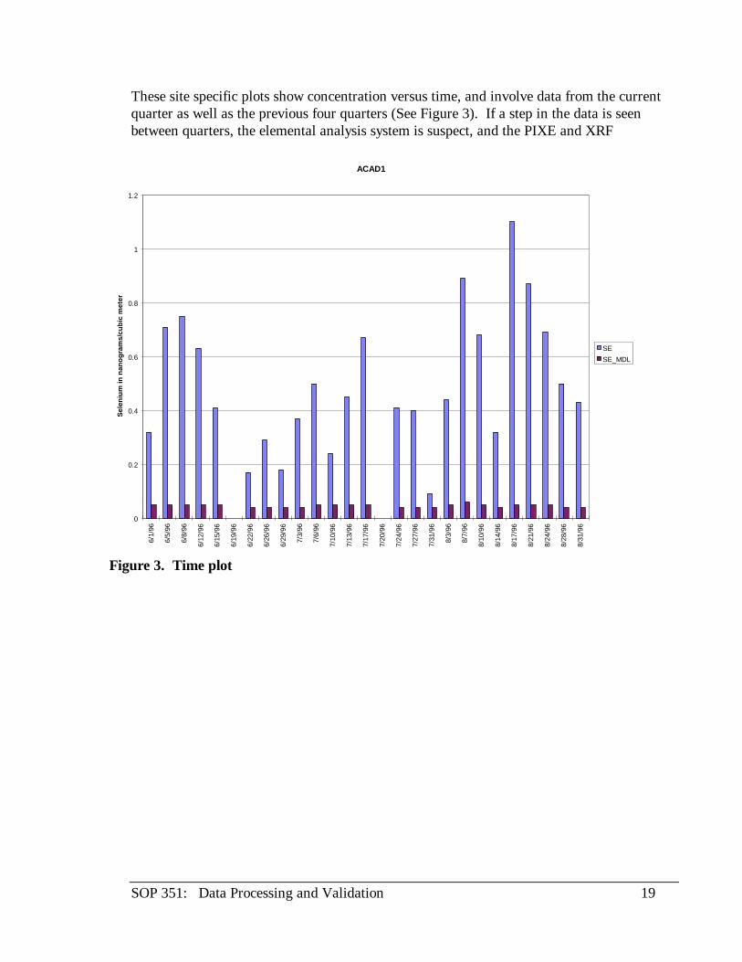
These site specific plots show concentration versus time, and involve data from the currentquarter as well as the previous four quarters (See Figure 3). If a step in the data is seenbetween quarters, the elemental analysis system is suspect, and the PIXE and XRF
ACAD1
0
0.2
0.4
0.6
0.8
1
1.2
6/1/
96
6/5/
96
6/8/
96
6/12
/96
6/15
/96
6/19
/96
6/22
/96
6/26
/96
6/29
/96
7/3/
96
7/6/
96
7/10
/96
7/13
/96
7/17
/96
7/20
/96
7/24
/96
7/27
/96
7/31
/96
8/3/
96
8/7/
96
8/10
/96
8/14
/96
8/17
/96
8/21
/96
8/24
/96
8/28
/96
8/31
/96
Sel
eniu
m in
nan
ogra
ms/
cubi
c m
eter
SESE_MDL
Figure 3. Time plot
SOP 351: Data Processing and Validation 18
calibrations and re-analyses are carefully reviewed by the data manager and quality assurancegroup until a resolution is reached. Slow trends in the data are due to regional effects.
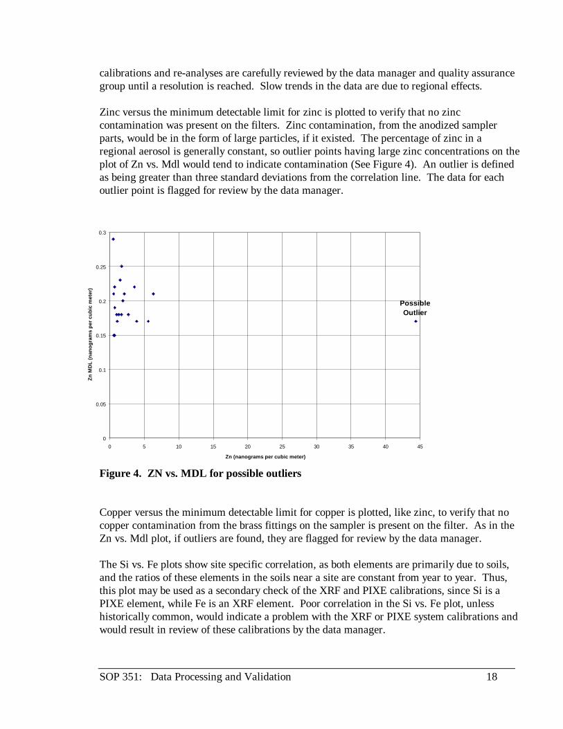
Zinc versus the minimum detectable limit for zinc is plotted to verify that no zinccontamination was present on the filters. Zinc contamination, from the anodized samplerparts, would be in the form of large particles, if it existed. The percentage of zinc in aregional aerosol is generally constant, so outlier points having large zinc concentrations on theplot of Zn vs. Mdl would tend to indicate contamination (See Figure 4). An outlier is definedas being greater than three standard deviations from the correlation line. The data for eachoutlier point is flagged for review by the data manager.
Figure 4. ZN vs. MDL for possible outliers
Copper versus the minimum detectable limit for copper is plotted, like zinc, to verify that nocopper contamination from the brass fittings on the sampler is present on the filter. As in theZn vs. Mdl plot, if outliers are found, they are flagged for review by the data manager.
The Si vs. Fe plots show site specific correlation, as both elements are primarily due to soils,and the ratios of these elements in the soils near a site are constant from year to year. Thus,this plot may be used as a secondary check of the XRF and PIXE calibrations, since Si is aPIXE element, while Fe is an XRF element. Poor correlation in the Si vs. Fe plot, unlesshistorically common, would indicate a problem with the XRF or PIXE system calibrations andwould result in review of these calibrations by the data manager.
PossibleOutlier
0
0.05
0.1
0.15
0.2
0.25
0.3
0 5 10 15 20 25 30 35 40 45
Zn (nanograms per cubic meter)
Zn M
DL
(nan
ogra
ms
per
cubi
c m
eter
)
SOP 351: Data Processing and Validation 19
The gravimetric mass versus H plot is meant to prove that PESA data was collected for all thesamples. The plot also verifies the functioning of the PESA system since the ratio of organicmatter to fine mass is roughly constant at four to five percent. Higher or lower ratios mayindicate improper calibration of the PESA system, or invalid gravimetric mass data.
The gravimetric mass versus reconstructed mass plot is done as further quality assurance ofthe gravimetric data. Reconstructed mass, RCMA, is generated from data collected duringanalysis and does not include organic or nitrate contributions to the measured mass. RCMAgenerally correlates well with the fine gravimetric mass, MF, and stray data points aretypically due to invalid gravimetric mass data. The measured and reconstructed mass shouldcorrelate well, with the reconstructed mass being between 85% and 100% of the measuredmass. The percentage is site dependent and is generally reflected in historical data. If thepercentage is substantially different from past values, or is out of range, there may be aproblem with the sampler or the elemental analysis. The sampler flow, the sample duration,and the deposit area would be carefully verified, as well as the calibration values and re-analysis data from the PIXE run until the data were resolved. Invalid gravimetric data wouldbe flagged for deletion.
4.2.3.4 Quality assurance of flow rate data
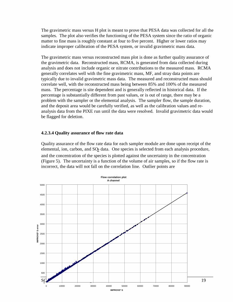
Quality assurance of the flow rate data for each sampler module are done upon receipt of theelemental, ion, carbon, and SO2 data. One species is selected from each analysis procedure,and the concentration of the species is plotted against the uncertainty in the concentration(Figure 5). The uncertainty is a function of the volume of air samples, so if the flow rate isincorrect, the data will not fall on the correlation line. Outlier points are
Flow correlation plotA channel
0
500
1000
1500
2000
2500
3000
3500
4000
4500
5000
0 10000 20000 30000 40000 50000 60000 70000 80000 90000
IMPROVE* S
IMP
RO
VE
* S
err
or
SOP 351: Data Processing and Validation 20
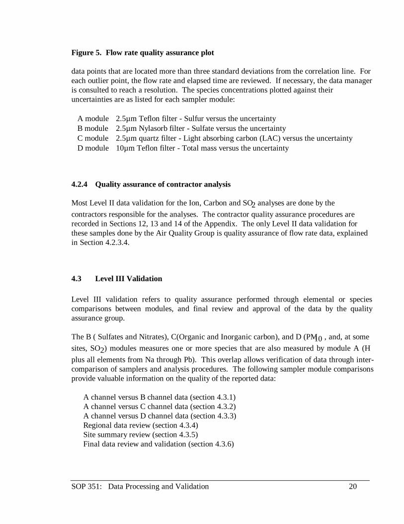
Figure 5. Flow rate quality assurance plot
data points that are located more than three standard deviations from the correlation line. Foreach outlier point, the flow rate and elapsed time are reviewed. If necessary, the data manageris consulted to reach a resolution. The species concentrations plotted against theiruncertainties are as listed for each sampler module:
A module 2.5µm Teflon filter - Sulfur versus the uncertaintyB module 2.5µm Nylasorb filter - Sulfate versus the uncertaintyC module 2.5µm quartz filter - Light absorbing carbon (LAC) versus the uncertaintyD module 10µm Teflon filter - Total mass versus the uncertainty
4.2.4 Quality assurance of contractor analysis
Most Level II data validation for the Ion, Carbon and SO2 analyses are done by thecontractors responsible for the analyses. The contractor quality assurance procedures arerecorded in Sections 12, 13 and 14 of the Appendix. The only Level II data validation forthese samples done by the Air Quality Group is quality assurance of flow rate data, explainedin Section 4.2.3.4.
4.3 Level III Validation
Level III validation refers to quality assurance performed through elemental or speciescomparisons between modules, and final review and approval of the data by the qualityassurance group.
The B ( Sulfates and Nitrates), C(Organic and Inorganic carbon), and D (PM10 , and, at somesites, SO2) modules measures one or more species that are also measured by module A (Hplus all elements from Na through Pb). This overlap allows verification of data through inter-comparison of samplers and analysis procedures. The following sampler module comparisonsprovide valuable information on the quality of the reported data:
A channel versus B channel data (section 4.3.1)A channel versus C channel data (section 4.3.2)A channel versus D channel data (section 4.3.3)Regional data review (section 4.3.4)Site summary review (section 4.3.5)Final data review and validation (section 4.3.6)

SOP 351: Data Processing and Validation 21
4.3.1 A channel versus B channel data
Quality assurance for the A and B modules consists of comparison of the measuredconcentration of sulfur and sulfate (See Figure 6). Sulfur concentrations are reported throughelemental analysis, while sulfate concentrations are derived through ion chromatographyanalysis. Since both modules sample simultaneously and have the same flow and aerosol sizecut point, the collected data should correlate.
Any data more than three standard deviations from the correlation line are considered to beoutlier points. All outlier points are carefully reviewed for flow rate entry errors, or analyticalerrors. Corrections are made and unresolved outlier data are flagged for review by the datamanager and quality assurance group.
Figure 6. Elemental Sulfur vs. Ionic Sulfate
4.3.2 A channel versus C channel data
B96TOT, N = 1340, R = 0.996, R^2 = 0.991Y = 1.0009*X + (-47.7366), Slope error = 0.004, Intcpt. error = 15.459
Mean X = 2624.55, Error = 90.68, Std Dev. = 3319.47Mean Y = 2579.09, Error = 90.76, Std Dev. = 3322.33
Mean Y/Mean X = 0.983
0
5000
10000
15000
20000
25000
0 5000 10000 15000 20000 25000
IMPROVE* S3
IMP
RO
VE
* S
O4
SOP 351: Data Processing and Validation 22
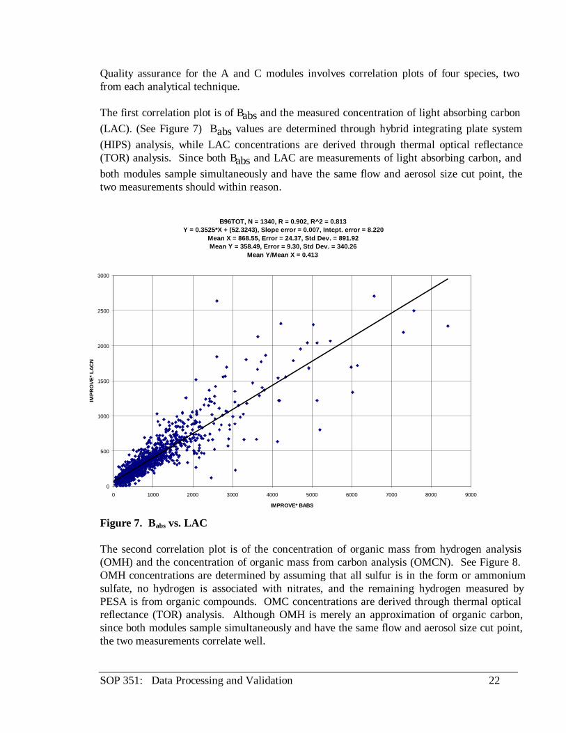
Quality assurance for the A and C modules involves correlation plots of four species, twofrom each analytical technique.
The first correlation plot is of Babs and the measured concentration of light absorbing carbon(LAC). (See Figure 7) Babs values are determined through hybrid integrating plate system(HIPS) analysis, while LAC concentrations are derived through thermal optical reflectance(TOR) analysis. Since both Babs and LAC are measurements of light absorbing carbon, andboth modules sample simultaneously and have the same flow and aerosol size cut point, thetwo measurements should within reason.
Figure 7. Babs vs. LAC
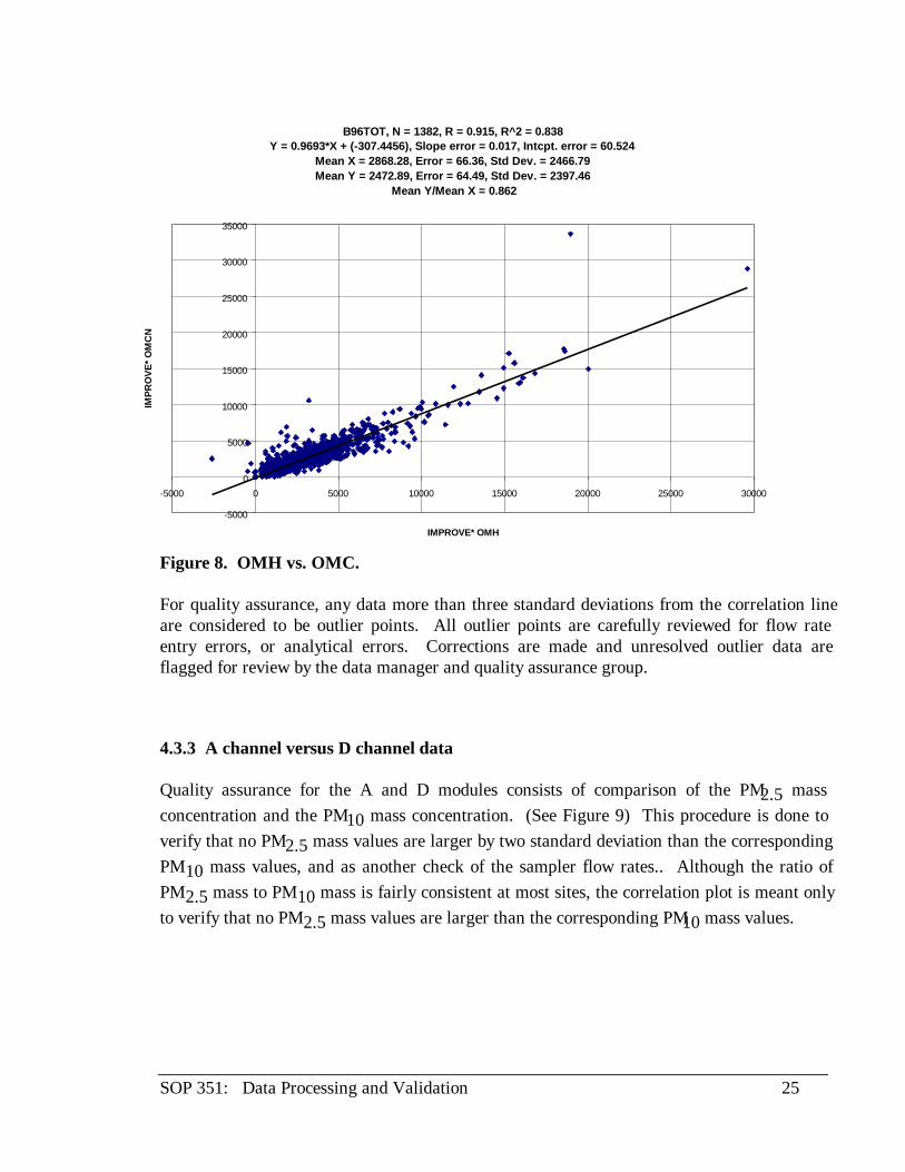
The second correlation plot is of the concentration of organic mass from hydrogen analysis(OMH) and the concentration of organic mass from carbon analysis (OMCN). See Figure 8.OMH concentrations are determined by assuming that all sulfur is in the form or ammoniumsulfate, no hydrogen is associated with nitrates, and the remaining hydrogen measured byPESA is from organic compounds. OMC concentrations are derived through thermal opticalreflectance (TOR) analysis. Although OMH is merely an approximation of organic carbon,since both modules sample simultaneously and have the same flow and aerosol size cut point,the two measurements correlate well.
B96TOT, N = 1340, R = 0.902, R^2 = 0.813Y = 0.3525*X + (52.3243), Slope error = 0.007, Intcpt. error = 8.220
Mean X = 868.55, Error = 24.37, Std Dev. = 891.92Mean Y = 358.49, Error = 9.30, Std Dev. = 340.26
Mean Y/Mean X = 0.413
0
500
1000
1500
2000
2500
3000
0 1000 2000 3000 4000 5000 6000 7000 8000 9000
IMPROVE* BABS
IMP
RO
VE
* LA
CN

SOP 351: Data Processing and Validation 23
Figure 6. Elemental Sulfur vs. Ionic Sulfate
4.3.2 A channel versus C channel data
Quality assurance for the A and C modules involves correlation plots of four species, twofrom each analytical technique.
The first correlation plot is of Babs and the measured concentration of light absorbing carbon(LAC). (See Figure 7) Babs values are determined through hybrid integrating plate system(HIPS) analysis, while LAC concentrations are derived through thermal optical reflectance(TOR) analysis. Since both Babs and LAC are measurements of light absorbing carbon, andboth modules sample simultaneously and have the same flow and aerosol size cut point, thetwo measurements should within reason.
B96TOT, N = 1340, R = 0.996, R^2 = 0.991Y = 1.0009*X + (-47.7366), Slope error = 0.004, Intcpt. error = 15.459
Mean X = 2624.55, Error = 90.68, Std Dev. = 3319.47Mean Y = 2579.09, Error = 90.76, Std Dev. = 3322.33
Mean Y/Mean X = 0.983
0
5000
10000
15000
20000
25000
0 5000 10000 15000 20000 25000
IMPROVE* S3
IMP
RO
VE
* S
O4

SOP 351: Data Processing and Validation 24
Figure 7. Babs vs. LAC
The second correlation plot is of the concentration of organic mass from hydrogen analysis(OMH) and the concentration of organic mass from carbon analysis (OMCN). See Figure 8.OMH concentrations are determined by assuming that all sulfur is in the form or ammoniumsulfate, no hydrogen is associated with nitrates, and the remaining hydrogen measured byPESA is from organic compounds. OMC concentrations are derived through thermal opticalreflectance (TOR) analysis. Although OMH is merely an approximation of organic carbon,since both modules sample simultaneously and have the same flow and aerosol size cut point,the two measurements correlate well.
B96TOT, N = 1340, R = 0.902, R^2 = 0.813Y = 0.3525*X + (52.3243), Slope error = 0.007, Intcpt. error = 8.220
Mean X = 868.55, Error = 24.37, Std Dev. = 891.92Mean Y = 358.49, Error = 9.30, Std Dev. = 340.26
Mean Y/Mean X = 0.413
0
500
1000
1500
2000
2500
3000
0 1000 2000 3000 4000 5000 6000 7000 8000 9000
IMPROVE* BABS
IMP
RO
VE
* LA
CN
SOP 351: Data Processing and Validation 25
Figure 8. OMH vs. OMC.
For quality assurance, any data more than three standard deviations from the correlation lineare considered to be outlier points. All outlier points are carefully reviewed for flow rateentry errors, or analytical errors. Corrections are made and unresolved outlier data areflagged for review by the data manager and quality assurance group.
4.3.3 A channel versus D channel data
Quality assurance for the A and D modules consists of comparison of the PM2.5 massconcentration and the PM10 mass concentration. (See Figure 9) This procedure is done toverify that no PM2.5 mass values are larger by two standard deviation than the correspondingPM10 mass values, and as another check of the sampler flow rates.. Although the ratio ofPM2.5 mass to PM10 mass is fairly consistent at most sites, the correlation plot is meant onlyto verify that no PM2.5 mass values are larger than the corresponding PM10 mass values.
B96TOT, N = 1382, R = 0.915, R^2 = 0.838Y = 0.9693*X + (-307.4456), Slope error = 0.017, Intcpt. error = 60.524
Mean X = 2868.28, Error = 66.36, Std Dev. = 2466.79Mean Y = 2472.89, Error = 64.49, Std Dev. = 2397.46
Mean Y/Mean X = 0.862
-5000
0
5000
10000
15000
20000
25000
30000
35000
-5000 0 5000 10000 15000 20000 25000 30000
IMPROVE* OMH
IMP
RO
VE
* O
MC
N

IMPROVE Network Standard Operating Procedures
Section 351: Data Processing and Validation 26
Figure 9. MF vs. MT
4.3.4 Regional data review
Most sites in the IMPROVE network fall into one of two groups, according the samplingconditions and the historical data.
The Eastern sites are those which historically have high humidity in the summer, are East ofthe Mississippi River, have relatively larger mass loadings, and proportionally higher sulfurconcentrations.
The Western sites are those which historically have low humidity, are west of the MississippiRiver, have relatively lower mass loadings, and proportionally higher soil concentrations.
Sites not included in this group are included in the All Sites group, though this grouping is lesseffective for quality assurance than the Eastern or Western groups.
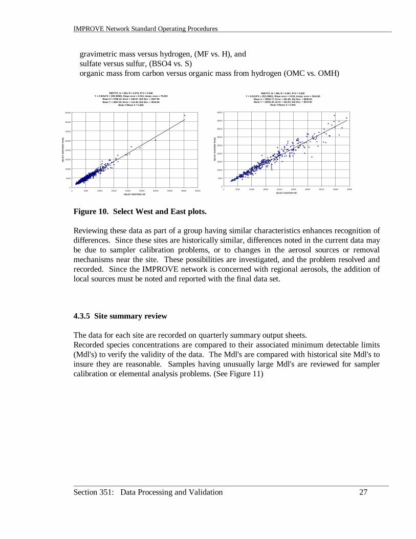
For each group, Eastern, Western, and All Sites, the following correlation plots are created:gravimetric mass versus reconstructed mass,(MF vs. RCMA - See Figure 10),
B96TOT, N = 1365, R = 0.860, R^2 = 0.740Y = 1.3973*X + (2864.5045), Slope error = 0.033, Intcpt. error = 361.599
Mean X = 9034.26, Error = 198.33, Std Dev. = 7327.46Mean Y = 15488.18, Error = 264.80, Std Dev. = 9783.34
Mean Y/Mean X = 1.714
0
10000
20000
30000
40000
50000
60000
0 5000 10000 15000 20000 25000 30000 35000 40000 45000 50000
IMPROVE* MF
IMP
RO
VE
* M
T
IMPROVE Network Standard Operating Procedures
Section 351: Data Processing and Validation 27
gravimetric mass versus hydrogen, (MF vs. H), andsulfate versus sulfur, (BSO4 vs. S)organic mass from carbon versus organic mass from hydrogen (OMC vs. OMH)
Figure 10. Select West and East plots.
Reviewing these data as part of a group having similar characteristics enhances recognition ofdifferences. Since these sites are historically similar, differences noted in the current data maybe due to sampler calibration problems, or to changes in the aerosol sources or removalmechanisms near the site. These possibilities are investigated, and the problem resolved andrecorded. Since the IMPROVE network is concerned with regional aerosols, the addition oflocal sources must be noted and reported with the final data set.
4.3.5 Site summary review
The data for each site are recorded on quarterly summary output sheets.Recorded species concentrations are compared to their associated minimum detectable limits(Mdl's) to verify the validity of the data. The Mdl's are compared with historical site Mdl's toinsure they are reasonable. Samples having unusually large Mdl's are reviewed for samplercalibration or elemental analysis problems. (See Figure 11)
B96TOT, N = 366, R = 0.967, R^2 = 0.935Y = 0.9110*X + (521.8891), Slope error = 0.018, Intcpt. error = 324.292
Mean X = 15992.17, Error = 461.85, Std Dev. = 8835.63Mean Y = 15091.05, Error = 422.03, Std Dev. = 8074.00
Mean Y/Mean X = 0.944
0
5000
10000
15000
20000
25000
30000
35000
40000
45000
0 5000 10000 15000 20000 25000 30000 35000 40000 45000
SELECT EASTERN* MF
SE
LEC
T E
AS
TER
N*
RC
MA
B96TOT, N = 694, R = 0.974, R^2 = 0.948Y = 0.9014*X + (391.8582), Slope error = 0.011, Intcpt. error = 75.633
Mean X = 5786.12, Error = 126.67, Std Dev. = 3337.06Mean Y = 5607.22, Error = 114.49, Std Dev. = 3016.06
Mean Y/Mean X = 0.969
0
5000
10000
15000
20000
25000
30000
35000
40000
0 5000 10000 15000 20000 25000 30000 35000 40000 45000
SELECT WESTERN* MF
SE
LEC
T W
ES
TER
N*
RC
MA

IMPROVE Network Standard Operating Procedures
Section 351: Data Processing and Validation 28
Finally, all missing data is noted and flagged for verification of invalid status.
4.3.6 Final data review and validation
Once all data corrections have been entered, and the data have been processed to their finalform, the archived information for the quarter is submitted to the quality assurance group.Any remaining problems are resolved, and the final data set is agreed upon.
S e M D L i n n a n o g r a m s p e r c u b i c m e t e r
0
0 . 0 1
0 . 0 2
0 . 0 3
0 . 0 4
0 . 0 5
0 . 0 6
0 . 0 7
0 . 0 8
3/1/
95
3/11
/95
3/22
/95
4/1/
95
4/12
/95
4/22
/95
5/3/
95
5/13
/95
5/24
/95
6/3/
95
6/14
/95
6/24
/95
7/5/
95
7/15
/95
7/26
/95
8/5/
95
8/16
/95
8/26
/95
9/9/
95
9/20
/95
9/30
/95
10/1
1/95
10/2
1/95
11/1
/95
11/1
1/95
11/2
2/95
12/2
/95
12/1
3/95
1/17
/96
1/27
/96
2/7/
96
2/17
/96
2/28
/96
Se
MD
L in
nan
ogra
ms
per
cubi
c m
eter
S e _ M D L
Figure 11. MDL plot

IMPROVE Network Standard Operating Procedures
Section 351: Data Processing and Validation 29
4.4 Modification and Documentation of Parameters
All parameters in any database that are changed are logged into the computer. Theparameters can be changed only by restricted programs. Access to these programs are limitedto key personnel, including the QA manager. The main program that has the ability to modifythe IMPROVE databases is called Auxdata. Auxdata is a versatile program that allows theQA manager/specialists to view and/or edit the aerosol databases. The main screen displaysthe status of each of the samples and gives a menu of functions such as editing andbackground analysis. (See Figure 10) This interface allows access to all the databasesreferred in SOP 251. Following the procedures outlined earlier in this document, the user mayhave the need to modify the databases. Auxdata is the only program that will allow changesto databases.
In addition to edits, the program creates several files for additional quality assurance and foruse by end users here at UCD. These files can be used by other programs created by the enduser for reports or other statistical analysis.
F1 = WriteACAD1 A96 MT MF LRNC H 3*S SO4 FE O3 SO2 F1 = Write Auxfile F2 = Change Season F3 = Exit Code F8 = Efficiency&Ctrls F9 = Write The Rest F10 = Edit Databases F11 = Write Replicates F12 = Check Files Shift+F2 = Total DBF Shift+F3 = View Problems PGUP=Last Site/NoWRITE PGDN=Next Site/No WRITE
SO2=2.42±0.48 N=8 F5=Det IONS Art. N=26 F6=Details CL =0.21±0.14 NO2=0.27±.17 NO3=0.59±0.11 SO4=0.48±.27 Carb Art. N=94 F7=Details O1 =3.40±1.6 02 =2.80±1.5 O3 =3.70±1.1 O4 =1.10±.43 OP =0.00±.35 E1 =0.30±.39 E2 =1.30±.57 E3 =0.30±.35
03/02/96 0000 15 6 443 0.2 2.4 2.1 16 0.2 2.603/06/96 0000 14 8 479 0.3 4.2 0 16 0.2 2.203/09/96 0000 6 4 228 0.1 1.7 0 12 0.2 1.103/13/96 0000 18 9 557 0.4 4.5 4.1 43 0.3 5.003/16/96 0000 6 4 210 0.1 1.6 1.4 11 0.2 0.503/20/96 0000 9 3 171 0.1 1.1 1.0 19 0.1 0.803/23/96 0000 8 4 268 0.2 1.9 1.7 8 0.1 0.403/27/96 0000 17 3 180 0.1 1.7 1.5 22 0.1 1.103/30/96 0000 6 3 198 0.1 1.8 1.5 25 0.1 1.104/03/96 0000 8 3 149 0.1 1.7 1.7 24 0.0 0.504/06/96 0000 10 5 144 0.1 1.7 1.4 11 0.1 0.704/10/96 0000 1 1 81 0.0 0.4 0.4 1 0.0 0.104/13/96 0000 4 2 177 0.1 1.1 1.0 12 0.1 0.504/17/96 0000 11 6 240 0.1 1.9 1.7 7 0.1 0.304/20/96 0000 16 10 546 0.4 4.8 4.6 29 0.2 0.604/24/96 0000 8 3 105 0.1 1.6 1.4 5 0.0 0.104/27/96 0000 10 6 249 0.2 2.7 2.6 14 0.1 0.405/01/96 0000 6 3 127 0.2 1.7 1.5 10 0.0 0.105/04/96 0000 9 7 390 0.3 4.1 3.7 8 0.0 0.605/08/96 0000 10 4 410 0.1 1.2 1.1 23 0.2 1.605/11/96 0000 3 1 106 0.0 0.5 0.4 1 0.0 0.005/14/96 0000 11 7 492 0.3 3.5 3.3 25 0.2 1.205/18/96 0000 3 1 90 0.0 0.8 0.6 2 0.1 0.205/22/96 0000 10 5 283 0.1 1.2 1.0 16 0.2 0.2
Figure 10. Auxdata Main Screen
IMPROVE Network Standard Operating Procedures
Section 351: Data Processing and Validation 30
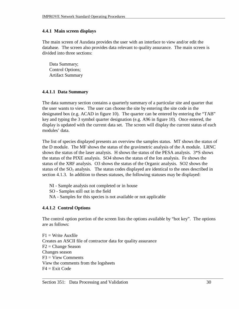
4.4.1 Main screen displays
The main screen of Auxdata provides the user with an interface to view and/or edit thedatabase. The screen also provides data relevant to quality assurance. The main screen isdivided into three sections:
Data Summary;Control Options;Artifact Summary
4.4.1.1 Data Summary
The data summary section contains a quarterly summary of a particular site and quarter thatthe user wants to view. The user can choose the site by entering the site code in thedesignated box (e.g. ACAD in figure 10). The quarter can be entered by entering the “TAB”key and typing the 3 symbol quarter designation (e.g. A96 in figure 10). Once entered, thedisplay is updated with the current data set. The screen will display the current status of eachmodules’ data.
The list of species displayed presents an overview the samples status. MT shows the status ofthe D module. The MF shows the status of the gravimetric analysis of the A module. LRNCshows the status of the laser analysis. H shows the status of the PESA analysis. 3*S showsthe status of the PIXE analysis. SO4 shows the status of the Ion analysis. Fe shows thestatus of the XRF analysis. O3 shows the status of the Organic analysis. SO2 shows thestatus of the SO2 analysis. The status codes displayed are identical to the ones described insection 4.1.3. In addition to theses statuses, the following statuses may be displayed:
NI - Sample analysis not completed or in houseSO - Samples still out in the fieldNA - Samples for this species is not available or not applicable
4.4.1.2 Control Options
The control option portion of the screen lists the options available by “hot key”. The optionsare as follows:
F1 = Write AuxfileCreates an ASCII file of contractor data for quality assuranceF2 = Change SeasonChanges seasonF3 = View CommentsView the comments from the logsheetsF4 = Exit Code

IMPROVE Network Standard Operating Procedures
Section 351: Data Processing and Validation 31
Exit codeF8 = Efficiency&CtrlsShows a table of the number of samples collected and laboratory controls.F9 = Write The RestWrites the rest of the Auxfiles starting with the site outputted on the screen and workingdown alphabeticallyF10 = Edit DatabasesAllows user to edit the databasesF11 = Write ReplicatesProduces a summary of all samples that are reanalyzed and compares to the originalF12 = Check FilesCheck files for duplications, deletes and other abnormalitiesShift+F2 = Total DBFCreates a single database for quality assurance testsShift+F3 = View ProblemsViews a problem file that records any past problems from that particular sitePGUP=Last Site/NoWRITEMoves up to the next sitePGDN=Next Site/NoWRITEMoves down to the next site.
4.4.1.3 Artifact Summary
The portion of the screen displays the artifact or blank subtraction from the variouscontractors. They included SO2, ions and carbon analysis. The numbers are based on fieldblanks taken during the quarter of analysis.
4.4.2 Subscreens
This option is still under construction and is meant to enhance the viewing of the IMPROVEdatabase. This may included other graphical or textual representation of the data set.
IMPROVE Network Standard Operating Procedures
Section 351: Data Processing and Validation 32
4.5 Calculations
This section deals with the equations used to determine the various derived parameters. Theyare given in the following sections:
Flow Equations (4.5.1);Determination of Concentration, Artifact, and Precision (4.5.2);Equations of Composite Variable (4.5.3).
4.5.1 Flow Equations
The following section derives equations used to determine the flow rate and other aspects ofaerosol sampling. This section is divided in the following manner:
The Effect of Flow Rate on Cyclone Cut Point (4.5.1.1);Flow Control by a Critical Orifice (4.5.1.2);Flow Rate through an Orifice Meter (4.5.1.3);Pressure-Elevation Relationships (4.5.1.4);Calibration of Audit Devices (4.5.1.5);Nominal Flow Rate Equation (4.5.1.6);Flow Rate Equations for the System Vacuum Gauge (4.5.1.7);Calibration of the System Orifice Meter and Vacuum Gauge (4.5.1.8)
4.5.1.1 The Effect of Flow Rate on Cyclone Cut Point
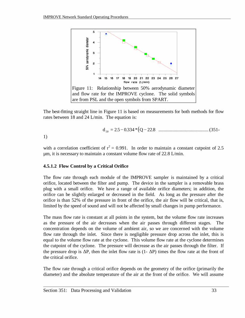
The collection efficiency of the IMPROVE cyclone was characterized at the Health SciencesInstrumentation Facility at the University of California at Davis. The efficiency was measuredas a function of particle size and flow rate using two separate methods: PSL and SPART.Both use microspheres of fluorescent polystyrene latex particles (PSL) produced by aLovelace nebulizer and a vibrating stream generator. The PSL method analyzed these byelectron micrographs, while the SPART method analyzed them by a Single ParticleAerodynamic Relaxation Time analyzer. The aerodynamic diameter for 50% collection, d50,was determined for each flow rate. The relationship between diameter and flow rate is shownin Figure 11.
IMPROVE Network Standard Operating Procedures
Section 351: Data Processing and Validation 33
Figure 11: Relationship between 50% aerodynamic diameterand flow rate for the IMPROVE cyclone. The solid symbolsare from PSL and the open symbols from SPART.
The best-fitting straight line in Figure 11 is based on measurements for both methods for flowrates between 18 and 24 L/min. The equation is:
( )d Q50 2 5 0 334 22 8= − −. . * . ........................................ (351-1)
with a correlation coefficient of r2 = 0.991. In order to maintain a constant cutpoint of 2.5µm, it is necessary to maintain a constant volume flow rate of 22.8 L/min.
4.5.1.2 Flow Control by a Critical Orifice
The flow rate through each module of the IMPROVE sampler is maintained by a criticalorifice, located between the filter and pump. The device in the sampler is a removable brassplug with a small orifice. We have a range of available orifice diameters; in addition, theorifice can be slightly enlarged or decreased in the field. As long as the pressure after theorifice is than 52% of the pressure in front of the orifice, the air flow will be critical, that is,limited by the speed of sound and will not be affected by small changes in pump performance.
The mass flow rate is constant at all points in the system, but the volume flow rate increasesas the pressure of the air decreases when the air passes through different stages. Theconcentration depends on the volume of ambient air, so we are concerned with the volumeflow rate through the inlet. Since there is negligible pressure drop across the inlet, this isequal to the volume flow rate at the cyclone. This volume flow rate at the cyclone determinesthe cutpoint of the cyclone. The pressure will decrease as the air passes through the filter. Ifthe pressure drop is ∆P, then the inlet flow rate is (1- ∆P) times the flow rate at the front ofthe critical orifice.
The flow rate through a critical orifice depends on the geometry of the orifice (primarily thediameter) and the absolute temperature of the air at the front of the orifice. We will assume
IMPROVE Network Standard Operating Procedures
Section 351: Data Processing and Validation 34
that this temperature is the same as the ambient temperature. The flow rate at the criticalorifice differs from the inlet flow rate because of the pressure drop as the air passes throughthe filter. We have chosen to express all calibrations relative to a common temperature, 20°C.The equation for the inlet flow rate is
Q = Qo * 1 −
∆PP
* T + 273293
, (351-2)
where Qo is a constant and ∆P/P is the relative decrease in pressure before the orifice. Thepressure drop ∆P is produced primarily by the filter, either because of the pressure drop of aclean filter or because of filter loading. To account for the pressure drop of the clean filter,each critical orifice is adjusted during calibration to give the desired flow rate with a typicalclean filter appropriate for the module. The important pressure quantity is the variation, δP,about the nominal pressure drop of the clean filter used in calibration, ∆Pnom:
δP = ∆Pnom - ∆P .................................................. (351-3)
If δP is associated with variation in the clean filter, it can be either negative or positive, andwill affect the measurements before and after collection equally. If the variation is caused byfilter loading; δP will be positive and affect only the final flow rate measurement. For thisreason we average the two readings.
The annual mean temperatures for all the IMPROVE sites, based on the weekly temperaturemeasurements is 15°C. In order to have the mean annual flow rate at 22.8 L/min, the criticalorifices are adjusted to provide a flow rate of 23 L/min at 20°C with a typical filter in thecassette. The constant Qo in Equation 351-2 is then given by
Qo = 23.0 * 11
−
−∆PPnom ,......................................... (351-
4)
The nominal flow rate is set at 19.1 L/min at 20°C for the Wedding PM10 inlet, and at 17.8L/min for the Sierra-Anderson PM10 inlet.
Substituting Equation 351-4 into Equation 351-2, and assuming there is no variation inatmospheric pressure at the site, the flow rate is given by
Q = 23.0 * 1 − −
δPP Pnom∆ * T + 273
293 , .............................. (351-
5)
Effect of Temperature and Pressure Drop on Cyclone Efficiency
IMPROVE Network Standard Operating Procedures
Section 351: Data Processing and Validation 35
Variations in temperature with site and season affect the collection cut point but not thevolume calculation. The mean annual d50 will be slightly lower at warm sites than at cold.Saguaro (22°C) would have an annual d50 of 2.4 µm, while Denali (2°C) would have a d50 of2.7 µm. For a given site, the mean d50 in summer will be lower than in winter. For example,based on historical records, the d50 at Davis would vary between 2.4 µm in midsummer and2.6 µm in midwinter. At the highest maximum temperature recorded at Davis (34°C), the d50
would drop to 2.2 µm.
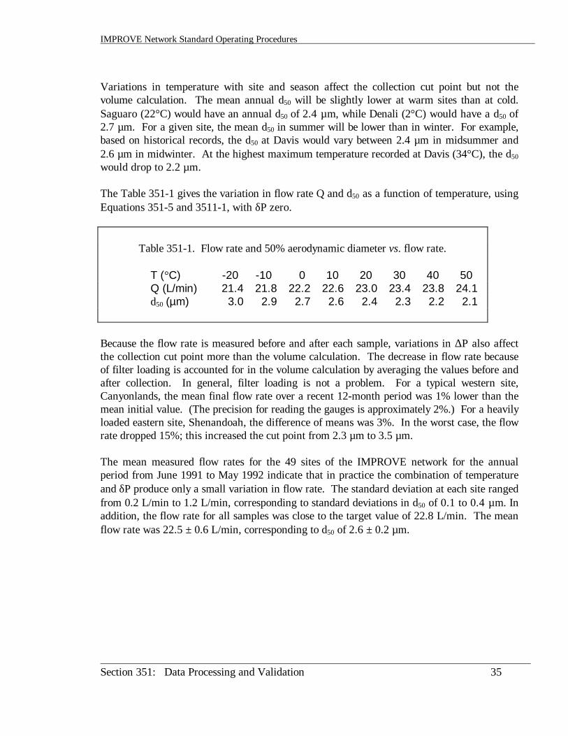
The Table 351-1 gives the variation in flow rate Q and d50 as a function of temperature, usingEquations 351-5 and 3511-1, with δP zero.
Table 351-1. Flow rate and 50% aerodynamic diameter vs. flow rate.
T (°C) -20 -10 0 10 20 30 40 50Q (L/min) 21.4 21.8 22.2 22.6 23.0 23.4 23.8 24.1d50 (µm) 3.0 2.9 2.7 2.6 2.4 2.3 2.2 2.1
Because the flow rate is measured before and after each sample, variations in ∆P also affectthe collection cut point more than the volume calculation. The decrease in flow rate becauseof filter loading is accounted for in the volume calculation by averaging the values before andafter collection. In general, filter loading is not a problem. For a typical western site,Canyonlands, the mean final flow rate over a recent 12-month period was 1% lower than themean initial value. (The precision for reading the gauges is approximately 2%.) For a heavilyloaded eastern site, Shenandoah, the difference of means was 3%. In the worst case, the flowrate dropped 15%; this increased the cut point from 2.3 µm to 3.5 µm.
The mean measured flow rates for the 49 sites of the IMPROVE network for the annualperiod from June 1991 to May 1992 indicate that in practice the combination of temperatureand δP produce only a small variation in flow rate. The standard deviation at each site rangedfrom 0.2 L/min to 1.2 L/min, corresponding to standard deviations in d50 of 0.1 to 0.4 µm. Inaddition, the flow rate for all samples was close to the target value of 22.8 L/min. The meanflow rate was 22.5 ± 0.6 L/min, corresponding to d50 of 2.6 ± 0.2 µm.
IMPROVE Network Standard Operating Procedures
Section 351: Data Processing and Validation 36
Effect of Temperature and Pressure Drop on the Volume Calculation
The major error in volume calculation would occur when the mean temperature for a 24-hoursample differs significantly from the mean temperature of the two readings during the samplechanges. Normally this is not a significant problem, but could occasionally occur. Adifference of 5°C would produce an error of 1%, while a 10°C difference would produce anerror of 2%.
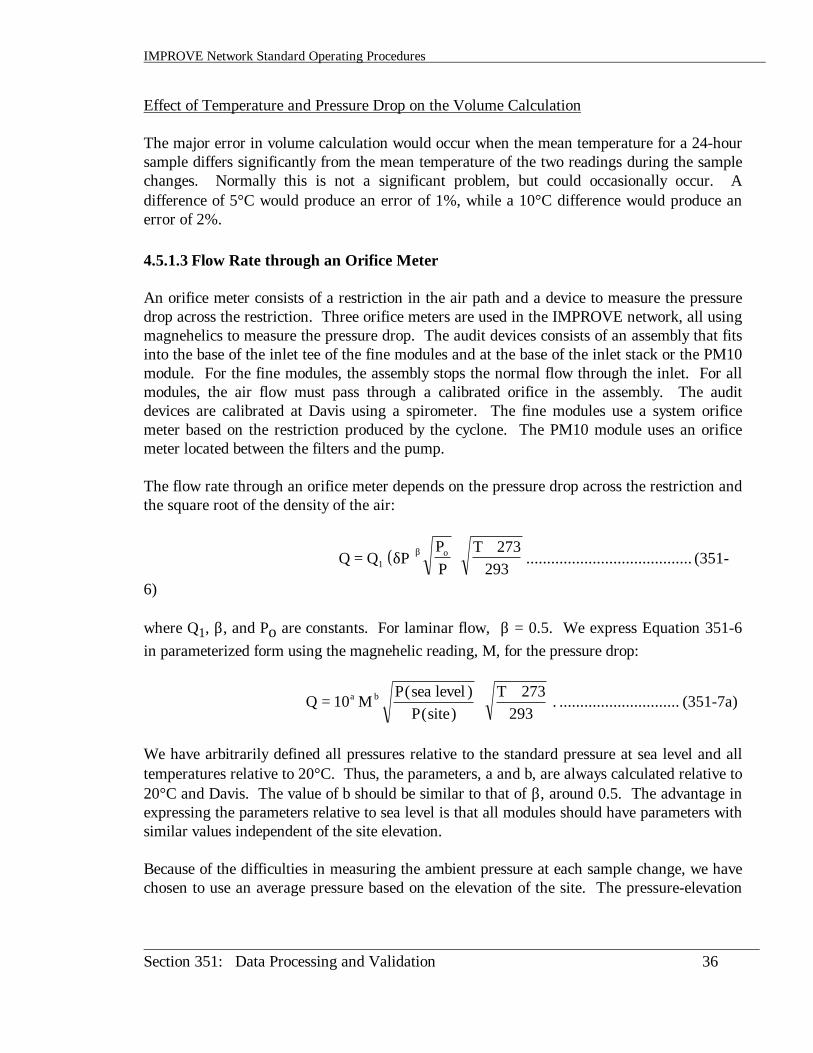
4.5.1.3 Flow Rate through an Orifice Meter
An orifice meter consists of a restriction in the air path and a device to measure the pressuredrop across the restriction. Three orifice meters are used in the IMPROVE network, all usingmagnehelics to measure the pressure drop. The audit devices consists of an assembly that fitsinto the base of the inlet tee of the fine modules and at the base of the inlet stack or the PM10module. For the fine modules, the assembly stops the normal flow through the inlet. For allmodules, the air flow must pass through a calibrated orifice in the assembly. The auditdevices are calibrated at Davis using a spirometer. The fine modules use a system orificemeter based on the restriction produced by the cyclone. The PM10 module uses an orificemeter located between the filters and the pump.
The flow rate through an orifice meter depends on the pressure drop across the restriction andthe square root of the density of the air:
( )Q Q PPP
To= +1
273293
δ β ........................................ (351-
6)
where Q1, β, and Po are constants. For laminar flow, β = 0.5. We express Equation 351-6in parameterized form using the magnehelic reading, M, for the pressure drop:
Q MP
P siteTa b= +
10273
293( )
( )sea level
. ............................. (351-7a)
We have arbitrarily defined all pressures relative to the standard pressure at sea level and alltemperatures relative to 20°C. Thus, the parameters, a and b, are always calculated relative to20°C and Davis. The value of b should be similar to that of β, around 0.5. The advantage inexpressing the parameters relative to sea level is that all modules should have parameters withsimilar values independent of the site elevation.
Because of the difficulties in measuring the ambient pressure at each sample change, we havechosen to use an average pressure based on the elevation of the site. The pressure-elevation
IMPROVE Network Standard Operating Procedures
Section 351: Data Processing and Validation 37
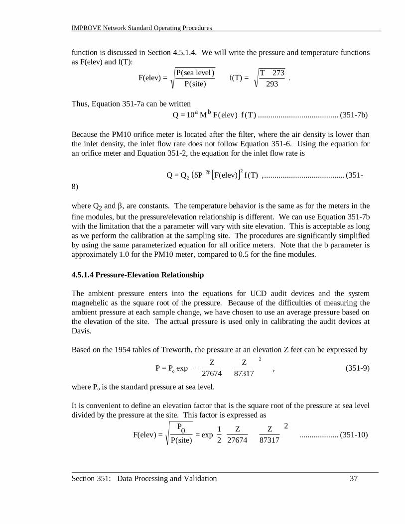
function is discussed in Section 4.5.1.4. We will write the pressure and temperature functionsas F(elev) and f(T):
F(elev) = P
P site( )
( )sea level
f(T) = T + 273293
.
Thus, Equation 351-7a can be writtenQ M F elev f Ta b= 10 ( ) ( ) ....................................... (351-7b)
Because the PM10 orifice meter is located after the filter, where the air density is lower thanthe inlet density, the inlet flow rate does not follow Equation 351-6. Using the equation foran orifice meter and Equation 351-2, the equation for the inlet flow rate is
( ) [ ]Q Q P F elev f T= 22 2δ β ( ) ( ) ,....................................... (351-
8)
where Q2 and β, are constants. The temperature behavior is the same as for the meters in thefine modules, but the pressure/elevation relationship is different. We can use Equation 351-7bwith the limitation that the a parameter will vary with site elevation. This is acceptable as longas we perform the calibration at the sampling site. The procedures are significantly simplifiedby using the same parameterized equation for all orifice meters. Note that the b parameter isapproximately 1.0 for the PM10 meter, compared to 0.5 for the fine modules.
4.5.1.4 Pressure-Elevation Relationship
The ambient pressure enters into the equations for UCD audit devices and the systemmagnehelic as the square root of the pressure. Because of the difficulties of measuring theambient pressure at each sample change, we have chosen to use an average pressure based onthe elevation of the site. The actual pressure is used only in calibrating the audit devices atDavis.
Based on the 1954 tables of Treworth, the pressure at an elevation Z feet can be expressed by
P PZ Z
o= − +
exp27674 87317
2
, (351-9)
where Po is the standard pressure at sea level.
It is convenient to define an elevation factor that is the square root of the pressure at sea leveldivided by the pressure at the site. This factor is expressed as
F elevP
P siteZ Z
( )( )
exp= = +
0 12 27674 87317
2................... (351-10)

IMPROVE Network Standard Operating Procedures
Section 351: Data Processing and Validation 38
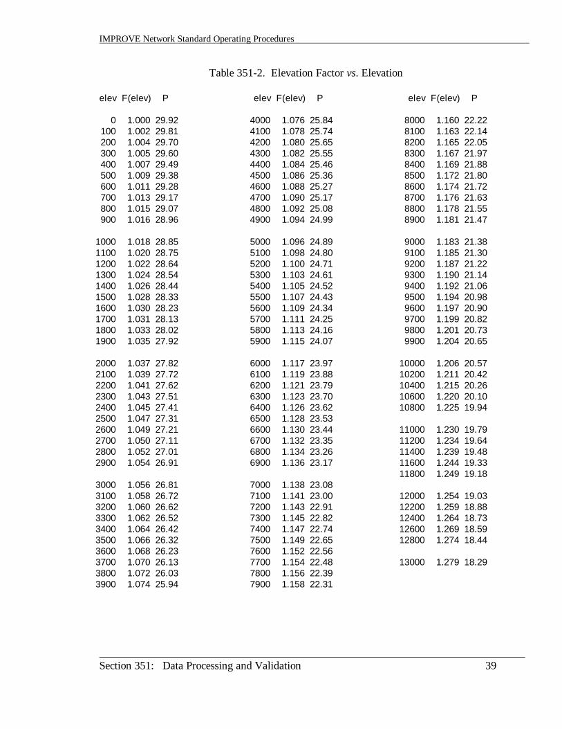
The values of nominal P and F(elev) as a function of elevation and for each site are given inTables 351-2 and 351-2.
IMPROVE Network Standard Operating Procedures
Section 351: Data Processing and Validation 39
Table 351-2. Elevation Factor vs. Elevation
elev F(elev) P
0 1.000 29.92100 1.002 29.81200 1.004 29.70300 1.005 29.60400 1.007 29.49500 1.009 29.38600 1.011 29.28700 1.013 29.17800 1.015 29.07900 1.016 28.96
1000 1.018 28.851100 1.020 28.751200 1.022 28.641300 1.024 28.541400 1.026 28.441500 1.028 28.331600 1.030 28.231700 1.031 28.131800 1.033 28.021900 1.035 27.92
2000 1.037 27.822100 1.039 27.722200 1.041 27.622300 1.043 27.512400 1.045 27.412500 1.047 27.312600 1.049 27.212700 1.050 27.112800 1.052 27.012900 1.054 26.91
3000 1.056 26.813100 1.058 26.723200 1.060 26.623300 1.062 26.523400 1.064 26.423500 1.066 26.323600 1.068 26.233700 1.070 26.133800 1.072 26.033900 1.074 25.94
elev F(elev) P
4000 1.076 25.844100 1.078 25.744200 1.080 25.654300 1.082 25.554400 1.084 25.464500 1.086 25.364600 1.088 25.274700 1.090 25.174800 1.092 25.084900 1.094 24.99
5000 1.096 24.895100 1.098 24.805200 1.100 24.715300 1.103 24.615400 1.105 24.525500 1.107 24.435600 1.109 24.345700 1.111 24.255800 1.113 24.165900 1.115 24.07
6000 1.117 23.976100 1.119 23.886200 1.121 23.796300 1.123 23.706400 1.126 23.626500 1.128 23.536600 1.130 23.446700 1.132 23.356800 1.134 23.266900 1.136 23.17
7000 1.138 23.087100 1.141 23.007200 1.143 22.917300 1.145 22.827400 1.147 22.747500 1.149 22.657600 1.152 22.567700 1.154 22.487800 1.156 22.397900 1.158 22.31
elev F(elev) P
8000 1.160 22.228100 1.163 22.148200 1.165 22.058300 1.167 21.978400 1.169 21.888500 1.172 21.808600 1.174 21.728700 1.176 21.638800 1.178 21.558900 1.181 21.47
9000 1.183 21.389100 1.185 21.309200 1.187 21.229300 1.190 21.149400 1.192 21.069500 1.194 20.989600 1.197 20.909700 1.199 20.829800 1.201 20.739900 1.204 20.65
10000 1.206 20.5710200 1.211 20.4210400 1.215 20.2610600 1.220 20.1010800 1.225 19.94
11000 1.230 19.7911200 1.234 19.6411400 1.239 19.4811600 1.244 19.3311800 1.249 19.18
12000 1.254 19.0312200 1.259 18.8812400 1.264 18.7312600 1.269 18.5912800 1.274 18.44
13000 1.279 18.29
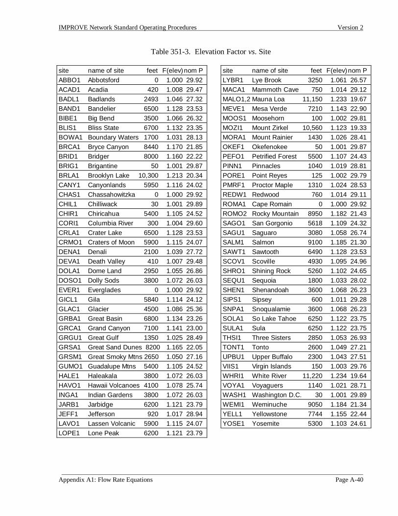
IMPROVE Network Standard Operating Procedures Version 2
Appendix A1: Flow Rate Equations Page A-40
Table 351-3. Elevation Factor vs. Site
site name of site feet F(elev)nom PABBO1 Abbotsford 0 1.000 29.92ACAD1 Acadia 420 1.008 29.47BADL1 Badlands 2493 1.046 27.32BAND1 Bandelier 6500 1.128 23.53BIBE1 Big Bend 3500 1.066 26.32BLIS1 Bliss State 6700 1.132 23.35BOWA1 Boundary Waters 1700 1.031 28.13BRCA1 Bryce Canyon 8440 1.170 21.85BRID1 Bridger 8000 1.160 22.22BRIG1 Brigantine 50 1.001 29.87BRLA1 Brooklyn Lake 10,300 1.213 20.34CANY1 Canyonlands 5950 1.116 24.02CHAS1 Chassahowitzka 0 1.000 29.92CHIL1 Chilliwack 30 1.001 29.89CHIR1 Chiricahua 5400 1.105 24.52CORI1 Columbia River 300 1.004 29.60CRLA1 Crater Lake 6500 1.128 23.53CRMO1 Craters of Moon 5900 1.115 24.07DENA1 Denali 2100 1.039 27.72DEVA1 Death Valley 410 1.007 29.48DOLA1 Dome Land 2950 1.055 26.86DOSO1 Dolly Sods 3800 1.072 26.03EVER1 Everglades 0 1.000 29.92GICL1 Gila 5840 1.114 24.12GLAC1 Glacier 4500 1.086 25.36GRBA1 Great Basin 6800 1.134 23.26GRCA1 Grand Canyon 7100 1.141 23.00GRGU1 Great Gulf 1350 1.025 28.49GRSA1 Great Sand Dunes 8200 1.165 22.05GRSM1 Great Smoky Mtns 2650 1.050 27.16GUMO1 Guadalupe Mtns 5400 1.105 24.52HALE1 Haleakala 3800 1.072 26.03HAVO1 Hawaii Volcanoes 4100 1.078 25.74INGA1 Indian Gardens 3800 1.072 26.03JARB1 Jarbidge 6200 1.121 23.79JEFF1 Jefferson 920 1.017 28.94LAVO1 Lassen Volcanic 5900 1.115 24.07LOPE1 Lone Peak 6200 1.121 23.79
site name of site feet F(elev)nom PLYBR1 Lye Brook 3250 1.061 26.57MACA1 Mammoth Cave 750 1.014 29.12MALO1,2 Mauna Loa 11,150 1.233 19.67MEVE1 Mesa Verde 7210 1.143 22.90MOOS1 Moosehorn 100 1.002 29.81MOZI1 Mount Zirkel 10,560 1.123 19.33MORA1 Mount Rainier 1430 1.026 28.41OKEF1 Okefenokee 50 1.001 29.87PEFO1 Petrified Forest 5500 1.107 24.43PINN1 Pinnacles 1040 1.019 28.81PORE1 Point Reyes 125 1.002 29.79PMRF1 Proctor Maple 1310 1.024 28.53REDW1 Redwood 760 1.014 29.11ROMA1 Cape Romain 0 1.000 29.92ROMO2 Rocky Mountain 8950 1.182 21.43SAGO1 San Gorgonio 5618 1.109 24.32SAGU1 Saguaro 3080 1.058 26.74SALM1 Salmon 9100 1.185 21.30SAWT1 Sawtooth 6490 1.128 23.53SCOV1 Scoville 4930 1.095 24.96SHRO1 Shining Rock 5260 1.102 24.65SEQU1 Sequoia 1800 1.033 28.02SHEN1 Shenandoah 3600 1.068 26.23SIPS1 Sipsey 600 1.011 29.28SNPA1 Snoqualamie 3600 1.068 26.23SOLA1 So Lake Tahoe 6250 1.122 23.75SULA1 Sula 6250 1.122 23.75THSI1 Three Sisters 2850 1.053 26.93TONT1 Tonto 2600 1.049 27.21UPBU1 Upper Buffalo 2300 1.043 27.51VIIS1 Virgin Islands 150 1.003 29.76WHRI1 White River 11,220 1.234 19.64VOYA1 Voyaguers 1140 1.021 28.71WASH1 Washington D.C. 30 1.001 29.89WEMI1 Weminuche 9050 1.184 21.34YELL1 Yellowstone 7744 1.155 22.44YOSE1 Yosemite 5300 1.103 24.61

IMPROVE Network Standard Operating Procedures Version 2
Appendix A1: Flow Rate Equations Page A-41
4.5.1.5 Calibration of Audit Devices
The reference flow rate is provided by a spirometer located in the sampler laboratory at UCD.The spirometer measurements are verified by a dry gas meter monitoring the exhaust to thecalibration pump. Taking the logs of Equation 351-7A, the flow rate equation for the auditdevice is
( ) ( )log log.
*logQ aP
Tb Mo o o= +
+
+
29 92 273293
. ...................... (351-11)
The log of the meter reading, Mo, is regressed against the log of the flow rate for a set of fourflow rates covering the normal range of the device. The constants relative to the nominal sealevel pressure (29.92) and 20°C are calculated using
aP
Tc = −
+
intercept log
.29 92 273293
b slopeo = . .................... (351-12)
4.5.1.6 Nominal Flow Rate Equation
In order to have a mean annual flow rate of 22.8 L/min at 15°C, the critical orifices areadjusted to provide a flow rate of 23 L/min at 20°C with a typical filter in the cassette. Forthe Wedding PM10 inlet the nominal flow rate is set at 19.1 L/min at 20°C, while for theSierra-Anderson PM10 inlet is set at 17.8 L/min. Using Equation 351-7b, the audit deviceflow rate at the site and 20°C is given by
Q M F elevoa
ob= =10 0 0 ( ) 23.0 L / min ................................. (351-13)
The desired reading on the audit device is
MF elevo a
b
=
23( )
/110 0
01
. ............................................ (351-14)
4.5.1.7 Flow Rate Equation for the System Vacuum Gauge
The measurement by the vacuum gauge is based on the equation for the critical orifice,Equation 351-2):
Q = Qo * 1 −
∆PP
*f(T) . ...............................................
We can redefine the Qo constant to include the elevation factor:
Q = Q3 * 1 −
∆PP
*f(T) F(elev) , ...................................... (351-15)

IMPROVE Network Standard Operating Procedures Version 2
Appendix A1: Flow Rate Equations Page A-42
where Q3 is another constant. We can write this in terms of parameters c and d as
Q = c + d*G *f(T) F(elev).............................................. (351-16)
The parameter d is negative. The parameters will be independent of temperature, but notindependent of pressure. That is, they would change if the sampler were moved to a newlocation. The form of this equation was chosen to keep it parallel to that of the system orificemeter.
4.5.1.8 Calibration of the System Orifice Meter and Vacuum Gauge
A four point calibration is made of the system orifice meter and the vacuum gauge at the siteusing an audit device to determine the flow rate at the inlet. The equations for the flow ratefrom the audit device (Q0), the system orifice meter (Om), and the vacuum gauge (Qg), allrelative to sea level and 20°C are:
Q Moa
ob= 10 0 0 ................................................... (351-17)
Q Mma b= 10 ..................................................... (351-18)
Q c d Gg = + * ...................................................... (351-19)
For each of the four points, Q0 is calculated using Equation 351-17. For the system orificemeter, the log of Q0 is regressed against the log of M: a is the intercept and b is the slope.For the vacuum gauge Q0 is linearly regressed with G: c is the intercept and d is the slope.
In the one point mail audit, M0, M, and G are recorded for both filters in each module andused to calculate the three flow rates relative to sea level and 20°C.

IMPROVE Network Standard Operating Procedures Version 2
Appendix A2: Concentration Equations Page A-43
4.5.2 Determination of Concentration, Artifacts and Precision
The following section is a discussion of the equations used to determine aerosolconcentration, both the sum and its parts, the artifacts produced by the analysis and analyticalprecision provided bye the analysis technique. They are broken into the following sections:
Artifact (4.5.2.1);Verification by Distributions (4.5.2.2);Definitions of Variables (4.5.2.3);Concentration (4.5.2.4);Volume (4.5.2.5);Analytical Precision (4.5.2.6);Gravimetric Mass (4.5.2.7);PIXE, XRF, and PESA Analysis (4.5.2.8);Ion, Carbon, and SO2 Analysis (4.5.2.9);Optical Absorption (4.5.2.10)
4.5.2.1 Artifact
Artifact is defined as any increase or decrease of material on the filter that positively ornegatively biases the measurement of ambient concentration. The five major types of artifactare
• contamination of the filter medium;• contamination acquired by contact with the cassettes or in handling;• adsorption of gases during collection that are measured as particles;• volatilization during collection and in handling;• fall-off during handling after collection.
The first three are positive artifacts and the last two negative. The first contamination artifactis determined by analysis of laboratory blanks. The sum of the two contamination artifacts isdetermined by analysis of dynamic field blanks (DFB's). These are handled as normal filters,except that no air is drawn through. The adsorption artifact on quartz filters is determined byanalysis of secondary filters. The assumption is that the first filter collects all of the particlesand does not significantly remove the relevant gases. The adsorbed gas appears as hightemperature organic. Comparison between quartz secondary and blank filters indicates thatsome of the low temperature artifact acquired in handling is volatilized during collection.There appears to be some adsorption of SO2 on the nylon filter at some sites; for this reasonwe do not include the nylon sulfate concentrations in the public data base.

IMPROVE Network Standard Operating Procedures Version 2
Appendix A2: Concentration Equations Page A-44
We do not correct for the two negative artifact types, volatilization and fall-off. Themeasured low temperature organics may be much less than in the atmosphere because ofvolatilization of particles during the remainder of the sampling. We assume that anyvolatilization of nitrate and chlorine from nylon is not significant. The fine mass on the Teflonfilter will be underestimate the ambient mass concentrations in high nitrate areas because somenitrates collected on Teflon will volatilize.
4.5.2.2 Verification by Distributions
The blanks and secondary filters may not always provide reasonable values for the artifact. Inorder to verify an estimate from field blanks, we examine the distribution of values for ambientsamples in two ways. We first examine the minimum of the ambient values for a large set ofsamples. If we can reasonably assume that the ambient mass of a given variable isoccasionally much less than the artifact, then the minimum measured values of the ambientsamples should equal the artifact. To avoid statistical problems, we often examine the 1%level, rather than the actual minimum.
We also examine the intercepts of regression plots of the variable with concentrations ofrelated variables that have no problems with artifact subtraction.
4.5.2.3 Definitions of Variables
Variables calculated prior to sample measurement:B = artifact mass (ng/filter) = mean of the DFB's or secondary filtersσdfb = standard deviation of the DFB's or secondary filters used to determine Bσa = component of analytical precision that is a constant mass per filter.fa = component of analytical precision that is a constant fraction. fa
fv = fractional volume precision = fractional flow rate precision
Variables measured or calculated with each sample:A = mass measured on real sample (ng/filter)V = volume (m3)area = area of deposit on the filter (cm2) , determined from the mask sizefs = analytical precision associated with counting statistics, expressed as fractionc = concentration (ng/m3)σ(c) = precision of c (ng/m3)
4.5.2.4 Concentration
The mass of material on the filter is equal to the difference between the mass measured on thesample and the artifact determined from field blanks and secondary filters. The concentrationequals this number divided by the volume:
c = A - B
V ...................................................... (351-20)
IMPROVE Network Standard Operating Procedures Version 2
Appendix A2: Concentration Equations Page A-45
4.5.2.5 Volume
The volume is the product of the average flow rate and the sample duration. The sampleduration is determined using an elapsed time indicator based on line frequency. The actualtime of start and stop is determined by the clock controller using an internal quartz crystal.The fractional precision of the volume is the quadratic sum of the fractional precisions of flowrate and duration. Since the fractional precision of the duration is always much smaller thanthat of the flow rate, it can be safely neglected.
The flow rate is measured before and after the collection each using two independentmethods. The first method measures the pressure drop across the cyclone using a magnehelicand employs the standard measuring orifice equation. The second method measures thepressure drop across the filter and employs the equation for flow through a critical orifice.The equations for flow rate are given earlier in this document. The average flow rate isnormally an average of the magnehelic flow rates before and after collection. If themagnehelic readings are determined to be in error, then the gauge measurements are used.
The precision in the average flow rate has two components: the precision in the measuredvalues and the uncertainty in assuming that the average flow rate during collection equals theaverage of the flow rates measured before and after collection. The precision in a measuredvalue is less than 3%, as estimated from internal and third-party audits. Most audits indicatethat the total precision/accuracy of the difference between an audit and an IMPROVEmeasurement is approximately 3%. Since the precisions of most audit devices are 2-3%, theIMPROVE flow rate precision must be less than 3%.
The second component of the precision is present because all flow control devices introduceuncertainty. A critical orifice device is extremely reliable, avoiding large errors at extremetemperatures, but does allow small variations in flow rate with temperature. A difference inaverage temperature during the sampling period from the average temperatures before andafter collection will produce an incorrect value of flow rate. Suppose both change days(Tuesdays) are colder than a sample day (e.g. Saturday). If the 24-hour mean temperaturewere 10°C higher than the average of the two measured temperatures, than the error inaverage flow rate would be 2%. We allow such unusual conditions by using a conservativevalue for the precision in the volume of 3%. This value has been used in all calculations forthe IMPROVE sampler. Calculating site-specific or seasonal precisions would complicate thecalculations without significantly changing the overall precision estimate of the concentrations.
4.5.2.6 Analytical Precision
1. Counting Statistics
There will be uncertainty associated with counting statistics whenever the measurement isbased on the number of counts from a detector. Gravimetric and IPM analyses do notinvolve counting statistics. We are not provided the information on counting statistics for

IMPROVE Network Standard Operating Procedures Version 2
Appendix A2: Concentration Equations Page A-46
ion chromatography and carbon combustion. Counting statistics are generally negligiblefor ion chromatography. They may not be negligible for carbon combustion, but weassume that any statistical precision is accounted for in the constant portion of the non-statistical precision. However, the statistical precision must be included for PIXE, XRF,and PESA because of a relatively large background in the spectra and the absence ofdirect artifact subtraction. This will be discussed in more detailed in the section on PIXE.
2. Non-statistical Analytical Precision
For simplicity we will assume that the non-statistical component of the analytical precisionmay consist of a constant mass/filter (σa and a constant fraction (fa). Theory indicates thatsome methods, such as gravimetric analysis, have only a σa component. The constantfraction form (fa) is appropriate for uncertainty associated with normalization andcalibration. In x-ray systems, fa represents the uncertainty in normalizing each analysis toan incident beam intensity. In ion chromatography fa includes the precision in preparing analiquot. X-ray methods have only a fa component. For ion chromatography and carboncombustion we will assume both components are present.
3. The total analytical precision in the measured value A (mass/filter) is given by
[σ(A)]2 = σa2 + (A*fa)2 + (A*fs)2 ....................................... (351-21)
4. Calculation of Factors for Analytical Precision
We determine the two non-statistical components, σa and fa, from replicate analyses. Wewill assume that for each replicate pair the difference is produced by the three factors ofEquation 351-21.
For the elemental analyses, where σa is zero, the difference is produced by fa and fs. The fa
factor is determined from elements in which the statistical factor is negligible. For PIXEwe chose sulfur for sites where there is always abundant sulfur and for XRF we chooseiron. In both cases, fs is zero. Historically, fa has historically equaled 4% for S by PIXEand for Fe by XRF. Rather than allow this value to vary each season based on theindividual analysis run, we have used 4% throughout.
For ion chromatography and carbon combustion we assume each measurement is given byEquation 351-21 with fs=0. For each pair of replicate analyses we calculate M = mean andP = difference / 2 . The relationship between P and M is
Pf
f Maa a
22
2 2 212
−
= +σ * . ......................................... (351-22)
The term in brackets is always close enough to 1.00 to justify setting it equal to 1. To tocalculate σa and fa , P is plotted against M and the best values are obtained by examining

IMPROVE Network Standard Operating Procedures Version 2
Appendix A2: Concentration Equations Page A-47
the regions of low and high M. At low M, σa = P. At high M, fa equals the slope. Thisapproach has the added feature of verifying the validity of separating the analyticalprecision into the two factors.
4.5.2.7 Gravimetric Mass
In the case of gravimetric analysis, the analytical precision is independent of the magnitude ofthe measured value, so that both fa and fs are zero. Thus, the analytical precision in ng/filter,σa, is the same for all samples, including DFB's.
The standard deviation of the DFB's may be expressed as the sum of the precision in theartifact and the precision in the analysis.
σdfb2 = [σ(B)]2 + σa
2 . ................................................. (351-23)
The precision in the artifact-corrected mass is the sum of the precision of the measurement,σa, and the precision in B and is given by
[σ(A-B)]2 = σa2 + [σ(B)]2 ............................................ (351-24)
Thus, the precision in the difference (A-B) is equal to the standard deviation in the DFB's
σ(A-B) = σdfb ....................................................... (351-25)
The precision in the concentration may be written as
[σ(c)]2 = σdfb
V
2
+ (fv*c)2............................................. (351-26)
We define the minimum detectable limit as the concentration that is equal to 2σ. The exactexpression is given by
mdl = 21
1 4 2
σdfb
V
−
f v
. ........................................... (351-27)
The right- term equals 1.002 for fv=0.03. The difference from 1.00 is negligible compared tothe uncertainties in σdfb and V. We will use the simpler expression
mdl = 2σdfb
V ....................................................... (351-28)
4.5.2.8 PIXE, XRF, and PESA Analysis
In PIXE, XRF, and PESA, the spectral background for a sample is estimated using a spectrumof a blank Teflon filter. This procedure removes any contaminants, if present. These spectraof blank filters indicate that any elemental artifact is extremely small. Therefore the

IMPROVE Network Standard Operating Procedures Version 2
Appendix A2: Concentration Equations Page A-48
concentration is calculated using B=0. We use a variation of Equation 351-20, because PIXE,XRF, and PESA determine mass per unit area rather than mass per filter. This areal density inng/cm2 is proportional to the number of counts in the peak, with the proportionality factordepending on the element, the number of protons, and the detector live time. The spectralanalysis program is provided the ratio of deposit area divided by sample volume. Theconcentration is calculated using
c = k * N * areaV
, ................................................... (351-29)
where area is the area of deposit on the filter, N is the number of counts in the peak, and k is aconstant depending on the element, the number of protons, and the detector live time.
None of the three methods have a constant component to the precision, so that σa=0. Allhave constant fractional components, (fa), associated with normalizing to the incident beam.The value of fa is measured every analytical session using replicate analyses for elements withnegligible statistical precision. It has never varied significantly from 4%. We have maintaineda constant value of fa=0.04 in the data processing since 1988.
Measurements by all three methods have a statistical component to the precision, (fs), basedon the number of counts in the peak and in the background under the peak. Assuming aPoisson distribution, N counts in the peak, and Nb background counts under the peak, thefractional statistical precision is given by
fs2 =
11 2
NNN
b+
................................................... (351-30)
The precision of the concentration is given by
[σ(c)]2 = c2 * (fs2 + fa
2 + fv2 ) . .......................................... (351-31)
The precision is calculated separately for each variable at the time of spectral analysis using fa
= 0.04 and fv = 0.03. The quadratic sum of these two is 0.05. At small concentrations thestatistical term is dominant, while at large concentrations the precision approaches 5%. Forsulfur, the average precision for all sites and seasons is slightly larger than 5%.
The minimum detectable limit for each PIXE variable is calculated from the background in thespectrum at the location of the peak and the relationship between counts and concentration forthat peak. The mdl is defined as the concentration at which the number of valid counts equals3.3 times the square root of the background counts under the peak. The mdl defines theupper limit that a variable can be reliably observed in the spectrum, although it is possible tofind peaks with concentrations slightly below the mdl. At the mdl, the analytical precision isapproximately 50% of the mdl. The mdl is calculated separately for each variable at the timeof spectral analysis.

IMPROVE Network Standard Operating Procedures Version 2
Appendix A2: Concentration Equations Page A-49
4.5.2.9 Ion, Carbon and SO2 Analysis
The equations for these three methods are the same, except for SO2, where the concentrationsare multiplied by 2/3 to convert from SO4 to SO2. The methods are characterized bysignificant artifact and unknown statistical precision.
The standard deviation of the DFB's or secondary filters includes the precision in the artifactand the analytical precision. (As in the case of gravimetric analysis, we do not equate theprecision in the artifact with the standard deviation of the DFB's.) The standard deviation is aquadratic sum of the precision of the artifact B, the constant analytical precision, and thefractional analytical precision:
σdfb2 = [σ(B)]2 + σa
2 + [fa*B]2........................................... (351-32)
The precision of the mass/filter of the sample is
[σ(A)]2 = σa2 + [fa*A]2. ............................................... (351-33)
The precision of the difference (A-B) is obtained by quadratically adding the precisions of Aand B,
[σ(A-B)]2 = [σ(A)]2 + [σ(B)]2........................................... (351-34)
The precision of the concentration is therefore given by
[ ] [ ] [ ]σσ σ
(c)2
22
2 22=
−
+ =
+
+( )
*( )
* *A BV
f cB
Vf
AV
f cv a v . ............ (351-35)
This can be written in terms of the constants as
[ ] ( )σσ
(c)2
22 2 2 22
=
+
+ +dfb
a a vVB
Vf c f f c* * * . .......................... (351-36)
Note that the constant analytical precision, σa, does not appear in Equation 351-36. Thisportion of the precision is included indirectly in σdfb.
For small c, the first term in Equation 351-36 is dominant, while for large c, the third term isdominant. The second term is never dominant; the maximum contribution for mostparameters is less than 10%.
The minimum detectable limit is defined as the concentration that is twice the precision.Solving Equation 351-36 for the concentration gives

IMPROVE Network Standard Operating Procedures Version 2
Appendix A2: Concentration Equations Page A-50
mdl = 21
1σdfb
V
− − +−
h g gh
, ...................................... (351-37)
where g = 2Bσdfb
fa
2 h = 4(fa2 + fv
2 ) .
Retaining the second order terms would increase the estimate of the mdl less than 2% for ionchromatography and organic carbon. The simplified form that drops second order terms isused in the data processing:
mdl = 2 σdfb
V ....................................................... (351-38)
4.5.2.10 Optical Absorption
The calculation of the coefficient of absorption does not follow Equation 351-20. Themodified Laser Integrating Plate Method (LIPM) system has a 2" sphere to measure reflectedlight and an integrating to measure a fraction of the transmitted light. The exposed side of thefilter is always placed away from the source, so that the light first passes through the Teflon.The system is calibrated by reference to our 6" research integrating sphere. The LIPM spheredetector is adjusted to give the same value of R for a reference filter as the research sphere inthe reflectance mode. The LIPM plate detector is adjusted to give the same value of T as theresearch sphere in the transmittance mode. In the data processing system, the absorptionmeasured on the filter is labeled LRNC for 'laser not corrected'. (The ambient coefficient isconsidered a composite variable and is labeled BABS.) For area in cm2 and volume in m3, theequation for the uncorrected coefficient of absorption in 10-8 m-1 is
LRNCR
T=
−
areaV
1010004 ln . .................................... (351-39)
No measurement of the clean filter is needed because Teflon does not absorb light. Becauseof layering effects inherent in collecting particles on a filter, the absorption measured on thefilter (LRNC) is less than the ambient absorption (BABS). The parameter BABS is discussedin section 4.5.3. The uncertainty in LRNC is determined by replicate measurements ofambient filters.
[ ] ( )σ( ) *LRNCareaV
f LRNCv2
22
225.=
+* ............................. (351-40)
Note that because of the relative large uncertainty in the mass correction, this uncertainty inLRNC is generally much less than the final uncertainty in BABS.
The minimum detectable limit is defined as twice the precision in the measurement for asample with low absorption. The approximate expression for the mdl in 10-8 m-1 is then

IMPROVE Network Standard Operating Procedures Version 2
Appendix A2: Concentration Equations Page A-51
mdl = areaV
* 450.................................................... (351-41)
For a typical filter with a collection area of 2.2 cm2, the mdl is approximately 30 10-8 m-1 or0.3 (Mm)-1.

Appendix A3: Equations of Composite Variables Page A-52
4.5.3 Equations of Composite Variables
The following composite variables are combinations of the measured concentrations of particlescollected on the fine filters. These are used in the level II validation procedures and in theseasonal summaries.
The precision of each concentration is determined along with the value of the concentration andthe minimum detectable limit (mdl) of each concentration. In our calculations of the precision ofthe composite variables, we will assume that the component concentrations are independent andthe multiplicative factors have no uncertainty. The independence assumption is not strictly validfor many composites because of common factors, such as volume. However, the effect on theoverall precision is too small to warrant the more complicated calculations. The followingsections are divided by composite. They are as follow:
Sulfate by PIXE (S3) and Ammonium Sulfate (NHSO) (4.5.3.1);Ammonium Nitrate (NHNO) (4.5.3.2);Soil (4.5.3.3);Non-soil Potassium (KNON) (4.5.3.4);Light-Absorbing Carbon (LAC) (4.5.3.5);Ambient Coefficient of Absorption (BABS) (4.5.3.6);Organics by Carbon (OMC) (4.5.3.7);Organics by Hydrogen (OMH) (4.5.3.8);Reconstructed Mass from the Teflon Filter (RCMA) (4.5.3.9);Reconstructed Mass using Carbon Measurements (RCMC) (4.5.3.10)
4.5.3.1 Sulfate by PIXE (S3) and Ammonium Sulfate (NHSO)
Sulfur is predominantly present as sulfate. To compare the sulfur by PIXE and the sulfate byion chromatography, the PIXE concentration is multiplied by 3.0. This composite is labeledS3.
The sulfate is generally present as ammonium sulfate, (NH3)2SO4, although it can be presentas ammonium bisulfate, (NH3)HSO4, sulfuric acid, H2SO4, and, in marine areas, as sodiumsulfate, NaSO4. In many of these cases, the particle will include associated water, but w omitthis from the calculation. In order to simplify the calculation we will assume all the sulfur ispresent as ammonium sulfate. The concentration and precision is given by:
NHSO = 4.125 * S................................................... (351-42)σ(NHSO) = 4.125 * σ(S).............................................. (351-43)
(Strictly, the factor should be 4.121, but 4.125 is the traditional value.) If S is below the mdl,both S and σ(S) are set equal to mdl/2. For ammonium bisulfate, sulfuric acid, and sodiumsulfate the factors are 3.59, 3.06, and 4.43, respectively. In the first two cases, the actual drymass associated with sulfate will be less than NHSO, and in the third case, more.

Appendix A3: Equations of Composite Variables Page A-53
4.5.3.2 Ammonium Nitrate (NHNO)
This composite is the total dry concentration associated with nitrate, assuming 100%neutralization by ammonium. For all sites, we define the ammonium nitrate concentration andprecision by:
NHNO = 1.29 * NO3- ................................................ (351-44)σ(NHNO) = 1.29 * σ(NO3-) ........................................... (351-45)

Appendix A3: Equations of Composite Variables Page A-54
4.5.3.3 SOIL
The soil component consists of the sum of the predominantly soil elements measured by x-rayanalysis, plus oxygen for the normal oxides (Al2O3, SiO2, CaO, K2O, FeO, Fe2O3, TiO2), plusa factor for other compounds, such as MgO, Na2O, water, and CO2. The followingassumptions are made:• We will assume that the Fe is split equally between FeO (oxide factor of 1.29) and Fe2O3
(oxide factor of 1.43), giving an overall Fe oxide factor of 1.36.• Fine K has a non-soil component from smoke. Based on the K/Fe ratio for average
sediment (Handbook of Chemistry and Physics) of 0.6, we use 0.6*Fe as a surrogate forsoil K. With the oxide factor of K, this is increases the factor for Fe from 1.36 to 2.08.
• Because aluminum has not always been detected with as high a frequency as the othermajor soil elements, we have eliminated Al from the soil parameter. Fortunately, thecorrelation between Al and Si is excellent for all sites, with a constant ratio of Al/Si of0.45. With the oxide factors for Al2O3 and SiO2 the multiplicative factor for Si increasesfrom 2.14 to 2.99 . The only exception is Virgin Islands, where the Al/Si ratio is 0.60; thesoil parameter is then low by 6%.
• The oxide forms of the soil elements account for 86% of average sediment; in order toobtain the total mass associated with soil, the final factors are divided by 0.86 (handbookof Chemistry and Physics. The final equations for fine soil concentrations and precisionare:
SOIL = 2.20*Al + 3.48*Si + 1.63*Ca + 2.42*Fe + 1.94*Ti.................... (351-46)[σ(SOIL)]2 = [3.48*σ(Si)]2 + [1.63*σ(Ca)]2 + ... .......................... (351-47)
The soil variable is calculated for all valid PIXE analyses. If an element is below the mdl, theconcentration and precision are both assumed to be equal to mdl/2. The soil variable is alwayspositive.
4.5.3.4 Non-soil Potassium (KNON)
Non-soil K is the measured fine K minus the soil K estimated from Fe. Non-soil K is aqualitative tracer of smoke, but may not be a quantitative measure of the mass of smokeaerosol. The problem is that the ratio of K / smoke mass may change as the aerosol ages.Particulate smoke K is probably produced by transformation of volatilized K, and appears tobe on smaller particles than most smoke mass. When close to the source, the particulate Kmay not have time to form. For long transport, most other smoke mass may settle out morethan K mass. The concentration and precision of KNON are:
KNON = ( K - 0.6*Fe ) ............................................... (351-48)σ2(KNON) = σ2(K) + [0.6*σ(Fe)]2....................................... (351-49)
The soil factor of 0.6 may vary slightly with site; this will produce a small positive or negativeoffset for baseline values, when no smoke is present. Therefore, negative values are retained.
Appendix A3: Equations of Composite Variables Page A-55
KNON is defined for all valid PIXE analyses. If a concentration is less than the mdl, theconcentration and precision are assumed to be equal to mdl/2.
4.5.3.5 Light-Absorbing Carbon (LAC)
The concentration of carbon on quartz is determined in seven temperature ranges, plus acorrection fraction for pyrolized organic. The light-absorbing component is assumes to be allcarbon evolved at 550°C and above after the laser indicates that reflectance has returned tothe initial value. The equation for concentration is:
LAC = E1 + E2 + E3 - OP ............................................ (351-50)
LAC may be negative. The uncertainty of LAC is not the quadratic sum of the components.Based on replicate measurements, the best estimate of uncertainty is:
( ) ( )σ LAC LAC= +( ) . *34 0 0672 2 ng/m3 ................................ (351-51)
4.5.3.6 Ambient Coefficient of Absorption (BABS)
BABS has an unusual position in the data base. The uncorrected coefficient of absorption,LRNC, is stored in the internal data base, but is not provided for external users. The externalusers are only provided with the corrected ( or ambient) coefficient.
The first and smallest correction is associated with the integrating plate method. In theintegrating plate method any scattering with angles large enough to miss the plate causes anincrease in apparent absorption. In order to quantify the effect of the large angle scattering, aseries of comparisons were made between the integrating plate system and an integratingsphere system. The integrating sphere system, is somewhat more difficult to use routinely, buteliminates the scattering component. Comparison of the results indicates that approximately3% of the apparent absorption by LIPM is associated with scattering. The measuredcoefficient is therefore multiplied by 0.97.
Several tests involving simultaneous measurements of the same atmosphere but with differingmass per unit area (areal density) have shown that it is necessary to correct the valuesmeasured on a filter to obtain the proper atmospheric absorption. This is true for bothintegrating plate and integrating sphere. The correction is small for very lightly loadedsamples, but we are constrained to design a sampler primarily for other particle measurements.The hypothesis is that the absorption of particles on a filter is less than the ambient absorptionof particles because other particles on the filter can shield a given absorbing particle. A formwas chosen that included two exponents of the areal density of particles measured bygravimetric analysis in µg/cm2. Note that the effect is observed even if the layeringmechanism is not correct. The equation used is
R = 0.36 expt
22+ 0.64 exp
t415
−
−
ρ ρ .................................. (351-52)
Appendix A3: Equations of Composite Variables Page A-56
where the constants were determined by fitting data from independent studies at Davis andLos Angeles.
The equation for the ambient coefficient of absorption in 10-8 m-1 is derived from theuncorrected coefficient using:
BABS = LRNC * 0.97
R . .............................................. (351-53)
The uncertainty in R is estimated to be 10% of (1-R), based on the precision of the fit for thetest data. The equation for the precision of the corrected coefficient of absorption is:
σ(BABS) = ( )σ LRNC *0 97
01012 2.
. * *R
RR
b
+
−
........................ (351-54)
The minimum detectable limit is defined as twice the precision in the measurement for asample with low absorption. Although this will vary with the intensity for a clean filter, it ismore convenient to use a single intensity of 390 units for a typical clean filter. The expressionfor the mdl is then approximately
mdl(BABS) = mdl(LRNC) * 0.97
R....................................... (351-55)
The concentration of absorbing particles can also be estimated from the coefficient ofabsorption using the absorption efficient ε in m2/g. For high temperature elemental carbon,such as diesel emissions, the value of ε is typically 10 m2/g. Thus the concentration ofabsorbing carbon in ng/m3 is numerically equal to BABS in 10-8 m-1.
However, the comparison of BABS and the concentration light absorbing carbon, LAC,indicates that the BABS method yields a concentration that is approximately twice that ofLAC. The two variables are moderately correlated (r=0.74 for western sites). There are threepossible explanations:
• The UCD integrating plate and integrating sphere methods both give values of babsthat are high by a factor of 2.
• The absorption efficient of 10 m2/g is not appropriate for the low temperatureelemental carbon measured at remote sites.
• Some of the organic carbon absorbs light. There is a better relationship if we assumethat all carbon evolved at 550°C absorbs light with an absorption efficient of 10 m2/g.
Appendix A3: Equations of Composite Variables Page A-57
4.5.3.7 Organics by Carbon (OMC)
The concentration of carbon on quartz is determined in seven temperature ranges, plus acorrection fraction for pyrolized organic. The organic component is assumes to be all carbonevolved at 550°C and below in a pure helium environment, plus the pyrolized organic fraction.The equation for concentration is:
OMC = 1.4 (O1 + O2 + O3 + O4 + OP) ................................. (351-56)
OMC may be negative. The uncertainty of OMC is not the quadratic sum of the components.Based on replicate measurements, the best estimate of uncertainty is:
( ) ( )σ OMC OMC= +( ) . *168 0 052 2 ng/m3 ............................... (351-57)
4.5.3.8 Organics by Hydrogen (OMH)
The organic mass can also be calculated from the concentrations of H and S measured on theTeflon filter. The assumptions are:
• All sulfur is present as fully neutralized ammonium sulfate. This is valid at all sitesexcept those in the East with high sulfur, and at marine sites with significant marinesulfate.
• All nitrates and water volatilize during exposure to vacuum, so the PESA hydrogencomes only from sulfates and organics. This assumption is valid at all except thosesites in California with such high nitrate concentrations that some hydrogen remains.
• The average organic particle contains 9% hydrogen. That is, we must multiply theorganic hydrogen by 11 to estimate total organic mass.
The equations for OMH concentration and precision are:
OMH = 11 ( H - 0.25 * S )............................................. (351-58)σ2(OMH) = (11)2 [σ2(H) + [0.25*σ(LAC)]2................................ (351-59)
If either H or S are invalid or not detected (below mdl), then OMH is not calculated. OMHmay be negative when the sulfate is large and not fully neutralized.
At sites where the above assumptions are reasonable, the resulting estimate is in goodagreement with organic mass by carbon, OMC, except for the multiplicative constant of 11.For all western sites excluding those with high ammonium nitrate and marine sulfur (SanGorgonio, Pinnacles, Point Reyes and Redwood) the correlation is good (r=0.89) and theslope is very close to 0.80. There are two possible explanations for the 80% ratio betweenOMC and OMH as defined above. One is that the volatile organic hydrogen component islost in vacuum. The second explanation is that the carbon analytical methods attributes someof the elemental carbon to the organic fraction. Either change shifts the ratio close to 1. Ateastern sites the OMH concentration is sometimes much less than OMC, and is occasionallynegative. For these samples some of the sulfate is present as sulfuric acid.

Appendix A3: Equations of Composite Variables Page A-58
4.5.3.9 Reconstructed Mass from the Teflon filter (RCMA)
The reconstructed mass is the sum of sulfate, soil, non-sulfate potassium, salt, elementalcarbon, and organic carbon. The only components not included are water and nitrate. Asignificant fraction (>50%) of the nitrate particles volatilize from the Teflon filter duringcollection and is not measured by gravimetric analysis. The nitrate measured in theIMPROVE system is collected on nylon filters and do not volatilize during collection.Therefore, we have chosen to exclude the measured nitrate from the reconstructed mass.Nitrate collected on nylon filters should not be included in the reconstructed mass whencomparing it to the gravimetric mass on the Teflon filter. However, when estimating theactual ambient mass, one should add 1.29*NO3- to the reconstructed mass.
We will use two estimates of reconstructed mass: RCMA, based only on the Teflon filter andusing BABS/2 for elemental carbon and OMH for organic mass; and RCMC, based partly onthe carbon measurements from the quartz filter and partly on measurements from the Teflonfilter. The equations for RCMA concentration and precision are:
RCMA = 4.125*S + SOIL + 1.4*KNON + 2.5*Na+ BABS/2 + OMH............ (351-60)σ2(RCMA) = [4.125*σ(S)]2 + [σ(SOIL)]2 + [1.4*σ(KNON)]2 + ................. (351-61)
For RCMA to be calculated, PIXE, PESA, and LIPM must all have valid analyses. The 1.4factor with KNON ensures consistency with the soil estimate; it exactly compensates for theremoval of non-soil K from soil. Thus potassium is included in the sum as K2O, whether assoil or as smoke. The salt (NaCl) concentration is estimated solely from Na, because some ofthe chlorine is volatilized from the Teflon filter during collection. If S, Na, or babs are belowthe mdl, mdl/2 is used as both concentration and precision. KNON is used as calculated, evenif negative. If OMH is negative, a value of zero is used in the sum. RCMA will always bepositive.
4.5.3.10 Reconstructed Mass using Carbon Measurements (RCMC)
An alternative estimate is based on organics and elemental carbon from the quartz filter. As inRCMA, the sum does not include water and nitrates. The equation for RCMC is:
RCMC = 4.125*S + SOIL + 1.4*KNON + 2.5*Na+ LAC+ OMC............... (351-62)
For RCMC to be calculated, PIXE and carbon combustion must both have valid analyses. IfLAC or OMC is negative, a value of zero is used. RCMC will always be positive. .
In general, RCMA is preferred during periods of low organic concentrations, such as winter inwestern United States. RCMC is preferred at sites where the neutralization of sulfate may beless than 100%, at sites with high nitrate, and at marine sites.

SOP 351: Data Processing and Validation 59
4.5.4 Statistical calculation
The following sections deal with statistical equations used through out the qualityassurance process. They are divided into the following sections:
Slope and Intercept for Perpendicular Fit (4.5.4.1);Pair-wise Precision (4.5.4.2);Pair-wise Chi-Square (4.5.4.3)
4.5.4.1 Slope and Intercept for Perpendicular Fit
The validation procedures include examination of correlation plots between twovariables. Because both variables has associated uncertainty, it is necessary toconstruct the regression line that minimizes the perpendicular deviations of the pointsfrom the straight line. To do this it is first necessary to calculate the various means:
< > ==∑x
nx i
i
n1
1 < > =
=∑y
ny i
i
n1
1..........................................
( )< >==∑x
nx i
i
n2 2
1
1 ( )< >=
=∑y
ny i
i
n2 2
1
1 < > =
=∑xy
nx yi i
i
n1
1.................. (351-63)
The variances are calculated from the means:( )S x xx =< > − < >2 2 ( )S y yy =< > − < >2 2
S xy x yxy =< > − < > < > ......... (351-64)
The correlation coefficient is
( )r
S
S Sxy
x y
2
2
= .......................................................... (351-65)
The expression for the slope involves the difference between the x and y variances:
SS S
dy x=
−2
......................................................... (351-66)
We will the equation for the line to be y = a+bx. The slope b is given by:
( ) ( )slope b
S S S
Sd d xy
xy= =
+ +2 2
.......................................... (351-67)
The intercept a is given by:intercept = =< > − < >a y b x ............................................. (351-68)
To calculate the precisions in a and b, we first calculate the parameters f and g:

SOP 351: Data Processing and Validation 60
fS b S
Sy x
xy=
+ 2 g f b= − 2 .............................................. (351-69)
The precision of the slope is:
σbfg
n2
2=
−........................................................... (351-70)
The precision of the intercept is:
σ σa bxyx
g S
n2 2 2
2= < > +
−.............................................. (351-71)
4.5.4.2 Pair-wise Precision
The pair-wise relative precision is included on the plots for replicate analyses or for thesame parameter by different analytical methods. For replicate analyses with negligiblestatistical or constant precision, this parameter gives the relative analytical precisiondiscussed in section 4.5.2.
For multiple measurements of a single quantity, z, the absolute precision is thestandard deviation and the relative precision is the standard deviation divided by themean. The "unbiased estimate" of the standard deviation is defined as
( ) ( )[ ]stdevn
nz z2 2 2
1=
−< > − < > ......................................... (351-72)
Suppose there are only two measurements of each quantity, x and y. The standarddeviation for this pair is given by Equation 351-72 with n=2:
( ) ( )stdevx y x y
x y22 2 2
222 2
12
= + − +
= − ................................ (351-73)
If D is the absolute difference x y− and M is the mean, the standard deviation andrelative precision are:
stdev D= 12
PDM
= 12
.............................................. (351-74)
Suppose there are n such pairs. The overall precision is the root-mean-square of theindividual precisions. The absolute precision, Pabs is the sum of the individualstandard deviations, while the relative precision, P, is the sum of the individual relativeprecisions:
Pn
Dabs ii
n2 2
1
12
==∑ P
nDM
i
ii
n2
1
21
2=
=∑ ..................................... (351-75)
These can also be written in terms of the x's and y's as:

SOP 351: Data Processing and Validation 61
( )Pn
x yabs i ii
n2 2
1
12
= −=∑ P
nx yx y
i i
i ii
n2
1
22=
−+
=∑ .............................. (351-76)
4.5.4.3 Pair-wise Chi-Square
The pair-wise goodness-of-fit parameter, χ2, is also included on the plots for replicateanalyses or for the same parameter by different analytical methods. This parameter,compares the differences with the precision of the differences as determined for theprecision of x and y included in the data base. It is thus the best method ofdetermining whether the differences are within the predicted precision.
If σx and σy are the calculated precisions for x and y, the precision of the difference is:σ σ σd x y
2 2 2= + ......................................................... (351-77)
The goodness-of-fit parameter, χ2, is:
( )χ σ σ σ
2
2 2
2 2
1 1=
=
−+∑ ∑n
Dn
x y
d
i i
x y
........................................ (351-78)
Large values of χ2 indicate that there are probably sources of difference not included inthe estimate of precision.
4.6 Transfer of Data to Final Concentrations Database
The final data set is presented in several ways to the end users. The final database thatgets passed onto the masses takes the form of a simple ASCII file. Each ASCII file isdesignated with a site code and season code to identify the place and season of aerosoldata contained within. The following is a short sample of the database that is provided tothe end users:
********************************************************************************* Use of IMPROVE data requires acknowledgment both of its production by the ** Air Quality Group at the University of California at Davis and of its funding** by the National Park Service, US Department of Interior. ********************************************************************************* ACAD1 06/01/96 0000 24.00 23.6 MF 8386.30 291.50 294.30 NM ACAD1 06/01/96 0000 0.00 0.0 BABS 872.95 94.19 87.20 NM ACAD1 06/01/96 0000 0.00 0.0 MT 14264.30 467.30 375.40 NM ACAD1 06/01/96 0000 24.00 23.6 H 394.81 20.96 3.37 NM ACAD1 06/01/96 0000 24.00 23.6 NA 101.20 9.87 12.85 NM ACAD1 06/01/96 0000 24.00 23.6 MG 0.00 0.00 7.42 NM ACAD1 06/01/96 0000 24.00 23.6 AL 56.37 5.89 4.81 NM ACAD1 06/01/96 0000 24.00 23.6 SI 111.95 7.58 3.93 NM ACAD1 06/01/96 0000 24.00 23.6 P 0.00 0.00 3.77 NM ACAD1 06/01/96 0000 24.00 23.6 S 621.16 32.51 3.59 NM ACAD1 06/01/96 0000 24.00 23.6 CL 0.00 0.00 3.42 NM ACAD1 06/01/96 0000 24.00 23.6 K 56.63 3.69 2.16 NM ACAD1 06/01/96 0000 24.00 23.6 CA 35.42 2.79 1.69 NM ACAD1 06/01/96 0000 24.00 23.6 TI 7.18 1.36 1.53 NM
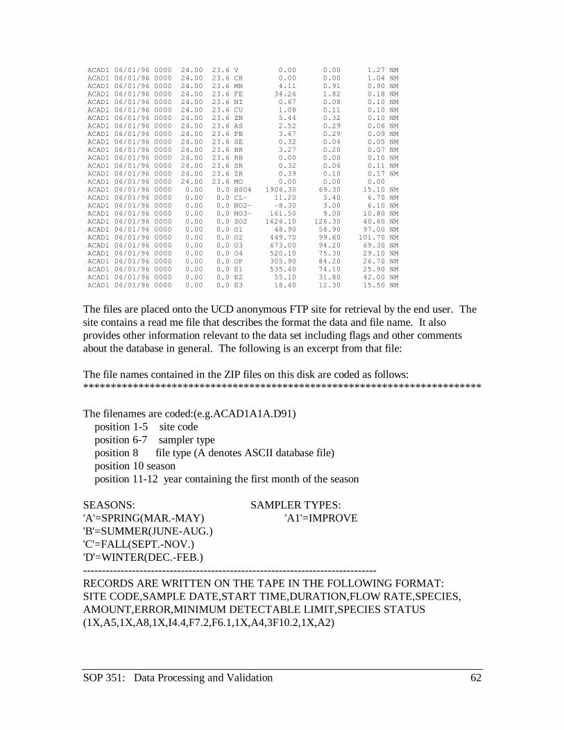
SOP 351: Data Processing and Validation 62
ACAD1 06/01/96 0000 24.00 23.6 V 0.00 0.00 1.27 NM ACAD1 06/01/96 0000 24.00 23.6 CR 0.00 0.00 1.04 NM ACAD1 06/01/96 0000 24.00 23.6 MN 4.11 0.91 0.90 NM ACAD1 06/01/96 0000 24.00 23.6 FE 34.26 1.82 0.18 NM ACAD1 06/01/96 0000 24.00 23.6 NI 0.67 0.08 0.10 NM ACAD1 06/01/96 0000 24.00 23.6 CU 1.08 0.11 0.10 NM ACAD1 06/01/96 0000 24.00 23.6 ZN 5.44 0.32 0.10 NM ACAD1 06/01/96 0000 24.00 23.6 AS 2.52 0.29 0.06 NM ACAD1 06/01/96 0000 24.00 23.6 PB 3.67 0.29 0.09 NM ACAD1 06/01/96 0000 24.00 23.6 SE 0.32 0.04 0.05 NM ACAD1 06/01/96 0000 24.00 23.6 BR 3.27 0.20 0.07 NM ACAD1 06/01/96 0000 24.00 23.6 RB 0.00 0.00 0.10 NM ACAD1 06/01/96 0000 24.00 23.6 SR 0.32 0.06 0.11 NM ACAD1 06/01/96 0000 24.00 23.6 ZR 0.39 0.10 0.17 NM ACAD1 06/01/96 0000 24.00 23.6 MO 0.00 0.00 0.00 ACAD1 06/01/96 0000 0.00 0.0 BSO4 1906.30 69.30 15.10 NM ACAD1 06/01/96 0000 0.00 0.0 CL- 11.20 3.40 6.70 NM ACAD1 06/01/96 0000 0.00 0.0 NO2- -8.30 3.00 6.10 NM ACAD1 06/01/96 0000 0.00 0.0 NO3- 161.50 9.00 10.80 NM ACAD1 06/01/96 0000 0.00 0.0 SO2 1626.10 126.30 40.60 NM ACAD1 06/01/96 0000 0.00 0.0 O1 48.90 58.90 97.00 NM ACAD1 06/01/96 0000 0.00 0.0 O2 449.70 99.60 101.70 NM ACAD1 06/01/96 0000 0.00 0.0 O3 673.00 94.20 69.30 NM ACAD1 06/01/96 0000 0.00 0.0 O4 520.10 75.30 29.10 NM ACAD1 06/01/96 0000 0.00 0.0 OP 305.90 84.20 26.70 NM ACAD1 06/01/96 0000 0.00 0.0 E1 535.40 74.10 25.90 NM ACAD1 06/01/96 0000 0.00 0.0 E2 55.10 31.80 42.00 NM ACAD1 06/01/96 0000 0.00 0.0 E3 18.40 12.30 15.50 NM
The files are placed onto the UCD anonymous FTP site for retrieval by the end user. Thesite contains a read me file that describes the format the data and file name. It alsoprovides other information relevant to the data set including flags and other commentsabout the database in general. The following is an excerpt from that file:
The file names contained in the ZIP files on this disk are coded as follows:************************************************************************
The filenames are coded:(e.g.ACAD1A1A.D91) position 1-5 site code position 6-7 sampler type position 8 file type (A denotes ASCII database file) position 10 season position 11-12 year containing the first month of the season
SEASONS: SAMPLER TYPES:'A'=SPRING(MAR.-MAY) 'A1'=IMPROVE'B'=SUMMER(JUNE-AUG.)'C'=FALL(SEPT.-NOV.)'D'=WINTER(DEC.-FEB.)------------------------------------------------------------------------------RECORDS ARE WRITTEN ON THE TAPE IN THE FOLLOWING FORMAT:SITE CODE,SAMPLE DATE,START TIME,DURATION,FLOW RATE,SPECIES,AMOUNT,ERROR,MINIMUM DETECTABLE LIMIT,SPECIES STATUS(1X,A5,1X,A8,1X,I4.4,F7.2,F6.1,1X,A4,3F10.2,1X,A2)
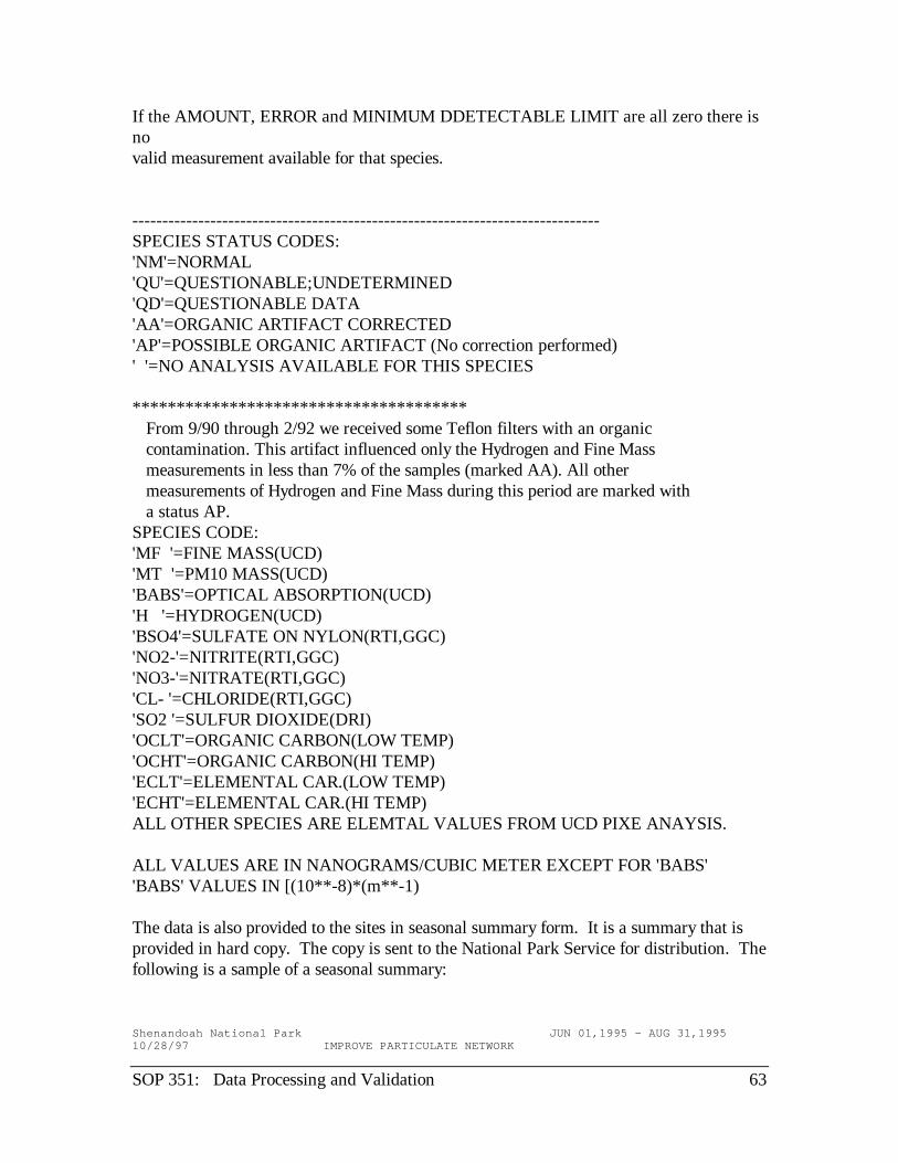
SOP 351: Data Processing and Validation 63
If the AMOUNT, ERROR and MINIMUM DDETECTABLE LIMIT are all zero there isnovalid measurement available for that species.
------------------------------------------------------------------------------SPECIES STATUS CODES:'NM'=NORMAL'QU'=QUESTIONABLE;UNDETERMINED'QD'=QUESTIONABLE DATA'AA'=ORGANIC ARTIFACT CORRECTED'AP'=POSSIBLE ORGANIC ARTIFACT (No correction performed)' '=NO ANALYSIS AVAILABLE FOR THIS SPECIES
************************************** From 9/90 through 2/92 we received some Teflon filters with an organic contamination. This artifact influenced only the Hydrogen and Fine Mass measurements in less than 7% of the samples (marked AA). All other measurements of Hydrogen and Fine Mass during this period are marked with a status AP.SPECIES CODE:'MF '=FINE MASS(UCD)'MT '=PM10 MASS(UCD)'BABS'=OPTICAL ABSORPTION(UCD)'H '=HYDROGEN(UCD)'BSO4'=SULFATE ON NYLON(RTI,GGC)'NO2-'=NITRITE(RTI,GGC)'NO3-'=NITRATE(RTI,GGC)'CL- '=CHLORIDE(RTI,GGC)'SO2 '=SULFUR DIOXIDE(DRI)'OCLT'=ORGANIC CARBON(LOW TEMP)'OCHT'=ORGANIC CARBON(HI TEMP)'ECLT'=ELEMENTAL CAR.(LOW TEMP)'ECHT'=ELEMENTAL CAR.(HI TEMP)ALL OTHER SPECIES ARE ELEMTAL VALUES FROM UCD PIXE ANAYSIS.
ALL VALUES ARE IN NANOGRAMS/CUBIC METER EXCEPT FOR 'BABS''BABS' VALUES IN [(10**-8)*(m**-1)
The data is also provided to the sites in seasonal summary form. It is a summary that isprovided in hard copy. The copy is sent to the National Park Service for distribution. Thefollowing is a sample of a seasonal summary:
Shenandoah National Park JUN 01,1995 - AUG 31,199510/28/97 IMPROVE PARTICULATE NETWORK

SOP 351: Data Processing and Validation 64
Major elements, tracer elements and SO2 24-hour concentrations in nanograms/cubic meter
_______________Soil elements_______________ Smoke DATE HOUR H S SO2 SI K CA TI MN FE KNON06/03/95 0000 295.0 906.0 330 81.7 40.3 25.2 8.3 *1.4 17.7 29.706/07/95 0000 1454.0 4826.0 1626 156.0 58.9 43.3 25.6 *1.9 42.8 33.206/10/95 0000 675.0 2468.0 288 121.3 73.2 23.5 *2.9 7.3 30.2 55.106/14/95 0000 743.0 1386.0 6307 94.3 58.1 32.8 11.9 *1.8 47.2 29.806/17/95 0000 874.0 2311.0 1866 119.0 72.2 33.3 8.9 *1.8 40.8 47.706/21/95 0000 720.0 1579.0 570 86.3 63.4 24.1 *2.9 8.2 24.1 48.906/24/95 0000 263.0 807.0 171 30.5 17.0 7.6 *2.2 *1.4 3.9 14.607/05/95 0000 1223.0 3875.0 269 185.0 63.0 18.7 22.2 *2.2 49.1 33.507/08/95 0000 1072.0 2076.0 1745 87.3 107.2 25.3 *2.2 *1.4 19.9 95.307/12/95 0000 1641.0 3966.0 1283 94.7 77.2 31.0 *3.2 10.3 31.1 58.507/15/95 0000 2208.0 7325.0 3687 304.8 102.0 78.4 30.8 13.2 74.6 57.307/19/95 0000 676.0 1976.0 3511 94.1 38.2 32.6 *2.6 *1.7 28.9 20.807/22/95 0000 1720.0 5870.0 497 117.5 45.5 25.0 21.4 *2.1 27.2 29.107/26/95 0000 825.0 2614.0 356 254.1 43.4 30.5 23.0 3.2 65.6 ?4.107/29/95 0000 638.0 2090.0 537 307.7 55.2 41.0 19.3 *1.7 78.5 ?8.108/16/95 0000 2112.0 7686.0 866 322.6 50.1 53.6 55.8 *3.0 105.3 ?-13.108/19/95 0000 554.0 1041.0 434 96.7 59.0 26.1 8.5 *1.9 31.7 39.908/23/95 0000 1081.0 1739.0 3068 99.7 93.1 32.8 *2.7 *1.8 35.9 71.608/26/95 0000 377.0 1054.0 1887 71.1 31.0 18.8 9.3 *1.4 23.9 16.708/30/95 0000 1023.0 3578.0 1075 127.1 44.8 38.1 29.8 *1.7 59.5 ?9.1
___Marine_____ __________________Metallic tracers___________________ DATE HOUR NA CL- V NI CU ZN AS SE BR PB06/03/95 0000 *25.30 23.2 *1.97 *0.09 0.42 1.97 0.14 0.42 1.28 0.8506/07/95 0000 *62.00 14.6 *2.76 *0.10 0.96 7.59 *0.06 2.04 3.21 3.7306/10/95 0000 *45.80 25.8 11.96 0.72 0.93 4.80 *0.06 0.77 2.35 2.6906/14/95 0000 65.00 27.0 *2.64 0.47 1.49 13.03 *0.07 1.28 3.78 4.3006/17/95 0000 *42.90 34.5 *2.66 0.44 1.26 8.85 *0.06 1.52 3.91 3.3706/21/95 0000 *34.80 26.6 *2.61 *0.10 1.08 5.05 *0.06 0.93 2.71 1.8706/24/95 0000 57.00 23.5 *2.00 *0.08 0.34 1.16 *0.05 0.32 0.83 1.0007/05/95 0000 ?37.40 18.2 *3.11 0.39 1.15 4.23 *0.07 1.91 2.76 2.6007/08/95 0000 *35.70 17.5 *2.06 *0.09 1.13 11.25 *0.06 1.79 3.34 2.8307/12/95 0000 *58.20 34.1 *2.87 *0.10 1.97 11.72 *0.07 2.02 4.32 4.0207/15/95 0000 *100.80 13.4 *3.87 *0.13 1.74 10.98 *0.08 3.24 4.64 5.1307/19/95 0000 *37.10 23.7 *2.39 *0.09 1.12 9.49 *0.06 1.25 1.94 3.4707/22/95 0000 *75.20 14.4 *3.06 0.69 1.29 6.45 *0.07 2.54 2.85 3.3907/26/95 0000 *43.60 14.4 *2.31 *0.09 1.31 2.84 *0.05 1.06 1.08 1.8107/29/95 0000 62.60 28.5 *2.52 0.17 0.80 4.06 *0.05 0.86 1.64 1.9408/16/95 0000 ?46.20 ?3.6 *4.32 1.53 1.88 13.88 *0.09 2.81 3.86 7.1808/19/95 0000 142.70 74.7 *2.78 0.79 0.97 3.87 *0.06 0.79 3.54 2.4908/23/95 0000 42.70 35.3 6.28 *0.10 3.45 10.20 *0.07 1.26 4.04 3.8208/26/95 0000 121.70 43.8 *2.02 0.39 0.82 4.32 0.36 0.74 2.68 1.8308/30/95 0000 *50.80 16.5 ?5.27 *0.13 1.53 13.92 *0.08 1.55 3.08 5.68
*=minimum detectable limit ?= < (2 x uncertainty) #= MASS>PM10; diff<uncertainty
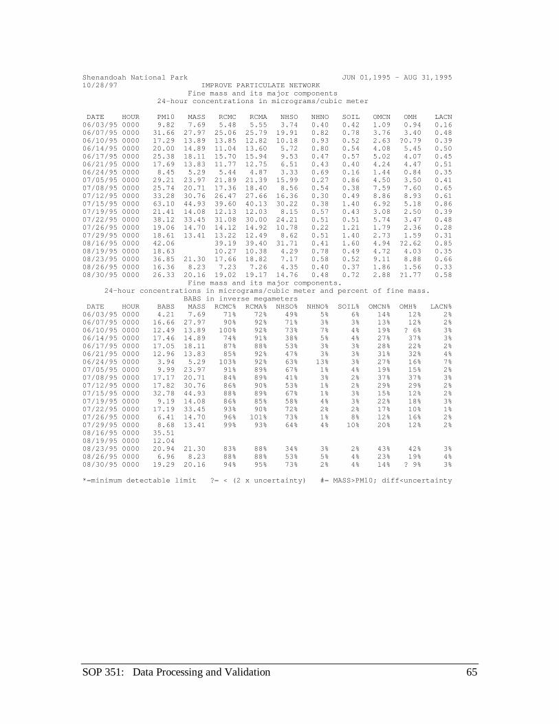
SOP 351: Data Processing and Validation 65
Shenandoah National Park JUN 01,1995 - AUG 31,199510/28/97 IMPROVE PARTICULATE NETWORK Fine mass and its major components 24-hour concentrations in micrograms/cubic meter
DATE HOUR PM10 MASS RCMC RCMA NHSO NHNO SOIL OMCN OMH LACN06/03/95 0000 9.82 7.69 5.48 5.55 3.74 0.40 0.42 1.09 0.94 0.1606/07/95 0000 31.66 27.97 25.06 25.79 19.91 0.82 0.78 3.76 3.40 0.4806/10/95 0000 17.29 13.89 13.85 12.82 10.18 0.93 0.52 2.63 ?0.79 0.3906/14/95 0000 20.00 14.89 11.04 13.60 5.72 0.80 0.54 4.08 5.45 0.5006/17/95 0000 25.38 18.11 15.70 15.94 9.53 0.47 0.57 5.02 4.07 0.4506/21/95 0000 17.69 13.83 11.77 12.75 6.51 0.43 0.40 4.24 4.47 0.5106/24/95 0000 8.45 5.29 5.44 4.87 3.33 0.69 0.16 1.44 0.84 0.3507/05/95 0000 29.21 23.97 21.89 21.39 15.99 0.27 0.86 4.50 3.50 0.4107/08/95 0000 25.74 20.71 17.36 18.40 8.56 0.54 0.38 7.59 7.60 0.6507/12/95 0000 33.28 30.76 26.47 27.66 16.36 0.30 0.49 8.86 8.93 0.6107/15/95 0000 63.10 44.93 39.60 40.13 30.22 0.38 1.40 6.92 5.18 0.8607/19/95 0000 21.41 14.08 12.13 12.03 8.15 0.57 0.43 3.08 2.50 0.3907/22/95 0000 38.12 33.45 31.08 30.00 24.21 0.51 0.51 5.74 3.47 0.4807/26/95 0000 19.06 14.70 14.12 14.92 10.78 0.22 1.21 1.79 2.36 0.2807/29/95 0000 18.61 13.41 13.22 12.49 8.62 0.51 1.40 2.73 1.59 0.3108/16/95 0000 42.06 39.19 39.40 31.71 0.41 1.60 4.94 ?2.62 0.8508/19/95 0000 18.63 10.27 10.38 4.29 0.78 0.49 4.72 4.03 0.3508/23/95 0000 36.85 21.30 17.66 18.82 7.17 0.58 0.52 9.11 8.88 0.6608/26/95 0000 16.36 8.23 7.23 7.26 4.35 0.40 0.37 1.86 1.56 0.3308/30/95 0000 26.33 20.16 19.02 19.17 14.76 0.48 0.72 2.88 ?1.77 0.58 Fine mass and its major components. 24-hour concentrations in micrograms/cubic meter and percent of fine mass. BABS in inverse megameters DATE HOUR BABS MASS RCMC% RCMA% NHSO% NHNO% SOIL% OMCN% OMH% LACN%06/03/95 0000 4.21 7.69 71% 72% 49% 5% 6% 14% 12% 2%06/07/95 0000 16.66 27.97 90% 92% 71% 3% 3% 13% 12% 2%06/10/95 0000 12.49 13.89 100% 92% 73% 7% 4% 19% ? 6% 3%06/14/95 0000 17.46 14.89 74% 91% 38% 5% 4% 27% 37% 3%06/17/95 0000 17.05 18.11 87% 88% 53% 3% 3% 28% 22% 2%06/21/95 0000 12.96 13.83 85% 92% 47% 3% 3% 31% 32% 4%06/24/95 0000 3.94 5.29 103% 92% 63% 13% 3% 27% 16% 7%07/05/95 0000 9.99 23.97 91% 89% 67% 1% 4% 19% 15% 2%07/08/95 0000 17.17 20.71 84% 89% 41% 3% 2% 37% 37% 3%07/12/95 0000 17.82 30.76 86% 90% 53% 1% 2% 29% 29% 2%07/15/95 0000 32.78 44.93 88% 89% 67% 1% 3% 15% 12% 2%07/19/95 0000 9.19 14.08 86% 85% 58% 4% 3% 22% 18% 3%07/22/95 0000 17.19 33.45 93% 90% 72% 2% 2% 17% 10% 1%07/26/95 0000 6.41 14.70 96% 101% 73% 1% 8% 12% 16% 2%07/29/95 0000 8.68 13.41 99% 93% 64% 4% 10% 20% 12% 2%08/16/95 0000 35.5108/19/95 0000 12.0408/23/95 0000 20.94 21.30 83% 88% 34% 3% 2% 43% 42% 3%08/26/95 0000 6.96 8.23 88% 88% 53% 5% 4% 23% 19% 4%08/30/95 0000 19.29 20.16 94% 95% 73% 2% 4% 14% ? 9% 3%
*=minimum detectable limit ?= < (2 x uncertainty) #= MASS>PM10; diff<uncertainty

SOP 351: Data Processing and Validation 66
Shenandoah National Park JUN 01,1995 - AUG 31,199510/28/97 IMPROVE PARTICULATE NETWORK
Distribution of Concentrations in nanograms/cubic meter
% of cases Arithmetic Maximum Cases Significant Mean Minimum Median Maximum occursH 20 100% 1008.70 262.99 849.49 2208.34 07/15/95S 20 100% 2958.61 807.17 2200.27 7686.11 08/16/95SO2 20 100% 1518.65 171.30 970.70 6306.60 06/14/95SI 20 100% 142.58 30.45 108.62 322.59 08/16/95K 20 100% 59.64 16.95 58.53 107.22 07/08/95CA 20 100% 32.08 7.62 30.73 78.40 07/15/95TI 20 65% 14.67 2.15 9.11 55.82 08/16/95MN 20 25% 3.46? 1.37 1.88? 13.16 07/15/95FE 20 100% 41.90 3.88 33.81 105.32 08/16/95KNON 20 85% 34.50 -13.08 31.53 95.27 07/08/95NA 20 30% 59.38? 25.25 48.53? 142.69 08/19/95CL- 20 95% 25.67 3.60 23.60 74.70 08/19/95V 20 10% 3.47? 1.97 2.71? 11.96 06/10/95NI 20 45% 0.33? 0.08 0.13? 1.53 08/16/95CU 20 100% 1.28 0.34 1.14 3.45 08/23/95ZN 20 100% 7.48 1.16 7.02 13.92 08/30/95AS 20 10% 0.08? 0.05 0.07? 0.36 08/26/95SE 20 100% 1.46 0.32 1.27 3.24 07/15/95BR 20 100% 2.89 0.83 2.97 4.64 07/15/95PB 20 100% 3.20 0.85 3.10 7.18 08/16/95
Distribution of Concentrations in micrograms/cubic meter
% of cases Arithmetic Maximum Cases Significant Mean Minimum Median Maximum occursPM10 20 100% 25.95 8.45 23.40 63.10 07/15/95
MASS 18 100% 19.30 5.29 16.50 44.93 07/15/95RCMC 20 100% 17.88 5.44 14.91 39.60 07/15/95RCMA 20 100% 18.17 4.87 15.43 40.13 07/15/95NHSO 20 100% 12.20 3.33 9.08 31.71 08/16/95NHNO 20 100% 0.52 0.22 0.50 0.93 06/10/95SOIL 20 100% 0.69 0.16 0.52 1.60 08/16/95OMCN 20 100% 4.35 1.09 4.16 9.11 08/23/95OMH 20 85% 3.70 0.79 3.44 8.93 07/12/95LACN 20 100% 0.48 0.16 0.47 0.86 07/15/95
Distribution of Concentrations in micrograms/cubic meter and percent of fine mass BABS in inverse megameters
% of cases Arithmetic Maximum Cases Significant Mean Minimum Median Maximum occursBABS 20 100% 14.94 3.94 14.81 35.51 08/16/95MASS 18 100% 19.30 5.29 16.50 44.93 07/15/95RCMC% 18 100% 89% 71% 88% 103% 06/24/95RCMA% 18 100% 90% 72% 90% 101% 07/26/95NHSO% 18 100% 58% 34% 60% 73% 07/26/95NHNO% 18 100% 4% 1% 3% 13% 06/24/95SOIL% 18 100% 4% 2% 3% 10% 07/29/95OMCN% 18 100% 23% 12% 21% 43% 08/23/95OMH% 18 88% 20% 6% 16% 42% 08/23/95LACN% 18 100% 3% 1% 3% 7% 06/24/95
A significant value is greater than 2 times the uncertainty of that value.
?=the percentage of significant values is less than 65%