Impact of Lumping Techniques for Fluid Characterization in...

Australian Journal of Basic and Applied Sciences, 7(1): 320-333, 2013 ISSN 1991-8178

Corresponding Author: Hamidreza moghadamzadeh, Islamic Azad University South Tehran Branch, P.O. Box 19585-466, Tehran, Iran

E-mail: [email protected] 320

Impact of Lumping Techniques for Fluid Characterization in Gas Condensate Reservoir

1Hamidreza moghadamzadeh, 2Hojjatolla Maghsoodloorad, 3Adel zarabpour, 2,4Ali Hemmati, 5Shahin

Shahsavari, 6Shadab Shahsavari

1Islamic Azad University South Tehran Branch, P.O. Box 19585-466, Tehran, Iran 2School of Chemical Engineering, Iran University of Science and Technology (IUST), Narmak,

Tehran, Iran 3Islamic Azad University Tabas Branch, 4-police University

5Department of Chemical Engineering, University of Sistan and Baluchestan, Zahedan, Iran 6Department of Chemical Engineering, Varamin (Pishva) Branch, Islamic Azad University, Tehran,

Iran

Abstract: Several problems are associated with “regrouping” the original components into a smaller number without losing the predicting power of the equation of state. These problems include (A) How to select the groups of pure components to be represented by one pseudo-component. (B) What mixing rules should be used for determining the EOS constants (pc, Tc, and ω) for the new lumped pseudo-components? In this paper the results of the lumping methods are compared with the data for gas condensate systems to find accurate lumping method for accurate fluid characterization. For this purpose, Whitson’s lumping scheme, Pedersen lumping scheme, Danesh et al. lumping scheme, Lee et al. lumping scheme, Behras and Stanndler lumping scheme are used as lumping scheme and Lee mixing rules was used for calculation of thermodynamics properties of lumped group. To compare the Impact of each Lumping method, its effect was examined on the phase diagram. The results show that the Whitson lumping scheme (it is grouping the hydrocarbon from C7 to C16+ into 4 groups) can predict the phase diagram of this gas condensate systems fluid with good approximation, the Pedersen lumping scheme (it is grouping the hydrocarbon from C7 to C16+ into 3 groups ) can predict the phase diagram of this gas condensate systems fluid somewhat and the Pedersen lumping schemes and Danesh et al. lumping schemes (it is grouping the hydrocarbon from C7 to C16+ into 4 groups) approximately predicted the same phase diagram and the Lee et al. lumping scheme (it is grouping the hydrocarbon from C7 to C16+ into 3 groups) can predict the phase diagram of this gas condensate systems fluid exactly. Therefore, the Lee at al. lumping scheme has very good accuracy compared to the other methods. Also, All Lumping Scheme has an effect on dew point line of phase diagram. Key words: Lumping, Groping, Pseudoization, Pseudo component, Mixing rule.

INTRODUCTION

Petroleum is composed of various hydrocarbon and non-hydrocarbon components. For characterizing and

simulating the oil reservoir, the reservoir fluid must be characterized. The large number of components is necessary to describe the hydrocarbon mixture for accurate phase behavior modeling frequently burdens EOS calculations.

Generally, with a sufficiently large number of pseudo-components used in characterizing the heavy fraction of a hydrocarbon mixture, a satisfactory prediction of the PVT behavior by the equation of state can be obtained. However the cost and computing time can be increased significantly with the increased number of components in the system. Therefore, strict limitations are placed on the maximum number of components that can be used in compositional models and the original components have to be lumped into a smaller number of pseudo components (Ahmed 2010, 1989).

Several problems are associated with “regrouping” the original components into a smaller number without losing the predicting power of the equation of state. These problems include How to select the groups of pure components to be represented by one pseudo-component each.

Several unique techniques have been published that can be used to address the above lumping problems; notably the methods proposed by Mehra et al, Schlijper, Gonzalez, Colonomos, and Rusinek, Aguilar and McCain, Pedersen et al. (Ahmed 2010, 1989; Hong 1982; Guo and Du 1989; Lee et al. 1981; Montel and Gouel 1984; Al-Meshari 2004), Whitson (Whitson 1983), Lee et al. (Lee et al. 1981), Montel and Gouel (Montel and Gouel 1984), Behrens and Sandler (Behrens and Sandler 1988), Hong (Hong 1982) and Danesh et al. (Danesh et al. 1992).

Aust. J. Basic & Appl. Sci., 7(1): 320-333, 2013

321

For describing the phase behavior of a fluid mixture, critical pressure, critical temperature, critical volume, acentric factor, molecular weight and binary interaction parameters of component must be specified. Different mixing rules were evaluated for, characterizing the lumped C7+ fraction from its constituent component properties (Ahmed 2010; Hong 1982; Adepoju 2006; Joergensen and Stenby 1995).

Impact of these lumping schemes on one system, especially gas condensate systems, isn’t studied. In this work, the accuracy and impact of Whitson, Pedersen, Danesh et al., Lee et al., Behras and stanndler lumping scheme on phase diagram of the gas condensate systems are researched. Lee’s mixing rule is one of these mixing rules which are used in this research. 2. Methods: 2.1 Experiment:

A sample of reservoir fluid is prepared from one of gas condensate oil fields. In the laboratory, it composition is determined by using gas chromatography. Also, the properties of heavy oil fraction were measured with the existing standards methods in the laboratory. 2.2 Lee’s mixing rules:

There are many mixing rules which obtained by researchers. Lee’s mixing rules is one of useful rules. Lee et al. (1979) (Ahmed 2010) used Kay’s mixing rules as the characterizing approach for determining the properties of the lumped fractions in their suggested regrouping model. To using this rule, normalized mole fraction of the component i in the lumped fraction must be defined. It was defined by:

∑= L

i

ii

z

zφ (1)

After that, Lee et al. are proposed the following rules for calculation of thermodynamic property of multi component mixture:

(2)

∑= L

ii

LL

Mw

Mw

φγ

(3)

∑=L

ciiicL Mw

VMwV

φ (4)

∑=L

ciicl PP φ (5)

∑=L

ciicL TT φ (6)

∑=L

iil ωφω (7)

3. Results: In this paper, Whitson’s lumping scheme, Pedersen lumping scheme, Danesh et al. lumping scheme, Lee et

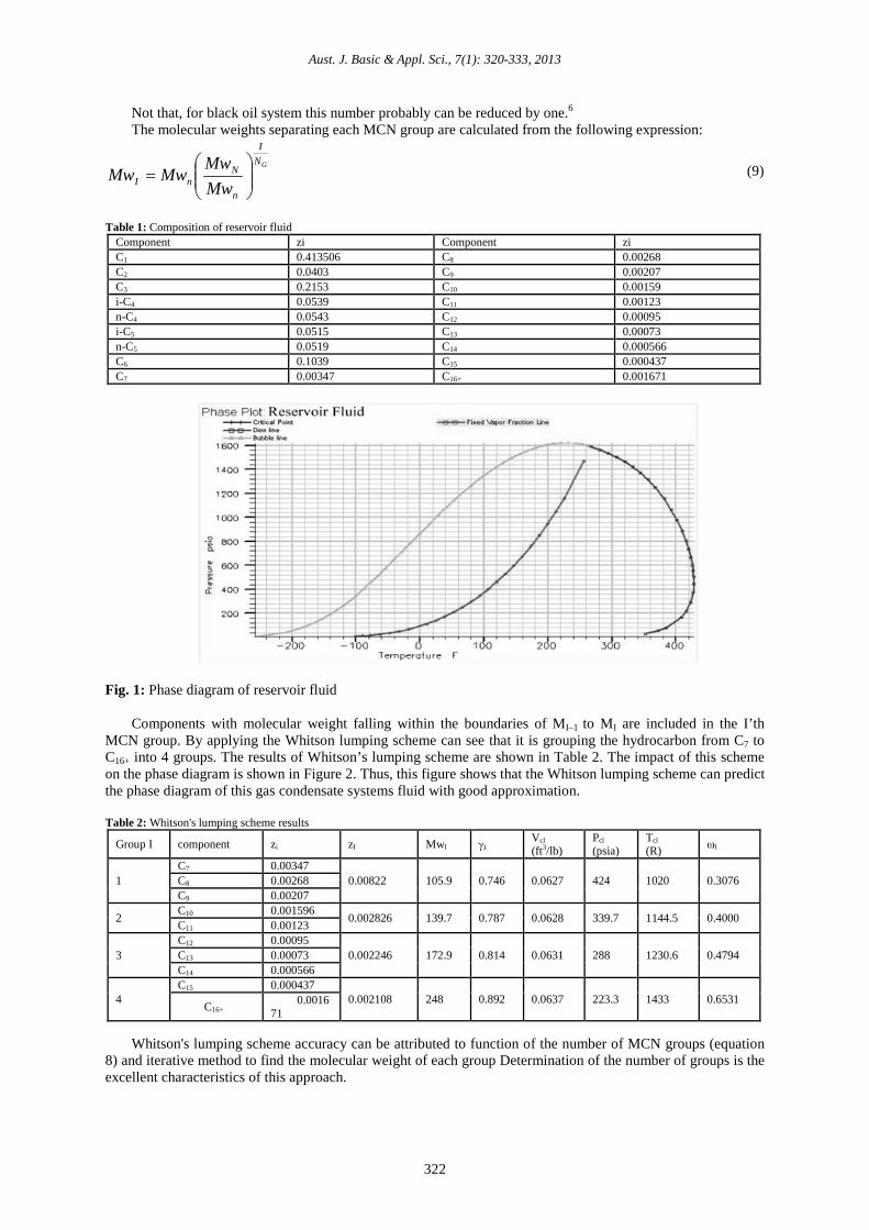
al. lumping scheme, Behras and Stanndler lumping scheme are used. Calculation of the method described in the appendix. A compositional analysis of gas condensate systems fluid described in Table 1 and the molecular weight and the specific gravity of C16+ is equal to 259 and 0.908 respectively. The phase diagram of this gas condensate system is shown in Figure 1.

3.1 Whitson’s lumping scheme:

Whitson (Whitson 1983) proposed a regrouping scheme whereby the compositional distribution of the C7+ fraction is reduced to only a few multiple carbon- number (MCN) groups. Whitson suggested that the number of MCN groups is necessary to describe the plus fraction is given by the following empirical rule:

( )[ ]nNIntNG −+= log3.31 (8)


322

Not that, for black oil system this number probably can be reduced by one.6

The molecular weights separating each MCN group are calculated from the following expression:

GNI

n

NnI Mw

MwMwMw

= (9)

Table 1: Composition of reservoir fluid

Component zi Component zi C1 0.413506 C8 0.00268 C2 0.0403 C9 0.00207 C3 0.2153 C10 0.00159 i-C4 0.0539 C11 0.00123 n-C4 0.0543 C12 0.00095 i-C5 0.0515 C13 0.00073 n-C5 0.0519 C14 0.000566 C6 0.1039 C15 0.000437 C7 0.00347 C16+ 0.001671

Fig. 1: Phase diagram of reservoir fluid

Components with molecular weight falling within the boundaries of MI–1 to MI are included in the I’th MCN group. By applying the Whitson lumping scheme can see that it is grouping the hydrocarbon from C7 to C16+ into 4 groups. The results of Whitson’s lumping scheme are shown in Table 2. The impact of this scheme on the phase diagram is shown in Figure 2. Thus, this figure shows that the Whitson lumping scheme can predict the phase diagram of this gas condensate systems fluid with good approximation.

Table 2: Whitson's lumping scheme results

Group I component zi zI MwI γI Vcl (ft3/lb)

Pcl (psia)

Tcl (R) ωl

1 C7 0.00347

0.00822 105.9 0.746 0.0627 424 1020 0.3076 C8 0.00268 C9 0.00207

2 C10 0.001596 0.002826 139.7 0.787 0.0628 339.7 1144.5 0.4000 C11 0.00123

3 C12 0.00095

0.002246 172.9 0.814 0.0631 288 1230.6 0.4794 C13 0.00073 C14 0.000566

4 C15 0.000437

0.002108 248 0.892 0.0637 223.3 1433 0.6531 C16+ 0.0016

71 Whitson's lumping scheme accuracy can be attributed to function of the number of MCN groups (equation

8) and iterative method to find the molecular weight of each group Determination of the number of groups is the excellent characteristics of this approach.


323

Fig. 2: Impact of Whitson’s lumping scheme on phase diagram 3.2 Pedersen Lumping Scheme:

Pedersen et al. (Ahmed 2010, 1989; Hong 1982; Guo and Du 1989; Lee et al. 1981; Montel and Gouel 1984; Al-Meshari 2004) suggested the process of grouping the components on the basis of each group containing approximately the same weight fraction (equal weight fraction), which will give all hydrocarbon segments of the C7+ fractions equal importance. The C7+ fraction is divided into three or more groups that, by weight, are equal size approximately. The weight for each pseudo component, Wj, can be calculated as:

∑=

×=cn

iiij Mwzw

1

(10)

By applying the Pedersen lumping scheme can see that it is grouping the hydrocarbon from C7 to C16+ into 3 groups (3 groups is selected according to some restrictions). The results of Pedersen lumping scheme are shown in Table 3. The phase diagram of this system is under the impact of Pedersen lumping scheme is shown in Figure 3. Therefore, this figure shows that the Pedersen lumping scheme can predict the phase diagram of this gas condensate systems fluid somewhat.

Table 3: Pedersen lumping scheme results

Group I component zi zI MwI γI Vcl (ft3/lb)

Pcl (psia)

Tcl

(R) ωl

1 C7 0.00347 0.00615 100.794 0.73657 0.06277 438.184 1007.2 0.29395 C8 0.00268

2

C9 0.00207

0.00584 136.522 0.78409 0.06279 348.896 1123.4 0.39027 C10 0.001596 C11 0.00123 C12 0.00095

3

C13 0.00073

0.003404 222.709 0.86866 0.06353 244.507 1363.8 0.59401 C14 0.000566 C15 0.000437 C16+ 0.001671

As you can see, a simple relationship exists between the concentration and molecular weight in Pedersen

lumping scheme. Choosing the number of groups is based on the limitations and experiences, so, the accuracy of this method would not be high.

3.3 Danesh et al. lumping scheme:

Danesh et al. (Danesh et al. 1992) proposed a lumping method based on the concentration and molecular weight of compounds in a mixture. This grouping method arranged the original components in order of their normal boiling point temperatures and grouped together in ascending order to form Np groups so that the values of Σ (zilnMi) for all the groups become nearly equal, (Quasi-equal-weight criterion). That is:

0ln1ln11

≤

××

−× ∑∑

==

n

iii

pi

l

ii Mwz

NMwz (11)

And


324

p

l

i

n

iii

pii

Nlni

MwzN

Mwz

,...2,1,,...,2,1

0ln1ln1

1 1

==

≥

×

−∑ ∑

+

= = (12)

Fig. 3: Impact of Pedersen lumping scheme on phase diagram

According to the Danesh et al. lumping scheme can see that it is grouping the hydrocarbon from C7 to C16+

into 4 groups. The results of Danesh et al. lumping scheme are shown in Table 4. The phase diagram of this system is under the impact of Danesh et al. lumping scheme is shown in Figure 4. The predicted phase diagram of this gas condensate systems fluid by the Danesh et al. lumping scheme is look like the phase diagram was predicted by Pedersen lumping scheme. Figure 4 show that this lumping scheme can predict the phase diagram somewhat.

In this method, choosing the number of groups was done similar to the Pedersen lumping scheme. In Danesh et al. lumping scheme some limitation is defined for choosing the molecular weight of groups, so it would be more accurate than the Pedersen lumping scheme.

Table 4: Danesh et al. lumping scheme results

Group I component zi zI MwI γI

Vcl (ft3/lb)

Pcl (psia)

Tcl

(R) ωl

1 C7 0.00347 0.00347 96 0.727 0.06289 453 985 96

2 C8 C9

0.00268 0.00207 0.00475 113.101 0.75719 0.06261 403.312 1045.59 113.101

3 C10 C11 C12

0.001596 0.00123 0.00095

0.00377 145.045 0.79169 0.06288 330.17 1159.3 145.045

4

C13 0.00073

0.003404 222.709 0.86866 0.06353 244.507 1363.78 222.709 C14 0.000566 C15 0.000437 C16+ 0.001671

3.4 Lee et al. lumping scheme:

Lee et al. (Lee et al. 1981) devised a simple procedure that can be served as a guideline for lumping the oil fractions. The idea for the procedure lies in the physical reasoning that crude-oil fractious having relatively close physicochemical properties can be represented fairly accurately by a single fraction, the closeness of these properties can be reflected by the slopes of curve when these properties are plotted against some characteristic independent variables.

According to the Lee et al. lumping scheme can see that it is grouping the hydrocarbon from C7 to C16+ into 3 groups. The results of Lee et al. lumping scheme are shown in Table 5. The accuracy of this scheme can be seen in the phase diagram in Figure 5. Hence, Figure 5 shows that the Lee et al. lumping scheme can predict the phase diagram of this gas condensate systems fluid exactly.


325

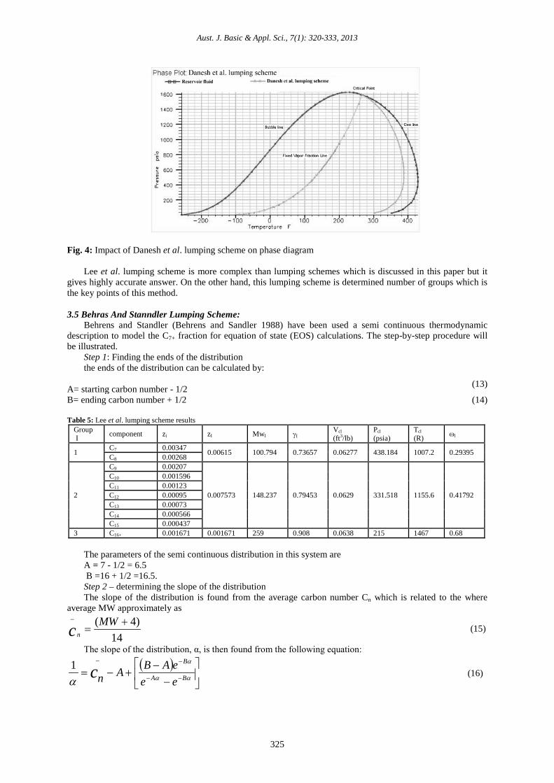
Fig. 4: Impact of Danesh et al. lumping scheme on phase diagram

Lee et al. lumping scheme is more complex than lumping schemes which is discussed in this paper but it

gives highly accurate answer. On the other hand, this lumping scheme is determined number of groups which is the key points of this method. 3.5 Behras And Stanndler Lumping Scheme:

Behrens and Standler (Behrens and Sandler 1988) have been used a semi continuous thermodynamic description to model the C7+ fraction for equation of state (EOS) calculations. The step-by-step procedure will be illustrated.

Step 1: Finding the ends of the distribution the ends of the distribution can be calculated by:

A= starting carbon number - 1/2 (13)

B= ending carbon number + 1/2 (14) Table 5: Lee et al. lumping scheme results

Group I component zi zI MwI γI

Vcl (ft3/lb)

Pcl (psia)

Tcl

(R) ωl

1 C7 0.00347 0.00615 100.794 0.73657 0.06277 438.184 1007.2 0.29395 C8 0.00268

2

C9 0.00207

0.007573 148.237 0.79453 0.0629 331.518 1155.6 0.41792

C10 0.001596 C11 0.00123 C12 0.00095 C13 0.00073 C14 0.000566 C15 0.000437

3 C16+ 0.001671 0.001671 259 0.908 0.0638 215 1467 0.68

The parameters of the semi continuous distribution in this system are A = 7 - 1/2 = 6.5 B =16 + 1/2 =16.5. Step 2 – determining the slope of the distribution The slope of the distribution is found from the average carbon number Cn which is related to the where

average MW approximately as

14)4( +

=− MW

nc (15)

The slope of the distribution, α, is then found from the following equation:

( )

−

−+−= −−

−−

αα

α

α BA

B

eeeABAnc1

(16)


326

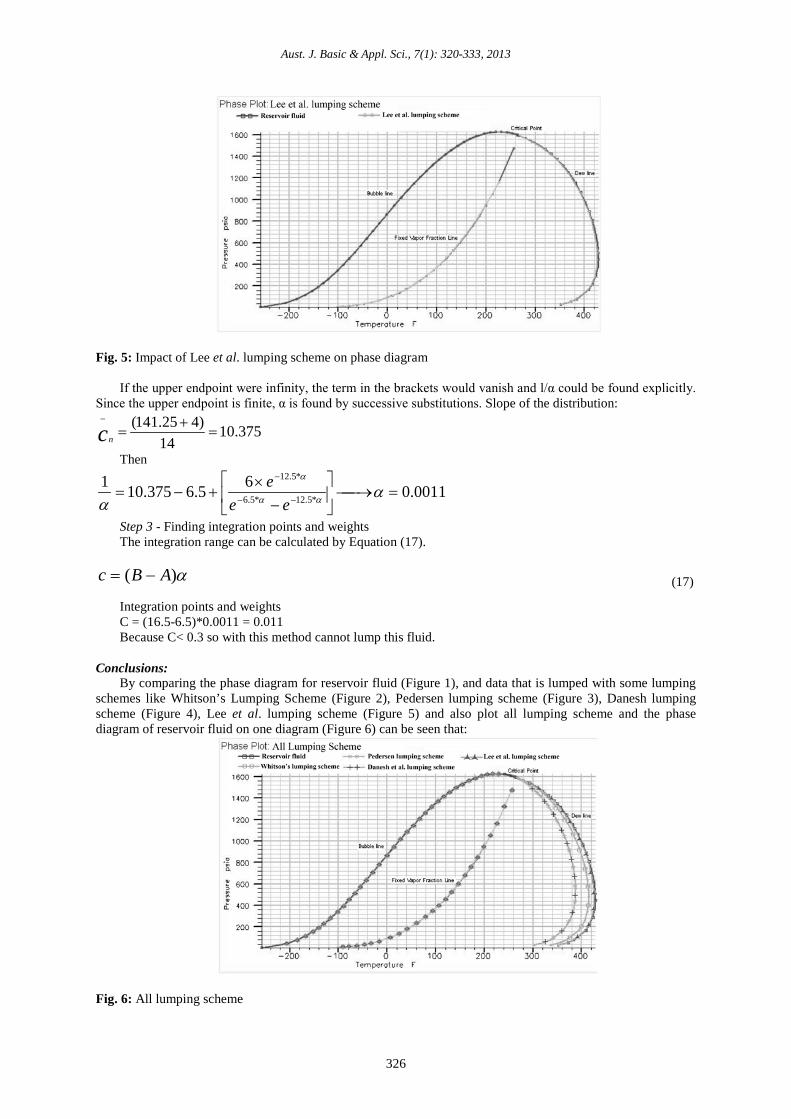
Fig. 5: Impact of Lee et al. lumping scheme on phase diagram

If the upper endpoint were infinity, the term in the brackets would vanish and l/α could be found explicitly.

Since the upper endpoint is finite, α is found by successive substitutions. Slope of the distribution:

375.1014

)425.141(=

+=

−

nc

Then

0011.065.6375.101*5.12*5.6

*5.12

=→

−

×+−= −−

−

αα αα

α

eee

Step 3 - Finding integration points and weights The integration range can be calculated by Equation (17).

α)( ABc −= (17)

Integration points and weights C = (16.5-6.5)*0.0011 = 0.011 Because C< 0.3 so with this method cannot lump this fluid.

Conclusions:

By comparing the phase diagram for reservoir fluid (Figure 1), and data that is lumped with some lumping schemes like Whitson’s Lumping Scheme (Figure 2), Pedersen lumping scheme (Figure 3), Danesh lumping scheme (Figure 4), Lee et al. lumping scheme (Figure 5) and also plot all lumping scheme and the phase diagram of reservoir fluid on one diagram (Figure 6) can be seen that:

Fig. 6: All lumping scheme


327

1- With the Pedersen Lumping Scheme and Danesh et al. Lumping Scheme can reach to the approximately same the phase diagram. 2- Lee at al. Lumping Scheme has very good accuracy related to the other methods in characterization of gas condensate reservoir. 3- All Lumping Scheme has an effect on dew point line.

REFERENCES

Adepoju, O.O., 2007. Coefficient of Isothermal Oil Compressibility- A Study for Reservoir Fluids by Cubic

Equation-of-State. VDM Verlag Dr. Mueller e.K Press. Ahmed, T.H., 1989. Hydrocarbon phase behavior, Contributions in petroleum geology & engineering 7.

Gulf Pub. Co Press. Ahmed, Tarek H., 2010. Reservoir engineering handbook. Gulf Professional Pub Press. Al-Meshari, A.A., 2004. New strategic method to tune equation-of-state to match experimental data for

compositional simulation, Ph.D. thesis, Texas A&M University, Texas Behrens, R.A., and S.I. Sandler, 1988. The Use of Semicontinuous Description To Model the C7+ Fraction

in Equation of State Calculations. SPE Reservoir Engineering, 3(3): 1041-1047. Danesh, Ali, Dong-hai Xu, Adrian C. Todd, and U. Heriot-Watt, 1992. A Grouping Method To Optimize

Oil Description for Compositional Simulation of Gas-Injection Processes. SPE Reservoir Engineering, 7(3): 343-348.

Guo, T.M., and L. and Du., 1989. A New Three Parameter Cubic Equation of State for Reservoir Fluids–Part II. Application to Reservoir Crude Oils. SPE pp: 19373.

Hong, K.C., 1982. Lumped-Component Characterization of Crude Oils for Compositional Simulation. In SPE Enhanced Oil Recovery Symposium, Tulsa, Oklahoma

Joergensen, M., and E.H. Stenby, 1995. Optimization of Pseudo-component Selection for Compositional Studies of Reservoir Fluids. In 70th Annul Technical Conference and Exhibition. Daltas, Taxas.

Lee, S.T., R.H. Jacoby, W.H. Chen, W.E. Culham, and Gulf Research and Development Co., 1981. Experimental and Theoretical Studies on the Fluid Properties Required for Simulation of Thermal Processes. SPE Journal., 21(5): 535-550.

Montel, F., and P.L. Gouel., 1984. A New Lumping Scheme of Analytical Data for Compositional Studies. In SPE Annual Technical Conference and Exhibition. Houston, Texas.

Whitson, C., 1983. Characterizing Hydrocarbon Plus Fractions. SPE Journal, 23(4): 683-694.

Nomanclature: I = 1, 2. . . Ng i = component i Int = integer L = lumped fraction MwC7 = molecular weight of C7 Mwi = Molecular weight MwN+ = molecular weight of the last reported component in the extended analysis of the hydrocarbon

system n = number of carbon atoms of the first component in the plus fraction, i.e., n = 7 for C7+ N = number of carbon atoms of the last component in the hydrocarbon system Ng = number of MCN groups Pci = Critical pressure Tci = Critical temperature vci = Critical volume Wj = weight for each pseudo component Zi = mole fraction Фi = weighting factor ωi = Acentric factor

Appendix A: A.1 Whitson’s lumping scheme:

Determining the appropriate number of pseudo-components forming in the C7+ by using the Whitson’s Lumping Scheme

Step 1. Determining the molecular weight of each component in the system:


328

TableA-1: Molecular weight of components component zi Mwi C7 0.00347 96 C8 0.00268 107 C9 0.00207 121 C10 0.00159 134 C11 0.00123 147 C12 0.00095 161 C13 0.00073 175 C14 0.000566 190 C15 0.000437 206 C16+ 0.001671 259

Step 2. Calculating the number of pseudo-components: For calculation of pseudo-components having N=16 n=7

[ ])log(3.31 nNIntNg −+=

Therefore,

[ ])716log(3.31 −+= IntNg [ ]15.4IntNg =

4=gN

Step 3. Determining the molecular weights separating the hydrocarbon groups:

gNI

C

NCI Mw

MwMwMw

= +

77

4

9625996

I

IMw

=

Therefore,

( ) 4698.296I

IMw =

Table A-2: Molecular weight of each group I MWI

1 123.0359 2 157.6857 3 202.0937 4 259.008

• First pseudo-component: The first pseudo-component includes all components with a molecular weight

in the range of 96 to 123. This group then includes C7, C8, and C9. • Second pseudo-component: The second pseudo-component contains all components with a molecular

weight higher than 123 to a molecular weight of 158. This group includes C10 and C11. • Third pseudo-component: The third pseudo-component includes components with a molecular weight

higher than 158 to a molecular weight of 202. Therefore, this group includes C12, C13, and C14. • Fourth pseudo-component: This pseudo-component includes all the remaining components, i.e., C15 and

C16+. Table A-3: Molecular percentofeach group

Group I component zi zI

1 C7 0.00347

0.00822 C8 0.00268 C9 0.00207

2 C10 0.001596 0.002826


329

C11 0.00123

3 C12 0.00095

0.002246 C13 0.00073 C14 0.000566

4 C15 0.000437 0.002108 C16+ 0.001671 Zl is calculated by the equation of:

l

l

i zz =∑

there are numerous ways to mix the properties of the individual components, all giving different properties for the pseudo-components, the choice of a correct mixing rule is as important as the lumping scheme.

The mixing rules can be employed to characterize the pseudo-component in terms of its pseudo physical and pseudo-critical properties. In this Example Using Lee’s mixing rules to determine the physical and critical properties of the four pseudo-components TableA-4: Thermodynamics property of components


Mwi from appendix

γi

from appendix

vci from appendix

Pci from appendix

Tci from appendix

ωi from appendix

1 C7 0.00347

0.00822 96 0.727 0.06289 453 985 0.280

C8 0.00268 107 0.748 0.06264 419 1036 0.312 C9 0.00207 121 0.768 0.06258 383 1058 0.348

2 C10 0.001596 0.002826 134 0.782 0.06273 351 1128 0.385 C11 0.00123 147 0.793 0.06291 325 1166 0.419

3 C12 0.00095

0.002246 161 0.804 0.06306 302 1203 0.454

C13 0.00073 175 0.815 0.06311 286 1236 0.484 C14 0.000566 190 0.825 0.06316 270 1270 0.516

4 C15 0.000437 0.002108 206 0.826 0.06325 255 1304 0.550 C16+ 0.001671 259 0.908 0.0638* 215* 1467 0.68*

* Calculated Step 2. Calculate the physical and critical properties of each group by applying Equations (4-23) through (4-29) to give: Table A-5: φi of components

Group I component zi zl φi=zi/zl

1 C7 0.00347

0.00822

0.423171 C8 0.00268 0.326829 C9 0.00207 0.252439

2 C10 0.001596 0.002826 0.57 C11 0.00123 0.439286

3 C12 0.00095

0.002246 0.431818

C13 0.00073 0.331818 C14 0.000566 0.257273

4 C15 0.000437 0.002108 0.208095 C16+ 0.001671 0.795714

Table A-6: Thermodynamics property of each group by Whitson’s lumping scheme

Group 1 2 3 4 zI 0.00822 0.002826 0.002246 0.002108 MI 105.9 139.7 172.9 248 γI 0.746 0.787 0.814 0.892 Vcl 0.0627 0.0628 0.0631 0.0637 Pcl 424 339.7 288 223.3 Tcl 1020 1144.5 1230.6 1433 ωl 0.3076 0.4000 0.4794 0.6531

A.2 Pedersen Lumping Scheme: Table A-7: Molecular weight of components

component zi Mwi zi Mwi C7 0.00347 96 0.3331 C8 0.00268 107 0.2868 C9 0.00207 121 0.2505 C10 0.00159 134 0.2131 C11 0.00123 147 0.1808 C12 0.00095 161 0.153 C13 0.00073 175 0.1278


330

C14 0.000566 190 0.1075 C15 0.000437 206 0.09 C16+ 0.01671 259 4.3279

∑ ii Mwz=2.1753

Let take 3 groups so wl for each groups is equal to:

Wl = 7254.0

31753.2

31

==∑ ii Mwz

According to this value of wl groups are Table A-8: Molecular percent of each group


1 C7 0.00347 0.00615 C8 0.00268

2

C9 0.00207

0.00584 C10 0.001596 C11 0.00123 C12 0.00095

3

C13 0.00073

0.003404 C14 0.000566 C15 0.000437 C16+ 0.001671

By using Lee’s mixing rules: Table A-9: φi of components

Group I component zi zI φi=zi/zl

1 C7 0.00347

0.00615 0.564228

C8 0.00268 0.435772 0.354452

2

C9 0.00207

0.00584

0.27226 C10 0.001596 0.210616 C11 0.00123 0.162671 C12 0.00095 0.214454

3

C13 0.00073

0.003404

0.166275 C14 0.000566 0.128378 C15 0.000437 0.490893 C16+ 0.001671 0.564228

Table A-10: Thermodynamics property of each group by Behras and Stanndler lumping scheme

Group 1 2 3 zI 0.00615 0.00584 0.003404 MI 100.7935 136.5223 222.7089 γI 0.736566 0.784092 0.868659 Vcl 0.062774 0.062787 0.063528 Pcl 438.1837 348.8955 244.5065 Tcl 1007.2 1123.4 1363.8 ωl 0.293945 0.390271 0.594009

A.3 Danesh et al. Lumping scheme: Table A-11: Molecular weight of components

component zi Ln(Mwi) zi *Ln(Mwi) C7 0.00347 4.5643 0.015838 C8 0.00268 4.6728 0.012523 C9 0.00207 4.7958 0.009927 C10 0.00159 4.8978 0.007788 C11 0.00123 4.9904 0.006138 C12 0.00095 5.0814 0.004827 C13 0.00073 5.1648 0.00377 C14 0.000566 5.247 0.00297 C15 0.000437 5.3279 0.002328 C16+ 0.001671 5.5568 0.009285

( )∑ ii Mwz ln=0.075396

Let take 4 groups, so groups are:


331

Table A-12: Molecular percent of each group Group I component zi zI

1 C7 0.00347 0.00347

2 C8 C9

0.00268 0.00207 0.00475

3 C10 C11 C12

0.001596 0.00123 0.00095

0.00377

4

C13 0.00073

0.003404 C14 0.000566 C15 0.000437 C16+ 0.001671

By using Lee’s mixing rules: Table A-13: φi of components

Group I component zi zI φi=zi/zl 1 C7 0.00347 0.00347 1

2 C8 C9

0.00268 0.00207 0.00475 0.564211

0.435789

3 C10 C11 C12

0.001596 0.00123 0.00095

0.00377 0.421751 0.32626 0.251989

4

C13 0.00073

0.003404

0.214454 C14 0.000566 0.166275 C15 0.000437 0.128378 C16+ 0.001671 0.490893

Table A-14: Thermodynamics property of each group by Danesh et al. lumping scheme

Group 1 2 3 4 zI 0.00347 0.00475 0.00377 0.003404 MI 96 113.1011 145.0451 222.7089 γI 0.727 0.757193 0.791691 0.868659 Vcl 0.06289 0.062612 0.062882 0.063528 Pcl 453 403.3116 330.1698 244.5065 Tcl 985 1045.587 1159.297 1363.779 ωl 0.28 0.327688 0.41348 0.594009

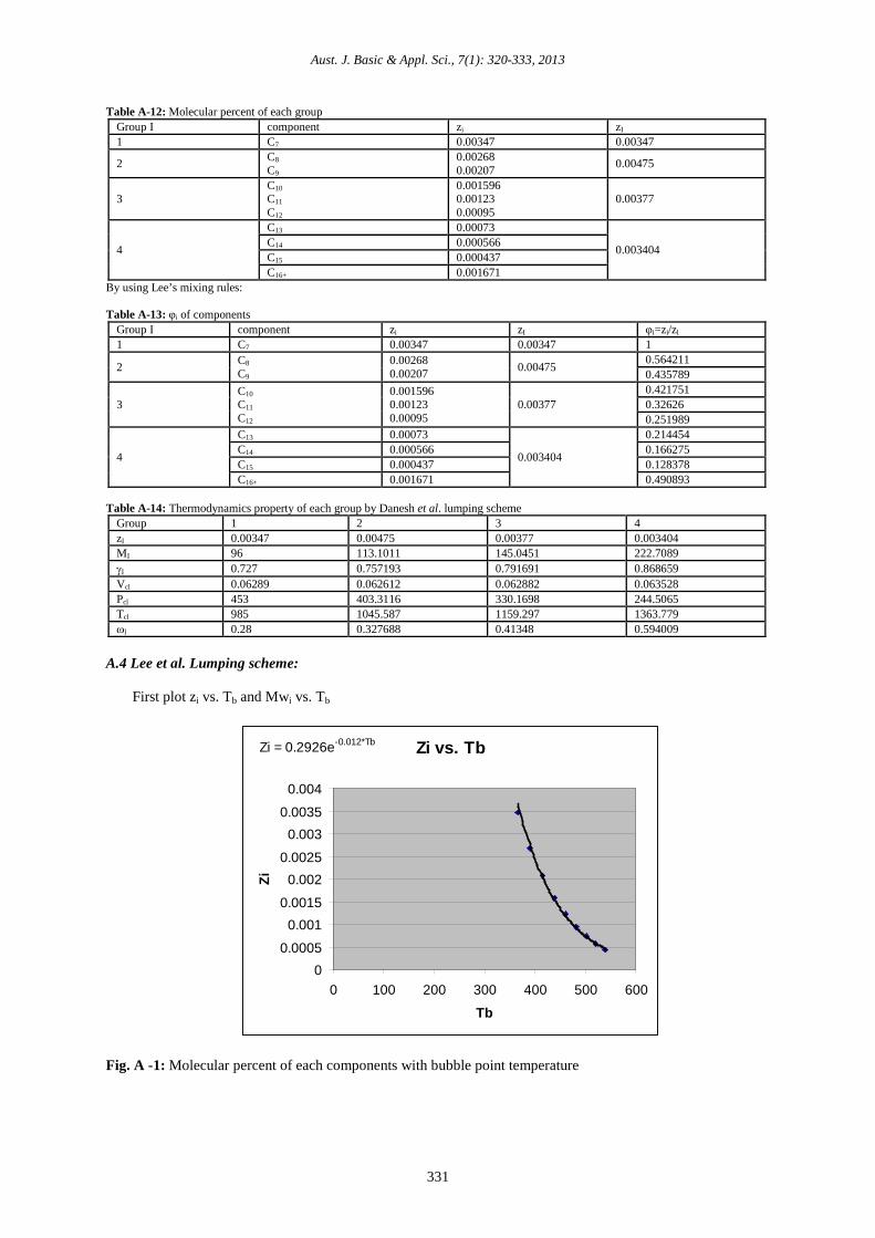
A.4 Lee et al. Lumping scheme:

First plot zi vs. Tb and Mwi vs. Tb

Fig. A -1: Molecular percent of each components with bubble point temperature

Zi vs. TbZi = 0.2926e-0.012*Tb

00.0005

0.0010.0015

0.0020.0025

0.0030.0035

0.004

0 100 200 300 400 500 600

Tb

Zi


332

Fig. A -2: Molecular weight of components with bubble point temperature

Set property of zi number 1 and property of Mwi number 2

21

=iw

component z Mwi Tb m i1 m i2 1im−

2im−

Mi

C7 0.00347 96 366 -4.3454E-05 0.5224 1 0.69 0.845

C8 0.00268 107 390 -3.258E-05 0.5224 0.7498 0.69 0.7199

C9 0.00207 121 416 -2.3848E-05 0.2524 0.5488 0.69 0.6194

C10 0.00159 134 439 -1.8096E-05 0.2524 0.4164 0.69 0.5532

C11 0.00123 147 461 -1.3898E-05 0.7571 0.3198 1 0.6599

C12 0.00095 161 482 -1.0802E-05 0.7571 0.2486 1 0.6243

C13 0.00073 175 501 -8.5996E-06 0.7571 0.1979 1 0.599

C14 0.000566 190 520 -6.8463E-06 0.7571 0.1576 1 0.5788

C15 0.000437 206 539 -5.4505E-06 0.7571 0.1254 1 0.5627

Table A-15: Molecular percent of each group


1 C7 0.00347 0.00615 C8 0.00268

2

C9 0.00207

0.007573

C10 0.001596 C11 0.00123 C12 C13

0.00095 0.00073

C14 0.000566 C15 0.000437

3 C16+ 0.001671 0.001671 By using Lee’s mixing rules: Table A-16: φi of components

Group I component zi zI φi=zi/zl

1 C7 0.00347 0.00615 0.564228 C8 0.00268 0.435772

2

C9 0.00207

0.007573

0.273339 C10 0.001596 0.209956 C11 0.00123 0.162419 C12 C13

0.00095 0.00073

0.125446 0.096395

C14 0.000566 0.074739

Mwi vs. Tb

Mwi = 0.5224*Tb - 95.878

Mwi = 0.7571*Tb - 203.2

0

50

100

150

200

250

0 100 200 300 400 500 600

Tb

Mw

i


333

C15 0.000437 0.057705 3 C16+ 0.001671 0.001671 1

Table A-17: Thermodynamics property of components by Lee lumping scheme

Group 1 2 3 zI 0.00615 0.007573 0.001671 MI 100.7935 148.2374 259 γI 0.736566 0.794528 0.908 Vcl 0.062774 0.062897 0.0638 Pcl 438.1837 331.5179 215 Tcl 1007.2 1155.6 1467 ωl 0.293945 0.41792 0.68

A.5 Behras and Stanndler lumping scheme

Staring component C7 Mole fraction (xD) 0.0154 MW 141.25

Step 1: The parameters of the semi continuous distribution in this example are A = 7 - 1/2 = 6.5 B =16 + 1/2 =16.5. Step 2: determine the slope of the distribution

375.1014

)425.141(=

+=

−

nc

Then

−

×+−= −−

−

αα

α

α *5.12*5.6

*5.1265.6375.101ee

e

α = 0.0011 Step 3 - Find integration points and weights C = (16.5-6.5)*0.0011 = 0.011 Because C< 0.3 so with this method cannot lump this oil.

Impact of Lumping Techniques for Fluid Characterization in...

Documents

Transcript of Impact of Lumping Techniques for Fluid Characterization in...