Impact of Brand Familiarity on Online and Offline Media ... of... · The Impact of Brand...

The Impact of Brand Familiarity on Online and Offli ne Media Synergy

ABSTRACT

Rooted in the Integrated Marketing Communication framework, this paper conceptualizes

how brand familiarity affects online and cross-channel synergies. The empirical analysis

uses Bayesian Vector Autoregressive models to estimate long-term elasticities for four

brands. The authors distinguish customer-initiated communication (typically online) from

firm-initiated communication (typically offline). Their results indicate that within-online

synergy is higher than online-offline synergy for both familiar brands but not for both

unfamiliar brands. Managers of unfamiliar brands may obtain substantial synergy from

offline marketing spending, even though its direct elasticity pales in comparison with that

of online media while managers of familiar brands can generate more synergy by

investing in different online media.

Keywords: marketing effectiveness, online paid, owned and earned media, synergy, integrated marketing communications, brand familiarity, Bayesian Vector Autoregression.

1

“Getting paid, owned and earned media to work in tandem, enhancing the effect of each is the ultimate goal,” Alistair Green, head of strategy, Mindshare (2012).

“You cannot build a brand simply on the Internet. You have to go offline,” J.G. Sandom Chairman and CEO at Mnemania (Pfeiffer and Zinnbauer 2010).

Since the introduction of the first banner ad in 1994, online advertising has

redefined the global advertising landscape. Spending in the sector has continued to grow,

reaching $117.60 billion globally in 2013 with expectations for this to reach $132.62

billion in 2014 and $173.12 billion by 2017 (EMarketer 2013). A key reason for this

popularity is that companies typically only pay for online media when prospective

customers take action, for example, by clicking on the ad or visiting the site (Bowman

and Narayandas 2001). In contrast to offline advertising spending, the long-term

effectiveness of online media is not well understood (Hanssens 2009). While Li and

Kannan (2014) found a low value of paid search response for a well-known hospitality

brand, they acknowledge that this result may be driven by the strength of the one brand

under study and call for future research. Insights on online media effectiveness are

important to Chief Marketing Officers, who are keenly interested in its return on

investment (CMO Survey 2013). Beyond the individual effectiveness of online media,

their synergy within-online and with offline media has only recently started to attract

academic scrutiny (Dinner, van Heerde and Neslin 2014; Naik and Peters 2009). Which

media types are most complementary with each other and thus produce synergy1 for

different brands?

We address this research question by assessing whether and how within-online

synergy and cross-channel synergy vary across brands. Building on research regarding 1 Throughout the paper, ‘synergy’ is bidirectional, as it arises when the combined effect or impact of a number of media activities is greater than the sum of their individual effects on sales (Schultz, Block and Raman 2012).

2

the effectiveness of banner ads (e.g., Manchanda, Dube, Goh and Chintagunta 2006),

paid search (e.g., Wiesel, Pauwels and Arts 2011; Dinner, van Heerde and Neslin 2014),

and social media conversations (e.g., Godes and Mayzlin 2004; Moe and Trusov 2011;

Sonnier, McAlister and Rutz 2011). We offer three contributions.

First, we provide a conceptual framework and an empirical analysis of how brand

familiarity influences online and cross-channel media synergy. Second, we analyze long-

term online media elasticities and synergies and provide empirical insights into the

interplay between online and offline media in driving synergy. As hypothesized, for

relatively unknown brands, the synergy of online media with offline media (cross-

channel synergy) is higher than within-online synergy. Finally, we illustrate the

managerial implications by comparing optimal budget allocations in the presence and

absence of such synergy. For the unfamiliar search brand analyzed in a previously

published paper (Wiesel et al. 2011), we show a dramatic change in the optimal budget

allocation, with the recommended online/offline allocation moving from 91% / 9% to

45% / 55% after incorporating synergy.

The rest of the article is organized as follows. After a description of related work, we

develop a conceptual framework based on which we offer hypotheses on online media

synergy with each other and with offline media. In the research methodology section, we

propose our Bayesian VAR econometric approach. We then describe the data set and present

our key findings on synergy as well as sales effectiveness of online and offline media, and

offer managerial implications for marketing budget allocation optimization. We conclude

the paper with a summary and a discussion of implications for practitioners and academics.

3

RESEARCH CONTEXT AND CONCEPTUAL FRAMEWORK

This section provides an overview of the extant research on online versus offline media

and the role of synergy within and among these media. Building on this, we propose a

conceptual framework that characterizes conditions under which offline and online media

should be most complementary with each other and thus produce synergy.

Customer-Initiated (Online) Media versus Firm-Initiated (Offline) Media

Recent marketing literature distinguishes between customer-initiated (often online)

and firm-initiated (often offline) media. Customer-initiated media (hereafter ‘online media’

for ease of exposition) charge companies only when (potential) customers actively click on,

search for and/or engage in online conversations about the company’s offerings (Bowman

and Narayandas 2001; Gartner 2008; Hoffman and Fodor 2010; Wiesel et al. 2011).2 In

contrast, firm-initiated media (hereafter ‘offline media’ for ease of exposition) can be

increased by companies without specific customer action, e.g., by doubling the TV

broadcasting time. Online media spending has surpassed offline radio and magazine

spending (Danaher and Dagger 2013), widening the call for research on its effectiveness

from both marketing academics and practitioners.

While online media used to be classified as paid, owned and earned online media

(Corcoran 2009), these distinctions are increasingly blurry. Still, the classification offers a

useful starting point for describing different types of online media.

2 Data on the fixed costs of setting up and running a website and hiring online media experts (online media) or developing traditional marketing messages are not generally available. We indirectly capture such efforts reflected in the higher effectiveness of weekly spending on online media as is typical in previous work (Wiesel et al. 2011).

4

Paid online media include online banner ads, affiliate marketing and paid search.

Affiliate marketing (Gallaugher, Auger and Barnir 2001) involves paying affiliates (e.g.,

Amazon) a percentage of the sales revenue generated when a customer is redirected from

the website of the affiliate to that of the company (e.g., Sony). Hoffman and Novak

(2000) find a low effectiveness of online banner ads, and propose affiliate marketing as a

more efficient way of customer acquisition. More recently, paid search has gained

popularity with US companies spending more than 40% of the total online advertising

dollars for paid search (Animesh, Ramachandran, and Viswanathan 2010). In paid search

(e.g., Google’s AdWords), advertisers bid for a position close to the top in the listing of

the paid search results which are displayed prominently on the top or side of organic

search results. Two recent studies find little, if any, incremental sales impact from paid

search for the studied brand, as verified in a field experiment of shutting off paid search

(Blake et al. 2015; Li and Kannan 2014).

Owned media includes the online media assets owned by a company, such as its

websites and their search engine optimization qualities, as reflected in organic search

results. Prospective customers visit a brand’s website to obtain more information

regarding the attractiveness of the product or service vis-à-vis competing offers (Li and

Kannan 2014). The strength of owned media is reflected in the company’s ranking in

organic search (Yang and Ghose 2010) and in the amount of ‘direct visits’, i.e. visitors

that type the company’s name directly into the URL (Li and Kannan 2014). Such ‘type-

in’ traffic may include loyal, repeat customers, and late-stage buyers who may have

already visited the site but needed time to make the purchase decision (Bustos 2008).

5

Earned media arises organically from consumers (Lieb and Owyang 2012). This

includes social media about the brand which includes blogging, microblogging (e.g.

Twitter), co-creation, social bookmarking, forums and discussion boards, product

reviews, social networks (e.g. Facebook) and video- and photo-sharing (Hoffman and

Fodor 2010). Consumers participate in these activities due to their desire to connect,

create, control and consume content (ibid). However, earned media are increasingly

‘fertilized’ by company employees (Trusov et al. 2009), with the blurred lines of, for

example, sharing sponsored content and native advertising (Wegert 2015). Foresee

Results (2011) reports high purchase conversion rates for visitors generated by social

media. However, social media has drawn criticism given the lack of consistent evidence

on sales results. For example, both Burger King and Pepsi reported poor sales

performance from their social media campaigns despite scoring well in terms of traffic

and customer engagement (Baskin 2011).

While the effectiveness of these separate online marketing actions has seen much

recent research attention, their synergy with each other, i.e. within-online synergy and

with offline media, i.e. cross-channel synergy, remains an important unresolved puzzle.

Synergy in Online Media and Offline Media

Synergy in media arises when the combined effect or impact of a number of

media activities is greater than the sum of their individual effects on sales (Schultz, Block

and Raman 2012). Social psychologists propose that the greater the number of sources

perceived to advocate a position, the higher is the perceived credibility (Cacioppo and

Petty 1979) and hence purchase intention (MacInnis and Jaworski 1989). Synergy has

been demonstrated within offline media (e.g. Edell and Keller 1989; Raman and Naik

6

2004), across offline and online media (e.g. Chang and Thorson 2004; Naik and Peters

2009; Reimer, Rutz and Pauwels 2014) and within online media (e.g. Schultz, Block and

Raman 2012; Kireyev, Gupta and Pauwels 2013; Li and Kannan 2014). However,

virtually all these studies analyze a single company, and do not examine to what extent

synergies differ for familiar versus unfamiliar brands. The presence of within-online

synergy implies a stronger allocation towards online media actions, while cross-channel

synergy implies a stronger role for offline marketing communication, which typically has

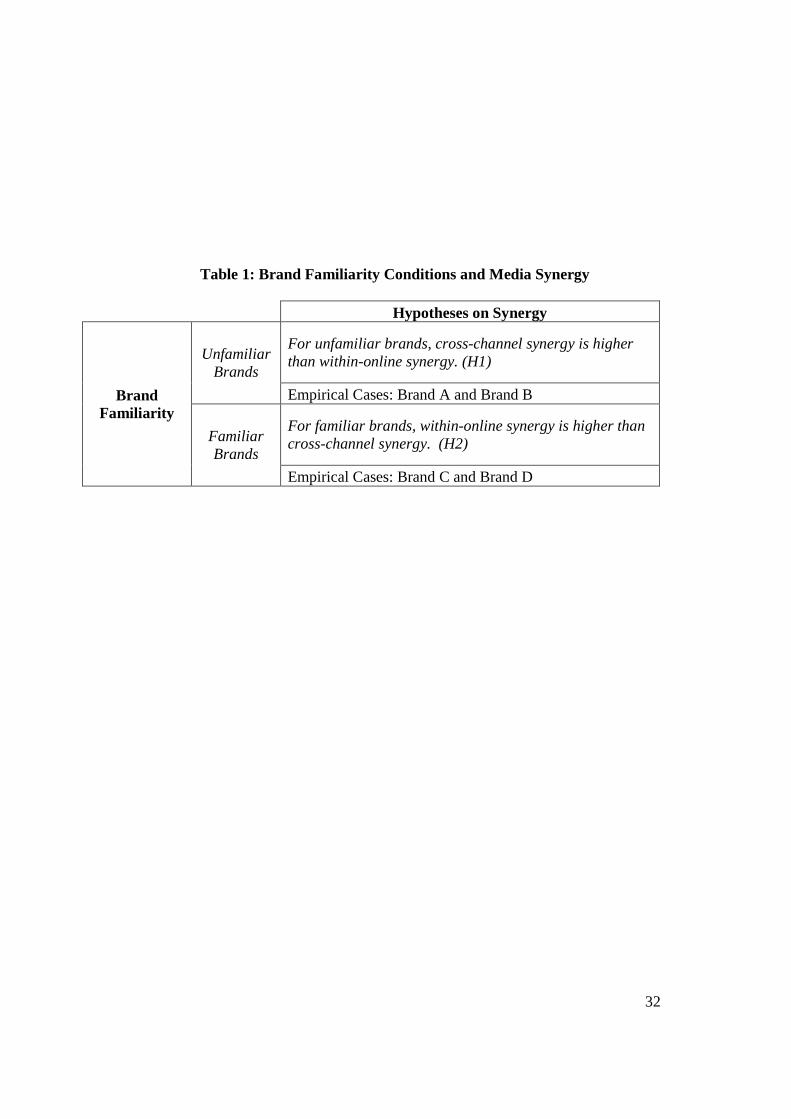
lower sales elasticity by itself (Wiesel et al. 2011). Our key thesis is that synergy should

differ for brands with high versus low familiarity among prospective customers, as

summarized in table 1. Brand familiarity captures consumers’ brand knowledge and

brand associations that exist within a consumer’s memory, representing one of the

components of customer-level brand equity (Keller and Lehmann 2006).3

---- Insert Table 1 around here ----

Selective attention theory (Kahneman 1973) implies that the use of multiple

media with repetition of ads lead to increased attention and elaboration. Attention is

highest for stimuli that are either both complex and familiar or are both simple and novel,

as compared to other combinations. Thus, if the stimulus is complex, the message needs

to be repeated in more media to increase familiarity. For less familiar brands, selective

attention theory implies managers should use multiple tools and invest in integrated

marketing communications (Stammerjohan et al. 2005). Unfamiliar brands still have to

build brand equity; they do not have the luxury to simply leverage existing brand equity

3 Brand equity also has other components (Keller 1993) but distinguishing these components is beyond the scope of this paper.

7

online (Pfeiffer and Zinnbauer 2010). Indeed, Ilfeld and Winer (2002) suggest that offline

firm-initiated communication will drive website traffic by increasing consumer

awareness. Additionally, high spending on both online and offline media may signal a

brand’s quality and create credibility. Other studies on unfamiliar brands showed that the

combination of offline and online advertising is more effective than repeated exposures in

either medium (Chang and Thorson 2004; Dijkstra, Buijtels and Van Raaij 2005).

Therefore, we propose that:

H1: For unfamiliar brands, cross-channel synergy is higher than within-online synergy.

In contrast, familiar brands run the risk of boring consumers (Anand and Sternthal

1990; Campbell and Keller 2003) and obtain little synergy among offline media actions

(Stammerjohan et al. 2005). Instead, familiar brands achieve higher click-through on their

online paid ads and more organic visits to their website (e.g. Yang and Ghose 2010; Ilfeld

and Winer 2002), thanks to their salient, rich and positive associations in consumers’

minds (Keller 1993). For instance, Vanguard was surprised to learn that most clicks on its

banner ads came from existing customers (McGovern and Quelch 2007). Such paid

exposure makes the existing link with the familiar brand more salient, and drives

consumers to the brand’s owned media. Therefore, we propose that:

H2: For familiar brands, within-online synergy is higher than cross-channel synergy.

We investigate these hypotheses for unfamiliar and familiar brands for brands in

four different categories, to help understand the generalizability of the recent findings in

the literature.

8

RESEARCH METHODOLOGY

Bayesian Vector Autoregressive Models

Our objectives and conceptual framework impose specific modeling requirements

that we outline here. First, we require a model that simultaneously incorporates several

online and offline marketing variables in addition to brand performance. Second, we need

to link the marketing variables to brand performance both directly and indirectly through

each other. In addition, the model needs to control for the effects of other marketing

actions such as feature and display as well as seasonality to avoid omitted variable bias.

Third, as the online and offline actions can influence each other over time, we need a

model that will accommodate these dynamic dependencies. Fourth, we need to obtain

immediate and cumulative effects of marketing variables on brand performance. Such

requirements have led many previous researchers to specify a Vector Autoregression

(VAR) model (e.g. Trusov et al. 2009, Wiesel et al. 2011). These models explicitly deal

with likely endogeneity (e.g., TV campaigns increase website visits, which increase sales)

by modeling each variable endogenously, i.e. explained by the dynamic system.

Unrestricted estimation of VAR models risks over-parametrization because the

parameter space proliferates with the number of endogenous variables, which include in

our case brand performance and several forms of online media and offline marketing.4 In

a standard VAR model, a large number of parameters may produce a good model fit, but

still result in multicollinearity and loss of degrees of freedom, which in turn may lead to

4 In our empirical application, the total number of parameters estimated for brand A, B, C and D is 198, 280, 280, and 264 respectively. Since this is infeasible with standard VAR approach, we use Bayesian VAR modeling, which imposes stochastic constraints on the parameters of the VAR model.

9

inefficient estimates and poor performance in the impulse-response functions. Bayesian

models alleviate such issues thanks to shrinkage, which imposes restrictions on the

parameters of the VAR model. We therefore outline a Bayesian VAR model (Sims and

Zha 1998; Horvath and Fok 2013) specification that meets our requirements.

Bayesian Vector Autoregressive (BVAR) models are formulated in Litterman (1986)

and Doan, Litterman and Sims (1984), but have seen little application in marketing (for an

exception see Horvarth and Fok 2013). Several priors have been used in the econometrics

literature to estimate the Bayesian VAR models, including Minnesota prior and Normal-

Wishart prior (e.g., Banbura, Giannone and Reichlin 2010; Ciccarelli and Rebucci 2003;

Kadiyala and Karlsson 1997; Sims and Zha 1998). Recently, Banbura, Giannone and

Reichlin (2010), using more than 100 variables, showed that the Minnesota prior leads to

improved forecasting performance compared to factor models. In general, the Minnesota

prior, which assumes a multivariate normal distribution, is superior to the Normal-Wishart

prior5 (Koop and Korobolis 2009). Using Doan et al.’s (1984) formula for the uncertainty of

the Minnesota prior means, we can specify individual prior variances for a large number of

coefficients in the model using only a few parameters (LeSage 1999). These parameters�, �

and w(i,j) represent the overall tightness, lag decay and the weighting matrix respectively.

We estimate the BVAR model through the “mixed estimation” technique developed by

Theil and Goldberger (1961). This method involves supplementing data with prior

information on the distributions of the coefficients (Ramos 2003). A typical unrestricted

VAR with n endogenous variables and p lags can be written as:

5 First, it greatly reduces the computational burden because it does not require MCMC methods. Rather, it leads to simple analytical results for the posterior and there is no need to use computationally demanding posterior simulation algorithms such as the Gibbs sampler. Second, it enables a wide flexibility when determining the prior.

10

�� = �� ,�� +⋯+��,�� + ��

� (1) Focusing on a single equation of the model:

� = �� + �(2) where y is the vector of observations on ��, the matrix X represent the lagged values of

�� , � = 1,… , � and the deterministic components, the vector A stands for the

coefficients of the lagged variables and deterministic components and � is the residual

vector. Prior restrictions for this single equation model can be written as:

�� ⋮��" = #$/$0⋮0 0$/$ ⋮0 ⋯⋯⋱⋯00⋮$/$��( �

⋮��" + �)) ⋮)��"(3) Here ��+� is the prior mean and $�+� is the standard deviation of the Minnesota prior

imposed on variable j in equation i at lag k, and ),()) = $ -. The standard deviation

defined by the Minnesota prior is as follows:

$�+� = . /�01 �2� = 3/.5�01 ∗ 789:;89<;= �2� ≠ 3 (4)

where � represents the tightness of the prior. It shows the standard deviation of the prior

on the first lag of the dependent variable. A higher tightness implies that less influence of

the lagged dependent variable in each equation. The parameter � stands for the decay

parameter taking the value between 0 and 1. The decay parameter reflects the fact that

standard deviation of the prior decreases as the lag length of the model increases. This

implies that further lags have less importance in the model. The parameter ? specifies the

relative tightness for variables other than the dependent variables. The parameter $+@ is

11

the standard error of the residuals obtained from the estimation of unrestricted single-

equation autoregression on variable j. The ratio of the standard errors in Eq. (4) is called a

scaling factor and accounts for the differences in the magnitudes of the variables across

equations i and j.

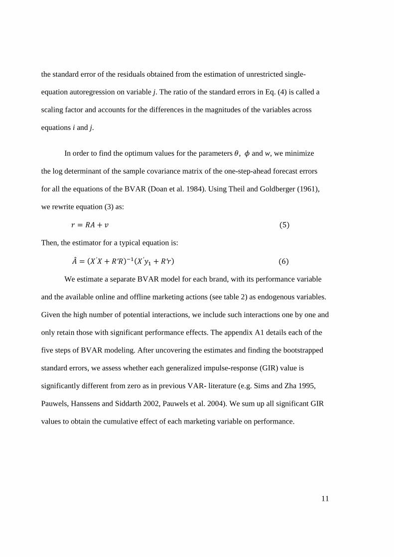
In order to find the optimum values for the parameters�, � and w, we minimize

the log determinant of the sample covariance matrix of the one-step-ahead forecast errors

for all the equations of the BVAR (Doan et al. 1984). Using Theil and Goldberger (1961),

we rewrite equation (3) as:

, = A� + )(5) Then, the estimator for a typical equation is:

�C = (�′� + A′A)�(�′� + A′,)(6) We estimate a separate BVAR model for each brand, with its performance variable

and the available online and offline marketing actions (see table 2) as endogenous variables.

Given the high number of potential interactions, we include such interactions one by one and

only retain those with significant performance effects. The appendix A1 details each of the

five steps of BVAR modeling. After uncovering the estimates and finding the bootstrapped

standard errors, we assess whether each generalized impulse-response (GIR) value is

significantly different from zero as in previous VAR- literature (e.g. Sims and Zha 1995,

Pauwels, Hanssens and Siddarth 2002, Pauwels et al. 2004). We sum up all significant GIR

values to obtain the cumulative effect of each marketing variable on performance.

12

DATA AND OPERATIONALIZATION

Assessing our hypotheses on long-term marketing elasticities and synergies

requires time-series data with at least 50 weekly observations (see Hanssens et al. 2001)

of brand performance and several online and offline media types. We were able to obtain

such data for brands from four companies across a variety of settings that substantially

differ on the relevant dimension of brand familiarity.

Brand A was launched less than 5 years before the data period, in the market for

scholastic test preparation. Using adaptive learning software, this company provides

flexible individual-level customization for scholastic test preparation. The absence of

fixed overhead costs due to no brick-and-mortar presence enables the company to price

competitively in the market. However, its business model represents a departure from the

traditional face-to-face interaction prevalent in this category. To communicate this

positioning, Brand A therefore uses a variety of online marketing efforts such as display

ads and paid search. During the global recession, the company communicated to

prospective customers that it would vary its price with stock market indices. Such

communicated price changes are the main firm-initiated actions by brand A.

Brand B is a family-run office furniture supplier without retail stores, they market

furniture directly to offices, hospitals, schools and individuals. Firm-initiated marketing

actions constitute the major part of its marketing budget and include direct mail and faxes

sent directly to prospective customers. Online marketing actions include email and paid

search. Brand B focuses on its product quality and delivery to the customer, assembly of

furniture, and customized furniture solutions.

13

Brand C is a top-five travel brand (Harris Interactive 2012). It provides travel-

related services to its customers for flights, hotels and cars. The company initiated its

marketing efforts with online communication but soon switched the budget to mostly

offline communication, including global television advertising campaigns. Marketing

communication actions include paid search, display, partner site links, television and out-

of-home advertising.

Brand D is a US apparel retail brand that was in the top 30 of Interbrand Best

Retail Brands 2013. Brand D’s products are targeted at the mass market with a focus on

casual apparel for men and women. The brand’s advertising is prominent and extensive,

and is present on multiple channels such as television, radio, print, and online paid

search. Store traffic is the main performance indicator for this retailer.

To verify third-party brand familiarity judgments, we assessed unaided and aided

brand awareness via survey respondents on Amazon’s Mechanical Turk.6 Our first four

survey questions (one per category) asked respondents to name three brands in the

category (unaided awareness). The next four questions inserted the studied brand name

and logo in random order among two known brands in the category, and asked

respondents which brands they recognized (aided awareness). The results reveal that

nobody spontaneously mentioned the scholastic test preparation service brand A as well

as office furniture brand B. In contrast, the travel website service brand C was mentioned

by 18 respondents (11%) as their first answer, by 21 (13%) as the second answer and by 6 Mturk is an online crowdsourcing system for recruiting survey respondents. Buhrmester, Kwang and Gosling (2011) showed that Mturk enables researchers to obtain high-quality data inexpensively and rapidly. The authors note that participants are more diverse than standard Internet or student samples and the data obtained is at least as reliable as the data obtained by traditional methods. Our survey was open for two weeks during May 2014, resulting in a total of 166 respondents and 160 usable answers.

14

22 (14%) as the third answer. Apparel retail brand D was mentioned by 7 (4.4%)

respondents as their first answer, by 16 (10%) as their second answer and by 10 (6.3%)

respondents as their third answer. As for aided awareness, 3% of respondents recognized

brand A, 3% recognized brand B, 76% recognized brand C and 96% recognized brand D.

Thus, our survey sample shows unaided (aided) awareness of 0% (3%) for both brands A

and B, 38% (76%) for brand C and 21% (96%) for brand D. Using these survey results as

well as the absence versus presence of the brands on the top-brands lists of Harris Poll

Equitrend Study and Interbrand, we conclude that brands A and B are relatively

unfamiliar, while brands C and D are relatively familiar to consumers.

All datasets are at the weekly level for a recent period of over a year. Brand A’s

data spans 2008 (week 40) to 2010 (week 8), with a total of 73 observations. Brand B’s

data spans 2007 (week 1) to 2010 (week 35), with 191 observations. Brand C’s data spans

2008 (week 1) to 2010 (week 35), with a total of 139 observations. Finally, Brand D’s

data spans 2010 (week 25) to 2011 (week 28), with 55 observations.

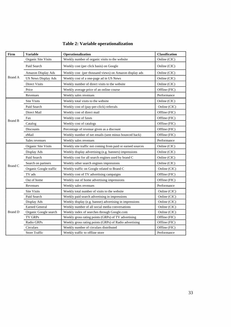
Data from all companies include the variables on online (customer-initiated)

media such as site visits and paid search, offline (firm-initiated) media and a performance

variable. Table 2 displays the variable operationalization.

--- Insert Table 2 about here ---

Our classification of each marketing action into customer-initiated (online) and firm-

initiated (offline) follows the definitions in our conceptual framework. Note that email is

a firm-initiated marketing action, because companies can increase spending on emails

without any prospective customer action. In contrast, our studied brands only pay for

15

display ads when a prospective customer clicks on them. Some online media are identical

among firms (e.g., paid search cost) while others are not (e.g., total website visits versus

only organic website visits). Likewise, the offline marketing actions differ by firm. This

is typical when moving from single-firm to multi-firm evidence; to the best of our

knowledge there is not yet a standardized dataset for online media (as e.g., the scanner

panel data for price, feature and display). To control for seasonality, we include four-

weekly seasonal dummies for brands A-C, using January as our benchmark. For brand D,

we use the national retail mall index, which offers weekly tracking of overall U.S. retail

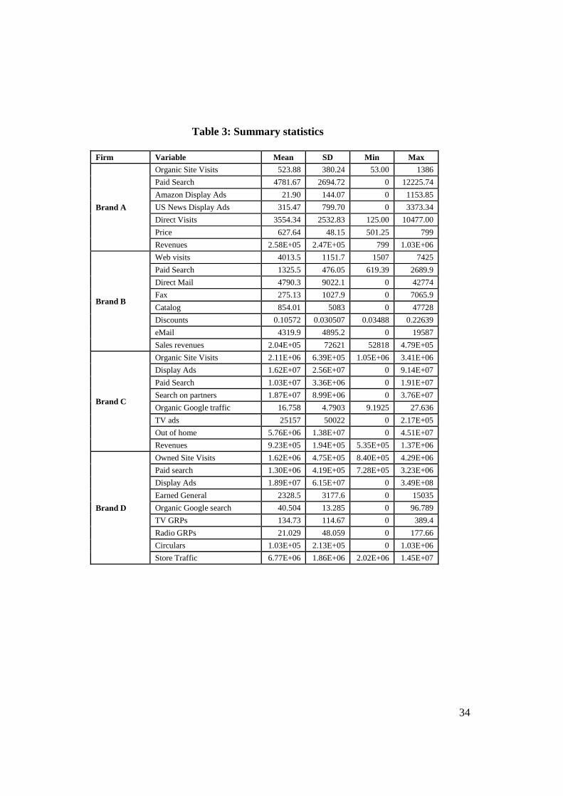
mall sales. As can be seen in Table 3, weekly average sales revenues for unfamiliar

brands A and B are below $260,000. In contrast, weekly average sales revenues of the

familiar brands C and D are above $900,000. Table 3 shows summary statistics for the

variables included in the model.


In light of the differences across firms in the data (Table 3), the log-log specification

helps with obtaining elasticity estimates, facilitating comparisons across brands.

EMPIRICAL FINDINGS

For each analyzed brand, both the AIC and SIC information criteria point to the inclusion

of one lag in the log-log model. The estimated models perform well in terms of

explanatory power, explaining 78% to 91% (adjusted R2=76% to 90%) of the variation in

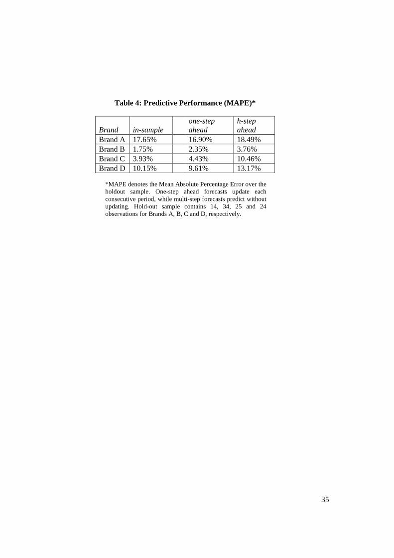
the performance variables. As to out-of-sample forecasting, we set aside the last 20% of

each brand’s time series to calculate the Mean Average Percentage Error (MAPE) for the

16

1-step ahead and the h-step ahead forecasts (with h the maximum number of hold-out

weeks).


While forecast errors are, as expected, larger for forecasts further in the future, the

highest MAPE remains below 18.5%, which indicates the high explanatory power of our

models is not due to overfitting. Moreover, the models show no violation of the

autocorrelation, heteroscedasticity, and normality assumptions for the residuals (Franses

2005), nor indicate omitted variable bias (Stock and Watson, 2003)7.We next discuss the

long-term elasticity estimates of marketing actions in the main-effects only models,

followed by an assessment of synergy, as a test of our proposed hypotheses.

Long-term elasticity of marketing actions (main effects models)

From the GIRFs, we obtain the total (cumulative) elasticity of each marketing action on

brand performance, as shown in Table 5 for the main effects BVAR model.


For each brand, the cumulative elasticity results show a substantially higher

performance impact for online customer-initiated media than for offline firm-initiated

media, consistent with previous literature (e.g. De Haan, Wiesel and Pauwels 2013;

Dinner, van Heerde and Neslin 2014; Wiesel, Pauwels and Arts 2011). Within online,

each brand shows the highest elasticity for prospective consumers coming to the owned

site (i.e. owned media): direct and organic site visits for brand A, site visits for brand B, 7 Ramsey RESET test tests the null hypothesis that the model has no omitted variable bias. The test results, available upon request, fail to reject that null hypothesis.

17

organic Google traffic and organic site visits for brand C, and organic Google search for

brand D. Among paid media, each brand shows the highest elasticity is for paid search.

To verify the robustness of our results, we also estimate the equivalent main effects

single-equation OLS model.8 Table 5 also shows the results, which are similar to the

BVAR findings in both sign and significance of the main effects. These results are as

expected since the main effects model has a relatively low number of parameters,

enabling OLS to be rather efficient.

What do these cumulative elasticities imply for marketing budget allocation? In

the absence of synergy, companies would be advised to spend a larger portion of the

communication budget on online media which have a larger elasticity than offline media

(Naik and Raman 2003). This is reflected in company practice of setting upper limits to

online advertising bids by multiplying the short-term conversion probability with margin

earned per conversion (Dinner et al. 2014). However, this does not account for either

long-term effects or synergy. Patterns in these effects allow us to assess our hypotheses

on within-channel versus cross-channel synergy.

Assessment of Synergy in Online and Offline Media

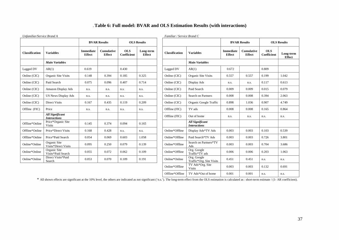
When we add interaction effects to our models, the results change as shown in table 6.

----- Insert Table 6 around here ----

From the BVAR results, we observe that synergy is present for each brand, as

several of the interactions are significant and often substantial compared to the main

8 To avoid multicollinearity, we log centered the variables in the OLS estimation..

18

effects. The single-equation OLS results show a similar pattern. For brands A and C, the

sign and significance of the parameters are the same. However, the OLS results show less

significant interaction terms for brands B and D, which is likely due to the high number

of parameters. We infer that OLS estimation is less efficient because it does not impose

any stochastic constraints on the estimated parameters as opposed to the BVAR model.

In testing our hypotheses, we compare the within-channel versus cross-channel

synergy effects in two ways. First, we consider the synergy with the median effect (across

all actions for that synergy type) and the synergy with the highest estimated effect for that

synergy type (hereafter ‘best in breed’). This allows us to assess the hypotheses on both

of these benchmarks. Specifically, based on the GIRF estimates, for each brand we

conduct a two- tailed t-test to test our hypotheses for (i) the ‘typical’ (median elasticity)

action for each synergy type, and (ii) the best-in-breed (highest elasticity) action for each

synergy type.

Table 7 provides these results. The panel on the left corresponds to the tests for the typical

synergy while the panel on the right corresponds to the test for the best-in-breed synergy.

Within each panel, the synergy type (within-online and cross-channel), and the

corresponding median or maximum are listed in the first and second columns, respectively.

The hypothesis tested is in the third column while the final column in each panel gives the

outcome of the t-test. For example, unfamiliar brand A experiences an elasticity of 0.374 for

median (‘typical’) cross-channel synergy and 0.428 for maximum (best-in-breed) cross-

channel synergy. These numbers come from the cumulative effect of price*organic visits

(0.374 in table 7) and price*direct visits (0.428 in table 7), with price*paid search (0.069 in

table 7) is the lowest elasticity for cross-channel synergy.

19


We first report the median (‘typical’ action) results. We compare the cross

synergy between online and offline media with the within-online synergy, focusing on the

unfamiliar brands A and B. As seen from Table 5, cross synergy is higher than within-

online synergy for both unfamiliar brands A and B (0.374 vs. 0.072 with p <.1 and 0.044

vs. 0.004 with p >.1, respectively). Based on the best-in-breed results, the same finding

holds, i.e. cross synergy is higher than within-online synergy (0.428 vs. 0.250 with p > .1

for brand A and 0.554 vs. 0.004 with p <.01 for brand B).

For familiar brands for the typical action results, within-online synergy is higher

than cross-synergy for both brands C and D (0.451 vs. 0.003 with p <.01 and 0.213 vs.

0.003 with p <.01, respectively). The same finding holds for the ‘best-in-breed’ results

(0.451 vs 0.006 with p <.01 for brand C and 0.336 vs. 0.004 with p <.01 for brand D).

Implications

Our framework and empirical results shed light on a number of important implications in

understanding the potential benefits of synergy in different online advertising media. The

results show that ‘within online synergy’ is significantly higher than ‘cross channel synergy’

for familiar brands in our data, which may mean that, high and favorable awareness has

already been created in offline media for well-known brands. An alternative explanation

may be that familiar brands are more likely to spend near-optimally while unfamiliar brands

spend far below optimal, which leads to higher returns from increasing spending.9 However,

this would not explain why familiar brands have higher within-online synergy. Moreover,

9 We thank the Associate Editor and an anonymous reviewer to bring this to our attention.

20

this explanation would require systematic differences in spending effectiveness for familiar

versus unfamiliar brands – which we do not observe in the results tables.

We also find that owned media has a higher sales elasticity than paid media for

unfamiliar brands and for the familiar service brand. Thus, owned media is a credible

source for consumers to decrease the unpredictable nature of services and of unfamiliar

brands. By contrast, we find that sales elasticity of paid media is higher than owned

media for familiar product brand. In the latter instance, paid media can provide enough

information with which to evaluate the quality and enables the firm to maximize reach for

familiar products.

Finally, how do our results relate to the recent findings that (certain types of) paid

media are not effective in lifting sales for a well-known hospitality brand (Li and Kannan

2014) but effective in lifting sales for a relatively unknown furniture brand (Wiesel et

al.2011)? First, the company studied in Li and Kannan (2014) is similar to our brand C,

and they too find a low sales impact for paid media and a large within-online ‘spillover’

(synergy). Our research implies that such findings do not generalize to unfamiliar brands,

thus confirming Li and Kannan’s (2014) speculation that unfamiliar brands face a

different marketing type effectiveness challenge. Second, while Wiesel et al. (2011) study

the same brand as our brand B and report a strong effect of paid search, they do not

incorporate synergy, and thus miss an important part of picture (Li and Kannan 2014).

We show this next by calculating optimal allocation recommendations with synergy

versus without synergy (i.e. the main effects model of table 5).

21

Marketing Budget Allocation Optimization

Our empirical estimation yields marketing spending elasticities that managers can

use to optimize their marketing budget allocation under the usual caveats that the model

specification captures the major drivers of sales and that the near future is similar to the past.

We illustrate the importance of synergy using this procedure, we present the allocation

optimization for unfamiliar brand B analyzed by Wiesel et al. (2011) in a model without

synergy.

From the log-log BVAR model, we derive the marketing-sales elasticities as the total

over-time impact captured by the Generalized Impulse Response Functions. For the main

effects model, each marketing action is allocated a budget corresponding to its elasticity

compared to the elasticity of the other marketing actions (Dorfman and Steiner 1954; Wright

2009). For the synergies model, the marginal elasticity of marketing action X1 depends on

the level of the other marketing action X2. Assuming the level of X2 is fixed at the mean

values of the variables, we combine the main effect and the interaction effect for X1’s

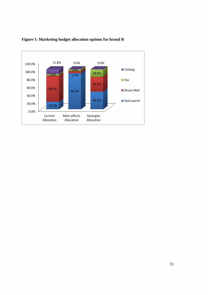
elasticity (Naik and Raman 2003, see appendix A2 for details). Figure 1 contrasts the current

allocation, the optimal allocation from the BVAR model without synergy, and the optimal

allocation from the BVAR model with synergies.

---- Insert Figure 1 about here ----

Due to the high relative elasticity of online paid search, the main effects BVAR model

implies that brand B should increase its paid search spending from 18% to 91% of its

budget, dropping its main marketing activity, direct mail, from 66% to 6%. Catalogs are

found to be ineffective, and thus should be set to 0% in the optimal allocation while fax

spending should remain at its current level. This reallocation is similar to the one implied in

22

Wiesel et al. (2011). However, the offline actions of direct mail and fax have strong

synergies with online search, and the allocation that accounts for these synergies (the right

column in Figure 1) suggests a more balanced budget. Online paid search receives 44.5%,

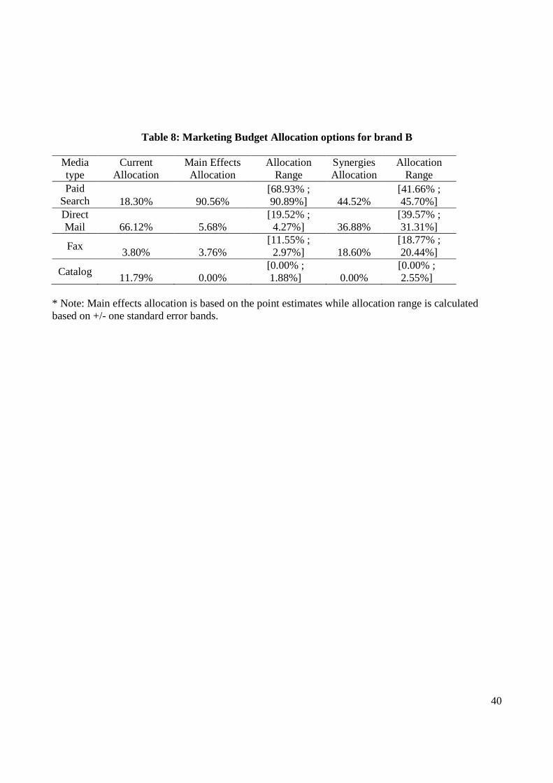
while direct mail receives 36.9% and fax 18.6%. We also calculate the confidence bounds to

account for the uncertainty in these allocations, as shown in Table 8.

---- Insert Table 8 about here ----

Overall, the findings suggest that online paid search and direct mail work synergistically in

conjunction with faxes in driving sales for brand B. Accounting for synergies among

marketing actions can thus lead to substantially different optimal marketing resource

allocation.

CONCLUSIONS, LIMITATIONS AND FUTURE RESEARCH

In this study, we provide a conceptual framework on cross-channel and infra-channel

synergies by taking into consideration brand familiarity. We propose that unfamiliar

brands have to build brand equity in multiple channels, and cannot simply leverage

existing brand equity online. For unfamiliar brands, the combination of offline and online

marketing (cross-synergy) matters more than intra-channel synergy. Familiar brands, on

the other hand, are better able to leverage their brand equity online since consumer

knowledge is already high to begin with.

We illustrate the framework’s applicability for two familiar and two unfamiliar

brands. The empirical results obtained from BVAR estimations showed that within-online

synergy is significantly higher than cross-channel synergy for the studied familiar brands,

while unfamiliar brands experience higher synergy of online media with offline

23

marketing, which implies they should spend more on offline media than implied by their

low direct sales elasticity. This paper is the first to show cross-channel synergies of

online media with direct mail (brand B) and with radio (brand D). Consistent with

previous results, we also find synergy among TV and online media for every analyzed

brand that invested in TV ads (Chang and Thorson 2004). As developed in Raman and

Naik (2004), synergy effects imply that any medium deserves a non-zero budget despite

its limited or unknown effectiveness. The high within-online synergy for familiar brands

also provides a boundary condition for the advice that “Once a brand is familiar;

expenses can be curtailed by reducing the number and types of media” (Stammerjohan et

al. 2005; p.65).

Our results have important implications for marketing theory. First of all, our

results add to online media research by addressing how effectiveness varies with brand

familiarity. Second, although research on synergy is growing, the conditions for synergy

(just as brand-related effects and the use of social media) are still mostly neglected. Our

study demonstrates the importance of incorporating brand familiarity into models for

integrated marketing communications (Winer 2009). Furthermore, it addresses the need

for new methods and approaches going beyond offline media forms by incorporating new

developments on online media.

Our work has also important implications for marketing practitioners. First,

managers of unfamiliar brands may obtain substantial synergy from offline marketing

spending, even though its direct elasticity pales in comparison with that of online media.

Second, our results show that managers of familiar brands can generate more synergy by

investing in different online media, thus confirming the opening quote by Green (2012).

24

Our study is not free of limitations. The use of data of two unknown and two

known brands limit the generalizability of our results. However, the aim of this study is to

obtain insights on the effectiveness of especially new advertising formats for different

conditions rather than offering empirical generalizations (EGs). Future research should

offer EGs on this topic. Additionally, the selection of variables is limited to their

availability in the data sets – omitted variables include the focal brand’s quality changes

and new product introductions, competitive communication spending and market

environment factors. Specifically relevant for the purpose of this paper, we had different

offline and online advertising types across brands. Future research should define metrics

that are most appropriate for earned, owned or paid media measurement. Defining and

proposing metrics for new advertising formats is an important need in the area. As typical

in budget allocation across media, we have assumed that the studied brands tactically

execute their communication in a similarly competent manner (and therefore that

substantially lower effectiveness of a medium is not simply due to its poor execution).

Future research may test this assumption. In addition, it would be useful to investigate

how our results on the impact of brand familiarity on media synergy vary over the

product life cycle. Furthermore, practitioners, data providers and academics should

collaborate to explore the possibility of standardized datasets for paid, owned, earned

media (as e.g., scanner panel data for price, feature and display), which represents both a

challenge and an opportunity. We also identify an opportunity for future research on the

methods used. In our BVAR modeling with a Minnesota prior, we assume that the off-

diagonal elements in the prior variance-covariance matrix are zero to simplify

25

computation. Future research can allow for more flexible variance-covariance matrix

using more complex estimations based on MCMC methods.

Another research area is to understand the differentiated effect of various online

advertising mediums along the different stages of consumer decision-making. The

interplay between different online advertising formats and effects of brand familiarity or

product-service dichotomy may vary through these different stages of consumer decision

making. Additionally, we show a greater sales elasticity for ‘within-online synergy’ for

familiar brands. However, the results are mixed for unfamiliar brands. This area may

need additional investigation.

In summary, our research is the first to conceptually and empirically investigate

how brand-familiarity impacts online media synergy as well as online and offline media

synergy. We believe this work puts recent single-firm findings into perspective and we

hope to inspire further research towards empirical generalizations on the effectiveness of

new and established media.

26

REFERENCES

Anand, Punam and Brian Sternthal (1990), “Ease of Message Processing as a Moderator of Repetition Effects in Advertising,” Journal of Marketing Research, 27 (August), 345–353.

Animesh, Animesh, Vandana Ramachandran, and Siva Viswanathan (2010), “Quality Uncertainty and the Performance of Online Sponsored Search Markets: An Empirical Investigation,” Information Systems Research, 21 (1), 190-201.

Banbura, Marta, Domenico Giannone, and Lucrezia Reichlin (2010), “Large Bayesian Vector Auto Regressions,” Journal of Applied Econometrics, 25, 71-92. Baskin, Jonathan S. (2011), “Do Campaign Failures, High-Profile Firings Signal the End of Social Media?,” (accessed March 22, 2011), [available at http://adage.com/article/cmo-strategy/pepsi-burger-king-news-signal-end-social-media/149523/].

Blake, Thomas, Chris Nosko, and Steven Tadelis (2013), “Consumer Heterogeneity and Paid Search Effectiveness: A Large Scale Field Experiment,” Econometrica, 83(1), 155-174.

Bowman, Douglas and Das Narayandas (2001), “Managing Customer-Initiated Contacts with Manufacturers: The Impact on Share of Category Requirements and Word-of-Mouth Behavior,” Journal of Marketing Research, 281-297.

Buhrmester, Michael, Tracy Kwang, and Samuel D. Gosling (2011). Amazon’s Mechanical Turk: A New Source of Inexpensive, Yet High-Quality, Data? Perspectives on Psychological Science, 6(1), 3-5. Bustos, Linda (2008), “The Forgotten Metric: Direct Traffic Reveals Brand Strength,” (accessed July 31, 2009), [available at http://www.getelastic.com/direct-traffic-google-analytics/].

Cacioppo, John T. and Richard E. Petty (1979), “Effects of Message Repetition and Position on Cognitive Response, Recall, and Persuasion,” Journal of Personality and Social Psychology, 37(1), 97.

Campbell, Margaret C. and Kevin Lane Keller (2003), “Brand Familiarity and Advertising Repetition Effects,” Journal of Consumer Research, 30(September), 292-304. Chang, Yuhmiin and Esther Thorson (2004), “Television and Web Advertising Synergies,” Journal of Advertising, 33 (2), 75-84.

Ciccarelli, Matteo and Alessandro Rebucci (2003), “Bayesian VARs: A Survey of the Recent Literature with an application to the European Monetary System,” Working Paper No. 03/102, International Monetary Fund. CMO Survey (2013), “CMOs on Social Media: Where’s the ROI?,” (accessed May 1, 2015) [at http://www.forbes.com/sites/dorieclark/2013/09/12/cmos-on-social-media-wheres-the-roi/].

Corcoran, Sean (2009), “Defining Earned, Owned and Paid Media,”, (accessed May 1, 2015), [available at http://blogs.forrester.com/interactive_marketing/2009/12/defining-earned-owned-and-paid-media.html].

27

Danaher, Peter J. and Tracey S. Dagger (2013), “Comparing the Relative Effectiveness of Advertising Channels: A case Study of a Multimedia Blitz Campaign,” Journal of Marketing, 50 (August), 517-534.

De Haan, Evert D., Thorsten Wiesel, and Koen Pauwels (2013), “Which Advertising Forms Make a Difference in Online Path to Purchase?” Working Paper Series No. 13, Marketing Science Institute.

Dijkstra, Majorie, Heidi E.J.J.M. Buijtels, and W. Fred Van Raaij (2005), “Separate and Joint Effects of Medium Type on Consumer Responses: A Comparison of Television, Print, and the Internet,” Journal of Business Research, 58, 377-386.

Dinner, Isaac. M., Harald J. Van Heerde, and Scott Neslin (2014), “Driving Online and Offline Sales: The Cross-channel Effects of Digital versus Traditional Advertising,” Journal of Marketing Research, 51 (5), 527-545

Doan, Thomas, Robert B. Litterman, and Christopher A. Sims (1984), “Forecasting and Conditional Projection Using Realistic Prior Distributions,” Econometric Reviews, 3, 1-100.

Dorfman, Robert and Peter O. Steiner (1954), “Optimal Advertising and Optimal Quality,” The American Economic Review, 44 (5), 826-836.

Edell, Julie A. and Kevin L. Keller (1989), “The Information Processing of Coordinated Media Campaigns,” Journal of Marketing Research, 26 (May), 149–63.

EMarketer (2013), “Worldwide Ad Growth Buoyed by Digital, Mobile Adoption,” (accessed July 21, 2013), [available at http://www.emarketer.com/Article/Worldwide-Ad-Growth-Buoyed-by-Digital-Mobile-Adoption/1010244].

Foresee Results (2011), “Social Media Marketing: Do Retail Results Justify Investment,” (accessed September 15th, 2014), [available at http://www.scribd.com/doc/204504338/Social-Media-Marketing-u-s-2011-Foresee.]

Franses, Philip H. (2005), “On the Use of Econometric Models for Policy Simulation in Marketing,” Journal of Marketing Research, 42(1), 1-14.

Gallaugher, John M., Pat Auger, and Anat Barnir (2001), “Revenue Streams and Digital Content Providers: An Empirical Investigation,” Information and Management, 38 (7), 473-485.

Gartner, Inc (2008), “A Checklist for Evaluating an Inbound and Outbound Multichannel Campaign Management Application,” (accessed September, 2010), [available at https://www.gartner.com/doc/750252/checklist-evaluating-inbound-outbound-multichannel]

Godes, David and Dina Mayzlin (2004), “Using Online Conversations to Study Word-of-Mouth Communication,” Marketing Science, 23(4), 545-560.

Green, Alistair (2012), “Paid, Owned and Earned Media: Integration’s Holy Grail,” (accessed September 13, 2014), [available at http://www.greatmediaminds.net/2012/05/31/paid-owned-and-earned-media-integrations-holy-grail/].

Hanssens, Dominique M. (2009), Empirical Generalizations about Marketing Impact: What We Have Learned from Academic Research. Cambridge: Marketing Science Institute.

28

———, Leonard J. Parsons, and Randall L. Schultz (2001), Market Response Models: Econometric and Time Series Analysis. 2nd Edition, Kluwer Academic Publishers.

Harris Interactive (2012),” (accessed September 16, 2014, 2014), [available at http://www.prnewswire.com/news-releases/top-ranked-travel-brands-southwest-kayak-royal-caribbean-and-enterprise-continue-to-rule-the-industry-as-brands-of-the-year-according-to-the-23rd-annual-harris-poll-equitrend-study-146794695.html].

Hoffman, Donna L. and Thomas P. Novak (2000), “How to Acquire Customers on the Web,” Harvard Business Review. May-June, 78 (3), 179-183.

——— and Marek Fodor (2010), “Can You Measure the ROI of Your Social Media Marketing?,” MIT Sloan Management Review, 52 (1), 41-49.

Horvath, Csilla and Dennis Fok (2013), “Moderating Factors of Immediate, Gross, and Net Cross-Brand Effects of Price Promotions,” Marketing Science, 32 (1), 127-152.

Ilfeld, Johanna S. and Russell S. Winer (2002), “Generating Website Traffic,” Journal of Advertising Research, 42 (5), 49-61.

Kadiyala, K. Rao and Sune Karlsson (1997) “Numerical Methods for Estimation and Inference in a Bayesian VAR-Models,” Journal of Applied Econometrics, 12, 99-132.

Kahneman, Daniel (1973), Attention and Effort. New Jersey: Prentice Hall, Englewood Cliffs.

Keller, Kevin L. (1993), “Conceptualizing, Measuring and Managing Customer-based Brand Equity,” Journal of Marketing, 57(1), 1-22.

Kireyev, Pavel, Koen Pauwels, and Sunil Gupta (2013), “Do Display Ads Influence Search? Attribution and Dynamics in Online Advertising,” Working Paper No. 13-070, Harvard Business School.

Koop, Gary and Dimitris Korobilis (2009), “Bayesian Multivariate Time Series Methods for Empirical Macroeconomics,” Foundations and Trends in Econometrics, 3 (4), 267-358.

LeSage, James P. (1999), “Applied Econometrics Using Matlab,” (accessed September 7, 2010), [available at http://www.spatial-econometrics.com/html/mbook.pdf].

LeSage, James P. and Anna Krivelova (1999), “A Spatial Prior for Bayesian Vector Autoregressive Models,” Journal of Regional Science, 39(2), 297-317.

Li, Hongshuang, and P. K. Kannan (2014),”Attributing Conversions in a Multichannel Online Marketing Environment: An Empirical Model and a Field Experiment,” Journal of Marketing Research 51 (1), 40-56.

Lieb, Rebecca and Jeremiah Owyang (2012), “The Converged Media Imperative: How Brands must combine Paid, Owned and Earned Media”, Altimeter Report, July 18, accessed December 13, 2014: http://www.slideshare.net/Altimeter/the-converged-media-imperative.

Litterman, Robert B. (1986), “Forecasting with Bayesian Vector Autoregressions: Five years of Eexperience,” Journal of Business and Economic Statistics, 4, 25-38.

29

MacInnis, Deborah J. and Bernard J. Jaworski (1989), “Information Processing from Advertisements: Toward an Integrative Framework,” Journal of Marketing, 53 (October), 1-23.

Manchanda, Puneet, Jean-Pierre Dube, Khim Y. Goh, and Pradeep K. Chintagunta (2006), “The Effect of Banner Advertising on Internet Purchasing,” Journal of Marketing Research, 43 (1), 98-108.

McGovern, Gail and John A. Quelch (2007), Measuring Marketing Performance. Harvard Business School Multimedia Tool.

Moe, Wendy W. and Michael Trusov (2011), “The Value of Social Dynamics in Online Product Ratings Forums, Journal of Marketing Research, 48(3) 444–456.

Naik, Prasad A. and Kay Peters (2009), “A Hierarchical Marketing Communications Model of Online and Offline Media Synergies,” Journal of Interactive Marketing, 23 (4), 288-299.

——— and Kalyan Raman (2003), “Understanding the Impact of Synergy in Multimedia Communications,” Journal of Marketing Research, 40 (4), 375-88.

Pauwels, Koen, Dominique M. Hanssens, and S. Siddarth (2002), “The Long-term Effects of Price Promotions on Category Incidence, Brand Choice, and Purchase Quantity,” Journal of Marketing Research, 39 (4), 421-439.

———, Jorge Silva-Risso, Shuba Srinivasan, and Dominique M. Hanssens (2004), “New Products, Sales Promotions, and Firm Value: The Case of the Automobile Industry. Journal of Marketing, 68 (October), 142-56.

Pesaran, H. Hashem and Yongcheol Shin (1998), “Generalized Impulse Response Analysis in Linear Multivariate Models,” Economic Letters, 58 (1), 17-29.

Pfeiffer, Markus and Markus Zinnbauer (2010), “Can Old Media Enhance New Media? How Traditional Advertising Pays off for an Online Social Network,” Journal of Advertising Research, 50(1), 42-49. Raman, Kalyan and Prasad A. Naik (2004), “Long-term Profit Impact of Integrated Marketing Communications Program,” Review of Marketing Science, 2 (1), 21-23.

Ramos, Riberio F. F. (2003), “Forecasts of Market Shares from VAR and BVAR Models: A Comparison of Their Accuracy,” International Journal of Forecasting, 19, 95-110. Reimer, Kerstin, Oliver J. Rutz, and Koen Pauwels (2014), “How Online Consumer Segments Differ in Long-term Marketing Effectiveness,” Journal of Interactive Marketing, 28(4), 271-284. Schultz, Don E., Martin P. Block, and Kaylan Raman (2012), “Understanding Consumer-created Media Synergy,” Journal of Marketing Communications, 18 (3), 173-187.

Sims, Christopher A., James H. Stock, and Mark W. Watson (1990), “Inference in Linear Time Series Models with Some Unit Roots,” Econometrica, 58 (1), 113-144. ——— and Tao Zha (1998), “Bayesian Methods for Dynamic Multivariate Models,” International Economic Review, 39 (4), 949-968.

30

Sonnier, Garrett P., Leigh McAlister and Oliver J. Rutz (2011), “A Dynamic Model of the Effect of Online Communications on Firm Sales,” Marketing Science, 30(4), 702-716.

Stammerjohan, Claire, Charles M. Wood, Yuhmiin Chang, and Esther Thorson (2005), “An Empirical Investigation of the Interaction between Publicity, Advertising, and Previous Brand Attitudes and Knowledge. Journal of Advertising, 34 (4), 55-67.

Stock James H. and Mark W. Watson (2003). Introduction to Econometrics. New York: Prentice Hall. Theil, Henri and Arthur S. Goldberger (1961), “On Pure and Mixed Statistical Estimation in Economics,” International Economic Review, 2, 65-78.

Trusov, Michael, Randolph E. Bucklin and Koen Pauwels (2009), “Effects of Word of Mouth versus Traditional Marketing: Findings for an Internet Social Networking Site,” Journal of Marketing, 73 (5), 90-102.

Wegert, Tessa (2015), “Why the New York Times’ sponsored content is going toe-to-toe with its editorial”, Contently, March 27, (accessed June 4th 2015), [available at http://contently.com/strategist/2015/03/27/why-the-new-york-times-sponsored-content-is-going-toe-to-toe-with-its-editorial/

Wiesel, Thorsten, Koen Pauwels, and Joep Arts (2011), “Marketing’s Profit Impact: Quantifying Online and Off-line Funnel Progression,” Marketing Science, 32, 229-245.

Winer, Russell S. (2009), “New Communications Approaches in Marketing: Issues and Research Directions,” Journal of Interactive Marketing, 23 (2), 108-117.

Wright, Malcolm (2009), “A New Theorem for Optimizing the Advertising Budget,” Journal of Advertising Research, 49 (2), 164-169.

Yang, Sha and Anindya Ghose (2010), “Analyzing the Relationship between Organic and Sponsored Search Advertising: Positive, Negative or zero interdependence?” Marketing Science, 29 (4), 602-623.

31

Figure 1: Marketing budget allocation options for brand B

0.0%

20.0%

40.0%

60.0%

80.0%

100.0%

120.0%

Current

Allocation

Main effects

Allocation

Synergies

Allocation

18.3%

90.6%

44.5%

66.1%

5.7%

36.9%

3.8%

3.8%18.6%

11.8% 0.0% 0.0%

Catalog

Fax

Direct Mail

Paid search

32

Table 1: Brand Familiarity Conditions and Media Synergy

Hypotheses on Synergy

Brand Familiarity

Unfamiliar Brands

For unfamiliar brands, cross-channel synergy is higher than within-online synergy. (H1)

Empirical Cases: Brand A and Brand B

Familiar Brands

For familiar brands, within-online synergy is higher than cross-channel synergy. (H2)

Empirical Cases: Brand C and Brand D

33

Table 2: Variable operationalization

Firm Variable Operationalization Classification

Brand A

Organic Site Visits Weekly number of organic visits to the website Online (CIC)

Paid Search Weekly cost (per click basis) on Google Online (CIC)

Amazon Display Ads Weekly cost (per thousand views) on Amazon display ads Online (CIC)

US News Display Ads Weekly cost of a one-page ad in US News Online (CIC)

Direct Visits Weekly number of direct visits to the website Online (CIC)

Price Weekly average price of an online course Offline (FIC)

Revenues Weekly sales revenues Performance

Brand B

Site Visits Weekly total visits to the website Online (CIC)

Paid Search Weekly cost of (pay-per-click) referrals Online (CIC)

Direct Mail Weekly cost of direct mail Offline (FIC)

Fax Weekly cost of faxes Offline (FIC)

Catalog Weekly cost of catalogs Offline (FIC)

Discounts Percentage of revenue given as a discount Offline (FIC)

eMail Weekly number of net emails (sent minus bounced back) Offline (FIC)

Sales revenues Weekly sales revenues Performance

Brand C

Organic Site Visits Weekly site traffic not coming from paid or earned sources Online (CIC)

Display Ads Weekly display advertising (e.g. banners) impressions Online (CIC)

Paid Search Weekly cost for all search engines used by brand C Online (CIC)

Search on partners Weekly other search engines impressions Online (CIC)

Organic Google traffic Weekly traffic on Google related to Brand C Online (CIC)

TV ads Weekly cost of TV advertising campaigns Offline (FIC)

Out of home Weekly out of home advertising impressions Offline (FIC)

Revenues Weekly sales revenues Performance

Brand D

Site Visits Weekly total number of visits to the website Online (CIC)

Paid Search Weekly paid search advertising in impressions Online (CIC)

Display Ads Weekly display (e.g. banner) advertising in impressions Online (CIC)

Earned General Weekly number of all social media conversations Online (CIC)

Organic Google search Weekly index of searches through Google.com Online (CIC)

TV GRPs Weekly gross rating points (GRPs) of TV advertising Offline (FIC)

Radio GRPs Weekly gross rating points (GRPs) of Radio advertising Offline (FIC)

Circulars Weekly number of circulars distributed Offline (FIC)

Store Traffic Weekly traffic to offline store Performance

34

Table 3: Summary statistics

Firm Variable Mean SD Min Max

Brand A

Organic Site Visits 523.88 380.24 53.00 1386

Paid Search 4781.67 2694.72 0 12225.74

Amazon Display Ads 21.90 144.07 0 1153.85

US News Display Ads 315.47 799.70 0 3373.34

Direct Visits 3554.34 2532.83 125.00 10477.00

Price 627.64 48.15 501.25 799

Revenues 2.58E+05 2.47E+05 799 1.03E+06

Brand B

Web visits 4013.5 1151.7 1507 7425

Paid Search 1325.5 476.05 619.39 2689.9

Direct Mail 4790.3 9022.1 0 42774

Fax 275.13 1027.9 0 7065.9

Catalog 854.01 5083 0 47728

Discounts 0.10572 0.030507 0.03488 0.22639

eMail 4319.9 4895.2 0 19587

Sales revenues 2.04E+05 72621 52818 4.79E+05

Brand C

Organic Site Visits 2.11E+06 6.39E+05 1.05E+06 3.41E+06

Display Ads 1.62E+07 2.56E+07 0 9.14E+07

Paid Search 1.03E+07 3.36E+06 0 1.91E+07

Search on partners 1.87E+07 8.99E+06 0 3.76E+07

Organic Google traffic 16.758 4.7903 9.1925 27.636

TV ads 25157 50022 0 2.17E+05

Out of home 5.76E+06 1.38E+07 0 4.51E+07

Revenues 9.23E+05 1.94E+05 5.35E+05 1.37E+06

Brand D

Owned Site Visits 1.62E+06 4.75E+05 8.40E+05 4.29E+06

Paid search 1.30E+06 4.19E+05 7.28E+05 3.23E+06

Display Ads 1.89E+07 6.15E+07 0 3.49E+08

Earned General 2328.5 3177.6 0 15035

Organic Google search 40.504 13.285 0 96.789

TV GRPs 134.73 114.67 0 389.4

Radio GRPs 21.029 48.059 0 177.66

Circulars 1.03E+05 2.13E+05 0 1.03E+06

Store Traffic 6.77E+06 1.86E+06 2.02E+06 1.45E+07

35

Table 4: Predictive Performance (MAPE)*

Brand in-sample one-step

ahead h-step ahead

Brand A 17.65% 16.90% 18.49% Brand B 1.75% 2.35% 3.76% Brand C 3.93% 4.43% 10.46% Brand D 10.15% 9.61% 13.17%

*MAPE denotes the Mean Absolute Percentage Error over the holdout sample. One-step ahead forecasts update each consecutive period, while multi-step forecasts predict without updating. Hold-out sample contains 14, 34, 25 and 24 observations for Brands A, B, C and D, respectively.

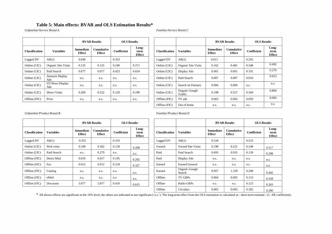
Table 5: Main effects: BVAR and OLS Estimation Results* Unfamiliar/Service Brand A

Familiar/Service Brand C

BVAR Results OLS Results BVAR Results OLS Results

Classification Variables Immediate Effect

Cumulative Effect

Coefficient Long-term Effect


Cumulative Effect


Lagged DV AR(1) 0.646 0.353

Lagged DV AR(1) 0.611 0.292

Online (CIC) Organic Site Visits 0.135 0.135 0.240 0.371 Online (CIC) Organic Site Visits 0.162 0.481 0.348 0.492

Online (CIC) Paid Search 0.077 0.077 0.423 0.654 Online (CIC) Display Ads 0.001 0.001 0.191 0.270

Online (CIC) Amazon Display Ads

n.s. n.s. n.s. n.s. Online (CIC) Paid Search 0.007 0.007 0.016 0.023

Online (CIC) US News Display Ads

n.s. n.s. n.s. n.s. Online (CIC) Search on Partners 0.006 0.006 n.s. n.s.

Online (CIC) Direct Visits 0.200 0.522 0.129 0.199 Online (CIC) Organic Google Traffic

0.198 0.557 0.569 0.804

Offline (FIC) Price n.s. n.s. n.s.. n.s.. Offline (FIC) TV ads 0.003 0.003 0.059 0.083

Offline (FIC) Out of home n.s. n.s. n.s. n.s.

Unfamiliar/Product Brand B

Familiar/Product Brand D



Cumulative Effect Coefficient

Long-term Effect


Cumulative Effect Coefficient

Long-term Effect

Lagged DV AR(1) 0.355 0.333

Lagged DV AR(1) 0.534 0.533

Online (CIC) Web visits 0.190 0.362 0.139 0.208 Owned Owned Site Visits 0.198 0.231 0.148 0.317

Online (CIC) Paid Search n.s. 0.279 n.s. n.s.

Paid Paid Search 0.693 0.935 0.139 0.298

Offline (FIC) Direct Mail 0.010 0.017 0.195 0.292 Paid Display Ads n.s. n.s. n.s. n.s.

Offline (FIC) Fax 0.012 0.012 0.218 0.327

Earned Earned General n.s. n.s. n.s. n.s..

Offline (FIC) Catalog n.s. n.s. n.s.

n.s.

Earned Organic Google Search

0.957 1.339 0.208 0.445

Offline (FIC) eMail n.s. n.s. n.s. n.s. Offline TV GRPs 0.004 0.005 0.153 0.328

Offline (FIC) Discounts 5.877 5.877 0.410 0.615

Offline Radio GRPs n.s. n.s. 0.123 0.263

Offline Circulars 0.003 0.003 0.182 0.390

* All shown effects are significant at the 10% level, the others are indicated as not significant (‘n.s.’). The long-term effect from the OLS estimation is calculated as : short-term estimate / (1- AR coefficient).

37

. Table 6: Full model: BVAR and OLS Estimation Results (with interactions)

Unfamiliar/Service Brand A

Familiar / Service Brand C


Classification Variables Immediate

Effect Cumulative

Effect OLS

Coefficient Long-term

Effect Classification Variables Immediate

Effect Cumulative

Effect OLS


Main Variables Main Variables

Lagged DV AR(1) 0.619 0.430

Lagged DV AR(1) 0.672 0.809

Online (CIC) Organic Site Visits 0.148 0.394 0.185 0.325 Online (CIC) Organic Site Visits 0.557 0.557 0.199 1.042

Online (CIC) Paid Search 0.075 0.096 0.407 0.714 Online (CIC) Display Ads n.s. n.s. 0.117 0.613

Online (CIC) Amazon Display Ads n.s. n.s. n.s.. n.s. Online (CIC) Paid Search 0.009 0.009 0.015 0.079

Online (CIC) US News Display Ads n.s. n.s. n.s. n.s. Online (CIC) Search on Partners 0.008 0.008 0.394 2.063

Online (CIC) Direct Visits 0.167 0.435 0.119 0.209 Online (CIC) Organic Google Traffic 0.898 1.036 0.907 4.749

Offline (FIC) Price n.s. n.s. n.s. n.s. Offline (FIC) TV ads 0.008 0.008 0.165 0.864

All Significant Interactions

Offline (FIC) Out of home n.s. n.s. n.s. n.s.

Offline*Online Price*Organic Site Visits

0.145 0.374 0.094 0.165 All Significant Interactions

Offline*Online Price*Direct Visits 0.168 0.428 n.s. n.s. Online*Offline Display Ads*TV Ads 0.003 0.003 0.103 0.539

Offline*Online Price*Paid Search 0.054 0.069 0.603 1.058 Online*Offline Paid Search*TV Ads 0.003 0.003 0.726 3.801

Online*Online Organic Site Visits*Direct Visits

0.095 0.250 0.079 0.139 Online*Offline Search on Partners*TV Ads

0.003 0.003 0.704 3.686

Online*Online Organic Site Visits*Paid Search

0.055 0.072 0.062 0.109 Online*Offline Org. Google Traffic*TV ads

0.006 0.006 0.203 1.063

Online*Online Direct Visits*Paid Search

0.053 0.070 0.109 0.191 Online*Online Org. Google Traffic*Org. Site Visits

0.451 0.451 n.s. n.s.

Online*Offline TV Ads*Org. Site Visits

0.003 0.003 0.132 0.691

Offline*Offline TV Ads*Out of home 0.001 0.001 n.s. n.s.


Table 6 (cont’d):

Unfamiliar / Product Brand B

Familiar / Product Brand D



Cumulative Effect

OLS Coefficient

Long-term Effect


Cumulative Effect

OLS Coefficient

Long-term Effect

Main Variables Main Variables

Lagged DV AR(1) 0.606 0.289

Lagged DV AR(1) 0.407 0.244

Online (CIC) Web visits 0.225 0.407 0.215 0.302 Online (CIC) Owned Site Visits 0.176 0.102 n.s. n.s.

Online (CIC) Paid Search n.s. 0.199 n.s. n.s. Online (CIC) Paid Search 0.617 0.483 0.284 0.376 Offline (FIC) Direct Mail 0.021 0.036 0.209 0.294 Online (CIC) Display Ads -0.003 -0.002 n.s.

n.s.

Offline (FIC) Fax 0.024 0.024 0.306 0.430 Online (CIC) Earned General n.s. n.s. n.s. n.s.

Offline (FIC) Catalog n.s. n.s. n.s. n.s. Online (CIC) Organic Google Search 0.874 0.766 0.512 0.677 Offline (FIC) eMail 0.008 0.008 n.s. n.s. Offline (FIC) TV GRPs 0.006 0.006 0.297 0.393 Offline (FIC) Discounts 6.601 6.601 0.425 0.598 Offline (FIC) Radio GRPs 0.004 0.004 n.s. n.s.

All Significant Interactions Offline (FIC) Circulars 0.004 0.004 0.174

0.230 Offline*Offline Direct Mail*Fax 0.029 0.029 n.s. n.s. All Significant Interactions

Offline*Offline Direct Mail *Discounts

0.028 0.049 0.777 1.093 Offline*Offline TV*Radio 0.006 0.006 n.s.

n.s.

Offline*Offline Direct Mail*Email 0.011 0.019 0.001 0.001 Offline*Offline TV*Circulars 0.005 0.005 n.s. n.s.

Offline*Online Direct Mail*Web Visits

0.011 0.020 0.171 0.241 Offline*Online TV*Paid Search 0.003 0.003 0.025 0.033

Offline*Online Direct Mail*Paid Search

0.069 0.069 n.s. n.s. Offline*Online Radio*Org. Google Search 0.004 0.004 0.405 0.536

Offline*Offline Fax*Discounts 0.035 0.035 0.094 0.132 Offline*Online Circulars*Owned Site Vis. 0.002 0.002 n.s. n.s.

Offline*Offline Fax*eMail 0.036 0.036 0.004 0.006 Offline*Online Circulars*Paid Search 0.002 0.002 n.s. n.s.

Offline*Online Fax*Web Visits 0.012 0.012 n.s. n.s. Offline*Online Circulars*Org. Google Search 0.003 0.003 1.125 1.488 Offline*Online Discounts*Web Visits 0.461 0.554 n.s. n.s. Online*Online Owned Site Vis.*Paid Search 0.218 0.177 0.089 0.118

Online*Online Paid Search*Web Visits

0.004 0.004 n.s. n.s.s. Online*Online Owned Site Vis.*Org. Google Search

0.286 0.213 n.s.

n.s.

Online*Online

Paid Search*Org. Google Search

0.419 0.336 0.420 0.556


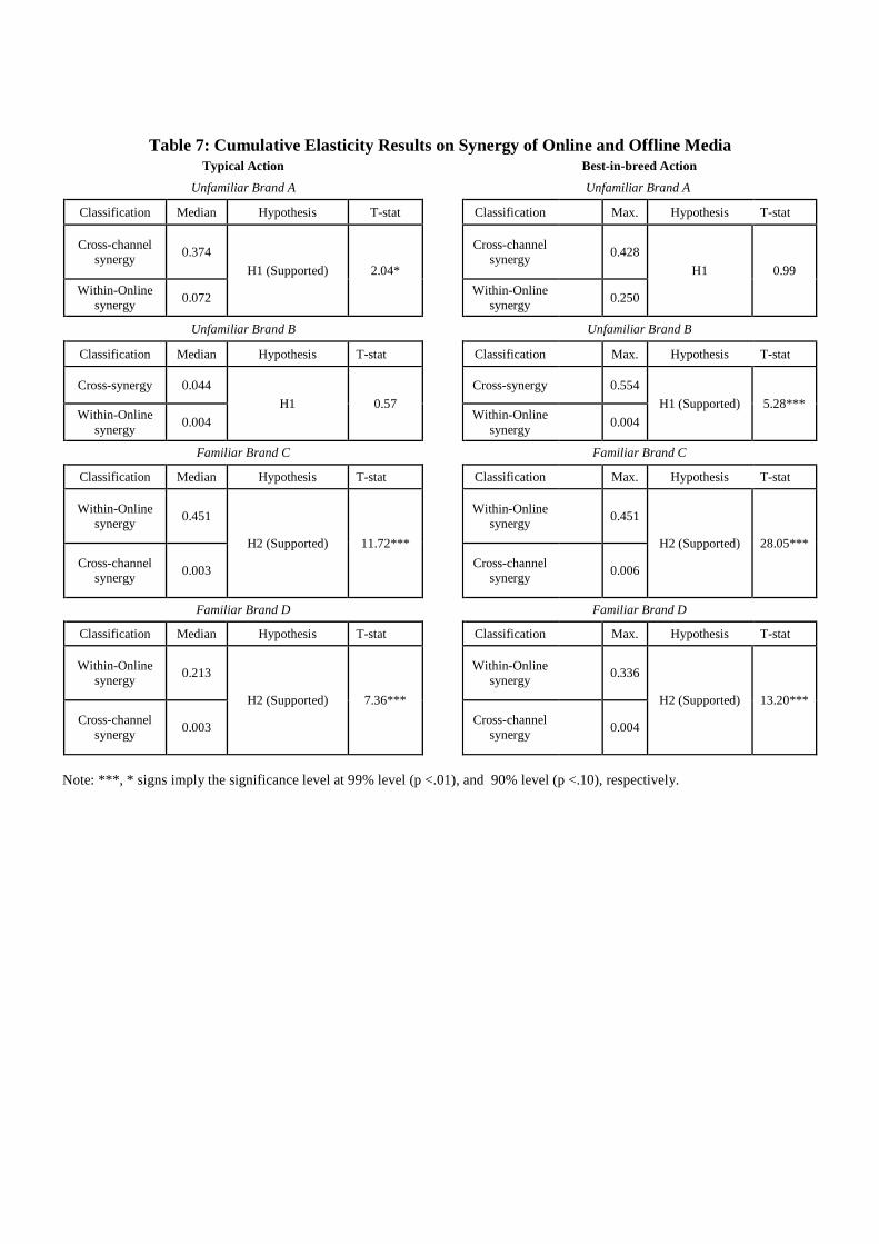
Table 7: Cumulative Elasticity Results on Synergy of Online and Offline Media Typical Action

Best-in-breed Action

Unfamiliar Brand A

Unfamiliar Brand A

Classification Median Hypothesis T-stat Classification Max. Hypothesis T-stat

Cross-channel synergy

0.374

H1 (Supported) 2.04*


0.428

H1 0.99

Within-Online synergy

0.072 Within-Online

synergy 0.250

Unfamiliar Brand B Unfamiliar Brand B

Classification Median Hypothesis T-stat Classification

Max. Hypothesis T-stat

Cross-synergy 0.044

H1 0.57

Cross-synergy 0.554

H1 (Supported) 5.28*** Within-Online

synergy 0.004


0.004

Familiar Brand C

Familiar Brand C

Classification Median Hypothesis T-stat

Classification Max. Hypothesis T-stat


0.451

H2 (Supported) 11.72***


0.451



0.003


0.006

Familiar Brand D

Familiar Brand D

Classification Median Hypothesis T-stat

Classification Max. Hypothesis T-stat


0.213



0.336



0.003


0.004

Note: ***, * signs imply the significance level at 99% level (p <.01), and 90% level (p <.10), respectively.

40

Table 8: Marketing Budget Allocation options for brand B

Media type

Current Allocation

Main Effects Allocation

Allocation Range

Synergies Allocation

Allocation Range

Paid Search 18.30% 90.56%

[68.93% ; 90.89%] 44.52%

[41.66% ; 45.70%]

Direct Mail 66.12% 5.68%

[19.52% ; 4.27%] 36.88%

[39.57% ; 31.31%]

Fax 3.80% 3.76%

[11.55% ; 2.97%] 18.60%

[18.77% ; 20.44%]

Catalog 11.79% 0.00%

[0.00% ; 1.88%] 0.00%

[0.00% ; 2.55%]

* Note: Main effects allocation is based on the point estimates while allocation range is calculated based on +/- one standard error bands.

41

Technical Appendix

A1: Bayesian Vector Autoregression (BVAR) Modeling Steps

Our BVAR modeling approach consists of the following 5 steps:

Step 1: In the first step, we simply consider the unrestricted VAR (k) model and do not

impose restrictions on the coefficients of the VAR model. The optimal lag length is chosen based on

the Schwarz Information Criterion (SIC) which is commonly used in the marketing literature (e.g.

Pauwels et al. 2004). We opt for taking natural logarithm (adding 0.0001 to avoid the log of 0) to

smooth the variables’ distribution and efficiently model diminishing returns. Unit root testing (e.g.

Pauwels et al. 2002) is not applicable to the Bayesian estimation as unit roots do not affect the

likelihood function (Sims, Stock and Watson 1990).

Step 2: After building the VAR model, the second step is to impose the restrictions on the

coefficients of the VAR model by using the set of Minnesota parameters in Eq. (4). In order to find

the best parameters, we consider three values for the weight parameter, w: 0.25, 0.5 and 0.75. For

the tightness parameter �, we assume four different values: 0.5, 0.3, 0.1 and 0.05. The first number

(0.5) is a relatively loose value while the last number (0.05) is a tight value. We chose the lag decay

parameter � to be 1 as suggested by Doan et al. (1984). As a result, we determine the set of the

hyperparameter values, i.e. w, �, �.

Step 3: With the selected parameters from Step 2, we estimate BVAR(k) model10. As

explained in the methodology section, the estimation method is Theil and Goldberger’s mixed

estimation technique.

10 We do not perform Granger causality tests as they are invalid given the Bayesian prior applied to the model (LeSage 1999, page 128).

42

Step 4: We calculate the Generalized Impulse Response Functions (GIRF) (simultaneous

shocking approach) using the formula by Pesaran and Shin (1998). To find the standard errors of

GIRF coefficients we employ the residual-based bootstrap technique. Specifically, we (a) bootstrap

the residuals of the BVAR(k) model, (b) obtain bootstrapped data using the estimated parameters

and the bootstrapped residuals and (c) obtain new BVAR coefficient estimates and GIRF coefficient

estimates using the bootstrapped data. We repeat these steps 500 times and then calculate the

standard errors of the GIRF coefficients.

Step 5: After finding the bootstrapped standard errors, we assess whether each impulse-

response value is significantly different from zero as suggested by VAR-related literature in

marketing (e.g. Pauwels, Hanssens and Siddarth 2002). Finally, we compute the immediate and

cumulative effects based on the significant GIRF estimates.

A2: Budget allocation approach in the absence and presence of synergy

We assume companies aim to maximize profits, which leads to the well-established advice (in the

absence of synergy) that the budget allocation across different media spending should follow their ratio

of marginal elasticities (e.g. Dorfman and Steiner 1954, Wright 2009). The presence of synergy

requires us to update this advice, as we illustrate below. Consider the log-log specification for the

following model without interactions:

� = E + F� + F � + � (Eq.A1)

where � is the residual term with i.i.d. normal. For simplicity, we do not include the time index in the

notation. Taking the first derivative of Eq.A1 with respect to � and � respectively, we obtain the

following marginal elasticities:

GHGIJ = F and GHGIK = F .

43

Then, the budget allocation based on these estimated elasticities becomes LJLJMLK for �, and

LKLJMLK for

� . Now, let us add the interaction (synergy) term to equation A1:

� = E + F� + F � + N(� × � ) + � (Eq.A2)

where � is the residual term with i.i.d. normal.

Taking the first derivative of Eq. A2 with respect to �and � respectively, we get

GHGIJ = F + N� and GHGIK = F + N�

Then, the budget allocation becomes

LJMPJIK(LJMPJIK)M(LKMPJIJ) for �, and

LKMPJIJ(LJMPJIK)M(LKMPJIJ) for � .

Note that marginal elasticity of � changes depending on the level of � . Likewise, the marginal

elasticity of � changes depending on the level of �. We assess the elasticity at the mean values of the

variables. In other words, using the above simple example, our allocation is as follows:

LJMPJIQK(LJMPJIQK)M(LKMPJIQJ) for �, and

LKMPJIQJ(LJMPJIQK)M(LKMPJIQJ) for � . where the notation �Q represents the mean value.

Impact of Brand Familiarity on Online and Offline Media ... of... · The Impact of Brand...

Documents

Transcript of Impact of Brand Familiarity on Online and Offline Media ... of... · The Impact of Brand...