IEEE/ASME TRANSACTIONS ON MECHATRONICS,...

IEEE/ASME TRANSACTIONS ON MECHATRONICS, VOL. 18, NO. 4, AUGUST 2013 1357

Speed-Sensorless Vector Control of a BearinglessInduction Motor With Artificial Neural Network

Inverse Speed ObserverXiaodong Sun, Long Chen, Zebin Yang, and Huangqiu Zhu

Abstract—To effectively reject the influence of speed detectionon system stability and precision for a bearingless induction motor,this paper proposes a novel speed observation scheme using artifi-cial neural network (ANN) inverse method. The inherent subsys-tem consisting of speed and torque winding currents is modeled,and then its inversion is implemented by the ANN. The speed issuccessfully observed via cascading the original subsystem withits inversion. The observed speed is fed back in the speed controlloop, and thus, the speed-sensorless vector drive is realized. Theeffectiveness of this proposed strategy has been demonstrated byexperimental results.

Index Terms—Artificial neural network (ANN) inverse, bearing-less induction motor (BIM), speed-sensorless, vector control.

I. INTRODUCTION

IN recent years, there is an increasing interest in bearinglessmotors around the world [1]–[3]. Due to the similarity of

structure between electric motors [4], [5] and magnetic bear-ings [6], a bearingless motor combine the functions of a motorand a magnetic bearing together within the same stator frame.They can simultaneously produce the radial suspension forceand torque on the rotor so that there is no mechanical contactbetween the stator and rotor. On the one hand, the magneticsuspension offers the advantages of no friction, no abrasion, nolubrication, high rotational speed, and high precision, in com-parison to mechanical contact [7], [8]. On the other hand, abearingless motor has incomparable advantages of small size,light weight, low cost as compared to a conventional tandemstructure consisting of magnetic bearings and a motor. There-fore, bearingless motors are becoming more and more suitable

Manuscript received November 17, 2011; revised February 28, 2012;accepted May 19, 2012. Date of publication June 12, 2012; date of currentversion July 8, 2013. Recommended by Technical Editor G. Yang. This workwas supported in part by the National Natural Science Foundation of China un-der Project 61104016, in part by the Natural Science Foundation of the JiangsuHigher Education Institutions of China under Project 11KJB510002, and in partby the Priority Academic Program Development of Jiangsu Higher EducationInstitutions under Project 201106.

X. Sun was with the School of Electrical and Information Engineering,Jiangsu University, Zhenjiang 212013, China. He is now with the AutomotiveEngineering Research Institute, Jiangsu University, Zhenjiang 212013, China(e-mail: [email protected]).

L. Chen is with the Automotive Engineering Research Institute, Jiangsu Uni-versity, Zhenjiang 212013, China (e-mail: [email protected]).

Z. Yang and H. Zhu are with the School of Electrical and Infor-mation Engineering, Jiangsu University, Zhenjiang 212013, China (e-mail:[email protected]; [email protected]).

Digital Object Identifier 10.1109/TMECH.2012.2202123

for widespread applications, such as high-speed turbo machiner-ies, machine tool spindles, vacuum pumps, blood pumps, com-puter disk drives, energy storage flywheels, etc [9]–[11]. Up tonow, various types of bearingless motors have been proposed,such as bearingless reluctance motors, bearingless inductionmotors (BIMs), bearingless switched reluctance motors, bear-ingless permanent magnet synchronous motors, etc [12]–[16].In these types of bearingless motors, the BIM has been paidmuch attention since its advent because its rotor construction isrelatively simple and robust, and the torque ripples and coggingtorque are less [12].

Since the BIM is a multivariable, nonlinear, and coupled sys-tem, the vector control is a reasonable choice to control its speedindependently from the radial suspension forces. However, forall high-performance vector-controlled BIMs, it is necessary togain the accurate rotational speed information. Normally, thisinformation is achieved by using mechanical sensors such asincremental encoders, which are the most common position-ing transducers used today in industrial applications. Nonethe-less, using mechanical sensors will cause several disadvantages,such as increasing size, cost, maintenance, hardware complexity,electrical susceptibility, and reducing reliability and robustnessof the drive system [17]–[20]. Especially, mechanical sensorsare unsuitable for the inherent high-speed performance of BIMsdue to the unavoidable mechanical contact. Therefore, the con-siderable speed-sensorless control strategies are badly neededfor solving the problems, and the investigation of the speed-sensorless operation is essential for the further development ofBIMs.

For the conventional induction motors, various techniqueshave been proposed to estimate speed for sensorless drives,such as the direct computing method [21], Luenberger observersmethod [22], [23], extended Kalman filter (EKF) method [24],[25], and model reference adaptive system (MRAS) method[26], [27]. The direct computing method is a simplest methodbased on the angular velocity of rotor flux vector and slip calcu-lation using the induction motor model, but the estimated speedaccuracy is not very satisfactory due to the great sensitivity toparameters variations and noise in the drive. The Luenbergerobservers method is a deterministic estimator which assumesa linearized time-invariant motor model. The EKF method canmake the online estimation of states while identifying the mo-tor parameters simultaneously in a relatively short time interval.The Luenberger observers and EKF methods are robust to motorparameters variations or identification errors, but they requirea great number of real-time computations and are much more

1083-4435/$31.00 © 2012 IEEE

1358 IEEE/ASME TRANSACTIONS ON MECHATRONICS, VOL. 18, NO. 4, AUGUST 2013

complicated in practical realization. In the MRAS method, anerror vector is made up from the two models’ outputs whichare both dependent on different motor parameters. By adjust-ing the parameter that influences one of the models, the error isdriven to zero. Compared with the Luenberger observers or EKFmethod, the MRAS method has the advantage in the simplicityof used models. But it is unstable in low speed or around zerospeed running because the model-based estimation technique isdependent on rotor-induced voltages which is very small andeven vanish at zero stator frequency.

In this paper, a novel method of speed-sensorless vector con-trol for a BIM based on artificial neural network (ANN) inversemethod is proposed. The basic principle of the method is toobtain the inverse model of the speed subsystem which consistsof a static ANN and some differentiators, and then to establishthe speed observer by cascading the original subsystem with theANN inverse model. Based on this speed estimation method,the speed-sensorless vector control system of the BIM is set up.Finally, the proposed control strategy is confirmed on a dSPACEDS1104 DSP-based data acquisition and control (DAC) system.

This paper is organized as follows. In Section II, we describethe principle of radial suspension force generation in BIMs.Then, we analyze the inherent subsystem, gain its inverse model,and obtain the speed observer using the inverse system methodin Section III. In Section IV, an ANN inverse speed observer isconstructed. In Section V, the speed-sensorless vector controlsystem of the BIM is set up. In Section VI, experiments arecarried out, and the performance of the BIM drive system isanalyzed and discussed. Finally, some conclusions are given inSection VII.

II. PRINCIPLE OF RADIAL SUSPENSION FORCE GENERATION

Suppose the pole-pair number of torque windings is p1 , andthat of suspension force windings is p2 . When the rotating mag-netic field produced by the two sets of windings satisfy thefollowing three conditions: 1) p2 = p1 ±1, 2) the two magneticfields have the same rotation direction, and 3) the currents intwo sets of windings have the same frequency, then the interac-tive magnetic fields will produce radial suspension forces in theconstant direction.

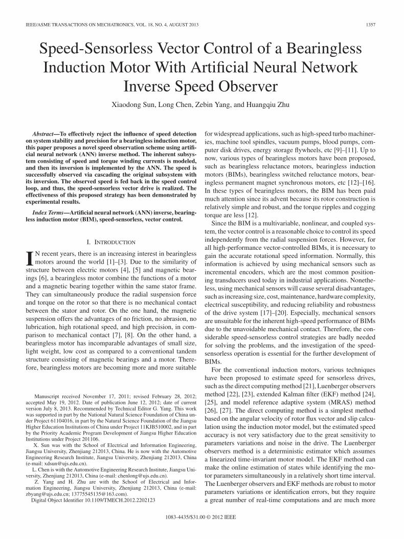
According to the electromagnetic field theory, there are twokinds of magnetic force, namely, Lorentz force and Maxwellforce in the BIM. Besides the electromagnetic torque producedby Lorentz force just as it works in an induction motor, it alsocan generate radial suspension force. Compared with Lorentzforce, Maxwell force, also named magnetic resistance force, isthe main source of the radial suspension force in the BIM. Fig. 1shows the principle of radial suspension force generation. Thefour-pole flux ψ4 and two-pole flux ψ2 are generated by thetorque winding currents i1 and suspension force winding cur-rents i2 in the N4 and N2 turns of stator windings, respectively.Under no-load balanced conditions, if a positive radial suspen-sion force along the x-axis is needed, the torque winding currenti1 and suspension force winding currents i2 are electrified asshown in Fig. 1. The flux density in the airgap 1 is increased,because both fluxes ψ4 and ψ2 are in the same direction. On the

Fig. 1. Principle of radial suspension force generation.

other hand, the flux density in the airgap 2 is decreased becausefluxes ψ4 and ψ2 are in the opposite direction. Therefore, a posi-tive suspension force Fx is produced in the x-axis direction only.If the direction of suspension force winding currents is reversed,the radial suspension force in negative x-axis direction will begenerated. Suspension force Fy in the y-axis direction can beproduced using electrically perpendicular two-pole suspensionforce winding currents distribution. So, the rotor can be sus-pended steadily in the central equilibrium position by adjustingthe magnitude and direction of the suspension force windingcurrents.

III. DESIGN OF THE SPEED OBSERVER

A. Left Inverse System

From the viewpoint of functional analysis, the dynamic modelof a general system can be described as an operator mappingthe inputs into the outputs. We consider a continuous system

∑

(linear or nonlinear) with a p-dimensional input vector u(t) =[u1 , u2 , . . ., up ], a q-dimensional output vector y(t) = [y1 , y2 ,. . ., yq ], and an initial state vector x(t0) = x0 . Let θ : u → y bethe operator describing the aforementioned mapping relation,i.e., [28]

y(•) = θ[x0 ,u(•)] or y = θu. (1)

A system which can realize an inverse mapping from theoutput y to the input u can be defined as an inverse system or aninversion equivalently. In general, according to the difference ofthe function or purpose, the inverse systems can be divided intotwo classes, e.g., right inverse systems and left inverse systems.A right inverse system often serves as an output controller tomake the output y of the original system to follow a givenoutput, while the left inverse system serves as an input observer.Since what we are considered in this paper is studying effectiveobserver approaches, all inverse systems refer to the left inversesystems hereafter if no special statement is given.

Definition 1: Consider a system∑

expressed by (1). AssumeΠ to be another system with y(t) as input and u(t) as output, andit can be described by an operator θ : y → u. If the operator θsatisfies

θθu = θy = u (2)

the system Π is called the inverse system or inversion of theoriginal system

∑, and the original system

∑is invertible [29].

SUN et al.: SPEED-SENSORLESS VECTOR CONTROL OF A BEARINGLESS INDUCTION MOTOR 1359

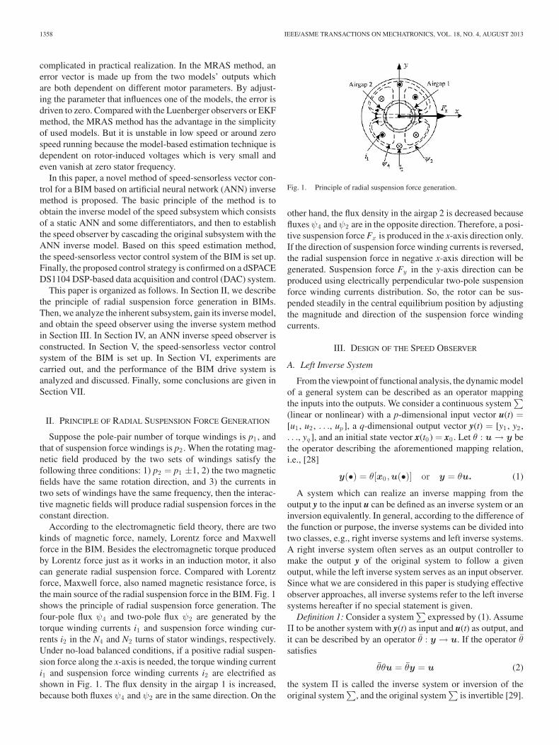
Fig. 2. Compounded identity system.

As shown in Fig. 2, by cascading the original system withsuch an inverse system, the compounded system would becomean identity one, which means that the input of the original systemcan be gained from the output signal of such an inverse system.Since the inversion can completely reproduce the inputs of theoriginal system, it can be treated as a soft sensor (or observer)to estimate some immeasurable variables.

B. Speed Observer Using Inverse System Method

The BIM is essentially an induction motor. For the motor sys-tem controlled inverter, under the assumptions of ignoring thenonlinear and time delay of the inverter, and magnetic circuitsaturation and iron loss of the motor, a three-phase inductionmotor model according to the usual d-axis and q-axis compo-nents in a synchronous rotating frame with rotor flux orientationcan be expressed by [30]

⎧⎪⎪⎪⎪⎪⎪⎪⎪⎪⎪⎪⎪⎪⎪⎪⎪⎪⎪⎪⎨

⎪⎪⎪⎪⎪⎪⎪⎪⎪⎪⎪⎪⎪⎪⎪⎪⎪⎪⎪⎩

is1d =Lm1

σLs1Lr1Trψr1d − (Rs1L

2r1 + Rr1L

2m1)

σLs1L2r1

is1d

+ω1is1q +us1d

σLs1

is1q = − Lm1

σLs1Lr1ωrψr1d − (Rs1L

2r1 + Rr1L

2m1)

σLs1L2r1

is1q

−ω1is1d +us1q

σLs1

ψr1d = − 1Tr

ψr1d +Lm

Tris1d

ωr =p2

1Lm1

JLr1ψr1dis1q −

p1

JTL

(3)where ψr 1d , ψr 1q , is1d , is1q , us1d , us1q are, respectively, thedq-axis components of the rotor flux linkage, stator current,and stator voltage of torque windings, ω1 and ωr are the syn-chronous and rotor electrical angular speed, respectively, Ls1 ,Lr 1 , and Lm 1 are the stator, rotor, and mutual inductances oftorque windings, respectively, Rs1 and Rr 1 are the stator androtor resistances of torque windings, respectively, p1 is the num-ber of pole pairs of torque windings, J is the moment of inertia,Tr = Lr1/Rr1 , and σ = 1 − L2

m1/(Ls1Lr1).

State variables are chosen as

x = [x1 , x2 , x3 , x4 ]T = [is1d , is1q ,ψr1d , ωr ]T . (4)

Input variables are chosen as

u = [u1 , u2 ]T = [us1d , us1q ]T . (5)

Output variables are chosen as

y = [y1 , y2 ]T = [x3 , x4 ]T = [ψr1d , ωr ]T (6)

where the state variables x1 and x2 can be measured directly, andx4 is the to-be-observed variable. In order to observe the rotor

Fig. 3. Speed observation principle based on inverse system method.

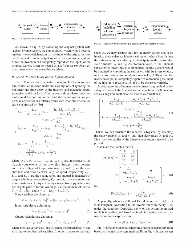
speed x4 , we may assume that, for the motor system (3), in itsinterior, there exists an inherent subsystem whose input is justthe to-be-observed variable x4 , while outputs are the measurablestate variables x1 and x2 . As aforementioned, if the inherentsubsystem is invertible, a compounded identity system wouldbe obtained by cascading the subsystem with its inversion (i.e.,inherent subsystem inversion), as shown in Fig. 3. Therefore, theinversion output is completely capable of reproducing the inputof the inherent subsystem, i.e., the to-be-observed variable.

According to the aforementioned constructing method of thesubsystem model, the first and second equations of (3) are cho-sen as subsystem mathematical model, as rewritten as

⎧⎪⎪⎪⎪⎪⎪⎪⎪⎪⎪⎨

⎪⎪⎪⎪⎪⎪⎪⎪⎪⎪⎩

x1 =Lm1

σLs1Lr1Trx3 −

(Rs1L2r1 + Rr1L

2m1)

σLs1L2r1

x1

+ω1x2 +u1

σLs1

x2 = − Lm1

σLs1Lr1x3x4 −

(Rs1L2r1 + Rr1L

2m1)

σLs1L2r1

x2

−ω1x1 +u2

σLs1.

(7)

That is, we can structure the inherent subsystem by selectingthe state variables x1 and x2 and their derivatives x1 and x2 .Thus, the reversibility of the inherent subsystem is needed to beproved.

Calculate the Jacobin matrix

A (x,u) =

⎡

⎢⎢⎣

∂x1

∂x3

∂x1

∂x4

∂x2

∂x3

∂x2

∂x4

⎤

⎥⎥⎦

=

⎡

⎢⎢⎣

Lm1

σLs1Lr1Tr0

− Lm1x4

σLs1Lr1Tr− Lm1x3

σLs1Lr1Tr

⎤

⎥⎥⎦ . (8)

So,

Det(A(x,u)) = − L2m1

σ2L2s1L

2r1Tr

x3 . (9)

Apparently, when x3 �= 0, and Det(A(x,u)) �= 0, A(x,u)is nonsingular. According to the inverse function theory [31],under the condition Det(A(x,u)) �= 0, the system expressedin (7) is invertible, and based on implicit function theorem, itsinversion can be expressed as

x4 = ϕ(x1 , x2 , x1 , x2 , ω1 ,u). (10)

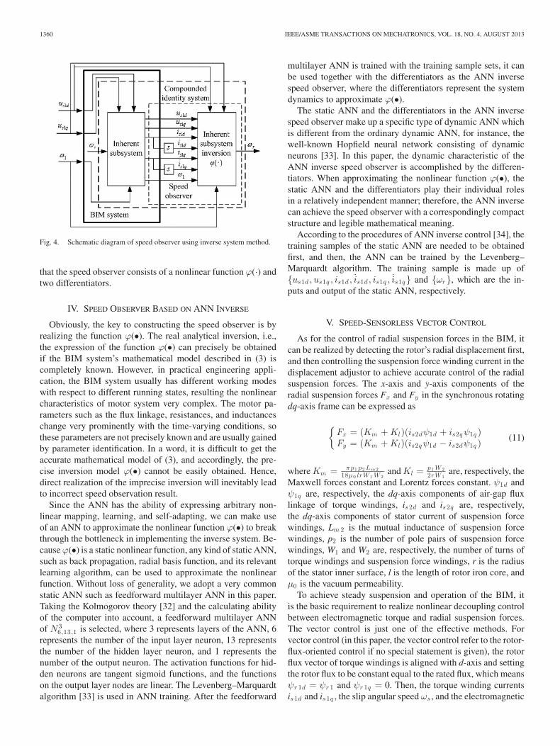
Fig. 4 shows the schematic diagram of rotor speed observationbased on the inverse system method. From Fig. 4, it can be seen


Fig. 4. Schematic diagram of speed observer using inverse system method.

that the speed observer consists of a nonlinear function ϕ(·) andtwo differentiators.

IV. SPEED OBSERVER BASED ON ANN INVERSE

Obviously, the key to constructing the speed observer is byrealizing the function ϕ(•). The real analytical inversion, i.e.,the expression of the function ϕ(•) can precisely be obtainedif the BIM system’s mathematical model described in (3) iscompletely known. However, in practical engineering appli-cation, the BIM system usually has different working modeswith respect to different running states, resulting the nonlinearcharacteristics of motor system very complex. The motor pa-rameters such as the flux linkage, resistances, and inductanceschange very prominently with the time-varying conditions, sothese parameters are not precisely known and are usually gainedby parameter identification. In a word, it is difficult to get theaccurate mathematical model of (3), and accordingly, the pre-cise inversion model ϕ(•) cannot be easily obtained. Hence,direct realization of the imprecise inversion will inevitably leadto incorrect speed observation result.

Since the ANN has the ability of expressing arbitrary non-linear mapping, learning, and self-adapting, we can make useof an ANN to approximate the nonlinear function ϕ(•) to breakthrough the bottleneck in implementing the inverse system. Be-cause ϕ(•) is a static nonlinear function, any kind of static ANN,such as back propagation, radial basis function, and its relevantlearning algorithm, can be used to approximate the nonlinearfunction. Without loss of generality, we adopt a very commonstatic ANN such as feedforward multilayer ANN in this paper.Taking the Kolmogorov theory [32] and the calculating abilityof the computer into account, a feedforward multilayer ANNof N 3

6,13,1 is selected, where 3 represents layers of the ANN, 6represents the number of the input layer neuron, 13 representsthe number of the hidden layer neuron, and 1 represents thenumber of the output neuron. The activation functions for hid-den neurons are tangent sigmoid functions, and the functionson the output layer nodes are linear. The Levenberg–Marquardtalgorithm [33] is used in ANN training. After the feedforward

multilayer ANN is trained with the training sample sets, it canbe used together with the differentiators as the ANN inversespeed observer, where the differentiators represent the systemdynamics to approximate ϕ(•).

The static ANN and the differentiators in the ANN inversespeed observer make up a specific type of dynamic ANN whichis different from the ordinary dynamic ANN, for instance, thewell-known Hopfield neural network consisting of dynamicneurons [33]. In this paper, the dynamic characteristic of theANN inverse speed observer is accomplished by the differen-tiators. When approximating the nonlinear function ϕ(•), thestatic ANN and the differentiators play their individual rolesin a relatively independent manner; therefore, the ANN inversecan achieve the speed observer with a correspondingly compactstructure and legible mathematical meaning.

According to the procedures of ANN inverse control [34], thetraining samples of the static ANN are needed to be obtainedfirst, and then, the ANN can be trained by the Levenberg–Marquardt algorithm. The training sample is made up of{us1d , us1q , is1d , is1d , is1q , is1q} and {ωr}, which are the in-puts and output of the static ANN, respectively.

V. SPEED-SENSORLESS VECTOR CONTROL

As for the control of radial suspension forces in the BIM, itcan be realized by detecting the rotor’s radial displacement first,and then controlling the suspension force winding current in thedisplacement adjustor to achieve accurate control of the radialsuspension forces. The x-axis and y-axis components of theradial suspension forces Fx and Fy in the synchronous rotatingdq-axis frame can be expressed as

{Fx = (Km + Kl)(is2dψ1d + is2qψ1q )Fy = (Km + Kl)(is2qψ1d − is2dψ1q )

(11)

where Km = πp1 p2 Lm 218μ0 lrW 1 W 2

and Kl = p1 W 22rW 1

are, respectively, theMaxwell forces constant and Lorentz forces constant. ψ1d andψ1q are, respectively, the dq-axis components of air-gap fluxlinkage of torque windings, is2d and is2q are, respectively,the dq-axis components of stator current of suspension forcewindings, Lm 2 is the mutual inductance of suspension forcewindings, p2 is the number of pole pairs of suspension forcewindings, W1 and W2 are, respectively, the number of turns oftorque windings and suspension force windings, r is the radiusof the stator inner surface, l is the length of rotor iron core, andμ0 is the vacuum permeability.

To achieve steady suspension and operation of the BIM, itis the basic requirement to realize nonlinear decoupling controlbetween electromagnetic torque and radial suspension forces.The vector control is just one of the effective methods. Forvector control (in this paper, the vector control refer to the rotor-flux-oriented control if no special statement is given), the rotorflux vector of torque windings is aligned with d-axis and settingthe rotor flux to be constant equal to the rated flux, which meansψr 1d = ψr 1 and ψr 1q = 0. Then, the torque winding currentsis1d and is1q , the slip angular speed ωs , and the electromagnetic


torque can be expressed as⎧⎪⎪⎪⎨

⎪⎪⎪⎩

is1d = (Trp1 + 1)ψr1/Lm1

is1q = TeLr1/(p1Lm1ψr1)ωs = ω1 − ωr = Lm1is1q /(Tr1ψr1)Te = p1Lm1is1qψr1/Lr1 .

(12)

From (11), it can be seen that the radial suspension forces arerelated to the air-gap flux of the torque windings; therefore, it canbe used to calculate the radial suspension forces only after theair-gap flux is obtained. According to the relationship betweenair-gap flux and rotor flux, the rotor flux and stator currents oftorque windings are utilized to identify the air-gap flux, and thecalculating formula can be expressed as follows:

{ψ1d = Lm1(ψr1d + Lr1l is1d)/Lr1

ψ1q = Lm1Lr1l is1q /Lr1(13)

where Lr 1l is the rotor leakage inductance of the torque wind-ings. After the airgap is obtained, the suspension force windingcurrents can be determined in accordance with (11). By solving(11), we obtain

[is2d

is2q

]

=1M

[cos ρ − sin ρsin ρ cos ρ

] [Fx

Fy

]

(14)

where M = (Km + Kl)√

ψ21d + ψ2

1q and ρ = arctan (ψ1q /

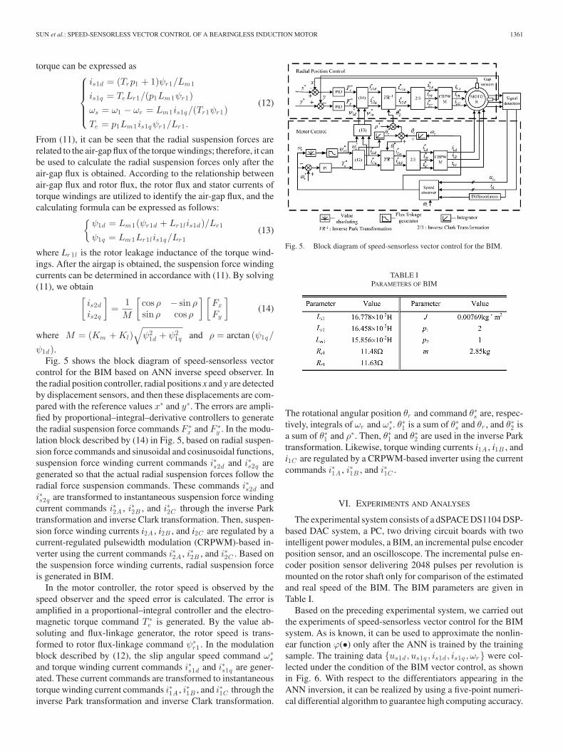
ψ1d).Fig. 5 shows the block diagram of speed-sensorless vector

control for the BIM based on ANN inverse speed observer. Inthe radial position controller, radial positions x and y are detectedby displacement sensors, and then these displacements are com-pared with the reference values x∗ and y∗. The errors are ampli-fied by proportional–integral–derivative controllers to generatethe radial suspension force commands F ∗

x and F ∗y . In the modu-

lation block described by (14) in Fig. 5, based on radial suspen-sion force commands and sinusoidal and cosinusoidal functions,suspension force winding current commands i∗s2d and i∗s2q aregenerated so that the actual radial suspension forces follow theradial force suspension commands. These commands i∗s2d andi∗s2q are transformed to instantaneous suspension force windingcurrent commands i∗2A , i∗2B , and i∗2C through the inverse Parktransformation and inverse Clark transformation. Then, suspen-sion force winding currents i2A , i2B , and i2C are regulated by acurrent-regulated pulsewidth modulation (CRPWM)-based in-verter using the current commands i∗2A , i∗2B , and i∗2C . Based onthe suspension force winding currents, radial suspension forceis generated in BIM.

In the motor controller, the rotor speed is observed by thespeed observer and the speed error is calculated. The error isamplified in a proportional–integral controller and the electro-magnetic torque command T ∗

e is generated. By the value ab-soluting and flux-linkage generator, the rotor speed is trans-formed to rotor flux-linkage command ψ∗

r1 . In the modulationblock described by (12), the slip angular speed command ω∗

s

and torque winding current commands i∗s1d and i∗s1q are gener-ated. These current commands are transformed to instantaneoustorque winding current commands i∗1A , i∗1B , and i∗1C through theinverse Park transformation and inverse Clark transformation.

Fig. 5. Block diagram of speed-sensorless vector control for the BIM.

TABLE IPARAMETERS OF BIM

The rotational angular position θr and command θ∗s are, respec-tively, integrals of ωr and ω∗

s . θ∗1 is a sum of θ∗s and θr , and θ∗2 isa sum of θ∗1 and ρ∗. Then, θ∗1 and θ∗2 are used in the inverse Parktransformation. Likewise, torque winding currents i1A , i1B , andi1C are regulated by a CRPWM-based inverter using the currentcommands i∗1A , i∗1B , and i∗1C .

VI. EXPERIMENTS AND ANALYSES

The experimental system consists of a dSPACE DS1104 DSP-based DAC system, a PC, two driving circuit boards with twointelligent power modules, a BIM, an incremental pulse encoderposition sensor, and an oscilloscope. The incremental pulse en-coder position sensor delivering 2048 pulses per revolution ismounted on the rotor shaft only for comparison of the estimatedand real speed of the BIM. The BIM parameters are given inTable I.

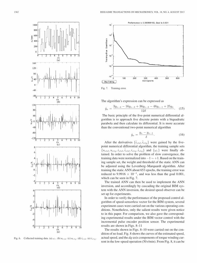
Based on the preceding experimental system, we carried outthe experiments of speed-sensorless vector control for the BIMsystem. As is known, it can be used to approximate the nonlin-ear function ϕ(•) only after the ANN is trained by the trainingsample. The training data {us1d , us1q , is1d , is1q , ωr} were col-lected under the condition of the BIM vector control, as shownin Fig. 6. With respect to the differentiators appearing in theANN inversion, it can be realized by using a five-point numeri-cal differential algorithm to guarantee high computing accuracy.


Fig. 6. Collected training data. (a) ωr . (b) us 1d . (c) us 1q . (d) is 1d . (e) is 1q .

Fig. 7. Training error.

The algorithm’s expression can be expressed as

yn =3yn−4 − 16yn−3 + 36yn−2 − 48yn−1 + 25yn

12δ. (15)

The basic principle of the five-point numerical differential al-gorithm is to approach five discrete points with a biquadraticparabola and then calculate its differential. It is more accuratethan the conventional two-point numerical algorithm

yn =yn − yn−1

δ. (16)

After the derivatives {is1d , is1q} were gained by the five-point numerical differential algorithm, the training sample sets{us1d , us1q , is1d , is1d , is1q , is1q} and {ωr} were finally ob-tained. In order to solve the problem of slow convergence, thetraining data were normalized into−1∼+1. Based on the train-ing sample set, the weight and threshold of the static ANN canbe adjusted using the Levenberg–Marquardt algorithm. Aftertraining the static ANN about 653 epochs, the training error wasreduced to 9.9916 × 10−4 , and was less than the goal 0.001,which can be seen in Fig. 7.

The trained ANN can then be used to implement the ANNinversion, and accordingly by cascading the original BIM sys-tem with the ANN inversion, the desired speed observer can beset up for experiments.

In order to verify the performance of the proposed control al-gorithm of speed-sensorless vector for the BIM system, severalexperiment cases were carried out on the various operating con-ditions. Nonetheless, only the salient results were given noticeto in this paper. For comparison, we also gave the correspond-ing experimental results under the BIM vector control with theincremental pulse encoder position sensor. The experimentalresults are shown in Figs. 8–11

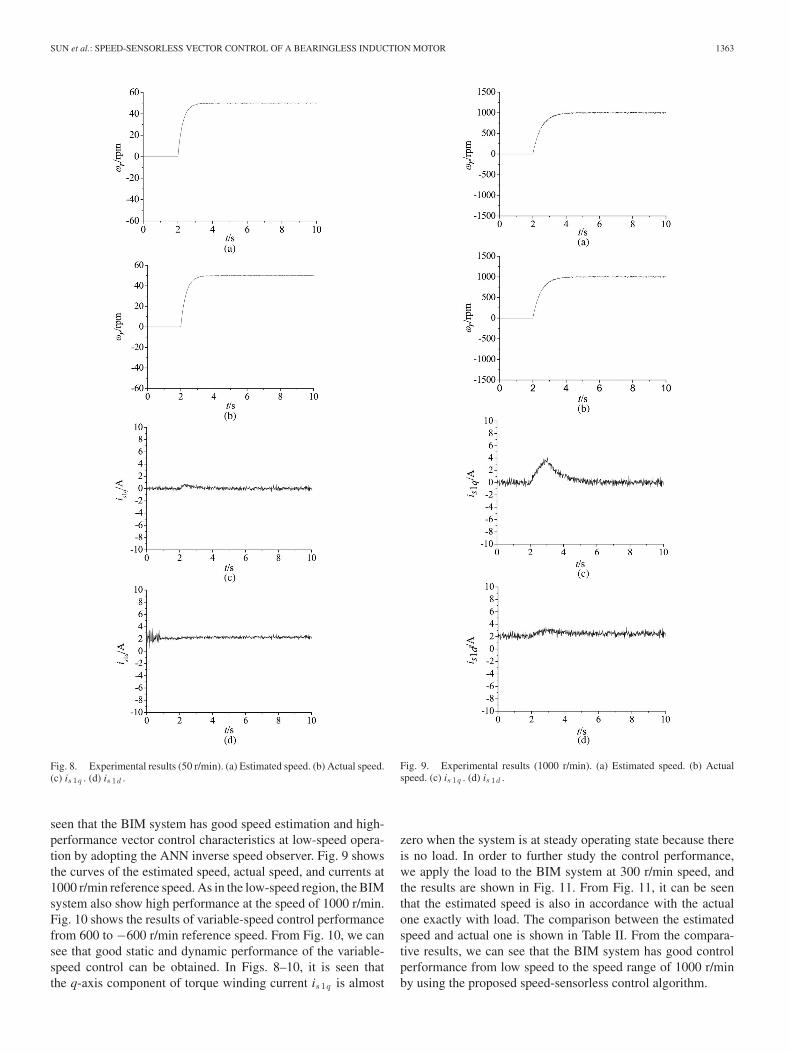
The results shown in Figs. 8–10 were carried out on the con-dition of no load. Fig. 8 shows the curves of the estimated speed,actual speed, and the dq-axis components of torque winding cur-rent in the low-speed operation (50 r/min). From Fig. 8, it can be


Fig. 8. Experimental results (50 r/min). (a) Estimated speed. (b) Actual speed.(c) is 1q . (d) is 1d .

seen that the BIM system has good speed estimation and high-performance vector control characteristics at low-speed opera-tion by adopting the ANN inverse speed observer. Fig. 9 showsthe curves of the estimated speed, actual speed, and currents at1000 r/min reference speed. As in the low-speed region, the BIMsystem also show high performance at the speed of 1000 r/min.Fig. 10 shows the results of variable-speed control performancefrom 600 to −600 r/min reference speed. From Fig. 10, we cansee that good static and dynamic performance of the variable-speed control can be obtained. In Figs. 8–10, it is seen thatthe q-axis component of torque winding current is1q is almost

Fig. 9. Experimental results (1000 r/min). (a) Estimated speed. (b) Actualspeed. (c) is 1q . (d) is 1d .

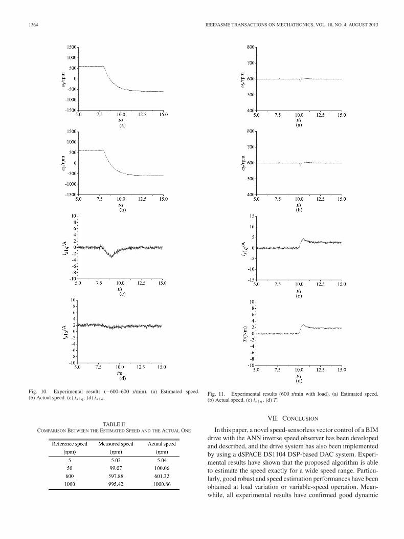
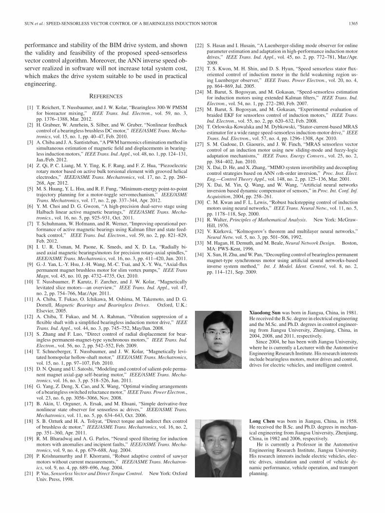
zero when the system is at steady operating state because thereis no load. In order to further study the control performance,we apply the load to the BIM system at 300 r/min speed, andthe results are shown in Fig. 11. From Fig. 11, it can be seenthat the estimated speed is also in accordance with the actualone exactly with load. The comparison between the estimatedspeed and actual one is shown in Table II. From the compara-tive results, we can see that the BIM system has good controlperformance from low speed to the speed range of 1000 r/minby using the proposed speed-sensorless control algorithm.


Fig. 10. Experimental results (−600–600 r/min). (a) Estimated speed.(b) Actual speed. (c) is 1q . (d) is 1d .

TABLE IICOMPARISON BETWEEN THE ESTIMATED SPEED AND THE ACTUAL ONE

Fig. 11. Experimental results (600 r/min with load). (a) Estimated speed.(b) Actual speed. (c) is 1q . (d) T.

VII. CONCLUSION

In this paper, a novel speed-sensorless vector control of a BIMdrive with the ANN inverse speed observer has been developedand described, and the drive system has also been implementedby using a dSPACE DS1104 DSP-based DAC system. Experi-mental results have shown that the proposed algorithm is ableto estimate the speed exactly for a wide speed range. Particu-larly, good robust and speed estimation performances have beenobtained at load variation or variable-speed operation. Mean-while, all experimental results have confirmed good dynamic


performance and stability of the BIM drive system, and shownthe validity and feasibility of the proposed speed-sensorlessvector control algorithm. Moreover, the ANN inverse speed ob-server realized in software will not increase total system cost,which makes the drive system suitable to be used in practicalengineering.

REFERENCES

[1] T. Reichert, T. Nussbaumer, and J. W. Kolar, “Bearingless 300-W PMSMfor bioreactor mixing,” IEEE Trans. Ind. Electron., vol. 59, no. 3,pp. 1376–1388, Mar. 2012.

[2] H. Grabner, W. Amrhein, S. Silber, and W. Gruber, “Nonlinear feedbackcontrol of a bearingless brushless DC motor,” IEEE/ASME Trans. Mecha-tronics, vol. 15, no. 1, pp. 40–47, Feb. 2010.

[3] A. Chiba and J. A. Santisteban, “A PWM harmonics elimination method insimultaneous estimation of magnetic field and displacements in bearing-less induction motors,” IEEE Trans. Ind. Appl., vol. 48, no. 1, pp. 124–131,Jan./Feb. 2012.

[4] Z. Qi, P. C. Liang, M. Y. Ting, K. F. Rang, and F. Z. Hua, “Piezoelectricrotary motor based on active bulk torsional element with grooved helicalelectrodes,” IEEE/ASME Trans. Mechatronics, vol. 17, no. 2, pp. 260–268, Apr. 2012.

[5] M. S. Huang, Y. L. Hsu, and R. F. Fung, “Minimum-energy point-to-pointtrajectory planning for a motor-toggle servomechanism,” IEEE/ASMETrans. Mechatronics, vol. 17, no. 2, pp. 337–344, Apr. 2012.

[6] Y. M. Choi and D. G. Gweon, “A high-precision dual-servo stage usingHalbach linear active magnetic bearings,” IEEE/ASME Trans. Mecha-tronics., vol. 16, no. 5, pp. 925–931, Oct. 2011.

[7] T. Schuhmann, W. Hofmann, and R. Werner, “Improving operational per-formance of active magnetic bearings using Kalman filter and state feed-back control,” IEEE Trans. Ind. Electron., vol. 59, no. 2, pp. 821–829,Feb. 2012.

[8] I. U. R. Usman, M. Paone, K. Smeds, and X. D. Lu, “Radially bi-ased axial magnetic bearings/motors for precision rotary-axial spindles,”IEEE/ASME Trans. Mechatronics, vol. 16, no. 3, pp. 411–420, Jun. 2011.

[9] G.-J. Yan, L.-Y. Hsu, J.-H. Wang, M.-C. Tsai, and X.-Y. Wu, “Axial-fluxpermanent magnet brushless motor for slim vortex pumps,” IEEE TransMagn, vol. 45, no. 10, pp. 4732–4735, Oct. 2010.

[10] T. Nussbaumer, P. Karutz, F. Zurcher, and J. W. Kolar, “Magneticallylevitated slice motors—an overview,” IEEE Trans. Ind. Appl., vol. 47,no. 2, pp. 754–766, Mar./Apr. 2011.

[11] A. Chiba, T. Fukao, O. Ichikawa, M. Oshima, M. Takemoto, and D. G.Dorrell, Magnetic Bearings and Bearingless Drives. Oxford, U.K.:Elsevier, 2005.

[12] A. Chiba, T. Fukao, and M. A. Rahman, “Vibration suppression of aflexible shaft with a simplified bearingless induction motor drive,” IEEETrans. Ind. Appl., vol. 44, no. 3, pp. 745–752, May/Jun. 2008.

[13] S. Zhang and F. Luo, “Direct control of radial displacement for bear-ingless permanent-magnet-type synchronous motors,” IEEE Trans. Ind.Electron., vol. 56, no. 2, pp. 542–552, Feb. 2009.

[14] T. Schneeberger, T. Nussbaumer, and J. W. Kolar, “Magnetically levi-tated homopolar hollow-shaft motor,” IEEE/ASME Trans. Mechatronics,vol. 15, no. 1, pp. 97–107, Feb. 2010.

[15] D. N. Quang and U. Satoshi, “Modeling and control of salient-pole perma-nent magnet axial-gap self-bearing motor,” IEEE/ASME Trans. Mecha-tronics, vol. 16, no. 3, pp. 518–526, Jun. 2011.

[16] G. Yang, Z. Deng, X. Cao, and X. Wang, “Optimal winding arrangementsof a bearingless switched reluctance motor,” IEEE Trans. Power Electron.,vol. 23, no. 6, pp. 3056–3066, Nov. 2008.

[17] B. Akin, U. Orguner, A. Ersak, and M. Ehsani, “Simple derivative-freenonlinear state observer for sensorless ac drives,” IEEE/ASME Trans.Mechatronics, vol. 11, no. 5, pp. 634–643, Oct. 2006.

[18] S. B. Ozturk and H. A. Toliyat, “Direct torque and indirect flux controlof brushless dc motor,” IEEE/ASME Trans. Mechatronics, vol. 16, no. 2,pp. 351–360, Apr. 2011.

[19] R. M. Bharadwaj and A. G. Parlos, “Neural speed filtering for inductionmotors with anomalies and incipient faults,” IEEE/ASME Trans. Mecha-tronics, vol. 9, no. 4, pp. 679–688, Aug. 2004.

[20] P. Krishnamurthy and F. Khorrami, “Robust adaptive control of sawyermotors without current measurements,” IEEE/ASME Trans. Mechatron-ics, vol. 9, no. 4, pp. 689–696, Aug. 2004.

[21] P. Vas, Sensorless Vector and Direct Torque Control. New York: OxfordUniv. Press, 1998.

[22] S. Hasan and I. Husain, “A Luenberger-sliding mode observer for onlineparameter estimation and adaptation in high-performance induction motordrives,” IEEE Trans. Ind. Appl., vol. 45, no. 2, pp. 772–781, Mar./Apr.2009.

[23] T. S. Kwon, M. H. Shin, and D. S. Hyun, “Speed sensorless stator flux-oriented control of induction motor in the field weakening region us-ing Luenberger observer,” IEEE Trans. Power Electron., vol. 20, no. 4,pp. 864–869, Jul. 2005.

[24] M. Barut, S. Bogosyan, and M. Gokasan, “Speed-sensorless estimationfor induction motors using extended Kalman filters,” IEEE Trans. Ind.Electron., vol. 54, no. 1, pp. 272–280, Feb. 2007.

[25] M. Barut, S. Bogosyan, and M. Gokasan, “Experimental evaluation ofbraided EKF for sensorless control of induction motors,” IEEE Trans.Ind. Electron., vol. 55, no. 2, pp. 620–632, Feb. 2008.

[26] T. Orlowska-Kowalska and M. Dybkowski, “Stator-current-based MRASestimator for a wide range speed-sensorless induction-motor drive,” IEEETrans. Ind. Electron., vol. 57, no. 4, pp. 1296–1308, Apr. 2010.

[27] S. M. Gadoue, D. Giaouris, and J. W. Finch, “MRAS sensorless vectorcontrol of an induction motor using new sliding-mode and fuzzy-logicadaptation mechanisms,” IEEE Trans. Energy Convers., vol. 25, no. 2,pp. 384–402, Jun. 2010.

[28] X. Dai, D. He, and X. Zhang, “MIMO system invertibility and decouplingcontrol strategies based on ANN αth-order inversion,” Proc. Inst. Elect.Eng.—Control Theory Appl., vol. 148, no. 2, pp. 125–136, Mar. 2001.

[29] X. Dai, M. Yin, Q. Wang, and W. Wang, “Artificial neural networksinversion based dynamic compensator of sensors,” in Proc. Int. Conf. Inf.Acquisition, 2004, pp. 258–261.

[30] C. M. Kwan and F. L. Lewis, “Robust backstepping control of inductionmotors using neural networks,” IEEE Trans. Neural Netw., vol. 11, no. 5,pp. 1178–118, Sep. 2000.

[31] R. Walter, Principles of Mathematical Analysis. New York: McGraw-Hill, 1976.

[32] V. Kurkova, “Kolmogorov’s theorem and multilayer neural networks,”Neural Netw. vol. 5, no. 3, pp. 501–506, 1992.

[33] M. Hagan, H. Demuth, and M. Beale, Neural Network Design. Boston,MA: PWS-Kent, 1996.

[34] X. Sun, H. Zhu, and W. Pan, “Decoupling control of bearingless permanentmagnet-type synchronous motor using artificial neural networks-basedinverse system method,” Int. J. Model. Ident. Control, vol. 8, no. 2,pp. 114–121, Sep. 2009.

Xiaodong Sun was born in Jiangsu, China, in 1981.He received the B.Sc. degree in electrical engineeringand the M.Sc. and Ph.D. degrees in control engineer-ing from Jiangsu University, Zhenjiang, China, in2004, 2008, and 2011, respectively.

Since 2004, he has been with Jiangsu University,where he is currently a Lecturer with the AutomotiveEngineering Research Institute. His research interestsinclude bearingless motors, motor drives and control,drives for electric vehicles, and intelligent control.

Long Chen was born in Jiangsu, China, in 1958.He received the B.Sc. and Ph.D. degrees in mechan-ical engineering from Jiangsu University, Zhenjiang,China, in 1982 and 2006, respectively.

He is currently a Professor in the AutomotiveEngineering Research Institute, Jiangsu University.His research interests include electric vehicles, elec-tric drives, simulation and control of vehicle dy-namic performance, vehicle operation, and transportplanning.


Zebin Yang was born in Hubei, China, in 1976. Hereceived the B.Sc. and M.Sc. degrees in electrical en-gineering from Jiangsu University, Zhenjiang, China,in 1999 and 2004, respectively, where he is currentlyworking toward the Ph.D. degree.

He is currently an Associate Professor in theSchool of Electrical and Information Engineering,Jiangsu University. His research interests includecontrol engineering and filtering, singular linear sys-tems, and intelligent control of special motors.

Huangqiu Zhu was born in Jiangsu, China, in 1964.He received the Ph.D. degree in mechanical engi-neering from Nanjing University of Aeronautics andAstronautics, Nanjing, China, in 2000.

He is currently a Professor in the School of Elec-trical and Information Engineering, Jiangsu Univer-sity, Zhenjiang, China. His research interests includemagnetic bearings, magnetic suspension (bearing-less) motors, motor’s movement control, etc.

IEEE/ASME TRANSACTIONS ON MECHATRONICS,...

Documents

Transcript of IEEE/ASME TRANSACTIONS ON MECHATRONICS,...