IBM SPSS Statistics 25 Brief Guide - KendallHunt · 2 IBM SPSS Statistics 26 Brief Guide Running an...

IBM SPSS Statistics 26 Brief Guide

IBM

NoteBefore using this information and the product it supports, read the information in “Notices” on page 83.

Product Information

This edition applies to version 26, release 0, modification 0 of IBM SPSS Statistics Base Integrated Student Edition and to all subsequent releases and modifications until otherwise indicated in new editions.

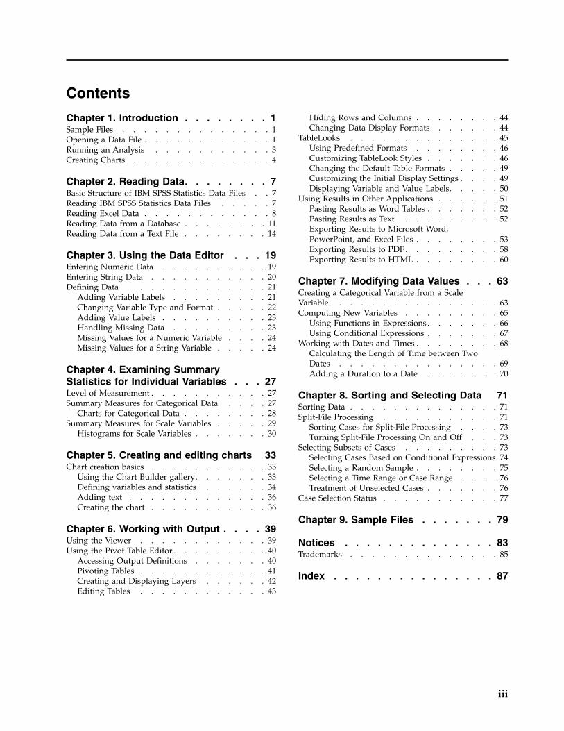
Contents

Chapter 1. Introduction . . . . . . . . 1Sample Files . . . . . . . . . . . . . . 1Opening a Data File . . . . . . . . . . . . 1Running an Analysis . . . . . . . . . . . 3Creating Charts . . . . . . . . . . . . . 4

Chapter 2. Reading Data. . . . . . . . 7Basic Structure of IBM SPSS Statistics Data Files . . 7Reading IBM SPSS Statistics Data Files . . . . . 7Reading Excel Data . . . . . . . . . . . . 8Reading Data from a Database . . . . . . . . 11Reading Data from a Text File . . . . . . . . 14

Chapter 3. Using the Data Editor . . . 19Entering Numeric Data . . . . . . . . . . 19Entering String Data . . . . . . . . . . . 20Defining Data . . . . . . . . . . . . . 21

Adding Variable Labels . . . . . . . . . 21Changing Variable Type and Format . . . . . 22Adding Value Labels . . . . . . . . . . 23Handling Missing Data . . . . . . . . . 23Missing Values for a Numeric Variable . . . . 24Missing Values for a String Variable . . . . . 24

Chapter 4. Examining SummaryStatistics for Individual Variables . . . 27Level of Measurement . . . . . . . . . . . 27Summary Measures for Categorical Data . . . . 27

Charts for Categorical Data . . . . . . . . 28Summary Measures for Scale Variables . . . . . 29

Histograms for Scale Variables . . . . . . . 30

Chapter 5. Creating and editing charts 33Chart creation basics . . . . . . . . . . . 33

Using the Chart Builder gallery. . . . . . . 33Defining variables and statistics . . . . . . 34Adding text . . . . . . . . . . . . . 36Creating the chart . . . . . . . . . . . 36

Chapter 6. Working with Output . . . . 39Using the Viewer . . . . . . . . . . . . 39Using the Pivot Table Editor . . . . . . . . . 40

Accessing Output Definitions . . . . . . . 40Pivoting Tables . . . . . . . . . . . . 41Creating and Displaying Layers . . . . . . 42Editing Tables . . . . . . . . . . . . 43

Hiding Rows and Columns . . . . . . . . 44Changing Data Display Formats . . . . . . 44

TableLooks . . . . . . . . . . . . . . 45Using Predefined Formats . . . . . . . . 46Customizing TableLook Styles . . . . . . . 46Changing the Default Table Formats . . . . . 49Customizing the Initial Display Settings . . . . 49Displaying Variable and Value Labels. . . . . 50

Using Results in Other Applications . . . . . . 51Pasting Results as Word Tables . . . . . . . 52Pasting Results as Text . . . . . . . . . 52Exporting Results to Microsoft Word,PowerPoint, and Excel Files . . . . . . . . 53Exporting Results to PDF . . . . . . . . . 58Exporting Results to HTML . . . . . . . . 60

Chapter 7. Modifying Data Values . . . 63Creating a Categorical Variable from a ScaleVariable . . . . . . . . . . . . . . . 63Computing New Variables . . . . . . . . . 65

Using Functions in Expressions . . . . . . . 66Using Conditional Expressions . . . . . . . 67

Working with Dates and Times . . . . . . . . 68Calculating the Length of Time between TwoDates . . . . . . . . . . . . . . . 69Adding a Duration to a Date . . . . . . . 70

Chapter 8. Sorting and Selecting Data 71Sorting Data . . . . . . . . . . . . . . 71Split-File Processing . . . . . . . . . . . 71

Sorting Cases for Split-File Processing . . . . 73Turning Split-File Processing On and Off . . . 73

Selecting Subsets of Cases . . . . . . . . . 73Selecting Cases Based on Conditional Expressions 74Selecting a Random Sample . . . . . . . . 75Selecting a Time Range or Case Range . . . . 76Treatment of Unselected Cases . . . . . . . 76

Case Selection Status . . . . . . . . . . . 77

Chapter 9. Sample Files . . . . . . . 79

Notices . . . . . . . . . . . . . . 83Trademarks . . . . . . . . . . . . . . 85

Index . . . . . . . . . . . . . . . 87

iii

iv IBM SPSS Statistics 26 Brief Guide

Chapter 1. Introduction

This guide will show you how to use many of the available features. It is designed to provide astep-by-step, hands-on guide. All of the files shown in the examples are installed with the application sothat you can follow along, performing the same analyses and obtaining the same results shown here.

If you want detailed examples of various statistical analysis techniques, try the step-by-step Case Studies,available from the Help menu.

Sample FilesMost of the examples that are presented here use the data file demo.sav. This data file is a fictitious surveyof several thousand people, containing basic demographic and consumer information.

If you are using the Student version, your version of demo.sav is a representative sample of the originaldata file, reduced to meet the 1,500-case limit. Results that you obtain using that data file will differ fromthe results shown here.

The sample files installed with the product can be found in the Samples subdirectory of the installationdirectory. There is a separate folder within the Samples subdirectory for each of the following languages:English, French, German, Italian, Japanese, Korean, Polish, Russian, Simplified Chinese, Spanish, andTraditional Chinese.

Not all sample files are available in all languages. If a sample file is not available in a language, thatlanguage folder contains an English version of the sample file.

Opening a Data FileTo open a data file:1. From the menus choose:

File > Open > Data...

A dialog box for opening files is displayed.By default, IBM® SPSS® Statistics data files (.sav extension) are displayed.This example uses the file demo.sav.

© Copyright IBM Corporation 1989, 2019 1

The data file is displayed in the Data Editor. In Data View, if you put the mouse cursor on a variablename (the column headings), a more descriptive variable label is displayed (if a label has beendefined for that variable).By default, the actual data values are displayed. To display labels:

2. From the menus choose:

View > Value Labels

Alternatively, you can use the Value Labels button on the toolbar.

Descriptive value labels are now displayed to make it easier to interpret the responses.

Figure 1. demo.sav file in Data Editor

Figure 2. Value Labels button

Figure 3. Value labels displayed in the Data Editor

2 IBM SPSS Statistics 26 Brief Guide

Running an AnalysisIf you have any add-on options, the Analyze menu contains a list of reporting and statistical analysiscategories.

We will start by creating a simple frequency table (table of counts). This example requires Statistics BaseEdition.1. From the menus choose:

Analyze > Descriptive Statistics > Frequencies...

The Frequencies dialog box is displayed.

An icon next to each variable provides information about data type and level of measurement.

Numeric String Date Time

Scale (Continuous) n/a

Ordinal

Nominal

If the variable label and/or name appears truncated in the list, the complete label/name is displayedwhen the cursor is positioned over it. The variable name inccat is displayed in square brackets afterthe descriptive variable label. Income category in thousands is the variable label. If there were novariable label, only the variable name would appear in the list box.You can resize dialog boxes just like windows, by clicking and dragging the outside borders orcorners. For example, if you make the dialog box wider, the variable lists will also be wider.In the dialog box, you choose the variables that you want to analyze from the source list on the leftand drag and drop them into the Variable(s) list on the right. The OK button, which runs the analysis,is disabled until at least one variable is placed in the Variable(s) list.

Figure 4. Frequencies dialog box

Chapter 1. Introduction 3

In many dialogs, you can obtain additional information by right-clicking any variable name in the listand selecting Variable Information from the pop-up menu.

2. Click Gender [gender] in the source variable list and drag the variable into the target Variable(s) list.3. Click Income category in thousands [inccat] in the source list and drag it to the target list.

4. Click OK to run the procedure.

Results are displayed in the Viewer window.

Figure 5. Variables selected for analysis

Figure 6. Frequency table of income categories

Creating ChartsAlthough some statistical procedures can create charts, you can also use the Graphs menu to create charts.

For example, you can create a chart that shows the relationship between wireless telephone service and PDA (personal digital assistant) ownership.


1. From the menus choose:Graphs > Chart Builder...

2. Click the Gallery tab (if it is not selected).3. Click Bar (if it is not selected).4. Drag the Clustered Bar icon onto the canvas, which is the large area above the Gallery.5. Scroll down the Variables list, right-click Wireless service [wireless], and then choose Nominal as its

measurement level.6. Drag the Wireless service [wireless] variable to the x axis.7. Right-click Owns PDA [ownpda] and choose Nominal as its measurement level.8. Drag the Owns PDA [ownpda] variable to the cluster drop zone in the upper right corner of the

canvas.9. Click OK to create the chart.

Figure 7. Chart Builder dialog box with completed drop zones

Chapter 1. Introduction 5

The bar chart is displayed in the Viewer. The chart shows that people with wireless phone service are farmore likely to have PDAs than people without wireless service.

You can edit charts and tables by double-clicking them in the contents pane of the Viewer window, andyou can copy and paste your results into other applications. Those topics will be covered later.

Figure 8. Bar chart displayed in Viewer window


Chapter 2. Reading Data

Data can be entered directly, or it can be imported from a number of different sources. The processes forreading data stored in IBM SPSS Statistics data files; spreadsheet applications, such as Microsoft Excel;database applications, such as Microsoft Access; and text files are all discussed in this chapter.

Basic Structure of IBM SPSS Statistics Data Files

IBM SPSS Statistics data files are organized by cases (rows) and variables (columns). In this data file,cases represent individual respondents to a survey. Variables represent responses to each question askedin the survey.

Reading IBM SPSS Statistics Data FilesIBM SPSS Statistics data files, which have a .sav file extension, contain your saved data.1. From the menus choose:

File > Open > Data...

2. Browse to and open demo.sav. See the topic Chapter 9, “Sample Files,” on page 79 for moreinformation.

The data are now displayed in the Data Editor.

Figure 9. Data Editor


Reading Excel DataRather than typing all of your data directly into the Data Editor, you can read data from applicationssuch as Microsoft Excel. You can also read column headings as variable names.1. From the menus choose:

File > Import Data > Excel

2. Go to the Samples\English folder and select demo.xlsx.The Read Excel File dialog displays a preview of the data file. The contents of the first sheet in the fileare displayed. If the file has multiple sheets, you can select the sheet from the list.You can see that some of the string values for Gender have leading spaces. Some of the values forMaritalStatus are displayed as periods (.).

Figure 10. Opened data file


3. Make sure Read variable names from the first row of data is selected. If the column headings do notconform to variable name rules, they are converted to valid variable names. The original columnheadings are saved as variable labels.

4. Select Remove leading spaces from string values.5. Deselect Percentage of values that determine data type.

Figure 11. Read Excel File dialog

Chapter 2. Reading Data 9

The string value "no answer" is now displayed in the cells that were system-missing. If there is nopercentage of values parameter and the column contains a mix of data type, the variable is read as astring data type. All values are preserved, but numeric values are treated as string values.

6. Select (check) Percentage of values that determine data type to treat MaritalStatus as a numericvariable.

7. Click OK to read the Excel file.

The data now appear in the Data Editor, with the column headings used as variable names. Sincevariable names can't contain spaces, the spaces from the original column headings are removed. Forexample, the column heading"Marital Status" is converted to the variable MaritalStatus. The originalcolumn heading is retained as a variable label.


Related information:Chapter 9, “Sample Files,” on page 79

Reading Data from a DatabaseData from database sources are easily imported using the Database Wizard. Any database that usesODBC (Open Database Connectivity) drivers can be read directly after the drivers are installed. ODBCdrivers for many database formats are supplied on the installation CD. Additional drivers can beobtained from third-party vendors. One of the most common database applications, Microsoft Access, isdiscussed in this example.

Note: This example is specific to Microsoft Windows and requires an ODBC driver for Access. TheMicrosoft Access ODBC driver only works with the 32-bit version of IBM SPSS Statistics. The steps aresimilar on other platforms but may require a third-party ODBC driver for Access.1. From the menus choose:

File > Import Data > Database > New Query...

Figure 12. Imported Excel data


2. Select MS Access Database from the list of data sources and click Next.3. Click Browse to navigate to the Access database file that you want to open.4. Open demo.mdb. See the topic Chapter 9, “Sample Files,” on page 79 for more information.5. Click OK in the login dialog box.

In the next step, you can specify the tables and variables that you want to import.

Figure 13. Database Wizard Welcome dialog box


6. Drag the entire demo table to the Retrieve Fields In This Order list.7. Click Next.

In the next step, you can select which records (cases) to import.If you do not want to import all cases, you can import a subset of cases (for example, males olderthan 30), or you can import a random sample of cases from the data source. For large data sources,you may want to limit the number of cases to a small, representative sample to reduce theprocessing time.

8. Click Next to continue.Field names are used to create variable names. If necessary, the names are converted to validvariable names. The original field names are preserved as variable labels. You can also change thevariable names before importing the database.

Figure 14. Select Data step


9. Click the Recode to Numeric cell in the Gender field. This option converts string variables to integervariables and retains the original value as the value label for the new variable.

10. Click Next to continue.The SQL statement created from your selections in the Database Wizard appears in the Results step.This statement can be executed now or saved to a file for later use.

11. Click Finish to import the data.

All of the data in the Access database that you selected to import are now available in the Data Editor.

Reading Data from a Text FileText files represent another common source of data. Many spreadsheet programs and databases can savetheir contents in one of many text file formats. Comma- or tab-delimited files refer to rows of data thatuse commas or tabs to indicate each variable. In this example, the data is tab-delimited.1. From the menus choose:

File > Import Data > Text Data

2. Go to the Samples\English folder and select demo.txt.

Figure 15. Define Variables step


The Text Import Wizard guides you through the process of defining how the specified text file isinterpreted.

3. In Step 1, you can choose a predefined format or create a new format in the wizard. Select No.4. Click Next to continue.

As stated earlier, this file uses tab-delimited formatting. Also, the variable names are defined on thetop line of this file.

5. In step 2 of the wizard, select Delimited to indicate that the file has a delimited formatting structure.6. Select Yes to indicate that the file includes variable names at the top of the file.7. Click Next to continue.8. In step 3, enter 2 for the line number where the first case of data begins (because variable names are

on the first line).9. Keep the default values for the remainder of this step, and click Next to continue.

The Data preview in Step 4 provides you with a quick way to ensure that the file is read correctly10. Select Tab and deselect the other options for delimiters. Space is selected by default because the file

contains spaces. For this file, spaces are part of the data values, not delimiters. You need to deselectSpace to read the file correctly.

11. Select Remove leading spaces for string values. Spaces at the start of string values affect how stringvalues are evaluated in expressions. In this file, some values for Gender have leading spaces that arenot part of the value. If you do not remove those spaces, a value of " f" is treated as a different valuethan "f".

Figure 16. Text Import Wizard: Step 1 of 6


12. Click Next to continue.Because the variable names are modified to conform to naming rules, step 5 gives you theopportunity to edit any undesirable names.Data types can be defined here as well. For example, you can change Income to dollar currencyformat.To change a data type:

13. In the Data preview, select Income.14. Select Dollar from the Data format drop-down list.

Figure 17. Text Import Wizard: Step 4 of 6


The variable MaritalStatus contains both string and numeric values. Less than five percent of thevalues are strings. With the default setting of 95% for Percentage of values that determine theAutomatic data format, the variable is treated as numeric and the string values are set tosystem-missing. If no data format meets the percentage value, the variable is treated as a stringvariable. If you change the setting to 100, all values are preserved, but all numeric values are treatedas strings.

15. Click Next to continue.16. Leave the default selections in the last step, and click Finish to import the data.

Figure 18. Change the data type


Chapter 3. Using the Data Editor

The Data Editor displays the contents of the active data file. The information in the Data Editor consistsof variables and cases.v In Data View, columns represent variables, and rows represent cases (observations).v In Variable View, each row is a variable, and each column is an attribute that is associated with that

variable.

Variables are used to represent the different types of data that you have compiled. A common analogy isthat of a survey. The response to each question on a survey is equivalent to a variable. Variables come inmany different types, including numbers, strings, currency, and dates.

Entering Numeric DataData can be entered into the Data Editor, which may be useful for small data files or for making minoredits to larger data files.1. Click the Variable View tab at the bottom of the Data Editor window.

You need to define the variables that will be used. In this case, only three variables are needed: age,marital status, and income.

2. In the first row of the first column, type age.3. In the second row, type marital.4. In the third row, type income.

New variables are automatically given a Numeric data type.If you don't enter variable names, unique names are automatically created. However, these namesare not descriptive and are not recommended for large data files.

5. Click the Data View tab to continue entering the data.

Figure 19. Variable names in Variable View

19

The names that you entered in Variable View are now the headings for the first three columns inData View.Begin entering data in the first row, starting at the first column.

6. In the age column, type 55.7. In the marital column, type 1.8. In the income column, type 72000.9. Move the cursor to the second row of the first column to add the next subject's data.

10. In the age column, type 53.11. In the marital column, type 0.12. In the income column, type 153000.

Currently, the age and marital columns display decimal points, even though their values are intendedto be integers. To hide the decimal points in these variables:

13. Click the Variable View tab at the bottom of the Data Editor window.14. In the Decimals column of the age row, type 0 to hide the decimal.15. In the Decimals column of the marital row, type 0 to hide the decimal.

Entering String DataNon-numeric data, such as strings of text, can also be entered into the Data Editor.1. Click the Variable View tab at the bottom of the Data Editor window.2. In the first cell of the first empty row, type sex for the variable name.3. Click the Type cell next to your entry.4. Click the button on the right side of the Type cell to open the Variable Type dialog box.5. Select String to specify the variable type.6. Click OK to save your selection and return to the Data Editor.

Figure 20. Values entered in Data View


Defining DataIn addition to defining data types, you can also define descriptive variable labels and value labels forvariable names and data values. These descriptive labels are used in statistical reports and charts.

Adding Variable LabelsLabels are meant to provide descriptions of variables. These descriptions are often longer versions ofvariable names. Labels can be up to 255 bytes. These labels are used in your output to identify thedifferent variables.1. Click the Variable View tab at the bottom of the Data Editor window.2. In the Label column of the age row, type Respondent's Age.3. In the Label column of the marital row, type Marital Status.4. In the Label column of the income row, type Household Income.5. In the Label column of the sex row, type Gender.

Figure 21. Variable Type dialog box

Chapter 3. Using the Data Editor 21

Changing Variable Type and FormatThe Type column displays the current data type for each variable. The most common data types arenumeric and string, but many other formats are supported. In the current data file, the income variable isdefined as a numeric type.1. Click the Type cell for the income row, and then click the button on the right side of the cell to open

the Variable Type dialog box.2. Select Dollar.

The formatting options for the currently selected data type are displayed.3. For the format of the currency in this example, select $###,###,###.4. Click OK to save your changes.

Figure 22. Variable labels entered in Variable View

Figure 23. Variable Type dialog box


Adding Value LabelsValue labels provide a method for mapping your variable values to a string label. In this example, thereare two acceptable values for the marital variable. A value of 0 means that the subject is single, and avalue of 1 means that he or she is married.1. Click the Values cell for the marital row, and then click the button on the right side of the cell to open

the Value Labels dialog box.The value is the actual numeric value.The value label is the string label that is applied to the specified numeric value.

2. Type 0 in the Value field.3. Type Single in the Label field.4. Click Add to add this label to the list.

5. Type 1 in the Value field, and type Married in the Label field.6. Click Add, and then click OK to save your changes and return to the Data Editor.

These labels can also be displayed in Data View, which can make your data more readable.7. Click the Data View tab at the bottom of the Data Editor window.8. From the menus choose:

View > Value Labels

The labels are now displayed in a list when you enter values in the Data Editor. This setup has thebenefit of suggesting a valid response and providing a more descriptive answer.

If the Value Labels menu item is already active (with a check mark next to it), choosing Value Labelsagain will turn off the display of value labels.

Handling Missing DataMissing or invalid data are generally too common to ignore. Survey respondents may refuse to answercertain questions, may not know the answer, or may answer in an unexpected format. If you don't filteror identify these data, your analysis may not provide accurate results.

For numeric data, empty data fields or fields containing invalid entries are converted to system-missing,which is identifiable by a single period.

Figure 24. Value Labels dialog box


The reason a value is missing may be important to your analysis. For example, you may find it useful todistinguish between those respondents who refused to answer a question and those respondents whodidn't answer a question because it was not applicable.

Missing Values for a Numeric Variable1. Click the Variable View tab at the bottom of the Data Editor window.2. Click the Missing cell in the age row, and then click the button on the right side of the cell to open

the Missing Values dialog box.In this dialog box, you can specify up to three distinct missing values, or you can specify a range ofvalues plus one additional discrete value.

3. Select Discrete missing values.4. Type 999 in the first text box and leave the other two text boxes empty.5. Click OK to save your changes and return to the Data Editor.

Now that the missing data value has been added, a label can be applied to that value.6. Click the Values cell in the age row, and then click the button on the right side of the cell to open the

Value Labels dialog box.7. Type 999 in the Value field.8. Type No Response in the Label field.9. Click Add to add this label to your data file.

10. Click OK to save your changes and return to the Data Editor.

Missing Values for a String VariableMissing values for string variables are handled similarly to the missing values for numeric variables.However, unlike numeric variables, empty fields in string variables are not designated as system-missing.Rather, they are interpreted as an empty string.1. Click the Variable View tab at the bottom of the Data Editor window.2. Click the Missing cell in the sex row, and then click the button on the right side of the cell to open

the Missing Values dialog box.3. Select Discrete missing values.4. Type NR in the first text box.

Missing values for string variables are case sensitive. So, a value of nr is not treated as a missingvalue.

5. Click OK to save your changes and return to the Data Editor.Now you can add a label for the missing value.

6. Click the Values cell in the sex row, and then click the button on the right side of the cell to open theValue Labels dialog box.

Figure 25. Missing Values dialog box


7. Type NR in the Value field.8. Type No Response in the Label field.9. Click Add to add this label to your project.

10. Click OK to save your changes and return to the Data Editor.


Chapter 4. Examining Summary Statistics for IndividualVariables

This section discusses simple summary measures and how the level of measurement of a variableinfluences the types of statistics that should be used. We will use the data file demo.sav. See the topicChapter 9, “Sample Files,” on page 79 for more information.

Level of MeasurementDifferent summary measures are appropriate for different types of data, depending on the level ofmeasurement:

Categorical. Data with a limited number of distinct values or categories (for example, gender or maritalstatus). Also referred to as qualitative data. Categorical variables can be string (alphanumeric) data ornumeric variables that use numeric codes to represent categories (for example, 0 = Unmarried and 1 =Married). There are two basic types of categorical data:v Nominal. Categorical data where there is no inherent order to the categories. For example, a job

category of sales is not higher or lower than a job category of marketing or research.v Ordinal. Categorical data where there is a meaningful order of categories, but there is not a

measurable distance between categories. For example, there is an order to the values high, medium, andlow, but the "distance" between the values cannot be calculated.

Scale. Data measured on an interval or ratio scale, where the data values indicate both the order ofvalues and the distance between values. For example, a salary of $72,195 is higher than a salary of$52,398, and the distance between the two values is $19,797. Also referred to as quantitative orcontinuous data.

Summary Measures for Categorical DataFor categorical data, the most typical summary measure is the number or percentage of cases in eachcategory. The mode is the category with the greatest number of cases. For ordinal data, the median (thevalue at which half of the cases fall above and below) may also be a useful summary measure if there isa large number of categories.

The Frequencies procedure produces frequency tables that display both the number and percentage ofcases for each observed value of a variable.1. From the menus choose:

Analyze > Descriptive Statistics > Frequencies...

Note: This feature requires Statistics Base Edition.2. Select Owns PDA [ownpda] and Owns TV [owntv] and move them into the Variable(s) list.

27


The frequency tables are displayed in the Viewer window. The frequency tables reveal that only 20.4% ofthe people own PDAs, but almost everybody owns a TV (99.0%). These might not be interestingrevelations, although it might be interesting to find out more about the small group of people who do notown televisions.

Charts for Categorical DataYou can graphically display the information in a frequency table with a bar chart or pie chart.1. Open the Frequencies dialog box again. (The two variables should still be selected.)

You can use the Dialog Recall button on the toolbar to quickly return to recently used procedures.

Figure 26. Categorical variables selected for analysis

Figure 27. Frequency tables


2. Click Charts.3. Select Bar charts and then click Continue.4. Click OK in the main dialog box to run the procedure.

In addition to the frequency tables, the same information is now displayed in the form of bar charts,making it easy to see that most people do not own PDAs but almost everyone owns a TV.

Summary Measures for Scale VariablesThere are many summary measures available for scale variables, including:v Measures of central tendency. The most common measures of central tendency are the mean

(arithmetic average) and median (value at which half the cases fall above and below).v Measures of dispersion. Statistics that measure the amount of variation or spread in the data include

the standard deviation, minimum, and maximum.1. Open the Frequencies dialog box again.2. Click Reset to clear any previous settings.3. Select Household income in thousands [income] and move it into the Variable(s) list.4. Click Statistics.5. Select Mean, Median, Std. deviation, Minimum, and Maximum.6. Click Continue.7. Deselect Display frequency tables in the main dialog box. (Frequency tables are usually not useful

for scale variables since there may be almost as many distinct values as there are cases in the datafile.)

Figure 28. Dialog Recall button

Figure 29. Bar chart

Chapter 4. Examining Summary Statistics for Individual Variables 29


The Frequencies Statistics table is displayed in the Viewer window.

In this example, there is a large difference between the mean and the median. The mean is almost 25,000greater than the median, indicating that the values are not normally distributed. You can visually checkthe distribution with a histogram.

Histograms for Scale Variables1. Open the Frequencies dialog box again.2. Click Charts.3. Select Histograms and With normal curve.4. Click Continue, and then click OK in the main dialog box to run the procedure.

Figure 30. Frequencies Statistics table


The majority of cases are clustered at the lower end of the scale, with most falling below 100,000. Thereare, however, a few cases in the 500,000 range and beyond (too few to even be visible without modifyingthe histogram). These high values for only a few cases have a significant effect on the mean but little orno effect on the median, making the median a better indicator of central tendency in this example.

Figure 31. Histogram

Chapter 4. Examining Summary Statistics for Individual Variables 31

Chapter 5. Creating and editing charts

You can create and edit a wide variety of chart types. In this chapter, we will create and edit bar charts.You can apply the principles to any chart type.

Chart creation basicsTo demonstrate the basics of chart creation, we will create a bar chart of mean income for different levelsof job satisfaction. This example uses the data file demo.sav. See the topic Chapter 9, “Sample Files,” onpage 79 for more information.1. From the menus choose:

Graphs > Chart Builder...

The Chart Builder dialog box is an interactive window that allows you to preview how a chart will lookwhile you build it.

Figure 32. Chart Builder dialog box

Using the Chart Builder gallery1. Click the Gallery tab if it is not selected.


The Gallery includes many different predefined charts, which are organized by chart type. The BasicElements tab also provides basic elements (such as axes and graphic elements) for creating chartsfrom scratch, but it's easier to use the Gallery.

2. Click Bar if it is not selected.Icons representing the available bar charts in the Gallery appear in the dialog box. The picturesshould provide enough information to identify the specific chart type. If you need more information,you can also display a ToolTip description of the chart by pausing your cursor over an icon.

3. Drag the icon for the simple bar chart onto the "canvas," which is the large area above the Gallery.The Chart Builder displays a preview of the chart on the canvas. Note that the data used to draw thechart are not your actual data. They are example data.

Figure 33. Bar chart on Chart Builder canvas

Defining variables and statisticsAlthough there is a chart on the canvas, it is not complete because there are no variables or statistics to control how tall the bars are and to specify which variable category corresponds to each bar. You can't have a chart without variables and statistics. You add variables by dragging them from the Variables list, which is located to the left of the canvas.

A variable's measurement level is important in the Chart Builder. You are going to use the Job satisfaction variable on the x axis. However, the icon (which looks like a ruler) next to the variable indicates that its measurement level is defined as scale. To create the correct chart, you must use a categorical


measurement level. Instead of going back and changing the measurement level in the Variable View, youcan change the measurement level temporarily in the Chart Builder.1. Right-click Job satisfaction in the Variables list and choose Ordinal. Ordinal is an appropriate

measurement level because the categories in Job satisfaction can be ranked by level of satisfaction. Notethat the icon changes after you change the measurement level.

2. Now drag Job satisfaction from the Variables list to the x axis drop zone.The y axis drop zone defaults to the Count statistic. If you want to use another statistic (such aspercentage or mean), you can easily change it. You will not use either of these statistics in thisexample, but we will review the process in case you need to change this statistic at another time.

3. Click the Element Properties tab in the side bar of the Chart Builder. (If the side bar is not displayed,click the button in the upper right corner of the Chart Builder to display the side bar.)

Element Properties allows you to change the properties of the various chart elements. These elementsinclude the graphic elements (such as the bars in the bar chart) and the axes on the chart. Select oneof the elements in the Edit Properties of list to change the properties associated with that element.Also note the red X located to the right of the list. This button deletes a graphic element from thecanvas. Because Bar1 is selected, the properties shown apply to graphic elements, specifically the bargraphic element.The Statistic drop-down list shows the specific statistics that are available. The same statistics areusually available for every chart type. Be aware that some statistics require that the y axis drop zonecontains a variable.

4. Drag Household income in thousands from the Variables list to the y axis drop zone. Because the variableon the y axis is scalar and the x axis variable is categorical (ordinal is a type of categoricalmeasurement level), the y axis drop zone defaults to the Mean statistic. These are the variables andstatistics you want, so there is no need to change the element properties.

Figure 34. Element Properties

Chapter 5. Creating and editing charts 35

Adding textYou can also add titles and footnotes to the chart.1. Click the Titles/Footnotes tab.2. Select Title 1.

The title appears on the canvas with the label T1.3. In the Element Properties tab, select Title 1 in the Edit Properties of list.4. In the Content text box, type Income by Job Satisfaction. This is the text that the title will display.

Creating the chart1. Click OK to create the bar chart.

Figure 35. Title 1 displayed on canvas


The bar chart reveals that respondents who are more satisfied with their jobs tend to have higherhousehold incomes.

Figure 36. Bar chart

Chapter 5. Creating and editing charts 37

Chapter 6. Working with Output

The results from running a statistical procedure are displayed in the Viewer. The output produced can bestatistical tables, charts, graphs, or text, depending on the choices you make when you run the procedure.This section uses the files viewertut.spv and demo.sav. See the topic Chapter 9, “Sample Files,” on page 79for more information.

Using the Viewer

The Viewer window is divided into two panes. The outline pane contains an outline of all of theinformation stored in the Viewer. The contents pane contains statistical tables, charts, and text output.

Use the scroll bars to navigate through the window's contents, both vertically and horizontally. For easiernavigation, click an item in the outline pane to display it in the contents pane.1. Click and drag the right border of the outline pane to change its width.

An open book icon in the outline pane indicates that it is currently visible in the Viewer, although itmay not currently be in the visible portion of the contents pane.

2. To hide a table or chart, double-click its book icon in the outline pane.The open book icon changes to a closed book icon, signifying that the information associated with it isnow hidden.

3. To redisplay the hidden output, double-click the closed book icon.You can also hide all of the output from a particular statistical procedure or all of the output in theViewer.

4. Click the box with the minus sign (−) to the left of the procedure whose results you want to hide, orclick the box next to the topmost item in the outline pane to hide all of the output.The outline collapses, visually indicating that these results are hidden.You can also change the order in which the output is displayed.

5. In the outline pane, click the items that you want to move.

Figure 37. Viewer


6. Drag the selected items to a new location in the outline.

You can also move output items by clicking and dragging them in the contents pane.

Using the Pivot Table EditorThe results from most statistical procedures are displayed in pivot tables.

Accessing Output DefinitionsMany statistical terms are displayed in the output. Definitions of these terms can be accessed directly inthe Viewer.1. Double-click the Owns PDA * Gender * Internet Crosstabulation table.2. Right-click Expected Count and choose What's This? from the pop-up menu.

The definition is displayed in a pop-up window.

Figure 38. Reordered output in the Viewer


Pivoting TablesThe default tables produced may not display information as neatly or as clearly as you would like. Withpivot tables, you can transpose rows and columns ("flip" the table), adjust the order of data in a table,and modify the table in many other ways. For example, you can change a short, wide table into a long,thin one by transposing rows and columns. Changing the layout of the table does not affect the results.Instead, it's a way to display your information in a different or more desirable manner.1. If it's not already activated, double-click the Owns PDA * Gender * Internet Crosstabulation table to

activate it.2. If the Pivoting Trays window is not visible, from the menus choose:

Pivot > Pivoting Trays

Pivoting trays provide a way to move data between columns, rows, and layers.

Figure 39. Pop-up definition

Chapter 6. Working with Output 41

3. Drag the Statistics element from the Row dimension to the Column dimension, below Gender. Thetable is immediately reconfigured to reflect your changes.The order of the elements in the pivoting tray reflects the order of the elements in the table.

4. Drag and drop the Owns PDA element before the Internet element in the row dimension to reverse theorder of these two rows.

Figure 40. Pivoting trays

Figure 41. Swap rows

Creating and Displaying LayersLayers can be useful for large tables with nested categories of information. By creating layers, you simplify the look of the table, making it easier to read.1. Drag the Gender element from the Column dimension to the Layer dimension.


To display a different layer, select a category from the drop-down list in the table.

Editing TablesUnless you've taken the time to create a custom TableLook, pivot tables are created with standardformatting. You can change the formatting of any text within a table. Formats that you can changeinclude font name, font size, font style (bold or italic), and color.1. Double-click the Level of education table.2. If the Formatting toolbar is not visible, from the menus choose:

View > Toolbar

3. Click the title text, Level of education.4. From the drop-down list of font sizes on the toolbar, choose 12.5. To change the color of the title text, click the text color tool and choose a new color.

You can also edit the contents of tables and labels. For example, you can change the title of this table.6. Double-click the title.7. Type Education Level for the new label.

Note: If you change the values in a table, totals and other statistics are not recalculated.

Figure 42. Gender pivot icon in the Layer dimension

Figure 43. Reformatted title text in the pivot table


Hiding Rows and ColumnsSome of the data displayed in a table may not be useful or it may unnecessarily complicate the table.Fortunately, you can hide entire rows and columns without losing any data.1. If it's not already activated, double-click the Education Level table to activate it.2. Click Valid Percent column label to select it.3. From the Edit menu or the right-click pop-up menu choose:

Select > Data and Label Cells

4. From the View menu choose Hide or from the right-click pop-up menu choose Hide Category.The column is now hidden but not deleted.

To redisplay the column:5. From the menus choose:

View > Show All

Rows can be hidden and displayed in the same way as columns.

Changing Data Display FormatsYou can easily change the display format of data in pivot tables.1. If it's not already activated, double-click the Education Level table to activate it.2. Click the Percent column label to select it.3. From the Edit menu or the right-click pop-up menu choose:

Select > Data Cells

4. From the Format menu or the right-click pop-up menu choose Cell Properties.5. Click the Format Value tab.6. Type 0 in the Decimals field to hide all decimal points in this column.

Figure 44. Valid Percent column hidden in table


You can also change the data type and format in this dialog box.7. Select the type that you want from the Category list, and then select the format for that type in the

Format list.8. Click OK or Apply to apply your changes.

The decimals are now hidden in the Percent column.

TableLooksThe format of your tables is a critical part of providing clear, concise, and meaningful results. If yourtable is difficult to read, the information contained within that table may not be easily understood.

Figure 45. Cell Properties, Format Value tab

Figure 46. Decimals hidden in Percent column


Using Predefined Formats1. Double-click the Marital status table.2. From the menus choose:

Format > TableLooks...

The TableLooks dialog box lists a variety of predefined styles. Select a style from the list to preview itin the Sample window on the right.

You can use a style as is, or you can edit an existing style to better suit your needs.3. To use an existing style, select one and click OK.

Customizing TableLook StylesYou can customize a format to fit your specific needs. Almost all aspects of a table can be customized,from the background color to the border styles.1. Double-click the Marital status table.2. From the menus choose:

Format > TableLooks...

3. Select the style that is closest to the format you want and click Edit Look.4. Click the Cell Formats tab to view the formatting options.

Figure 47. TableLooks dialog box


The formatting options include font name, font size, style, and color. Additional options includealignment, text and background colors, and margin sizes.The Sample window on the right provides a preview of how the formatting changes affect yourtable. Each area of the table can have different formatting styles. For example, you probablywouldn't want the title to have the same style as the data. To select a table area to edit, you caneither choose the area by name in the Area drop-down list, or you can click the area that you wantto change in the Sample window.

5. Select Data from the Area drop-down list.6. Select a new color from the Background drop-down palette.7. Then select a new text color.

The Sample window shows the new style.

Figure 48. Table Properties dialog box


8. Click OK to return to the TableLooks dialog box.You can save your new style, which allows you to apply it to future tables easily.

9. Click Save As.10. Navigate to the target directory and enter a name for your new style in the File Name text box.11. Click Save.12. Click OK to apply your changes and return to the Viewer.

The table now contains the custom formatting that you specified.

Figure 49. Changing table cell formats

Figure 50. Custom TableLook


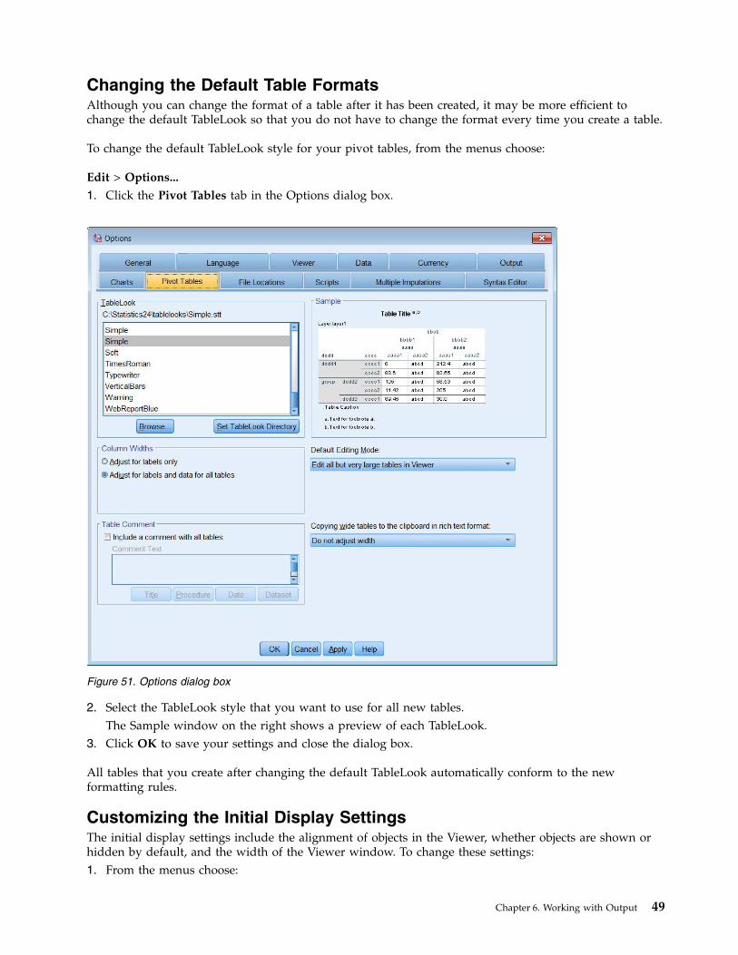
Changing the Default Table FormatsAlthough you can change the format of a table after it has been created, it may be more efficient tochange the default TableLook so that you do not have to change the format every time you create a table.

To change the default TableLook style for your pivot tables, from the menus choose:

Edit > Options...

1. Click the Pivot Tables tab in the Options dialog box.

2. Select the TableLook style that you want to use for all new tables.The Sample window on the right shows a preview of each TableLook.

3. Click OK to save your settings and close the dialog box.

All tables that you create after changing the default TableLook automatically conform to the newformatting rules.

Customizing the Initial Display SettingsThe initial display settings include the alignment of objects in the Viewer, whether objects are shown orhidden by default, and the width of the Viewer window. To change these settings:1. From the menus choose:

Figure 51. Options dialog box


Edit > Options...

2. Click the Viewer tab.

The settings are applied on an object-by-object basis. For example, you can customize the way chartsare displayed without making any changes to the way tables are displayed. Simply select the objectthat you want to customize, and make the changes.

3. Click the Title icon to display its settings.4. Click Center to display all titles in the (horizontal) center of the Viewer.

You can also hide elements, such as the log and warning messages, that tend to clutter your output.Double-clicking on an icon automatically changes that object's display property.

5. Double-click the Warnings icon to hide warning messages in the output.6. Click OK to save your changes and close the dialog box.

Displaying Variable and Value LabelsIn most cases, displaying the labels for variables and values is more effective than displaying the variablename or the actual data value. There may be cases, however, when you want to display both the namesand the labels.1. From the menus choose:

Edit > Options...

Figure 52. Viewer options


2. Click the Output Labels tab.

You can specify different settings for the outline and contents panes. For example, to show labels inthe outline and variable names and data values in the contents:

3. In the Pivot Table Labeling group, select Names from the Variables in Labels drop-down list to showvariable names instead of labels.

4. Then, select Values from the Variable Values in Labels drop-down list to show data values instead oflabels.

Subsequent tables produced in the session will reflect these changes.

Using Results in Other ApplicationsYour results can be used in many applications. For example, you may want to include a table or chart ina presentation or report.

Figure 53. Pivot Table Labeling settings

Figure 54. Variable names and values displayed


The following examples are specific to Microsoft Word, but they may work similarly in other wordprocessing applications.

Pasting Results as Word TablesYou can paste pivot tables into Word as native Word tables. All table attributes, such as font sizes andcolors, are retained. Because the table is pasted in the Word table format, you can edit it in Word just likeany other table.1. Click a table in the Viewer to select it.2. From the menus choose:

Edit > Copy

3. Open your word processing application.4. From the word processor's menus choose:

Edit > Paste Special...

5. Select Formatted Text (RTF) in the Paste Special dialog box.6. Click OK to paste your results into the current document.

The table is now displayed in your document. You can apply custom formatting, edit the data, and resizethe table to fit your needs.

Pasting Results as TextPivot tables can be copied to other applications as plain text. Formatting styles are not retained in thismethod, but you can edit the table data after you paste it into the target application.1. Click a table in the Viewer to select it.2. From the menus choose:

Edit > Copy

3. Open your word processing application.4. From the word processor's menus choose:

Edit > Paste Special...

5. Select Unformatted Text in the Paste Special dialog box.6. Click OK to paste your results into the current document.


Each column of the table is separated by tabs. You can change the column widths by adjusting the tabstops in your word processing application.

Exporting Results to Microsoft Word, PowerPoint, and Excel FilesYou can export results to a Microsoft Word , PowerPoint, or Excel file. You can export selected items orall items in the Viewer. This section uses the files msouttut.spv and demo.sav. See the topic Chapter 9,“Sample Files,” on page 79 for more information.

Note: Export to PowerPoint is available only on Windows operating systems and is not available with theStudent Version.

In the Viewer's outline pane, you can select specific items that you want to export or export all items orall visible items.

Figure 55. Pivot table displayed in Word


1. From the Viewer menus choose:File > Export...

Instead of exporting all objects in the Viewer, you can choose to export only visible objects (openbooks in the outline pane) or those that you selected in the outline pane. If you did not select anyitems in the outline pane, you do not have the option to export selected objects.

Figure 56. Viewer


2. In the Objects to Export group, select All.3. From the Type drop-down list select Word/RTF file (*.doc).4. Click OK to generate the Word file.

When you open the resulting file in Word, you can see how the results are exported. Notes, which are notvisible objects, appear in Word because you chose to export all objects.

Pivot tables become Word tables, with all of the formatting of the original pivot table retained, includingfonts, colors, borders, and so on.

Figure 57. Export Output dialog box


Charts are included in the Word document as graphic images.

Text output is displayed in the same font used for the text object in the Viewer. For proper alignment,text output should use a fixed-pitch (monospaced) font.

Figure 58. Pivot tables in Word

Figure 59. Charts in Word


Note: Export to PowerPoint is available only on Windows operating systems and is not available with theStudent Version.

If you export to an Excel file, results are exported differently.

Pivot table rows, columns, and cells become Excel rows, columns, and cells.

Figure 60. Text output in Word

Figure 61. Output.xls in Excel


Each line in the text output is a row in the Excel file, with the entire contents of the line contained in asingle cell.

Exporting Results to PDFYou can export all or selected items in the Viewer to a PDF (portable document format) file.1. From the menus in the Viewer window that contains the result you want to export to PDF choose:

File > Export...

2. In the Export Output dialog box, from the Export Format File Type drop-down list choose PortableDocument Format.

Figure 62. Text output in Excel


v The outline pane of the Viewer document is converted to bookmarks in the PDF file for easynavigation.

v Page size, orientation, margins, content and display of page headers and footers, and printed chartsize in PDF documents are controlled by page setup options (File menu, Page Setup in the Viewerwindow).

v The resolution (DPI) of the PDF document is the current resolution setting for the default or currentlyselected printer (which can be changed using Page Setup). The maximum resolution is 1200 DPI. If theprinter setting is higher, the PDF document resolution will be 1200 DPI. Note: High-resolutiondocuments may yield poor results when printed on lower-resolution printers.

Figure 63. Export Output dialog box


Exporting Results to HTMLYou can also export results to HTML (hypertext markup language). When saving as HTML, allnon-graphic output is exported into a single HTML file.

Figure 64. PDF file with bookmarks

Figure 65. Output.htm in Web browser

When you export to HTML, charts can be exported as well, but not to a single file.


Each chart will be saved as a file in a format that you specify, and references to these graphics files willbe placed in the HTML. There is also an option to export all charts (or selected charts) to separategraphics files.

Figure 66. Chart in HTML


Chapter 7. Modifying Data Values

The data you start with may not always be organized in the most useful manner for your analysis orreporting needs. For example, you may want to:v Create a categorical variable from a scale variable.v Combine several response categories into a single category.v Create a new variable that is the computed difference between two existing variables.v Calculate the length of time between two dates.

This chapter uses the data file demo.sav. See the topic Chapter 9, “Sample Files,” on page 79 for moreinformation.

Creating a Categorical Variable from a Scale VariableSeveral categorical variables in the data file demo.sav are, in fact, derived from scale variables in that datafile. For example, the variable inccat is simply income grouped into four categories. This categoricalvariable uses the integer values 1–4 to represent the following income categories (in thousands): less than$25, $25–$49, $50–$74, and $75 or higher.

To create the categorical variable inccat:1. From the menus in the Data Editor window choose:

Transform > Visual Binning...

In the initial Visual Binning dialog box, you select the scale and/or ordinal variables for which youwant to create new, binned variables. Binning means taking two or more contiguous values andgrouping them into the same category.Since Visual Binning relies on actual values in the data file to help you make good binning choices,it needs to read the data file first. Since this can take some time if your data file contains a largenumber of cases, this initial dialog box also allows you to limit the number of cases to read ("scan").This is not necessary for our sample data file. Even though it contains more than 6,000 cases, it doesnot take long to scan that number of cases.

2. Drag and drop Household income in thousands [income] from the Variables list into the Variables to Binlist, and then click Continue.


3. In the main Visual Binning dialog box, select Household income in thousands [income] in the ScannedVariable List.A histogram displays the distribution of the selected variable (which in this case is highly skewed).

4. Enter inccat2 for the new binned variable name and Income category [in thousands] for thevariable label.

5. Click Make Cutpoints.6. Select Equal Width Intervals.

7. Enter 25 for the first cutpoint location, 3 for the number of cutpoints, and 25 for the width.The number of binned categories is one greater than the number of cutpoints. So in this example, thenew binned variable will have four categories, with the first three categories each containing rangesof 25 (thousand) and the last one containing all values above the highest cutpoint value of 75(thousand).

8. Click Apply.The values now displayed in the grid represent the defined cutpoints, which are the upper endpointsof each category. Vertical lines in the histogram also indicate the locations of the cutpoints.By default, these cutpoint values are included in the corresponding categories. For example, the firstvalue of 25 would include all values less than or equal to 25. But in this example, we wantcategories that correspond to less than 25, 25–49, 50–74, and 75 or higher.

9. In the Upper Endpoints group, select Excluded (<).

10. Then click Make Labels.

Figure 67. Main Visual Binning dialog box


This automatically generates descriptive value labels for each category. Since the actual valuesassigned to the new binned variable are simply sequential integers starting with 1, the value labelscan be very useful.You can also manually enter or change cutpoints and labels in the grid, change cutpoint locations bydragging and dropping the cutpoint lines in the histogram, and delete cutpoints by draggingcutpoint lines off of the histogram.

11. Click OK to create the new, binned variable.

The new variable is displayed in the Data Editor. Since the variable is added to the end of the file, it isdisplayed in the far right column in Data View and in the last row in Variable View.

Computing New VariablesUsing a wide variety of mathematical functions, you can compute new variables based on highlycomplex equations. In this example, however, we will simply compute a new variable that is thedifference between the values of two existing variables.

The data file demo.sav contains a variable for the respondent's current age and a variable for the numberof years at current job. It does not, however, contain a variable for the respondent's age at the time he orshe started that job. We can create a new variable that is the computed difference between current ageand number of years at current job, which should be the approximate age at which the respondentstarted that job.1. From the menus in the Data Editor window choose:

Transform > Compute Variable...

2. For Target Variable, enter jobstart.3. Select Age in years [age] in the source variable list and click the arrow button to copy it to the Numeric

Expression text box.

Figure 68. Automatically generated value labels

Chapter 7. Modifying Data Values 65

4. Click the minus (–) button on the calculator pad in the dialog box (or press the minus key on thekeyboard).

5. Select Years with current employer [employ] and click the arrow button to copy it to the expression.

Note: Be careful to select the correct employment variable. There is also a recoded categorical versionof the variable, which is not what you want. The numeric expression should be age–employ, notage–empcat.

Figure 69. Compute Variable dialog box

6. Click OK to compute the new variable.

The new variable is displayed in the Data Editor. Since the variable is added to the end of the file, it is displayed in the far right column in Data View and in the last row in Variable View.

Using Functions in ExpressionsYou can also use predefined functions in expressions. More than 70 built-in functions are available, including:v Arithmetic functionsv Statistical functionsv Distribution functionsv Logical functionsv Date and time aggregation and extraction functionsv Missing-value functionsv Cross-case functionsv String functions


Functions are organized into logically distinct groups, such as a group for arithmetic operations andanother for computing statistical metrics. For convenience, a number of commonly used system variables,such as $TIME (current date and time), are also included in appropriate function groups.

Pasting a Function into an Expression

To paste a function into an expression:1. Position the cursor in the expression at the point where you want the function to appear.2. Select the appropriate group from the Function group list. The group labeled All provides a listing of

all available functions and system variables.3. Double-click the function in the Functions and Special Variables list (or select the function and click

the arrow adjacent to the Function group list).

The function is inserted into the expression. If you highlight part of the expression and then insert thefunction, the highlighted portion of the expression is used as the first argument in the function.

Editing a Function in an Expression

The function is not complete until you enter the arguments, represented by question marks in the pastedfunction. The number of question marks indicates the minimum number of arguments required tocomplete the function.1. Highlight the question mark(s) in the pasted function.2. Enter the arguments. If the arguments are variable names, you can paste them from the variable list.

Using Conditional ExpressionsYou can use conditional expressions (also called logical expressions) to apply transformations to selectedsubsets of cases. A conditional expression returns a value of true, false, or missing for each case. If theresult of a conditional expression is true, the transformation is applied to that case. If the result is false ormissing, the transformation is not applied to the case.

To specify a conditional expression:1. Click If in the Compute Variable dialog box. This opens the If Cases dialog box.2. Select Include if case satisfies condition.3. Enter the conditional expression.

Most conditional expressions contain at least one relational operator, as in:

age>=21

or

income*3<100

In the first example, only cases with a value of 21 or greater for Age [age] are selected. In the secondexample, Household income in thousands [income] multiplied by 3 must be less than 100 for a case to beselected.

You can also link two or more conditional expressions using logical operators, as in:

age>=21 | ed>=4

or


income*3<100 & ed=5

In the first example, cases that meet either the Age [age] condition or the Level of education [ed] conditionare selected. In the second example, both the Household income in thousands [income] and Level of education[ed] conditions must be met for a case to be selected.

Working with Dates and TimesA number of tasks commonly performed with dates and times can be easily accomplished using the Dateand Time Wizard. Using this wizard, you can:v Create a date/time variable from a string variable containing a date or time.v Construct a date/time variable by merging variables containing different parts of the date or time.v Add or subtract values from date/time variables, including adding or subtracting two date/time

variables.v Extract a part of a date or time variable; for example, the day of month from a date/time variable

which has the form mm/dd/yyyy.

The examples in this section use the data file upgrade.sav. See the topic Chapter 9, “Sample Files,” on page79 for more information.

To use the Date and Time Wizard:1. From the menus choose:

Transform > Date and Time Wizard...

Figure 70. Date and Time Wizard introduction screen

The introduction screen of the Date and Time Wizard presents you with a set of general tasks. Tasks that do not apply to the current data are disabled. For example, the data file upgrade.sav doesn't contain any string variables, so the task to create a date variable from a string is disabled.


If you're new to dates and times in IBM SPSS Statistics, you can select Learn how dates and times arerepresented and click Next. This leads to a screen that provides a brief overview of date/time variablesand a link, through the Help button, to more detailed information.

Calculating the Length of Time between Two DatesOne of the most common tasks involving dates is calculating the length of time between two dates. As anexample, consider a software company interested in analyzing purchases of upgrade licenses bydetermining the number of years since each customer last purchased an upgrade. The data fileupgrade.sav contains a variable for the date on which each customer last purchased an upgrade but notthe number of years since that purchase. A new variable that is the length of time in years between thedate of the last upgrade and the date of the next product release will provide a measure of this quantity.

To calculate the length of time between two dates:1. Select Calculate with dates and times on the introduction screen of the Date and Time Wizard and

click Next.2. Select Calculate the number of time units between two dates and click Next.

3. In step 2, select Date of next release for Date1.4. Select Date of last upgrade for Date2.5. Select Years for the Unit and Truncate to Integer for the Result Treatment. (These are the default

selections.)6. Click Next.7. In step 3, enter YearsLastUp for the name of the result variable. Result variables cannot have the same

name as an existing variable.8. Enter Years since last upgrade as the label for the result variable. Variable labels for result variables are

optional.9. Leave the default selection of Create the variable now, and click Finish to create the new variable.

The new variable, YearsLastUp, displayed in the Data Editor is the integer number of years between thetwo dates. Fractional parts of a year have been truncated.

Figure 71. Calculating the length of time between two dates: Step 2


Adding a Duration to a DateYou can add or subtract durations, such as 10 days or 12 months, to a date. Continuing with the exampleof the software company from the previous section, consider determining the date on which eachcustomer's initial tech support contract ends. The data file upgrade.sav contains a variable for the numberof years of contracted support and a variable for the initial purchase date. You can then determine theend date of the initial support by adding years of support to the purchase date.

To add a duration to a date:1. Select Calculate with dates and times on the introduction screen of the Date and Time Wizard and

click Next.2. In step 1, select Add or subtract a duration from a date and click Next.

3. Select Date of initial product license for Date.4. In step 2, select Years of tech support for the Duration Variable.

Since Years of tech support is simply a numeric variable, you need to indicate the units to use whenadding this variable as a duration.

5. Select Years from the Units drop-down list.6. Click Next.7. In step 3, enter SupEndDate for the name of the result variable. Result variables cannot have the same

name as an existing variable.8. Enter End date for support as the label for the result variable. Variable labels for result variables are

optional.9. Click Finish to create the new variable.

The new variable is displayed in the Data Editor.

Figure 72. Adding a duration to a date: Step 2


Chapter 8. Sorting and Selecting Data

Data files are not always organized in the ideal form for your specific needs. To prepare data for analysis,you can select from a wide range of file transformations, including the ability to:v Sort data. You can sort cases based on the value of one or more variables.v Select subsets of cases. You can restrict your analysis to a subset of cases or perform simultaneous

analyses on different subsets.

The examples in this chapter use the data file demo.sav. See the topic Chapter 9, “Sample Files,” on page79 for more information.

Sorting DataSorting cases (sorting rows of the data file) is often useful and sometimes necessary for certain types ofanalysis.

To reorder the sequence of cases in the data file based on the value of one or more sorting variables:1. From the menus choose:

Data > Sort Cases...

The Sort Cases dialog box is displayed.

2. Add the Age in years [age] and Household income in thousands [income] variables to the Sort by list.

If you select multiple sort variables, the order in which they appear on the Sort by list determines theorder in which cases are sorted. In this example, based on the entries in the Sort by list, cases will besorted by the value of Household income in thousands [income] within categories of Age in years [age]. Forstring variables, uppercase letters precede their lowercase counterparts in sort order (for example, thestring value Yes comes before yes in the sort order).

Split-File ProcessingTo split your data file into separate groups for analysis:1. From the menus choose:

Data > Split File...

Figure 73. Sort Cases dialog box


The Split File dialog box is displayed.

2. Select Compare groups or Organize output by groups. (The examples following these steps show thedifferences between these two options.)

3. Select Gender [gender] to split the file into separate groups for these variables.

You can use numeric, short string, and long string variables as grouping variables. A separate analysis isperformed for each subgroup that is defined by the grouping variables. If you select multiple groupingvariables, the order in which they appear on the Groups Based on list determines the manner in whichcases are grouped.

If you select Compare groups, results from all split-file groups will be included in the same table(s), asshown in the following table of summary statistics that is generated by the Frequencies procedure.

If you select Organize output by groups and run the Frequencies procedure, two pivot tables are created:one table for females and one table for males.

Figure 74. Split File dialog box

Figure 75. Split-file output with single pivot table


Sorting Cases for Split-File ProcessingThe Split File procedure creates a new subgroup each time it encounters a different value for one of thegrouping variables. Therefore, it is important to sort cases based on the values of the grouping variablesbefore invoking split-file processing.

By default, Split File automatically sorts the data file based on the values of the grouping variables. If thefile is already sorted in the proper order, you can save processing time if you select File is alreadysorted.

Turning Split-File Processing On and OffAfter you invoke split-file processing, it remains in effect for the rest of the session unless you turn it off.v Analyze all cases. This option turns split-file processing off.v Compare groups and Organize output by groups. This option turns split-file processing on.

If split-file processing is in effect, the message Split File on appears on the status bar at the bottom of theapplication window.

Selecting Subsets of CasesYou can restrict your analysis to a specific subgroup based on criteria that include variables and complexexpressions. You can also select a random sample of cases. The criteria used to define a subgroup caninclude:v Variable values and rangesv Date and time rangesv Case (row) numbersv Arithmetic expressionsv Logical expressionsv Functions

Figure 76. Split-file output with pivot table for females

Figure 77. Split-file output with pivot table for males

Chapter 8. Sorting and Selecting Data 73

To select a subset of cases for analysis:1. From the menus choose:

Data > Select Cases...

This opens the Select Cases dialog box.

Selecting Cases Based on Conditional ExpressionsTo select cases based on a conditional expression:1. Select If condition is satisfied and click If in the Select Cases dialog box.

This opens the Select Cases If dialog box.

Figure 78. Select Cases dialog box


The conditional expression can use existing variable names, constants, arithmetic operators, logicaloperators, relational operators, and functions. You can type and edit the expression in the text box justlike text in an output window. You can also use the calculator pad, variable list, and function list to pasteelements into the expression. See the topic “Using Conditional Expressions” on page 67 for moreinformation.

Selecting a Random SampleTo obtain a random sample:1. Select Random sample of cases in the Select Cases dialog box.2. Click Sample.

This opens the Select Cases Random Sample dialog box.

You can select one of the following alternatives for sample size:v Approximately. A user-specified percentage. This option generates a random sample of approximately

the specified percentage of cases.

Figure 79. Select Cases If dialog box

Figure 80. Select Cases Random Sample dialog box


v Exactly. A user-specified number of cases. You must also specify the number of cases from which togenerate the sample. This second number should be less than or equal to the total number of cases inthe data file. If the number exceeds the total number of cases in the data file, the sample will containproportionally fewer cases than the requested number.

Selecting a Time Range or Case RangeTo select a range of cases based on dates, times, or observation (row) numbers:1. Select Based on time or case range and click Range in the Select Cases dialog box.

This opens the Select Cases Range dialog box, in which you can select a range of observation (row)numbers.

v First Case. Enter the starting date and/or time values for the range. If no date variables aredefined, enter the starting observation number (row number in the Data Editor, unless Split File ison). If you do not specify a Last Case value, all cases from the starting date/time to the end of thetime series are selected.

v Last Case. Enter the ending date and/or time values for the range. If no date variables are defined,enter the ending observation number (row number in the Data Editor, unless Split File is on). If youdo not specify a First Case value, all cases from the beginning of the time series up to the endingdate/time are selected.

For time series data with defined date variables, you can select a range of dates and/or times basedon the defined date variables. Each case represents observations at a different time, and the file issorted in chronological order.

To generate date variables for time series data:2. From the menus choose:

Data > Define Dates...

Treatment of Unselected CasesYou can choose one of the following alternatives for the treatment of unselected cases:v Filter out unselected cases. Unselected cases are not included in the analysis but remain in the

dataset. You can use the unselected cases later in the session if you turn filtering off. If you select arandom sample or if you select cases based on a conditional expression, this generates a variablenamed filter_$ with a value of 1 for selected cases and a value of 0 for unselected cases.

Figure 81. Select Cases Range dialog box

Figure 82. Select Cases Range dialog box (time series)


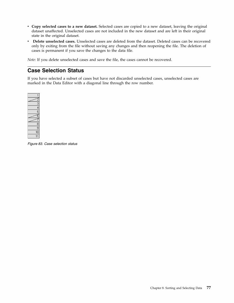
v Copy selected cases to a new dataset. Selected cases are copied to a new dataset, leaving the originaldataset unaffected. Unselected cases are not included in the new dataset and are left in their originalstate in the original dataset.

v Delete unselected cases. Unselected cases are deleted from the dataset. Deleted cases can be recoveredonly by exiting from the file without saving any changes and then reopening the file. The deletion ofcases is permanent if you save the changes to the data file.

Note: If you delete unselected cases and save the file, the cases cannot be recovered.

Case Selection StatusIf you have selected a subset of cases but have not discarded unselected cases, unselected cases aremarked in the Data Editor with a diagonal line through the row number.

Figure 83. Case selection status


Chapter 9. Sample Files

The sample files installed with the product can be found in the Samples subdirectory of the installationdirectory. There is a separate folder within the Samples subdirectory for each of the following languages:English, French, German, Italian, Japanese, Korean, Polish, Russian, Simplified Chinese, Spanish, andTraditional Chinese.

Not all sample files are available in all languages. If a sample file is not available in a language, thatlanguage folder contains an English version of the sample file.

Descriptions

Following are brief descriptions of the sample files used in various examples throughout thedocumentation. For the Student Version, some data files are subsets of the original data files because theStudent Version has a limit of 1,500 cases.v accidents.sav. This is a hypothetical data file that concerns an insurance company that is studying age

and gender risk factors for automobile accidents in a given region. Each case corresponds to across-classification of age category and gender.

v adl.sav. This is a hypothetical data file that concerns efforts to determine the benefits of a proposedtype of therapy for stroke patients. Physicians randomly assigned female stroke patients to one of twogroups. The first received the standard physical therapy, and the second received an additionalemotional therapy. Three months following the treatments, each patient's abilities to perform commonactivities of daily life were scored as ordinal variables.

v advert.sav. This is a hypothetical data file that concerns a retailer's efforts to examine the relationshipbetween money spent on advertising and the resulting sales. To this end, they have collected past salesfigures and the associated advertising costs.

v aflatoxin.sav. This is a hypothetical data file that concerns the testing of corn crops for aflatoxin, apoison whose concentration varies widely between and within crop yields. A grain processor hasreceived 16 samples from each of 8 crop yields and measured the alfatoxin levels in parts per billion(PPB).

v anticonvulsants.sav. Medical researchers can use a generalized linear mixed model to determinewhether a new anticonvulsant drug can reduce a patient's rate of epileptic seizures. Repeatedmeasurements from the same patient are typically positively correlated so a mixed model with somerandom effects should be appropriate. The target field, the number of seizures, takes positive integervalues, so a generalized linear mixed model with a Poisson distribution and log link may beappropriate.

v bankloan.sav. This is a hypothetical data file that concerns a bank's efforts to reduce the rate of loandefaults. The file contains financial and demographic information on 850 past and prospectivecustomers. The first 700 cases are customers who were previously given loans. The last 150 cases areprospective customers that the bank needs to classify as good or bad credit risks.

v bankloan_cs.sav. This is a hypothetical data file that concerns a bank's efforts to identify characteristicsthat are indicative of people who are likely to default on loans and then use those characteristics toidentify good and bad credit risks.

v bankloan_cs_noweights.sav. This is a hypothetical data file that concerns a bank's efforts to identifycharacteristics that are indicative of people who are likely to default on loans and then use thosecharacteristics to identify good and bad credit risks. The sampling weights are not included in the file.

v brakes.sav. This is a hypothetical data file that concerns quality control at a factory that produces discbrakes for high-performance automobiles. The data file contains diameter measurements of 16 discsfrom each of 8 production machines. The target diameter for the brakes is 322 millimeters.

79

v cable_survey.sav. Executives at a cable provider of television, phone, and internet services want toknow more about potential customers. They conduct a survey of 2000 people in their service regionsand ask whether they (1) don't have the service; (2) subscribe to the service with other providers; or (3)have the service with the company, for each of the three services. The survey additionally collects somedemographic information, such as gender, age category (4 levels), education category (3 levels), incomecategory (3 levels), residence type category (4 levels), years at current address category (3 levels),number of people in the house, and so on.

v car_sales.sav. This data file contains hypothetical sales estimates, list prices, and physical specificationsfor various makes and models of vehicles. The list prices and physical specifications were obtainedalternately from edmunds.com and manufacturer sites.

v car_sales_uprepared.sav. This is a modified version of car_sales.sav that does not include anytransformed versions of the fields.

v cellular.sav. This is a hypothetical data file that concerns a cellular phone company's efforts to reducechurn. Churn propensity scores are applied to accounts, ranging from 0 to 100. Accounts scoring 50 orabove may be looking to change providers.

v ceramics.sav. This is a hypothetical data file that concerns a manufacturer's efforts to determinewhether a new premium alloy has a greater heat resistance than a standard alloy. Each case representsa separate test of one of the alloys; the heat at which the bearing failed is recorded.

v clothing_defects.sav. This is a hypothetical data file that concerns the quality control process at aclothing factory. From each lot produced at the factory, the inspectors take a sample of clothes andcount the number of clothes that are unacceptable.

v credit_card.sav. A hypothetical study of credit card usage follows each subject's monthly spending ontheir primary card for two years, with spending broken out by the type of transaction (Grocery, Retail,Entertainment, Travel, and Other). Each record in the dataset corresponds to given month of spendingand type of transaction, so the data collected for each subject requires 2 years × 12 months per year × 5types of transactions = 120 records.

v creditpromo.sav. This is a hypothetical data file that concerns a department store's efforts to evaluatethe effectiveness of a recent credit card promotion. To this end, 500 cardholders were randomlyselected. Half received an ad promoting a reduced interest rate on purchases made over the next threemonths. Half received a standard seasonal ad.

v cross_sell.sav. An order-by-mail company has a book club and a CD club. Each month, they makespecial offers available to club members. The company wants to create a model for the month's totalspecial offer purchases based on total book purchases, CD purchases, and the type of offer given toclub members. Two-Stage Least-Squares Regression is appropriate to this situation because moneyspent on special offers is money not spent on books or CD's; thus, there is a feedback loop between theresponse and these two predictors.

v demo.sav. This is a hypothetical data file that concerns a purchased customer database, for the purposeof mailing monthly offers. Whether or not the customer responded to the offer is recorded, along withvarious demographic information. For the Student Version, this is a sample of 1,000 cases from thelarger original file.

v dietstudy.sav. This hypothetical data file contains the results of a study of the "Stillman diet" 1. Eachcase corresponds to a separate subject and records his or her pre- and post-diet weights in pounds andtriglyceride levels in mg/100 ml.

v dvdplayer.sav. This is a hypothetical data file that concerns the development of a new DVD player.Using a prototype, the marketing team has collected focus group data. Each case corresponds to aseparate surveyed user and records some demographic information about them and their responses toquestions about the prototype.

v Employee data.sav. This is a hypothetical data file that contains employee specific information(education level, employment category, current salary, previous experience, and so on).

1. Rickman, R., N. Mitchell, J. Dingman, and J. E. Dalen. 1974. Changes in serum cholesterol during the Stillman Diet. Journal of theAmerican Medical Association, 228:, 54-58.


v german_credit.sav. This data file is taken from the "German credit" dataset in the Repository ofMachine Learning Databases 2 at the University of California, Irvine.

v grocery_1month.sav. This hypothetical data file is the grocery_coupons.sav data file with the weeklypurchases "rolled-up" so that each case corresponds to a separate customer. Some of the variables thatchanged weekly disappear as a result, and the amount spent recorded is now the sum of the amountsspent during the four weeks of the study.

v health_funding.sav. This is a hypothetical data file that contains data on health care funding (amountper 100 population), disease rates (rate per 10,000 population), and visits to health care providers (rateper 10,000 population). Each case represents a different city.

v hivassay.sav. This is a hypothetical data file that concerns the efforts of a pharmaceutical lab to developa rapid assay for detecting HIV infection. The results of the assay are eight deepening shades of red,with deeper shades indicating greater likelihood of infection. A laboratory trial was conducted on 2,000blood samples, half of which were infected with HIV and half of which were clean. For the StudentVersion, this is a sample of 1,000 cases from the larger original file.

v hourlywagedata.sav. This is a hypothetical data file that concerns the hourly wages of nurses fromoffice and hospital positions and with varying levels of experience. For the Student Version, this is asample of 1,000 cases from the larger original file.

v insurance_claims.sav. This is a hypothetical data file that concerns an insurance company that wants tobuild a model for flagging suspicious, potentially fraudulent claims. Each case represents a separateclaim.

v judges.sav. This is a hypothetical data file that concerns the scores given by trained judges (plus oneenthusiast) to 300 gymnastics performances. Each row represents a separate performance; the judgesviewed the same performances.

v marketvalues.sav. This data file concerns home sales in a new housing development in Algonquin, Ill.,during the years from 1999–2000. These sales are a matter of public record.

v property_assess.sav. This is a hypothetical data file that concerns a county assessor's efforts to keepproperty value assessments up to date on limited resources. The cases correspond to properties sold inthe county in the past year. Each case in the data file records the township in which the property lies,the assessor who last visited the property, the time since that assessment, the valuation made at thattime, and the sale value of the property.

v salesperformance.sav. This is a hypothetical data file that concerns the evaluation of two new salestraining courses. Sixty employees, divided into three groups, all receive standard training. In addition,group 2 gets technical training; group 3, a hands-on tutorial. Each employee was tested at the end ofthe training course and their score recorded. Each case in the data file represents a separate trainee andrecords the group to which they were assigned and the score they received on the exam.

v satisf.sav. This is a hypothetical data file that concerns a satisfaction survey conducted by a retailcompany at 4 store locations. 582 customers were surveyed in all, and each case represents theresponses from a single customer.

v shampoo_ph.sav. This is a hypothetical data file that concerns the quality control at a factory for hairproducts. At regular time intervals, six separate output batches are measured and their pH recorded.The target range is 4.5–5.5.

v site.sav. This is a hypothetical data file that concerns a company's efforts to choose new sites for theirexpanding business. They have hired two consultants to separately evaluate the sites, who, in additionto an extended report, summarized each site as a "good," "fair," or "poor" prospect.

v smokers.sav. This data file is abstracted from the 1998 National Household Survey of Drug Abuse andis a probability sample of American households. (http://dx.doi.org/10.3886/ICPSR02934) Thus, thefirst step in an analysis of this data file should be to weight the data to reflect population trends. Forthe Student Version, this is a sample of 1,000 cases from the larger original file.

2. Blake, C. L., and C. J. Merz. 1998. "UCI Repository of machine learning databases." Available at http://www.ics.uci.edu/~mlearn/MLRepository.html.

Chapter 9. Sample Files 81

http://dx.doi.org/10.3886/ICPSR02934

http://www.ics.uci.edu/~mlearn/MLRepository.html

http://www.ics.uci.edu/~mlearn/MLRepository.html

v tcm_kpi.sav. This is a hypothetical data file that contains values of weekly key performance indicatorsfor a business. It also contains weekly data for a number of controllable metrics over the same timeperiod.

v tcm_kpi_upd.sav. This data file is identical to tcm_kpi.sav but contains data for four extra weeks.v telco.sav. This is a hypothetical data file that concerns a telecommunications company's efforts to

reduce churn in their customer base. Each case corresponds to a separate customer and records variousdemographic and service usage information.

v telco_extra.sav. This data file is similar to the telco.sav data file, but the "tenure" and log-transformedcustomer spending variables have been removed and replaced by standardized log-transformedcustomer spending variables.

v tv-survey.sav. This is a hypothetical data file that concerns a survey conducted by a TV studio that isconsidering whether to extend the run of a successful program. 906 respondents were asked whetherthey would watch the program under various conditions. Each row represents a separate respondent;each column is a separate condition.

v virus.sav. This is a hypothetical data file that concerns the efforts of an Internet service provider (ISP)to determine the effects of a virus on its networks. They have tracked the (approximate) percentage ofinfected e-mail traffic on its networks over time, from the moment of discovery until the threat wascontained.

v workprog.sav. This is a hypothetical data file that concerns a government works program that tries toplace disadvantaged people into better jobs. A sample of potential program participants were followed,some of whom were randomly selected for enrollment in the program, while others were not. Eachcase represents a separate program participant.

v worldsales.sav This hypothetical data file contains sales revenue by continent and product.


Notices

This information was developed for products and services offered in the US. This material might beavailable from IBM in other languages. However, you may be required to own a copy of the product orproduct version in that language in order to access it.

IBM may not offer the products, services, or features discussed in this document in other countries.Consult your local IBM representative for information on the products and services currently available inyour area. Any reference to an IBM product, program, or service is not intended to state or imply thatonly that IBM product, program, or service may be used. Any functionally equivalent product, program,or service that does not infringe any IBM intellectual property right may be used instead. However, it isthe user's responsibility to evaluate and verify the operation of any non-IBM product, program, orservice.

IBM may have patents or pending patent applications covering subject matter described in thisdocument. The furnishing of this document does not grant you any license to these patents. You can sendlicense inquiries, in writing, to:

IBM Director of LicensingIBM CorporationNorth Castle Drive, MD-NC119Armonk, NY 10504-1785US

For license inquiries regarding double-byte (DBCS) information, contact the IBM Intellectual PropertyDepartment in your country or send inquiries, in writing, to:

Intellectual Property LicensingLegal and Intellectual Property LawIBM Japan Ltd.19-21, Nihonbashi-Hakozakicho, Chuo-kuTokyo 103-8510, Japan

INTERNATIONAL BUSINESS MACHINES CORPORATION PROVIDES THIS PUBLICATION "AS IS"WITHOUT WARRANTY OF ANY KIND, EITHER EXPRESS OR IMPLIED, INCLUDING, BUT NOTLIMITED TO, THE IMPLIED WARRANTIES OF NON-INFRINGEMENT, MERCHANTABILITY ORFITNESS FOR A PARTICULAR PURPOSE. Some jurisdictions do not allow disclaimer of express orimplied warranties in certain transactions, therefore, this statement may not apply to you.

This information could include technical inaccuracies or typographical errors. Changes are periodicallymade to the information herein; these changes will be incorporated in new editions of the publication.IBM may make improvements and/or changes in the product(s) and/or the program(s) described in thispublication at any time without notice.

Any references in this information to non-IBM websites are provided for convenience only and do not inany manner serve as an endorsement of those websites. The materials at those websites are not part ofthe materials for this IBM product and use of those websites is at your own risk.

IBM may use or distribute any of the information you provide in any way it believes appropriate withoutincurring any obligation to you.

83

Licensees of this program who wish to have information about it for the purpose of enabling: (i) the exchange of information between independently created programs and other programs (including this one) and (ii) the mutual use of the information which has been exchanged, should contact:

IBM Director of LicensingIBM CorporationNorth Castle Drive, MD-NC119Armonk, NY 10504-1785US

Such information may be available, subject to appropriate terms and conditions, including in some cases, payment of a fee.

The licensed program described in this document and all licensed material available for it are provided by IBM under terms of the IBM Customer Agreement, IBM International Program License Agreement or any equivalent agreement between us.

The performance data and client examples cited are presented for illustrative purposes only. Actual performance results may vary depending on specific configurations and operating conditions.

Information concerning non-IBM products was obtained from the suppliers of those products, their published announcements or other publicly available sources. IBM has not tested those products and cannot confirm the accuracy of performance, compatibility or any other claims related tonon-IBMproducts. Questions on the capabilities of non-IBM products should be addressed to the suppliers of those products.

Statements regarding IBM's future direction or intent are subject to change or withdrawal without notice, and represent goals and objectives only.

This information contains examples of data and reports used in daily business operations. To illustrate them as completely as possible, the examples include the names of individuals, companies, brands, and products. All of these names are fictitious and any similarity to actual people or business enterprises is entirely coincidental.

COPYRIGHT LICENSE:

This information contains sample application programs in source language, which illustrate programming techniques on various operating platforms. You may copy, modify, and distribute these sample programs in any form without payment to IBM, for the purposes of developing, using, marketing or distributing application programs conforming to the application programming interface for the operating platform for which the sample programs are written. These examples have not been thoroughly tested under all conditions. IBM, therefore, cannot guarantee or imply reliability, serviceability, or function of these programs. The sample programs are provided "AS IS", without warranty of any kind. IBM shall not be liable for any damages arising out of your use of the sample programs.

Each copy or any portion of these sample programs or any derivative work, must include a copyright notice as follows:

© IBM 2019. Portions of this code are derived from IBM Corp. Sample Programs.

© Copyright IBM Corp. 1989 - 2019. All rights reserved.


TrademarksIBM, the IBM logo, and ibm.com are trademarks or registered trademarks of International BusinessMachines Corp., registered in many jurisdictions worldwide. Other product and service names might betrademarks of IBM or other companies. A current list of IBM trademarks is available on the web at"Copyright and trademark information" at www.ibm.com/legal/copytrade.shtml.

Adobe, the Adobe logo, PostScript, and the PostScript logo are either registered trademarks or trademarksof Adobe Systems Incorporated in the United States, and/or other countries.

Intel, Intel logo, Intel Inside, Intel Inside logo, Intel Centrino, Intel Centrino logo, Celeron, Intel Xeon,Intel SpeedStep, Itanium, and Pentium are trademarks or registered trademarks of Intel Corporation or itssubsidiaries in the United States and other countries.

Linux is a registered trademark of Linus Torvalds in the United States, other countries, or both.

Microsoft, Windows, Windows NT, and the Windows logo are trademarks of Microsoft Corporation in theUnited States, other countries, or both.

UNIX is a registered trademark of The Open Group in the United States and other countries.

Java and all Java-based trademarks and logos are trademarks or registered trademarks of Oracle and/orits affiliates.

Notices 85

http://www.ibm.com/legal/us/en/copytrade.shtml

Index

AAccess (Microsoft) 11

Bbar charts 28

Ccases

selecting 73sorting 71, 73

categorical data 27summary measures 27

chartsbar 28, 33creating charts 33histograms 30

computing new variables 65conditional expressions 67continuous data 27counts

tables of counts 27create variable labels 21

DData Editor

entering non-numeric data 20entering numeric data 19

data entry 19, 20data types

for variables 22database files

reading 11Database Wizard 11date and time variables 68Date and Time Wizard 68

Eediting pivot tables 43entering data

non-numeric 20numeric 19

Excel (Microsoft)exporting results to 53

Excel filesreading 8

exporting resultsHTML 60to Excel 53to PowerPoint 53to Word 53

Ffrequency tables 27functions in expressions 66

Ggraphs

bar 33creating graphs 33

Hhiding rows and columns in pivot

tables 44histograms 30HTML

exporting results 60

Iinterval data 27

Llayers

creating in pivot tables 42level of measurement 27

Mmeasurement level 27missing values

for non-numeric variables 24for numeric variables 24system-missing 23

movingelements in pivot tables 41items in the Viewer 39

Nnominal data 27numeric data 19

Oordinal data 27

Ppivot tables

accessing definitions 40cell data types 44cell formats 44editing 43formatting 43hiding decimal points 44

pivot tables (continued)hiding rows and columns 44layers 42pivoting trays 41transposing rows and columns 41

PowerPoint (Microsoft)exporting results to 53

Qqualitative data 27quantitative data 27

Rratio data 27recoding values 63

Ssample files

location 79scale data 27scale variables

summary measures 29selecting cases 73sorting cases 71split-file processing 71spreadsheet files

reading 8reading variable names 8

string dataentering data 20

subsets of casesbased on dates and times 76conditional expressions 74deleting unselected cases 76filtering unselected cases 76if condition is satisfied 74random sample 75selecting 73

summary measurescategorical data 27scale variables 29

system-missing values 23

Ttext data files

reading 14Text Import Wizard 14transposing (flipping) rows and columns

in pivot tables 41

Vvalue labels

assigning 23controlling display in Viewer 23

87

value labels (continued)numeric variables 23

variable labelscreating 21

variables 19data types 22labels 21

Viewerhiding and showing output 39moving output 39

WWord (Microsoft)

exporting results to 53


IBM®

Printed in USA

IBM SPSS Statistics 25 Brief Guide - KendallHunt · 2 IBM SPSS Statistics 26 Brief Guide Running an...

Documents

Transcript of IBM SPSS Statistics 25 Brief Guide - KendallHunt · 2 IBM SPSS Statistics 26 Brief Guide Running an...