Hydrogeology and Ground-Water Flow in the Edwards-Trinity ... · Hydrogeology and Ground-Water Flow...
85
Hydrogeology and Ground-Water Flow in the Edwards-Trinity Aquifer System, West-Central Texas Regional Aquifer-System Analysis—Edwards-Trinity By Eve L. Kuniansky and Ann F. Ardis U.S. Department of the Interior U.S. Geological Survey Professional Paper 1421-C
-
Upload
vuongthuan -
Category
Documents
-
view
226 -
download
6
Transcript of Hydrogeology and Ground-Water Flow in the Edwards-Trinity ... · Hydrogeology and Ground-Water Flow...
Hydrogeology and Ground-Water Flow in the Edwards-Trinity Aquifer System,West-Central Texas
Regional Aquifer-System Analysis—Edwards-Trinity
By Eve L. Kuniansky and Ann F. Ardis
U.S. Department of the InteriorU.S. Geological Survey
Professional Paper 1421-C
U.S. Department of the InteriorGale A. Norton, Secretary
U.S. Geological SurveyCharles G. Groat, Director
U.S. Geological Survey, Reston, Virginia: 2004For sale by U.S. Geological Survey, Information ServicesBox 25286, Denver Federal CenterDenver, CO 80225
For more information about the USGS and its products:Telephone: 1-888-ASK-USGSWorld Wide Web: http://www.usgs.gov/
Any use of trade, product, or firm names in this publication is for descriptive purposes only and does not imply endorsement by the U.S. Government.
Although this report is in the public domain, permission must be secured from the individual copyright owners to repro-duce any copyrighted materials contained within this report.
ISBN
Suggested citation:Kuniansky, Eve L., and Ardis, Ann F., 2004, Hydrogeology and ground-water flow in the Edwards-Trinity aquifer system,
west-central Texas: Regional aquifer-system analysis—Edwards-Trinity: U.S. Geological Survey Professional Paper1421-C, p. .
Library of Congress Cataloging-in-Publication Data
Kuniansky, Eve L.Hydrogeology and ground-water flow in the Edwards-Trinity aquifer system, west-central Texas by Eve L Kuniansky and
Ann F. Ardisp. cm. —(Regional aquifer-system analysis—Edwards-Trinity aquifer system) (U.S. Geological Survey professional
paper; 1421-C)Includes bibliographical references.Supt. of Docs. no.:1. Edwards-Trinity Aquifer (Tex.) 2. Edwards Aquifer (Tex.) 3. Trinity Aquifer (Tex.) 4. Water, Underground-TexasI. Title II. Series. III. Series: U.S. Geological Survey professional paper 1421-C
CIP
iii
FOREWORD
THE REGIONAL AQUIFER-SYSTEM ANALYSIS PROGRAM
The RASA Program represents a systematic effort to study a number of the Nation’s most important aquifer systems, which, in aggregate, underlie much of the country and which represent an important component of the Nation’s total water supply. In general, the boundaries of these studies are identified by the hydrologic extent of each system and, accordingly, transcend the political subdivisions to which investigations have often arbitrarily been limited in the past. The broad objective for each study is to assemble geologic, hydrologic, and geochemical information, to analyze and develop an understanding of the system, and to develop predictive capability that will contribute to the effective management of the system. The use of computer simulation is an important element of the RASA studies to develop an understanding of the natural, undisturbed hydrologic system and the changes brought about in it by human activities and to provide a means of predicting the regional effects of future pumping or other stresses.
The final interpretive results of the RASA Program are presented in a series of U.S. Geological Survey Professional Papers that describe the geology, hydrology, and geochemistry of each regional aquifer. Each study within the RASA Program is assigned a single Professional Paper number beginning with Professional Paper 1400.
Charles G. GroatDirector

v
Contents
Abstract . . . . . . . . . . . . . . . . . . . . . . . . . . . . . . . . . . . . . . . . . . . . . . . . . . . . . . . . . . . . . . . . . . . . . . . . . . . . .1Introduction . . . . . . . . . . . . . . . . . . . . . . . . . . . . . . . . . . . . . . . . . . . . . . . . . . . . . . . . . . . . . . . . . . . . . . . . . .3
Purpose and Scope . . . . . . . . . . . . . . . . . . . . . . . . . . . . . . . . . . . . . . . . . . . . . . . . . . . . . . . . . . . . . . . . . . . . . . . . . . . . . . . . . . . 3Previous Studies . . . . . . . . . . . . . . . . . . . . . . . . . . . . . . . . . . . . . . . . . . . . . . . . . . . . . . . . . . . . . . . . . . . . . . . . . . . . . . . . . . . . . . 5Physiography and Hydrologic Setting. . . . . . . . . . . . . . . . . . . . . . . . . . . . . . . . . . . . . . . . . . . . . . . . . . . . . . . . . . . . . . . . . . 6
Hydrogeology. . . . . . . . . . . . . . . . . . . . . . . . . . . . . . . . . . . . . . . . . . . . . . . . . . . . . . . . . . . . . . . . . . . . . . . .10Edwards–Trinity Aquifer System and Contiguous Hydraulically Connected Units . . . . . . . . . . . . . . . . . . . . . . 10Structural Controls on Ground-Water Flow . . . . . . . . . . . . . . . . . . . . . . . . . . . . . . . . . . . . . . . . . . . . . . . . . . . . . . . . . . . 15Hydraulic Characteristics. . . . . . . . . . . . . . . . . . . . . . . . . . . . . . . . . . . . . . . . . . . . . . . . . . . . . . . . . . . . . . . . . . . . . . . . . . . . . 16
Transmissivity. . . . . . . . . . . . . . . . . . . . . . . . . . . . . . . . . . . . . . . . . . . . . . . . . . . . . . . . . . . . . . . . . . . . . . . . . . . . . . . . . . . 16Anisotropy. . . . . . . . . . . . . . . . . . . . . . . . . . . . . . . . . . . . . . . . . . . . . . . . . . . . . . . . . . . . . . . . . . . . . . . . . . . . . . . . . . . . . . 19Vertical Hydraulic Conductivity. . . . . . . . . . . . . . . . . . . . . . . . . . . . . . . . . . . . . . . . . . . . . . . . . . . . . . . . . . . . . . . . . . 19Storage Coefficient . . . . . . . . . . . . . . . . . . . . . . . . . . . . . . . . . . . . . . . . . . . . . . . . . . . . . . . . . . . . . . . . . . . . . . . . . . . . . 19
Ground-Water Use. . . . . . . . . . . . . . . . . . . . . . . . . . . . . . . . . . . . . . . . . . . . . . . . . . . . . . . . . . . . . . . . . . . . . . . . . . . . . . . . . . . 20Long-Term Water-Level Variations. . . . . . . . . . . . . . . . . . . . . . . . . . . . . . . . . . . . . . . . . . . . . . . . . . . . . . . . . . . . . . . . . . . . 28Potentiometric Surface. . . . . . . . . . . . . . . . . . . . . . . . . . . . . . . . . . . . . . . . . . . . . . . . . . . . . . . . . . . . . . . . . . . . . . . . . . . . . . . 29Natural Recharge and Discharge. . . . . . . . . . . . . . . . . . . . . . . . . . . . . . . . . . . . . . . . . . . . . . . . . . . . . . . . . . . . . . . . . . . . . 34
Ground-Water Flow . . . . . . . . . . . . . . . . . . . . . . . . . . . . . . . . . . . . . . . . . . . . . . . . . . . . . . . . . . . . . . . . . .38Regional Steady-State Simulations of Ground-Water Flow. . . . . . . . . . . . . . . . . . . . . . . . . . . . . . . . . . . . . . . . . . . . 40
Regional Model Development . . . . . . . . . . . . . . . . . . . . . . . . . . . . . . . . . . . . . . . . . . . . . . . . . . . . . . . . . . . . . . . . . . 40Finite-Element Method . . . . . . . . . . . . . . . . . . . . . . . . . . . . . . . . . . . . . . . . . . . . . . . . . . . . . . . . . . . . . . . . . . . . 41Regional Finite-Element Mesh and Lateral Boundaries . . . . . . . . . . . . . . . . . . . . . . . . . . . . . . . . . . . . 41Internal Boundaries. . . . . . . . . . . . . . . . . . . . . . . . . . . . . . . . . . . . . . . . . . . . . . . . . . . . . . . . . . . . . . . . . . . . . . . 41Water Budgets from Steady-State Regional Simulations. . . . . . . . . . . . . . . . . . . . . . . . . . . . . . . . . . . 41Direction of Ground-Water Movement . . . . . . . . . . . . . . . . . . . . . . . . . . . . . . . . . . . . . . . . . . . . . . . . . . . . 46
Subregional Transient Simulations of Ground-Water Flow in the Edwards and Trinity Aquifers . . . . . . . . 46Subregional Model Development . . . . . . . . . . . . . . . . . . . . . . . . . . . . . . . . . . . . . . . . . . . . . . . . . . . . . . . . . . . . . . . 46
Subregional Finite-Element Mesh, Lateral and Internal Boundaries. . . . . . . . . . . . . . . . . . . . . . . . 47Model Layering . . . . . . . . . . . . . . . . . . . . . . . . . . . . . . . . . . . . . . . . . . . . . . . . . . . . . . . . . . . . . . . . . . . . . . . . . . . 47
Transient Simulations of Recent Conditions (1978–89) . . . . . . . . . . . . . . . . . . . . . . . . . . . . . . . . . . . . . . . . . . . 48Water Budget from Transient Simulation . . . . . . . . . . . . . . . . . . . . . . . . . . . . . . . . . . . . . . . . . . . . . . . . . . 53Direction of Ground-Water Movement and Description of Flow Paths . . . . . . . . . . . . . . . . . . . . . 56Limitations of the Subregional Model and Flow Path Analysis. . . . . . . . . . . . . . . . . . . . . . . . . . . . . . 60
Summary and Conclusions . . . . . . . . . . . . . . . . . . . . . . . . . . . . . . . . . . . . . . . . . . . . . . . . . . . . . . . . . . . .61Selected References . . . . . . . . . . . . . . . . . . . . . . . . . . . . . . . . . . . . . . . . . . . . . . . . . . . . . . . . . . . . . . . . .62Initial Conditions . . . . . . . . . . . . . . . . . . . . . . . . . . . . . . . . . . . . . . . . . . . . . . . . . . . . . . . . . . . . . . . . . . . . .72Time-Step Size. . . . . . . . . . . . . . . . . . . . . . . . . . . . . . . . . . . . . . . . . . . . . . . . . . . . . . . . . . . . . . . . . . . . . . .72Calibration . . . . . . . . . . . . . . . . . . . . . . . . . . . . . . . . . . . . . . . . . . . . . . . . . . . . . . . . . . . . . . . . . . . . . . . . . .72Sensitivity Analysis . . . . . . . . . . . . . . . . . . . . . . . . . . . . . . . . . . . . . . . . . . . . . . . . . . . . . . . . . . . . . . . . . . .74
vi Edwards–Trinity Aquifer System, West-Central Texas
Plates
[In pocket]1. Regional model and finite-element mesh2. Subregional model and finite-element mesh and layering3. Regional potentiometric surface, magnitude and direction of flow4. Subregional potentiometric surface, magnitude and direction of flow
Figures
1–2. Maps showing—1. Study area and major and minor aquifers, west-central Texas . . . . . . . . . . . . . . . . . . . . . . . . . . . . . . . 42. Faults associated with the Balcones fault zone, central Texas. . . . . . . . . . . . . . . . . . . . . . . . . . . . . . . . 8
3. Graphs showing mean monthly precipitation and pan evaporation at selected locations, west-central Texas. . . . . . . . . . . . . . . . . . . . . . . . . . . . . . . . . . . . . . . . . . . . . . . . . . . . . . . . . . . . . . . . . . . . . . . . . . . . . . . .9
4. Correlation chart showing hydrogeologic units, major aquifers, and their stratigraphic equivalents, west-central Texas . . . . . . . . . . . . . . . . . . . . . . . . . . . . . . . . . . . . . . . . . . . . . . . . . . . . . . . . . . . . . . . . . .11
5. Diagram showing generalized section showing the geologic or hydrogeologic units simulatedas one layer in the regional model, west-central Texas. . . . . . . . . . . . . . . . . . . . . . . . . . . . . . . . . . . . . . . . . . . .13
6–10. Maps showing—6. Estimated transmissivity of the Edwards–Trinity aquifer system and contiguous,
hydraulically connected units from the regional model, west-central Texas . . . . . . . . . . . . . . . . . 177. Estimated transmissivity of the Edwards and Trinity aquifers from the subregional
model, central Texas. . . . . . . . . . . . . . . . . . . . . . . . . . . . . . . . . . . . . . . . . . . . . . . . . . . . . . . . . . . . . . . . . . . . . . . . 188. Estimated distribution of anisotropy in the Edwards and Trinity aquifers from the
subregional model, central Texas . . . . . . . . . . . . . . . . . . . . . . . . . . . . . . . . . . . . . . . . . . . . . . . . . . . . . . . . . . . 209. Estimated vertical leakage coefficients of confining units from the subregional model,
central Texas . . . . . . . . . . . . . . . . . . . . . . . . . . . . . . . . . . . . . . . . . . . . . . . . . . . . . . . . . . . . . . . . . . . . . . . . . . . . . . . 2110. Estimated storage coefficients from the subregional model, central Texas. . . . . . . . . . . . . . . . . . . 22
11. Map and graph showing summary of census and water-use data, by county by geographic subarea, west-central Texas . . . . . . . . . . . . . . . . . . . . . . . . . . . . . . . . . . . . . . . . . . . . . . . . . . . . . . . . . . . . . . . . . . . . .25
12. Graphs showing hydrologic data and pumpage for the San Antonio segment of the Edwards aquifer, central Texas . . . . . . . . . . . . . . . . . . . . . . . . . . . . . . . . . . . . . . . . . . . . . . . . . . . . . . . . . . . . . . . . . . . . . . . . . . . .26
13. Map with pie charts showing estimated ground-water withdrawals, by county, west-central Texas, 1990. . . . . . . . . . . . . . . . . . . . . . . . . . . . . . . . . . . . . . . . . . . . . . . . . . . . . . . . . . . . . . . . . . . . . . . . . . . . . . . . . . . . . . .27
14. Graphs showing selected hydrographs showing long-term water-level variations, west-central Texas. . . . . . . . . . . . . . . . . . . . . . . . . . . . . . . . . . . . . . . . . . . . . . . . . . . . . . . . . . . . . . . . . . . . . . . . . . . . . . .30
15–16. Maps showing—15. Simulated and observed predevelopment potentiometric surfaces of the Edwards–
Trinity aquifer system and contiguous, hydraulically connected units, west-central Texas . . . 3216. Simulated and observed postdevelopment potentiometric surfaces of the Edwards–
Trinity aquifer system and contiguous, hydraulically connected units, west-central Texas, winter 1974–75. . . . . . . . . . . . . . . . . . . . . . . . . . . . . . . . . . . . . . . . . . . . . . . . . . . . . . . . . . . . . . . . . . . . . . . 33
17. Estimated recharge from regional model simulations, west-central Texas. . . . . . . . . . . . . . . . . . . 3518. Hydrograph showing historical monthly springflow discharge at Comal, San Marcos, and
Barton Springs, central Texas . . . . . . . . . . . . . . . . . . . . . . . . . . . . . . . . . . . . . . . . . . . . . . . . . . . . . . . . . . . . . . . . . . . .3919–20. Diagrams showing water budget components for major aquifers of the Edwards–Trinity
aquifer system and contiguous units, west-central Texas19. Predevelopment . . . . . . . . . . . . . . . . . . . . . . . . . . . . . . . . . . . . . . . . . . . . . . . . . . . . . . . . . . . . . . . . . . . . . . . . . . . .4320 Winter 1974–75 . . . . . . . . . . . . . . . . . . . . . . . . . . . . . . . . . . . . . . . . . . . . . . . . . . . . . . . . . . . . . . . . . . . . . . . . . . . . . 44
Tables vii
21–22. Maps showing—21. Potentiometric-surface contours of source or sink layers used in the subregional model,
central Texas. . . . . . . . . . . . . . . . . . . . . . . . . . . . . . . . . . . . . . . . . . . . . . . . . . . . . . . . . . . . . . . . . . . . . . . . . . . . . . . 4922. Simulated potentiometric-surface contours of the lower Trinity aquifer used a specified
head in the subregional model transient simulation, central Texas . . . . . . . . . . . . . . . . . . . . . . . . . . 5023–25. Hydrographs showing—
23. Observed and simulated springflow at major springs in the subregional model, central Texas, 1978–89 . . . . . . . . . . . . . . . . . . . . . . . . . . . . . . . . . . . . . . . . . . . . . . . . . . . . . . . . . . . . . . . . . . . . . . . . . . . . . 51
24. Simulated springflow at minor springs in the subregional model, central Texas, 1978–89 . . . . 5225. Observed and simulated water levels at selected observation wells in the Edwards aquifer,
central Texas, 1978-89 . . . . . . . . . . . . . . . . . . . . . . . . . . . . . . . . . . . . . . . . . . . . . . . . . . . . . . . . . . . . . . . . . . . . . . 5426. Schematic diagram showing water budget components computed form average simulated
water levels of the subregional model, central Texas, 1978–89. . . . . . . . . . . . . . . . . . . . . . . . . . . . . . . . . . . . 5627. Hydrograph showing simulated discharge from the aquifers (top model layer) to streams
and seeps in the Hill Country and Edwards Plateau, and the Balcones fault zone, central Texas . . 5728. Map showing selected flow paths from the subregional model, central Texas . . . . . . . . . . . . . . . . . . . . 59
29–34. Hydrographs showing sensitivity of the model to changes in 29. Transmissivity, 1978–80. . . . . . . . . . . . . . . . . . . . . . . . . . . . . . . . . . . . . . . . . . . . . . . . . . . . . . . . . . . . . . . . . . . . . 7530. Anisotropy, 1978–80 . . . . . . . . . . . . . . . . . . . . . . . . . . . . . . . . . . . . . . . . . . . . . . . . . . . . . . . . . . . . . . . . . . . . . . . . 7631. Angle of anisotropy, 1978–80. . . . . . . . . . . . . . . . . . . . . . . . . . . . . . . . . . . . . . . . . . . . . . . . . . . . . . . . . . . . . . . . 7732. Storage coefficient, 1978–80. . . . . . . . . . . . . . . . . . . . . . . . . . . . . . . . . . . . . . . . . . . . . . . . . . . . . . . . . . . . . . . . 7733. Vertical leakage coefficient, 1978–80 . . . . . . . . . . . . . . . . . . . . . . . . . . . . . . . . . . . . . . . . . . . . . . . . . . . . . . . 7834. Areally distributed recharge on the outcrop of the Edwards Group, 1978–80. . . . . . . . . . . . . . . . . .78
Tables
1. Withdrawals from the Edwards–Trinity aquifer system and contiguous, hydraulically connected units, west-central Texas, 1990 . . . . . . . . . . . . . . . . . . . . . . . . . . . . . . . . . . . . . . . . . . . . . . . . . . . . . . . . . . . . . . . . . . . 24
2. Wells used to construct long-term hydrographs . . . . . . . . . . . . . . . . . . . . . . . . . . . . . . . . . . . . . . . . . . . . . . . . . . .293. Baseflow estimates for gages in the Hill Country and southeast Edwards Plateau. . . . . . . . . . . . . . . . . 374. Simulated and observed springflows for the regional model . . . . . . . . . . . . . . . . . . . . . . . . . . . . . . . . . . . . . . 455. Root mean square error at selected wells and springs for transient simulation, 1978–89. . . . . . . . . . . 566. Summary of flow path analysis for average simulated potentiometric surface, 1978–89 . . . . . . . . . . . 58
REGIONAL AQUIFER-SYSTEM ANALYSIS—EDWARDS–TRINITY
HYDROGEOLOGY AND GROUND-WATER FLOW IN THE EDWARDS–TRINITY AQUIFER SYSTEM,
WEST-CENTRAL TEXAS
By Eve L. Kuniansky and Ann F. Ardis
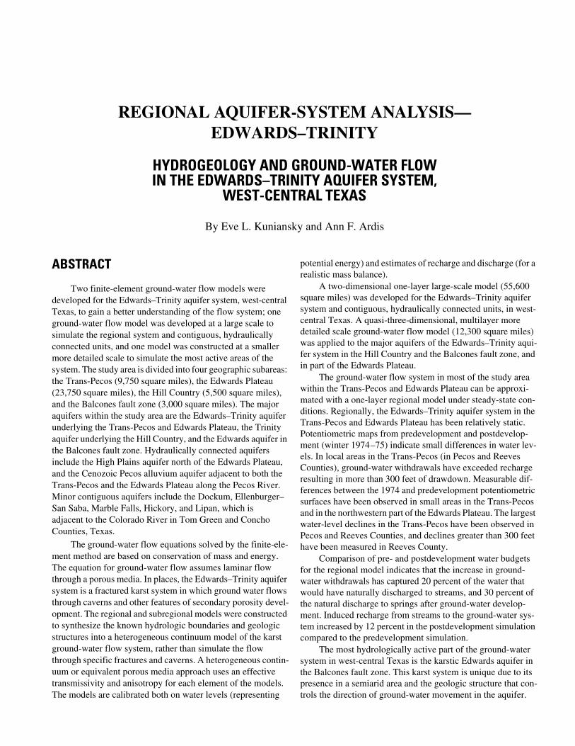
ABSTRACT
Two finite-element ground-water flow models were developed for the Edwards–Trinity aquifer system, west-central Texas, to gain a better understanding of the flow system; one ground-water flow model was developed at a large scale to simulate the regional system and contiguous, hydraulically connected units, and one model was constructed at a smaller more detailed scale to simulate the most active areas of the system. The study area is divided into four geographic subareas: the Trans-Pecos (9,750 square miles), the Edwards Plateau (23,750 square miles), the Hill Country (5,500 square miles), and the Balcones fault zone (3,000 square miles). The major aquifers within the study area are the Edwards–Trinity aquifer underlying the Trans-Pecos and Edwards Plateau, the Trinity aquifer underlying the Hill Country, and the Edwards aquifer in the Balcones fault zone. Hydraulically connected aquifers include the High Plains aquifer north of the Edwards Plateau, and the Cenozoic Pecos alluvium aquifer adjacent to both the Trans-Pecos and the Edwards Plateau along the Pecos River. Minor contiguous aquifers include the Dockum, Ellenburger–San Saba, Marble Falls, Hickory, and Lipan, which is adjacent to the Colorado River in Tom Green and Concho Counties, Texas.
The ground-water flow equations solved by the finite-ele-ment method are based on conservation of mass and energy. The equation for ground-water flow assumes laminar flow through a porous media. In places, the Edwards–Trinity aquifer system is a fractured karst system in which ground water flows through caverns and other features of secondary porosity devel-opment. The regional and subregional models were constructed to synthesize the known hydrologic boundaries and geologic structures into a heterogeneous continuum model of the karst ground-water flow system, rather than simulate the flow through specific fractures and caverns. A heterogeneous contin-uum or equivalent porous media approach uses an effective transmissivity and anisotropy for each element of the models. The models are calibrated both on water levels (representing
potential energy) and estimates of recharge and discharge (for a realistic mass balance).
A two-dimensional one-layer large-scale model (55,600 square miles) was developed for the Edwards–Trinity aquifer system and contiguous, hydraulically connected units, in west-central Texas. A quasi-three-dimensional, multilayer more detailed scale ground-water flow model (12,300 square miles) was applied to the major aquifers of the Edwards–Trinity aqui-fer system in the Hill Country and the Balcones fault zone, and in part of the Edwards Plateau.
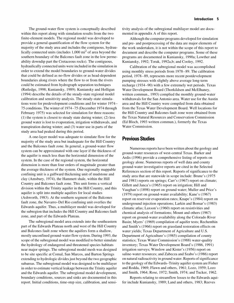
The ground-water flow system in most of the study area within the Trans-Pecos and Edwards Plateau can be approxi-mated with a one-layer regional model under steady-state con-ditions. Regionally, the Edwards–Trinity aquifer system in the Trans-Pecos and Edwards Plateau has been relatively static. Potentiometric maps from predevelopment and postdevelop-ment (winter 1974–75) indicate small differences in water lev-els. In local areas in the Trans-Pecos (in Pecos and Reeves Counties), ground-water withdrawals have exceeded recharge resulting in more than 300 feet of drawdown. Measurable dif-ferences between the 1974 and predevelopment potentiometric surfaces have been observed in small areas in the Trans-Pecos and in the northwestern part of the Edwards Plateau. The largest water-level declines in the Trans-Pecos have been observed in Pecos and Reeves Counties, and declines greater than 300 feet have been measured in Reeves County.
Comparison of pre- and postdevelopment water budgets for the regional model indicates that the increase in ground-water withdrawals has captured 20 percent of the water that would have naturally discharged to streams, and 30 percent of the natural discharge to springs after ground-water develop-ment. Induced recharge from streams to the ground-water sys-tem increased by 12 percent in the postdevelopment simulation compared to the predevelopment simulation.
The most hydrologically active part of the ground-water system in west-central Texas is the karstic Edwards aquifer in the Balcones fault zone. This karst system is unique due to its presence in a semiarid area and the geologic structure that con-trols the direction of ground-water movement in the aquifer.
2 Edwards–Trinity Aquifer System, West-Central Texas
Unlike other karst systems dominated by horizontal beds with vuggy porosity or dissolution along bedding planes, the Edwards aquifer has developed its secondary porosity along bedding planes, fractures, and faults. En echelon faulting has resulted in horsts and grabens, positioning permeable units hor-izontally adjacent to less permeable units. As a result, these faults, horsts, and grabens act as a system of diversions or bar-riers to flow across the strike of the fault or horst. Because the majority of fractures are aligned with the strike of the en eche-lon faults, secondary porosity has developed along the strike of the faults, as indicated by the alignment of the majority of cav-erns in the direction of the strike of the faults. Thus, ground water flows primarily along the strike of the faults. There is a preferential direction of flow (anisotropy in the horizontal dimension) within the Edwards aquifer created by the geologic structure. Varying the direction and magnitude of the anisotro-pic transmissivity along the strike of the faults, or within mapped horsts, was the mathematical approach used to repre-sent the effects of geologic structures on simulated water levels and discharge from springs.
Basaltic igneous rocks are present in Uvalde and Kinney Counties and locally intrude overlying Cretaceous rocks, affect-ing ground-water flow. Although surface outcrops of the igne-ous intrusions are mapped, the subsurface extent is not known. Simulation of observed ground-water levels in Uvalde County was improved when the intrusions were simulated as localized areas of reduced transmissivity, indicating the intrusions impede ground-water flow, precluding the downdip movement of freshwater and the subsequent freshwater diagenesis of the Edwards aquifer as evidenced by the northward location of the freshwater/saline-water transition zone in Uvalde County southeast of the outcrops of the majority of mapped igneous intrusions and the Uvalde horst.
Both the regional and subregional models indicated lateral movement of ground water from the Trinity aquifer in the Hill Country and the Edwards–Trinity aquifer in the Edwards Pla-teau to the Edwards aquifer in the Balcones fault zone. The esti-mated average lateral movement is about 400 cubic feet per sec-ond across the entire length of the northern boundary of the Balcones fault zone (about 200 miles). Most of this lateral flow occurs from the Edwards–Trinity aquifer west of the Haby Crossing fault. About 100 cubic feet per second (90,000 acre-feet per year) of the simulated lateral flow to the Edwards aqui-fer is from the Trinity aquifer in the Hill Country.
Simulated lateral movement of water between the freshwa-ter part of the Edwards aquifer and the saline part of the Edwards aquifer was small, on the order of 10 cubic feet per second (9,000 acre-feet per year) across the length of the fresh-water/saline-water boundary (about 600 miles). Historical water-quality data indicate some inflow of saline water to the Edwards aquifer during periods of low water levels, but the amount is small and the direction is reversed when water levels rise. The amount of freshwater recharging the aquifer domi-nates the quality of water in the Edwards aquifer. Small amounts of water that occasionally move into the Edwards aqui-fer from less permeable downdip units of the aquifer or water of
poor quality (high dissolved solids) from the Trinity aquifer have no permanent effect on water quality.
The simulated minor springs (15 springs) in the sub-regional model result in significant discharge, which averaged 100 cubic feet per second and ranged from 50 to 200 cubic feet per second in the transient simulations. The average simulated discharge for Comal, San Marcos, and Barton Springs was 500 cubic feet per second. The simulated seeps along streams in the confined zone of the Edwards aquifer resulted in a small, insig-nificant, amount of discharge, averaging about 30 cubic feet per second in the transient simulations (1978–89).
Although the subregional model is substantially more detailed than the regional model, neither model duplicates microscale (1,000 square feet) ground-water flow through spe-cific conduits. The models duplicate the macroscale anisotropy resulting from the preferential dissolution of the formations along the strike of the faults and joints and along major barriers to flow where horsts place the less permeable Trinity aquifer horizontally adjacent to the Edwards aquifer.
During the transient calibration period of the subregional model, 1978–89, estimated recharge to the San Antonio seg-ment of the Edwards aquifer averaged 770.5 thousand acre-feet per year, and recharge to the Barton Springs segment of the Edwards aquifer averaged 41.4 thousand acre-feet per year. The subregional model water budget for heads averaged during the transient 1978–89 period indicates that total recharge averaged 1,600 thousand acre-feet per year. Although the Edwards aqui-fer covers one-quarter of the subregional model area, it receives almost half of the total recharge. The average change in storage is a minimal part of the water budget with 10 thousand acre-feet per year moving into the Edwards aquifer and 40 thousand acre-feet per year moving out of the Edwards aquifer into storage. In the Hill Country and Edwards Plateau, 100 thousand acre-feet per year is simulated as downward leakage to the lower Trinity aquifer. Some of the simulated upward leakage from the Trinity aquifer (80 thousand acre-feet per year) is to the Edwards aqui-fer in the Balcones fault zone, and the remainder occurs near streams in the Hill Country and Edwards Plateau. Average sim-ulated baseflow to streams and seeps was 600 thousand acre-feet per year, of which, 30 thousand acre-feet per year repre-sents discharge to streams and seeps in the confined part of the Balcones fault zone. Simulated flow to major and minor springs averaged 400 thousand acre-feet per year. Average simulated pumpage was 500 thousand acre-feet per year. Based on the transient simulation of the subregional model and independent estimates of recharge to the Edwards aquifer, recharge along the outcrop of the Edwards aquifer constitutes half of the water budget and dominates all other inflows to the Edwards aquifer.
The transient subregional modeling effort indicates that the Barton Springs segment of the Edwards aquifer is not affected by transient stresses in the San Antonio segment of the Edwards aquifer throughout the 1978–89 period. These two areas may be simulated separately allowing use of either finite-element or finite-difference methods. Most finite-difference methods require that the grid be aligned to the main orientation of faults in each segment of the Edwards aquifer to be simu-
Introduction 3
lated, unless the full transmissivity tensor is incorporated into the equation formulation (which is not in the standard version of the U.S. Geological Survey modular three-dimensional finite-difference ground-water flow modeling code, MOD-FLOW 1988 and 1996 versions).
Flow path travel times were estimated using the average simulated monthly ground-water levels for the 12-year calibra-tion period to minimize the transient effect of short-term recharge and discharge events. Flow paths range from 8 to 180 miles in length and are based on finite elements that range from 1,250 to 10,000 feet on a side. Effective aquifer thickness and effective porosity (percent volume of hydraulically con-nected void space) can be highly variable and is poorly defined throughout most of the aquifer. Accordingly, travel-time esti-mates were computed for thicknesses and rock matrix porosities within known or inferred ranges from 350 to 850 feet and from 15 to 35 percent, respectively. The minimum rock matrix poros-ity for each element was divided by 10 to estimate the effective porosity and a minimum time of travel. Travel times range from 12 to 140 years for a flow path from the Blanco River Basin to San Marcos Springs and from 350 to 4,300 years for a flow path from the West Nueces River Basin to Comal Springs. Travel times near the minimum of the ranges are similar in magnitude to those determined from geochemical mixing models, which relied on tritium isotope data in spring water; thus, supporting the hypothesis that effective porosity and effective thickness of the aquifer is less than the respective ranges for total thickness and rock matrix porosity.
Additionally, the transient subregional modeling effort indicates that lateral flow from the Trinity aquifer in the Hill Country is relatively small. Upward leakage from the Trinity aquifer to the Edwards aquifer is small in comparison to recharge across the outcrop of the Edwards, pumpage, and spring discharge. Thus, the numerical problems encountered in attempting transient simulations using the multilayered model of the Edwards and Trinity aquifers, as in the subregional model, can be avoided with a simplified one-layer model of the Edwards aquifer, as has been done in the past.
INTRODUCTION
The Edwards–Trinity aquifer system and contiguous, hydraulically connected units underlie 55,600 mi2 in west-cen-tral Texas (fig. 1). This aquifer system was studied as part of the U.S. Geological Survey’s (USGS) Regional Aquifer-Systems Analysis (RASA) program. The RASA program was initiated during 1978 in response to the 1977 drought (Sun, 1986, p. 1) and ended during 1995. A major goal of the Edwards–Trinity RASA study was to understand and describe the regional ground-water flow system and the development of ground-water resources in the study area. Digital ground-water models of the aquifer system were used to synthesize our geohydrologic conceptualization of the aquifer system, to quantify water movement through the regional ground-water system, and to refine estimates of aquifer properties. Using the basic equations
of fluid mechanics in an equivalent porous media modeling approach two digital ground-water flow models were developed for these karst aquifers to: determine if our conceptualization of the system was consistent, to indicate areas where data were inadequate or erroneous, to better understand how water flows through the aquifer system, and to quantify flow through the aquifer system.
Steady-state model simulations for the aquifer system and contiguous units (55,600 mi2, pl. 1) were accomplished using a two-dimensional, one-layer finite-element model for ground-water flow (Kuniansky, 1990a). The subregional transient model simulations (12,300-mi2 model of the southeastern part of the Edwards Plateau, Hill Country, and Balcones fault zone, pl. 2) were accomplished using a quasi-three-dimensional mul-tilayer finite-element model for ground-water flow (L.J. Torak, U.S. Geological Survey, written commun., 1992).
Faulting throughout the study area, and particularly in the Balcones fault zone, results in horizontal anisotropy that strongly influences regional ground-water flow. The finite-ele-ment method is one numerical method that can efficiently rep-resent hydraulic characteristics that vary in the horizontal direc-tion. The Edwards–Trinity aquifer system is a karst system in a semiarid environment. The Edwards aquifer, which is the major water-bearing aquifer and the sole-source water supply for the city of San Antonio, is a carbonate aquifer in which flow is dominated by geologic structure. The finite-element method was well suited for developing a heterogeneous continuum model of this fractured karst system across the regional area.
Purpose and Scope
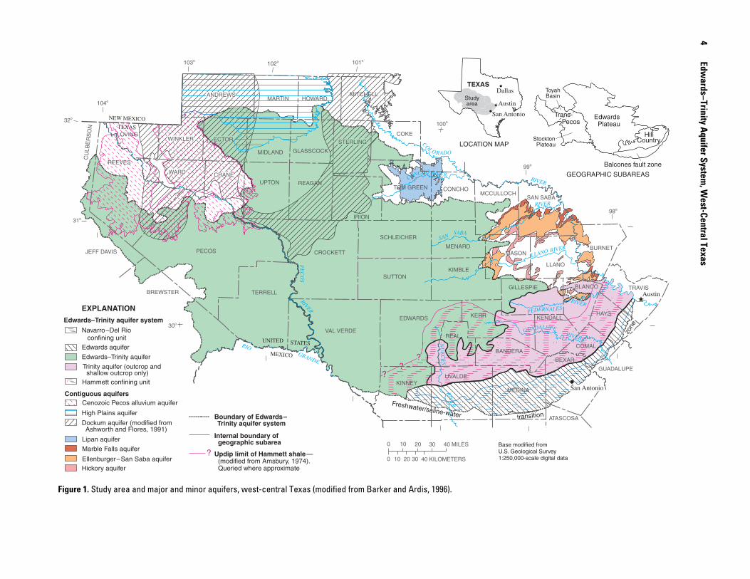
This report is one of a series of reports of the Edwards–Trinity RASA. This report describes the hydrogeology, ground-water use, and ground-water flow in the major aquifers of the Edwards–Trinity aquifer system and contiguous, hydraulically connected units within the study area. The study area is divided into four geographic subareas: Trans-Pecos, Edwards Plateau, Hill Country, and Balcones fault zone (fig. 1). The major aqui-fers within the study area are the Edwards–Trinity in the Trans-Pecos and Edwards Plateau, the Trinity in the Hill Country, and the Edwards in the Balcones fault zone. Important hydraulically connected aquifers are the High Plains aquifer north of the Edwards Plateau, and the Cenozoic Pecos alluvium aquifer adjacent to both the Trans-Pecos and the Edwards Plateau along the Pecos River. Minor contiguous aquifers include the Doc-kum, Ellenburger–San Saba, Marble Falls, and Hickory, and Lipan, which is the alluvial aquifer adjacent to the Colorado River in Tom Green and Concho Counties. These major and minor hydraulically connected aquifers are adjacent to the Edwards–Trinity aquifer system between ground-water divides, such as the Colorado and Pecos Rivers (12,600 mi2). Aquifer names used in this report are those sanctioned by the Texas Water Plan (Texas Water Development Board, 1990).
4 Edw
ards–Trinity Aquifer System
, West-Central Texas
Figure 1. Study area and major and minor aquifers, west-central Texas (modified from Barker and Ardis, 1996).
??
?
?
98o
99o
100o
101o102o103o
104o
32o
31o
30o
0 10 20 30 40 MILES
0 10 20 30 40 KILOMETERS
LOVING
REEVES
CU
LBE
RS
ON
IRION
REAGANUPTON
GLASSCOCKMIDLAND
PECOSJEFF DAVIS
BREWSTER TERRELL
CROCKETT
NEW MEXICOTEXAS
UNITED
MEXICO
STATES
GRANDE
RIO
PE
CO
SRIVER
COL ORADO
RIVER
MITCHELL
COKE
MASON
CONCHOMCCULLOCH
SAN SABA
LLANO
BURNET
GILLESPIE BLANCO TRAVIS
KERR
BANDERA
KENDALLHAYS
BEXAR
GUADALUPE
COMAL
ATASCOSA
MEDINA
EDWARDS
REAL
UVALDEKINNEY
VAL VERDE
SCHLEICHER
MENARD
KIMBLESUTTON
Navarro–Del Rio confining unitEdwards aquifer
Edwards–Trinity aquifer
Trinity aquifer (outcrop and shallow outcrop only)
Edwards–Trinity aquifer system
EXPLANATION
Hammett confining unit
Contiguous aquifersCenozoic Pecos alluvium aquifer
Dockum aquifer (modified from Ashworth and Flores, 1991)
Marble Falls aquifer
Ellenburger–San Saba aquiferHickory aquifer
High Plains aquifer
Updip limit of Hammett shale— (modified from Amsbury, 1974). Queried where approximate
Internal boundary of geographic subarea
Boundary of Edwards– Trinity aquifer system
Edwards Plateau
Trans- Pecos
Hill Country
Balcones fault zone
Freshwater/saline-water transition
zone
Lipan aquifer
GEOGRAPHIC SUBAREAS
ToyahBasin
Stockton Plateau
CONCHO RIVER
SANSABA
RIVER
RIVERLLANO
RIV
ER
RIVERGUADALUPE
NU
EC
ES
PEDERNALESRIVER
Base modified from U.S. Geological Survey1:250,000-scale digital data
TOM GREEN
MARTIN HOWARDANDREWS
WINKLER ECTOR
WARD CRANE
STERLING
TEXAS
Study area
LOCATION MAP
San Antonio
Austin
San Antonio
Austin
Dallas
Introduction 5
The ground-water flow system is conceptually described within this report along with simulation results from the two finite-element models. The regional model was developed to provide a general quantification of the flow system for the majority of the study area and includes the contiguous, hydrau-lically connected units (includes 1,000 mi2 of area beyond the southern boundary of the Balcones fault zone in the low perme-ability downdip part the Cretaceous rocks). The contiguous, hydraulically connected units were included in the simulation in order to extend the model boundaries to ground-water divides that could be defined as no-flow divides or as head-dependent boundaries along rivers where the flow to or from the rivers could be estimated from hydrograph separation techniques (Rutledge, 1998; Kuniansky, 1989). Kuniansky and Holligan (1994) describe the details of the steady-state regional model calibration and sensitivity analysis. The steady-state simula-tions were for predevelopment conditions and for winter 1974–75 conditions. The winter of 1974–75 (December 1974 through February 1975) was selected for simulation for three reasons: (1) the system is closest to steady state during winter; (2) less ground water is lost to evaporation, irrigation withdrawals, and transpiration during winter; and (3) water use in parts of the study area had peaked during this period.
A one-layer model was adequate to simulate flow for the majority of the study area but inadequate for the Hill Country and the Balcones fault zone. In general, a ground-water flow system can be approximated with one layer if the thickness of the aquifer is much less than the horizontal dimension of the system. In the case of the regional system, the horizontal dimension is more than four orders of magnitude greater than the average thickness of the system. One regionally mappable confining unit is a gulfward thickening unit of mudstone and clay (Amsbury, 1974), the Hammett shale, within the Hill Country and Balcones fault zone. This unit forms a vertical division within the Trinity aquifer in the Hill Country, and this aquifer is split into multiple aquifers for local studies (Ashworth, 1983). At the southern segment of the Balcones fault zone, the Navarro–Del Rio confining unit overlies the Edwards aquifer. Thus, a multilayer model was developed for the subregion that includes the Hill Country and Balcones fault zone, and part of the Edwards Plateau.
The subregional model area extends into the southeastern part of the Edwards Plateau north and west of the Hill Country and Balcones fault zone where the aquifers form a shallow, mostly unconfined ground-water flow system. During 1993, the scope of the subregional model was modified to better simulate the hydrology of endangered and threatened species habitats near major springs. The subregional model mesh was designed to be site specific at Comal, San Marcos, and Barton Springs extending to hydrologic divides just beyond the two geographic subareas. The subregional model was designed to be multilayer in order to estimate vertical leakage between the Trinity aquifer and the Edwards aquifer. The subregional model development, boundary conditions, sources and sinks are documented in this report. Initial conditions, time-step size, calibration, and sensi-
tivity analysis of the subregional multilayer model are docu-mented in appendix A of this report.
Although the computer programs developed for simulation and pre- and postprocessing of the data are major elements of the work undertaken, it is not within the scope of this report to document and describe the computer programs. Some of these programs are documented in Kuniansky, 1990a; Lowther and Kuniansky, 1992; Torak, 1992a,b; and Cooley, 1992.
Calibration of the subregional model was accomplished using monthly stress periods from 1978–89. The calibration period, 1978–89, represents more recent postdevelopment pumping stresses with slightly above average long-term recharge (1934–90) with a few extremely wet periods. Texas Water Development Board (Thorkildsen and McElhaney, written commun., 1993) complied the monthly ground-water withdrawals for the San Antonio area. Water use for the Austin area and the Hill Country were compiled from data obtained from the Texas Water Development Board. Well locations for the Hill Country and Balcones fault zone were obtained from the Texas Natural Resources and Conservation Commission (Ed Bloch, 1993 written commun.), formerly the Texas Water Commission.
Previous Studies
Numerous reports have been written about the geology and ground-water resources of west-central Texas. Barker and Ardis (1996) provide a comprehensive listing of reports on geology alone. Numerous reports of well data and county ground-water investigative reports are cited in the Selected References section of this report. Reports of significance to the study area that are statewide in scope include: Brune’s (1975 and 1981) reports on springs; Carr’s (1967) report on climate; Gillett and Janca’s (1965) report on irrigation; Hill and Vaughan’s (1898) report on ground water; Muller and Price’s (1979) report on ground-water availability; Kane’s (1967) report on reservoir evaporation rates; Knape’s (1984) report on underground injection operations; Larkin and Bomar’s (1983) climatic atlas; Laxson’s (1960) report on resistivities and chemical analysis of formations; Mount and others (1967) report on ground-water availability along the Colorado River Basin; Myers’ (1969) compilation of aquifer tests; Rechenthin and Smith’s (1966) report on grassland restoration effects on water yields; Texas Department of Agriculture and U.S. Department of Agriculture’s (1985) compilation of county statistics; Texas Water Commission’s (1988) water-quality inventory; Texas Water Development Board’s (1986, 1991) irrigation surveys; Winslow and Kister’s (1956) report on saline-water resources; and Zabecza and Szabo’s (1986) report on natural radioactivity in ground water. Reports of significance to the geology of the Edwards–Trinity aquifer system are Fisher and Rodda, 1969; Flawn and others, 1961; Lozo, 1959; Lozo and Smith, 1964; Rose, 1972; Smith, 1974; and Tucker, 1962.
Reports relating to streamflow losses to the Edwards aqui-fer include Kuniansky, 1989; Land and others, 1983; Reeves
6 Edwards–Trinity Aquifer System, West-Central Texas
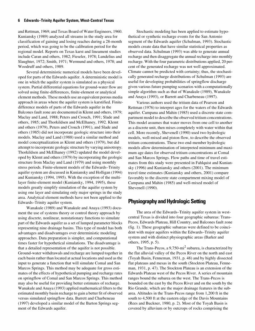
and Rettman, 1969; and Texas Board of Water Engineers, 1960. Kuniansky (1989) analyzed all streams in the study area for classification of gaining and losing reaches during a 28-month period, which was going to be the calibration period for the regional model. Reports on Texas karst and lineament studies include Caran and others, 1982; Fieseler, 1978; Lundelius and Slaughter, 1972; Smith, 1971; Wermund and others, 1978; and Woodruff and others, 1989.
Several deterministic numerical models have been devel-oped for parts of the Edwards aquifer. A deterministic model is one in which the aquifer system is simulated as a physical system. Partial differential equations for ground-water flow are solved using finite-differences, finite-element or analytical element methods. These models use an equivalent porous media approach in areas where the aquifer system is karstified. Finite-difference models of parts of the Edwards aquifer in the Balcones fault zone are documented in Klemt and others, 1979; Maclay and Land, 1988; Peters and Crouch, 1991; Slade and others, 1985; and Thorkildsen and McElhaney, 1992. Klemt and others (1979), Peters and Crouch (1991), and Slade and others (1985) did not incorporate geologic structure into their models. Maclay and Land (1988) used a similar method and model conceptualization as Klemt and others (1979), but did attempt to incorporate geologic structure by varying anisotropy. Thorkildsen and McElhaney (1992) updated the model devel-oped by Klemt and others (1979) by incorporating the geologic structure from Maclay and Land (1979) and using monthly stress periods. Finite-element models of the Edwards–Trinity aquifer system are discussed in Kuniansky and Holligan (1994) and Kuniansky (1994, 1995). With the exception of the multi-layer finite-element model (Kuniansky, 1994, 1995), these models greatly simplify simulation of the aquifer system by using one layer and simulating only major springs in the study area. Analytical element methods have not been applied to the Edwards–Trinity aquifer system.
Wanakule (1989) and Wanakule and Anaya (1993) docu-ment the use of systems theory or control theory approach by using discrete, nonlinear, nonstationary functions to simulate part of the Edwards aquifer as a set of lumped parameter blocks representing nine drainage basins. This type of model has both advantages and disadvantages over deterministic modeling approaches. Data preparation is simpler, and computational times faster for hypothetical simulations. The disadvantage is that a detailed representation of the aquifer is not possible. Ground-water withdrawals and recharge are lumped together in each basin rather than located at actual locations and used as the input to generate a function that will simulate Comal and San Marcos Springs. This method may be adequate for gross esti-mates of the effects of hypothetical pumping and recharge rates on springflow of Comal and San Marcos Springs. This method may also be useful for providing better estimates of recharge. Wanakule and Anaya (1993) applied mathematical filters to the estimated monthly basin recharge to gain a better fit of observed versus simulated springflow data. Barrett and Charbeneau (1997) developed a similar model of the Barton Springs seg-ment of the Edwards aquifer.
Stochastic modeling has been applied to estimate hypo-thetical or synthetic recharge events for the San Antonio segment of the Edwards aquifer (Schulman, 1993). Stochastic models create data that have similar statistical properties as observed data. Schulman (1993) was able to generate annual recharge and then disaggregate the annual recharge into monthly recharge. With the four parametric distributions applied, 20 per-cent of the generated recharge was not well approximated. Climate cannot be predicted with certainty; thus, the stochasti-cally generated recharge distributions of Schulman (1993) are useful for developing probabilities of springflow discharge given various future pumping scenarios with a computationally simple algorithm such as that of Wanakule (1989), Wanakule and Anaya (1993), or Barrett and Charbeneau (1997).
Various authors used the tritium data of Pearson and Rettman (1976) to interpret ages for the waters of the Edwards aquifer. Campana and Mahin (1985) used a discrete state com-partment model to describe the observed tritium concentrations. This model assumes that water moves from one cell to another as a discrete unit, then mixes completely with water within that cell. More recently, Shevenell (1990) used two hydrologic models, well-mixed and piston flow, to describe the observed tritium concentrations. These two end-member hydrologic models allow determination of interpreted minimum and maxi-mum age dates for observed tritium concentrations at Comal and San Marcos Springs. Flow paths and time of travel esti-mates from this study were presented in Fahlquist and Kunian-sky (1996) and Kuniansky and others (2001). The minimum travel time estimates (Kuniansky and others, 2001) compare favorably to the discrete state compartment mixing model of Campana and Mahin (1985) and well-mixed model of Shevenell (1990).
Physiography and Hydrologic Setting
The area of the Edwards–Trinity aquifer system in west-central Texas is divided into four geographic subareas: Trans-Pecos, Edwards Plateau, Hill Country, and Balcones fault zone (fig. 1). These geographic subareas were defined to be coinci-dent with major aquifers within the Edwards–Trinity aquifer system and with distinct physiographic areas (Barker and others, 1995, p. 5).
The Trans-Pecos, a 9,750-mi2 subarea, is characterized by the flat alluvial valley of the Pecos River on the north and east (Toyah Basin, Fenneman, 1931, p. 48) and by highly dissected flat plateaus and mesas in the south (Stockton Plateau, Fenne-man, 1931, p. 47). The Stockton Plateau is an extension of the Edwards Plateau west of the Pecos River. A series of mountain ranges bound the subarea on the west. The Trans-Pecos is bounded on the east by the Pecos River and on the south by the Rio Grande, which are the major drainage features in the sub-area. Altitudes in the Trans-Pecos range from 1,200 ft in the south to 4,500 ft at the eastern edge of the Davis Mountains (Rees and Buckner, 1980, p. 2). Most of the Toyah Basin is covered by alluvium or by outcrops of rocks comprising the
Introduction 7
Edwards–Trinity aquifer. The southern part of the Trans-Pecos, the Stockton Plateau, has more rugged terrain of exposed car-bonate rocks lacking any alluvial mantle.
The Edwards Plateau, a 23,750-mi2 subarea, in the center of the study area is characterized by “…rolling plains to flat tableland and rugged, steep-walled canyons and draws…” rang-ing in altitude from 3,300 to 1,000 ft (Walker, 1979, p. 7). This relatively flat surface slopes gradually from Ector County on the northwest to Edwards County on the southeast at a rate of approximately 5 ft/mi. The topography slopes steeply near the Pecos River and the Rio Grande on the western and southwest-ern boundaries of the subarea, respectively, resulting in more rugged terrain. The northeastern boundary is incised by the headwaters of the Concho, San Saba, and Llano Rivers, which drain into the Colorado River. The surface of the Edwards Pla-teau is a partially saturated mantle of rocks of the Edwards Group (Rose, 1972) in the east and stratigraphic equivalents of the Edwards Group in the west (Smith and Brown, 1983). These surficial Cretaceous rocks have moderate permeability, but large infiltration capacity (Maclay and Land, 1988, p. 4). Caves are present mostly within the southern Edwards Plateau, but little surface expression of karst is evident.
The Hill Country, a 5,500-mi2 subarea, is characterized by rough rolling terrain dissected by the headwaters of the streams within the Nueces and Guadalupe River Basins. These streams have eroded headward into the Edwards Plateau forming nar-row valleys with steep walls of mostly carbonate rock. Wider stream valleys along the major streams may result from lateral cutting and karstification during the past when rainfall was more plentiful (Wermund and others, 1974, p. 425). Land-sur-face altitudes in the Hill Country range from 800 to 2,400 ft (Ashworth, 1983, p. 2). In the western part of the Hill Country, rocks of the Edwards Group (Rose, 1972), predominantly com-posed of limestone and dolomite, cap the hills. The surficial rocks in the eastern part of the Hill Country are largely those of the Glen Rose Limestone and consist of marl, shale, and carbon-ate rocks of relatively low permeability.
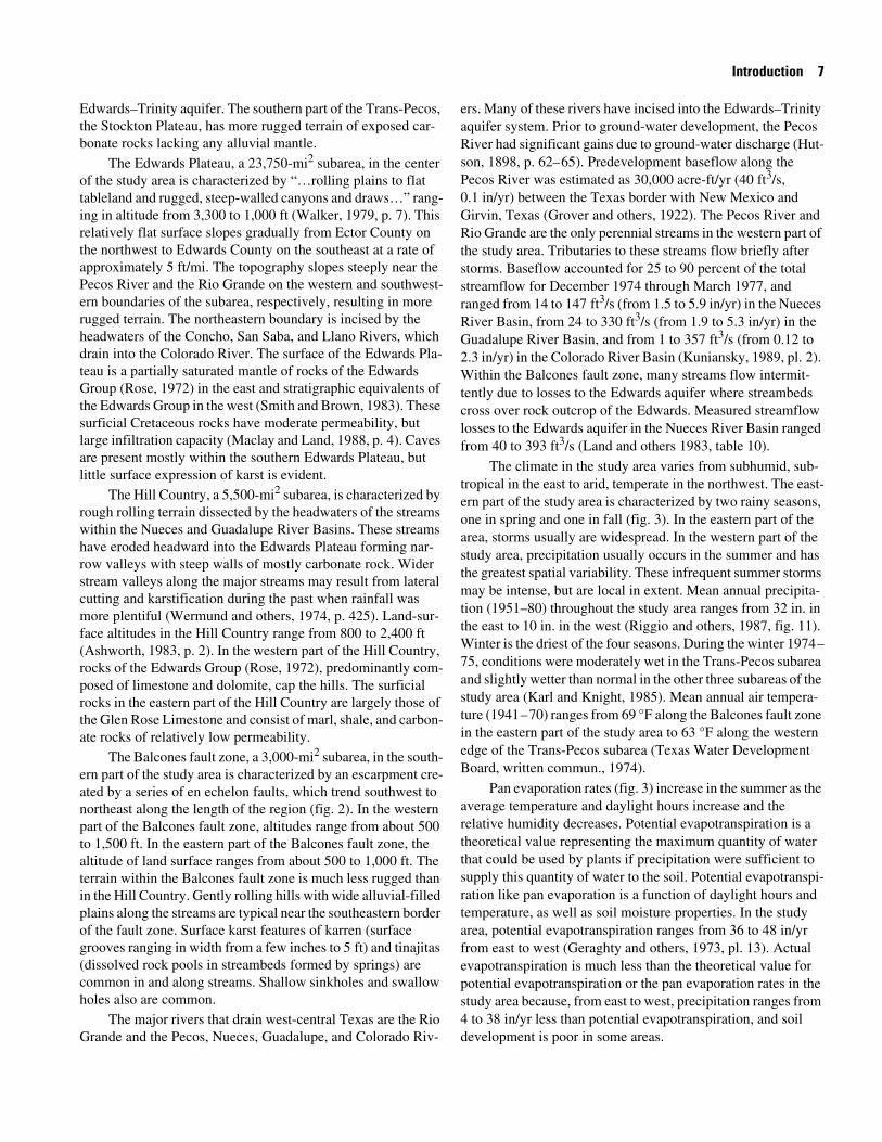
The Balcones fault zone, a 3,000-mi2 subarea, in the south-ern part of the study area is characterized by an escarpment cre-ated by a series of en echelon faults, which trend southwest to northeast along the length of the region (fig. 2). In the western part of the Balcones fault zone, altitudes range from about 500 to 1,500 ft. In the eastern part of the Balcones fault zone, the altitude of land surface ranges from about 500 to 1,000 ft. The terrain within the Balcones fault zone is much less rugged than in the Hill Country. Gently rolling hills with wide alluvial-filled plains along the streams are typical near the southeastern border of the fault zone. Surface karst features of karren (surface grooves ranging in width from a few inches to 5 ft) and tinajitas (dissolved rock pools in streambeds formed by springs) are common in and along streams. Shallow sinkholes and swallow holes also are common.
The major rivers that drain west-central Texas are the Rio Grande and the Pecos, Nueces, Guadalupe, and Colorado Riv-
ers. Many of these rivers have incised into the Edwards–Trinity aquifer system. Prior to ground-water development, the Pecos River had significant gains due to ground-water discharge (Hut-son, 1898, p. 62–65). Predevelopment baseflow along the Pecos River was estimated as 30,000 acre-ft/yr (40 ft3/s,0.1 in/yr) between the Texas border with New Mexico and Girvin, Texas (Grover and others, 1922). The Pecos River and Rio Grande are the only perennial streams in the western part of the study area. Tributaries to these streams flow briefly after storms. Baseflow accounted for 25 to 90 percent of the total streamflow for December 1974 through March 1977, and ranged from 14 to 147 ft3/s (from 1.5 to 5.9 in/yr) in the Nueces River Basin, from 24 to 330 ft3/s (from 1.9 to 5.3 in/yr) in the Guadalupe River Basin, and from 1 to 357 ft3/s (from 0.12 to 2.3 in/yr) in the Colorado River Basin (Kuniansky, 1989, pl. 2). Within the Balcones fault zone, many streams flow intermit-tently due to losses to the Edwards aquifer where streambeds cross over rock outcrop of the Edwards. Measured streamflow losses to the Edwards aquifer in the Nueces River Basin ranged from 40 to 393 ft3/s (Land and others 1983, table 10).
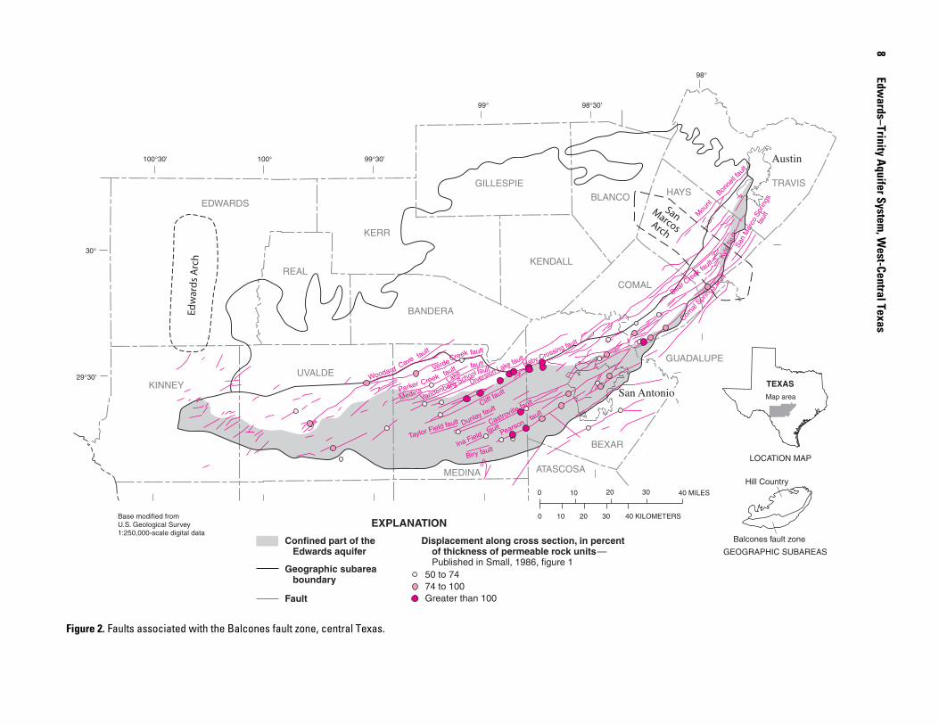
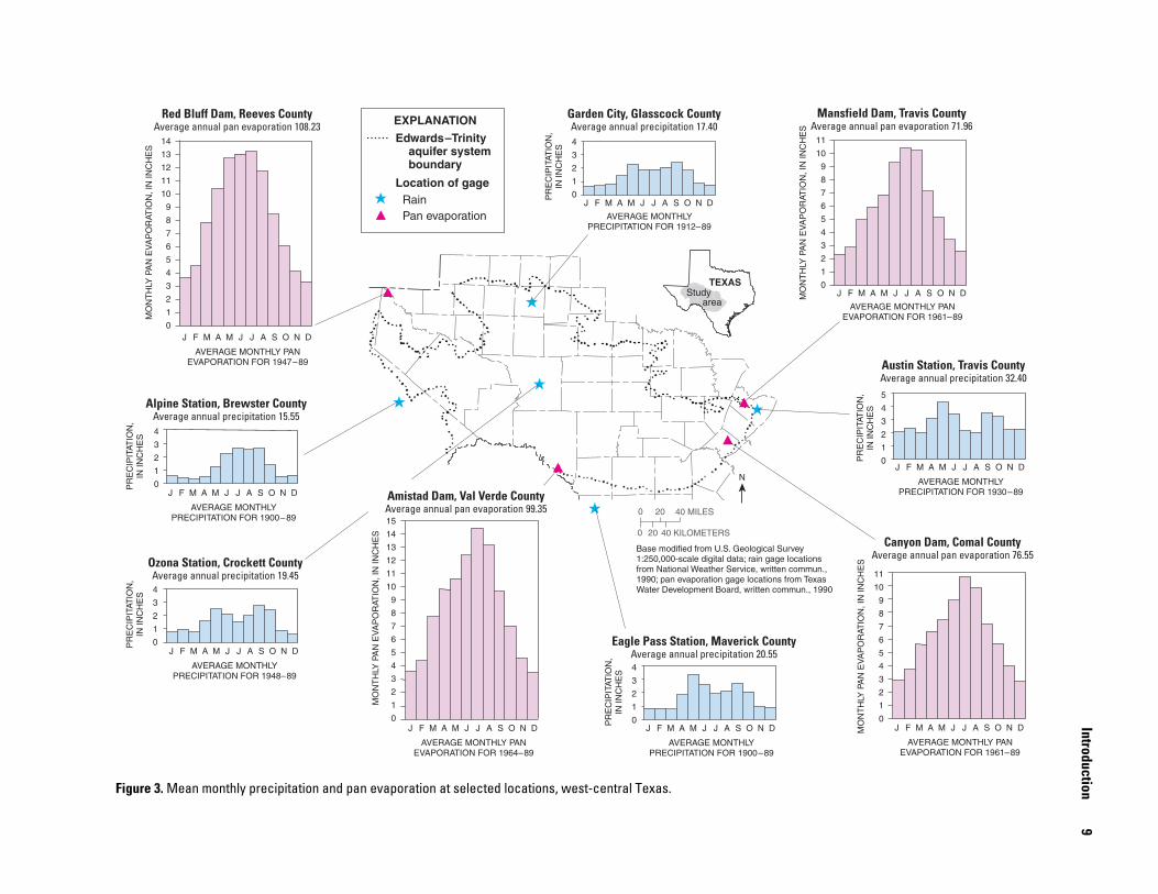
The climate in the study area varies from subhumid, sub-tropical in the east to arid, temperate in the northwest. The east-ern part of the study area is characterized by two rainy seasons, one in spring and one in fall (fig. 3). In the eastern part of the area, storms usually are widespread. In the western part of the study area, precipitation usually occurs in the summer and has the greatest spatial variability. These infrequent summer storms may be intense, but are local in extent. Mean annual precipita-tion (1951–80) throughout the study area ranges from 32 in. in the east to 10 in. in the west (Riggio and others, 1987, fig. 11). Winter is the driest of the four seasons. During the winter 1974–75, conditions were moderately wet in the Trans-Pecos subarea and slightly wetter than normal in the other three subareas of the study area (Karl and Knight, 1985). Mean annual air tempera-ture (1941–70) ranges from 69 °F along the Balcones fault zone in the eastern part of the study area to 63 °F along the western edge of the Trans-Pecos subarea (Texas Water Development Board, written commun., 1974).
Pan evaporation rates (fig. 3) increase in the summer as the average temperature and daylight hours increase and the relative humidity decreases. Potential evapotranspiration is a theoretical value representing the maximum quantity of water that could be used by plants if precipitation were sufficient to supply this quantity of water to the soil. Potential evapotranspi-ration like pan evaporation is a function of daylight hours and temperature, as well as soil moisture properties. In the study area, potential evapotranspiration ranges from 36 to 48 in/yr from east to west (Geraghty and others, 1973, pl. 13). Actual evapotranspiration is much less than the theoretical value for potential evapotranspiration or the pan evaporation rates in the study area because, from east to west, precipitation ranges from 4 to 38 in/yr less than potential evapotranspiration, and soil development is poor in some areas.
8 Edw
ards–Trinity Aquifer System
, West-Central Texas
Figure 2. Faults associated with the Balcones fault zone, central Texas.
98°
99° 98°30'
99°30'100°30'
29°30'
100°
30°
Austin
San Antonio
Mou
nt
Bon
nell f
ault
San
Mar
co S
prin
gs
fa
ult
Kyle
faul
t
Comal
Spring
s fau
lt
Bear Creek f
ault
Haby Crossing fault
Diversion Lake fault
Cliff fault
Dunlay fault
Ina Field fault
Biry fault
PearsonCastroville fault
Taylor Field fault
Vandenberg
Verde
Lake
MedinaParkerWoodard
Creek
Cavefault
faultfault
fault
faultfault
School
Creek
GILLESPIE
BLANCO
KENDALL
TRAVIS
KERR
BANDERA
HAYS
BEXAR
GUADALUPE
COMAL
ATASCOSAMEDINA
EDWARDS
REAL
UVALDEKINNEY
0 10 20 30
Base modified from U.S. Geological Survey1:250,000-scale digital data
40 MILES
40 KILOMETERS0 10 20 30
Confined part of the Edwards aquifer
Displacement along cross section, in percent of thickness of permeable rock units— Published in Small, 1986, figure 1
Fault
Geographic subarea boundary
EXPLANATION
50 to 7474 to 100Greater than 100
TEXAS
Map area
Hill Country
Balcones fault zone
GEOGRAPHIC SUBAREAS
LOCATION MAP
Introduction9
Figure 3. Mean monthly precipitation and pan evaporation at selected locations, west-central Texas.
14
13
12
11
10
9
8
7
6
5
4
3
2
1
0
MO
NT
HLY
PA
N E
VA
PO
RAT
ION
, IN
INC
HE
S
J F M A M J J A S O N D
AVERAGE MONTHLY PANEVAPORATION FOR 1947–89
Red Bluff Dam, Reeves CountyAverage annual pan evaporation 108.23
Mansfield Dam, Travis CountyAverage annual pan evaporation 71.96
Ozona Station, Crockett CountyAverage annual precipitation 19.45
Alpine Station, Brewster CountyAverage annual precipitation 15.55
Canyon Dam, Comal CountyAverage annual pan evaporation 76.55
4
3
2
1
0
15
14
13
12
11
10
9
8
7
6
5
4
3
2
1
0
11
10
9
8
7
6
5
4
3
2
1
0
11
10
9
8
7
6
5
4
3
2
1
0
PR
EC
IPIT
ATIO
N,
IN IN
CH
ES
4
3
2
1
0PR
EC
IPIT
ATIO
N,
IN IN
CH
ES
MO
NT
HLY
PA
N E
VA
PO
RAT
ION
, IN
INC
HE
S
MO
NT
HLY
PA
N E
VA
PO
RAT
ION
, IN
INC
HE
S
MO
NT
HLY
PA
N E
VA
PO
RAT
ION
, IN
INC
HE
S
J F M A M J J A S O N D
AVERAGE MONTHLYPRECIPITATION FOR 1948–89
J F M A M J J A S O N D
AVERAGE MONTHLYPRECIPITATION FOR 1900–89
Eagle Pass Station, Maverick CountyAverage annual precipitation 20.55
Austin Station, Travis CountyAverage annual precipitation 32.40
4
3
2
1
0PR
EC
IPIT
ATIO
N,
IN IN
CH
ES
5
4
3
2
1
0PR
EC
IPIT
ATIO
N,
IN IN
CH
ES
Garden City, Glasscock CountyAverage annual precipitation 17.404
3
2
1
0PR
EC
IPIT
ATIO
N,
IN IN
CH
ES
J F M A M J J A S O N D
AVERAGE MONTHLYPRECIPITATION FOR 1900–89
J F M A M J J A S O N D
AVERAGE MONTHLYPRECIPITATION FOR 1930–89
J F M A M J J A S O N D
AVERAGE MONTHLYPRECIPITATION FOR 1912–89
J F M A M J J A S O N D
AVERAGE MONTHLY PANEVAPORATION FOR 1964–89
J F M A M J J A S O N D
AVERAGE MONTHLY PANEVAPORATION FOR 1961–89
J F M A M J J A S O N D
AVERAGE MONTHLY PANEVAPORATION FOR 1961–89
Location of gage
Edwards–Trinity aquifer system boundary
EXPLANATION
RainPan evaporation
Amistad Dam, Val Verde CountyAverage annual pan evaporation 99.35
TEXASStudy area
Base modified from U.S. Geological Survey1:250,000-scale digital data; rain gage locations from National Weather Service, written commun., 1990; pan evaporation gage locations from Texas Water Development Board, written commun., 1990
0 20 40 MILES
0 20 40 KILOMETERS
N
10 Edwards–Trinity Aquifer System, West-Central Texas
Soil development is poor across most of the arid and semi-arid regions of the Trans-Pecos, Edwards Plateau, and Hill Country. Consequently, soil thickness is commonly less than 1 ft in the Trans-Pecos where soils are clay loams overlying rough, stony terrain vegetated by desert shrubs. In the Edwards Plateau, soils tend to be calcareous stony clays vegetated by desert shrubs in the west and by juniper, oak, and mesquite in the east. The Hill Country has soils and vegetation similar to those of the Edwards Plateau. In the northeastern part of the Balcones fault zone, soils are calcareous clays, clayey loams, and sandy loams with some prairie vegetation. In the southwest-ern part of the Balcones fault zone, west of San Antonio, the vegetation changes to juniper, oak, and mesquite, which tolerate arid conditions (Kier and others, 1977).
HYDROGEOLOGY
Edwards–Trinity Aquifer System and Contiguous Hydraulically Connected Units
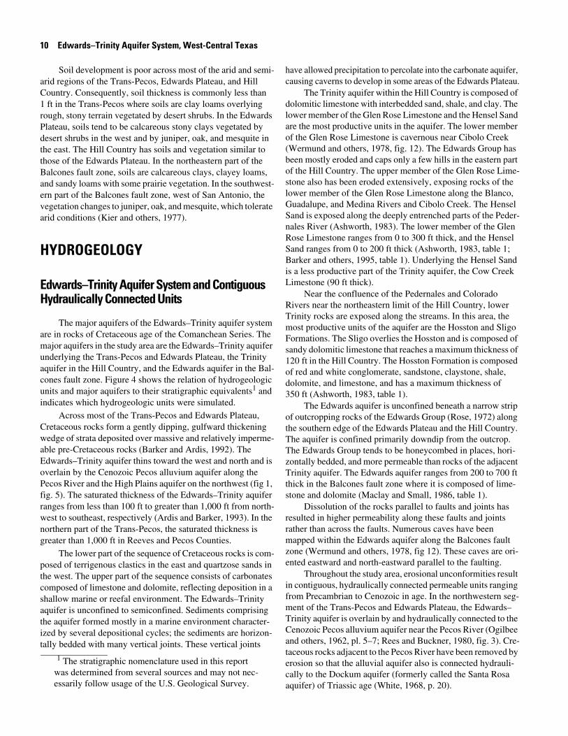
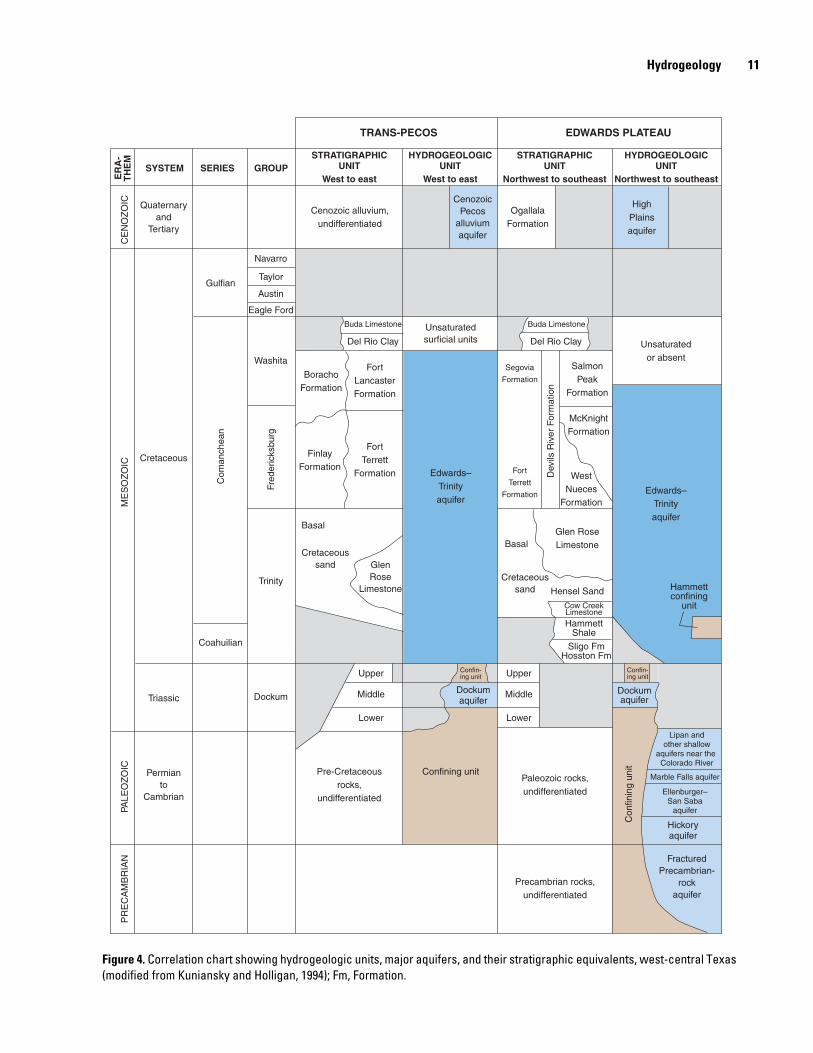
The major aquifers of the Edwards–Trinity aquifer system are in rocks of Cretaceous age of the Comanchean Series. The major aquifers in the study area are the Edwards–Trinity aquifer underlying the Trans-Pecos and Edwards Plateau, the Trinity aquifer in the Hill Country, and the Edwards aquifer in the Bal-cones fault zone. Figure 4 shows the relation of hydrogeologic units and major aquifers to their stratigraphic equivalents1 and indicates which hydrogeologic units were simulated.
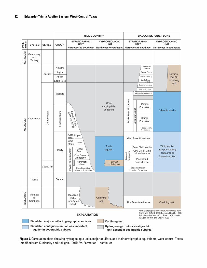
Across most of the Trans-Pecos and Edwards Plateau, Cretaceous rocks form a gently dipping, gulfward thickening wedge of strata deposited over massive and relatively imperme-able pre-Cretaceous rocks (Barker and Ardis, 1992). The Edwards–Trinity aquifer thins toward the west and north and is overlain by the Cenozoic Pecos alluvium aquifer along the Pecos River and the High Plains aquifer on the northwest (fig 1, fig. 5). The saturated thickness of the Edwards–Trinity aquifer ranges from less than 100 ft to greater than 1,000 ft from north-west to southeast, respectively (Ardis and Barker, 1993). In the northern part of the Trans-Pecos, the saturated thickness is greater than 1,000 ft in Reeves and Pecos Counties.
The lower part of the sequence of Cretaceous rocks is com-posed of terrigenous clastics in the east and quartzose sands in the west. The upper part of the sequence consists of carbonates composed of limestone and dolomite, reflecting deposition in a shallow marine or reefal environment. The Edwards–Trinity aquifer is unconfined to semiconfined. Sediments comprising the aquifer formed mostly in a marine environment character-ized by several depositional cycles; the sediments are horizon-tally bedded with many vertical joints. These vertical joints
have allowed precipitation to percolate into the carbonate aquifer, causing caverns to develop in some areas of the Edwards Plateau.
The Trinity aquifer within the Hill Country is composed of dolomitic limestone with interbedded sand, shale, and clay. The lower member of the Glen Rose Limestone and the Hensel Sand are the most productive units in the aquifer. The lower member of the Glen Rose Limestone is cavernous near Cibolo Creek (Wermund and others, 1978, fig. 12). The Edwards Group has been mostly eroded and caps only a few hills in the eastern part of the Hill Country. The upper member of the Glen Rose Lime-stone also has been eroded extensively, exposing rocks of the lower member of the Glen Rose Limestone along the Blanco, Guadalupe, and Medina Rivers and Cibolo Creek. The Hensel Sand is exposed along the deeply entrenched parts of the Peder-nales River (Ashworth, 1983). The lower member of the Glen Rose Limestone ranges from 0 to 300 ft thick, and the Hensel Sand ranges from 0 to 200 ft thick (Ashworth, 1983, table 1; Barker and others, 1995, table 1). Underlying the Hensel Sand is a less productive part of the Trinity aquifer, the Cow Creek Limestone (90 ft thick).
Near the confluence of the Pedernales and Colorado Rivers near the northeastern limit of the Hill Country, lower Trinity rocks are exposed along the streams. In this area, the most productive units of the aquifer are the Hosston and Sligo Formations. The Sligo overlies the Hosston and is composed of sandy dolomitic limestone that reaches a maximum thickness of 120 ft in the Hill Country. The Hosston Formation is composed of red and white conglomerate, sandstone, claystone, shale, dolomite, and limestone, and has a maximum thickness of 350 ft (Ashworth, 1983, table 1).
The Edwards aquifer is unconfined beneath a narrow strip of outcropping rocks of the Edwards Group (Rose, 1972) along the southern edge of the Edwards Plateau and the Hill Country. The aquifer is confined primarily downdip from the outcrop. The Edwards Group tends to be honeycombed in places, hori-zontally bedded, and more permeable than rocks of the adjacent Trinity aquifer. The Edwards aquifer ranges from 200 to 700 ft thick in the Balcones fault zone where it is composed of lime-stone and dolomite (Maclay and Small, 1986, table 1).
Dissolution of the rocks parallel to faults and joints has resulted in higher permeability along these faults and joints rather than across the faults. Numerous caves have been mapped within the Edwards aquifer along the Balcones fault zone (Wermund and others, 1978, fig 12). These caves are ori-ented eastward and north-eastward parallel to the faulting.
Throughout the study area, erosional unconformities result in contiguous, hydraulically connected permeable units ranging from Precambrian to Cenozoic in age. In the northwestern seg-ment of the Trans-Pecos and Edwards Plateau, the Edwards–Trinity aquifer is overlain by and hydraulically connected to the Cenozoic Pecos alluvium aquifer near the Pecos River (Ogilbee and others, 1962, pl. 5–7; Rees and Buckner, 1980, fig. 3). Cre-taceous rocks adjacent to the Pecos River have been removed by erosion so that the alluvial aquifer also is connected hydrauli-cally to the Dockum aquifer (formerly called the Santa Rosa aquifer) of Triassic age (White, 1968, p. 20).
1 The stratigraphic nomenclature used in this report was determined from several sources and may not nec-essarily follow usage of the U.S. Geological Survey.
Hydrogeology 11
Figure 4. Correlation chart showing hydrogeologic units, major aquifers, and their stratigraphic equivalents, west-central Texas (modified from Kuniansky and Holligan, 1994); Fm, Formation.
Quaternaryand
Tertiary
Cenozoic alluvium,undifferentiated
CenozoicPecos
alluviumaquifer
OgallalaFormation
Buda LimestoneBuda Limestone
Del Rio ClayDel Rio Clay
SalmonPeak
Formation
McKnightFormation
WestNueces
Formation
Glen RoseLimestone
GlenRose
Limestone Hensel Sand
Paleozoic rocks,undifferentiated
Pre-Cretaceousrocks,
undifferentiated
Confining unit
Confin-ing unit
Confin-ing unit
Precambrian rocks,undifferentiated
HammettShale
Cow CreekLimestone
Sligo FmHosston Fm
Dev
ils R
iver
For
mat
ion
Fort
Terrett
Formation
FortTerrett
Formation
FortLancasterFormation
Edwards–Trinityaquifer
Unsaturatedsurficial units
Basal
Basal
Upper
MiddleDockumaquifer
Lower
Upper
Middle
Lower
Cretaceoussand
Cretaceoussand
Segovia
FormationBorachoFormation
FinlayFormation
Cretaceous
Triassic
Permianto
Cambrian
PALE
OZ
OIC
ME
SO
ZO
ICC
EN
OZ
OIC
SYSTEM SERIES GROUPSTRATIGRAPHIC
UNITWest to east West to east Northwest to southeast Northwest to southeast
TRANS-PECOS EDWARDS PLATEAU
STRATIGRAPHICUNIT
HYDROGEOLOGICUNIT
HYDROGEOLOGICUNIT
ER
A-
TH
EM
PR
EC
AM
BR
IAN
Gulfian
Navarro
Eagle Ford
Washita
Trinity
Dockum
Coahuilian
Fred
eric
ksbu
rg
Com
anch
ean
Austin
Taylor
HighPlainsaquifer
Edwards–Trinityaquifer
Dockumaquifer
Marble Falls aquifer
Ellenburger–San Saba
aquifer
Lipan andother shallow
aquifers near the Colorado River
Hickoryaquifer
FracturedPrecambrian-
rockaquifer
Con
finin
g un
it
Hammettconfining
unit
Unsaturatedor absent
12 Edwards–Trinity Aquifer System, West-Central Texas
Figure 4. Correlation chart showing hydrogeologic units, major aquifers, and their stratigraphic equivalents, west-central Texas (modified from Kuniansky and Holligan, 1994); Fm, Formation—continued.
HILL COUNTRY BALCONES FAULT ZONE
Northwest to southeast Northwest to southeast
STRATIGRAPHICUNIT
HYDROGEOLOGICUNIT
Northwest to southeast Northwest to southeast
STRATIGRAPHICUNIT
HYDROGEOLOGICUNIT
Glen Rose Limestone
Bexar Shale Member
Hammettconfining unit
Hammettshale
Cow Creek Lime-stone Member
Cow CreekLimestone
HenselSand
Pine IslandSand Member
Trinityaquifer
GlenRoseLime-stone
Unitscapping hills
or absent
Upper
Lower
Trinity aquifer(low permeability
compared toEdwards aquifer)
Edwards aquiferEdw
ards Group
(of Rose, 1972)
PersonFormation
Del Rio Clay
Buda Limestone
Eagle Ford Group
Austin Group
Taylor Group
NavarroGroup
Navarro–Del Rio
confiningunit
KainerFormation
Basal nodularmember
Georgetown Formation
Confiningunit Confining unitUndifferentiated rocks
Paleozoicrocks,
undifferen-tiated
Sligo FormationHosston Formation
Pea
rsal
lF
orm
atio
nD
evils
Riv
er F
orm
atio
n
Edw
ards
Gro
up
Trav
is P
eak
equi
vale
nt
Sligo FormationHosston Formation
Quaternaryand
Tertiary
Cretaceous
Triassic
Permianto
Cambrian
PALE
OZ
OIC
ME
SO
ZO
ICC
EN
OZ
OIC
SYSTEM SERIES GROUP
ER
A-
TH
EM
Gulfian
Navarro
Eagle Ford
Washita
Trinity
Dockum
Coahuilian
Fred
eric
ksbu
rg
Com
anch
ean
Austin
Taylor
Rock-stratigraphic nomenclature modified from Brand and Deford, 1958; Lozo and Smith, 1964; Stricklin and others, 1971; Rose, 1972; Loucks, 1977; and Smith and Brown, 1983
EXPLANATION
Simulated major aquifer in geographic subarea Confining unit
Hydrogeologic unit or stratigraphic unit absent in geographic subarea
Simulated contiguous unit or less important aquifer in geographic subarea
Hydrogeology
13
Figure 5. Generalized section showing the geologic or hydrogeologic units simulated as one layer in the regional model, west-central Texas (modified from Kuniansky and Holligan, 1994); Fm, Formation.
A CB
Tertiary volcanics
Basal Cretaceous sand
Boracho Fm
Permian andTriassic rocks
Permian and Triassic sand and red beds
Quaternaryalluvium
SegoviaFormation
Fort TerrettFormation
Dockumaquifer Paleozoic rocks
Marble
Fall
s Fm
Ellenb
urge
r Fm
Hickor
y Fm
Hic
kory
Fm
Precambrian
Hensel Sand
HenselSand
Lower GlenRose Limestone
Mat
ch li
ne—
See
follo
win
g pa
ge
FEET
4,000
3,000
2,000
1,000
NGVDOF 1929
1,000
2,000
3,000
4,000
5,000
6,000Modified from Rees and Buckner, 1980, fig.3; White, 1971, fig. 25 Modified from Mount and others, 1967, plate 4; Walker, 1979, fig. 11
BE
ND
IN
SE
CT
ION
BE
ND
IN
SE
CT
ION
Dockum Group
VERTICAL SCALE GREATLY EXAGERRATEDNOT TO SCALE
Edwards Plateau
Trans-Pecos
Hill Country
Balconesfault zone
A BC
D
TEXAS
14 Edw
ards–Trinity Aquifer System
, West-Central Texas
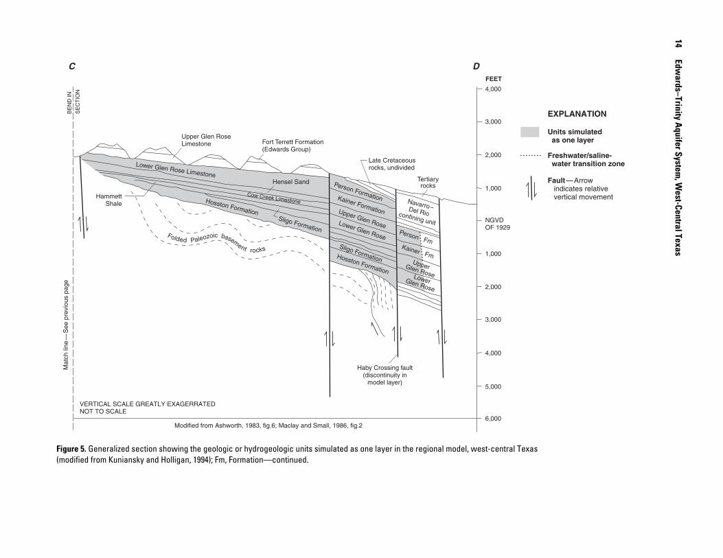
Figure 5. Generalized section showing the geologic or hydrogeologic units simulated as one layer in the regional model, west-central Texas (modified from Kuniansky and Holligan, 1994); Fm, Formation—continued.
C DM
atch
line
—S
ee p
revi
ous
page
FEET
4,000
3,000
2,000
1,000
NGVDOF 1929
1,000
2,000
3,000
4,000
5,000
6,000Modified from Ashworth, 1983, fig.6; Maclay and Small, 1986, fig.2
BE
ND
IN
SE
CT
ION
VERTICAL SCALE GREATLY EXAGERRATEDNOT TO SCALE
HammettShale
Upper Glen Rose Limestone
Lower Glen Rose Limestone
Fort Terrett Formation(Edwards Group)
Hensel Sand
Hosston FormationSligo Formation
Cow Creek Limestone
Person Formation
Person Fm
Kainer Formation
Kainer Fm
Upper Glen Rose
Upper Glen RoseLowerGlen Rose
Lower Glen Rose
Sligo FormationHosston Formation
Late Cretaceous rocks, undivided
Tertiaryrocks
Navarro–Del Rioconfining unit
Haby Crossing fault(discontinuity in
model layer)
Folded Paleozoic basement rocks
EXPLANATION
Units simulated as one layer
Freshwater/saline- water transition zone
Fault—Arrow indicates relative vertical movement
Hydrogeology 15
The High Plains aquifer (fig. 1) northwest of the Edwards Plateau is formed by sediments of Cenozoic age and overlies and is hydraulically connected to the basal Cretaceous sand of the Edwards–Trinity aquifer in the Edwards Plateau (Walker, 1979, p. 39; Ashworth and Christian, 1989, fig. 6).
Northeast of the Edwards Plateau, in Tom Green and Concho Counties, several stratigraphic units composed of sedi-ments older and younger than the Edwards–Trinity aquifer form the Lipan aquifer, which drains toward the Colorado River and its tributaries (Lee, 1986, p. 9).
East of the Edwards Plateau, the Marble Falls aquifer, the Ellenburger-San Saba aquifer, and the Hickory aquifer are formed by older rocks of Paleozoic age. Precambrian metamorphic and igneous rocks composed of highly eroded, faulted, and fractured granite, gneiss, and schist also crop out in the region (Walker, 1979, table 2). These Precambrian rocks yield small quantities of water to domestic and stock wells (Mason, 1961, p. 16).
In general, throughout the Trans-Pecos and Edwards Plateau, the Cretaceous rocks form one continuous regional aquifer confined at the base by less permeable pre-Cretaceous rocks (Barker and Ardis, 1992). In the northern part of the Edwards Plateau, however, the relatively impermeable rocks between the Edwards–Trinity aquifer and the Dockum aquifer have been eroded (fig. 1), so that the Dockum aquifer is hydraulically connected to the Edwards–Trinity aquifer in the subsurface (Ashworth and Christian, 1989, fig. 6).
Two regionally mappable confining units are present within the aquifer system (fig. 4). The Hammett confining unit, a mud-stone and clay unit that thickens to more than 100 ft to the south, is mainly present in the southern part of the Edwards Plateau and the Hill Country, and separates the lower Trinity rocks (Hosston and Sligo Formations) from the middle and upper Trinity rocks (Hensel Sand, Cow Creek Limestone, and Glen Rose Limestone). The Navarro–Del Rio confining unit directly overlies the Edwards aquifer in the southern and eastern parts of the Balcones fault zone where the Edwards aquifer is confined. The base of the Navarro–Del Rio confining unit is the relatively impermeable Del Rio Clay, which is composed of clays in the smectite group of clay minerals that swell when wet. The confined part of the Edwards aquifer is shown in figure 2. The Navarro–Del Rio confining unit reaches a maximum thickness of 1,800 ft (Barker and others, 1995, table 1.)
Structural Controls on Ground-Water Flow
Faults and structural lineaments have been mapped exten-sively in the Hill Country and Balcones fault zone. Locations of major and some minor faults within the Hill Country and Bal-cones fault zone are shown in figure 2 along with the location of positive anticlinal features in the pre-Cretaceous surface. Loca-tions of the major faults, horsts, grabens, gaps, and the outcrop of igneous intrusions are shown on plate 2.
Faults, joints, and dissolution of the rocks have affected the ground-water flow system, in part, as a result of the depositional and diagenetic character of the carbonate bedrock (Barker and Ardis, 1996). Limestone and dolomite that form the Edwards–Trin-
ity aquifer system contains clay, shale, and sand. Diagenetic alter-nation of burrowed limestone beds has resulted in the development of vuggy porosity in some parts of the aquifer. However, burrowed limestone beds of the Edwards–Trinity aquifer system are not the most permeable parts of the aquifer. Solution caverns formed along joints and faults are the zones of greatest permeability. Fault and fracture zones within the Balcones fault zone have created avenues for meteoric water to percolate through the carbonate rocks. Along with the faulting, joints parallel and perpendicular to the fault sys-tem provide pathways for the movement of ground water. As streams incised bedrock in the Hill Country and Balcones fault zone, the development of spring flow further increased the dissolu-tion of rock. Over geologic time, dissolution of carbonate rock has developed into a system of caverns and dissolution channels. More caverns formed in the Edwards aquifer, in the Balcones fault zone, than in the Hill Country, although numerous caverns are present throughout the study area. These caverns tend to be linear and par-allel to the faults or joints (Fieseler, 1978, fig. 4; Wermund and oth-ers, 1978, fig. 12; Woodruff and others, 1989, figs. 6 and 14; Veni, 1988 p. 12–13). Many caves parallel faults, with some aligned with joints perpendicular to the faults. Veni (1988, p. 13) hypothe-sized that tensional joints corresponding with many of the en ech-elon faults, provided preferential ground-water flow paths for the development of caverns that preceded the fault movement.
En echelon normal fault movement has produced a series of horst and graben structures. Many of the fault structures form bar-riers restricting or diverting the lateral movement of ground water. Grabens form flow conduits in the Edwards aquifer (pl. 2, fig. 2, Maclay and Land, 1988).
Two important barriers to horizontal flow are along the cen-tral part of the Haby Crossing and Pearson faults; here, the Edwards aquifer is completely displaced (fig. 2). Other barrier faults include Woodard Cave, Turkey Creek, Medina Lake, Castroville, Northern Bexar, Luling, Comal Springs, San Marcos Springs, and Mount Bonell (pl. 2; Maclay and Small, 1984; Maclay and Land, 1988). In areas where rocks of the Edwards aquifer crop out, erosion and upthrown horst structures combined have helped to reduce the saturated thickness of the Edwards aquifer. In the confined part of the system, horst structures have juxtaposed less permeable Trinity rocks with more permeable rocks of the Edwards aquifer. Important horst structures include Uvalde, Ina Field, and Alamo Heights (pl. 2; Maclay and Land, 1988). The Woodard Cave and Mount Bonell faults mark the southeastern boundary of major blocks of the Edwards aquifer, juxtaposing the Trinity aquifer to the northwest with the Edwards aquifer to the southeast (Small, 1986).
The horst and graben structures combined may divert ground-water flow. The Uvalde graben lies north of the Uvalde horst. Ground water that would normally flow downgradient is obstructed horizontally by the horst structure; as a result, ground water moves parallel to the horst within the dropped block of the Uvalde graben. The Comal Springs graben, bounded by the Comal Springs fault on the northwest and a series of upthrown blocks to the south, is a narrow area of highly transmissive rocks. The Hunter channel (pl. 2), between Comal and San Marcos Springs, contains highly transmissive rocks.
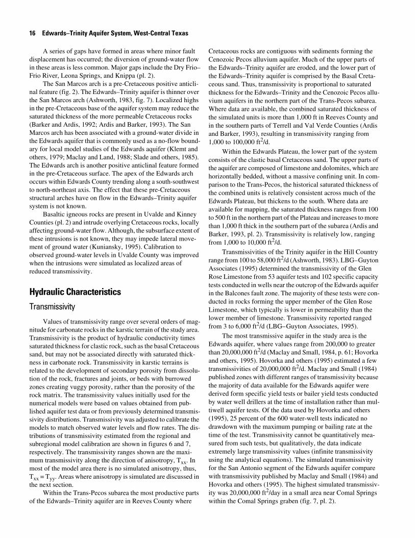
16 Edwards–Trinity Aquifer System, West-Central Texas
A series of gaps have formed in areas where minor fault displacement has occurred; the diversion of ground-water flow in these areas is less common. Major gaps include the Dry Frio–Frio River, Leona Springs, and Knippa (pl. 2).
The San Marcos arch is a pre-Cretaceous positive anticli-nal feature (fig. 2). The Edwards–Trinity aquifer is thinner over the San Marcos arch (Ashworth, 1983, fig. 7). Localized highs in the pre-Cretaceous base of the aquifer system may reduce the saturated thickness of the more permeable Cretaceous rocks (Barker and Ardis, 1992; Ardis and Barker, 1993). The San Marcos arch has been associated with a ground-water divide in the Edwards aquifer that is commonly used as a no-flow bound-ary for local model studies of the Edwards aquifer (Klemt and others, 1979; Maclay and Land, 1988; Slade and others, 1985). The Edwards arch is another positive anticlinal feature formed in the pre-Cretaceous surface. The apex of the Edwards arch occurs within Edwards County trending along a south-southwest to north-northeast axis. The effect that these pre-Cretaceous structural arches have on flow in the Edwards–Trinity aquifer system is not known.
Basaltic igneous rocks are present in Uvalde and Kinney Counties (pl. 2) and intrude overlying Cretaceous rocks, locally affecting ground-water flow. Although, the subsurface extent of these intrusions is not known, they may impede lateral move-ment of ground water (Kuniansky, 1995). Calibration to observed ground-water levels in Uvalde County was improved when the intrusions were simulated as localized areas of reduced transmissivity.
Hydraulic CharacteristicsTransmissivity
Values of transmissivity range over several orders of mag-nitude for carbonate rocks in the karstic terrain of the study area. Transmissivity is the product of hydraulic conductivity times saturated thickness for clastic rock, such as the basal Cretaceous sand, but may not be associated directly with saturated thick-ness in carbonate rock. Transmissivity in karstic terrains is related to the development of secondary porosity from dissolu-tion of the rock, fractures and joints, or beds with burrowed zones creating vuggy porosity, rather than the porosity of the rock matrix. The transmissivity values initially used for the numerical models were based on values obtained from pub-lished aquifer test data or from previously determined transmis-sivity distributions. Transmissivity was adjusted to calibrate the models to match observed water levels and flow rates. The dis-tributions of transmissivity estimated from the regional and subregional model calibration are shown in figures 6 and 7, respectively. The transmissivity ranges shown are the maxi-mum transmissivity along the direction of anisotropy, Txx. In most of the model area there is no simulated anisotropy, thus, Txx = Tyy. Areas where anisotropy is simulated are discussed in the next section.
Within the Trans-Pecos subarea the most productive parts of the Edwards–Trinity aquifer are in Reeves County where
Cretaceous rocks are contiguous with sediments forming the Cenozoic Pecos alluvium aquifer. Much of the upper parts of the Edwards–Trinity aquifer are eroded, and the lower part of the Edwards–Trinity aquifer is comprised by the Basal Creta-ceous sand. Thus, transmissivity is proportional to saturated thickness for the Edwards–Trinity and the Cenozoic Pecos allu-vium aquifers in the northern part of the Trans-Pecos subarea. Where data are available, the combined saturated thickness of the simulated units is more than 1,000 ft in Reeves County and in the southern parts of Terrell and Val Verde Counties (Ardis and Barker, 1993), resulting in transmissivity ranging from 1,000 to 100,000 ft2/d.
Within the Edwards Plateau, the lower part of the system consists of the clastic basal Cretaceous sand. The upper parts of the aquifer are composed of limestone and dolomites, which are horizontally bedded, without a massive confining unit. In com-parison to the Trans-Pecos, the historical saturated thickness of the combined units is relatively consistent across much of the Edwards Plateau, but thickens to the south. Where data are available for mapping, the saturated thickness ranges from 100 to 500 ft in the northern part of the Plateau and increases to more than 1,000 ft thick in the southern part of the subarea (Ardis and Barker, 1993, pl. 2). Transmissivity is relatively low, ranging from 1,000 to 10,000 ft2/d.
Transmissivities of the Trinity aquifer in the Hill Country range from 100 to 58,000 ft2/d (Ashworth, 1983). LBG–Guyton Associates (1995) determined the transmissivity of the Glen Rose Limestone from 53 aquifer tests and 102 specific capacity tests conducted in wells near the outcrop of the Edwards aquifer in the Balcones fault zone. The majority of these tests were con-ducted in rocks forming the upper member of the Glen Rose Limestone, which typically is lower in permeability than the lower member of limestone. Transmissivity reported ranged from 3 to 6,000 ft2/d (LBG–Guyton Associates, 1995).
The most transmissive aquifer in the study area is the Edwards aquifer, where values range from 200,000 to greater than 20,000,000 ft2/d (Maclay and Small, 1984, p. 61; Hovorka and others, 1995). Hovorka and others (1995) estimated a few transmissivities of 20,000,000 ft2/d. Maclay and Small (1984) published zones with different ranges of transmissivity because the majority of data available for the Edwards aquifer were derived form specific yield tests or bailer yield tests conducted by water well drillers at the time of installation rather than mul-tiwell aquifer tests. Of the data used by Hovorka and others (1995), 25 percent of the 600 water-well tests indicated no drawdown with the maximum pumping or bailing rate at the time of the test. Transmissivity cannot be quantitatively mea-sured from such tests, but qualitatively, the data indicate extremely large transmissivity values (infinite transmissivity using the analytical equations). The simulated transmissivity for the San Antonio segment of the Edwards aquifer compare with transmissivity published by Maclay and Small (1984) and Hovorka and others (1995). The highest simulated transmissiv-ity was 20,000,000 ft2/day in a small area near Comal Springs within the Comal Springs graben (fig. 7, pl. 2).
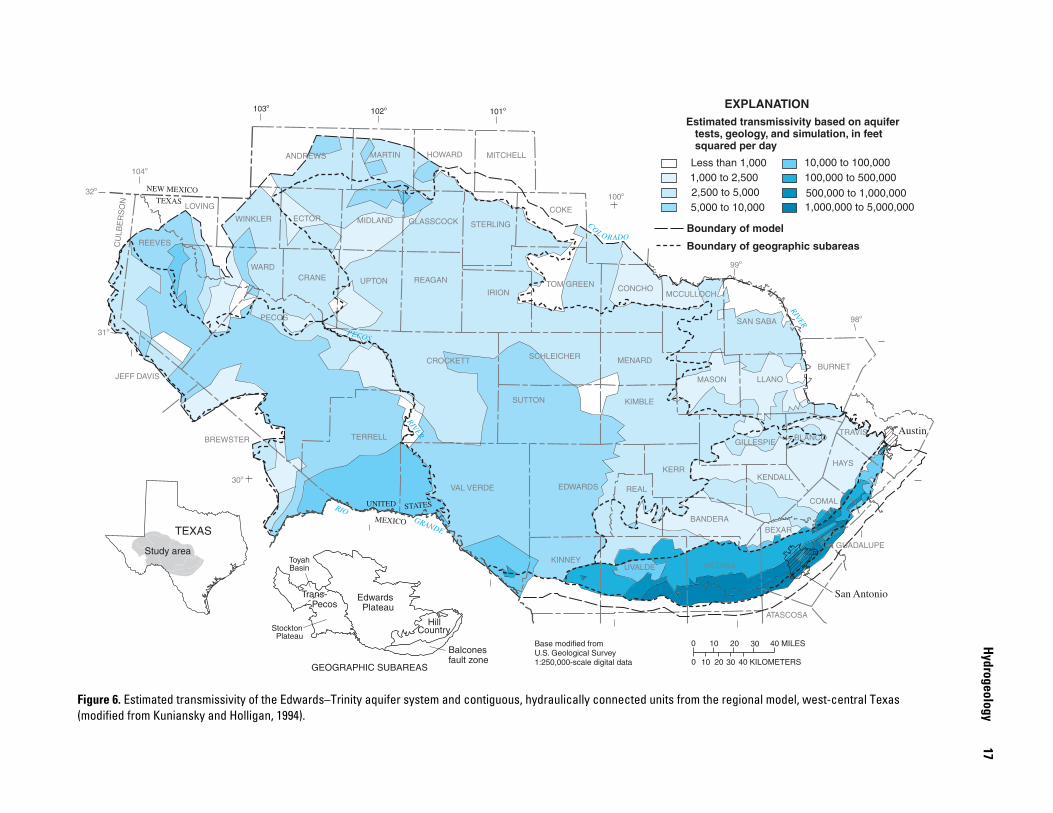
Hydrogeology
17
Figure 6. Estimated transmissivity of the Edwards–Trinity aquifer system and contiguous, hydraulically connected units from the regional model, west-central Texas (modified from Kuniansky and Holligan, 1994).
0 10 20 30 40 MILES
0 10 20 30 40 KILOMETERS
GRANDE
RIO
PECOS
RIVER
COL ORADO
RIVER
Estimated transmissivity based on aquifer tests, geology, and simulation, in feet squared per day
EXPLANATION
Less than 1,0001,000 to 2,5002,500 to 5,0005,000 to 10,000
10,000 to 100,000100,000 to 500,000
500,000 to 1,000,0001,000,000 to 5,000,000
Boundary of model
Boundary of geographic subareas
Austin
San Antonio
Base modified from U.S. Geological Survey1:250,000-scale digital data
98o
99o
100o
104o
32o
31o
30o
ANDREWS MARTIN HOWARD
LOVING
WINKLER ECTOR
REEVES
WARD
CU
LBE
RS
ON
STERLING
IRION
REAGANUPTON
GLASSCOCKMIDLAND
PECOS
CRANE
JEFF DAVIS
BREWSTER TERRELL
CROCKETT
NEW MEXICOTEXAS
UNITED
MEXICO
STATES
MITCHELL
COKE
MASON
TOM GREEN CONCHOMCCULLOCH
SAN SABA
LLANO
BURNET
GILLESPIEBLANCO
TRAVIS
KERR
BANDERA
KENDALL
HAYS
BEXAR
GUADALUPE
COMAL
ATASCOSA
MEDINA
EDWARDS REAL
UVALDEKINNEY
VAL VERDE
SCHLEICHER MENARD
KIMBLESUTTON
101o102o103o
TEXAS
Study area
Edwards Plateau
Trans- Pecos
Hill Country
Balconesfault zone
GEOGRAPHIC SUBAREAS
ToyahBasin
Stockton Plateau
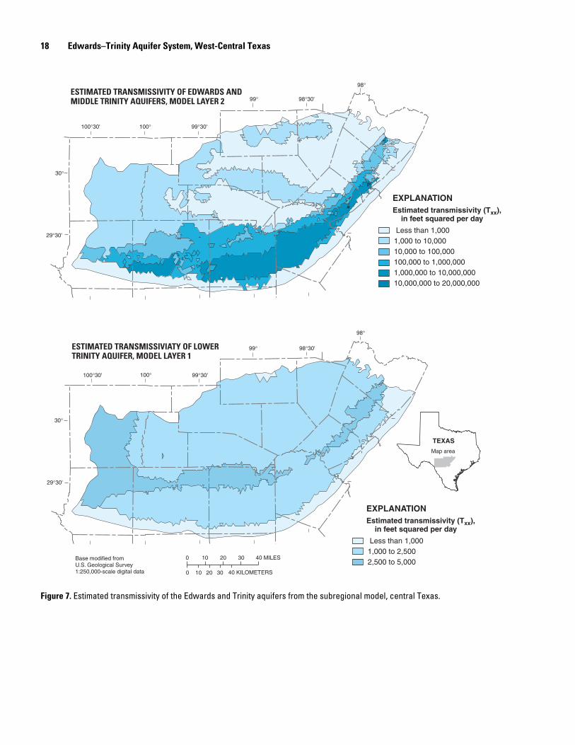
18 Edwards–Trinity Aquifer System, West-Central Texas
Figure 7. Estimated transmissivity of the Edwards and Trinity aquifers from the subregional model, central Texas.
0 10 20 30
0 10 20 30
ESTIMATED TRANSMISSIVIATY OF LOWER TRINITY AQUIFER, MODEL LAYER 1
ESTIMATED TRANSMISSIVITY OF EDWARDS AND MIDDLE TRINITY AQUIFERS, MODEL LAYER 2
40 MILES
40 KILOMETERS
Estimated transmissivity (Txx), in feet squared per day
EXPLANATION
Less than 1,0001,000 to 10,00010,000 to 100,000100,000 to 1,000,0001,000,000 to 10,000,00010,000,000 to 20,000,000
Estimated transmissivity (Txx), in feet squared per day
EXPLANATION
Less than 1,0001,000 to 2,5002,500 to 5,000
98°30'99°
98°
99°30'100°100°30'
29°30'
30°
99°30'100°100°30'
29°30'
30°
98°30'99°
98°
Base modified from U.S. Geological Survey1:250,000-scale digital data
TEXAS
Map area
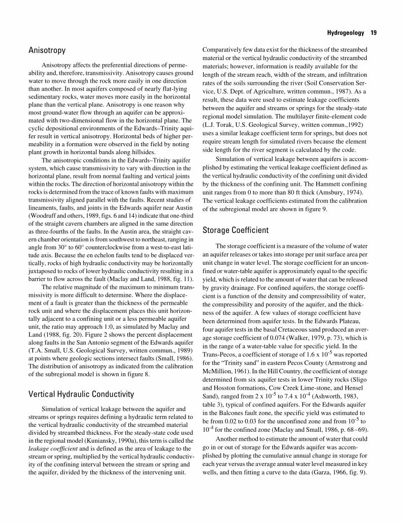
Hydrogeology 19
Anisotropy
Anisotropy affects the preferential directions of perme-ability and, therefore, transmissivity. Anisotropy causes ground water to move through the rock more easily in one direction than another. In most aquifers composed of nearly flat-lying sedimentary rocks, water moves more easily in the horizontal plane than the vertical plane. Anisotropy is one reason why most ground-water flow through an aquifer can be approxi-mated with two-dimensional flow in the horizontal plane. The cyclic depositional environments of the Edwards–Trinity aqui-fer result in vertical anisotropy. Horizontal beds of higher per-meability in a formation were observed in the field by noting plant growth in horizontal bands along hillsides.
The anisotropic conditions in the Edwards–Trinity aquifer system, which cause transmissivity to vary with direction in the horizontal plane, result from normal faulting and vertical joints within the rocks. The direction of horizontal anisotropy within the rocks is determined from the trace of known faults with maximum transmissivity aligned parallel with the faults. Recent studies of lineaments, faults, and joints in the Edwards aquifer near Austin (Woodruff and others, 1989, figs. 6 and 14) indicate that one-third of the straight cavern chambers are aligned in the same direction as three-fourths of the faults. In the Austin area, the straight cav-ern chamber orientation is from southwest to northeast, ranging in angle from 30° to 60° counterclockwise from a west-to-east lati-tude axis. Because the en echelon faults tend to be displaced ver-tically, rocks of high hydraulic conductivity may be horizontally juxtaposed to rocks of lower hydraulic conductivity resulting in a barrier to flow across the fault (Maclay and Land, 1988, fig. 11).
The relative magnitude of the maximum to minimum trans-missivity is more difficult to determine. Where the displace-ment of a fault is greater than the thickness of the permeable rock unit and where the displacement places this unit horizon-tally adjacent to a confining unit or a less permeable aquifer unit, the ratio may approach 1:0, as simulated by Maclay and Land (1988, fig. 20). Figure 2 shows the percent displacement along faults in the San Antonio segment of the Edwards aquifer (T.A. Small, U.S. Geological Survey, written commun., 1989) at points where geologic sections intersect faults (Small, 1986). The distribution of anisotropy as indicated from the calibration of the subregional model is shown in figure 8.
Vertical Hydraulic Conductivity
Simulation of vertical leakage between the aquifer and streams or springs requires defining a hydraulic term related to the vertical hydraulic conductivity of the streambed material divided by streambed thickness. For the steady-state code used in the regional model (Kuniansky, 1990a), this term is called the leakage coefficient and is defined as the area of leakage to the stream or spring, multiplied by the vertical hydraulic conductiv-ity of the confining interval between the stream or spring and the aquifer, divided by the thickness of the intervening unit.
Comparatively few data exist for the thickness of the streambed material or the vertical hydraulic conductivity of the streambed materials; however, information is readily available for the length of the stream reach, width of the stream, and infiltration rates of the soils surrounding the river (Soil Conservation Ser-vice, U.S. Dept. of Agriculture, written commun., 1987). As a result, these data were used to estimate leakage coefficients between the aquifer and streams or springs for the steady-state regional model simulation. The multilayer finite-element code (L.J. Torak, U.S. Geological Survey, written commun.,1992) uses a similar leakage coefficient term for springs, but does not require stream length for simulated rivers because the element side length for the river segment is calculated by the code.
Simulation of vertical leakage between aquifers is accom-plished by estimating the vertical leakage coefficient defined as the vertical hydraulic conductivity of the confining unit divided by the thickness of the confining unit. The Hammett confining unit ranges from 0 to more than 80 ft thick (Amsbury, 1974). The vertical leakage coefficients estimated from the calibration of the subregional model are shown in figure 9.
Storage Coefficient
The storage coefficient is a measure of the volume of water an aquifer releases or takes into storage per unit surface area per unit change in water level. The storage coefficient for an uncon-fined or water-table aquifer is approximately equal to the specific yield, which is related to the amount of water that can be released by gravity drainage. For confined aquifers, the storage coeffi-cient is a function of the density and compressibility of water, the compressibility and porosity of the aquifer, and the thick-ness of the aquifer. A few values of storage coefficient have been determined from aquifer tests. In the Edwards Plateau, four aquifer tests in the basal Cretaceous sand produced an aver-age storage coefficient of 0.074 (Walker, 1979, p. 73), which is in the range of a water-table value for specific yield. In the Trans-Pecos, a coefficient of storage of 1.6 x 10⁻⁵ was reported for the “Trinity sand” in eastern Pecos County (Armstrong and McMillion, 1961). In the Hill Country, the coefficient of storage determined from six aquifer tests in lower Trinity rocks (Sligo and Hosston formations, Cow Creek Lime-stone, and Hensel Sand), ranged from 2 x 10⁻⁵ to 7.4 x 10⁻⁴ (Ashworth, 1983, table 3), typical of confined aquifers. For the Edwards aquifer in the Balcones fault zone, the specific yield was estimated to be from 0.02 to 0.03 for the unconfined zone and from 10-5 to 10-4 for the confined zone (Maclay and Small, 1986, p. 68–69).
Another method to estimate the amount of water that could go in or out of storage for the Edwards aquifer was accom-plished by plotting the cumulative annual change in storage for each year versus the average annual water level measured in key wells, and then fitting a curve to the data (Garza, 1966, fig. 9).
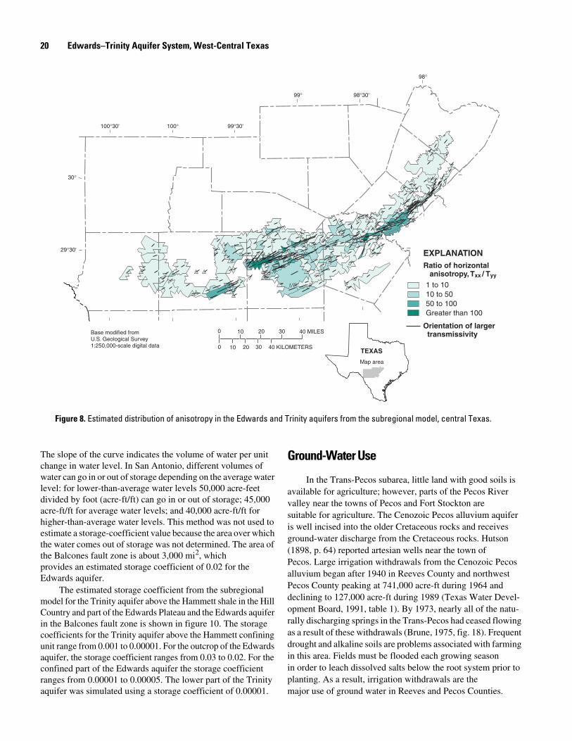
20 Edwards–Trinity Aquifer System, West-Central Texas
Figure 8. Estimated distribution of anisotropy in the Edwards and Trinity aquifers from the subregional model, central Texas.
98°
99° 98°30'
99°30'100°30'
29°30'
30°
100°
0 10 20 30 40 MILES
0 10 20 30 40 KILOMETERS
1 to 1010 to 5050 to 100Greater than 100
Orientation of larger transmissivity
Ratio of horizontal anisotropy, Txx / Tyy
EXPLANATION
Base modified from U.S. Geological Survey1:250,000-scale digital data
TEXAS
Map area
The slope of the curve indicates the volume of water per unit change in water level. In San Antonio, different volumes of water can go in or out of storage depending on the average water level: for lower-than-average water levels 50,000 acre-feet divided by foot (acre-ft/ft) can go in or out of storage; 45,000 acre-ft/ft for average water levels; and 40,000 acre-ft/ft for higher-than-average water levels. This method was not used to estimate a storage-coefficient value because the area over which the water comes out of storage was not determined. The area of the Balcones fault zone is about 3,000 mi2, which provides an estimated storage coefficient of 0.02 for the Edwards aquifer.
The estimated storage coefficient from the subregional model for the Trinity aquifer above the Hammett shale in the Hill Country and part of the Edwards Plateau and the Edwards aquifer in the Balcones fault zone is shown in figure 10. The storage coefficients for the Trinity aquifer above the Hammett confining unit range from 0.001 to 0.00001. For the outcrop of the Edwards aquifer, the storage coefficient ranges from 0.03 to 0.02. For the confined part of the Edwards aquifer the storage coefficient ranges from 0.00001 to 0.00005. The lower part of the Trinity aquifer was simulated using a storage coefficient of 0.00001.
Ground-Water Use
In the Trans-Pecos subarea, little land with good soils is available for agriculture; however, parts of the Pecos River valley near the towns of Pecos and Fort Stockton are suitable for agriculture. The Cenozoic Pecos alluvium aquifer is well incised into the older Cretaceous rocks and receives ground-water discharge from the Cretaceous rocks. Hutson (1898, p. 64) reported artesian wells near the town of Pecos. Large irrigation withdrawals from the Cenozoic Pecos alluvium began after 1940 in Reeves County and northwest Pecos County peaking at 741,000 acre-ft during 1964 and declining to 127,000 acre-ft during 1989 (Texas Water Devel-opment Board, 1991, table 1). By 1973, nearly all of the natu-rally discharging springs in the Trans-Pecos had ceased flowing as a result of these withdrawals (Brune, 1975, fig. 18). Frequent drought and alkaline soils are problems associated with farming in this area. Fields must be flooded each growing season in order to leach dissolved salts below the root system prior to planting. As a result, irrigation withdrawals are the major use of ground water in Reeves and Pecos Counties.
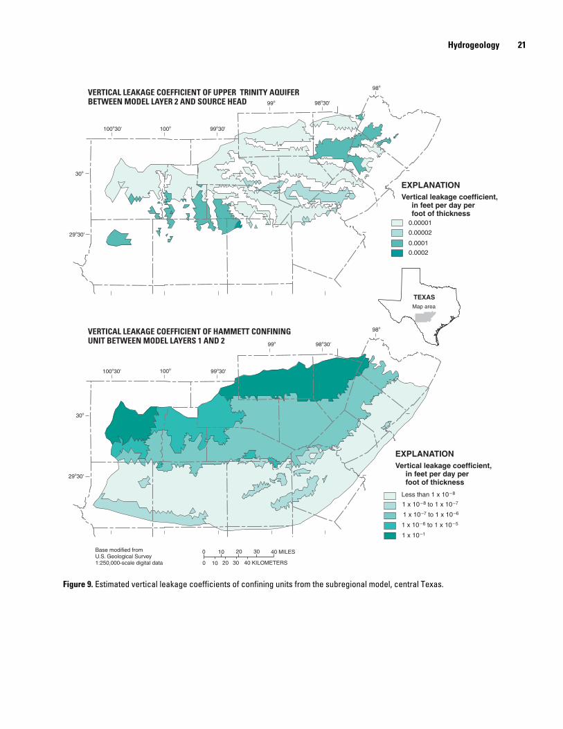
Hydrogeology 21
Figure 9. Estimated vertical leakage coefficients of confining units from the subregional model, central Texas.
0 10 20 30 40 MILES
0 10 20 30 40 KILOMETERS
VERTICAL LEAKAGE COEFFICIENT OF UPPER TRINITY AQUIFERBETWEEN MODEL LAYER 2 AND SOURCE HEAD
VERTICAL LEAKAGE COEFFICIENT OF HAMMETT CONFININGUNIT BETWEEN MODEL LAYERS 1 AND 2
1 x 10⁻⁸ to 1 x 10⁻⁷
1 x 10⁻¹
1 x 10⁻⁶ to 1 x 10⁻⁵
1 x 10⁻⁷ to 1 x 10⁻⁶
Less than 1 x 10⁻⁸
0.00002
0.0001
0.0002
0.00001
Vertical leakage coefficient, in feet per day per foot of thickness
EXPLANATION
Vertical leakage coefficient, in feet per day per foot of thickness
EXPLANATION
Base modified from U.S. Geological Survey1:250,000-scale digital data
98o
98o30'99o
99o30'100o100o30'
29o30'
30o
98o30'99o
98o
99o30'100o100o30'
29o30'
30o
TEXASMap area
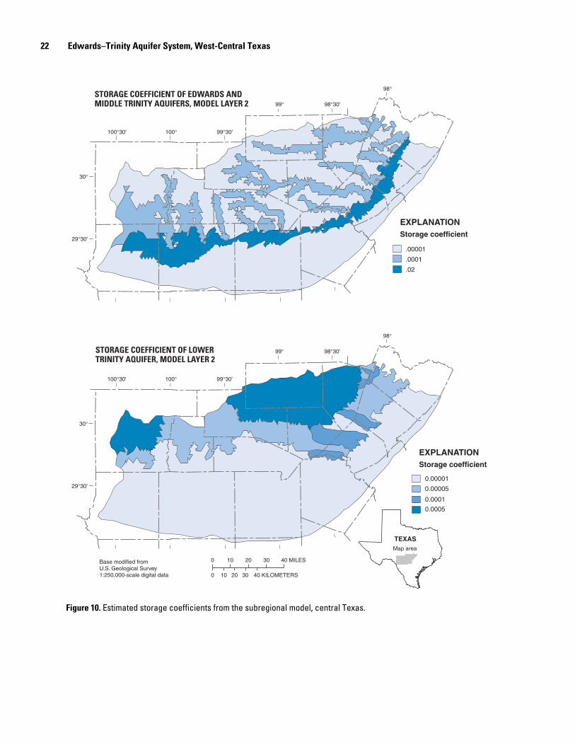
22 Edwards–Trinity Aquifer System, West-Central Texas
Figure 10. Estimated storage coefficients from the subregional model, central Texas.
98°30'99°
29°30'
30°
98°
99°30'100°100°30'
98°30'99°
29°30'
30°
98°
99°30'100°100°30'
STORAGE COEFFICIENT OF EDWARDS ANDMIDDLE TRINITY AQUIFERS, MODEL LAYER 2
STORAGE COEFFICIENT OF LOWER TRINITY AQUIFER, MODEL LAYER 2
TEXASMap area
Base modified from U.S. Geological Survey1:250,000-scale digital data
0.00005
0.0001
0.0005
0.00001
Storage coefficient
EXPLANATION
Storage coefficient
EXPLANATION
.0001
.02
.00001
0 10 20 30 40 MILES
0 10 20 30 40 KILOMETERS
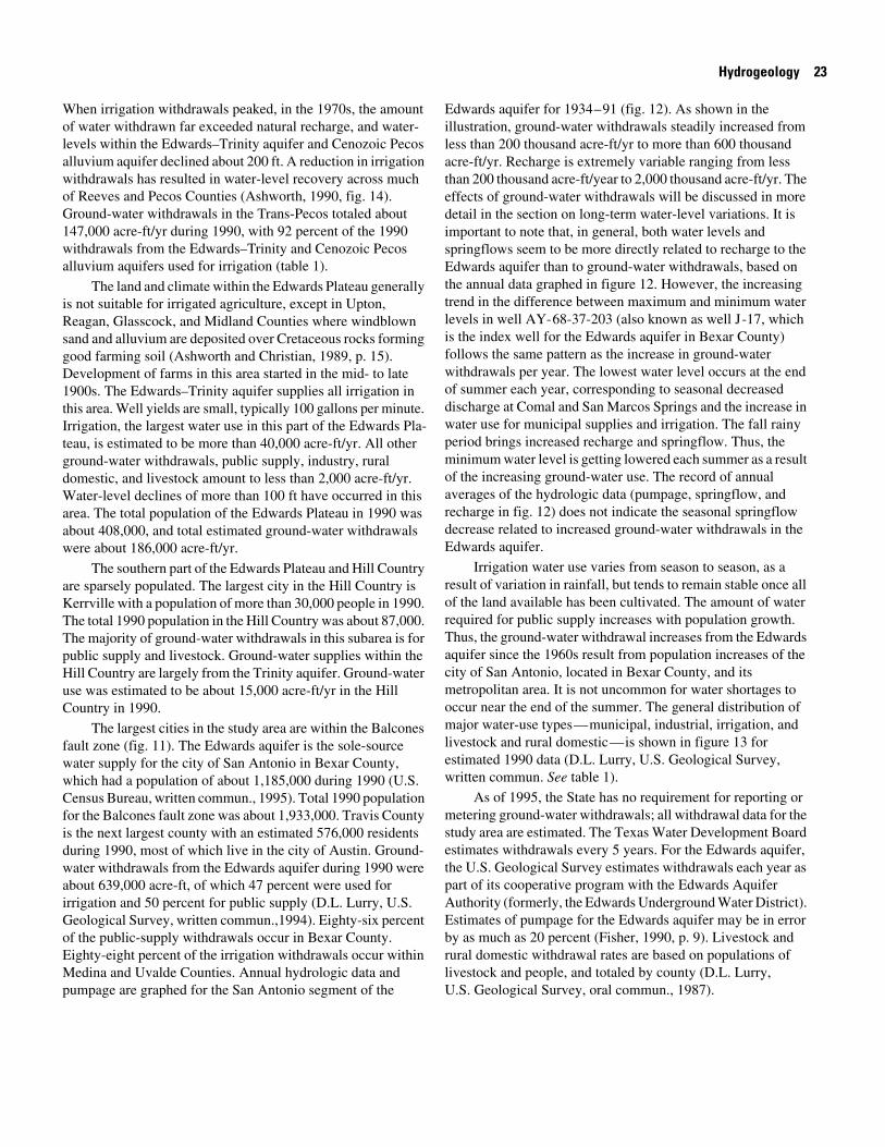
Hydrogeology 23
When irrigation withdrawals peaked, in the 1970s, the amount of water withdrawn far exceeded natural recharge, and water-levels within the Edwards–Trinity aquifer and Cenozoic Pecos alluvium aquifer declined about 200 ft. A reduction in irrigation withdrawals has resulted in water-level recovery across much of Reeves and Pecos Counties (Ashworth, 1990, fig. 14). Ground-water withdrawals in the Trans-Pecos totaled about 147,000 acre-ft/yr during 1990, with 92 percent of the 1990 withdrawals from the Edwards–Trinity and Cenozoic Pecos alluvium aquifers used for irrigation (table 1).
The land and climate within the Edwards Plateau generally is not suitable for irrigated agriculture, except in Upton, Reagan, Glasscock, and Midland Counties where windblown sand and alluvium are deposited over Cretaceous rocks forming good farming soil (Ashworth and Christian, 1989, p. 15). Development of farms in this area started in the mid- to late 1900s. The Edwards–Trinity aquifer supplies all irrigation in this area. Well yields are small, typically 100 gallons per minute. Irrigation, the largest water use in this part of the Edwards Pla-teau, is estimated to be more than 40,000 acre-ft/yr. All other ground-water withdrawals, public supply, industry, rural domestic, and livestock amount to less than 2,000 acre-ft/yr. Water-level declines of more than 100 ft have occurred in this area. The total population of the Edwards Plateau in 1990 was about 408,000, and total estimated ground-water withdrawals were about 186,000 acre-ft/yr.
The southern part of the Edwards Plateau and Hill Country are sparsely populated. The largest city in the Hill Country is Kerrville with a population of more than 30,000 people in 1990. The total 1990 population in the Hill Country was about 87,000. The majority of ground-water withdrawals in this subarea is for public supply and livestock. Ground-water supplies within the Hill Country are largely from the Trinity aquifer. Ground-water use was estimated to be about 15,000 acre-ft/yr in the Hill Country in 1990.
The largest cities in the study area are within the Balcones fault zone (fig. 11). The Edwards aquifer is the sole-source water supply for the city of San Antonio in Bexar County, which had a population of about 1,185,000 during 1990 (U.S. Census Bureau, written commun., 1995). Total 1990 population for the Balcones fault zone was about 1,933,000. Travis County is the next largest county with an estimated 576,000 residents during 1990, most of which live in the city of Austin. Ground-water withdrawals from the Edwards aquifer during 1990 were about 639,000 acre-ft, of which 47 percent were used for irrigation and 50 percent for public supply (D.L. Lurry, U.S. Geological Survey, written commun.,1994). Eighty-six percent of the public-supply withdrawals occur in Bexar County. Eighty-eight percent of the irrigation withdrawals occur within Medina and Uvalde Counties. Annual hydrologic data and pumpage are graphed for the San Antonio segment of the
Edwards aquifer for 1934–91 (fig. 12). As shown in the illustration, ground-water withdrawals steadily increased from less than 200 thousand acre-ft/yr to more than 600 thousand acre-ft/yr. Recharge is extremely variable ranging from less than 200 thousand acre-ft/year to 2,000 thousand acre-ft/yr. The effects of ground-water withdrawals will be discussed in more detail in the section on long-term water-level variations. It is important to note that, in general, both water levels and springflows seem to be more directly related to recharge to the Edwards aquifer than to ground-water withdrawals, based on the annual data graphed in figure 12. However, the increasing trend in the difference between maximum and minimum water levels in well AY-68-37-203 (also known as well J-17, which is the index well for the Edwards aquifer in Bexar County) follows the same pattern as the increase in ground-water withdrawals per year. The lowest water level occurs at the end of summer each year, corresponding to seasonal decreased discharge at Comal and San Marcos Springs and the increase in water use for municipal supplies and irrigation. The fall rainy period brings increased recharge and springflow. Thus, the minimum water level is getting lowered each summer as a result of the increasing ground-water use. The record of annual averages of the hydrologic data (pumpage, springflow, and recharge in fig. 12) does not indicate the seasonal springflow decrease related to increased ground-water withdrawals in the Edwards aquifer.
Irrigation water use varies from season to season, as a result of variation in rainfall, but tends to remain stable once all of the land available has been cultivated. The amount of water required for public supply increases with population growth. Thus, the ground-water withdrawal increases from the Edwards aquifer since the 1960s result from population increases of the city of San Antonio, located in Bexar County, and its metropolitan area. It is not uncommon for water shortages to occur near the end of the summer. The general distribution of major water-use types—municipal, industrial, irrigation, and livestock and rural domestic—is shown in figure 13 for estimated 1990 data (D.L. Lurry, U.S. Geological Survey, written commun. See table 1).
As of 1995, the State has no requirement for reporting or metering ground-water withdrawals; all withdrawal data for the study area are estimated. The Texas Water Development Board estimates withdrawals every 5 years. For the Edwards aquifer, the U.S. Geological Survey estimates withdrawals each year as part of its cooperative program with the Edwards Aquifer Authority (formerly, the Edwards Underground Water District). Estimates of pumpage for the Edwards aquifer may be in error by as much as 20 percent (Fisher, 1990, p. 9). Livestock and rural domestic withdrawal rates are based on populations of livestock and people, and totaled by county (D.L. Lurry, U.S. Geological Survey, oral commun., 1987).
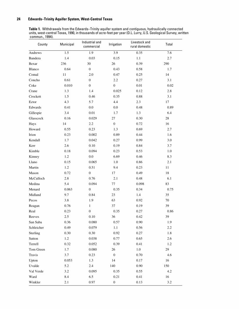
24 Edwards–Trinity Aquifer System, West-Central Texas
Table 1. Withdrawals from the Edwards–Trinity aquifer system and contiguous, hydraulically connected units, west-central Texas, 1990, in thousands of acre-feet per year (D.L. Lurry, U.S. Geological Survey, written commun., 1994).
County Municipal Industrial and commercial Irrigation Livestock and
rural domestic Total
Andrews 1.5 1.9 3.9 0.35 7.6
Bandera 1.4 0.03 0.15 1.1 2.7
Bexar 236 30 26 0.39 290
Blanco 0.64 0 0.43 0.58 1.7
Comal 11 2.0 0.47 0.25 14
Concho 0.61 0 2.2 0.27 3.1
Coke 0.010 0 0 0.01 0.02
Crane 1.3 1.4 0.025 0.12 2.8
Crockett 1.5 0.46 0.35 0.88 3.1
Ector 4.3 5.7 4.4 2.3 17
Edwards 0.41 0.0 0.0 0.48 0.89
Gillespie 3.4 0.01 1.7 1.3 6.4
Glasscock 0.16 0.029 27 0.30 28
Hays 14 2.2 0 0.72 16
Howard 0.55 0.23 1.3 0.69 2.7
Irion 0.23 0.002 0.89 0.44 1.6
Kendall 1.7 0.042 0.27 0.99 3.0
Kerr 2.6 0.10 0.19 0.84 3.7
Kimble 0.18 0.094 0.23 0.53 1.0
Kinney 1.2 0.0 6.69 0.46 8.3
Llano 0.15 0.065 1.0 0.86 2.1
Martin 1.2 0.51 9.4 0.23 11
Mason 0.72 0 17 0.49 18
McCulloch 2.8 0.76 2.1 0.48 6.1
Medina 5.4 0.094 77 0.098 83
Menard 0.063 0 0.35 0.34 0.75
Midland 9.7 0.84 23 1.4 35
Pecos 3.8 1.9 63 0.92 70
Reagan 0.76 1 37 0.19 39
Real 0.23 0 0.35 0.27 0.86
Reeves 2.5 0.10 36 0.42 39
San Saba 0.36 0.080 0.57 0.90 1.9
Schleicher 0.49 0.079 1.1 0.56 2.2
Sterling 0.30 0.30 0.92 0.27 1.8
Sutton 1.2 0.038 0.77 0.65 2.6
Terrell 0.32 0.052 0.39 0.41 1.2
Tom Green 1.7 0.080 26 1.0 29
Travis 3.7 0.23 0 0.70 4.6
Upton 0.053 1.3 14 0.17 16
Uvalde 5.2 2.4 140 0.90 150
Val Verde 3.2 0.095 0.35 0.55 4.2
Ward 8.4 6.5 0.21 0.41 16
Winkler 2.1 0.97 0 0.13 3.2
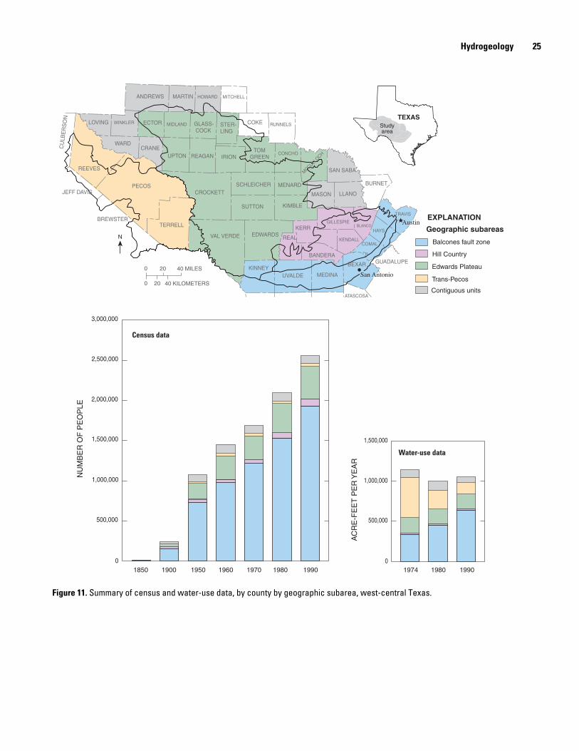
Hydrogeology 25
Figure 11. Summary of census and water-use data, by county by geographic subarea, west-central Texas.
ANDREWS MARTIN HOWARD MITCHELL
CU
LBE
RS
ON
LOVING
REEVES
WARD
PECOS
WINKLER ECTOR
CRANE
MIDLAND GLASS- COCK
UPTON REAGAN
STER-LING
COKE
IRIONTOM
GREENCONCHO
RUNNELS
MCCULLOCH
SAN SABA
JEFF DAVIS
BREWSTERTERRELL
VAL VERDE
CROCKETTSCHLEICHER
SUTTON
EDWARDS
KINNEYUVALDE
MENARD
REAL
KERR
BANDERA
MEDINA
ATASCOSA
BEXAR
KENDALLCOMAL
GUADALUPE
GILLESPIE
MASON LLANO
BURNET
BLANCO
TRAVIS
HAYS
KIMBLE
Contiguous units
Trans-Pecos
Edwards Plateau
Hill Country
Balcones fault zone
Geographic subareas
EXPLANATION
0 20 40 MILES
0 20 40 KILOMETERS
N
3,000,000
2,500,000
2,000,000
1,500,000
1,000,000
500,000
0
NU
MB
ER
OF
PE
OP
LE
1,500,000
1,000,000
500,000
0
AC
RE
-FE
ET
PE
R Y
EA
R
1850 1900 1950 1960 1970 1980 1990 1974 1980 1990
Census data
Water-use data
Austin
San Antonio
TEXASStudy area
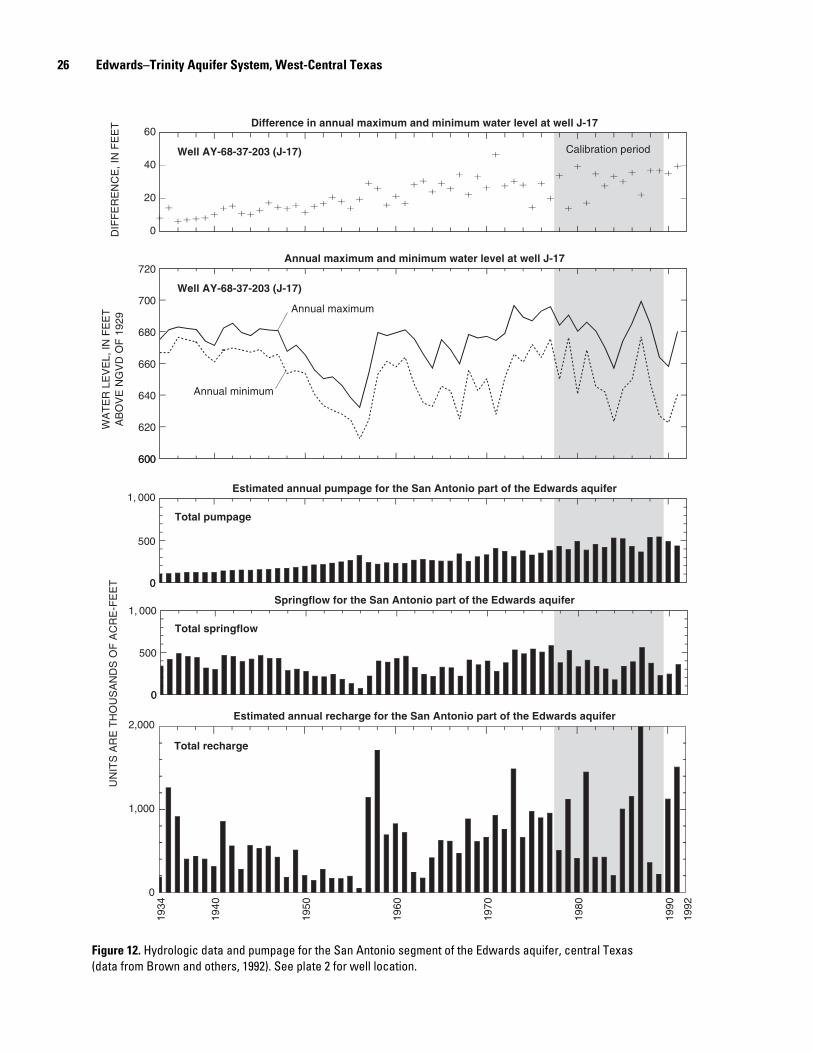
26 Edwards–Trinity Aquifer System, West-Central Texas
Figure 12. Hydrologic data and pumpage for the San Antonio segment of the Edwards aquifer, central Texas (data from Brown and others, 1992). See plate 2 for well location.
0
60
20
40
DIF
FE
RE
NC
E, I
N F
EE
T
Well AY-68-37-203 (J-17)
Well AY-68-37-203 (J-17)
600
720
600
620
640
660
680
700
WA
TE
R L
EV
EL,
IN F
EE
TA
BO
VE
NG
VD
OF
192
9 Annual maximum
Annual minimum
0
1, 000
0
500
Total pumpage
Total springflow
Total recharge
0
1, 000
0
500
1934
1992
1940
1950
1960
1970
1980
1990
UN
ITS
AR
E T
HO
US
AN
DS
OF
AC
RE
-FE
ET
Difference in annual maximum and minimum water level at well J-17
Annual maximum and minimum water level at well J-17
Estimated annual pumpage for the San Antonio part of the Edwards aquifer
Springflow for the San Antonio part of the Edwards aquifer
Estimated annual recharge for the San Antonio part of the Edwards aquifer2,000
1,000
0
Calibration period
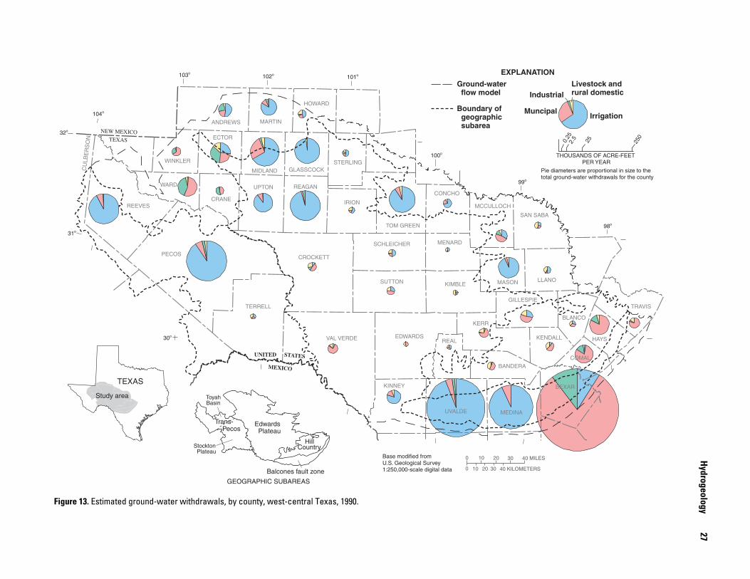
Hydrogeology
27
Figure 13. Estimated ground-water withdrawals, by county, west-central Texas, 1990.
98o
99o
100o
101o102o103o
104o
32o
31o
30o
ANDREWS MARTIN
HOWARD
WINKLER
ECTOR
REEVES
WARD
CU
LBE
RS
ON
STERLING
IRION
REAGANUPTON
GLASSCOCKMIDLAND
PECOS
CRANE
TERRELL
CROCKETT
NEW MEXICOTEXAS
UNITED
MEXICO
STATES
MASON
TOM GREEN
CONCHO
MCCULLOCH
SAN SABA
LLANO
GILLESPIE
BLANCO
TRAVIS
KERR
BANDERA
KENDALL HAYS
BEXAR
COMAL
MEDINA
EDWARDSREAL
UVALDE
KINNEY
VAL VERDE
SCHLEICHER MENARD
KIMBLESUTTON
0 10 20 30 40 MILES
0 10 20 30 40 KILOMETERS
Base modified from U.S. Geological Survey1:250,000-scale digital data
IrrigationMuncipal
IndustrialLivestock and rural domestic
EXPLANATION
0.25
2.5 25 250
THOUSANDS OF ACRE-FEET PER YEAR
Pie diameters are proportional in size to the total ground-water withdrawals for the county
Ground-water flow model
Boundary of geographic subarea
TEXAS
Study area
Edwards Plateau
Trans- Pecos
Hill Country
Balcones fault zone
GEOGRAPHIC SUBAREAS
ToyahBasin
Stockton Plateau
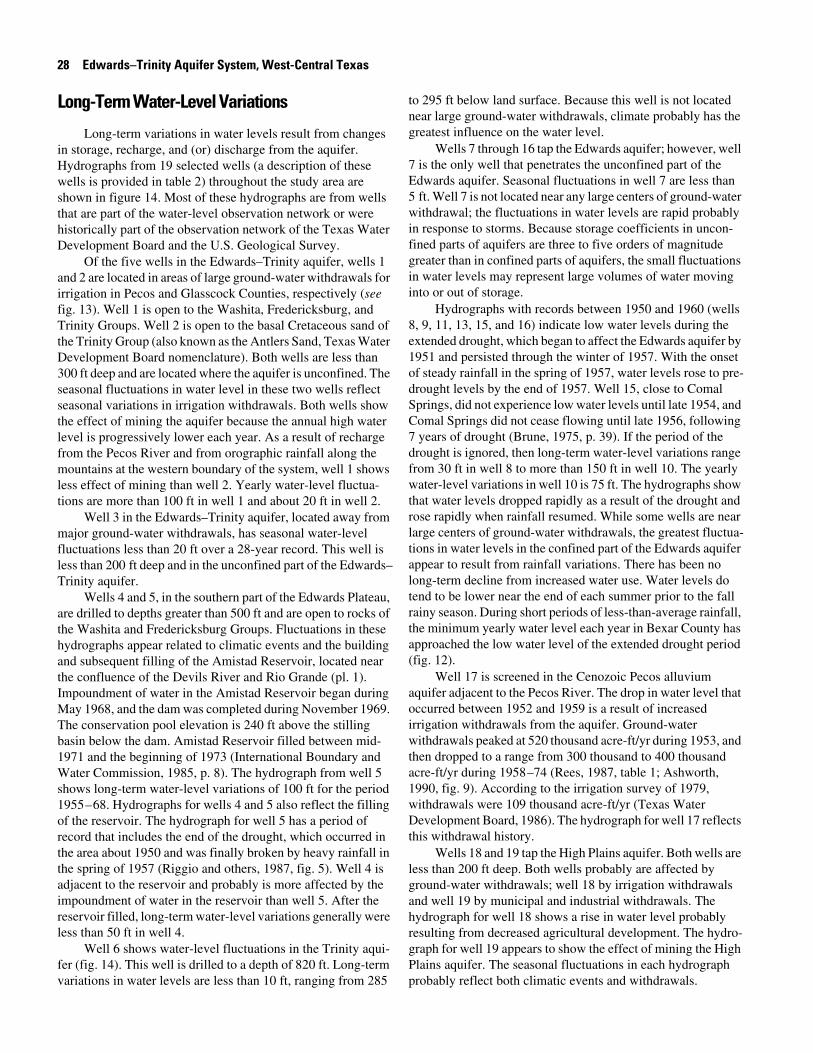
28 Edwards–Trinity Aquifer System, West-Central Texas
Long-Term Water-Level Variations
Long-term variations in water levels result from changes in storage, recharge, and (or) discharge from the aquifer. Hydrographs from 19 selected wells (a description of these wells is provided in table 2) throughout the study area are shown in figure 14. Most of these hydrographs are from wells that are part of the water-level observation network or were historically part of the observation network of the Texas Water Development Board and the U.S. Geological Survey.
Of the five wells in the Edwards–Trinity aquifer, wells 1 and 2 are located in areas of large ground-water withdrawals for irrigation in Pecos and Glasscock Counties, respectively (see fig. 13). Well 1 is open to the Washita, Fredericksburg, and Trinity Groups. Well 2 is open to the basal Cretaceous sand of the Trinity Group (also known as the Antlers Sand, Texas Water Development Board nomenclature). Both wells are less than 300 ft deep and are located where the aquifer is unconfined. The seasonal fluctuations in water level in these two wells reflect seasonal variations in irrigation withdrawals. Both wells show the effect of mining the aquifer because the annual high water level is progressively lower each year. As a result of recharge from the Pecos River and from orographic rainfall along the mountains at the western boundary of the system, well 1 shows less effect of mining than well 2. Yearly water-level fluctua-tions are more than 100 ft in well 1 and about 20 ft in well 2.
Well 3 in the Edwards–Trinity aquifer, located away from major ground-water withdrawals, has seasonal water-level fluctuations less than 20 ft over a 28-year record. This well is less than 200 ft deep and in the unconfined part of the Edwards–Trinity aquifer.
Wells 4 and 5, in the southern part of the Edwards Plateau, are drilled to depths greater than 500 ft and are open to rocks of the Washita and Fredericksburg Groups. Fluctuations in these hydrographs appear related to climatic events and the building and subsequent filling of the Amistad Reservoir, located near the confluence of the Devils River and Rio Grande (pl. 1). Impoundment of water in the Amistad Reservoir began during May 1968, and the dam was completed during November 1969. The conservation pool elevation is 240 ft above the stilling basin below the dam. Amistad Reservoir filled between mid-1971 and the beginning of 1973 (International Boundary and Water Commission, 1985, p. 8). The hydrograph from well 5 shows long-term water-level variations of 100 ft for the period 1955–68. Hydrographs for wells 4 and 5 also reflect the filling of the reservoir. The hydrograph for well 5 has a period of record that includes the end of the drought, which occurred in the area about 1950 and was finally broken by heavy rainfall in the spring of 1957 (Riggio and others, 1987, fig. 5). Well 4 is adjacent to the reservoir and probably is more affected by the impoundment of water in the reservoir than well 5. After the reservoir filled, long-term water-level variations generally were less than 50 ft in well 4.
Well 6 shows water-level fluctuations in the Trinity aqui-fer (fig. 14). This well is drilled to a depth of 820 ft. Long-term variations in water levels are less than 10 ft, ranging from 285
to 295 ft below land surface. Because this well is not located near large ground-water withdrawals, climate probably has the greatest influence on the water level.
Wells 7 through 16 tap the Edwards aquifer; however, well 7 is the only well that penetrates the unconfined part of the Edwards aquifer. Seasonal fluctuations in well 7 are less than 5 ft. Well 7 is not located near any large centers of ground-water withdrawal; the fluctuations in water levels are rapid probably in response to storms. Because storage coefficients in uncon-fined parts of aquifers are three to five orders of magnitude greater than in confined parts of aquifers, the small fluctuations in water levels may represent large volumes of water moving into or out of storage.
Hydrographs with records between 1950 and 1960 (wells 8, 9, 11, 13, 15, and 16) indicate low water levels during the extended drought, which began to affect the Edwards aquifer by 1951 and persisted through the winter of 1957. With the onset of steady rainfall in the spring of 1957, water levels rose to pre-drought levels by the end of 1957. Well 15, close to Comal Springs, did not experience low water levels until late 1954, and Comal Springs did not cease flowing until late 1956, following 7 years of drought (Brune, 1975, p. 39). If the period of the drought is ignored, then long-term water-level variations range from 30 ft in well 8 to more than 150 ft in well 10. The yearly water-level variations in well 10 is 75 ft. The hydrographs show that water levels dropped rapidly as a result of the drought and rose rapidly when rainfall resumed. While some wells are near large centers of ground-water withdrawals, the greatest fluctua-tions in water levels in the confined part of the Edwards aquifer appear to result from rainfall variations. There has been no long-term decline from increased water use. Water levels do tend to be lower near the end of each summer prior to the fall rainy season. During short periods of less-than-average rainfall, the minimum yearly water level each year in Bexar County has approached the low water level of the extended drought period (fig. 12).
Well 17 is screened in the Cenozoic Pecos alluvium aquifer adjacent to the Pecos River. The drop in water level that occurred between 1952 and 1959 is a result of increased irrigation withdrawals from the aquifer. Ground-water withdrawals peaked at 520 thousand acre-ft/yr during 1953, and then dropped to a range from 300 thousand to 400 thousand acre-ft/yr during 1958–74 (Rees, 1987, table 1; Ashworth, 1990, fig. 9). According to the irrigation survey of 1979, withdrawals were 109 thousand acre-ft/yr (Texas Water Development Board, 1986). The hydrograph for well 17 reflects this withdrawal history.
Wells 18 and 19 tap the High Plains aquifer. Both wells are less than 200 ft deep. Both wells probably are affected by ground-water withdrawals; well 18 by irrigation withdrawals and well 19 by municipal and industrial withdrawals. The hydrograph for well 18 shows a rise in water level probably resulting from decreased agricultural development. The hydro-graph for well 19 appears to show the effect of mining the High Plains aquifer. The seasonal fluctuations in each hydrograph probably reflect both climatic events and withdrawals.
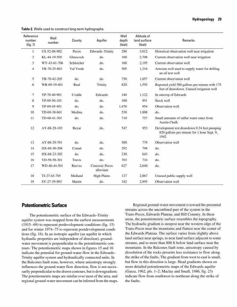
Hydrogeology 29
Table 2. Wells used to construct long-term hydrographs.
Reference number (fig. 7)
Well number County Aquifer
Well depth (feet)
Altitude of land surface
(feet)Remarks
1 US-52-08-902 Pecos Edwards–Trinity 290 3,012 Historical observation well near irrigation
2 KL-44-19-505 Glasscock do. 160 2,708 Current observation well near irrigation
3 WY-43-61-706 Schleicher do. 160 2,195 Current observation well
4 YR-70-25-603 Val Verde do. 505 1,216 Artesian well used to supply water for drilling an oil test well
5 YR-70-42-205 do. do. 750 1,057 Current observation well
6 WR-69-19-401 Real Trinity 820 1,595 Reported yield 500 gallons per minute with 175 feet of drawdown. Unused irrigation well
7 YP-70-40-901 Uvalde Edwards 140 1,122 In outcrop of Edwards
8 YP-69-50-101 do. do. 100 951 Stock well
9 YP-69-45-401 do. do. 1,476 954 Observation well
10 TD-69-38-601 Medina do. 538 1,008 do.
11 TD-68-41-301 do. do. 710 757 Small amounts of sulfur water enter from Austin Chalk
12 AY-68-29-103 Bexar do. 547 953 Development test drawdown 9.24 feet pumping 820 gallons per minute for 1 hour Sept. 9, 1942
13 AY-68-29-701 do. do. 500 779 Observation well
14 DX-68-30-208 Comal do. 292 798 do.
15 DX-68-23-302 do. do. 230 643 do.
16 YD-58-58-301 Travis do. 703 734 do.
17 WD-46-44-501 Reeves Cenozoic Pecos alluvium
627 2,640 do.
18 TJ-27-63-705 Midland High Plains 127 2,867 Unused public supply well
19 SY-27-39-903 Martin do. 182 2,895 Observation well
Potentiometric Surface
The potentiometric surface of the Edwards–Trinity aquifer system was mapped from the earliest measurements (1915–69) to represent predevelopment conditions (fig. 15) and for winter 1974–75 to represent postdevelopment condi-tions (fig. 16). In an isotropic aquifer (an aquifer in which hydraulic properties are independent of direction), ground-water movement is perpendicular to the potentiometric con-tours. The potentiometric maps shown in figures 15 and 16 indicate the potential for ground-water flow in the Edwards–Trinity aquifer system and hydraulically connected units. In the Balcones fault zone, however, where anisotropy strongly influences the ground-water flow direction, flow is not neces-sarily perpendicular to the drawn contours, but is downgradient. The potentiometric maps are similar over most of the area, and regional ground-water movement can be inferred from the maps.
Regional ground-water movement is toward the perennial streams across the unconfined part of the system in the Trans-Pecos, Edwards Plateau, and Hill Country. In these areas, the potentiometric surface resembles the topography. The hydraulic gradient is steepest near the western edge of the Trans-Pecos near the mountains and flattest near the center of the Edwards Plateau. The surface varies from slightly above land surface near springs, to near land surface adjacent to some streams, and to more than 800 ft below land surface near the mountains. In the Balcones fault zone, anisotropy caused by dissolution of the rocks presents less resistance to flow along the strike of the faults. The gradient from west to east is small, but flow in this direction is large. Head gradients shown on more detailed potentiometric maps of the Edwards aquifer (Garza, 1962, pls. 1–2; Maclay and Small, 1986, fig. 23)indicate flow from southwest to northeast along the strike of the faults.
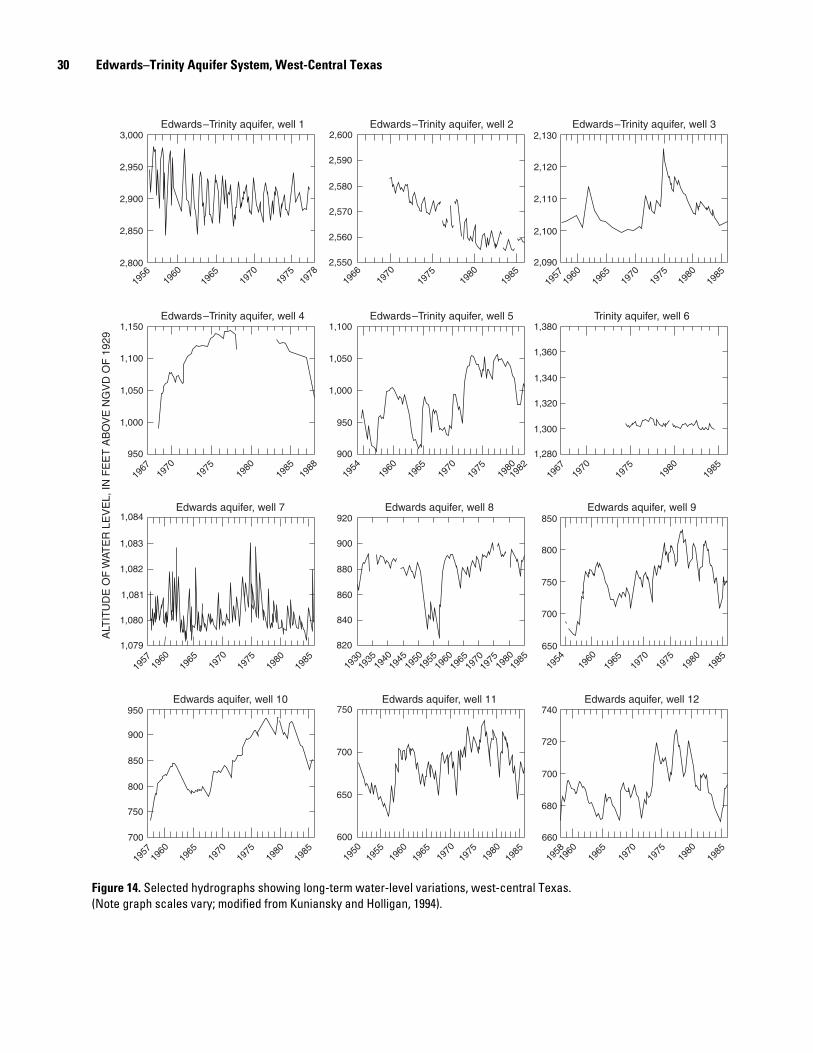
30 Edwards–Trinity Aquifer System, West-Central Texas
Figure 14. Selected hydrographs showing long-term water-level variations, west-central Texas. (Note graph scales vary; modified from Kuniansky and Holligan, 1994).
3,000
2,950
2,900
2,850
2,800
1,150
1,100
1,050
1,000
950
1,084
1,083
1,082
1,081
1,080
1,079
950
900
850
800
750
700
2,600
2,590
2,580
2,570
2,560
2,550
1,100
1,050
1,000
950
900
920
900
880
860
840
820
750
700
650
600
2,130
2,120
2,110
2,100
2,090
1,380
1,360
1,340
1,320
1,300
1,280
850
800
750
700
650
740
720
700
680
660
1956
1960
1965
1970
1975
1978
1957
1960
1965
1970
1975
1980
1985
1966
1970
1975
1980
1985
1967
1970
1975
1980
1985
1988
1954
1960
1965
1970
1975
198019
8219
6719
7019
7519
8019
85
1957
1960
1965
1970
1975
1980
1985
1930
1935
1940
1945
1950
1955
1960
1965
1970
1975
1980
1985
1954
1960
1965
1970
1975
1980
1985
1957
1960
1965
1970
1975
1980
1985
1950
1955
1960
1965
1970
1975
1980
1985
1958
1960
1965
1970
1975
1980
1985
Edwards–Trinity aquifer, well 1 Edwards–Trinity aquifer, well 2 Edwards–Trinity aquifer, well 3
Edwards–Trinity aquifer, well 4 Edwards–Trinity aquifer, well 5 Trinity aquifer, well 6
Edwards aquifer, well 7
Edwards aquifer, well 10
Edwards aquifer, well 8
Edwards aquifer, well 11
Edwards aquifer, well 9
Edwards aquifer, well 12
ALT
ITU
DE
OF
WAT
ER
LE
VE
L, IN
FE
ET
AB
OV
E N
GV
D O
F 1
929
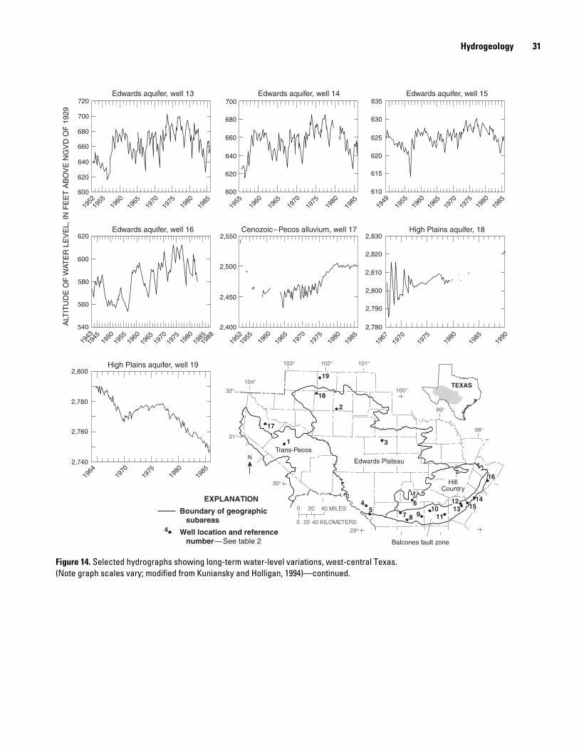
Hydrogeology 31
Figure 14. Selected hydrographs showing long-term water-level variations, west-central Texas. (Note graph scales vary; modified from Kuniansky and Holligan, 1994)—continued.
Well location and reference number—See table 2
Boundary of geographic subareas
EXPLANATION0 20 40 MILES
0 20 40 KILOMETERS
N
720
700
680
660
640
620
600
540
560
580
600
620
700
680
660
640
620
600
2,400
2,450
2,500
2,550
2,740
2,760
2,780
2,800
2,780
2,790
2,800
2,810
2,820
2,830
610
615
620
625
630
635
1952
1955
1960
1965
1970
1975
1980
1985
1955
1960
1965
1970
1975
1980
1985
1949
1955
1960
1965
1970
1975
1980
1985
194319
4519
5019
5519
6019
6519
7019
7519
8019
8519
8819
5219
5519
6019
6519
7019
7519
8019
8519
7019
7519
8019
8519
9019
67
1964
1970
1975
1980
1985
Edwards aquifer, well 13
Edwards aquifer, well 16
Edwards aquifer, well 14
Cenozoic–Pecos alluvium, well 17
Edwards aquifer, well 15
High Plains aquifer, 18
High Plains aquifer, well 19
ALT
ITU
DE
OF
WAT
ER
LE
VE
L, IN
FE
ET
AB
OV
E N
GV
D O
F 1
929
32°
31°
104°
102°103° 101°
100°
98°
99°
30°
29°
Trans-Pecos
Balcones fault zone
Edwards Plateau
HillCountry
19
18
2
17
1 3
4
4
57 8 9
1011
13
16
6 1215
14
TEXAS
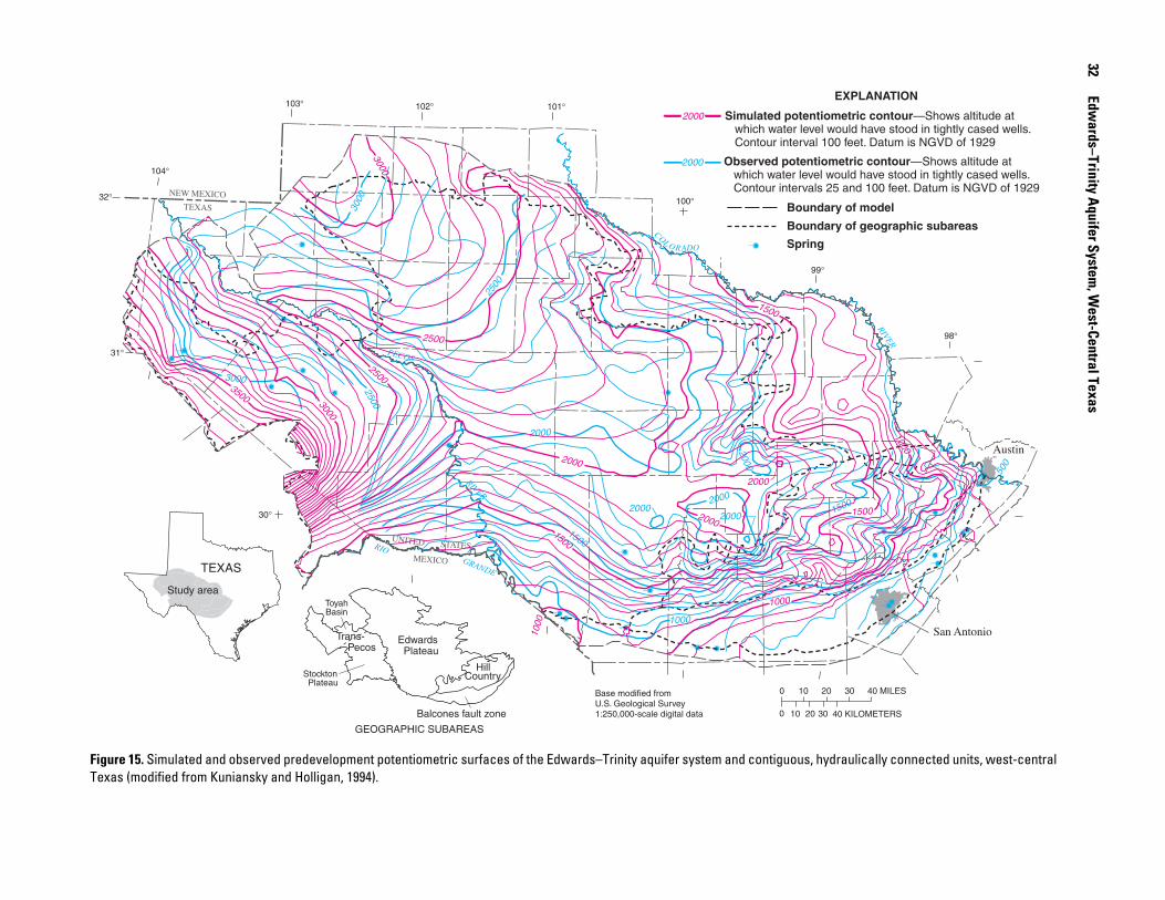
32 Edw
ards–Trinity Aquifer System
, West-Central Texas
Figure 15. Simulated and observed predevelopment potentiometric surfaces of the Edwards–Trinity aquifer system and contiguous, hydraulically connected units, west-central Texas (modified from Kuniansky and Holligan, 1994).
98°
99°
101°102°103°
104°
32°
31°
30°
NEW MEXICO
TEXAS
UNITED
MEXICO
STATES
GRANDE
RIO
San Antonio
Austin
PECOS
RIVER
COL ORADO
RIVER
0 10 20 30 40 MILES
0 10 20 30 40 KILOMETERS
Base modified from U.S. Geological Survey1:250,000-scale digital data
Spring
Boundary of model
Boundary of geographic subareas
Simulated potentiometric contour—Shows altitude at which water level would have stood in tightly cased wells. Contour interval 100 feet. Datum is NGVD of 1929
Observed potentiometric contour—Shows altitude at which water level would have stood in tightly cased wells. Contour intervals 25 and 100 feet. Datum is NGVD of 1929
2000
2000
EXPLANATION
100°
3000
3000
2500
2000
20002000
1500
1000
1500
2500
2000
2000
500
3000
1500
1500
2000
20001500
1000
1000
1000
2000
3000
3500
2500
2500
TEXAS
Study area
Edwards Plateau
Trans- Pecos
Hill Country
Balcones fault zone
GEOGRAPHIC SUBAREAS
ToyahBasin
Stockton Plateau
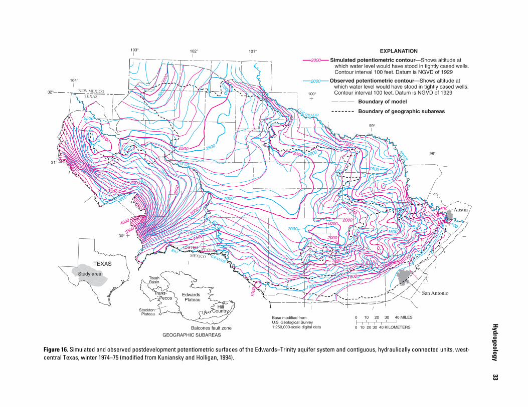
Hydrogeology
33
Figure 16. Simulated and observed postdevelopment potentiometric surfaces of the Edwards–Trinity aquifer system and contiguous, hydraulically connected units, west-central Texas, winter 1974–75 (modified from Kuniansky and Holligan, 1994).
NEW MEXICOTEXAS
UNITED
MEXICO
STATESGRANDE
RIO
San Antonio
Austin
PECOS
RIVERCOL ORADO
RIVER
98°
101°102°103°
99°
100°
104°
32°
31°
30°
0 10 20 30 40 MILES
0 10 20 30 40 KILOMETERS
Base modified from U.S. Geological Survey1:250,000-scale digital data
Boundary of model
Boundary of geographic subareas
Simulated potentiometric contour—Shows altitude at which water level would have stood in tightly cased wells. Contour interval 100 feet. Datum is NGVD of 1929
Observed potentiometric contour—Shows altitude at which water level would have stood in tightly cased wells. Contour interval 100 feet. Datum is NGVD of 1929
2000
2000
EXPLANATION
1500
3000
2500
2500
2500
25003000
3500 2000
15002000
1000
2000
1500
500
3000
2500
3500
2500
3000
4000
2500
2000
3500
1500
1000
2000
1500
1000
500
20002000
1500
2000
TEXAS
Study area
Edwards Plateau
Trans- Pecos
Hill Country
Balcones fault zone
GEOGRAPHIC SUBAREAS
ToyahBasin
Stockton Plateau
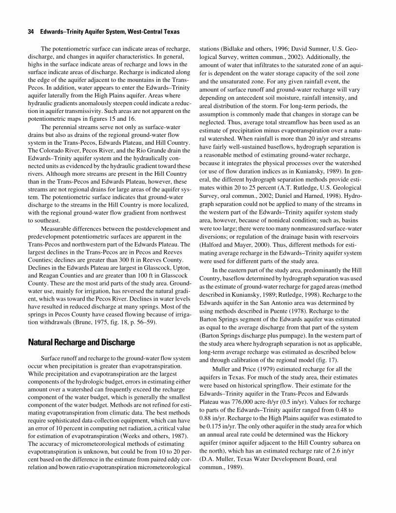
34 Edwards–Trinity Aquifer System, West-Central Texas
The potentiometric surface can indicate areas of recharge, discharge, and changes in aquifer characteristics. In general, highs in the surface indicate areas of recharge and lows in the surface indicate areas of discharge. Recharge is indicated along the edge of the aquifer adjacent to the mountains in the Trans-Pecos. In addition, water appears to enter the Edwards–Trinity aquifer laterally from the High Plains aquifer. Areas where hydraulic gradients anomalously steepen could indicate a reduc-tion in aquifer transmissivity. Such areas are not apparent on the potentiometric maps in figures 15 and 16.
The perennial streams serve not only as surface-water drains but also as drains of the regional ground-water flow system in the Trans-Pecos, Edwards Plateau, and Hill Country. The Colorado River, Pecos River, and the Rio Grande drain the Edwards–Trinity aquifer system and the hydraulically con-nected units as evidenced by the hydraulic gradient toward these rivers. Although more streams are present in the Hill Country than in the Trans-Pecos and Edwards Plateau, however, these streams are not regional drains for large areas of the aquifer sys-tem. The potentiometric surface indicates that ground-water discharge to the streams in the Hill Country is more localized, with the regional ground-water flow gradient from northwest to southeast.
Measurable differences between the postdevelopment and predevelopment potentiometric surfaces are apparent in the Trans-Pecos and northwestern part of the Edwards Plateau. The largest declines in the Trans-Pecos are in Pecos and Reeves Counties; declines are greater than 300 ft in Reeves County. Declines in the Edwards Plateau are largest in Glasscock, Upton, and Reagan Counties and are greater than 100 ft in Glasscock County. These are the most arid parts of the study area. Ground-water use, mainly for irrigation, has reversed the natural gradi-ent, which was toward the Pecos River. Declines in water levels have resulted in reduced discharge at many springs. Most of the springs in Pecos County have ceased flowing because of irriga-tion withdrawals (Brune, 1975, fig. 18, p. 56–59).
Natural Recharge and Discharge
Surface runoff and recharge to the ground-water flow system occur when precipitation is greater than evapotranspiration. While precipitation and evapotranspiration are the largest components of the hydrologic budget, errors in estimating either amount over a watershed can frequently exceed the recharge component of the water budget, which is generally the smallest component of the water budget. Methods are not refined for esti-mating evapotranspiration from climatic data. The best methods require sophisticated data-collection equipment, which can have an error of 10 percent in computing net radiation, a critical value for estimation of evapotranspiration (Weeks and others, 1987). The accuracy of micrometeorological methods of estimating evapotranspiration is unknown, but could be from 10 to 20 per-cent based on the difference in the estimate from paired eddy cor-relation and bowen ratio evapotranspiration micrometeorological
stations (Bidlake and others, 1996; David Sumner, U.S. Geo-logical Survey, written commun., 2002). Additionally, the amount of water that infiltrates to the saturated zone of an aqui-fer is dependent on the water storage capacity of the soil zone and the unsaturated zone. For any given rainfall event, the amount of surface runoff and ground-water recharge will vary depending on antecedent soil moisture, rainfall intensity, and areal distribution of the storm. For long-term periods, the assumption is commonly made that changes in storage can be neglected. Thus, average total streamflow has been used as an estimate of precipitation minus evapotranspiration over a natu-ral watershed. When rainfall is more than 20 in/yr and streams have fairly well-sustained baseflows, hydrograph separation is a reasonable method of estimating ground-water recharge, because it integrates the physical processes over the watershed (or use of flow duration indices as in Kuniansky, 1989). In gen-eral, the different hydrograph separation methods provide esti-mates within 20 to 25 percent (A.T. Rutledge, U.S. Geological Survey, oral commun., 2002; Daniel and Harned, 1998). Hydro-graph separation could not be applied to many of the streams in the western part of the Edwards–Trinity aquifer system study area, however, because of nonideal condition; such as, basins were too large; there were too many nonmeasured surface-water diversions; or regulation of the drainage basin with reservoirs (Halford and Mayer, 2000). Thus, different methods for esti-mating average recharge in the Edwards–Trinity aquifer system were used for different parts of the study area.
In the eastern part of the study area, predominantly the Hill Country, baseflow determined by hydrograph separation was used as the estimate of ground-water recharge for gaged areas (method described in Kuniansky, 1989; Rutledge, 1998). Recharge to the Edwards aquifer in the San Antonio area was determined by using methods described in Puente (1978). Recharge to the Barton Springs segment of the Edwards aquifer was estimated as equal to the average discharge from that part of the system (Barton Springs discharge plus pumpage). In the western part of the study area where hydrograph separation is not as applicable, long-term average recharge was estimated as described below and through calibration of the regional model (fig. 17).
Muller and Price (1979) estimated recharge for all the aquifers in Texas. For much of the study area, their estimates were based on historical springflow. Their estimate for the Edwards–Trinity aquifer in the Trans-Pecos and Edwards Plateau was 776,000 acre-ft/yr (0.5 in/yr). Values for recharge to parts of the Edwards–Trinity aquifer ranged from 0.48 to 0.88 in/yr. Recharge to the High Plains aquifer was estimated to be 0.175 in/yr. The only other aquifer in the study area for which an annual areal rate could be determined was the Hickory aquifer (minor aquifer adjacent to the Hill Country subarea on the north), which has an estimated recharge rate of 2.6 in/yr (D.A. Muller, Texas Water Development Board, oral commun., 1989).
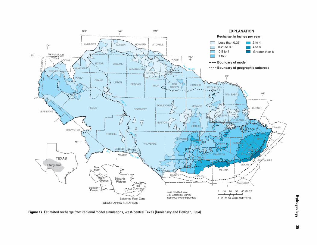
Hydrogeology
35
Figure 17. Estimated recharge from regional model simulations, west-central Texas (Kuniansky and Holligan, 1994).
ANDREWS MARTIN HOWARD
LOVING
WINKLER
ECTOR
REEVES
WARD
CU
LBE
RS
ON
STERLING
IRIONREAGAN
UPTON
GLASSCOCK
MIDLAND
PECOS
CRANE
JEFF DAVIS
BREWSTER
TERRELL
CROCKETT
NEW MEXICOTEXAS
UNITED
MEXICO
STATES
MITCHELL
COKE
MASON
TOMGREEN
CONCHOMCCULLOCH
SAN SABA
LLANO
BURNET
GILLESPIE BLANCOTRAVIS
KERR
BANDERA
KENDALL
HAYS
BEXAR
GUADALUPE
COMAL
ATASCOSA
MEDINA
EDWARDS
REAL
UVALDEKINNEY
VAL VERDE
SCHLEICHER MENARD
KIMBLE
SUTTON
GRANDE
RIO
PECOS
RIVERCOL ORADO
RIVER
101°102°103°
98°
99°
100°
104°
32°
31°
30°
TEXAS
Study area
Edwards Plateau
Trans- Pecos
Hill Country
Balcones Fault Zone
GEOGRAPHIC SUBAREAS
ToyahBasin
Stockton Plateau
Recharge, in inches per year
EXPLANATION
Less than 0.250.25 to 0.50.5 to 11 to 2
2 to 44 to 8
Greater than 8
Boundary of model
Boundary of geographic subareas
0 10 20 30 40 MILES
0 10 20 30 40 KILOMETERS
Base modified from U.S. Geological Survey1:250,000-scale digital data
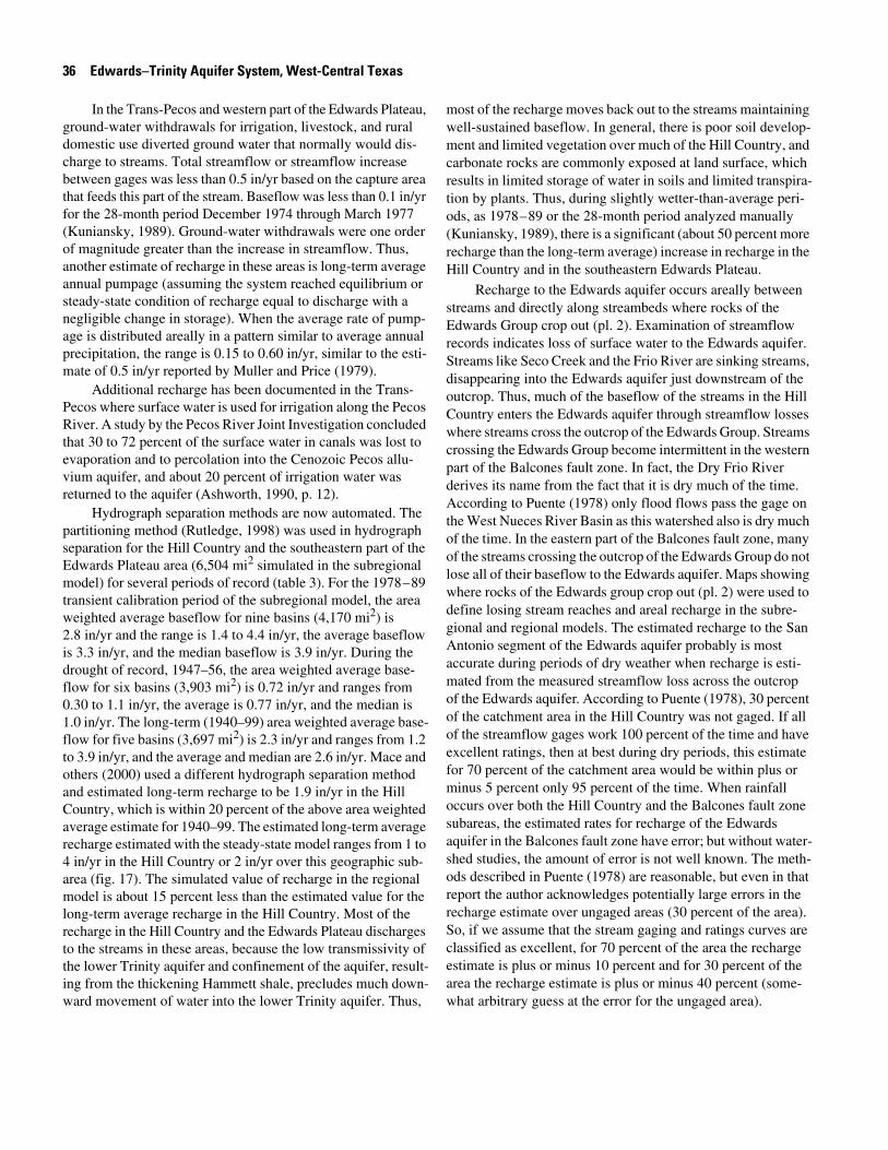
36 Edwards–Trinity Aquifer System, West-Central Texas
In the Trans-Pecos and western part of the Edwards Plateau, ground-water withdrawals for irrigation, livestock, and rural domestic use diverted ground water that normally would dis-charge to streams. Total streamflow or streamflow increase between gages was less than 0.5 in/yr based on the capture area that feeds this part of the stream. Baseflow was less than 0.1 in/yr for the 28-month period December 1974 through March 1977 (Kuniansky, 1989). Ground-water withdrawals were one order of magnitude greater than the increase in streamflow. Thus, another estimate of recharge in these areas is long-term average annual pumpage (assuming the system reached equilibrium or steady-state condition of recharge equal to discharge with a negligible change in storage). When the average rate of pump-age is distributed areally in a pattern similar to average annual precipitation, the range is 0.15 to 0.60 in/yr, similar to the esti-mate of 0.5 in/yr reported by Muller and Price (1979).
Additional recharge has been documented in the Trans-Pecos where surface water is used for irrigation along the Pecos River. A study by the Pecos River Joint Investigation concluded that 30 to 72 percent of the surface water in canals was lost to evaporation and to percolation into the Cenozoic Pecos allu-vium aquifer, and about 20 percent of irrigation water was returned to the aquifer (Ashworth, 1990, p. 12).
Hydrograph separation methods are now automated. The partitioning method (Rutledge, 1998) was used in hydrograph separation for the Hill Country and the southeastern part of the Edwards Plateau area (6,504 mi2 simulated in the subregional model) for several periods of record (table 3). For the 1978–89 transient calibration period of the subregional model, the area weighted average baseflow for nine basins (4,170 mi2) is 2.8 in/yr and the range is 1.4 to 4.4 in/yr, the average baseflow is 3.3 in/yr, and the median baseflow is 3.9 in/yr. During the drought of record, 1947–56, the area weighted average base-flow for six basins (3,903 mi2) is 0.72 in/yr and ranges from 0.30 to 1.1 in/yr, the average is 0.77 in/yr, and the median is 1.0 in/yr. The long-term (1940–99) area weighted average base-flow for five basins (3,697 mi2) is 2.3 in/yr and ranges from 1.2 to 3.9 in/yr, and the average and median are 2.6 in/yr. Mace and others (2000) used a different hydrograph separation method and estimated long-term recharge to be 1.9 in/yr in the Hill Country, which is within 20 percent of the above area weighted average estimate for 1940–99. The estimated long-term average recharge estimated with the steady-state model ranges from 1 to 4 in/yr in the Hill Country or 2 in/yr over this geographic sub-area (fig. 17). The simulated value of recharge in the regional model is about 15 percent less than the estimated value for the long-term average recharge in the Hill Country. Most of the recharge in the Hill Country and the Edwards Plateau discharges to the streams in these areas, because the low transmissivity of the lower Trinity aquifer and confinement of the aquifer, result-ing from the thickening Hammett shale, precludes much down-ward movement of water into the lower Trinity aquifer. Thus,
most of the recharge moves back out to the streams maintaining well-sustained baseflow. In general, there is poor soil develop-ment and limited vegetation over much of the Hill Country, and carbonate rocks are commonly exposed at land surface, which results in limited storage of water in soils and limited transpira-tion by plants. Thus, during slightly wetter-than-average peri-ods, as 1978–89 or the 28-month period analyzed manually (Kuniansky, 1989), there is a significant (about 50 percent more recharge than the long-term average) increase in recharge in the Hill Country and in the southeastern Edwards Plateau.
Recharge to the Edwards aquifer occurs areally between streams and directly along streambeds where rocks of the Edwards Group crop out (pl. 2). Examination of streamflow records indicates loss of surface water to the Edwards aquifer. Streams like Seco Creek and the Frio River are sinking streams, disappearing into the Edwards aquifer just downstream of the outcrop. Thus, much of the baseflow of the streams in the Hill Country enters the Edwards aquifer through streamflow losses where streams cross the outcrop of the Edwards Group. Streams crossing the Edwards Group become intermittent in the western part of the Balcones fault zone. In fact, the Dry Frio River derives its name from the fact that it is dry much of the time. According to Puente (1978) only flood flows pass the gage on the West Nueces River Basin as this watershed also is dry much of the time. In the eastern part of the Balcones fault zone, many of the streams crossing the outcrop of the Edwards Group do not lose all of their baseflow to the Edwards aquifer. Maps showing where rocks of the Edwards group crop out (pl. 2) were used to define losing stream reaches and areal recharge in the subre-gional and regional models. The estimated recharge to the San Antonio segment of the Edwards aquifer probably is most accurate during periods of dry weather when recharge is esti-mated from the measured streamflow loss across the outcrop of the Edwards aquifer. According to Puente (1978), 30 percent of the catchment area in the Hill Country was not gaged. If all of the streamflow gages work 100 percent of the time and have excellent ratings, then at best during dry periods, this estimate for 70 percent of the catchment area would be within plus or minus 5 percent only 95 percent of the time. When rainfall occurs over both the Hill Country and the Balcones fault zone subareas, the estimated rates for recharge of the Edwards aquifer in the Balcones fault zone have error; but without water-shed studies, the amount of error is not well known. The meth-ods described in Puente (1978) are reasonable, but even in that report the author acknowledges potentially large errors in the recharge estimate over ungaged areas (30 percent of the area). So, if we assume that the stream gaging and ratings curves are classified as excellent, for 70 percent of the area the recharge estimate is plus or minus 10 percent and for 30 percent of the area the recharge estimate is plus or minus 40 percent (some-what arbitrary guess at the error for the ungaged area).
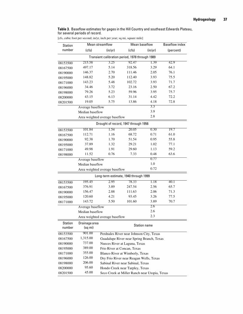
Hydrogeology 37
Table 3. Baseflow estimates for gages in the Hill Country and southeast Edwards Plateau, for several periods of record.[cfs, cubic foot per second; in/yr, inch per year; sq mi, square mile]
Station number
Mean streamflow Mean baseflow Baseflow index
(cfs) (in/yr) (cfs) (in/yr) (percent)
Transient calibration period, 1978 through 1989
08153500 215.58 3.25 92.47 1.39 42.9
08167500 497.17 5.14 318.56 3.29 64.1
08190000 146.37 2.70 111.46 2.05 76.1
08195000 148.82 5.20 112.40 3.93 75.5
08171000 143.23 5.48 102.72 3.93 71.7
08196000 34.46 3.72 23.16 2.50 67.2
08198000 79.26 5.23 59.96 3.95 75.7
08200000 43.15 6.13 31.14 4.42 72.2
08201500 19.05 5.75 13.86 4.18 72.8
Average baseflow 3.3
Median baseflow 3.9
Area weighted average baseflow 2.8
Drought of record, 1947 through 1956
08153500 101.84 1.54 20.05 0.30 19.7
08167500 112.71 1.16 68.72 0.71 61.0
08190000 92.38 1.70 51.54 0.95 55.8
08195000 37.89 1.32 29.21 1.02 77.1
08171000 49.98 1.91 29.60 1.13 59.2
08198000 11.52 0.76 7.33 0.48 63.6
Average baseflow 0.77
Median baseflow 1.0
Area weighted average baseflow 0.72
Long-term estimate, 1940 through 1999
08153500 195.45 2.95 78.33 1.18 40.1
08167500 376.91 3.89 247.54 2.56 65.7
08190000 156.47 2.88 111.63 2.06 71.3
08195000 120.60 4.21 93.45 3.26 77.5
08171000 143.72 5.50 101.60 3.89 70.7
Average baseflow 2.6
Median baseflow 2.6
Area weighted average baseflow 2.3
Station number
Drainage area (sq mi) Station name
08153500 901.00 Perdnales River near Johnson City, Texas08167500 1,315.00 Guadalupe River near Spring Branch, Texas08190000 737.00 Nueces River at Laguna, Texas08195000 389.00 Frio River at Concan, Texas08171000 355.00 Blanco River at Wimberly, Texas08196000 126.00 Dry Frio River near Reagan Wells, Texas08198000 206.00 Sabinal River near Sabinal, Texas08200000 95.60 Hondo Creek near Tarpley, Texas08201500 45.00 Seco Creek at Miller Ranch near Utopia, Texas
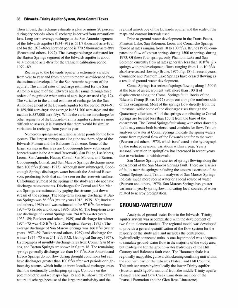
38 Edwards–Trinity Aquifer System, West-Central Texas
Then at best, the recharge estimate is plus or minus 20 percent during dry periods when all recharge is derived from streamflow loss. Long-term average recharge to the San Antonio segment of the Edwards aquifer (1934–91) is 651.7 thousand acre-ft/yr and for the 1978–89 calibration period is 770.5 thousand acre-ft/yr (Brown and others, 1992). The average recharge estimated for the Barton Springs segment of the Edwards aquifer is about 41.4 thousand acre-ft/yr for the transient calibration period 1979–89.
Recharge to the Edwards aquifer is extremely variable from year to year and from month to month as evidenced from the estimate developed for the San Antonio segment of the aquifer. The annual rates of recharge estimated for the San Antonio segment of the Edwards aquifer range through three orders of magnitude when units of acre-ft/yr are used (fig. 12). The variance in the annual estimate of recharge for the San Antonio segment of the Edwards aquifer for the period 1934–91 is 189,500 acre-ft/yr, the average is 651,700 acre-ft/yr, and the median is 557,000 acre-ft/yr. While the variance in recharge for other segments of the Edwards–Trinity aquifer system are more difficult to assess, it is assumed that there would be similar variations in recharge from year to year.
Numerous springs are natural discharge points for the flow system. The largest springs are along the southern edge of the Edwards Plateau and the Balcones fault zone. Some of the larger springs in this area are Goodenough (now submerged beneath water in the Amistad Reservoir), San Felipe, Las Moras, Leona, San Antonio, Hueco, Comal, San Marcos, and Barton. Goodenough, Comal, and San Marcos Springs discharge more than 100 ft3/s (Brune, 1975). Although now submerged, Good-enough Springs discharges water beneath the Amistad Reser-voir, producing boils that can be seen on the reservoir surface. Unfortunately, most of the springs in the study area do not have discharge measurements. Discharges for Comal and San Mar-cos Springs are estimated by gaging the streams just down-stream of the springs. The long-term average discharge at Bar-ton Springs was 56 ft3/s (water years 1918, 1979–89; Buckner and others, 1989) and was estimated to be 97 ft3/s for winter 1974–75 (Slade and others, 1986, table 6). The long-term aver-age discharge of Comal Springs was 294 ft3/s (water years 1933–89; Buckner and others, 1989) and discharge for winter 1974–75 was 415 ft3/s (U.S. Geological Survey, 1975). The average discharge of San Marcos Springs was 166 ft3/s (water years 1957–89; Buckner and others, 1989) and discharge for winter 1974–75 was 241 ft3/s (U.S. Geological Survey, 1975). Hydrographs of monthly discharge rates from Comal, San Mar-cos, and Barton Springs are shown in figure 18. The remaining springs generally discharge less than 100 ft3/s. San Antonio and Hueco Springs do not flow during drought conditions but can have discharges greater than 100 ft3/s after wet periods or high-intensity storms, which indicate more localized recharge areas than the continually discharging springs. Contours on the potentiometric surface maps (figs. 15 and 16) show little of this natural discharge because of the large transmissivity and the
regional anisotropy of the Edwards aquifer and the scale of the maps and contour intervals used.
Prior to ground-water development in the Trans-Pecos, Phantom Lake, San Solomon, Leon, and Comanche Springs flowed at rates ranging from 10 to 100 ft3/s. Brune (1975) com-pares the flow of known springs during 1500 to springs during 1973. Of these four springs, only Phantom Lake and San Solomon currently flow at rates generally less than 10 ft3/s. Six springs with predevelopment flows ranging from 1 to 10 ft3/s also have ceased flowing (Brune, 1975, fig. 18). In recent years, Comanche and Phantom Lake Springs have ceased flowing as a result of ground-water development.
Comal Springs is a series of springs flowing along 4,500 ft at the base of an escarpment with more than 100 ft of displacement along the Comal Springs fault. Rocks of the Edwards Group (Rose, 1972) crops out along the northern side of this escarpment. Most of the springs flow directly from the limestone, while some of the discharge rises through the Quaternary alluvium. All of the springs contributing to Comal Springs are located less than 150 ft from the base of the escarpment. The Comal Springs fault along with other downdip faults may create both barriers to and conduits for flow. Tritium analyses of water at Comal Springs indicate the spring waters come from regional flow of the Edwards aquifer to the west (Pearson and others, 1975), which is reflected in the hydrograph by the reduced seasonal variations within a year. Yearly seasonal variation in springflow has increased in recent years due to variations in withdrawals.
San Marcos Springs is a series of springs flowing along the escarpment of the San Marcos Springs fault. There are a series of faults near the springs including the eastern extension of the Comal Springs fault. Tritium analyses of San Marcos Springs indicate much more recent water or a local source of water (Pearson and others, 1975). San Marcos Springs has greater variance in yearly springflow, indicating local sources of water related to nearby precipitation.
GROUND-WATER FLOW
Analysis of ground-water flow in the Edwards–Trinity aquifer system was accomplished with the development of two finite-element models. The regional model was developed to provide a general quantification of the flow system for the majority of the study area and includes the contiguous, hydraulically connected units. A one-layer model was adequate to simulate ground-water flow in the majority of the study area, but inadequate for the ground-water hydrology of the Hill Country and Balcones fault zone. The Hammett shale is a regionally mappable, gulfward thickening confining unit within the southern part of the Edwards Plateau and Hill Country. This unit separates hydraulically the lower Trinity aquifer (Hosston and Sligo Formations) from the middle Trinity aquifer (Hensel Sand and Cow Creek Limestone member of the Pearsall Formation and the Glen Rose Limestone).
Ground-Water Flow 39
Figure 18. Historical monthly springflow discharge at Comal, San Marcos, and Barton Springs, central Texas. See plate 2 for spring locations.
0
500
100
200
300
400
0
500
100
200
300
400
0
500
100
200
300
400
1910 20001920 1930 1940 1950 1960 1970 1980 1990
DIS
CH
AR
GE
, IN
CU
BIC
FE
ET
PE
R S
EC
ON
D
Comal Springs
San Marcos Springs
Barton Springs
In the southern part of the Balcones fault zone, the Navarro–Del Rio confining unit overlies the Edwards aquifer. Thus, a multi-layer model was developed for the subregion that includes the Hill Country and Balcones fault zone. The subre-gional model area extends into the southeastern part of the Edwards Plateau north and west of the Hill Country and Bal-cones fault zone where the aquifers form a shallow one-layer water-table system.
The regional model was calibrated to represent steady-state conditions, reflecting long-term conditions. This approach
may be adequate for the majority of the study area in the
Trans-Pecos, Edwards Plateau, and Hill Country, but is
inadequate for the Balcones fault zone where the relatively
dynamic Edwards aquifer receives direct recharge along
streams that cross the outcrop of the Edwards Group during
storm events. Long-term water-level hydrographs provide some
indication that steady-state conditions are rare in the Edwards
aquifer (fig. 14). Thus, the subregional model was
accomplished with transient simulation.
40 Edwards–Trinity Aquifer System, West-Central Texas
Regional Steady-State Simulations of Ground-Water Flow
Steady-state model simulations for the entire aquifer system (55,600 mi2, pl. 1) were accomplished using a two-dimensional one-layer model for ground-water flow (Kuniansky, 1990a). The steady-state simulations were for predevelopment conditions and winter 1974–75 conditions. The winter of 1974–75 (December 1974 through February 1975) was selected for simulation because (1) the system is nearest to steady-state conditions during winter; (2) less loss of ground water is lost to evaporation, irrigation withdrawals, and transpiration during winter; and (3) water use in parts of the study area had peaked by winter 1974–75. The details of the steady-state regional model calibration and sensitivity analysis are described in Kuniansky and Holligan (1994).
Regional Model Development
In developing a numerical model of an aquifer system, many simplifications are required in order to approximate the system. Flow through most porous media is three-dimensional, but most aquifers are several orders of magnitude thinner in the vertical dimension than in the horizontal dimension. In the case of the Edwards–Trinity aquifer system, the horizontal dimen-sion is more than four orders of magnitude greater than the ver-tical dimension. Therefore, flow can be approximated as two-dimensional and horizontal where the simulated water level is the vertically averaged water level within the aquifer. A gener-alized section showing the geologic units simulated as one layer is shown in figure 5. Another simplification for modeling was to assume steady-state conditions. For a large part of the study area, few data are available for transient simulation; and, in gen-eral, hydrographs for wells located away from principal ground-water withdrawal points do not indicate large seasonal fluctua-tions (fig. 14). Two hydrographs indicate mining of water; thus, steady-state conditions may not exist near wells 1, 2, and 19 (fig. 14). In the Balcones fault zone, the Edwards aquifer is rarely under steady-state conditions. Long-term water-level records show that annual fluctuations from 50 to 100 ft are com-mon (Nalley, 1989, table 5). During winter 1974–75, water lev-els were rising in the Balcones fault zone; and, thus, water was moving into storage within the aquifer during that time.
In a steady-state simulation, recharge must equal discharge and there can be no change in storage. In order to account for the amount of water that would go into storage during the winter of 1974–75, the amount of actual recharge to the Edwards aquifer could be greater than the amount simulated. The average water-level rise in 16 wells throughout the Edwards aquifer was 4.2 ft from December 1974 through February 1975. The average rise in four wells in Bexar County was 3.75 ft. Using the previously discussed water-level storage relation of Garza (1966), which indicates that about 40,000 acre-ft of water is taken into storage for each foot of water-level rise, the estimated amount of water that went into storage was 150,000 acre-ft for
the 3-month period. This amount is about one-half the estimated recharge for that period. Thus, the recharge applied in the steady-state simulation was reduced to one-half the estimated transient recharge of the 3-month period.
The ground-water flow equation solved by the flow model is the continuity equation for flow with incorporation of Darcy’s law, derived from the principal of conservation of mass and assumptions that water is incompressible and of constant visco-sity (Raudkivi and Callander, 1976, p. 43; Bouwer, 1978, p. 202; Bear, 1979, p. 93). This equation is valid for ground-water flow problems when the velocity of ground water is slow and lami-nar. In karstic terrains, it is quite possible for flow through cav-erns and solution channels to be turbulent. Thus, the equation is not valid for the entire flow domain of the Edwards–Trinity aquifer system. A simplification is to assume laminar flow everywhere and an effective transmissivity that is uniform throughout each element of the model such that conservation of mass is preserved along with known hydraulic gradients.
The finite-element method was chosen to simulate the ground-water hydrogeology of the Balcones fault zone, because the method allows for the direction of anisotropy to vary areally. This factor was the most important reason for choosing the finite-element method rather than the finite-difference method. While the general orientation of the en echelon faults in the Balcones fault zone is from southwest to northeast, locally faults are not parallel to the regional trend. Previous determin-istic models developed in the study area (Klemt and others, 1979; Slade and others, 1985; Maclay and Land, 1988, Thorkild-sen and McElhaney, 1992) used the finite-difference method. Maclay and Land (1988) examined the effects of anisotropy by orienting the finite-difference grid in the prevailing direction of the major faults in the San Antonio segment of the Edwards aquifer. Thorkildsen and McElhaney (1992) incorporated anisotropy and recalibrated the model developed by Klemt and others (1979) with monthly stress periods. The model study of the Austin area (Slade and others, 1985) did not simulate the effects of faults and joints by incorporating anisotropy.
Another advantage of using the finite-element method is the flexibility of developing an irregularly spaced mesh of tri-angular elements, which allows for variably spaced elements with smaller elements in areas of high topography (more local flow zones) and better incorporation of drainage features in these areas (better simulation of local discharge). These ele-ments represent parts of the aquifer system with similar hydrau-lic properties. Although the design of the finite-element mesh is tedious, the irregular external and internal boundaries of the flow system can be more accurately located. Stream-aquifer interaction is important across large areas of the aquifer system. When using the finite-element method, streams are simulated along element sides. The regional model has elements varying from about 1 mi2 increasing up to the largest, which is about 70 mi2 in the Edwards Plateau where the topography is relatively flat. In the Hill Country, finite-elements range from about 2 to 15 mi2, with most elements less than 5 mi2. Stream geometry is simplified but located more accurately than in earlier RASA studies, such as the Southeastern Coastal Plain RASA, which
Ground-Water Flow 41
had equal-spaced finite-difference grids of 64 mi2 (Barker and Pernik, 1994). The Southeastern Coastal Plain RASA study model could not simulate 80 percent of the recharge, while keeping transmissivity in an acceptable range because of the huge equally spaced finite-difference grid employed in the modeling effort (R.A. Barker, U.S. Geological Survey, oral commun., 1995).
Local ground-water flow entering and leaving a system within the same finite-difference cell cannot be simulated (Wil-liamson and others, 1989). By using the variably spaced finite-element mesh, the effect of model scale and discretization can be minimized but not completely eliminated. The scale issue is difficult to resolve because the exact quantities of local versus intermediate versus regional (deep recharge) flow in any model are uncertain. The uncertainty results from the fact that recharge and transmissivity are correlated in the ground-water flow equa-tion, which means that an error in recharge can be compensated for by an error in transmissivity. There are no methods to know beforehand how much of a reduction in recharge (equivalent to the amount of local ground-water flow that cannot simulated) is required given the model discretization. Generally, efforts are made to reduce recharge and keep the transmissivity values used in the simulation within the range of known transmissivity.
Finite-Element Method
Solution of the steady-state ground-water flow equation has been discussed in numerous textbooks, such as Remson and others (1971), Bathe and Wilson (1976), Zienkiewicz (1977), Wang and Anderson (1982), Huyakorn and Pinder (1983), Reddy (1986), and Bear and Verruijt (1987). The finite-element method of solving the flow equation differs from the finite-dif-ference method in that it involves piece-wise approximation of the flow domain. The flow domain is broken into discrete sub-domains, called finite elements. The simplest element is a trian-gular element with linear sides. The computer program devel-oped for regional simulations uses three-nodal triangular finite elements. The computer program incorporates three types of boundary conditions: constant head, constant flux, and head-dependent flux which is documented in Kuniansky (1990a).
Regional Finite-Element Mesh and Lateral Boundaries
The finite-element mesh designed for the regional model is shown on plate 1. Because the Edwards–Trinity aquifer system is unconfined across most of the model area, the mesh was designed on the basis of surface-water drainage divides and streams across the Trans-Pecos, Edwards Plateau, and Hill Country. In the Balcones fault zone, the mesh was designed with elements aligned along the transmissivity subregions defined by Maclay and Small (1986, fig. 20) and along the Haby Crossing and Pearson faults (fig. 2). The mesh was designed such that element sides approximated the boundaries of the geo-graphic subareas shown in figure 1.
The lateral boundaries of the model were defined along hydrologic boundaries where possible. The northeastern bound-ary of the model follows the Colorado River. The southwestern
boundary follows the Rio Grande. These two rivers are simu-lated as head-dependent sinks. The southeastern boundary is simulated as a no-flow boundary, placed parallel with and downdip of the freshwater/saline-water transition zone. The updip limit of the transition zone (1,000-milligrams per liter line of equal dissolved solids concentration) also marks a sharp change in aquifer transmissivity from more than 100,000 ft2/d on the freshwater side of the transition zone to less than 1,000 ft2/d on the brackish-water side. The western boundary in the Trans-Pecos follows the edge of the Cretaceous rocks along the eastern edge of the mountain ranges. This boundary is simulated by head-dependent source nodes. Water enters the Edwards–Trinity aquifer system at the western edge of the Trans-Pecos from rainfall, which percolates into the alluvial fans at the base of the mountains and then into the regional aquifer. A no-flow boundary is placed within the Cenozoic Pecos alluvium aquifer where a Paleozoic ridge of low permeability rocks results in lit-tle or no saturated thickness of the aquifer. The only lateral boundary of the model, which is somewhat arbitrary, is the head-dependent source or sink boundary placed within the High Plains aquifer. The boundary types are indicated on plate 1.
Internal Boundaries
Perennial streams form the majority of the internal bound-aries of the model, the most important of which is the Pecos River. Since the river has incised into the Edwards–Trinity aquifer, forming a regional drain, it is simulated as a head-dependent source or sink. All other perennial streams inside the model area are simulated in a similar manner. The perennial streams were identified on 7.5-minute U.S. Geological Survey topographic maps, and stream stage elevations were estimated by interpolating streambed altitudes along reaches between topographic contours crossing the streams. The dashed lines along the upstream reaches of the Concho River and Beals Creek (pl. 1) represent segments of the two streams that were simulated in the predevelopment simulation but not in the win-ter 1974–75 simulation. After development, ground-water lev-els dropped below these streambeds and the reaches became inactive as drains of the ground-water system.
In the Balcones fault zone, the Pearson and Haby Crossing faults create internal boundaries. Each has displaced 100 percent of the Edwards aquifer (fig. 2). The displacement horizontally juxtaposes confining units and less permeable aquifer units with the Edwards aquifer (fig. 5, pl. 1). In the finite-element model, elements are aligned along these two faults, and a complete discontinuity in the model layer is simulated along parts of these faults. These two lines of discontinuity are shown on plate 1.
Water Budgets from Steady-State Regional Simulations
In a simplified model of the aquifer system, such as the two-dimensional finite-element model described in this report, water enters (recharges) or exits (discharges) the aquifer at nodes and moves horizontally. Because steady-state conditions are imposed, recharge equals discharge in each simulation. The
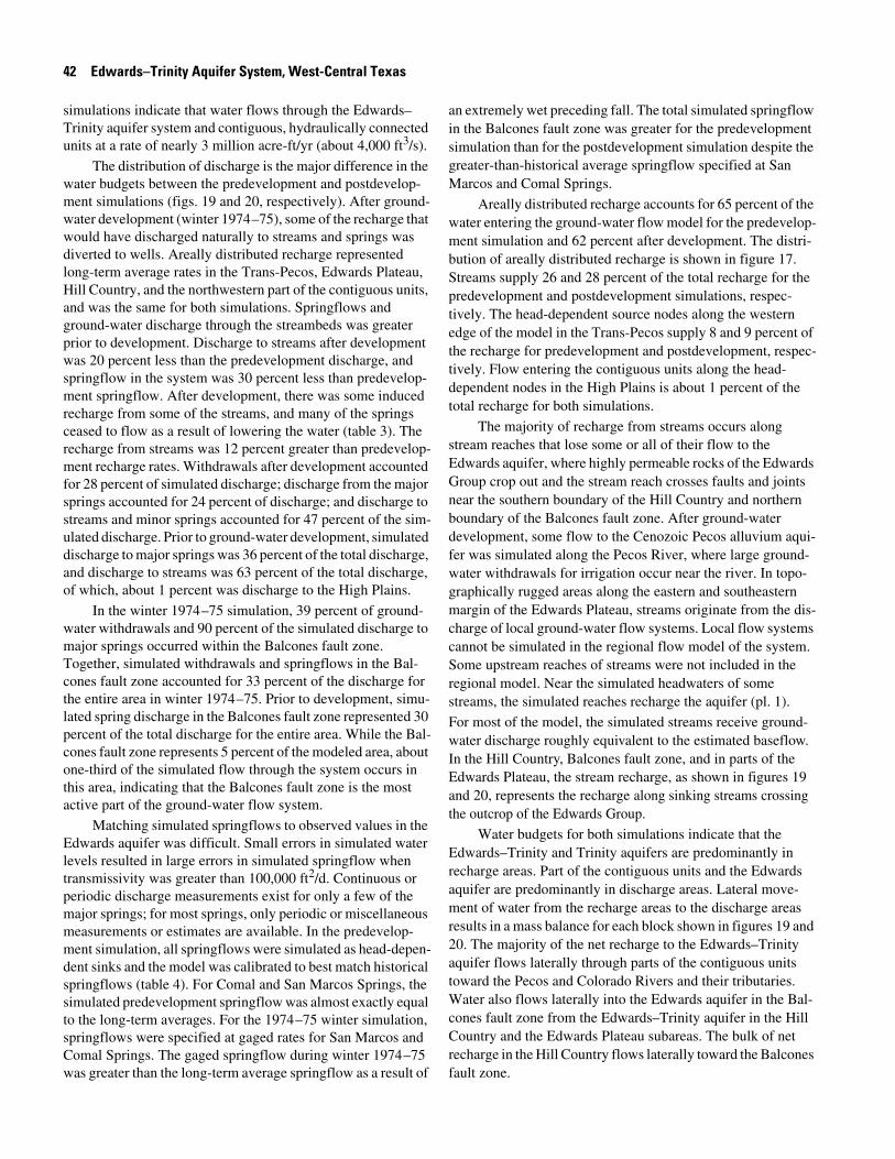
42 Edwards–Trinity Aquifer System, West-Central Texas
simulations indicate that water flows through the Edwards–Trinity aquifer system and contiguous, hydraulically connected units at a rate of nearly 3 million acre-ft/yr (about 4,000 ft3/s).
The distribution of discharge is the major difference in the water budgets between the predevelopment and postdevelop-ment simulations (figs. 19 and 20, respectively). After ground-water development (winter 1974–75), some of the recharge that would have discharged naturally to streams and springs was diverted to wells. Areally distributed recharge represented long-term average rates in the Trans-Pecos, Edwards Plateau, Hill Country, and the northwestern part of the contiguous units, and was the same for both simulations. Springflows and ground-water discharge through the streambeds was greater prior to development. Discharge to streams after development was 20 percent less than the predevelopment discharge, and springflow in the system was 30 percent less than predevelop-ment springflow. After development, there was some induced recharge from some of the streams, and many of the springs ceased to flow as a result of lowering the water (table 3). The recharge from streams was 12 percent greater than predevelop-ment recharge rates. Withdrawals after development accounted for 28 percent of simulated discharge; discharge from the major springs accounted for 24 percent of discharge; and discharge to streams and minor springs accounted for 47 percent of the sim-ulated discharge. Prior to ground-water development, simulated discharge to major springs was 36 percent of the total discharge, and discharge to streams was 63 percent of the total discharge, of which, about 1 percent was discharge to the High Plains.
In the winter 1974–75 simulation, 39 percent of ground-water withdrawals and 90 percent of the simulated discharge to major springs occurred within the Balcones fault zone. Together, simulated withdrawals and springflows in the Bal-cones fault zone accounted for 33 percent of the discharge for the entire area in winter 1974–75. Prior to development, simu-lated spring discharge in the Balcones fault zone represented 30 percent of the total discharge for the entire area. While the Bal-cones fault zone represents 5 percent of the modeled area, about one-third of the simulated flow through the system occurs in this area, indicating that the Balcones fault zone is the most active part of the ground-water flow system.
Matching simulated springflows to observed values in the Edwards aquifer was difficult. Small errors in simulated water levels resulted in large errors in simulated springflow when transmissivity was greater than 100,000 ft2/d. Continuous or periodic discharge measurements exist for only a few of the major springs; for most springs, only periodic or miscellaneous measurements or estimates are available. In the predevelop-ment simulation, all springflows were simulated as head-depen-dent sinks and the model was calibrated to best match historical springflows (table 4). For Comal and San Marcos Springs, the simulated predevelopment springflow was almost exactly equal to the long-term averages. For the 1974–75 winter simulation, springflows were specified at gaged rates for San Marcos and Comal Springs. The gaged springflow during winter 1974–75 was greater than the long-term average springflow as a result of
an extremely wet preceding fall. The total simulated springflow in the Balcones fault zone was greater for the predevelopment simulation than for the postdevelopment simulation despite the greater-than-historical average springflow specified at San Marcos and Comal Springs.
Areally distributed recharge accounts for 65 percent of the water entering the ground-water flow model for the predevelop-ment simulation and 62 percent after development. The distri-bution of areally distributed recharge is shown in figure 17. Streams supply 26 and 28 percent of the total recharge for the predevelopment and postdevelopment simulations, respec-tively. The head-dependent source nodes along the western edge of the model in the Trans-Pecos supply 8 and 9 percent of the recharge for predevelopment and postdevelopment, respec-tively. Flow entering the contiguous units along the head-dependent nodes in the High Plains is about 1 percent of the total recharge for both simulations.
The majority of recharge from streams occurs along stream reaches that lose some or all of their flow to the Edwards aquifer, where highly permeable rocks of the Edwards Group crop out and the stream reach crosses faults and joints near the southern boundary of the Hill Country and northern boundary of the Balcones fault zone. After ground-water development, some flow to the Cenozoic Pecos alluvium aqui-fer was simulated along the Pecos River, where large ground-water withdrawals for irrigation occur near the river. In topo-graphically rugged areas along the eastern and southeastern margin of the Edwards Plateau, streams originate from the dis-charge of local ground-water flow systems. Local flow systems cannot be simulated in the regional flow model of the system. Some upstream reaches of streams were not included in the regional model. Near the simulated headwaters of some streams, the simulated reaches recharge the aquifer (pl. 1).
For most of the model, the simulated streams receive ground-water discharge roughly equivalent to the estimated baseflow. In the Hill Country, Balcones fault zone, and in parts of the Edwards Plateau, the stream recharge, as shown in figures 19 and 20, represents the recharge along sinking streams crossing the outcrop of the Edwards Group.
Water budgets for both simulations indicate that the Edwards–Trinity and Trinity aquifers are predominantly in recharge areas. Part of the contiguous units and the Edwards aquifer are predominantly in discharge areas. Lateral move-ment of water from the recharge areas to the discharge areas results in a mass balance for each block shown in figures 19 and 20. The majority of the net recharge to the Edwards–Trinity aquifer flows laterally through parts of the contiguous units toward the Pecos and Colorado Rivers and their tributaries. Water also flows laterally into the Edwards aquifer in the Bal-cones fault zone from the Edwards–Trinity aquifer in the Hill Country and the Edwards Plateau subareas. The bulk of net recharge in the Hill Country flows laterally toward the Balcones fault zone.
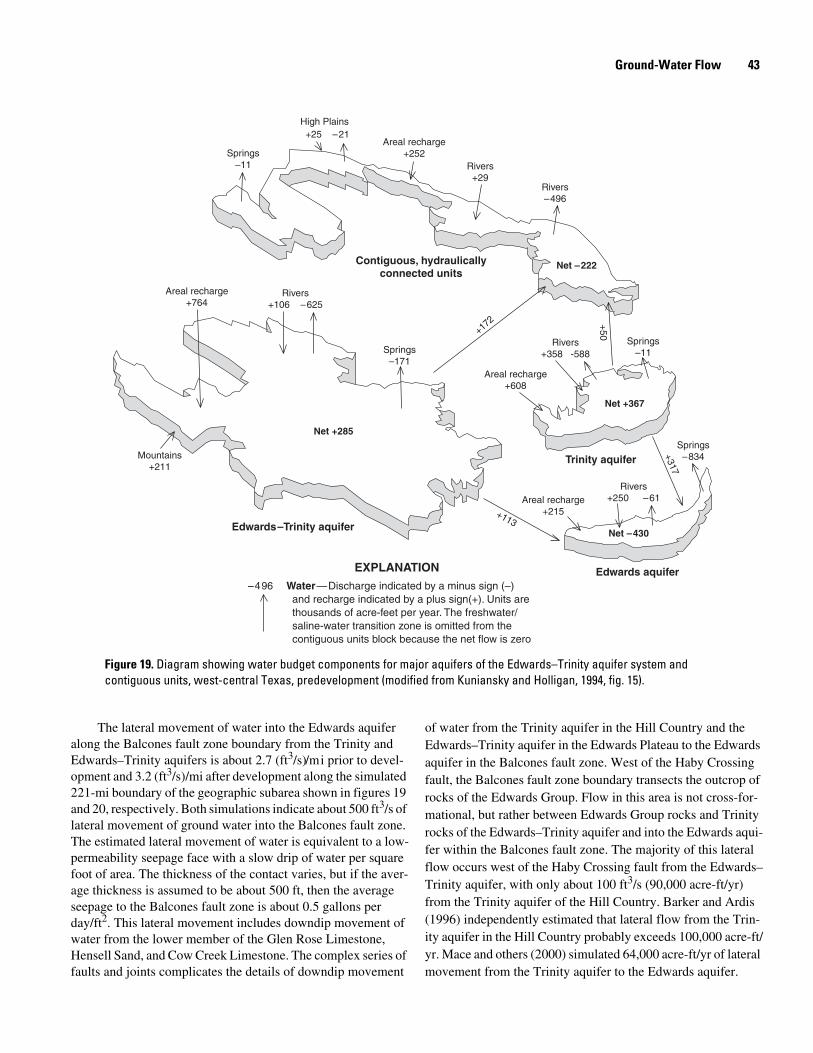
Ground-Water Flow 43
Figure 19. Diagram showing water budget components for major aquifers of the Edwards–Trinity aquifer system and contiguous units, west-central Texas, predevelopment (modified from Kuniansky and Holligan, 1994, fig. 15).
–496
Springs–11
+25 –21Areal recharge
+252Rivers
+29Rivers–496
Net –222
Areal recharge+764
Rivers+106 –625
Springs–171
+172
Mountains+211
Net +285
Areal recharge+608
Rivers+358 -588
Springs–11
+50
Net +367
Springs–834+317
Rivers+250 –61Areal recharge
+215+113Net –430
Contiguous, hydraulicallyconnected units
Edwards–Trinity aquifer
Trinity aquifer
Edwards aquiferWater—Discharge indicated by a minus sign (–) and recharge indicated by a plus sign(+). Units are thousands of acre-feet per year. The freshwater/ saline-water transition zone is omitted from the contiguous units block because the net flow is zero
EXPLANATION
High Plains
The lateral movement of water into the Edwards aquifer along the Balcones fault zone boundary from the Trinity and Edwards–Trinity aquifers is about 2.7 (ft3/s)/mi prior to devel-opment and 3.2 (ft3/s)/mi after development along the simulated 221-mi boundary of the geographic subarea shown in figures 19 and 20, respectively. Both simulations indicate about 500 ft3/s of lateral movement of ground water into the Balcones fault zone. The estimated lateral movement of water is equivalent to a low-permeability seepage face with a slow drip of water per square foot of area. The thickness of the contact varies, but if the aver-age thickness is assumed to be about 500 ft, then the average seepage to the Balcones fault zone is about 0.5 gallons per day/ft2. This lateral movement includes downdip movement of water from the lower member of the Glen Rose Limestone, Hensell Sand, and Cow Creek Limestone. The complex series of faults and joints complicates the details of downdip movement
of water from the Trinity aquifer in the Hill Country and the Edwards–Trinity aquifer in the Edwards Plateau to the Edwards aquifer in the Balcones fault zone. West of the Haby Crossing fault, the Balcones fault zone boundary transects the outcrop of rocks of the Edwards Group. Flow in this area is not cross-for-mational, but rather between Edwards Group rocks and Trinity rocks of the Edwards–Trinity aquifer and into the Edwards aqui-fer within the Balcones fault zone. The majority of this lateral flow occurs west of the Haby Crossing fault from the Edwards–Trinity aquifer, with only about 100 ft3/s (90,000 acre-ft/yr) from the Trinity aquifer of the Hill Country. Barker and Ardis (1996) independently estimated that lateral flow from the Trin-ity aquifer in the Hill Country probably exceeds 100,000 acre-ft/yr. Mace and others (2000) simulated 64,000 acre-ft/yr of lateral movement from the Trinity aquifer to the Edwards aquifer.
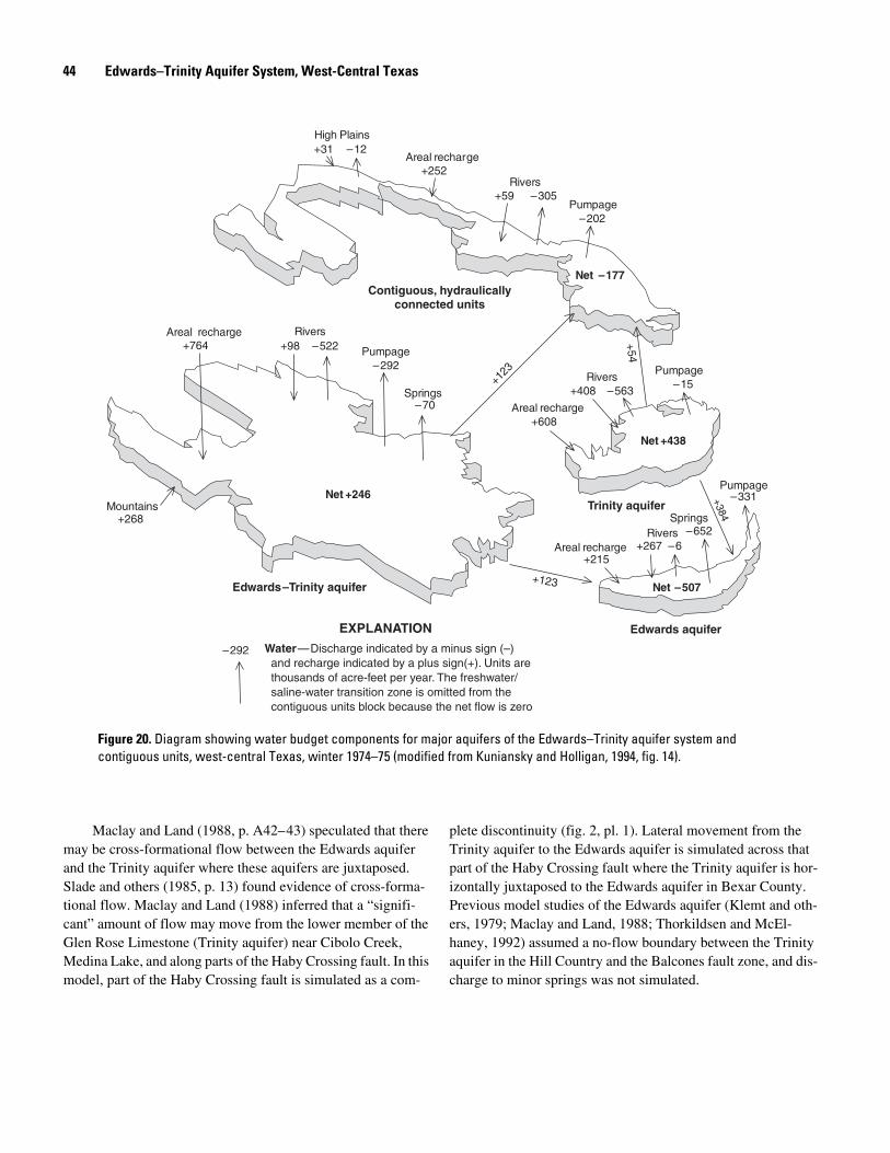
44 Edwards–Trinity Aquifer System, West-Central Texas
Figure 20. Diagram showing water budget components for major aquifers of the Edwards–Trinity aquifer system and contiguous units, west-central Texas, winter 1974–75 (modified from Kuniansky and Holligan, 1994, fig. 14).
Mountains
+764Areal recharge Rivers
Springs
High Plains
+252Areal recharge
Areal recharge+608
Rivers
+215
+123
Areal recharge
+31 –12
+59 –305Pumpage
–202
+268
+98 –522
–70
Pumpage–292
–292
+408 –563
Pumpage –15
+267 –6
Pumpage–331
Springs–652
Rivers
Rivers
Net +246
Net –177
Net +438
Net –507
+123
+54
Contiguous, hydraulicallyconnected units
Edwards–Trinity aquifer
Trinity aquifer
Edwards aquifer
Water—Discharge indicated by a minus sign (–) and recharge indicated by a plus sign(+). Units are thousands of acre-feet per year. The freshwater/ saline-water transition zone is omitted from the contiguous units block because the net flow is zero
EXPLANATION
+384
Maclay and Land (1988, p. A42–43) speculated that there may be cross-formational flow between the Edwards aquifer and the Trinity aquifer where these aquifers are juxtaposed. Slade and others (1985, p. 13) found evidence of cross-forma-tional flow. Maclay and Land (1988) inferred that a “signifi-cant” amount of flow may move from the lower member of the Glen Rose Limestone (Trinity aquifer) near Cibolo Creek, Medina Lake, and along parts of the Haby Crossing fault. In this model, part of the Haby Crossing fault is simulated as a com-
plete discontinuity (fig. 2, pl. 1). Lateral movement from the Trinity aquifer to the Edwards aquifer is simulated across that part of the Haby Crossing fault where the Trinity aquifer is hor-izontally juxtaposed to the Edwards aquifer in Bexar County. Previous model studies of the Edwards aquifer (Klemt and oth-ers, 1979; Maclay and Land, 1988; Thorkildsen and McEl-haney, 1992) assumed a no-flow boundary between the Trinity aquifer in the Hill Country and the Balcones fault zone, and dis-charge to minor springs was not simulated.
Ground-Water Flow 45
Table 4. Simulated and observed springflows for the regional model.[ft, foot; ft3/s, cubic foot per second]
1Ranges in discharge obtained from Brune (1975, 1981), except Barton, Comal, and San Marcos Springs which are gaged.
2Discharge specified in winter 1974–75 simulation.
3Average discharge, water years 1933–89 (Buckner and others, 1989).
4Average discharge, water years 1957–89 (Buckner and others, 1989).
5Average discharge, water years 1918 and 1979–89 (Buckner and others, 1989).
6Estimated discharge for winter 1974–75 (Slade and others, 1986).
7Spring not simulated, winter 1974–75.
SpringPool elevation
above sea level (ft)
Simulated discharge
Observed or estimated discharge1Predevelopment
(ft3/s)Winter 1974–75
(ft3/s)
Comal 623 297.0 2415 Average discharge, 3294 ft3/s;winter 1974–75 discharge, 415 ft3/s
San Felipe 960 60 280 Flow is normally greater than 100 ft3/s
San Marcos 574 167 2241Average discharge, 4166 ft3/s;winter 1974–75 discharge, 241 ft3/s
San Antonio 665 325 88 Flow was greater than 100 ft3/s prior to development, now flow is 10 to 100 ft3/s
Barton 440 40 34 Average discharge, 556 ft3/s;winter 1974–75 discharge, 696 ft3/s
Hueco 655 122 37 Flowed from 10 to 100 ft3/s after development
Las Moras 1,100 19 260 Flowed from 10 to 100 ft3/s
Leona 850 57 25 Flowed from 10 to 100 ft3/s
San Solomon; Giffin 3,320 39 16 Flowed from 10 to 100 ft3/s
Comanche 2,930 18 70 Flowed from 10 to 100 ft3/s
Fort McKavett 2,090 0.3 70 Flowed from 10 to 100 ft3/s
Leon 520 33 70 Flowed from 10 to 100 ft3/s
Cantu 970 4 70 Flowed from 1 to 10 ft3/s
Edge Falls 1,101 6 70 Flowed from 1 to 10 ft3/s
Jacob’s Well 940 6 70 Flowed from 1 to 10 ft3/s
Kickapoo 1,730 5 70 Flowed from 1 to 10 ft3/s
Rebecca 1,020 4 70 Flowed from 1 to 10 ft3/s
Sandia; Saragosa 3,200 26 70 Flowed from 1 to 10 ft3/s
San Pedro 660 74 70 Flowed from 1 to 10 ft3/s
Santa Rosa 2,520 16 70 Flowed from 1 to 10 ft3/s
Schwander 1,116 3 70 Flowed from 1 to 10 ft3/s
Sink 591 9 70 Flowed from 1 to 10 ft3/s
Soldiers Camp 851 44 70 Flowed from 1 to 10 ft3/s
T5 1,960 2 70 Flowed from 1 to 10 ft3/s
Tunas 2,760 30 70 Flowed from 1 to 10 ft3/s
Willow 2,730 16 70 Flowed from 1 to 10 ft3/s
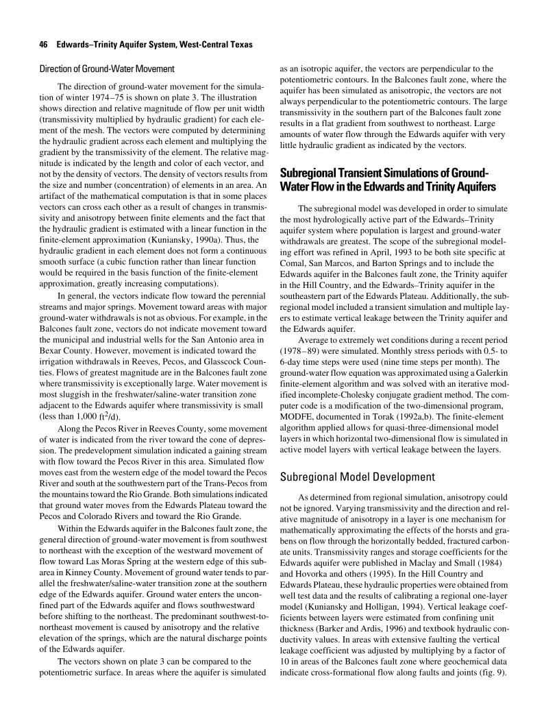
46 Edwards–Trinity Aquifer System, West-Central Texas
Direction of Ground-Water Movement
The direction of ground-water movement for the simula-tion of winter 1974–75 is shown on plate 3. The illustration shows direction and relative magnitude of flow per unit width (transmissivity multiplied by hydraulic gradient) for each ele-ment of the mesh. The vectors were computed by determining the hydraulic gradient across each element and multiplying the gradient by the transmissivity of the element. The relative mag-nitude is indicated by the length and color of each vector, and not by the density of vectors. The density of vectors results from the size and number (concentration) of elements in an area. An artifact of the mathematical computation is that in some places vectors can cross each other as a result of changes in transmis-sivity and anisotropy between finite elements and the fact that the hydraulic gradient is estimated with a linear function in the finite-element approximation (Kuniansky, 1990a). Thus, the hydraulic gradient in each element does not form a continuous smooth surface (a cubic function rather than linear function would be required in the basis function of the finite-element approximation, greatly increasing computations).
In general, the vectors indicate flow toward the perennial streams and major springs. Movement toward areas with major ground-water withdrawals is not as obvious. For example, in the Balcones fault zone, vectors do not indicate movement toward the municipal and industrial wells for the San Antonio area in Bexar County. However, movement is indicated toward the irrigation withdrawals in Reeves, Pecos, and Glasscock Coun-ties. Flows of greatest magnitude are in the Balcones fault zone where transmissivity is exceptionally large. Water movement is most sluggish in the freshwater/saline-water transition zone adjacent to the Edwards aquifer where transmissivity is small (less than 1,000 ft2/d).
Along the Pecos River in Reeves County, some movement of water is indicated from the river toward the cone of depres-sion. The predevelopment simulation indicated a gaining stream with flow toward the Pecos River in this area. Simulated flow moves east from the western edge of the model toward the Pecos River and south at the southwestern part of the Trans-Pecos from the mountains toward the Rio Grande. Both simulations indicated that ground water moves from the Edwards Plateau toward the Pecos and Colorado Rivers and toward the Rio Grande.
Within the Edwards aquifer in the Balcones fault zone, the general direction of ground-water movement is from southwest to northeast with the exception of the westward movement of flow toward Las Moras Spring at the western edge of this sub-area in Kinney County. Movement of ground water tends to par-allel the freshwater/saline-water transition zone at the southern edge of the Edwards aquifer. Ground water enters the uncon-fined part of the Edwards aquifer and flows southwestward before shifting to the northeast. The predominant southwest-to-northeast movement is caused by anisotropy and the relative elevation of the springs, which are the natural discharge points of the Edwards aquifer.
The vectors shown on plate 3 can be compared to the potentiometric surface. In areas where the aquifer is simulated
as an isotropic aquifer, the vectors are perpendicular to the potentiometric contours. In the Balcones fault zone, where the aquifer has been simulated as anisotropic, the vectors are not always perpendicular to the potentiometric contours. The large transmissivity in the southern part of the Balcones fault zone results in a flat gradient from southwest to northeast. Large amounts of water flow through the Edwards aquifer with very little hydraulic gradient as indicated by the vectors.
Subregional Transient Simulations of Ground-Water Flow in the Edwards and Trinity Aquifers
The subregional model was developed in order to simulate the most hydrologically active part of the Edwards–Trinity aquifer system where population is largest and ground-water withdrawals are greatest. The scope of the subregional model-ing effort was refined in April, 1993 to be both site specific at Comal, San Marcos, and Barton Springs and to include the Edwards aquifer in the Balcones fault zone, the Trinity aquifer in the Hill Country, and the Edwards–Trinity aquifer in the southeastern part of the Edwards Plateau. Additionally, the sub-regional model included a transient simulation and multiple lay-ers to estimate vertical leakage between the Trinity aquifer and the Edwards aquifer.
Average to extremely wet conditions during a recent period (1978–89) were simulated. Monthly stress periods with 0.5- to 6-day time steps were used (nine time steps per month). The ground-water flow equation was approximated using a Galerkin finite-element algorithm and was solved with an iterative mod-ified incomplete-Cholesky conjugate gradient method. The com-puter code is a modification of the two-dimensional program, MODFE, documented in Torak (1992a,b). The finite-element algorithm applied allows for quasi-three-dimensional model layers in which horizontal two-dimensional flow is simulated in active model layers with vertical leakage between the layers.
Subregional Model Development
As determined from regional simulation, anisotropy could not be ignored. Varying transmissivity and the direction and rel-ative magnitude of anisotropy in a layer is one mechanism for mathematically approximating the effects of the horsts and gra-bens on flow through the horizontally bedded, fractured carbon-ate units. Transmissivity ranges and storage coefficients for the Edwards aquifer were published in Maclay and Small (1984) and Hovorka and others (1995). In the Hill Country and Edwards Plateau, these hydraulic properties were obtained from well test data and the results of calibrating a regional one-layer model (Kuniansky and Holligan, 1994). Vertical leakage coef-ficients between layers were estimated from confining unit thickness (Barker and Ardis, 1996) and textbook hydraulic con-ductivity values. In areas with extensive faulting the vertical leakage coefficient was adjusted by multiplying by a factor of 10 in areas of the Balcones fault zone where geochemical data indicate cross-formational flow along faults and joints (fig. 9).
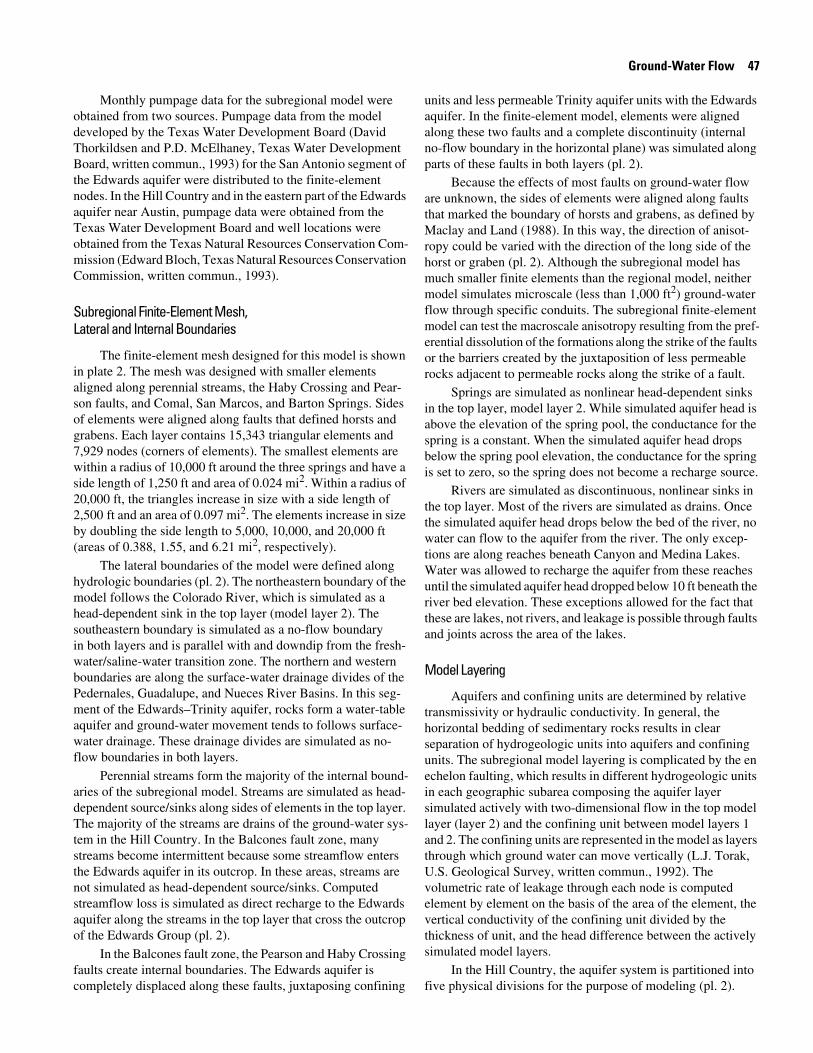
Ground-Water Flow 47
Monthly pumpage data for the subregional model were obtained from two sources. Pumpage data from the model developed by the Texas Water Development Board (David Thorkildsen and P.D. McElhaney, Texas Water Development Board, written commun., 1993) for the San Antonio segment of the Edwards aquifer were distributed to the finite-element nodes. In the Hill Country and in the eastern part of the Edwards aquifer near Austin, pumpage data were obtained from the Texas Water Development Board and well locations were obtained from the Texas Natural Resources Conservation Com-mission (Edward Bloch, Texas Natural Resources Conservation Commission, written commun., 1993).
Subregional Finite-Element Mesh, Lateral and Internal Boundaries
The finite-element mesh designed for this model is shown in plate 2. The mesh was designed with smaller elements aligned along perennial streams, the Haby Crossing and Pear-son faults, and Comal, San Marcos, and Barton Springs. Sides of elements were aligned along faults that defined horsts and grabens. Each layer contains 15,343 triangular elements and 7,929 nodes (corners of elements). The smallest elements are within a radius of 10,000 ft around the three springs and have a side length of 1,250 ft and area of 0.024 mi2. Within a radius of 20,000 ft, the triangles increase in size with a side length of 2,500 ft and an area of 0.097 mi2. The elements increase in size by doubling the side length to 5,000, 10,000, and 20,000 ft (areas of 0.388, 1.55, and 6.21 mi2, respectively).
The lateral boundaries of the model were defined along hydrologic boundaries (pl. 2). The northeastern boundary of the model follows the Colorado River, which is simulated as a head-dependent sink in the top layer (model layer 2). The southeastern boundary is simulated as a no-flow boundary in both layers and is parallel with and downdip from the fresh-water/saline-water transition zone. The northern and western boundaries are along the surface-water drainage divides of the Pedernales, Guadalupe, and Nueces River Basins. In this seg-ment of the Edwards–Trinity aquifer, rocks form a water-table aquifer and ground-water movement tends to follows surface-water drainage. These drainage divides are simulated as no-flow boundaries in both layers.
Perennial streams form the majority of the internal bound-aries of the subregional model. Streams are simulated as head-dependent source/sinks along sides of elements in the top layer. The majority of the streams are drains of the ground-water sys-tem in the Hill Country. In the Balcones fault zone, many streams become intermittent because some streamflow enters the Edwards aquifer in its outcrop. In these areas, streams are not simulated as head-dependent source/sinks. Computed streamflow loss is simulated as direct recharge to the Edwards aquifer along the streams in the top layer that cross the outcrop of the Edwards Group (pl. 2).
In the Balcones fault zone, the Pearson and Haby Crossing faults create internal boundaries. The Edwards aquifer is completely displaced along these faults, juxtaposing confining
units and less permeable Trinity aquifer units with the Edwards aquifer. In the finite-element model, elements were aligned along these two faults and a complete discontinuity (internal no-flow boundary in the horizontal plane) was simulated along parts of these faults in both layers (pl. 2).
Because the effects of most faults on ground-water flow are unknown, the sides of elements were aligned along faults that marked the boundary of horsts and grabens, as defined by Maclay and Land (1988). In this way, the direction of anisot-ropy could be varied with the direction of the long side of the horst or graben (pl. 2). Although the subregional model has much smaller finite elements than the regional model, neither model simulates microscale (less than 1,000 ft2) ground-water flow through specific conduits. The subregional finite-element model can test the macroscale anisotropy resulting from the pref-erential dissolution of the formations along the strike of the faults or the barriers created by the juxtaposition of less permeable rocks adjacent to permeable rocks along the strike of a fault.
Springs are simulated as nonlinear head-dependent sinks in the top layer, model layer 2. While simulated aquifer head is above the elevation of the spring pool, the conductance for the spring is a constant. When the simulated aquifer head drops below the spring pool elevation, the conductance for the spring is set to zero, so the spring does not become a recharge source.
Rivers are simulated as discontinuous, nonlinear sinks in the top layer. Most of the rivers are simulated as drains. Once the simulated aquifer head drops below the bed of the river, no water can flow to the aquifer from the river. The only excep-tions are along reaches beneath Canyon and Medina Lakes. Water was allowed to recharge the aquifer from these reaches until the simulated aquifer head dropped below 10 ft beneath the river bed elevation. These exceptions allowed for the fact that these are lakes, not rivers, and leakage is possible through faults and joints across the area of the lakes.
Model Layering
Aquifers and confining units are determined by relative transmissivity or hydraulic conductivity. In general, the horizontal bedding of sedimentary rocks results in clear separation of hydrogeologic units into aquifers and confining units. The subregional model layering is complicated by the en echelon faulting, which results in different hydrogeologic units in each geographic subarea composing the aquifer layer simulated actively with two-dimensional flow in the top model layer (layer 2) and the confining unit between model layers 1 and 2. The confining units are represented in the model as layers through which ground water can move vertically (L.J. Torak, U.S. Geological Survey, written commun., 1992). The volumetric rate of leakage through each node is computed element by element on the basis of the area of the element, the vertical conductivity of the confining unit divided by the thickness of unit, and the head difference between the actively simulated model layers.
In the Hill Country, the aquifer system is partitioned into five physical divisions for the purpose of modeling (pl. 2).
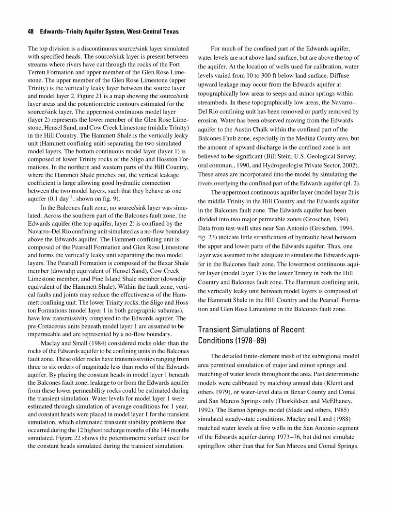
48 Edwards–Trinity Aquifer System, West-Central Texas
The top division is a discontinuous source/sink layer simulated with specified heads. The source/sink layer is present between streams where rivers have cut through the rocks of the Fort Terrett Formation and upper member of the Glen Rose Lime-stone. The upper member of the Glen Rose Limestone (upper Trinity) is the vertically leaky layer between the source layer and model layer 2. Figure 21 is a map showing the source/sink layer areas and the potentiometric contours estimated for the source/sink layer. The uppermost continuous model layer (layer 2) represents the lower member of the Glen Rose Lime-stone, Hensel Sand, and Cow Creek Limestone (middle Trinity) in the Hill Country. The Hammett Shale is the vertically leaky unit (Hammett confining unit) separating the two simulated model layers. The bottom continuous model layer (layer 1) is composed of lower Trinity rocks of the Sligo and Hosston For-mations. In the northern and western parts of the Hill Country, where the Hammett Shale pinches out, the vertical leakage coefficient is large allowing good hydraulic connection between the two model layers, such that they behave as one aquifer (0.1 day-1, shown on fig. 9).
In the Balcones fault zone, no source/sink layer was simu-lated. Across the southern part of the Balcones fault zone, the Edwards aquifer (the top aquifer, layer 2) is confined by the Navarro–Del Rio confining unit simulated as a no-flow boundary above the Edwards aquifer. The Hammett confining unit is composed of the Pearsall Formation and Glen Rose Limestone and forms the vertically leaky unit separating the two model layers. The Pearsall Formation is composed of the Bexar Shale member (downdip equivalent of Hensel Sand), Cow Creek Limestone member, and Pine Island Shale member (downdip equivalent of the Hammett Shale). Within the fault zone, verti-cal faults and joints may reduce the effectiveness of the Ham-mett confining unit. The lower Trinity rocks, the Sligo and Hoss-ton Formations (model layer 1 in both geographic subareas), have low transmissivity compared to the Edwards aquifer. The pre-Cretaceous units beneath model layer 1 are assumed to be impermeable and are represented by a no-flow boundary.
Maclay and Small (1984) considered rocks older than the rocks of the Edwards aquifer to be confining units in the Balcones fault zone. These older rocks have transmissivities ranging from three to six orders of magnitude less than rocks of the Edwards aquifer. By placing the constant heads in model layer 1 beneath the Balcones fault zone, leakage to or from the Edwards aquifer from these lower permeability rocks could be estimated during the transient simulation. Water levels for model layer 1 were estimated through simulation of average conditions for 1 year, and constant heads were placed in model layer 1 for the transient simulation, which eliminated transient stability problems that occurred during the 12 highest recharge months of the 144 months simulated. Figure 22 shows the potentiometric surface used for the constant heads simulated during the transient simulation.
For much of the confined part of the Edwards aquifer,
water levels are not above land surface, but are above the top of
the aquifer. At the location of wells used for calibration, water levels varied from 10 to 300 ft below land surface. Diffuse
upward leakage may occur from the Edwards aquifer at
topographically low areas to seeps and minor springs within
streambeds. In these topographically low areas, the Navarro–
Del Rio confining unit has been removed or partly removed by
erosion. Water has been observed moving from the Edwards
aquifer to the Austin Chalk within the confined part of the Balcones Fault zone, especially in the Medina County area, but
the amount of upward discharge in the confined zone is not
believed to be significant (Bill Stein, U.S. Geological Survey,
oral commun., 1990, and Hydrogeologist Private Sector, 2002).
These areas are incorporated into the model by simulating the
rivers overlying the confined part of the Edwards aquifer (pl. 2).
The uppermost continuous aquifer layer (model layer 2) is
the middle Trinity in the Hill Country and the Edwards aquifer
in the Balcones fault zone. The Edwards aquifer has been
divided into two major permeable zones (Groschen, 1994). Data from test-well sites near San Antonio (Groschen, 1994,
fig. 23) indicate little stratification of hydraulic head between
the upper and lower parts of the Edwards aquifer. Thus, one
layer was assumed to be adequate to simulate the Edwards aqui-
fer in the Balcones fault zone. The lowermost continuous aqui-
fer layer (model layer 1) is the lower Trinity in both the Hill
Country and Balcones fault zone. The Hammett confining unit, the vertically leaky unit between model layers is composed of
the Hammett Shale in the Hill Country and the Pearsall Forma-
tion and Glen Rose Limestone in the Balcones fault zone.
Transient Simulations of Recent Conditions (1978–89)
The detailed finite-element mesh of the subregional model
area permitted simulation of major and minor springs and
matching of water levels throughout the area. Past deterministic
models were calibrated by matching annual data (Klemt and
others 1979), or water-level data in Bexar County and Comal
and San Marcos Springs only (Thorkildsen and McElhaney, 1992). The Barton Springs model (Slade and others, 1985)
simulated steady-state conditions. Maclay and Land (1988)
matched water levels at five wells in the San Antonio segment
of the Edwards aquifer during 1973–76, but did not simulate
springflow other than that for San Marcos and Comal Springs.
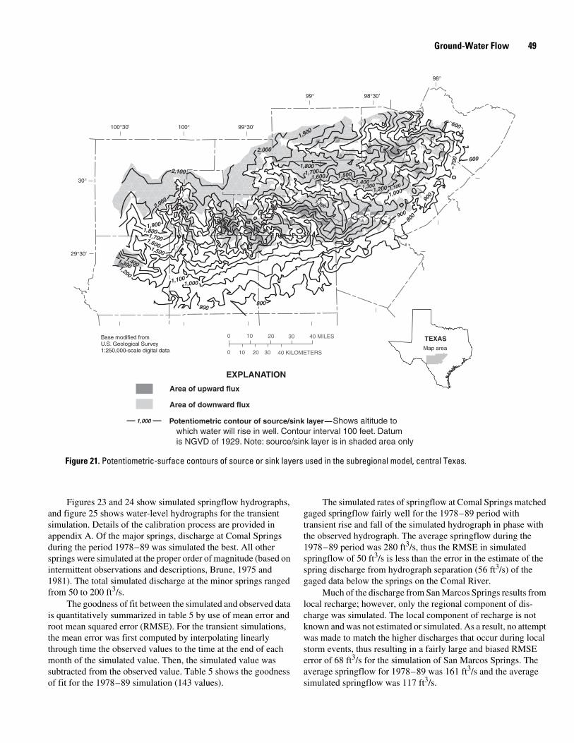
Ground-Water Flow 49
Figure 21. Potentiometric-surface contours of source or sink layers used in the subregional model, central Texas.
EXPLANATION
Potentiometric contour of source/sink layer—Shows altitude to which water will rise in well. Contour interval 100 feet. Datum is NGVD of 1929. Note: source/sink layer is in shaded area only
Area of upward flux
Area of downward flux
Base modified from U.S. Geological Survey1:250,000-scale digital data
0 10 20 30 40 MILES
0 10 20 30 40 KILOMETERS
TEXASMap area
98°
99° 98°30'
99°30'100°30'
29°30'
100°
30°
2,100
2,000
1,9001,800
1,7001,6001,500
1,100
1,200
1,3001,400
1,000
900800
800
600
600
900
1,000
2,000
1,8001,700
1,700
1,600
1,200 1,1001,3001,400
1,500
1,900
1,00090
0
700
Figures 23 and 24 show simulated springflow hydrographs, and figure 25 shows water-level hydrographs for the transient simulation. Details of the calibration process are provided in appendix A. Of the major springs, discharge at Comal Springs during the period 1978–89 was simulated the best. All other springs were simulated at the proper order of magnitude (based on intermittent observations and descriptions, Brune, 1975 and 1981). The total simulated discharge at the minor springs ranged from 50 to 200 ft3/s.
The goodness of fit between the simulated and observed data is quantitatively summarized in table 5 by use of mean error and root mean squared error (RMSE). For the transient simulations, the mean error was first computed by interpolating linearly through time the observed values to the time at the end of each month of the simulated value. Then, the simulated value was subtracted from the observed value. Table 5 shows the goodness of fit for the 1978–89 simulation (143 values).
The simulated rates of springflow at Comal Springs matched gaged springflow fairly well for the 1978–89 period with transient rise and fall of the simulated hydrograph in phase with the observed hydrograph. The average springflow during the 1978–89 period was 280 ft3/s, thus the RMSE in simulated springflow of 50 ft3/s is less than the error in the estimate of the spring discharge from hydrograph separation (56 ft3/s) of the gaged data below the springs on the Comal River.
Much of the discharge from San Marcos Springs results from local recharge; however, only the regional component of dis-charge was simulated. The local component of recharge is not known and was not estimated or simulated. As a result, no attempt was made to match the higher discharges that occur during local storm events, thus resulting in a fairly large and biased RMSE error of 68 ft3/s for the simulation of San Marcos Springs. The average springflow for 1978–89 was 161 ft3/s and the average simulated springflow was 117 ft3/s.
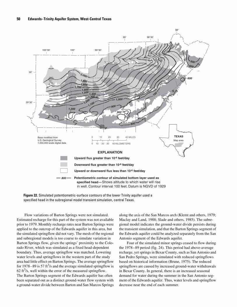
50 Edwards–Trinity Aquifer System, West-Central Texas
Figure 22. Simulated potentiometric-surface contours of the lower Trinity aquifer used a specified head in the subregional model transient simulation, central Texas.
2,000
1,9001,800
1,7001,6001,500
1,4001,300
1,200
1,1001,000
900
800
700
900
600
600
500
700
1,200
98°
99° 98°30'
99°30'100°30'
29°30'
100°
30°
TEXASMap area
Base modified from U.S. Geological Survey1:250,000-scale digital data
0 10 20 30 40 MILES
0 10 20 30 40 KILOMETERS
EXPLANATION
800 Potentiometric contour of simulated bottom layer used as specified head—Shows altitude to which water will rise in well. Contour interval 100 feet. Datum is NGVD of 1929
Upward flux greater than 10-6 feet/day
Downward flux greater than 10-6 feet/day
Upward or downward flux less than 10-6 feet/day
Flow variations of Barton Springs were not simulated. Estimated recharge for this part of the system was not available prior to 1979. Monthly recharge rates near Barton Springs were applied to the outcrop of the Edwards aquifer in this area, but the simulated springflow did not vary. The mesh of the regional and subregional models is too coarse to simulate variation in Barton Springs flow, given the springs’ proximity to the Colo-rado River, which was simulated as a fixed head-dependent boundary. Thus, average springflow was matched. Lowering water levels and springflows in the western part of the study area had little effect on Barton Springs. The average springflow for 1978–89 is 57 ft3/s and the average simulated springflow is 62 ft3/s, well within the error of the measured springflow. The Barton Springs segment of the Edwards aquifer has often been separated out as a distinct ground-water flow system with a ground-water divide between Barton and San Marcos Springs
along the axis of the San Marcos arch (Klemt and others, 1979; Maclay and Land, 1988; Slade and others, 1985). The subre-gional model indicates the ground-water divide persists during the transient simulation, and that the Barton Springs segment of the Edwards aquifer could be analyzed separately from the San Antonio segment of the Edwards aquifer.
Four of the simulated minor springs ceased to flow during the 1978–89 period (fig. 24). This period had above-average recharge, yet springs in Bexar County, such as San Antonio and San Pedro Springs, were simulated with reduced springflows based on historical information (Brune, 1975). The reduced springflows are caused by increased ground-water withdrawals in Bexar County. In general, there is an increased seasonal demand for water during the summer in the San Antonio seg-ment of the Edwards aquifer. Thus, water levels and springflow decrease near the end of each summer.
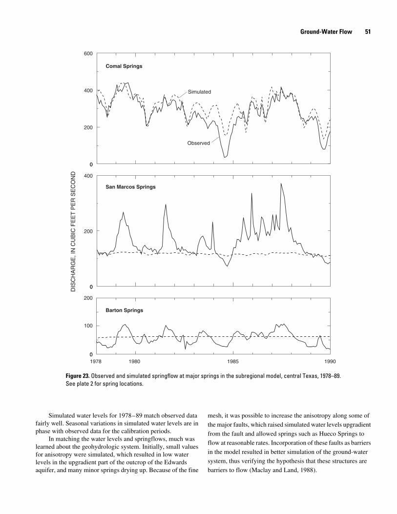
Ground-Water Flow 51
Figure 23. Observed and simulated springflow at major springs in the subregional model, central Texas, 1978–89. See plate 2 for spring locations.
0
600
0
200
400
0
400
0
200
0
200
0
100
1978 19901980 1985
Comal Springs
San Marcos Springs
Barton Springs
DIS
CH
AR
GE
, IN
CU
BIC
FE
ET
PE
R S
EC
ON
D
Simulated
Observed
Simulated water levels for 1978–89 match observed data fairly well. Seasonal variations in simulated water levels are in phase with observed data for the calibration periods.
In matching the water levels and springflows, much was learned about the geohydrologic system. Initially, small values for anisotropy were simulated, which resulted in low water levels in the upgradient part of the outcrop of the Edwards aquifer, and many minor springs drying up. Because of the fine
mesh, it was possible to increase the anisotropy along some of
the major faults, which raised simulated water levels upgradient
from the fault and allowed springs such as Hueco Springs to
flow at reasonable rates. Incorporation of these faults as barriers
in the model resulted in better simulation of the ground-water
system, thus verifying the hypothesis that these structures are
barriers to flow (Maclay and Land, 1988).
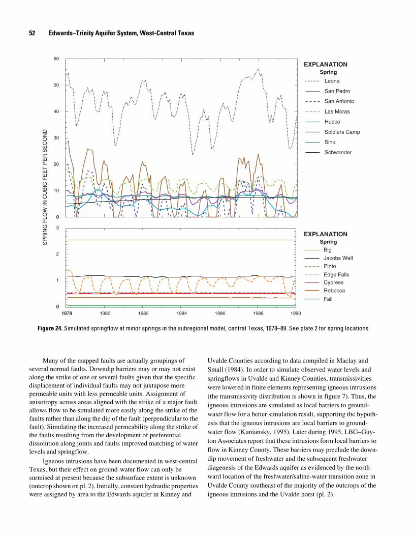
52 Edwards–Trinity Aquifer System, West-Central Texas
Figure 24. Simulated springflow at minor springs in the subregional model, central Texas, 1978–89. See plate 2 for spring locations.
0
60
0
10
20
30
40
50
SP
RIN
G F
LOW
IN C
UB
IC F
EE
T P
ER
SE
CO
ND
Hueco
Las Moras
Leona
San Antonio
San Pedro
Sink
Soldiers Camp
Schwander
1978 19901978 1980 1982 1984 1986 19880
3
0
1
2
EXPLANATION
CypressEdge Falls
Big
Spring
EXPLANATIONSpring
Fall
Jacobs Well
Pinto
Rebecca
Many of the mapped faults are actually groupings of several normal faults. Downdip barriers may or may not exist along the strike of one or several faults given that the specific displacement of individual faults may not juxtapose more permeable units with less permeable units. Assignment of anisotropy across areas aligned with the strike of a major fault allows flow to be simulated more easily along the strike of the faults rather than along the dip of the fault (perpendicular to the fault). Simulating the increased permeability along the strike of the faults resulting from the development of preferential dissolution along joints and faults improved matching of water levels and springflow.
Igneous intrusions have been documented in west-central Texas, but their effect on ground-water flow can only be surmised at present because the subsurface extent is unknown (outcrop shown on pl. 2). Initially, constant hydraulic properties were assigned by area to the Edwards aquifer in Kinney and
Uvalde Counties according to data compiled in Maclay and Small (1984). In order to simulate observed water levels and springflows in Uvalde and Kinney Counties, transmissivities were lowered in finite elements representing igneous intrusions (the transmissivity distribution is shown in figure 7). Thus, the igneous intrusions are simulated as local barriers to ground-water flow for a better simulation result, supporting the hypoth-esis that the igneous intrusions are local barriers to ground-water flow (Kuniansky, 1995). Later during 1995, LBG–Guy-ton Associates report that these intrusions form local barriers to flow in Kinney County. These barriers may preclude the down-dip movement of freshwater and the subsequent freshwater diagenesis of the Edwards aquifer as evidenced by the north-ward location of the freshwater/saline-water transition zone in Uvalde County southeast of the majority of the outcrops of the igneous intrusions and the Uvalde horst (pl. 2).
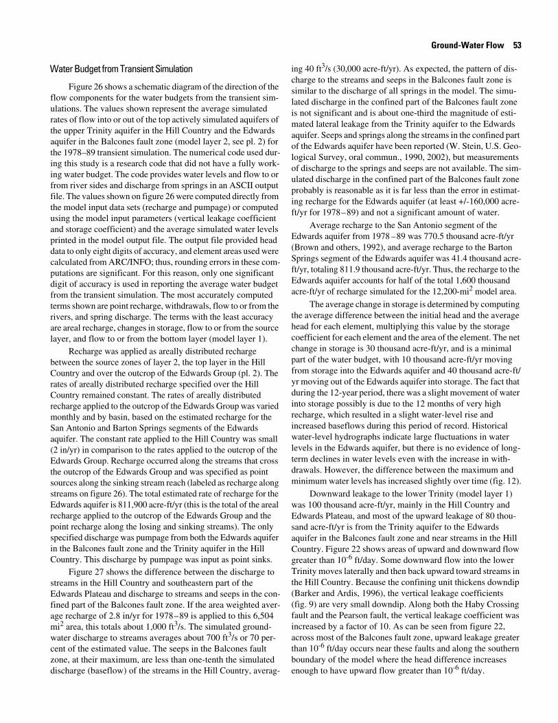
Ground-Water Flow 53
Water Budget from Transient Simulation
Figure 26 shows a schematic diagram of the direction of the flow components for the water budgets from the transient sim-ulations. The values shown represent the average simulated rates of flow into or out of the top actively simulated aquifers of the upper Trinity aquifer in the Hill Country and the Edwards aquifer in the Balcones fault zone (model layer 2, see pl. 2) for the 1978–89 transient simulation. The numerical code used dur-ing this study is a research code that did not have a fully work-ing water budget. The code provides water levels and flow to or from river sides and discharge from springs in an ASCII output file. The values shown on figure 26 were computed directly from the model input data sets (recharge and pumpage) or computed using the model input parameters (vertical leakage coefficient and storage coefficient) and the average simulated water levels printed in the model output file. The output file provided head data to only eight digits of accuracy, and element areas used were calculated from ARC/INFO; thus, rounding errors in these com-putations are significant. For this reason, only one significant digit of accuracy is used in reporting the average water budget from the transient simulation. The most accurately computed terms shown are point recharge, withdrawals, flow to or from the rivers, and spring discharge. The terms with the least accuracy are areal recharge, changes in storage, flow to or from the source layer, and flow to or from the bottom layer (model layer 1).
Recharge was applied as areally distributed recharge between the source zones of layer 2, the top layer in the Hill Country and over the outcrop of the Edwards Group (pl. 2). The rates of areally distributed recharge specified over the Hill Country remained constant. The rates of areally distributed recharge applied to the outcrop of the Edwards Group was varied monthly and by basin, based on the estimated recharge for the San Antonio and Barton Springs segments of the Edwards aquifer. The constant rate applied to the Hill Country was small (2 in/yr) in comparison to the rates applied to the outcrop of the Edwards Group. Recharge occurred along the streams that cross the outcrop of the Edwards Group and was specified as point sources along the sinking stream reach (labeled as recharge along streams on figure 26). The total estimated rate of recharge for the Edwards aquifer is 811,900 acre-ft/yr (this is the total of the areal recharge applied to the outcrop of the Edwards Group and the point recharge along the losing and sinking streams). The only specified discharge was pumpage from both the Edwards aquifer in the Balcones fault zone and the Trinity aquifer in the Hill Country. This discharge by pumpage was input as point sinks.
Figure 27 shows the difference between the discharge to streams in the Hill Country and southeastern part of the Edwards Plateau and discharge to streams and seeps in the con-fined part of the Balcones fault zone. If the area weighted aver-age recharge of 2.8 in/yr for 1978–89 is applied to this 6,504 mi2 area, this totals about 1,000 ft3/s. The simulated ground-water discharge to streams averages about 700 ft3/s or 70 per-cent of the estimated value. The seeps in the Balcones fault zone, at their maximum, are less than one-tenth the simulated discharge (baseflow) of the streams in the Hill Country, averag-
ing 40 ft3/s (30,000 acre-ft/yr). As expected, the pattern of dis-charge to the streams and seeps in the Balcones fault zone is similar to the discharge of all springs in the model. The simu-lated discharge in the confined part of the Balcones fault zone is not significant and is about one-third the magnitude of esti-mated lateral leakage from the Trinity aquifer to the Edwards aquifer. Seeps and springs along the streams in the confined part of the Edwards aquifer have been reported (W. Stein, U.S. Geo-logical Survey, oral commun., 1990, 2002), but measurements of discharge to the springs and seeps are not available. The sim-ulated discharge in the confined part of the Balcones fault zone probably is reasonable as it is far less than the error in estimat-ing recharge for the Edwards aquifer (at least +/-160,000 acre-ft/yr for 1978–89) and not a significant amount of water.
Average recharge to the San Antonio segment of the Edwards aquifer from 1978 –89 was 770.5 thousand acre-ft/yr (Brown and others, 1992), and average recharge to the Barton Springs segment of the Edwards aquifer was 41.4 thousand acre-ft/yr, totaling 811.9 thousand acre-ft/yr. Thus, the recharge to the Edwards aquifer accounts for half of the total 1,600 thousand acre-ft/yr of recharge simulated for the 12,200-mi2 model area.
The average change in storage is determined by computing the average difference between the initial head and the average head for each element, multiplying this value by the storage coefficient for each element and the area of the element. The net change in storage is 30 thousand acre-ft/yr, and is a minimal part of the water budget, with 10 thousand acre-ft/yr moving from storage into the Edwards aquifer and 40 thousand acre-ft/yr moving out of the Edwards aquifer into storage. The fact that during the 12-year period, there was a slight movement of water into storage possibly is due to the 12 months of very high recharge, which resulted in a slight water-level rise and increased baseflows during this period of record. Historical water-level hydrographs indicate large fluctuations in water levels in the Edwards aquifer, but there is no evidence of long-term declines in water levels even with the increase in with-drawals. However, the difference between the maximum and minimum water levels has increased slightly over time (fig. 12).
Downward leakage to the lower Trinity (model layer 1) was 100 thousand acre-ft/yr, mainly in the Hill Country and Edwards Plateau, and most of the upward leakage of 80 thou-sand acre-ft/yr is from the Trinity aquifer to the Edwards aquifer in the Balcones fault zone and near streams in the Hill Country. Figure 22 shows areas of upward and downward flow greater than 10-6 ft/day. Some downward flow into the lower Trinity moves laterally and then back upward toward streams in the Hill Country. Because the confining unit thickens downdip (Barker and Ardis, 1996), the vertical leakage coefficients (fig. 9) are very small downdip. Along both the Haby Crossing fault and the Pearson fault, the vertical leakage coefficient was increased by a factor of 10. As can be seen from figure 22, across most of the Balcones fault zone, upward leakage greater than 10-6 ft/day occurs near these faults and along the southern boundary of the model where the head difference increases enough to have upward flow greater than 10-6 ft/day.
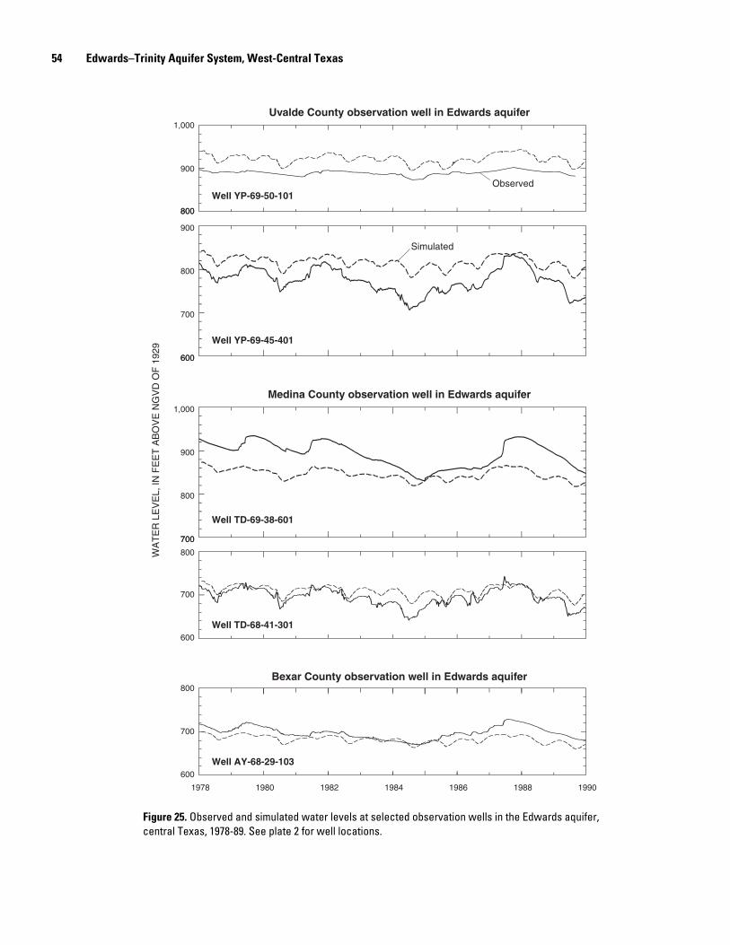
54 Edwards–Trinity Aquifer System, West-Central Texas
Figure 25. Observed and simulated water levels at selected observation wells in the Edwards aquifer, central Texas, 1978-89. See plate 2 for well locations.
800
1,000
800
900
Well YP-69-50-101
600
900
600
700
800
Well YP-69-45-401
700
1,000
700
800
900
Well TD-69-38-601
800
700
19901978 1980 1982 1984 1986 1988
Well TD-68-41-301
800
700
600
600
Well AY-68-29-103
WA
TE
R L
EV
EL,
IN F
EE
T A
BO
VE
NG
VD
OF
192
9
Uvalde County observation well in Edwards aquifer
Medina County observation well in Edwards aquifer
Bexar County observation well in Edwards aquifer
Observed
Simulated
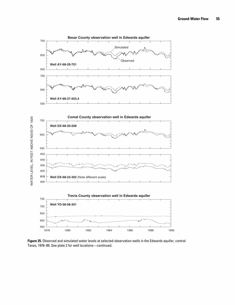
Ground-Water Flow 55
Figure 25. Observed and simulated water levels at selected observation wells in the Edwards aquifer, central Texas, 1978–89. See plate 2 for well locations—continued.
750
550
650
750
550
650
750
550
650
610
640
650
610
600
620
630
650
700
750
550
600
Well AY-68-29-701
Well AY-68-37-203,4
Well DX-68-30-208
Well DX-68-23-302 (Note different scale)
Well YD-58-58-301
Bexar County observation well in Edwards aquifer
Comal County observation well in Edwards aquifer
Travis County observation well in Edwards aquifer
19901978 1980 1982 1984 1986 1988
Observed
Simulated
WA
TE
R L
EV
EL,
IN F
EE
T A
BO
VE
NG
VD
OF
192
9
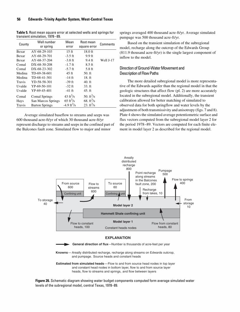
56 Edwards–Trinity Aquifer System, West-Central Texas
Figure 26. Schematic diagram showing water budget components computed form average simulated water levels of the subregional model, central Texas, 1978–89.
Hammett Shale confining unit
Model layer 2
Model layer 1
Knowns—
EXPLANATION
Areally distributed recharge, recharge along streams on Edwards outcrop,and pumpage. Source heads and constant heads
Estimated from simulated heads—Flow to and from source head nodes in top layer and constant head nodes in bottom layer, flow to and from source layer heads, flow to streams and springs, and flow between layers
From source600
Confining unit Confining unit
To storage40
Flow to constantheads, 100
Flow from constantheads, 80
From storage
10
Rechargefrom lakes, 10
Flow to springs400
Pumpage500
Constant heads nodes
Flow tostreams
600
Areallydistributedrecharge
800Point rechargealong streams in the Balcones fault zone, 200To source
60
General direction of flux—Number is thousands of acre-feet per year
Table 5. Root mean square error at selected wells and springs for transient simulation, 1978–89.
Average simulated baseflow to streams and seeps was 600 thousand acre-ft/yr of which 30 thousand acre-ft/yr represent discharge to streams and seeps in the confined part of the Balcones fault zone. Simulated flow to major and minor
springs averaged 400 thousand acre-ft/yr. Average simulated pumpage was 500 thousand acre-ft/yr.
Based on the transient simulation of the subregional model, recharge along the outcrop of the Edwards Group (811.9 thousand acre-ft/yr) is the single largest component of inflow to the model.
Direction of Ground-Water Movement and Description of Flow Paths
The more detailed subregional model is more representa-tive of the Edwards aquifer than the regional model in that the geologic structures that affect flow (pl. 2) are more accurately located in the subregional model. Additionally, the transient calibration allowed for better matching of simulated to observed data for both springflow and water levels by the adjustment of both transmissivity and anisotropy (figs. 7 and 8). Plate 4 shows the simulated average potentiometric surface and flux vectors computed from the subregional model layer 2 for the period 1978–89. Vectors are computed for each finite ele-ment in model layer 2 as described for the regional model.
County Well number or spring
Mean error
Root mean square error Comments
Bexar AY-68-29-103 15 ft 18.0 ftBexar AY-68-29-701 -3.5 ft 9.9 ftBexar AY-68-37-204 -3.8 ft 9.4 ft Well J-17Comal DX-68-30-208 -1.7 ft 8.5 ftComal DX-68-23-302 -5.7 ft 5.8 ftMedina TD-69-38-601 45 ft 50. ftMedina TD-68-41-301 -14 ft 18. ftTravis YD-58-58-301 -39 ft 40. ftUvalde YP-69-50-101 -32 ft 33. ft Uvalde YP-69-45-401 -41 ft 45. ft
Comal Comal Springs 43 ft3/s 50. ft3/sHays San Marcos Springs 65 ft3/s 68. ft3/sTravis Barton Springs -4.9 ft3/s 23. ft3/s
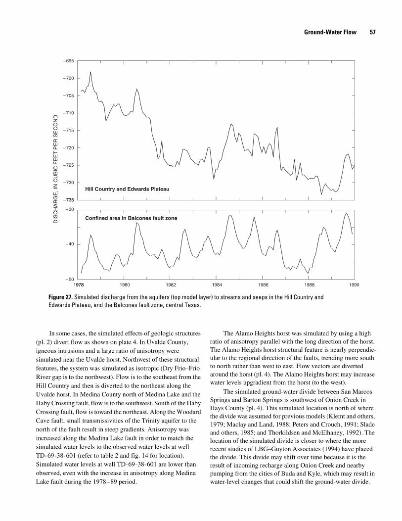
Ground-Water Flow 57
Figure 27. Simulated discharge from the aquifers (top model layer) to streams and seeps in the Hill Country and Edwards Plateau, and the Balcones fault zone, central Texas.
735
–695
–735
–730
–725
–720
–715
–710
–705
–700
1978 19901978 1980 1982 1984 1986 1988
–30
–50
–40
DIS
CH
AR
GE
, IN
CU
BIC
FE
ET
PE
R S
EC
ON
D
Hill Country and Edwards Plateau
Confined area in Balcones fault zone
In some cases, the simulated effects of geologic structures (pl. 2) divert flow as shown on plate 4. In Uvalde County, igneous intrusions and a large ratio of anisotropy were simulated near the Uvalde horst. Northwest of these structural features, the system was simulated as isotropic (Dry Frio–Frio River gap is to the northwest). Flow is to the southeast from the Hill Country and then is diverted to the northeast along the Uvalde horst. In Medina County north of Medina Lake and the Haby Crossing fault, flow is to the southwest. South of the Haby Crossing fault, flow is toward the northeast. Along the Woodard Cave fault, small transmissivities of the Trinity aquifer to the north of the fault result in steep gradients. Anisotropy was increased along the Medina Lake fault in order to match the simulated water levels to the observed water levels at well TD-69-38-601 (refer to table 2 and fig. 14 for location). Simulated water levels at well TD-69-38-601 are lower than observed, even with the increase in anisotropy along Medina Lake fault during the 1978–89 period.
The Alamo Heights horst was simulated by using a high ratio of anisotropy parallel with the long direction of the horst. The Alamo Heights horst structural feature is nearly perpendic-ular to the regional direction of the faults, trending more south to north rather than west to east. Flow vectors are diverted around the horst (pl. 4). The Alamo Heights horst may increase water levels upgradient from the horst (to the west).
The simulated ground-water divide between San Marcos Springs and Barton Springs is southwest of Onion Creek in Hays County (pl. 4). This simulated location is north of where the divide was assumed for previous models (Klemt and others, 1979; Maclay and Land, 1988; Peters and Crouch, 1991; Slade and others, 1985; and Thorkildsen and McElhaney, 1992). The location of the simulated divide is closer to where the more recent studies of LBG–Guyton Associates (1994) have placed the divide. This divide may shift over time because it is the result of incoming recharge along Onion Creek and nearby pumping from the cities of Buda and Kyle, which may result in water-level changes that could shift the ground-water divide.
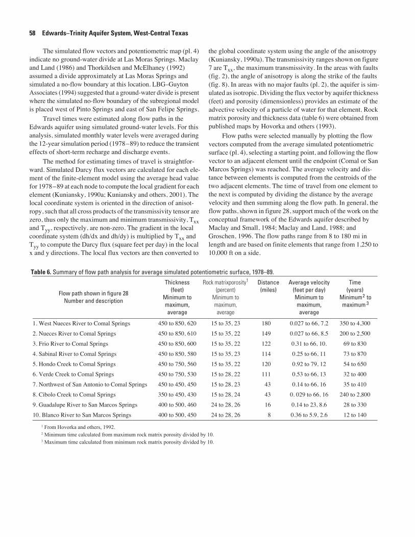
58 Edwards–Trinity Aquifer System, West-Central Texas
The simulated flow vectors and potentiometric map (pl. 4) indicate no ground-water divide at Las Moras Springs. Maclay and Land (1986) and Thorkildsen and McElhaney (1992) assumed a divide approximately at Las Moras Springs and simulated a no-flow boundary at this location. LBG–Guyton Associates (1994) suggested that a ground-water divide is present where the simulated no-flow boundary of the subregional model is placed west of Pinto Springs and east of San Felipe Springs.
Travel times were estimated along flow paths in the Edwards aquifer using simulated ground-water levels. For this analysis, simulated monthly water levels were averaged during the 12-year simulation period (1978–89) to reduce the transient effects of short-term recharge and discharge events.
The method for estimating times of travel is straightfor-ward. Simulated Darcy flux vectors are calculated for each ele-ment of the finite-element model using the average head value for 1978–89 at each node to compute the local gradient for each element (Kuniansky, 1990a; Kuniansky and others, 2001). The local coordinate system is oriented in the direction of anisot-ropy, such that all cross products of the transmissivity tensor are zero, thus only the maximum and minimum transmissivity, Txx and Tyy, respectively, are non-zero. The gradient in the local coordinate system (dh/dx and dh/dy) is multiplied by Txx and Tyy to compute the Darcy flux (square feet per day) in the local x and y directions. The local flux vectors are then converted to
the global coordinate system using the angle of the anisotropy (Kuniansky, 1990a). The transmissivity ranges shown on figure 7 are Txx, the maximum transmissivity. In the areas with faults (fig. 2), the angle of anisotropy is along the strike of the faults (fig. 8). In areas with no major faults (pl. 2), the aquifer is sim-ulated as isotropic. Dividing the flux vector by aquifer thickness (feet) and porosity (dimensionless) provides an estimate of the advective velocity of a particle of water for that element. Rock matrix porosity and thickness data (table 6) were obtained from published maps by Hovorka and others (1993).
Flow paths were selected manually by plotting the flow vectors computed from the average simulated potentiometric surface (pl. 4), selecting a starting point, and following the flow vector to an adjacent element until the endpoint (Comal or San Marcos Springs) was reached. The average velocity and dis-tance between elements is computed from the centroids of the two adjacent elements. The time of travel from one element to the next is computed by dividing the distance by the average velocity and then summing along the flow path. In general, the flow paths, shown in figure 28, support much of the work on the conceptual framework of the Edwards aquifer described by Maclay and Small, 1984; Maclay and Land, 1988; and Groschen, 1996. The flow paths range from 8 to 180 mi in length and are based on finite elements that range from 1,250 to 10,000 ft on a side.
Table 6. Summary of flow path analysis for average simulated potentiometric surface, 1978–89.
Flow path shown in figure 28Number and description
Thickness (feet)
Minimum to maximum, average
Rock matrixporosity1 (percent)
Minimum to maximum, average
Distance (miles)
Average velocity (feet per day) Minimum to maximum, average
Time (years)
Minimum2 to maximum 3
1. West Nueces River to Comal Springs 450 to 850, 620 15 to 35, 23 180 0.027 to 66, 7.2 350 to 4,300
2. Nueces River to Comal Springs 450 to 850, 610 15 to 35, 22 149 0.027 to 66, 8.5 200 to 2,500
3. Frio River to Comal Springs 450 to 850, 600 15 to 35, 22 122 0.31 to 66, 10. 69 to 830
4. Sabinal River to Comal Springs 450 to 850, 580 15 to 35, 23 114 0.25 to 66, 11 73 to 870
5. Hondo Creek to Comal Springs 450 to 750, 560 15 to 35, 22 120 0.92 to 79, 12 54 to 650
6. Verde Creek to Comal Springs 450 to 750, 530 15 to 28, 22 111 0.53 to 66, 13 32 to 400
7. Northwest of San Antonio to Comal Springs 450 to 450, 450 15 to 28, 23 43 0.14 to 66, 16 35 to 410
8. Cibolo Creek to Comal Springs 350 to 450, 430 15 to 28, 24 43 0. 029 to 66, 16 240 to 2,800
9. Guadalupe River to San Marcos Springs 400 to 500, 460 24 to 28, 26 16 0.14 to 23, 8.6 28 to 330
10. Blanco River to San Marcos Springs 400 to 500, 450 24 to 28, 26 8 0.36 to 5.9, 2.6 12 to 140
1 From Hovorka and others, 1992.2 Minimum time calculated from maximum rock matrix porosity divided by 10.3 Maximum time calculated from minimum rock matrix porosity divided by 10.
Ground-Water Flow 59
Figure 28. Selected flow paths from the subregional model, central Texas (modified from Kuniansky and others, 2001).
San Antonio
Austin
West
Rio
Grande
N
uecesR N
uecesR
iver
Frio
Sabinal
Medina
Guadalupe River
Pedernales River
Cibolo
Barton Cr
Creek
River
River
Blanco River
Colorado
River
SanAntonioRiver
River
98°
99° 98°30'
99°30'100°30'
29°30'
100°
30°
1
2 34
56
7
8
9
10
Las MorasSprings
Leona Springs
San Antonio Springs
Hueco Springs
Comal Springs
San Marcos Springs
Barton Springs
0 10 20 30
0 10 20 30
Base modified from U.S. Geological Survey1:250,000-scale digital data
Outcrop of the Edwards Group
Selected flow path and number—See table 6
Model boundary
Northern extent of Hammett Shale
Spring
EXPLANATION
1
40 MILES
40 KILOMETERS
TEXASMap area
Estimates of travel times were computed from aquifer thickness and rock matrix porosities within known or inferred ranges from 350 to 850 ft and 15 to 35 percent, respectively (table 6). Computations involving total aquifer thickness and maximum rock matrix porosity, yield maximum travel times. In a karst system, such as the Edwards–Trinity aquifer system, the entire thickness of the aquifer may not be the permeable or transmissive zone. Additionally, the rock matrix porosity may not be representative of the effective porosity (hydraulically connected void spaces). Effective aquifer thickness and effec-tive porosity can be highly variable and is not well defined throughout most of the aquifer. For example, Small and Maclay (1982) report an effective porosity of less than 3 percent for parts of the Edwards aquifer; Sieh (1975) reports effective porosity of less than 1 percent for parts of the Edwards aquifer; Hovorka and others (1993) report effective porosities as low as 5 percent. The minimum rock matrix porosity for each element (range along flow path, table 6) was divided by 10 to estimate
an effective porosity and thus a minimum travel time. Travel times range from 12 to 140 years for a flow path from the Blanco River Basin to San Marcos Springs and from 350 to 4,300 years for a flow path from the West Nueces River Basin to Comal Springs. Minimum travel-time estimates are similar in magnitude to the estimates of the age of the water at these springs determined from tritium isotopes in water (Pearson and Rettman, 1976; Pearson and others, 1975). This supports the hypothesis that the effective porosity and effective thickness of the aquifer probably are less than the respective range (table 6).
Various authors used the tritium data of Pearson and Rett-man (1976) to interpret ages for the waters of the Edwards aqui-fer. Campana and Mahin (1985) used a discrete state compart-ment model to describe the observed tritium concentrations. The discrete state compartment model assumes that water moves from one cell to another as a discrete unit, then mixes completely with water within that cell. Calculated ages were determined to range from 47 to 132 years from Uvalde County,
60 Edwards–Trinity Aquifer System, West-Central Texas
57 to 123 years from Medina County, and 38 to 123 years from Bexar County. The estimated average age of water was 91 years from Comal Springs and 16 years from San Marcos Springs. More recently, Shevenell (1990) used two hydrologic models, well-mixed and piston flow, to describe observed tritium con-centrations. These two end-member hydrologic models allow determination of interpreted minimum and maximum age dates for observed tritium concentrations. The well-mixed model indicated water from Uvalde County was from 96 to 187 years old, Comal Springs water was from 318 to 521 years old, and San Marcos Springs water was from 61 to 75 years old. The piston-flow model indicated Uvalde County water was from 12.5 to 17.9 years old, Comal Springs water was from 14.5 to 17.5 years old, and San Marcos Springs water was from 10.5 to 15 years old.
The estimated ages obtained from the well-mixed model (Shevenell, 1990) agree more closely with the numerical model than with the other hydrogeochemical models. In general, both the subregional finite-element model estimates and the geochemical models indicate that the waters obtained from Comal Springs are a mixture of waters older than those obtained from San Marcos Springs.
The flux vector analysis also was used to estimate the lat-eral flow of water from the lower permeability rocks in the downdip part of the Edwards Group rocks into the higher per-meability rocks in the Edwards aquifer (model layer 2). This estimate was accomplished by computing the perpendicular component of the average flux vectors (1978–89) along the sides of finite-elements that form the line of low permeability versus high permeability elements in model layer 2 (fig. 7), and along the southern boundary of the Edwards aquifer at the fresh-water/saline-water transition zone. The estimated average flow across this 572-mi boundary into the Edwards aquifer was 20 ft3/s, an extremely small rate of flow. Historical water-qual-ity data indicate that some saline water inflows to the freshwater part of the Edwards aquifer during periods of low water levels in the aquifer (Groschen, 1994), but the amount is small and the direction reverses when water levels rise. The amount of fresh-water (low dissolved solids) recharging the aquifer dominates the water quality of the system. The small amounts of saline water that occasionally move into the Edwards aquifer from the less permeable downdip rocks of the Edwards Group or the poorer quality water from the Trinity aquifer have not resulted in any permanent increases in dissolved solids in water from the Edwards aquifer, and this has not changed the potability of the ground water.
The average estimated lateral movement of water into the Edwards aquifer from the Trinity and Edwards–Trinity aquifers (model layer 2, 1978–89) is about 400 ft3/s along the 194-mi boundary of the geographic subarea defined along element sides (pl. 2). This estimate from the subregional model is 20 percent less than the estimate obtained from the regional model. Like the regional model, most of this lateral flow occurs west of the Haby Crossing fault.
Limitations of the Subregional Model and Flow Path Analysis
In developing a numerical model of an aquifer system, numerous simplifications are required in order to approximate the system mathematically. In this quasi-three-dimensional finite-element model, ground-water flow is simulated as hori-zontal and two-dimensional within two model layers, with ver-tical leakage occurring between layers. Specific conduits are not simulated, but the effective transmissivity estimated by this modeling exercise, while within published ranges, represents an effective transmissivity that allows for simulation of similar gradients and matching estimated baseflows and spring dis-charge. The modified version of the MODFE code (L.J. Torak, U.S. Geological Survey, written commun., 1992) used in this study has not been tested elsewhere; thus, programming errors may exist in the code. Verification of the model code was con-ducted by comparing the results of an equivalent finite-element mesh used to test the steady-state model code used for the regional model (Kuniansky, 1990a) using the MODFLOW (McDonald and Harbaugh, 1988) model; both model codes appear to simulate similar ground-water levels and head-depen-dent flux values. A 20-hour run time to simulate the 1978–89 period, using monthly stress periods, made parameter estima-tion and calibration difficult. Thus, it is likely that the model calibration could be improved. Additionally, the lower layer of the model was simulated as a constant-head layer using the steady-state simulated initial conditions with both layers actively simulated. This conceptualization of the system was incorporated to eliminate transient instability in the solution for head in the lower model layer. Transient instability occurred during efforts to simulate the 12 highest monthly recharge events conducted during 144 monthly stress periods within small areas in the lower model layer (relatively low permeabil-ity Trinity aquifer beneath the outcrop of high permeability Edwards aquifer). The solution for head in the Edwards aquifer did not change as a result of simulating the lower layer as con-stant head rather than actively solving for the lower layer heads during the transient simulation.
With all of the limitations described above, simulated heads, spring flows, and baseflows reasonably matched observed data, and transmissivity values used for the Edwards aquifer fall within the ranges published by Maclay and Small (1984) and Hovorka and others (1995). Thus, the estimated direction of flow and Darcy flux along selected flow paths is considered to be reasonable. The least conclusive aspect of the analysis is associated with estimates of pore-water velocity and times of travel due to the poor understanding of effective aqui-fer thickness or the distribution of effective porosity within the Edwards aquifer. Because the minimum travel times tend to match independently estimated travel times using isotope data, this is further evidence that the subregional model represents flow fairly well in the Edwards aquifer.
Summary and Conclusions 61
SUMMARY AND CONCLUSIONS
The Edwards–Trinity aquifer system was studied as part of the U.S. Geological Survey’s Regional Aquifer-System Analy-sis Program. A major goal of the project is to understand and describe the regional ground-water flow system. Development of ground-water flow models of both the regional system and the more dynamic subregion of the system was accomplished using the finite-element method. A two-dimensional one-layer model was developed for the Edwards–Trinity aquifer system and contiguous, hydraulically connected units in west-central Texas (55,600 square miles). A quasi-three-dimensional, multi-layer, ground-water flow model was applied to the major aqui-fers of the Edwards–Trinity aquifer system in the Hill Country and the Balcones fault zone (12,300 square miles).
The ground-water flow system in most of the study area within the Trans-Pecos and Edwards Plateau can be approxi-mated using a one-layer regional model. In local areas, such as in Pecos and Reeves Counties and in Glasscock, Upton, and Reagan Counties, local ground-water withdrawals exceeded recharge, and drawdown was more than 200 feet. With the decrease in ground-water withdrawals after 1974, water levels have recovered somewhat from these drawdowns. In general, most of the Edwards–Trinity aquifer system in the Trans-Pecos and Edwards Plateau has been static (minimal changes in water levels), as can be seen by comparing potentiometric surfaces from predevelopment and postdevelopment (winter 1974–75).
Water budgets from the regional model indicate that the increase in ground-water withdrawals has captured much of the water that would have discharged to many springs and streams in the Trans-Pecos and Edwards Plateau. The simulated regional water budget indicates lateral movement from the Trinity aquifer in the Edwards Plateau and Hill Country toward the Edwards aquifer in the Balcones fault zone.
The most active part of the ground-water system is the Edwards aquifer in the Balcones fault zone. This karst system is unique owing to its existence in a semiarid area and the geologic structures that control the direction of ground-water movement in the aquifer. Unlike other karst systems dominated by hori-zontal beds with vuggy porosity, the secondary porosity of the Edwards aquifer develops along fractures and faults. The en echelon faulting, horsts, and grabens result in permeable mem-bers horizontally juxtaposed to less permeable units. These faults, horsts, and grabens act as a system of diversions or bar-riers to flow across the strike of the en echelon faults. Because most of the joints are aligned with the strike of the en echelon faults, secondary porosity developed along the strike of the faults. Thus, ground water flows more easily along the strike of the faults or upthrown horsts rather than perpendicular to the strike. These structural features may create diversions within one county and can be perpendicular to the regional direction of the faults, such as the Alamo Heights horst. In general, a pref-erential direction of flow (anisotropy in the horizontal dimen-sion) within the Edwards aquifer is created by the geologic structure and the development of secondary porosity along faults and joints.
Additionally, basaltic igneous rocks occur in Uvalde and Kinney Counties and intrude overlying Cretaceous rocks, locally affecting ground-water flow. Although, the surface outcrops of the igneous intrusions are mapped, the subsurface extents are not known, they may impede lateral movement of ground water. Simulation of observed ground-water levels in Uvalde County was improved when the intrusions were simu-lated as localized areas of reduced transmissivity. These igne-ous intrusions may preclude the downdip movement of fresh-water and the subsequent freshwater diagenesis of the Edwards aquifer as evidenced by the northward location of the freshwa-ter/saline-water transition zone in Uvalde County southeast of the outcrop of the majority of the igneous intrusions and the Uvalde horst.
Both the regional and subregional models indicated lateral movement of ground water from the Trinity aquifer in the Hill Country and the Edwards–Trinity aquifer in the Edwards Plateau to the Edwards aquifer in the Balcones fault zone. The simulated average rate of lateral movement of water to the Edwards aquifer in the Balcones fault zone is about 400 (subregional model estimate) or 500 (regional model estimate) cubic feet per second across a 200-mile length of the northern boundary of the Balcones fault zone from both models. This rate includes downdip movement of water from the lower member of the Glen Rose Limestone, Hensell Sand, and Cow Creek Limestone. The complex series of faults and joints complicates the details of downdip movement of water from the Trinity aquifer in the Hill Country and the Edwards–Trinity aquifer in the Edwards Plateau to the Edwards aquifer in the Balcones fault zone. This estimated average is about 2 or 3 cubic feet per second per mile of boundary, which is equivalent to a low-permeability seepage face with a slow drip of water per square foot of area. Most of the simulated lateral movement is from the Edwards–Trinity aquifer west of the Haby Crossing fault. Only 100 cubic feet per second (90 thousand acre-ft/yr) is from the Trinity aquifer in the Hill Country.
The estimated lateral movement into the freshwater part of the Edwards aquifer (model layer 2, 1978–89) from the saline-water part of the Edwards Group rocks was small, 20 cubic feet per second, across the 572 mile length of this boundary. Histor-ical water-quality data indicate that some inflow of saline water to the freshwater part of the Edwards aquifer occurs during peri-ods of low water levels in the Edwards, but the amount is small and the direction reverses when water levels rise. The amount of freshwater (low dissolved solids) recharging the aquifer dominates the water quality of the system. The observed data indicate that small amounts of saline water that occasionally move into the Edwards aquifer from the less permeable down-dip Edwards Group rocks or the poorer quality water from the Trinity aquifer do not reduce the potability of the water in the Edwards aquifer.
The simulated minor springs (15 springs) in the subre-gional model result in significant discharge, which averaged 100 cubic feet per second and ranged from 50 to 200 cubic feet per second in the transient simulations. The average simulated discharge for Comal, San Marcos, and Barton Springs was
62 Edwards–Trinity Aquifer System, West-Central Texas
500 cubic feet per second. The simulated seeps along streams in the confined zone of the Edwards aquifer resulted in a small amount of discharge, averaging about 30 cubic feet per second in the transient simulations (1978–89).
Although, the subregional model is significantly more detailed than the regional model, neither model simulates microscale (1,000 square feet) ground-water flow through spe-cific conduits. Both models duplicate the macroscale anisotropy resulting from the preferential dissolution of the formations along the strike of the faults.
The ground-water flow equations are based on conserva-tion of mass and energy. The regional and subregional models synthesize the known hydrologic boundaries and geologic structures into a heterogeneous continuum model of the karst ground-water flow system. These models are calibrated on both water levels (representing potential energy) and known dis-charges (representing mass balance).
The regional model water budget mass balance provided water-budget estimates for steady-state, long-term average cli-matic conditions. Water budgets from the regional model indi-cate that the increase in ground-water withdrawals has captured 20 percent of the water that would have naturally discharged to streams and 30 percent of the natural discharge to springs after ground-water development. Induced recharge from streams to the ground-water system increased by 12 percent in the postde-velopment simulation from the predevelopment simulation.
The water budget for the subregional model for heads averaged during the transient 1978–89 period indicates that average recharge to the Edwards aquifer was 800 thousand acre-feet per year, which is about half of the 1,600 thousand acre-feet per year of recharge for the subregional model. The average net change in storage, 30 acre-feet per year, is a mini-mal part of the water budget with 10 thousand acre-feet per year moving into the Edwards aquifer and 40 thousand acre-feet per year moving out of the Edwards aquifer. A total of 100 thousand acre-feet per year of downward leakage to the lower model layer occurs mainly in the Hill Country and Edwards Plateau. Most of the 80 thousand acre-feet per year of upward leakage is from the Trinity aquifer to the Edwards aquifer in the Balcones fault zone, with very small amount of this upward leakage near streams in the Hill Country. Average simulated baseflow to streams and seeps was 600 thousand acre-feet per year of which, 30 thousand acre-feet per year represents discharge to streams and seeps in the confined part of the Balcones fault zone. Simulated flow to major and minor springs averaged 400 thousand acre-feet per year. Average simulated pumpage was 500 thousand acre-feet per year. Based on the transient simula-tion of the subregional model, recharge along the outcrop of the Edwards aquifer dominates the water budget.
The transient subregional modeling effort indicates that the ground-water divide between the San Antonio and the Barton Springs segment of the Edwards aquifer persists throughout the 1978–89 period. These two areas may be simulated separately allowing use of either finite-element or finite-difference methods. Most finite-difference methods require the grid to be aligned to the main orientation of faults in
each region simulated, because the method does not incorporate the full transmissivity tensor into the equation for flow. However, as computer technology improves, models will be able to be developed with more active cells or elements than possible at the time of this simulation effort (1995), and more algorithms will be developed for finite-difference codes.
Upward leakage from the Trinity aquifer to the Edwards aquifer is small and insignificant in comparison to the recharge across the outcrop of the Edwards, pumpage, and spring dis-charge. Thus, the numerical problems encountered in attempt-ing transient simulations of the entire system as in the subre-gional model can be avoided with a more simplified model of the Edwards aquifer, as has been done in the past.
SELECTED REFERENCES
Abbott, P.L., 1973, The Edwards limestones in the Balcones fault zone, south-central Texas: University of Texas at Aus-tin, Ph.D. dissertation, 122 p.
Abbott, P.L., 1975, On the hydrology of the Edwards limestone, south-central Texas: Journal of Hydrology, v. 24, p. 251–269.
Abbott, P.L., 1976, Effect of Balcones faults on ground-water movement, south-central Texas: Texas Journal of Science, v. 29, p. 5–14.
Alexander, W.H., Jr., and Patman, J.H., 1969, Ground-water resources of Kimble County, Texas: Texas Water Develop-ment Board Report 95, 93 p.
Alexander, W.H., Jr., Myers, B.N., and Dale, O.C., 1964, Reconnaissance investigation of the ground-water resources of the Guadalupe, San Antonio, and Nueces River basins, Texas: Texas Water Commission Bulletin 6409, 105 p.
Amsbury, D.L., 1974, Stratigraphic petrology of Lower and Middle Trinity rocks on the San Marcos platform, south-cen-tral Texas, in Perkins, B.F., ed., Aspects of Trinity division geology—a symposium: Louisiana State University, Geo-science and Man, v. 8, p. 1–35.
Ardis, A.F., and Barker, R.A., 1993, Historical saturated thick-ness of the Edwards–Trinity aquifer system, west-central Texas: U.S. Geological Survey Water-Resources Investiga-tions Report 92-4125, 2 sheets.
Armstrong, C.A., and McMillion, L.G., 1961, Geology and ground-water resources of Pecos County, Texas: Texas Board of Water Engineers Bulletin 6106, v. 1–2.
Arnow, Ted, 1959, Ground-water geology of Bexar County, Texas: Texas Board of Water Engineers Bulletin 5911, 62 p.
Ashworth, J.B., 1983, Ground-water availability of the Lower Cretaceous formations in the Hill Country of south-central Texas: Texas Department of Water Resources Report 273, 173 p.
Ashworth, J.B., 1986, Evaluation of the Santa Rosa aquifer in Glasscock County: Texas Water Development Board Report LP-203, 26 p.
Ashworth, J.B., 1990, Evaluation of ground-water resources in parts of Loving, Pecos, Reeves, Ward, and Winkler Counties, Texas: Texas Water Development Board Report 317, 51 p.
Selected References 63
Ashworth, J.B., and Christian, P.C., 1989, Evaluation of ground-water resources in parts of Midland, Reagan, and Upton Counties, Texas: Texas Water Development Board Report 312, 52 p.
Ashworth, J.B., and Flores, R.R., 1991, Delineation criteria for the major and minor aquifer maps of Texas: Water Develop-ment Board Report LP-212-, 27 p.
Ashworth, J.B., and Hopkins, Janie, 1995, Aquifers of Texas: Texas Water Development Board Report 345, 69 p.
Ashworth, J.B., and Nordstrom, P.L., 1989, Public supply ground-water use in western Texas: Texas Water Develop-ment Board Report 311, 163 p.
Audsley, G.L., 1956, Reconnaissance of ground-water develop-ment in the Fort Stockton area, Pecos County, Texas: U.S. Geological Survey Open-File Report, 68 p.
Baker, E.T., Jr., Slade, R.M., Jr., Dorsey, M.E., Ruiz, L.M., and Duffin, G.L., 1986, Geohydrology of the Edwards aquifer in the Austin area, Texas: Texas Water Development Board Report 293, 217 p.
Baker, R.C., Dale, O.C., and Baum, G.H., 1965, Ground-water conditions in Menard County, Texas: Texas Water Commis-sion Bulletin 6519, 92 p.
Barker, R.A., and Ardis, A.F., 1996, Hydrogeologic framework of the Edwards–Trinity aquifer system, west-central Texas: U.S. Geological Survey Professional Paper 1421-B, 61 p.
Barker, R.A., and Ardis, A.F., 1992, Configuration of the base of the Edwards–Trinity aquifer system and hydrogeology of the underlying pre-Cretaceous rocks, west-central Texas: U.S. Geological Survey Water-Resources Investigations Report 91-4071, 25 p.
Barker, R.A., Bush, P.W., and Baker, E.T., Jr., 1995, Hydrogeo-logic overview of the Edwards–Trinity aquifer system, west-central Texas: U.S. Geological Survey Water-Resources Investigations Report 94-4039, 51 p.
Barker, R.A., and Pernik, Maribeth, 1994, Regional hydrology and simulation of deep ground-water flow in the Southeast-ern Coastal Plain aquifer system in Mississippi, Alabama, Georgia, and South Carolina: U.S. Geological Survey Profes-sional Paper 1410-C, 87 p.
Barnes, B.A., 1938, Hays County, Texas (records of wells): Texas Board of Water Engineers duplicated report, 31 p.
Barnes, B.A., and Dalgarn, J.C., 1941, Records of wells, driller’s logs, water analyses, and maps showing location of wells in Tom Green County, Texas: Texas Board of Water Engineers duplicated report, 82 p.
Barrett, M.E., and Charbeneau, R.J., 1997, A parsimonious model for simulating flow in a karst aquifer: Journal of Hydrology, 196, p. 47–65.
Bathe, K.J., and Wilson, E., 1976, Numerical methods in finite element analysis: New Jersey, Prentice Hall Publications, 365 p.
Bear, Jacob, 1979, Hydraulics of groundwater: New York, McGraw-Hill, Inc., 567 p.
Bear, Jacob, and Verruijt, Arnold, 1987, Modeling groundwater flow and pollution: Dordrecht, Holland, D. Reidel Publishing Co., 414 p.
Bennett, R.R., and Cromack, G.H., 1940, Records of wells, driller’s logs, water analyses, and maps showing location of wells in Kinney County, Texas: Texas Board of Water Engi-neers duplicated report, 38 p.
Bennett, R.R., and Sayre, A.N., 1962, Geology and ground-water resources of Kinney County, Texas: Texas Water Commission Bulletin 6216, 176 p.
Bidlake, W.R., Woodham, W.M., and Lopez, M.A., 1996, Evapotranspiration for areas of native vegetation in west-central Florida: U.S. Geological Survey Water-Supply Paper 2430, 35 p.
Blank, H.R., 1966, Geology and ground-water studies in part of Edwards Plateau of Texas, including Sutton and adjacent counties: U.S. Department of Agriculture, Agriculture Research Serves, ARS 41-103, 40 p.
Bouwer, Herman, 1978, Groundwater hydrology: New York, McGraw-Hill, Inc., 480 p.
Brand, J.P., and Deford, R.K., 1958, Comanchean stratigraphy of Kent quadrangle, Trans-Pecos, Texas: Bulletin of the American Association of Petroleum Geologists, v. 42, no. 2, p. 371–386.
Broadhurst, W.L., Sundstrom, R.W., and Weaver, D.E., 1951, Public water supplies in western Texas: U.S. Geological Survey Water-Supply Paper 1106, 168 p.
Brown, D. S. Petri, B.L., and Nalley, G.M., 1992, Compilation of hydrologic data for the Edwards aquifer, San Antonio area, Texas, 1991, with 1934–91 summary: Edwards Underground Water District Bulletin 51, 169 p.
Brown, J.B., Rogers, L.T., and Baker, B.B., 1965, Reconnais-sance investigation of the ground-water resources of the middle Rio Grande basin, Texas: Texas Water Commission Bulletin 6502, plate 2.
Brune, Gunnar, 1975, Major and historical springs of Texas: Texas Water Development Board Report 189, 94 p.
Brune, Gunnar, 1981, Springs of Texas: Fort Worth, Branch-Smith, Inc., v. 1, 566 p.
Brune, Gunnar, and Duffin, G.L., 1983, Occurrence, availabil-ity, and quality of ground water in Travis County, Texas: Texas Department of Water Resources Report 276, 219 p.
Buckner, H.D., Shelby, W.J., and Davidson, H.J., 1989, Water resources data, Texas, water year 1989: U.S. Geological Survey Water-Data Report TX-89-3, v. 3, 425 p.
Bureau of Economic Geology, 1974a, Geologic Atlas of Texas, Austin Sheet: University of Texas, Austin, scale 1:250,000.
Bureau of Economic Geology, 1974b, Geologic Atlas of Texas, Seguin Sheet: University of Texas, Austin, scale 1:250,000.
Bureau of Economic Geology, 1977, Geologic Atlas of Texas, Del Rio Sheet: University of Texas, Austin, scale 1:250,000.
Bureau of Economic Geology, 1981, Geologic Atlas of Texas, Llano Sheet: University of Texas, Austin, scale 1:250,000.
Bureau of Economic Geology, 1983, Geologic Atlas of Texas, San Antonio Sheet: University of Texas, Austin, scale 1:250,000.
Bush, P.W., Ardis, A.F., and Wynn, K.H., 1993, Historical potentiometric surface of the Edwards–Trinity aquifer system and contiguous hydraulically connected units, west-
64 Edwards–Trinity Aquifer System, West-Central Texas
central Texas: U.S. Geological Survey Water-Resources Investigations Report 92-4055, 3 sheets.
Bush, P.W., Ulery, R.L., and Rittmaster, R.L., 1994, Dissolved-solids concentrations and hydrochemical facies in water of the Edwards–Trinity aquifer system, west-central Texas: U.S. Geological Survey Water-Resources Investigations Report 93-4126, 29 p.
Campana, M.E., and Mahin, D.A., 1985, Model-derived esti-mates of groundwater mean ages, recharge rates, effective porosities and storage in a limestone aquifer: Journal of Hydrology, p. 247–264.
Caran, S.C., Woodruff, C.M., Jr., and Thompson, E.J., 1982, Lineament analysis and inference of geologic structure; examples from the Balcones/Ouachita Trend of Texas: Bureau of Economic Geology, University of Texas, Geologic Circular 82-1, 10 p.
Carr, J.T., Jr., 1967, The climate and physiography of Texas: Texas Water Development Board Report 53, 35 p.
Conte, S.D., and de Boor, Carl, 1980, Elementary numerical analysis an algorithmic approach: New Your, McGraw-Hill, Inc., 432 p.
Cooley, R.L., 1992, A MODular Finite-Element model (MODFE) for areal and axisymmetric ground-water-flow problems, Part 2; Derivation of finite-element equations and comparisons with analytical solutions: U.S. Geological Survey Techniques of Water Resources Investigations, book 6, chap. A4., 108 p.
Couch, H.E., and Muller, D.A., 1972, Water well and ground-water chemical analysis data, Glasscock County, Texas: Texas Water Development Board Report 143, 67 p.
Crawford, M.G., 1989, A history of west Texas, in 1990-91 Texas Almanac: The Dallas Morning News, Dallas, Texas, p. 33–64.
Daniel, C.C., and Harned, D.A., 1998, Ground-water recharge to and storage in the regolith-fractured crystalline rock aqui-fer system, Guilford County, North Carolina: U.S. Geologi-cal Survey Water-Resources Investigations Report 97- 4140, 65 p.
Dante, J.H., 1947, Records of wells and springs in northern Pecos County, Texas: Texas Board of Water Engineers dupli-cated report.
Davis, D.A., 1937, Records of wells, drillers’ logs, water anal-yses, and map showing locations of wells in Ector County, Texas: Texas Board of Water Engineers duplicated report, 34 p.
Davis, D.A., 1938, Records of wells, drillers’ logs, water anal-yses, and map showing locations of wells in Midland County, Texas: Texas Board of Water Engineers duplicated report, 42 p.
DeCook, K.J., 1960, Geology and ground-water resources of Hays County, Texas: Texas Board of Water Engineers Bulletin 6004, 170 p.
DeCook, K.J., 1963, Geology and ground-water resources of Hays County, Texas: U.S. Geological Survey Water-Supply Paper 1612, 72 p.
DeCook, K.J., and Doyel, W.W., 1955, Record of wells in Hays County, Texas: Texas Board Water Engineers Bulletin 5501, 63 p.
Dennis, P.E., and Lang, J.W., 1941a, Records of wells and springs and analyses of water in Loving, Ward, Reeves, and northern Pecos Counties, in Water Resources of the Pecos River basin, Texas: Texas Board of Water Engineers duplicated report, v. 2.
Dennis, P.E., and Lang, J.W., 1941b, Records of auger holes including logs, records of fluctuations of water levels, water analyses, and maps showing locations of wells in water resources of the Pecos River basin, Texas: Texas Board of Water Engineers duplicated report, v. 3.
Fahlquist, Lynne and Kuniansky, E.L., 1996, Travel times along selected flowpaths of the Edwards aquifer, central Texas: Proceedings, The Geological Society of America South-Central Texas, March 11–12, 1996, Austin, Tex., p. 13.
Fenneman, N.M., 1931, Physiography of western United States: New York, McGraw-Hill, 534 p.
Fieseler, R.G., 1978, Cave and karst distribution of Texas, in An introduction to the caves of Texas: National Speleological Society Guidebook No. 19, p. 11–54.
Fisher, W.L., 1990, Technical factors in Edwards aquifer use and management: prepared for special committee on the Edwards aquifer, a joint committee of the Texas Senate and House of Representatives, Austin, Tex., 57 p.
Fisher, W.L., and Rodda, P.U., 1969, Edwards Formation (Lower Cretaceous), Texas: Dolomitization in a carbonate platform system: American Association of Petroleum Geolo-gists Bulletin, v. 53, no. 1, p. 55–72.
Flawn, P.T., Goldstein, A., Jr., King, P.B., and Weaver, C.E., 1961, The Ouachita system: Austin, University of Texas, Bureau of Economic Geology Publication 6120, 401 p.
Follett, C.R., 1954, Records of water-level measurements in Loving and Ward Counties, Texas: Texas Water Commis-sion Bulletin 5408, 31 p.
Follett, C.R., 1954b, Records of water-level measurements in Reeves County, Texas: Texas Board of Water Engineers Bulletin 5414.
Follett, C.R., 1956, Records of water-level measurements in Kinney, Uvalde, and Val Verde Counties, Texas, 1929 to March 1956: Texas Board of Water Engineers Bulletin 5611, 72 p.
Follett, C.R., 1973, Ground-water resources of Blanco County, Texas: Texas Water Development Board Report 174, 95 p.
Follett, C.R., 1941a, Records of auger holes including logs, record of fluctuations of water levels, water analyses, and maps showing locations of wells, in Water Resources of the
Selected References 65
Pecos River basin, Texas: Texas Board of Water Engineers duplicated report, v. 2.
Follett, C.R., 1941b, Records of auger holes including logs, record of fluctuations of water levels, water analyses, and maps showing locations of wells, in Water Resources of the Pecos River basin, Texas: Texas Board of Water Engineers duplicated report, v. 3.
Forbes, H.M., and Lance, J.F., 1941, Records of wells, drillers’ logs, water analyses, and map showing locations of wells in Winkler County, Texas: Texas Board of Water Engineers Miscellaneous Publication 301.
Frazier, J.M., Jr., 1939, Records of wells, drillers’ logs, water analyses, and map showing locations of wells and springs in Edwards County, Texas: Texas Board of Water Engineers duplicated report, 30 p.
Frazier, J.M., Jr., 1940, Records of wells, drillers’ logs, water analyses, and map showing location of wells in Val Verde County, Texas: Texas Board of Water Engineers duplicated report, 51 p.
Frazier, J.M., Jr., 1941, Records of wells, drillers’ logs, water analyses, and map showing location of wells in Irion County, Texas: Texas Board of Water Engineers duplicated report, 41 p.
Freeman, V.L., 1968, Geology of the Comstock-Indian Wells area, Val Verde, Terrell, and Brewster Counties, Texas: U.S. Geological Survey Professional Paper 594-K, 26 p. (K1–K26).
Gard, Chris, 1956, Ground water in Permian rocks in Pecos, Reeves, and Ward Counties: Texas Board of Water Engi-neers Open-file Report.
Garner, L.E., and Young, K.P., 1976, Environmental geology of the Austin area—An aid to urban planning: Austin, Univer-sity of Texas, Bureau of Economic Geology Report of Inves-tigations 86, 39 p.
Garza, Sergio, 1962, Recharge, discharge, and changes in ground-water storage in the Edwards and associated lime-stones, San Antonio area, Texas, a progress report on studies, 1955–59: Texas Board of Water Engineers Bulletin 6201, 42 p.
Garza, Sergio, 1966, Ground-water resources of the San Anto-nio area, Texas: Texas Water Development Board Report 34, 31 p.
Garza, Sergio, 1968, Aquifer characteristics from well-field production records, Edwards Limestone, San Antonio area, Texas: Tucson, University of Arizona M.S. thesis, 46 p.
Garza, Sergio, and Wellseman, J.B., 1959, Geology and ground-water resources of Winkler County, Texas: Texas Board of Water Engineers Bulletin 5916, 200 p.
George, W.O., 1952, Geology and ground-water resources of Comal County, Texas: U.S. Geological Survey Water-Supply Paper 1138, 126 p.
George, W.O., Cumley, J.C., and Follett, C.R., 1941, Records of wells and springs, drillers’ logs, water analyses, and map showing locations of wells and springs in Travis County, Texas: Texas Board of Water Engineers duplicated report, 101 p.
George, W.O., and Dalgarn, J.C., 1942, Records of wells, drill-ers’ logs, water analyses, and map showing location of wells in Sterling County, Texas: Texas Board of Water Engineers duplicated report, 60 p.
Geraghty, J.J., Miller, D.W., Van Der Leeden, F., and Troise, F.L., 1973, Water atlas of the United States: Port Washing-ton, N.Y., Water Information Center, Inc., 122 pls.
Gillett, P.T., and Janca, I.G., 1965, Inventory of Texas irriga-tion, 1958 and 1964: Texas Water Commission Bulletin 6515, 317 p.
Groschen, G.E., 1996, Hydrogeologic factors that affect the flowpath of water in selected zones of the Edwards Aquifer, San Antonio region, Texas: U.S. Geological Survey Water-Resources Investigations Report 96-4046, 73 p.
Groschen, G.E., 1994, Analysis of data from test-well sites along the downdip limit of freshwater in the Edwards aquifer, San Antonio, Texas, 1985-87: U.S. Geological Survey Water-Resources Investigations Report 93-4100, 92 p.
Grover, N.C., Gray, G.A., and Ellsworth, C.E., 1922, Surface water supply of the United States and Hawaii, Part 8, western Gulf of Mexico basins, 1918: U.S. Geological Survey Water-Supply Paper 478, 106 p.
Grozier, R.U., Albert, H.W., Blakey, J.F., and Hembree, C.H., 1966, Water-delivery and low-flow studies, Pecos River, Texas, quantity and quality, 1964 and 1965: Texas Water Development Board Report 22, 21 p.
Grozier, R.U., Hejl, H.R., and Hembree, C.H., 1968, Water delivery study, Pecos River, Texas, quantity and quality, 1967: Texas Water Development Board Report 76, 16 p.
Guyton, W.F., and Associates, 1958, Report on ground-water resources in the Monahans-Toyah area, including parts of Winkler, Ward, Pecos, Reeves, and Loving Counties, Texas: Prepared for the Texas Electric Service Company, Fort Worth, Texas, 69 p.
Guyton, W.F., and Associates, 1986, Drilling, construction, and testing of monitor wells for the Edwards aquifer bad water line experiment: Austin, Texas, William F. Guyton and Asso-ciates, Inc., 56 p.
Halford, K.J. and Mayer, G.C., 2000, Problems associated with estimating ground water discharge and recharge from stream-discharge records: Ground Water, vol. 38, no. 3, p. 331–342.
Henningsen, R.E., 1962, Water diagenesis in Lower Cretaceous Trinity aquifers of central Texas: Baylor University, Baylor Geological Studies Bulletin 3, 38 p.
Hill, R.T., and Vaughan, T.W., 1898, Geology of the Edwards Plateau and Rio Grande plain adjacent to Austin and San Antonio, Texas, with reference to the occurrence of under-ground waters: U.S. Geological Survey 18th Annual Report, Part 2, p. 193–321.
Holt, C.L.R., 1956, Geology and ground-water resources of Medina County, Texas: Texas Board of Water Engineers Bulletin 5601, 289 p.
Hood, J.W., 1950, Phenomenal increase in irrigation with ground water near Pecos, Texas, described: Texas Board of Water Engineers, press release, November 13.
66 Edwards–Trinity Aquifer System, West-Central Texas
Hood, J.W., and Knowles, D.B., 1952, Summary of ground-water development in the Pecos area, Reeves and Ward Counties, Texas, 1947–51: Texas Board of Water Engineers Bulletin 5202, 11 p.
Hovorka, S.D., Mace, R.E., and Collins, E.W., 1995, Regional distribution of permeability in the Edwards Aquifer: Edwards Underground Water District Report 95-02, 128 p.
Hovorka, S.D., Ruppel, S.C., Dutton, A.R., and Yeh, Joseph, 1993, Edwards aquifer storage assessment, Kinney County to Hays County, Texas: Bureau of Economic Geology, Austin, Tex., 101 p.
Hutson, W.F., 1898, Irrigation systems in Texas: U.S. Geolog-ical Survey Water-Supply Paper 13, 68 p.
Huyakorn, P.S., and Pinder, G.F., 1983, Computational methods in subsurface flow: New York, Academic Press, Inc., 473 p.
Inglehart, H.H., 1967, Occurrence and quality of ground water in Crockett County, Texas: Texas Water Development Board Report 47, 165 p.
International Boundary and Water Commission, 1985, Opera-tion of Rio Grande international dams and reservoirs: Inter-national Boundary and Water Commission, United States and Mexico, United States Section Annual Report, 13 p.
Jager, E.H., 1942, Pre-Cretaceous topography of western Edwards Plateau, Texas: American Association of Petroleum Geologists Bulletin, v. 26, no. 3, p. 380–386.
Kane, J.W., 1967, Monthly reservoir evaporation rates for Texas, 1940 through 1965: Texas Water Development Board Report 64, 111 p.
Karl, T.R., and Knight, R.W., 1985, Atlas of monthly and sea-sonal precipitation departure from normal (1895–1985) for the contiguous United States, winter: National Oceanic and Atmospheric Administration Historical Climatology Series 3–12, 181 figs.
Kier, R.S., Garner, L.E., and Brown, L.F., Jr., 1977, Land resources of Texas: Austin, University of Texas, Bureau of Economic Geology Land Resources Laboratory Series 1977, 42 p.
Kiersch, G.A., and Hughes, P.W., 1952, Structural localization of groundwater in limestones - Big Bend district, Texas-Mexico (abs.): Geological Society of America Bulletin, v. 63, no. 12, pt. 2, p. 1334–1335.
Kingston, Mike, 1985, A concise history of Texas, in 1986–87 Texas Almanac: The Dallas Morning News, Dallas, Texas, p. 167–227.
Klemt, W.B., Knowles, T.R., Elder, G.R., and Sieh, T.W., 1979, Ground-water resources and model application for the Edwards (Balcones fault zone) aquifer in the San Antonio region, Texas: Texas Department of Water Resources Report 239, 88 p.
Klemt, W.B., Perkins, R.D., and Alvarez, H.J., 1975, Ground-water resources of part of central Texas, with emphasis on the Antlers and Travis Peak Formations: Texas Water Develop-ment Board Report 195, v. 1, 63 p.
Knape, B.K., 1984, Underground injection operations in Texas: Texas Department of Water Resources Report 291.
Knowles, D.B., 1952, Ground-water resources of Ector County, Texas: Texas Board of Water Engineers Bulletin 5210, 117 p.
Knowles, D.B., and Lang, J.W., 1947, Preliminary report on the geology and ground-water resources of Reeves County, Texas: Texas Board Water Engineers duplicated report.
Kuniansky, E.L., 1989, Precipitation, streamflow, and base flow in west-central Texas, December 1974 through March 1977: U.S. Geological Survey Water-Resources Investiga-tions Report 88-4218, 2 sheets.
Kuniansky, E.L., 1990a, A finite-element model for two-dimensional steady-state ground-water flow in confined aquifers: U.S. Geological Survey Open-File Report 90-187, 77 p.
Kuniansky, E.L., 1990b, Potentiometric surface of the Edwards–Trinity aquifer system and contiguous hydrauli-cally connected units, west-central Texas winter 1974–75: U.S. Geological Survey Water-Resources Investigations Report 89-4208, 2 sheets.
Kuniansky, E.L., 1994, Multi-layer finite-element model of the Edwards and Trinity aquifers, central Texas: Proceedings Toxic Substances and the Hydrologic Sciences, American Institute of Hydrology, p. 234–249.
Kuniansky, E.L., 1995, Multilayer finite-element model of the Edwards aquifer and catchment area, central Texas: Proceed-ings Texas Water ‘95, A component conference of the first international conference on water resources engineering, Water Resources Engineering Division American Society of Civil Engineers, August 16–17, 1995, San Antonio, Tex., p. 279–287.
Kuniansky, E.L., and Holligan, K.Q., 1994, Simulations of flow in the Edwards–Trinity aquifer system and contiguous hydraulically connected units, west-central Texas: U.S. Geological Survey Water-Resources Investigations Report 93-4039, 40 p.
Kuniansky, E.L., and Lowther, R.A., 1993, Finite-element mesh generation from mappable features: International Jour-nal of Geographical Information Systems, v. 7, no. 5, p. 395–405.
Kuniansky, E.L., Fahlquist, Lynne, and Ardis, A.F., 2001, Travel times along selected flow paths of the Edwards aqui-fer, central Texas, in U.S. Geological Survey Karst Interest Group Proceedings, St. Petersburg, Florida, February 13–16, 2001, E.L. Kuniansky, editor: U.S. Geological Survey Water-Resources Investigations Report 01-4011, p. 69 –77.
LaFave, J.I., 1987, Ground-water flow delineation in the Toyah basin of Trans-Pecos, Texas: University of Texas at Austin master’s thesis, 159 p.
Land, L.F., 1984, Proposed 10-year plan for continuation of hydrologic studies of the Edwards aquifer, San Antonio area, Texas: U.S. Geological Survey Open-File Report 84-817, 26 p.
Land, L.F., Boning. C.W., Harmsen, Lynn, and Reeves, R.D., 1983, Streamflow losses along the Balcones fault zone, Nueces River basin, Texas: U.S. Geological Survey Water-Resources Investigations Report 83-4368, 72 p.
Selected References 67
Lang, J.W., 1937, Records of wells, drillers’ logs, water analy-ses, and map showing locations of wells in Glasscock County, Texas: Texas Board of Water Engineers duplicated report, 50 p.
Lang, J.W., 1941, Results of plugging a leaky artesian well at Pecos Junior High School, Pecos, Texas: U.S. Geological Survey Open-File Report.
Lang, J.W., 1942a, Available supplies of ground water of low mineral content in vicinity of Fort Stockton, Texas: U.S. Geological Survey Open-File Report.
Lang, J.W., 1942b, Ground water available for emergency land-ing fields near flying school at Pecos Texas: U.S. Geological Survey Open-File Report.
Lang, J.W., 1943, Ground water resources of the Toyah area, Reeves County, Texas: U.S. Geological Survey Open-File Report.
Lang, J.W., 1954, Ground-water resources of the San Antonio area, Texas, a progress report of current studies: Texas Board of Water Engineers Bulletin 5412, 32 p.
Larkin, T.J., and Bomar, G.W., 1983, Climatic atlas of Texas: Texas Department of Water Resources Report LP-192, 151 p.
Laxson, Rowland, 1960, Resistivities and chemical analyses of formation waters from the west-central Texas area: West Central Texas Section, Society of Petroleum Engineers of America Institute of Mining, Metal, and Petroleum Engineers.
LBG–Guyton Associates, 1994, Edwards aquifer ground-water divides assessment, San Antonio region, Texas: Edwards Underground Water District Report 95-01, 35 p.
LBG–Guyton Associates, 1995, Edwards/Glen Rose hydro-logic communication, San Antonio region, Texas: Edwards Underground Water District Report 95-03, 38 p.
Lee, Frank, 1954, Records of test holes along the Rio Grande in Terrell and Val Verde Counties: U.S. Geological Survey Open-File Report.
Lee, J.N., 1986, Shallow ground-water conditions, tom Green County, Texas: U.S. Geological Survey Water-Resources Investigations Report 86-4177, 88 p.
Livingston, Penn, and Bennett, R.R., 1940, Ground water in the vicinity of Sanderson, Texas: U.S. Geological Survey Open-File Report.
Livingston, Penn, Sayre, A.N., and White, W.N., 1936, Water resources of the Edwards Limestone in the San Antonio area, Texas: U.S. Geological Survey Water-Supply Paper 773-B, 55 p.
Long, A.T., 1958, Ground-water geology of Real County, Texas: Texas Board of Water Engineers Bulletin 5803, 46 p.
Long, A.T., 1962, Ground-water geology of Edwards County, Texas: Texas Water Commission Bulletin 6208, 128 p.
Longley, Glen, 1981, The Edwards aquifer—Earth’s most diverse ground-water ecosystem: International Journal of Speleology, v. 11, p. 123–128.
Loucks, R.G., 1977, Porosity development and distribution in shoal-water carbonate complexes—subsurface Pearsall For-mation (Lower Cretaceous) south Texas, in Bebout, D.G. and
Loucks, R.G., eds. Cretaceous carbonates of Texas and Mex-ico, applications to subsurface exploration: Austin, Univer-sity of Texas, Bureau of Economic Geology Report of Inves-tigations 89, p. 97–126.
Lowry, R.L., 1955, Recharge to Edwards ground-water reser-voir: San Antonio, Texas, City Water Board report.
Lowther, R.A., and Kuniansky, E.L., 1992, Documentation of finite-element mesh generation programs using a geographic information system: U.S. Geological Survey Water-Resources Investigations Report 92-4155, 188 p.
Lozo, F.E., 1959, Stratigraphic relations of the Edwards Lime-stone and associated formations in north-central Texas, in Edwards Limestone in Central Texas Symposium: Austin, Tex., University of Texas, Bureau of Economic Geology Publication 5905, 235 p.
Lozo, F.E., and Smith, C.I., 1964, Revision of Comanchean Cretaceous stratigraphic nomenclature, southern Edwards Plateau, southwest Texas: Transaction of the Gulf Coast Association of Geological Societies. v. 14, p. 285–307.
Lundelius, E.L., and Slaughter, B.H., 1972, Natural history of Texas caves: Gulf Natural History, Dallas, Texas.
Lurry, D.L., 1994, Estimated freshwater withdrawals in Texas, 1990: U.S. Geological Survey Water-Resources Investiga-tions Report 93-4190, 2 sheets.
Lurry, D.L., and Pavlicek, D.J., 1991, Ground-water withdraw-als from the Edwards–Trinity aquifer system and contiguous hydraulically connected units, west-central Texas, December 1974 to March 1977: U.S. Geological Survey Water-Resources Investigations Report 91-4021, 1 sheet.
Mace, R.E., Chowdhurry, A.H., Anaya, Roberto, and Shao-Chih, Way, 2000, Groundwater availability of the Trinity aquifer, Hill Country area, Texas; Numerical simulations through 2050: Texas Water Development Board Report 353, 117 p.
Maclay, R.W., and Land, L.F., 1988, Simulation of flow in the Edwards aquifer San Antonio Region, Texas, and refinement of storage and flow concepts: U.S. Geological Survey Water-Supply Paper 2336-A, 48 p.
Maclay, R.W., and Rappmund, R.A., 1979, Records of ground-water recharge and discharge for the Edwards aquifer in the San Antonio area, Texas, progress report 1934-77: Edwards Underground Water District Bulletin 36, 8 p.
Maclay, R.W., and Rettman, P.L., 1972, Hydrologic investiga-tions of the Edwards and associated limestones in the San Antonio area, Texas, progress report 1970–71: Edwards Underground District report, 24 p.
Maclay, R.W., and Rettman, P.L., 1973, Regional specific yield of the Edwards and associated limestones in the San Antonio, Texas, area: Edwards Underground Water District report, 13 p.
Maclay, R.W., Rettman, P.L., and Small, T.A., 1980, Water-level, recharge, discharge, specific- capacity, well-yield, and aquifer test data for the Edwards aquifer in the San Antonio area, Texas: Texas Department of Water Resources LP-131, 38 p.
68 Edwards–Trinity Aquifer System, West-Central Texas
Maclay, R.W., Rettman, P.L., and Small, T.A., 1981, Applica-tion and analysis of borehole data for the Edwards aquifer in the San Antonio area, Texas: Texas Department of Water Resources LP-139, 88 p.
Maclay, R.W., and Small, T.A., 1976, Progress report on geol-ogy of the Edwards aquifer, San Antonio area, Texas, and preliminary interpretation of borehole geophysical and labo-ratory data on carbonate rocks: U.S. Geological Survey Open-File Report 76-627, 65 p.
Maclay, R.W., and Small, T.A., 1984, Carbonate geology and hydrology of the Edwards aquifer in the San Antonio area, Texas: U.S. Geological Survey Open-File Report 83-537, 72 p.
Maclay, R.W., and Small, T.A., 1986, Carbonate geology and hydrology of the Edwards aquifer in the San Antonio area, Texas: Texas Water Development Board Report 296, 90 p.
Mason, C.C., 1961, Ground-water geology of the Hickory Sandstone Member of the Riley formation, McCulloch County, Texas: Texas Water Commission Bulletin 6017, 89 p.
McDonald, M.G., and Harbaugh, A.W., 1988, A modular three-dimensional finite-difference ground-water flow model: U.S. Geological Survey Techniques of Water-Resources Investi-gations Report Book 6, Chapter A1, 577 p.
Miller, B.C., 1984, Physical stratigraphy and facies analysis, Lower Cretaceous, Maverick Basin and Devils River trend, Uvalde and Real Counties, Texas; in Stratigraphy and struc-ture of the Maverick basin and Devils River trend, lower Cretaceous, southwest Texas (C.I. Smith, ed.): San Antonio Geological Society, p. 3–33.
Mount, J.R., 1963, Investigation of ground-water resources near Fredericksburg, Texas: Texas Water Commission Memo Report 63-03, 115 p.
Mount, J.R., Rayner, F.A., Shamburger, Jr., V.M., Peckham, R.C., and Osborne, Jr., F.L., 1967, Reconnaissance investiga-tion of the ground-water resources of the Colorado River Basin, Texas: Texas Water Development Board Report 51, 107 p.
Muller, D.A., 1990, Ground-water evaluation in and adjacent to Dripping Springs, Texas: Texas Water Development Board Report 322, 61 p.
Muller, D.A., and Couch, H.E., 1971, Water well and ground-water chemical analysis data, Schleicher County, Texas: Texas Water Development Board Report 132, 77 p.
Muller, D.A., and Couch, H.E., 1972, Water well and ground-water chemical analysis data, Reagan County, Texas: Texas Water Development Board Report 145, 58 p.
Muller, D.A., and McCoy, 1987, Ground water conditions of the Trinity Group aquifer in western Hays County: Texas Water Development Board LP-205, 62 p.
Muller, D.A., and Pool, J.R., 1972, Water well and ground-water chemical analysis data, Sutton County, Texas: Texas Water Development Board Report 147, 37 p.
Muller, D.A., and Price, R.D., 1979, Ground-water availability in Texas: Texas Department of Water Resources Report 238, 77 p.
Muse, W.R., 1965, Water-level data from observation wells in Pecos and Reeves Counties, Texas: Texas Water Commis-sion Bulletin 6507, 59 p.
Muse, W.R., 1966, Water-level data from observation wells in Culberson, Jeff Davis, Presidio, and Brewster Counties, Texas: Texas Water Development Board Report 16.
Myers, B.N., 1969, Compilation of results of aquifer tests in Texas: Texas Water Development Board Report 98, 537 p.
Nalley, G.M., 1989, Compilation of hydrologic data for the Edwards aquifer, San Antonio area, Texas, 1988, with 1934–88 summary: Edwards Underground Water District Bulletin 48, 157 p.
Nye, S.S., and Rupp, V.W., 1941, Partial records of wells in southeastern part of Reeves County, Texas: U.S. Geological Survey Open-File Report.
Ogilbee, William, Wesselman, J.B., and Irelan, Burdge, 1961, The Pecos River Commission of New Mexico and Texas, A report of a decade of progress, 1950–1960: Santa Fe, New Mexico, Rydal Press, 284 p.
Ogilbee, William, Wesselman, J.B., and Irelan, Burdge, 1962, Geology and ground-water resources of Reeves County, Texas: Texas Water Commission Bulletin 6214, v. I, 193 p. and II, 245 p.
Pavlicek, Dianne, Small, T.A., and Rettman, P.L., 1987, Hydro-geologic data from a study of the freshwater zone/salinewater zone interface in the Edwards aquifer, San Antonio region, Texas: U.S. Geological Survey Open-File Report 87-389, 108 p.
Pearson, F.J., Jr., and Rettman, P.L., 1976, Geochemical and isotopic analyses of waters associated with the Edwards limestone aquifer, central Texas: Edwards Underground Water District report, 35 p.
Pearson, F.J., Jr., Rettman, P.L., and Wyerman, T.A., 1975, Environmental tritium in the Edwards aquifer, central Texas, 1963-71: U.S. Geological Survey Open-File Report 74-362, 32 p.
Peckham, R.C., 1963, Summary of the ground-water aquifers in the Rio Grande basin: Texas Water Commission Circular 63-05.
Perkins, R.D., Buckner, W.A., and Henry, J.M., 1972, Avail-ability and quality of ground water in the Cenozoic alluvium aquifer in Reeves, Pecos, Loving, and Ward Counties, Texas: Texas Water Development Board Open-File Report, 28 p.
Perez, Roberto, 1986, Potential for updip movement of salin-ewater in the Edwards aquifer, San Antonio, Texas: U.S. Geological Survey Water-Resources Investigations Report 86-4032, 21 p.
Peters, J.L., and Crouch, S.T., 1991, Management evaluation model for the Edwards aquifer: Texas Water Commission LP 91-08, 74 p.
Pettit, B.M., Jr., and George, W.O., 1956, Ground-water resources of the San Antonio area, Texas: Texas Board of Water Engineers Bulletin 5608, v. 1, 85 p. and v. 2, pt. 1, 255 p.
Selected References 69
Pool, J.R., 1972, Water well and ground-water chemical analy-sis data, Irion County, Texas: Texas Water Development Board Report 146, 38 p.
Pool, J.R., 1972, Water well and ground-water chemical analy-sis data, Sterling County, Texas: Texas Water Development Board Report 149, 39 p.
Poole, G.A., and Passmore, C.G., 1978, Bexar County speleol-ogy: San Antonio, Tex., Ream and a Prayer Press, v. 1, 54 p.
Puente, Celso, 1975, Relation of precipitation to annual ground-water recharge in the Edwards aquifer, San Antonio area, Texas: U.S. Geological Survey Open-File Report 75-298, 31 p.
Puente, Celso, 1976, Statistical analysis of water-level, spring flow, and streamflow data for the Edwards aquifer, south-central Texas: U.S. Geological Survey Report, 58 p.
Puente, Celso, 1978, Method of estimating natural recharge to the Edwards aquifer in the San Antonio area, Texas: U.S. Geological Survey Water-Resources Investigations Report 78-10, 34 p.
Raudkivi, A.J., and Callander, R.A., 1976, Analysis of ground-water flow: London, Edward Arnold, Ltd., 214 p.
Rayner, F.A., 1959a, Records of water-level measurements in Crane and Midland Counties, Texas, 1937 through 1957: Texas Board of Water Engineers Bulletin 5906, 14 p.
Rayner, F.A., 1959b, Records of water-level measurements in Crockett, Glasscock, Reagan, Upton, and Terrell Counties, Texas, 1937 through 1957: Texas Board of Water Engineers Bulletin 5903 23 p.
Rayner, F.A., 1959c, Records of water-level measurements in Mitchell, Nolan, Sterling, and Tom Green Counties, Texas, 1938 through 1957: Texas Board of Water Engineers Bulle-tin 5907, 30 p.
Rechenthin, C.A., and Smith, H.N., 1966, Grassland restora-tion, effects on water yields and supply: U.S. Department of Agriculture, Soil Conservation Service, pt. V, 46 p.
Reddy, J.N., 1986, Applied functional analysis and variational methods in engineering: New York, McGraw-Hill, Inc., 546 p.
Reed and Associates, 1986, Construction, development, testing, and equipping with submersible turbine pumps of nineteen municipal water wells in the new RCWSD well field, Reagan County, Texas: Prepared for the Reagan County Water Supply District.
Rees, Rhys, 1987, Records of wells, water levels, pumpage, and chemical analyses from selected wells in parts of the Trans-Pecos region, Texas: Texas Water Development Board Report 301, 325 p.
Rees, Rhys, and Buckner, A.W., 1980, Occurrence and quality of ground water in the Edwards–Trinity (Plateau) aquifer in the Trans-Pecos region of Texas: Texas Department of Water Resources Report 255, 41 p.
Reeves, R.D., 1967, Ground-water resources of Kendall County, Texas: Texas Water Development Board Report 60, 100 p.
Reeves, R.D., 1969, Ground-water resources of Kerr County, Texas: Texas Water Development Board Report 102, 58 p.
Reeves, R.D., and Lee, F.C., 1962, Ground-water geology of Bandera County, Texas: Texas Water Commission Bulletin 6210, 73 p.
Reeves, R.D., and Rettman, P.L., 1969, Quantity and quality of low flow in the Hondo Creek basin, Texas, March 27–28, 1968: Edwards Underground Water District, unnumbered bulletin, 25 p.
Reeves, R.D., and Small, T.A., 1973, Ground-water resources of Val Verde County, Texas: Texas Water Development Board Report 172, 152 p.
Remson, Irwin, Hornberger, G.M., and Molz, F.J., 1971, Numerical methods in subsurface hydrology: New York, John Wiley & Sons, Inc., 389 p.
Richey, S.F., Wells, J.G., and Stephens, K.T., 1985, Geohydrol-ogy of the Delaware Basin and vicinity, Texas and New Mex-ico: U.S. Geological Survey Water-Resources Investigations Report 84-4077, 99 p.
Riggio, R.F., Bomar, G.W., and Larkin, T.J., 1987, Texas drought: Its recent history (1931–1985): Texas Water Com-mission Report LP 87-04, 74 p.
Rose, P.R., 1972, Edwards Group, surface and subsurface, cen-tral Texas: Austin, University of Texas, Bureau of Economic Geology Report of Investigation 74, 198 p.
Rothermal, S.R., and Ogden, A.E., 1986, Time-series analysis of Edwards aquifer springs in Comal County, Texas: Pro-ceedings of the Environmental Problems in Karst Terranes and Their Solution Conference, October 28–30, 1986, National Water Well Association, Dublin, Ohio, p. 115–148.
Rutledge, A.T., 1998, Computer programs for describing the recession of ground-water discharge and for estimating mean ground-water recharge and discharge from streamflow data – update: U.S. Geological Survey Water-Resources Investiga-tions Report 98-4148, 43 p.
Samuell, J.H., 1937, Records of wells, drillers’ logs, water analyses, and map showing locations of wells in Howard County, Texas: Texas Board of Water Engineers duplicated report 97 p.
Sayre, A.N., 1936, Geology and ground-water resources of Uvalde and Medina counties, Texas: U.S. Geological Survey Water-Supply Paper 678, 145 p.
Sayre, A.N., and Bennett, R.R., 1942, Recharge, movement, and discharge in the Edwards Limestone reservoir, Texas: American Geophysical Union Transactions, pt. 1, p. 19–27.
Schulman, A.E., 1993, Stochastic generation of recharge sequences for the Edwards Aquifer in central Texas: University of Texas at Austin, unpublished M.S. thesis, 58 p.
Sellards, E.H., 1928, Well records of Kimble County: University Texas Bureau of Economic Geology mimeo circular 3, 20 p.
Shevenell, Lisa, 1990, Chemical and isotopic investigations of the new hydrothermal system at Mt. St. Helens, Washington: University of Nevada at Reno, Ph.D. dissertation, 282 p.
Shields, Elgean, 1937, Records of wells, drillers’ logs, water analyses, and map showing locations of wells in Gillespie County, Texas: Texas Board of Water Engineers duplicated report, 51 p.
70 Edwards–Trinity Aquifer System, West-Central Texas
Sieh, T.W., 1975, Edward (Balcones fault zone) aquifer test well drilling investigation: Texas Water Development Board, fig. 15.
Slade, R.M., Jr., Dorsey, M.E., Gordon, J.D., and Mitchell, R.N., 1980, Hydrologic data for urban studies in the Austin, Texas, metropolitan area, 1978: U.S. Geological Survey Open-File Report 80-728, 229 p.
Slade, R.M., Jr., Dorsey, M.E., Gordon, J.D., Mitchell, R.N., and Gaylord, J.L., 1981, Hydrologic data for urban studies in the Austin, Texas, metropolitan area, 1979: U.S. Geological Survey Open-File Report 81-628, 281 p.
Slade, R.M., Jr., Dorsey, M.E., and Stewart, S.L., 1986, Hydrology and water quality of the Edwards aquifer associated with Barton Springs in the Austin area, Texas: U.S. Geological Survey Water-Resources Investigation Report 86-4036, 117 p.
Slade, R.M., Jr., Gaylord, J.L., Dorsey, M.E., Mitchell, R.N., and Gordon, J.D., 1982, Hydrologic data for urban studies in the Austin, Texas, metropolitan area, 1980: U.S. Geological Survey Open-File Report 82-506, 264 p.
Slade, R.M., Jr., Ruiz, Linda, and Slagle, Diana, 1985, Simulation of the flow system of Barton Springs and associated Edwards aquifer in the Austin area, Texas: U.S. Geological Survey Water-Resources Investigations Report 85-4299, 49 p.
Slade, R.M., Jr., Veenhuis, J.E., Dorsey, M.E., Gardiner, Heather, and Smith, A.E., 1983, Hydrologic data for urban studies in the Austin, Texas, metropolitan area, 1981: U.S. Geological Survey Open-File Report 83-44, 293 p.
Slade, R.M., Jr., Veenhuis, J.E., Dorsey, M.E., Stewart, S.L., and Ruiz, L.M., 1984, Hydrologic data for urban studies in the Austin, Texas metropolitan area 1982: U.S. Geological Survey Open-File Report 84-061, 196 p.
Slagle, D.L., Ardis, A.F., and Slade, R.M., Jr., 1986, Recharge zone of the Edwards aquifer hydrologically associated with Barton Springs in the Austin area, Texas: U.S. Geological Survey Water-Resources Investigations Report 86-4062, 1 pl.
Small, T.A., 1986, Hydrogeologic sections of the Edwards aquifer and its confining units in the San Antonio area, Texas: U.S. Geological Survey Water-Resources Investiga-tions Report 85-4259, 52 p.
Small, T.A., and Maclay, R.W., 1982, Test-hole data for the Edwards aquifer in the San Antonio area, Texas: Texas Department of Water Resources LP-171, 153 p.
Small, T.A., and Ozuna, G.B., 1993, Ground-water conditions in Pecos County, Texas: U.S. Geological Survey Water-Resources Investigations Report 92-4190, 63 p.
Smith, A.R., 1971, Cave and karst regions of Texas, in Natural history of Texas caves: Gulf Natural History, p. 1–14.
Smith, C.I., 1974, The Devils River trend and Maverick basin sequence, in Stratigraphy of the Edwards Group and equiva-lents, eastern Edwards Plateau: Guidebook for AAPG-SEPM Field Trip, March 1974, p. 14–18.
Smith, C.I., and Brown, J.B., 1983, Introduction to road log Cretaceous stratigraphy in Structure and stratigraphy of the
Val Verde Basin and Devils River uplift, Texas: West Texas Geological Society Publication 83-77, p. 1–47.
Stevens, J.C., 1957, Ground-water geology of Hovey area Brewster and Pecos Counties, Texas: University of Texas at Austin, Master’s thesis.
Strang, Gilbert, and Fix, G.J., 1973, An analysis of the finite element method: Englewood-Cliffs, NJ, Prentice Hall, 306 p.
Strickland, F.L., Jr., Smith, C.I., and Lozo, F.E., 1971, Stratigraphy of lower Cretaceous Trinity deposits of central Texas: Austin, University of Texas, Bureau of Economic Geology Report of Investigation 71, 63 p.
Sun, R.J., ed., 1986, Regional aquifer-system analysis program of the U.S. Geological Survey—Summary of projects, 1978–84: U.S. Geological Survey Circular 1002, 264 p.
Texas Board of Water Engineers, 1960, Channel gain and loss investigations, Texas streams, 1918–1958: Texas Board of Water Engineers Bulletin 5807-D, 270 p.
Texas Department of Agriculture and U.S. Department of Agri-culture, 1985, 1985 Texas county statistics: Texas Agricul-ture Statistics Service [compilers], 273 p.
Texas Water Commission, 1988, The State of Texas water-quality inventory (9th ed.), 1988: Texas Water Commission Report LP 88-04.
Texas Water Commission and Texas Water Pollution Control Board, 1963, A statistical analysis of data on oil field brine production and disposal in Texas for the year 1961, from an inventory conducted by the Railroad Commission of Texas: Compilation of 17 v.
Texas Water Development Board, 1986, Surveys of irrigation in Texas 1958, 1964, 1969, 1974, 1979, and 1984: Texas Water Development Board Report 294, 243 p.
Texas Water Development Board, 1990, Water for Texas - Today and tomorrow: Texas Water Development Board Doc-ument Number GP-5-1,179 p.
Texas Water Development Board, 1991, Surveys of irrigation in Texas 1958, 1964, 1969, 1974, 1979, 1984, and 1989: Texas Water Development Board Report 329, 124 p.
Thorkildsen, David, and McElhaney, P.D., 1992, Model refine-ment and applications for the Edwards (Balcones fault zone) aquifer in the San Antonio region, Texas: Texas Water Development Board Report 340, 33 p.
Torak, L.J., 1992a, A modular finite-element model (MODFE) for areal and axisymmetric ground-water-flow problems, Part 1: Model description and user’s manual: U.S. Geological Survey Open-File Report 90-194, 153 p.
Torak, L.J., 1992b, A modular finite-element model (MODFE) for areal and axisymmetric ground-water-flow problems, Part 3: Design philosophy and programming detail: U.S. Geological Survey Open-File Report 91-471, 261 p.
Toth, J.A., 1963, A theoretical analysis of groundwater flow in small drainage basins: Journal of Geophysical Research, v. 68, no. 16, p. 4795–4812.
Tucker, D.R., 1962, Subsurface Lower Cretaceous stratigraphy, central Texas, in Contributions to the geology of south Texas: San Antonio, South Texas Geological Society, p. 177–217.
Selected References 71
U.S. Army Corps of Engineers, 1965, Survey report on Edwards underground reservoir, Guadalupe, San Antonio, and Nueces Rivers and tributaries, Texas, v. 1, Main report; v. 2, Project formulations: Fort Worth District, and San Anto-nio, Edwards Underground Water District.
U.S. Geological Survey, 1941, Water resources of the Pecos River basin: Texas Board of Water Engineers Miscellaneous Publications 209A, v. 1–3.
U.S. Geological Survey, 1975, Water resources data for Texas water year 1975: U.S. Geological Survey Water-Data Report TX-75-1, v. 3, 510 p.
U.S. National Resources Planning Board, 1942, Pecos River joint investigation-Reports on the participating agencies: Washington, D.C., U.S. Government Printing Office, 406 p.
U.S. Salinity Laboratory Staff, 1954, Diagnosis and improve-ment of saline and alkali soils: U.S. Department of Agricul-ture Handbook 60.
Veni, George, 1988, The caves of Bexar County second edition: Austin, Texas, University of Texas, Texas Memorial Museum Speleological Monograph, 2, 300 p.
Walker, L.E., 1979, Occurrence, availability, and chemical quality of ground water in the Edwards Plateau region of Texas: Texas Department of Water Resources Report 235, 337 p.
Wanakule, Nisai, 1989, Optimal groundwater management models for the Barton Springs-Edwards aquifer: San Marcos, Texas, Edwards Aquifer Research and Data Center, South-west Texas State University, R1-89, 31 p.
Wanakule, Nisai, and Anaya, Roberto, 1993, A lumped param-eter model for the Edwards Aquifer: College Station, Texas Water Resources Institute, Texas A&M University, Techni-cal Report 163, 84 p.
Wang, H.F., and Anderson, M.P., 1982, Introduction to ground-water modeling: San Francisco, W.H. Freeman and Co., 237 p.
Waterreus, P.A., 1992, Hydrogeology of the Camp Bullis area, northern Bexar County, Texas: Austin, University of Texas, Master’s thesis, 186 p.
Weeks, E.P., Weaver, H.L., Campbell, G.S., and Tanner, B.D., 1987, Water use by saltcedar and by replacement vegetation in the Pecos River floodplain between Acme and Artesia, New Mexico: U.S. Geological Survey Professional Paper 491-G, 37 p.
Welder, F.A., and Reeves, R.D., 1962, Geology and ground-water resources of Uvalde County, Texas: Texas Water Com-mission Bulletin 6212, 25 p.
Wermund, E.G., Cepeda, J.C., and Luttrell, P.E., 1978, Regional distribution of fractures in the southern Edwards Plateau and their relationship to tectonics and caves: Austin, University of Texas, Bureau of Economic Geology, Geologic Circular 78-2, 1 p.
Wermund, E.G., Morton, R.A., Cannon, P.J., Woodruff, Jr., C.M., and Deal, D.E., 1974, Test of environmental geologic mapping, southern Edwards Plateau, southwest Texas: Geo-logical Society of America Bulletin, v. 85, p. 423–423.
West Texas Geological Society, 1961, Shallow formations and aquifers of the west Texas area in Geologic sections: West Texas Geological Society Publication 65-51.
White, D.E., 1968, Ground-water resources of Upton County Texas: Texas Water Development Board Report 78, 145 p.
White, D.E., 1971, Water resources of Ward County, Texas: Texas Water Development Board Report 125, 235 p.
White, W.N., Gale, H.S., and Nye, S.S., 1941, Geology and ground-water resources of the Balmorhea area, western Texas: U.S. Geological Survey Water-Supply Paper 849-C, p. 83–146
Williamson, A.K., Grubb, H.F., and Weiss, J.S., 1989, Ground-water flow in the gulf coast aquifer system, south-central United States—a preliminary analysis: U.S. Geological Survey Water-Resources Investigations Report 89-4071.
Willis, G.W., 1954, Ground-water resources of Tom Greene County, Texas: Texas Board of Water Engineers Bulletin 5411, 105 p.
Wilson, C.A., 1973, Ground-water resources of Coke County, Texas: Texas Water Development Board Report 166, 87 p.
Winslow, A.G., and Kister, L.R., 1956, Saline-water resources of Texas: U.S. Geological Survey Water-Supply Paper 1365, 105 p.
Woodruff, C.M., Jr., 1977, Stream piracy near the Balcones fault zone, central Texas: Journal of Geology, v. 85, p. 483–490.
Woodruff, C.M., Jr., De la Garza, Laura, and Snyder, F.R., 1989, Lineaments and the Edwards aquifer—Barton Springs segment, Travis and Hays Counties, Texas: San Marcos, Edwards Aquifer Research and Data Center, Southwest Texas State University, RI-89, ISBN 0-929469-23-2, 45 p.
Zabecza, O.S., and Szabo, Zoltan, 1986, Natural radioactivity in ground water—A review: U.S. Geological Survey Water-Supply Paper 2325, p. 50–57.
Zienkiewicz, O.C., 1977, The finite element method, third edi-tion: London, McGraw Hill Book Co., 787 p.
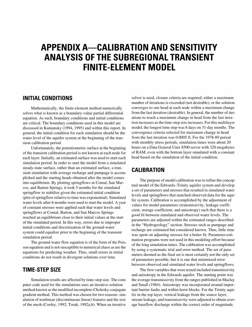
APPENDIX A—CALIBRATION AND SENSITIVITY ANALYSIS OF THE SUBREGIONAL TRANSIENT
FINITE-ELEMENT MODEL
INITIAL CONDITIONS
Mathematically, the finite-element method numerically solves what is known as a boundary-value partial differential equation. As such, boundary conditions and initial conditions are critical. The boundary conditions used in this model are discussed in Kuniansky (1994, 1995) and within this report. In general, the initial condition for each simulation should be the water level of the aquifer system at the beginning of the tran-sient calibration period.
Unfortunately, the potentiometric surface at the beginning of the transient calibration period is not known at each node for each layer. Initially, an estimated surface was used to start each simulation period. In order to start the model from a simulated steady-state surface, rather than an estimated surface, a tran-sient simulation with average recharge and pumpage is accom-plished and the starting heads obtained after the model comes into equilibrium. By plotting springflows at Comal, San Mar-cos, and Barton Springs, it took 5 months for the simulated springflow to stabilize given the estimated initial condition (plot of springflow relative to time was exponential). Simulated water levels after 6 months were used to start the model. A year of constant stresses were applied such that water levels and springflows at Comal, Barton, and San Marcos Springs reached an equilibrium close to their initial values at the start of the simulated period. In this way, errors due to improper initial conditions and discretization of the ground-water system could equalize prior to the beginning of the transient simulation period.
The ground-water flow equation is of the form of the Pois-son equation and is not susceptible to numerical chaos as are the equations for predicting weather. Thus, small errors in initial conditions do not result in divergent solutions over time.
TIME-STEP SIZE
Simulation results are affected by time-step size. The com-puter code used for the simulations uses an iterative-solution method known as the modified incomplete-Cholesky conjugate gradient method. This method was chosen for two reasons: sim-ulation of nonlinear (discontinuous linear) features and the size of the mesh (Cooley, 1992; Torak, 1992a,b). When an iterative
solver is used, closure criteria are required; either a maximum number of iterations is exceeded (not desirable), or the solution converges to one head at each node within a maximum change from the last iteration (desirable). In general, the number of iter-ations to reach a maximum change in head from the last itera-tion increases as the time-step size increases. For this multilayer model, the longest time step was 6 days on 31-day months. The convergence criteria selected for maximum change in head from the last iteration was 0.0005 ft. For the 1978-89 period with monthly stress periods, simulation times were about 20 hours on a Data General Unix 8500 server with 320 megabytes of RAM, even with the bottom layer simulated with a constant head based on the simulation of the initial condition.
CALIBRATION
The purpose of model calibration was to refine the concep-tual model of the Edwards–Trinity aquifer system and develop a set of parameters and stresses that resulted in simulated water levels and springflows that matched observed data for the aqui-fer system. Calibration is accomplished by the adjustment of values for model parameters (transmissivity, leakage coeffi-cient, storage coefficient, and anisotropy) such that there is a good fit between simulated and observed water levels. The parameters are adjusted within the estimated ranges described in the “Hydrogeology” section. Stresses such as pumpage and recharge are estimated but considered known. Thus, little time was spent on adjusting stresses for a better fit. Parameter-esti-mation programs were not used in this modeling effort because of the long simulation times. The calibration was accomplished by using a systematic trial and error method. The set of para-meters deemed as the final set is most certainly not the only set of parameters possible, but it is one that minimized error between observed and simulated water levels and springflows.
The first variables that were tested included transmissivity and anisotropy in the Edwards aquifer. The starting point was the average transmissivity from the ranges published in Maclay and Small (1984). Anisotropy was incorporated around impor-tant barrier faults and within horst blocks. For the Trinity aqui-fer in the top layer, vertical leakage from the source layer, stream leakage, and transmissivity were adjusted to obtain aver-age baseflow discharge within the correct order of magnitude.
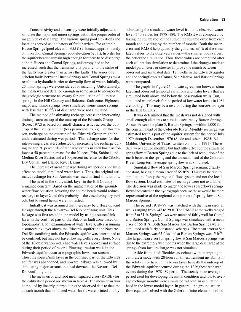
Calibration 73
Transmissivity and anisotropy were initially adjusted to simulate the major and minor springs within the proper order of magnitude of discharge. The various spring pool elevations and locations served as indicators of fault barriers. For example, Hueco Springs (pool elevation 655 ft) is located approximately 3 mi north of Comal Springs (pool elevation 623 ft). In order for the aquifer head to remain high enough for there to be discharge at both Hueco and Comal Springs, anisotropy had to be increased, such that the transmissivity parallel to the strike of the faults was greater than across the faults. The series of en echelon faults between Hueco Springs and Comal Springs must result in a hydraulic barrier to downdip flow of water. Initially, 25 minor springs were considered for matching. Unfortunately, the mesh was not detailed enough in some areas to incorporate the geologic structure necessary for simulation of all minor springs in the Hill Country and Balcones fault zone. Eighteen major and minor springs were simulated; some minor springs with less than 10 ft3/s of discharge were not simulated.
The method of estimating recharge across the intervening drainage area on top of the outcrop of the Edwards Group (Rose, 1972) is based on runoff characteristics across the out-crop of the Trinity aquifer (less permeable rocks). For this rea-son, recharge on the outcrop of the Edwards Group might be underestimated during wet periods. The recharge rates for the intervening areas were adjusted by increasing the recharge dur-ing the top 30 percentile of recharge events in each basin as fol-lows; a 50 percent increase for the Nueces, Frio, Sabinal, and Medina River Basins and a 100 percent increase for the Cibolo, Dry Comal, and Blanco River Basins.
The increase of areal recharge during wet periods had little effect on model-simulated water levels. Thus, the original esti-mated recharge for San Antonio was used in final simulations.
The head in the source/sink layer in the Hill Country remained constant. Based on the mathematics of the ground-water flow equation, lowering the source heads would reduce recharge to layer 2 and this probably is the case during dry peri-ods, but lowered heads were not tested.
Initially, it was assumed that there may be diffuse upward leakage through the Navarro–Del Rio confining unit. This leakage was first tested in the model by using a source/sink layer in the confined part of the Balcones fault zone based on topography. Upon examination of water levels, after assuming a source/sink layer above the Edwards aquifer in the Navarro–Del Rio confining unit, the Edwards aquifer was determined to be confined, but may not have flowing wells everywhere. None of the 10 observation wells had water levels above land surface during their period of record. Flowing artesian wells in the Edwards aquifer occur at topographic lows near streams. Thus, the source/sink layer in the confined part of the Edwards aquifer was abandoned, and upward leakage was allowed by simulating major streams that had downcut the Navarro–Del Rio confining unit.
The mean error and root mean squared error (RMSE) for the calibration period are shown in table 4. The mean error was computed by linearly interpolating the observed data to the time at each month that simulated water levels were printed and by
subtracting the simulated water level from the observed water level (143 values for 1978–89). The RMSE was computed by taking the square root of the sum of the squared error from each month and dividing by the number of months. Both the mean error and RMSE help quantify the goodness of fit of the simu-lated values to the observed values—the smaller both values, the better the simulation. Thus, these values are computed after each calibration simulation to determine if the changes made to model parameters or stresses improve the match between observed and simulated data. Ten wells in the Edwards aquifer and the springflows at Comal, San Marcos, and Barton Springs were compared.
The graphs in figure 25 indicate agreement between simu-lated and observed temporal variations and water levels that are simulated both above and below the observation wells. But, simulated water levels for the period of low water levels in 1984 are too high. This may be a result of using the source/sink layer in the Hill Country.
It was determined that the mesh was not designed with small enough elements to simulate accurately Barton Springs. As can be seen on plate 3, Barton Springs is within 1,000 ft of the constant head of the Colorado River. Monthly recharge was estimated for this part of the aquifer system for the period July 1979 through December 1976 (Slade and others, 1985; B.J. Mahler, University of Texas, written commun., 1991). These data were applied monthly but had little effect on the simulated springflow at Barton Springs due to the lack of resolution of the mesh between the spring and the constant head of the Colorado River. Long-term average springflow was simulated.
Simulated flow of San Marcos Springs remained fairly constant, having a mean error of 65 ft3/s. This may be due to simulation of only the regional flow system and not the local flow system. Local estimates of recharge were not available. The decision was made to match the lower (baseflow) spring-flows indicated on the hydrograph because these would be more representative of the regional component of springflow at San Marcos Springs.
The period 1978–89 was matched with the mean error at wells ranging from -47 to 29 ft. The RMSE at the wells ranged from 2 to 51 ft. Springflows were matched fairly well for Comal and Barton Springs. Comal Springs was simulated with a mean error of 65 ft3/s. Both San Marcos and Barton Springs were simulated with fairly constant discharges. The mean error at San Marcos Springs was 65 ft3/s and at Barton Springs was -5 ft3/s. The large mean error for springflow at San Marcos Springs was due to the extremely wet months when the large discharge at the springs from local recharge was not simulated.
Aside from the difficulties associated with attempting to calibrate a model with 20-hour run times, transient instability in the solution for head in the lower layer beneath the outcrop of the Edwards aquifer occurred during the 12 highest recharge events during the 1978–89 period. The steady-state average period used for developing the initial condition and low to aver-age recharge months were simulated without an oscillation in head in the lower model layer. In general, the ground-water flow equation solved with the Galerkin finite-element method
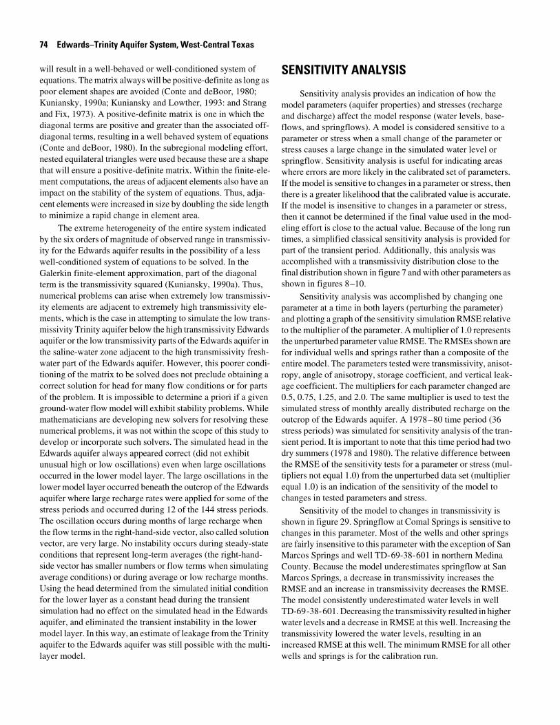
74 Edwards–Trinity Aquifer System, West-Central Texas
will result in a well-behaved or well-conditioned system of equations. The matrix always will be positive-definite as long as poor element shapes are avoided (Conte and deBoor, 1980; Kuniansky, 1990a; Kuniansky and Lowther, 1993: and Strang and Fix, 1973). A positive-definite matrix is one in which the diagonal terms are positive and greater than the associated off-diagonal terms, resulting in a well behaved system of equations (Conte and deBoor, 1980). In the subregional modeling effort, nested equilateral triangles were used because these are a shape that will ensure a positive-definite matrix. Within the finite-ele-ment computations, the areas of adjacent elements also have an impact on the stability of the system of equations. Thus, adja-cent elements were increased in size by doubling the side length to minimize a rapid change in element area.
The extreme heterogeneity of the entire system indicated by the six orders of magnitude of observed range in transmissiv-ity for the Edwards aquifer results in the possibility of a less well-conditioned system of equations to be solved. In the Galerkin finite-element approximation, part of the diagonal term is the transmissivity squared (Kuniansky, 1990a). Thus, numerical problems can arise when extremely low transmissiv-ity elements are adjacent to extremely high transmissivity ele-ments, which is the case in attempting to simulate the low trans-missivity Trinity aquifer below the high transmissivity Edwards aquifer or the low transmissivity parts of the Edwards aquifer in the saline-water zone adjacent to the high transmissivity fresh-water part of the Edwards aquifer. However, this poorer condi-tioning of the matrix to be solved does not preclude obtaining a correct solution for head for many flow conditions or for parts of the problem. It is impossible to determine a priori if a given ground-water flow model will exhibit stability problems. While mathematicians are developing new solvers for resolving these numerical problems, it was not within the scope of this study to develop or incorporate such solvers. The simulated head in the Edwards aquifer always appeared correct (did not exhibit unusual high or low oscillations) even when large oscillations occurred in the lower model layer. The large oscillations in the lower model layer occurred beneath the outcrop of the Edwards aquifer where large recharge rates were applied for some of the stress periods and occurred during 12 of the 144 stress periods. The oscillation occurs during months of large recharge when the flow terms in the right-hand-side vector, also called solution vector, are very large. No instability occurs during steady-state conditions that represent long-term averages (the right-hand-side vector has smaller numbers or flow terms when simulating average conditions) or during average or low recharge months. Using the head determined from the simulated initial condition for the lower layer as a constant head during the transient simulation had no effect on the simulated head in the Edwards aquifer, and eliminated the transient instability in the lower model layer. In this way, an estimate of leakage from the Trinity aquifer to the Edwards aquifer was still possible with the multi-layer model.
SENSITIVITY ANALYSIS
Sensitivity analysis provides an indication of how the model parameters (aquifer properties) and stresses (recharge and discharge) affect the model response (water levels, base-flows, and springflows). A model is considered sensitive to a parameter or stress when a small change of the parameter or stress causes a large change in the simulated water level or springflow. Sensitivity analysis is useful for indicating areas where errors are more likely in the calibrated set of parameters. If the model is sensitive to changes in a parameter or stress, then there is a greater likelihood that the calibrated value is accurate. If the model is insensitive to changes in a parameter or stress, then it cannot be determined if the final value used in the mod-eling effort is close to the actual value. Because of the long run times, a simplified classical sensitivity analysis is provided for part of the transient period. Additionally, this analysis was accomplished with a transmissivity distribution close to the final distribution shown in figure 7 and with other parameters as shown in figures 8–10.
Sensitivity analysis was accomplished by changing one parameter at a time in both layers (perturbing the parameter) and plotting a graph of the sensitivity simulation RMSE relative to the multiplier of the parameter. A multiplier of 1.0 represents the unperturbed parameter value RMSE. The RMSEs shown are for individual wells and springs rather than a composite of the entire model. The parameters tested were transmissivity, anisot-ropy, angle of anisotropy, storage coefficient, and vertical leak-age coefficient. The multipliers for each parameter changed are 0.5, 0.75, 1.25, and 2.0. The same multiplier is used to test the simulated stress of monthly areally distributed recharge on the outcrop of the Edwards aquifer. A 1978–80 time period (36 stress periods) was simulated for sensitivity analysis of the tran-sient period. It is important to note that this time period had two dry summers (1978 and 1980). The relative difference between the RMSE of the sensitivity tests for a parameter or stress (mul-tipliers not equal 1.0) from the unperturbed data set (multiplier equal 1.0) is an indication of the sensitivity of the model to changes in tested parameters and stress.
Sensitivity of the model to changes in transmissivity is shown in figure 29. Springflow at Comal Springs is sensitive to changes in this parameter. Most of the wells and other springs are fairly insensitive to this parameter with the exception of San Marcos Springs and well TD-69-38-601 in northern Medina County. Because the model underestimates springflow at San Marcos Springs, a decrease in transmissivity increases the RMSE and an increase in transmissivity decreases the RMSE. The model consistently underestimated water levels in well TD-69-38-601. Decreasing the transmissivity resulted in higher water levels and a decrease in RMSE at this well. Increasing the transmissivity lowered the water levels, resulting in an increased RMSE at this well. The minimum RMSE for all other wells and springs is for the calibration run.
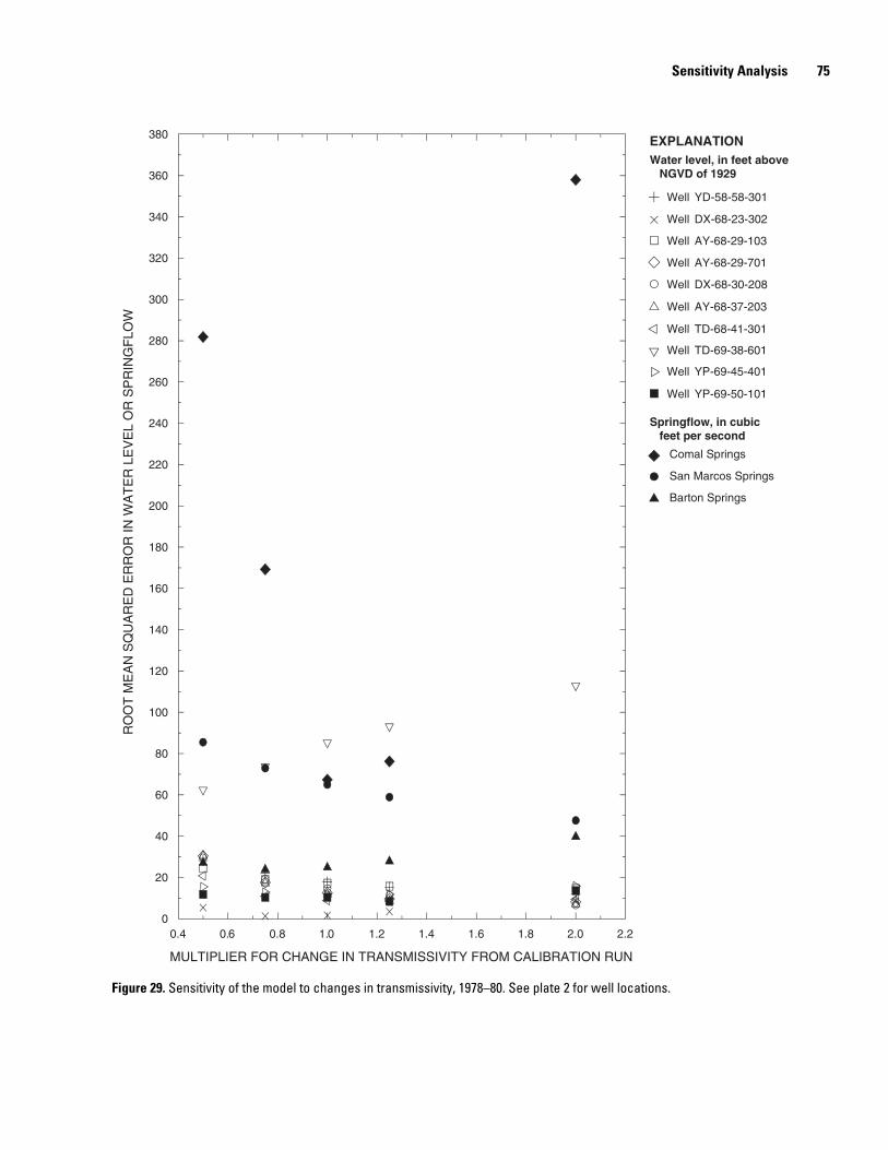
Sensitivity Analysis 75
Figure 29. Sensitivity of the model to changes in transmissivity, 1978–80. See plate 2 for well locations.
0
380
20
40
60
80
100
120
140
160
180
200
220
240
260
280
300
320
340
360
RO
OT
ME
AN
SQ
UA
RE
D E
RR
OR
IN W
AT
ER
LE
VE
L O
R S
PR
ING
FLO
W
0.4 2.20.6 0.8 1.0 1.2 1.4 1.6 1.8 2.0
MULTIPLIER FOR CHANGE IN TRANSMISSIVITY FROM CALIBRATION RUN
YD-58-58-301
DX-68-23-302
AY-68-29-103
AY-68-29-701
DX-68-30-208
AY-68-37-203
TD-68-41-301
TD-69-38-601
YP-69-45-401
YP-69-50-101
Comal Springs
San Marcos Springs
Barton Springs
Water level, in feet above NGVD of 1929
Springflow, in cubic feet per second
EXPLANATION
Well
Well
Well
Well
Well
Well
Well
Well
Well
Well
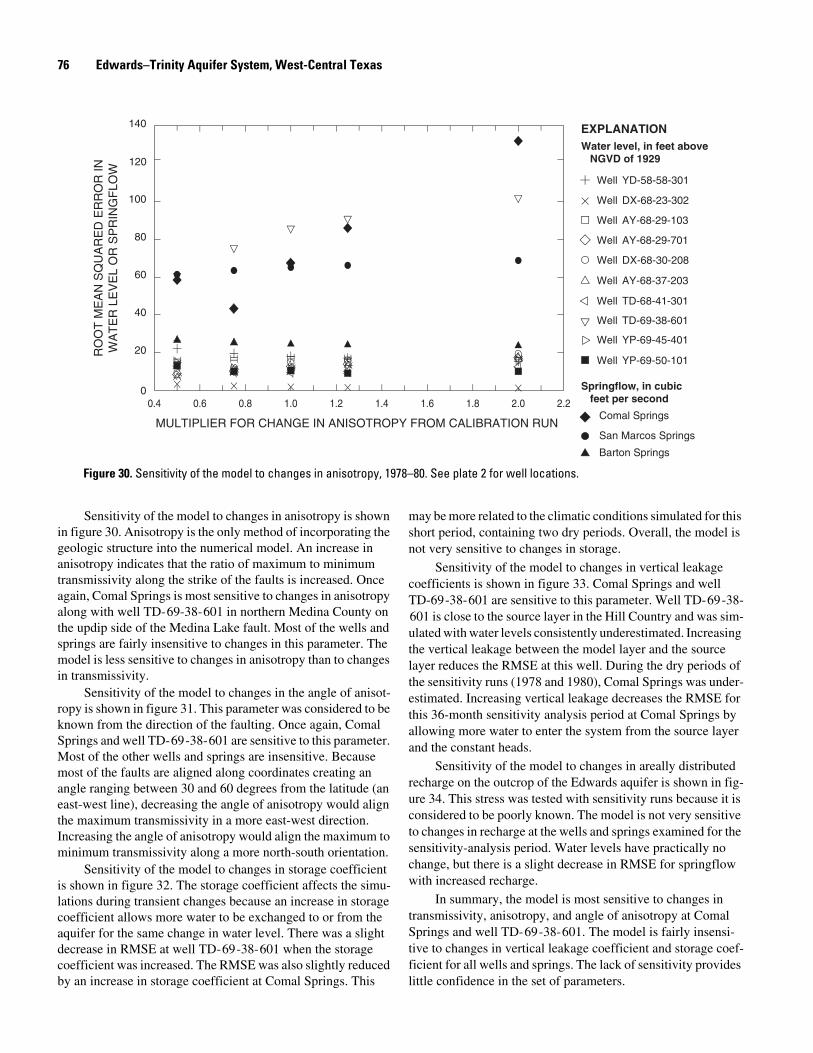
76 Edwards–Trinity Aquifer System, West-Central Texas
Figure 30. Sensitivity of the model to changes in anisotropy, 1978–80. See plate 2 for well locations.
0
140
20
40
60
80
100
0.4 0.6 0.8 1.0 1.2 1.4 1.6 1.8 2. 2.20
RO
OT
ME
AN
SQ
UA
RE
D E
RR
OR
INW
AT
ER
LE
VE
L O
R S
PR
ING
FLO
W
120
MULTIPLIER FOR CHANGE IN ANISOTROPY FROM CALIBRATION RUN
YD-58-58-301
DX-68-23-302
AY-68-29-103
AY-68-29-701
DX-68-30-208
AY-68-37-203
TD-68-41-301
TD-69-38-601
YP-69-45-401
YP-69-50-101
Comal Springs
San Marcos Springs
Barton Springs
Water level, in feet above NGVD of 1929
Springflow, in cubic feet per second
EXPLANATION
Well
Well
Well
Well
Well
Well
Well
Well
Well
Well
Sensitivity of the model to changes in anisotropy is shown in figure 30. Anisotropy is the only method of incorporating the geologic structure into the numerical model. An increase in anisotropy indicates that the ratio of maximum to minimum transmissivity along the strike of the faults is increased. Once again, Comal Springs is most sensitive to changes in anisotropy along with well TD-69-38-601 in northern Medina County on the updip side of the Medina Lake fault. Most of the wells and springs are fairly insensitive to changes in this parameter. The model is less sensitive to changes in anisotropy than to changes in transmissivity.
Sensitivity of the model to changes in the angle of anisot-ropy is shown in figure 31. This parameter was considered to be known from the direction of the faulting. Once again, Comal Springs and well TD-69-38-601 are sensitive to this parameter. Most of the other wells and springs are insensitive. Because most of the faults are aligned along coordinates creating an angle ranging between 30 and 60 degrees from the latitude (an east-west line), decreasing the angle of anisotropy would align the maximum transmissivity in a more east-west direction. Increasing the angle of anisotropy would align the maximum to minimum transmissivity along a more north-south orientation.
Sensitivity of the model to changes in storage coefficient is shown in figure 32. The storage coefficient affects the simu-lations during transient changes because an increase in storage coefficient allows more water to be exchanged to or from the aquifer for the same change in water level. There was a slight decrease in RMSE at well TD-69-38-601 when the storage coefficient was increased. The RMSE was also slightly reduced by an increase in storage coefficient at Comal Springs. This
may be more related to the climatic conditions simulated for this short period, containing two dry periods. Overall, the model is not very sensitive to changes in storage.
Sensitivity of the model to changes in vertical leakage coefficients is shown in figure 33. Comal Springs and well TD-69-38-601 are sensitive to this parameter. Well TD-69-38-601 is close to the source layer in the Hill Country and was sim-ulated with water levels consistently underestimated. Increasing the vertical leakage between the model layer and the source layer reduces the RMSE at this well. During the dry periods of the sensitivity runs (1978 and 1980), Comal Springs was under-estimated. Increasing vertical leakage decreases the RMSE for this 36-month sensitivity analysis period at Comal Springs by allowing more water to enter the system from the source layer and the constant heads.
Sensitivity of the model to changes in areally distributed recharge on the outcrop of the Edwards aquifer is shown in fig-ure 34. This stress was tested with sensitivity runs because it is considered to be poorly known. The model is not very sensitive to changes in recharge at the wells and springs examined for the sensitivity-analysis period. Water levels have practically no change, but there is a slight decrease in RMSE for springflow with increased recharge.
In summary, the model is most sensitive to changes in transmissivity, anisotropy, and angle of anisotropy at Comal Springs and well TD-69-38-601. The model is fairly insensi-tive to changes in vertical leakage coefficient and storage coef-ficient for all wells and springs. The lack of sensitivity provides little confidence in the set of parameters.
Sensitivity Analysis 77
Figure 31. Sensitivity of the model to changes in angle of anisotropy, 1978–80. See plate 2 for well locations.
0
220
20
40
60
80
100
120
140
160
180
200
0.4 2.20.6 0.8 1.0 1.2 1.4 1.6 1.8 2.0
MULTIPLIER FOR CHANGE IN ANGLE OF ANISOTROPY FROM CALIBRATION RUN
RO
OT
ME
AN
SQ
UA
RE
D E
RR
OR
IN W
AT
ER
LE
VE
L O
R S
PR
ING
FLO
W
YD-58-58-301
DX-68-23-302
AY-68-29-103
AY-68-29-701
DX-68-30-208
AY-68-37-203
TD-68-41-301
TD-69-38-601
YP-69-45-401
YP-69-50-101
Comal Springs
San Marcos Springs
Barton Springs
Water level, in feet above NGVD of 1929
Springflow, in cubic feet per second
EXPLANATION
Well
Well
Well
Well
Well
Well
Well
Well
Well
Well
Figure 32. Sensitivity of the model to changes in storage coefficient, 1978–80. See plate 2 for well locations.
0
100
10
20
30
40
50
60
70
80
90
0.4 2.20.6 0.8 1.0 1.2 1.4 1.6 1.8 2.0
MULTIPLIER FOR CHANGE IN VERTICAL LEAKAGE COEFFICIENT FROM CALIBRATION RUN
RO
OT
ME
AN
SQ
UA
RE
D E
RR
OR
INW
AT
ER
LE
VE
L O
R S
PR
ING
FLO
W
YD-58-58-301
DX-68-23-302
AY-68-29-103
AY-68-29-701
DX-68-30-208
AY-68-37-203
TD-68-41-301
TD-69-38-601
YP-69-45-401
YP-69-50-101
Comal Springs
San Marcos Springs
Barton Springs
Water level, in feet above NGVD of 1929
Springflow, in cubic feet per second
EXPLANATION
Well
Well
Well
Well
Well
Well
Well
Well
Well
Well
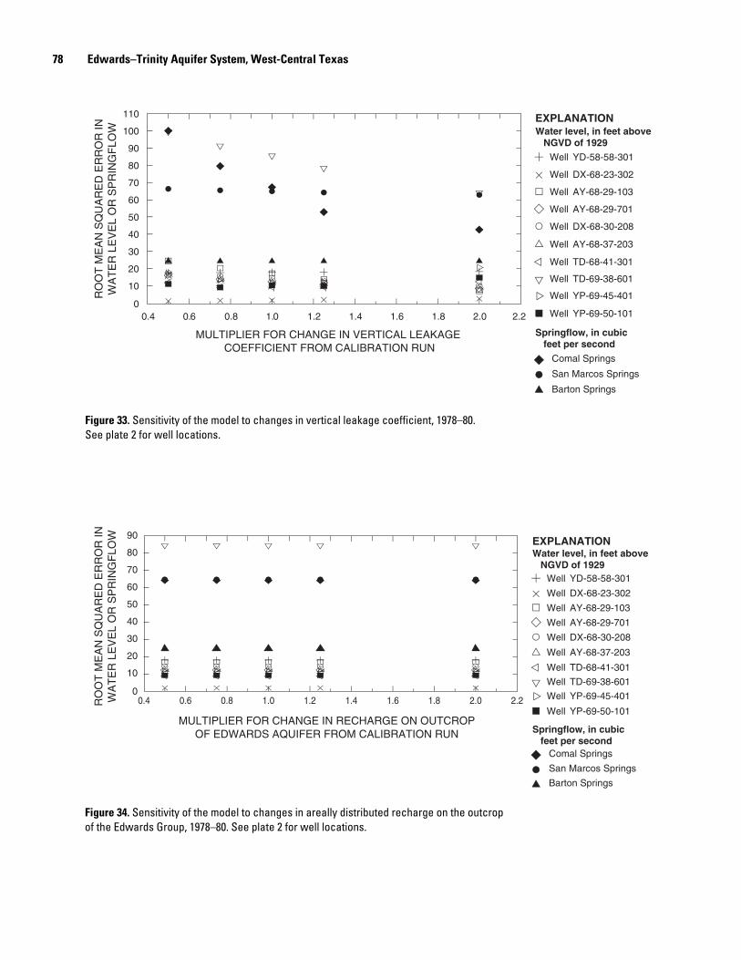
78 Edwards–Trinity Aquifer System, West-Central Texas
Figure 33. Sensitivity of the model to changes in vertical leakage coefficient, 1978–80. See plate 2 for well locations.
0
110
10
20
30
40
50
60
70
80
90
100
0.4 2.20.6 0.8 1.0 1.2 1.4 1.6 1.8 2.0
MULTIPLIER FOR CHANGE IN VERTICAL LEAKAGE COEFFICIENT FROM CALIBRATION RUN
RO
OT
ME
AN
SQ
UA
RE
D E
RR
OR
INW
AT
ER
LE
VE
L O
R S
PR
ING
FLO
W
YD-58-58-301
DX-68-23-302
AY-68-29-103
AY-68-29-701
DX-68-30-208
AY-68-37-203
TD-68-41-301
TD-69-38-601
YP-69-45-401
YP-69-50-101
Comal Springs
San Marcos Springs
Barton Springs
Water level, in feet above NGVD of 1929
Springflow, in cubic feet per second
EXPLANATION
Well
Well
Well
Well
Well
Well
Well
Well
Well
Well
Figure 34. Sensitivity of the model to changes in areally distributed recharge on the outcrop of the Edwards Group, 1978–80. See plate 2 for well locations.
0
90
10
20
30
40
50
60
70
80
0.4 2.20.6 0.8 1.0 1.2 1.4 1.6 1.8 2.0RO
OT
ME
AN
SQ
UA
RE
D E
RR
OR
INW
AT
ER
LE
VE
L O
R S
PR
ING
FLO
W
MULTIPLIER FOR CHANGE IN RECHARGE ON OUTCROPOF EDWARDS AQUIFER FROM CALIBRATION RUN
YD-58-58-301
DX-68-23-302
AY-68-29-103
AY-68-29-701
DX-68-30-208
AY-68-37-203
TD-68-41-301
TD-69-38-601
YP-69-45-401
YP-69-50-101
Comal Springs
San Marcos Springs
Barton Springs
Water level, in feet above NGVD of 1929
Springflow, in cubic feet per second
EXPLANATION
Well
Well
Well
Well
Well
Well
Well
Well
Well
Well


![[PPT]Vulernability map of the Edwards Aquifer - University of … · Web viewVulnerability map of the Edwards Aquifer Aquifer DRASTIC INDEX 84 - 90 90 - 978 97 - 104 104 – 111 111](https://static.fdocuments.in/doc/165x107/5aebf7d37f8b9ab24d8f7734/pptvulernability-map-of-the-edwards-aquifer-university-of-viewvulnerability.jpg)