The Edwards Aquifer Recovery and Implementation Program
159
Technical Assessments in Support of the Edwards Aquifer Science Committee “J Charge” Flow Regime Evaluation for the Comal and San Marcos River Systems Prepared for: The Edwards Aquifer Recovery and Implementation Program Prepared by: Dr. Thomas B. Hardy, Ph.D. River Systems Institute Texas State University San Marcos, Texas December 29, 2009
Transcript of The Edwards Aquifer Recovery and Implementation Program

Technical Assessments in Support of the Edwards Aquifer Science Committee “J
Charge” Flow Regime Evaluation for the Comal and San Marcos River Systems
Prepared for:
The Edwards Aquifer Recovery and Implementation Program
Prepared by:
Dr. Thomas B. Hardy, Ph.D.
River Systems Institute
Texas State University
San Marcos, Texas
December 29, 2009

Acknowledgments
Many individuals from private, local, state, and federal agencies contributed to the development of
material summarized in this report. Without their input and efforts, this report would not have been
possible. Although the list of individual who in some manner contributed to the data, modeling results,
or scientific material used in this report is extensive and too long to list, the following individuals are
acknowledged as having made significant contributions in terms of both their time and expertise. The
author apologizes for inclusion of anyone who does not wish to be acknowledged or to anyone whom I
have failed to properly acknowledge.
Dr. Mara Alexander
Mr. William Amy
Mr. Karim Aziz
Ms. Megan Bean
Dr. Timothy Bonner
Dr. Tom Brandt
Ms. Jean Cochrane
Mr. Pat Conner
Ms. Melani Howard
Mr. Praveen Kokkanti
Mr. Brad Littrell
Mr. Miguel Mora
Mr. Ed Orborny
Mr. Nathan Pence
Ms. Jackie Poole
Mr. Kenny Saunders
Ms. Jenna Winters
Mr. Adam Zerringer

Table of Contents
Acknowledgments ..................................................................................................................................... ii
Executive Summary ................................................................................................................................... x
Introduction ................................................................................................................................................ 1
Study Areas ................................................................................................................................................ 1
Comal .................................................................................................................................................... 1
San Marcos ............................................................................................................................................ 3
Influence Diagrams for Target Species ...................................................................................................... 4
Comal Springs Riffle Beetle .................................................................................................................. 5
Texas Wild Rice ..................................................................................................................................... 9
Fountain Darters .................................................................................................................................. 10
Hydrodynamic Modeling ......................................................................................................................... 13
Physical Characterization .................................................................................................................... 13
Development of Computational Meshes ............................................................................................. 14
Two-dimensional Hydraulic Models ................................................................................................... 15
Water Surface Elevation Modeling ................................................................................................. 16
Comal River .................................................................................................................................... 17
San Marcos River ........................................................................................................................... 20
San Marcos No Cape's Dam Alternative Modeling Scenario .................................................... 22
Vegetation Mapping ............................................................................................................................ 22
Vegetation Dependent Hydraulic Roughness ...................................................................................... 23
Vertical Velocity Distributions in Vegetation ...................................................................................... 25
Water Quality and Temperature Modeling ............................................................................................... 25
Comal River ........................................................................................................................................ 25
Boundary Conditions ...................................................................................................................... 28
Model Calibration and Verification ................................................................................................ 30
San Marcos River ................................................................................................................................ 31
Boundary Conditions ...................................................................................................................... 31
Model Calibration and Verification ................................................................................................ 34
Habitat Suitability Curves ........................................................................................................................ 35
Comal Springs Riffle Beetle ................................................................................................................ 36
Texas Wild Rice ................................................................................................................................... 37
Fountain Darters .................................................................................................................................. 40
Physical Habitat Modeling ....................................................................................................................... 44
Comal Springs Riffle Beetle Habitat Equation ................................................................................... 45
Texas Wild Rice Habitat Equation ...................................................................................................... 45
Fountain Darter Habitat Equation ....................................................................................................... 45
Modeling Results and Discussion ............................................................................................................ 45
Comal .................................................................................................................................................. 46
Temperature .................................................................................................................................... 46
Dissolved Oxygen........................................................................................................................... 48
Comal Springs Riffle Beetle ........................................................................................................... 50
Fountain Darter ............................................................................................................................... 52
System-Wide Physical Habitat Using Mean Daily Temperatures ............................................. 52
Physical Habitat Using Maximum Daily Temperatures ............................................................ 54

San Marcos .......................................................................................................................................... 60
Temperature .................................................................................................................................... 60
Dissolved Oxygen........................................................................................................................... 62
Texas Wild Rice .............................................................................................................................. 62
System-Wide Physical Habitat ................................................................................................... 62
Spring Lake ................................................................................................................................ 63
Rio Vista ..................................................................................................................................... 63
Above Cape’s ............................................................................................................................. 64
Mill Race .................................................................................................................................... 64
State Hatchery A ........................................................................................................................ 64
State Hatchery B ........................................................................................................................ 64
Lower San Marcos A ................................................................................................................. 64
Lower San Marcos B ................................................................................................................. 65
Revised Upper San Marcos Physical Habitat Modeling ................................................................ 65
Texas Wild Rice Physical Habitat Summary ............................................................................. 70
Fountain Darter ............................................................................................................................... 74
System-Wide Physical Habitat ................................................................................................... 74
Spring Lake ................................................................................................................................ 74
Rio Vista ..................................................................................................................................... 75
Above Cape’s ............................................................................................................................. 75
Mill Race .................................................................................................................................... 75
State Hatchery A ........................................................................................................................ 75
State Hatchery B ........................................................................................................................ 76
Lower San Marcos A ................................................................................................................. 76
Lower San Marcos B ................................................................................................................. 76
Upper San Marcos Physical Habitat .......................................................................................... 76
Sensitivity to Channel Change and Habitat Suitability Criteria ................................................ 82
Fountain Darter Physical Habitat Summary .............................................................................. 83
Other Native Aquatic Species .................................................................................................................. 83
Comal Springs dryopid beetle (Stygoparnus comalensis) ................................................................... 83
Peck’s cave amphipod (Stygobromus pecki) ....................................................................................... 83
San Marcos Gambusia (Gambusia georgei) ........................................................................................ 83
Texas blind salamanders (Eurycea rathbuni) ....................................................................................... 84
San Marcos salamanders (Eurycea nana) ............................................................................................ 84
Cagle’s map turtle (Graptemys caglei) ................................................................................................ 84
Non-native Species .................................................................................................................................. 84
Suckermouth Catfish (Hypostomus sp.) .............................................................................................. 85
Tilapia (Tilapia sp.) ............................................................................................................................. 86
Nutria (Myocastor coypus) .................................................................................................................. 86
Elephant Ears (Colocasia esculenta) ................................................................................................... 87
Giant Ramshorn Snails (Marisa cornuarietis) ..................................................................................... 87
Asian snail (Melanoides tuberculata) .................................................................................................. 87
Gill Parasite (Centrocestus formosanus) ............................................................................................. 87
Recreation ................................................................................................................................................ 88
Summary .................................................................................................................................................. 88
Future Study Recommendations .............................................................................................................. 89
References Cited ...................................................................................................................................... 90

Appendix A .............................................................................................................................................. 93
Definition of terms used in preliminary Edwards Aquifer influence diagrams .................................. 93
Definition of terms not used in preliminary Edwards Aquifer influence diagrams ............................ 98
Submitted revisions and comments to the preliminary Edwards Aquifer influence diagrams ........... 99
Appendix B ............................................................................................................................................ 113
Depth, Velocity, and Combined Suitability Contours for the Fountain Darter in the Comal River for
Simulated Discharges ........................................................................................................................ 113
Appendix C ............................................................................................................................................ 114
Appendix D ............................................................................................................................................ 119
Depth, Velocity, and Combined Suitability Contours for Texas Wild Rice and Fountain Darter in the
San Marcos River for Simulated Discharges .................................................................................... 119
Appendix E ............................................................................................................................................ 120
Comment response matrix for Draft Report ...................................................................................... 120
vi
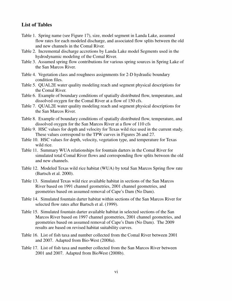
List of Tables
Table 1. Spring name (see Figure 17), size, model segment in Landa Lake, assumed
flow rates for each modeled discharge, and associated flow splits between the old
and new channels in the Comal River.
Table 2. Incremental discharge accretions by Landa Lake model Segments used in the
hydrodynamic modeling of the Comal River.
Table 3. Assumed spring flow contributions for various spring sources in Spring Lake of
the San Marcos River.
Table 4. Vegetation class and roughness assignments for 2-D hydraulic boundary
condition files.
Table 5. QUAL2E water quality modeling reach and segment physical descriptions for
the Comal River.
Table 6. Example of boundary conditions of spatially distributed flow, temperature, and
dissolved oxygen for the Comal River at a flow of 150 cfs.
Table 7. QUAL2E water quality modeling reach and segment physical descriptions for
the San Marcos River.
Table 8. Example of boundary conditions of spatially distributed flow, temperature, and
dissolved oxygen for the San Marcos River at a flow of 110 cfs
Table 9. HSC values for depth and velocity for Texas wild rice used in the current study.
These values correspond to the TPW curves in Figures 26 and 27.
Table 10. HSC values for depth, velocity, vegetation type, and temperature for Texas
wild rice.
Table 11. Summary WUA relationships for fountain darters in the Comal River for
simulated total Comal River flows and corresponding flow splits between the old
and new channels.
Table 12. Modeled Texas wild rice habitat (WUA) by total San Marcos Spring flow rate
(Bartsch et al. 2000).
Table 13. Simulated Texas wild rice available habitat in sections of the San Marcos
River based on 1991 channel geometries, 2001 channel geometries, and
geometries based on assumed removal of Cape’s Dam (No Dam).
Table 14. Simulated fountain darter habitat within sections of the San Marcos River for
selected flow rates after Bartsch et al. (1999).
Table 15. Simulated fountain darter available habitat in selected sections of the San
Marcos River based on 1997 channel geometries, 2001 channel geometries, and
geometries based on assumed removal of Cape’s Dam (No Dam). The 2009
results are based on revised habitat suitability curves.
Table 16. List of fish taxa and number collected from the Comal River between 2001
and 2007. Adapted from Bio-West (2008a).
Table 17. List of fish taxa and number collected from the San Marcos River between
2001 and 2007. Adapted from BioWest (2008b).

vii
List of Figures
Figure 1. Comal River study area. (This figure is being updated to the style in Figure 2)
Figure 2. San Marcos study area.
Figure 3. Key to influence diagram designs.
Figure 4. Comal Springs riffle beetle overall influence diagram.
Figure 5. Habitat factors specific to water quantity for the Comal Springs riffle beetle.
Figure 6. Example of potential human influences on water quantity and quality for the
Comal Springs riffle beetle.
Figure 7. Example of potential human influences on fine sediment input for the Comal
Springs riffle beetle.
Figure 8. Texas wild rice overall influence diagram.
Figure 9. Habitat factors potentially affecting Texas wild rice.
Figure 10. Example of direct mortality factors influence diagram for Texas wild rice.
Figure 11. Fountain darter overall influence diagram.
Figure 12. Habitat factors potentially affecting fountain darters.
Figure 13. Example of direct mortality factors influence diagram for fountain darters.
Figure 14. Example of a three dimensional computational mesh from a section of the San
Marcos River.
Figure 15. Example of 1-dimensional cross sections extracted from the three-dimensional
computational mesh for a section of the Comal River.
Figure 16. Hydrodynamic computational sections for the Comal River system used in the
RMA-2 modeling.
Figure 17. Spatial location of spring inflow nodes within Landa Lake of the Comal River
system used in the hydrodynamic modeling.
Figure 18. Location of 18 springs used in the hydrodynamic modeling of Spring Lake in the
San Marcos River.
Figure 19. Stage discharge relationship from HEC-RAS used to calibrate the Above Cape’s
section No Dam scenario.
Figure 20. Example of vegetation mapping polygons from the Comal River.
Figure 21. Computational segments and computational cells for use in water temperature
and dissolved oxygen modeling in the Comal River System.
Figure 22. Water temperature monitoring stations in the Comal River used for model
calibration.
Figure 23. Calibration data for the bottom of the old channel. Run is for 48 hours. (b)
Verification data for the old channel. Run is for 48 hours.
Figure 24. Water quality computational reaches for the San Marcos River with water
temperature monitoring stations indicated by open circles.
Figure 25. Examples of the water temperature model calibration and verification runs for
the San Marcos River at the City Park and confluence with the Blanco River
monitoring stations.
viii
Figure 26. Texas wild rice depth habitat suitability. See text for explanation of curve
legends.
Figure 27. Texas wild rice velocity habitat suitability. See text for explanation of curve
legends.
Figure 28. Fountain darter depth habitat suitability curves (Depth_Old is Bartsch el al.,
(2000) and Depth_New_Revised is derived from the analysis of the EAA monitoring
data).
Figure 29. Fountain darter velocity habitat suitability (Velocity_Old is Bartsch el al., (2000)
and Velocity_New_Revised is derived from the analysis of the EAA monitoring
data).
Figure 30. Fountain darter vegetation type habitat suitability.
Figure 31. Fountain darter temperature habitat suitability.
Figure 32. Simulated longitudinal temperature profile for modeled flow rate scenarios in the
old channel. Flow rates shown represent overall spring flow rates for each scenario
Figure 33. Simulated longitudinal temperature profile for Landa Lake and the new channel
for modeled flow split scenarios. Flow rates shown are total Comal River flow rates.
The letter 'A' marks significant spring locations in upper Landa Lake, the letter 'B'
marks the main spring runs, the letter 'C' marks the new channel, and the letter 'D'
marks the lower Comal River below Clemens Dam.
Figure 34. Dissolved oxygen concentrations plotted against mile upstream from the end of
the old channel.
Figure 35. Dissolved oxygen concentration plotted against mile upstream from the end of
the confluence with the Guadalupe River. See text for legend explanations.
Figure 36. Simulated Comal Springs riffle beetle habitat based on depth and velocity
criteria within spring runs 1, 2, and 3.
Figure 37. Total estimated fountain darter habitat in the Comal River based on physical
habitat using mean daily water temperatures. Note, suitable areas in this context
reflect potential areas below the thermal threshold at which temperatures are
associated with reduced larval survival.
Figure 38. Available fountain darter habitat in the Comal River at a total flow rate of 30 and
60 cfs based on mean daily temperatures. See figure for flow rate splits in the old
and new channel. Unsuitable habitat in this context simply refers to areas at which
potentially reduced larval survival may occur.
Figure 39. Depth and velocity contour plots at 10 and 40 cfs in the Upper Old Channel
section of the Comal River. Color legends are scaled between 0.0 (red) and the
maximum indicated (blue) in 10 increments of the maximum magnitude indicated.
Figure 40. Combined suitability for fountain darter habitat in the Upper Old Channel
section of the Comal River at 10 and 40 cfs. Legend scale is from 0.0 (red) to 1.0
(blue) in 0.1 increments.
Figure 41. Relationships between total Comal River discharge and simulated available
habitat for fountain darters in the old channel.

ix
Figure 42. Relationships between total Comal River discharge and simulated available
habitat for fountain darters in the new channel.
Figure 43. Major simulation reaches utilized by Bartsch et al. (1999).
Figure 44. Relationship between total San Marcos discharge (cfs) and reach level
maximum daily temperatures in selected reaches.
Figure 45. Simulated Texas wild rice available habitat (WUA) in sections of the San
Marcos River based on 1997 channel geometries, 2001 channel geometries, and
geometries based on assumed removal of Cape’s Dam (No Dam). The total area
based on 2001 geometry is also shown as a percent of the maximum habitat.
Figure 46. Spatial distribution of predicted Texas wild rice computational cell suitability
ranges versus the 1989 to 2001 spatial distribution of Texas wild rice stands (red
dots) in the Rio Vista to Cape’s Dam section. Simulated discharge is 65 cfs.
Figure 47. Frequency histograms of simulated cell suitabilities containing Texas wild rice
based at 30 and 65 cfs.
Figure 48. Combined suitability for Texas wild rice habitat in the Spring Lake to Rio Vista
section of the San Marcos River at 15 cfs.
Figure 49. Combined suitability for Texas wild rice habitat in the Spring Lake to Rio Vista
section of the San Marcos River at 30 cfs.
Figure 50. Combined suitability for Texas wild rice habitat in the Spring Lake to Rio Vista
section of the San Marcos River at 65 cfs.
Figure 51. Simulated fountain darter available habitat (WUA) in sections of the San Marcos
River based on 1991 channel geometries, 2001 channel geometries, and geometries
based on assumed removal of Cape’s Dam (No Dam).
Figure 52. Combined suitability for fountain darter habitat in the Spring Lake to Rio Vista
section of the San Marcos River at 15 cfs.
Figure 53. Combined suitability for fountain darter habitat in the Spring Lake to Rio Vista
section of the San Marcos River at 30 cfs.
Figure 54. Combined suitability for fountain darter habitat in the Spring Lake to Rio Vista
section of the San Marcos River at 65 cfs.
Figure 55. Relationship between total San Marcos river discharge and simulated available
fountain darter habitat as a percent of maximum habitat.

x
Executive Summary
This report summarizes the technical analysis of the flow dependent characteristics of physical habitat
for target aquatic species within the Comal and San Marcos Rivers to support the Science Committee
of the Edwards Aquifer Recovery Implementation Program in development of their recommendations
for flow regimes under Senate Bill 2 'J Charges'. Target species were fountain darter (Etheostoma
fonticola), Texas wild rice (Zizania texana), and the Comal Springs riffle beetle (Heterelmis
comalensis). In addition, qualitative assessments of other native and non-native species as well as
recreation were considered.
A team of private, state, federal, and university researchers knowledgeable with the target species and
in particular, the Comal and San Marcos River systems were used to develop influence diagrams for the
three target species to aid the evaluation of both intrinsic and extrinsic factors that affect the persistence
of these target species. The team also used these diagrams to evaluate existing data and specific
modeling approaches to aid in their evaluations of flow regimes for each river system. As part of this
process, the team considered other factors such as non-native species of plants and animals, parasites,
recreation, and anthropogenic impacts due to watershed development.
Historical research and existing physical, chemical, and biological monitoring data collected through
2009 from both the Comal and San Marcos Rivers were integrated to develop biological response
functions for factors such as depth, velocity, substrate/vegetation use, water temperatures, etc. Habitat
suitability curves were reviewed for fountain darters, Texas wild rice, and Comal Springs riffle beetles
based on new data collected over the past eight years. Existing monitoring data were used to update
the fountain darter habitat suitability curves for depth and velocity. No modifications were made to the
Texas wild rice habitat suitability curves and as noted below, simulations of available habitat for the
Comal Springs riffle beetle relied on a simplified surface area analysis as well as an alternative analysis
based on data collected during the original Comal River studies. Vegetation maps relied upon those
derived from the original studies conducted in the Comal and San Marcos due to lack of system-wide
revised vegetation mapping data being available. These existing or revised habitat suitability curves
for the target species, in conjunction with the two-dimensional hydrodynamic models for each river and
associated one-dimensional water quality/temperature models for the Comal and San Marcos Rivers
were used to predict the location and quality of wild rice, fountain darter, and riffle beetle habitat as a
function of different flow ranges in each river system. No new water quality modeling was undertaken
and the report relied upon the previous modeling results for both river systems. Model sensitivity to
changes in channel topographies and habitat suitability curves for depth and velocity for fountain
darters were also explored.
Updated modeling results show that the largest difference in the habitat versus flow relationships for
fountain darters were attributed to differences in habitat suitability curves. Modeling of fountain darter
habitat for pre versus post 1998 flood induced channel changes in the San Marcos River primarily
resulted in a scaling of the magnitude of predicted available habitat rather than a substantive change in
the functional relationship. In both the San Marcos and Comal River systems, potentially adverse
thermal conditions may begin to limit darter larval survival under very low flow conditions.
Modeling results for Texas wild rice in the San Marcos River suggest that habitat availability begins to
xi
decline below about 65 cfs with increasing risk to physical disturbance and drying, especially at and
below 30 cfs. The modeling results also suggest that protection of Texas wild rice would likely ensure
protection for the other target species such as fountain darters.
Modeling results for the Comal Springs riffle beetle based on total surface area in the main spring runs
(i.e, 1,2, and3) were somewhat insensitive to modeled total Comal flow rates as low as 30 cfs.
However, maintaining spring run flows provides the most conservative strategy as it provides the best
overall protection for the other flow dependent aquatic resources such as fountain darters and other
native species.
Based on modeling results and analysis, recommendations are made for future work in light of the on-
going data collection and modeling in support of the Edward Aquifer Habitat Conservation Plan.
Although this report provides the technical documentation on modeling approaches and summary
results, no specific flow recommendations are made. The Science Committee of the Edwards Aquifer
Recovery Implementation Program will recommend target flow regimes for each river system.

1
River Systems Institute
Introduction
The primary modeling approaches adapted for this report were originally reported in Hardy et al (1998)
for the Comal River, and from Bartsch et al. (2000), INSE (2004), and Saunders et al. (2001) for the
San Marcos River. Additional data, analysis, and published research were also relied upon as noted
throughout the report. The work reported here includes both quantitative and qualitative assessments
of flow regimes on the target aquatic species; fountain darters, Texas wild rice, Comal Springs riffle
beetle as well as other flow dependent aquatic resources.
The focus of this report is to provide technical analysis in support to the Expert Science Subcommittee
of the Edwards Aquifer Recovery Implementation Program to evaluate flow regimes for each river
system required under Senate Bill 3 "J" charges. To that end, the original technical work cited above
was reanalyzed using updated biological information to examine the quantity and quality of available
habitat for Texas wild rice, Comal Springs riffle beetle, and fountain darters. These assessments
include a quantitative evaluation of water quality and temperature as well as the qualitative evaluation
of other factors such as recreation, parasites, and non-native species.
To accomplish this effort, a team of knowledgeable scientists with specific experience in the Comal and
San Marcos rivers as well as research on the primary target species were brought together to review the
existing biological data and updated modeling results based on refined habitat suitability information
for the three target species (i.e., Texas wild rice, Comal Riffle beetle, and fountain darter).
Study Areas
Physical, chemical, and biological data were available for each river system from a variety of research
efforts. Collection of physical, chemical, and biological data was undertaken from their respective
spring sources downstream to their confluence with the next river junction as part of the original work
by Hardy et al. (1998) for the Comal River, and by Bartsch et al. (2000), INSE (2004), and Saunders et
al. (2001) for the San Marcos River. Additional biological monitoring data has also been collected as
noted below.
Comal
The Comal River is a 3.2 mile long system located in New Braunfels, Texas (Figure 1). Flow enters
Landa Lake from fissures in the Edwards Aquifer. A prominent feature of the park is the three main
spring runs which contribute between 22.9 to 30 percent of the total spring flow with a median value of
23.8 percent (McKinney et al. 1995; USU measurements, 1998; BioWest 2003 – 2008). The rest of the
water enters the lake via various seeps and spring runs. A fairly constant flow of 30 cfs exits the lake
by the old channel outlets at the golf course tee box and at the spring fed pool while the rest of the flow
exits the bottom of Landa Lake down the new channel. Historically, the old channel bypass was
constrained to approximately 40 cfs before small, low lying areas of the golf course adjacent to the old
channel become inundated. Upgrades to the culvert system can now accommodate up to approximately
100 cfs. The old channel and new channel join just above Clemmen’s Dam and flow another 1.2 miles
downstream to the confluence with the Guadalupe River. An analysis was undertaken to examine the
relationship between flow and the quantity and quality of available habitat for several flow split
scenarios between the old and new channels as noted below.

2
River Systems Institute
Figure 1. Comal River study area.

3
River Systems Institute
San Marcos
The San Marcos River originates from San Marcos Springs in Spring Lake, San Marcos, Hays County,
Texas. The river flows 4.6 miles downstream to a confluence with the Blanco River (Figure 2) and
continues for another 71.5 miles where it joins the Guadalupe River. This report focuses on the first
4.6 miles of river starting at Spring Lake and continuing downstream just past its confluence with the
Blanco River to Cumming's Dam as shown in Figure 2. However, as noted later, analysis included an
evaluation of the Cape’s Dam area where river flow was split in two, partitioning flow down the mill
race and the main San Marcos river channels.
Figure 2. San Marcos study area.

4
River Systems Institute
Influence Diagrams for Target Species
As an initial step in support of the anticipated U.S. Fish and Wildlife analysis of the Habitat
Conservation Plan (HCP) for the Edwards Aquifer Recovery and Implementation Plan, Ms. Jean
Cochrane (USGS) facilitated a series of workshops involving a multidisciplinary team of biologists
familiar with the primary target species, namely Texas wild rice, Comal Springs riffle beetle, and the
fountain darter. These workshops were held to develop influence diagrams which relate cause and
effect pathways between physical, chemical, and biological characteristics of these systems and their
potential affects on various target species life stages. They specifically were utilized for the following
purposes:
• Help identify where existing modeling efforts could inform key influence diagram linkages
• Direct modifications and/or analysis of the existing modeling work on behalf of Science
Subcommittee
• Help identify the potential needs of existing and future biological modeling efforts to best
support future Habitat Conservation Plan (HCP) analysis (to extent feasible)
• To help conceptualize and illustrate how spatial, flow-dependent biological modeling inter-
relates with other factors
• Provide a framework for use by other EARIP teams in HCP development, and the U.S. Fish and
Wildlife Service (FWS) in Endangered Species Act (ESA) analysis
◦ e.g., linking potential management actions to biological outcomes to be evaluated under the
HCP process
Influence diagrams were developed by consideration of both intrinsic and extrinsic factors affecting the
three target species and providing definitions of specific intrinsic and extrinsic factors. The influence
diagrams helped identify where existing biological or modeling results used in this study support the
knowledge base for each species. Given this linkage between the existing modeling efforts and the
influence diagrams, it is intended to inform the Science Committee (and others) where strategic
research will be needed during implementation of the HCP. In addition, the influence diagrams show
where the existing modeling can be used to inform potential benefits of planned restoration actions that
may directly or indirectly affect either physical habitat or water quality parameters. These could
include such factors such as changes in channel topography or changes in vegetation due to non-native
plant removal. In the later case for example, vegetation polygons could be updated to reflect the
changes in the spatial distribution or composition due to vegetation management and the changes in
fountain darter habitat areas could be simulated under these revised conditions. It is however, beyond
the scope of this report to examine these alternatives, which will be undertaken in support of the HCP
development.
The draft influence diagrams and associated definitions were provided to the EARIP for review and
comment. The comments were passed onto the UWFWS/USGS for their review and consideration. If
and when, the decision is made to utilize these tools within the HCP analysis framework, it will be
undertaken via the HCP stakeholder process. Appendix A provides a listing of all comments and
submitted influence diagram revisions. It is however, beyond the scope of this report to respond to the
provided comments or make any of the suggested revisions. Appendix A also provides definitions
supporting the following influence diagrams for the three target species. Figure 3 provides a key the
overall format or design of the influence diagrams reported below for the three target species.

5
River Systems Institute
Figure 3. Key to influence diagram designs.
Comal Springs Riffle Beetle
Figure 4 provides the 'Big Picture' influence diagram for the Comal Springs riffle beetle. This figure
illustrates the larger scale factors that were identified by the species experts as potentially affecting
persistence of this species. It also illustrates the primary portion of the influence diagram that can be
addressed with the existing models. Figure 5 shows the expanded influence diagram for Water
Quantity, which includes contributing elements of overall habitat suitability and where the existing
modeling will inform the scientific evaluation process. It should be noted that additional components
of the influence diagram will be needed to show the cause-effect relationships between potential
management actions of the HCP and the factors that are influencing the Comal Springs riffle beetle
(e.g., water quantity and quality, recreation, disturbance, fine sediment, etc.). The team did not develop
specific influence diagrams for management actions. Figures 6 and 7, however, illustrate examples of
potential human influences on water quantity and quality and fine sediment inputs.

6
River Systems Institute
Figure 4. Comal Springs riffle beetle overall influence diagram.

7
River Systems Institute
Figure 5. Habitat factors specific to water quantity for the Comal Springs riffle beetle.

8
River Systems Institute
Figure 6. Example of potential human influences on water quantity and quality for the Comal Springs
riffle beetle.

9
River Systems Institute
Figure 7. Example of potential human influences on fine sediment input for the Comal Springs riffle
beetle.
Texas Wild Rice
Figure 8 provides the 'Big Picture' influence diagram for Texas wild rice. This figure illustrates the
larger scale factors that were identified by the species experts as potentially affecting persistence of this
species. It also illustrates the primary portion of the influence diagram that can be addressed with the
existing models. Figure 9 shows the expanded influence diagram for Water Quantity, which includes
contributing elements of overall habitat suitability for water quantity and quality and where the existing
modeling will inform the scientific evaluation process. As noted for the Comal Springs riffle beetle,
Texas wild rice will also need to have additional components of the influence diagram developed to
show the cause-effect relationships between potential management actions of the HCP and the factors.
Figure 10 is provided to show an example of an expanded influence diagram component related to
direct mortality factors on Texas wild rice.

10
River Systems Institute
Figure 8. Texas wild rice overall influence diagram.
Fountain Darters
Figure 11 provides the 'Big Picture' influence diagram for fountain darters. This figure illustrates the
larger scale factors that were identified by the species experts as potentially affecting persistence of this
species. Figure 12 shows the expanded influence diagram for Habitat Factors that include both water
quantity and quality and where the existing modeling will inform the scientific evaluation process. As
noted previously, additional components of the influence diagram will need to be developed to show
the cause-effect relationships between potential management actions of the HCP and their factors.
Figure 13 is provided to show an example of an expanded influence diagram component related to
direct mortality factors on fountain darters.

11
River Systems Institute
Figure 9. Habitat factors potentially affecting Texas wild rice.
Figure 10. Example of direct mortality factors influence diagram for Texas wild rice.

12
River Systems Institute
Figure 11. Fountain darter overall influence diagram.
Figure 12. Habitat factors potentially affecting fountain darters.

13
River Systems Institute
Figure 13. Example of direct mortality factors influence diagram for fountain darters.
As noted previously, these influence diagrams were developed to support the analysis needs identified
by the USFWS as part of the HCP process. The material provided above is also used to inform the
reader where the existing modeling tools can be used to provide quantitative input to the identified key
influences between physical, chemical, and biological processes affecting these target species in the
Comal and San Marcos Rivers. These influence diagrams will need to be further refined and modified
not only based on the comments provided to date, but also on broader input through the HCP process.
At this juncture, no decision by the Edwards Aquifer and Recovery Program or the HCP has been made
on whether to use or refine these influence diagrams, not in what specific capacity these diagrams may
be utilized in support of HCP development and evaluation.
Hydrodynamic Modeling
Physical Characterization
For each river system, the bottom topography was delineated using a variety of survey equipment.
Where water depths were too shallow for the acoustic bottom tracking unit, depths at each location
were obtained using a topset wading rod. In some instances where thick aquatic vegetation stands
interfered with the acoustic sounding device, bottom depths were also obtained using a topset wading
rod. Where water depths permitted, bottom profiles were obtained using a hydroacoustic array linked
to a GPS unit. Above water surface elevations along the channel margins were obtained using either a
standard survey level or total station in conjunction with a GPS. More detailed descriptions of the
survey techniques can be found in Hardy et al. (1998) for the Comal and Bartsch et al. (2000) for the
San Marcos.

14
River Systems Institute
On October 17th and 18th 1998, torrential rains dropped 22.5 inches of rain on the San Marcos, Texas
area resulting in what could be the 500-year flood in the San Marcos River. Actual flood discharge is
unknown, as the flood rendered the USGS San Marcos gage inoperable. Damages in San Marcos
exceeded twelve million dollars. The 1998 flood greatly affected the vegetation and morphology of the
San Marcos River. Whole stands of vegetation were torn up from the river bottom during the flood.
Stands of Texas wild rice, in particular, disappeared from the stretch of river near the state fish hatchery
and areas downstream of that location. Deposition and removal of bed material occurred throughout
the system including new gravel deposits above the University Drive Bridge in an area near Texas wild
rice stands. Introduction of sediment was aggravated due to upstream construction activities within the
Sessoms Creek drainage.
Additionally, Cape’s (Thornton’s) Dam in the San Marcos River failed in December 1999. Temporary
repairs of bags of concrete reinforced with rebar were made to the dam. In April 2001 personnel from
INSE and the Ecological Services Office of the USFWS collected cross-section information at select
locations in the Rio Vista section (Spring Lake dam to Rio Vista dam) and the Cape’s Dam section (Rio
Vista dam to Cape’s or Thornton’s dam). Based on these cross sections INSE and USFWS judged the
channel change could potentially impact modeling results enough to warrant remapping of channel
topographies at that time. The updated channel topographies collected during 2001 in the San Marcos
River were utilized in this report.
It should be noted that continued channel topography changes associated with sedimentation has
continued through the present. This has been contributed by increased sedimentation from the
Sessoms Creek watershed due to on-going construction activities and has resulted in a gravel bar island
at the confluence of Sessoms Creek and the San Marcos River just downstream from the outfall of
Spring Lake. Movement of these sediments downstream has also altered channel topography and bed
material composition in the Sewell Park and City Park areas. Additional alterations since the revised
topography of 2001 was obtained include alterations to the channel structure to improve safety at the
tube chute. Some sensitivity analysis has been conducted on the impact of measured channel changes
(i.e. the pre-flood versus post-flood topography) within the San Marcos and indicates that the primary
effect has been scaling the magnitude of the habitat versus flow relationships rather than changing the
underlying relationship between flow and available habitat. It should be cautioned however, that
modeling does not reflect changes in the aquatic vegetation community, which has a higher potential
for impacting predictions of suitable darter habitat for example, than the observed/modeled channel
changes.
Development of Computational Meshes
Computational meshes were developed from the raw topography data for each river system based on
evaluation of several standardized grid generation techniques. This process required the translation of
the irregularly spaced raw data sets into regularly spaced finite difference or finite element grids
depending on the specific grid generation technique. The specific algorithms evaluated were linear
krigging, inverse distance weighting, Clogh-Tocher and natural neighbor. General gridding procedures
entailed an iterative application of each method until the most representative surface (MRS) had been
created for a particular algorithm. The MRS was defined as the interpolated grid that least deviates

15
River Systems Institute
from the raw data. The lowest MRS of the various algorithms was then selected for use in the
generation of the final computational meshes. The final MRS was generated as a 3 x 3 foot grid for use
with the 2-dimensional hydraulic and habitat modeling programs. The natural neighbor algorithm was
selected for use in both the Comal and San Marcos Rivers for all river sections modeled. Figure 14
shows an example of the three dimensional computational mesh for a section of the San Marcos River.
Detailed methods are provided in Hardy et al. (1998), Bartsch et al. (2000) and INSE (2004).
Figure 14. Example of a three dimensional computational mesh from a section of the San Marcos
River.
Two-dimensional Hydraulic Models
Hydrodynamic modeling was undertaken in both river systems using the Surface-Water Modeling
System (SWMS). SWMS is a comprehensive environment for 1D, 2D, and 3D hydrodynamic
modeling. SWMS includes 2D finite-element, 2D finite-difference, 3D finite-element and 1D
backwater modeling tools. Primary applications of the models include calculation of water surface
elevations and flow velocities for shallow water flow problems for both steady-state or dynamic
conditions. As noted below, different hydrodynamic models were originally applied within the Comal
and San Marcos River systems. The differences were driven by the desire to assign spatially explicit
inflow locations associated with spring orifices within Landa Lake of the Comal River system.
At the time that the original modeling was undertaken, the SWMS modeling system was chosen given
the ability to integrate both the 1-dimensional water surface profile modeling capabilities needed to
derive the longitudinal water surfaces needed by the 2-dimensional hydrodynamic models within a
standardized user interface. The choice of the SWMS modeling system was also made based on its use
of well documented and accepted analytical models for the various hydrodynamic model developed by
the U.S. Army Corp of Engineers modeling group.

16
River Systems Institute
Water Surface Elevation Modeling
During the original studies on the Comal and San Marcos Rivers, discharge and water surface elevation
data were collected throughout the study sites. These data were used on conjunction with the
calibration and application of 1-dimensional water surface profile models (HEC-RAS) in order to
obtain the boundary conditions for use in the 2-dimensional hydraulic models. The 1-dimensional
models were developed for 'computational sections' within each river system. These sections were
delineated based on physical features such as dams, weirs, confluence of channels, etc., and at the time,
computational limitations of the computer systems. These computational segments were retained in the
current modeling efforts.
Within each computational section, the 3x3 foot MRS grid was used to create one-dimensional cross
section geometries approximately every 10 ft along the longitudinal profile of channel length. An
automated system was developed to derive these cross sections from the 3-dimensional topographies
based on a line drawn perpendicular to the channel. Control structures, such as weirs and sluice gates,
were modeled where they existed in the system. Cross sections were calibrated to observed WSEL-
discharge data by manipulation of the cross section’s Manning’s n value within HEC-RAS. Weir and
sluice gate configurations were calibrated by the use of submerged inlet and outlet coefficients of
discharge in the 1-D hydraulic model. Figure 15 illustrates an example from Landa Lake in the Comal
River where 1-dimensional cross section locations are extracted from the computational mesh.
Figure 15. Example of 1-dimensional cross sections extracted from the three-dimensional
computational mesh for a section of the Comal River. X and Y axes are UTM Coordinates
(in meters).

17
River Systems Institute
Comal River
The Comal River was modeled using SWMS (7.2) with the RMA-2 hydrodynamic model. RMA2 is a
two-dimensional depth averaged finite element hydrodynamic numerical model. It computes water
surface elevations and horizontal velocity components for subcritical, free-surface flow in two-
dimensional flow fields. RMA2 computes a finite element solution of the Reynolds form of the Navier-
Stokes equations for turbulent flows. Friction is calculated with the Manning's or Chezy equation, and
eddy viscosity coefficients are used to define turbulence characteristics. The model input data was
updated to SWMS (9.2) using RMA-2 for potential use in future modeling efforts.
As noted above, the HEC-RAS calibrated 1-dimensional hydraulic model results were used to set the
boundary conditions for the water surface elevation at each modeled flow rate for each computational
section required by the RMA-2 model. Figure 16 shows the location of each computational section
used within the Comal River system. In addition, data reported in Brune (1981) on spring locations
and approximate discharges were used to assign inflow nodes to specific computational nodes as
illustrated in Figure 17.
Figure 16. Hydrodynamic computational sections for the Comal River system used in the RMA-2
modeling.

18
River Systems Institute
Figure 17. Spatial location of spring inflow nodes within Landa Lake of the Comal River system used
in the hydrodynamic modeling.
Based on Brune's (1981) classification of spring size (i.e., Large, Moderately Large, and Medium), it
was assumed that at total Comal River flow rates greater than 225 cfs that flows would be partitioned
by a 3:2:1 ratio for Large:Moderately Large:Medium springs. At total Comal River flow rates less than
225 cfs, it was assumed that springs G through L would contribute 90 percent of the total river
discharge. Table 1 provides the Brune (1981) spring designations (see Figure 17), their size
classification, the assumed flow contributions for each spring source, and the modeled flow split
between the Old and New Channels. This table also indicates the Segment location for each spring
source (see Figure 16 for Segment locations). Table 2 shows the corresponding total discharge
entering each Segment location within Landa Lake for the assumed distribution of flows for the
indicated total discharge of the Comal River. The contribution of specific spring flow rates at total
spring flows between these values was based on a simple linear interpolation between the values in
Table 1. The incremental contribution of each Lake Segment was determined from the data in Brune
(1981) and synoptic flow measurements taken within Landa Lake as part of the original studies
conducted by Hardy et al. (1998).
The existing spring and total flow rate dependent discharge for the specific springs and Landa Lake
segments (Tables 1 and 2) were provided for review to the RIP, but no comments were received.
Therefore the existing assumed flow rates (and hydraulic existing simulations) were used in all
analyses in this report. Additional work has been undertaken by the Edwards Aquifer Authority over
the past 10 years based on synoptic flow measurements and dye tracer studies which are being
evaluated to update these inputs for use in the on-going hydrodynamic model development which will
include updated channel topography and vegetation distributions.

19
River Systems Institute
Table 1. Spring name (see Figure 17), size, model segment in Landa Lake, assumed flow rates for each
modeled discharge, and associated flow splits between the old and new channels in the Comal
River.
Spring Flow
Total Comal River Discharge (cfs)
300 150 100 60 30
Flow split New Channel/Old Channel (cfs)
225/75 100/50 75/25 50/10 25/5
Spring Size (cfs) (cfs) (cfs) (cfs) (cfs) Segment
A Medium 14.3 7.1 1 0.6 0.3 LAKE1C
B Large 42.9 21.4 2.9 1.7 0.9 LAKE1C
C Moderately Large
28.6 14.3 1.9 1.1 0.6 LAKE1C
E Medium 14.3 7.1 1 0.6 0.3 LAKE4C
D Medium 14.3 7.1 1 0.6 0.3 LAKE5C
F Medium 14.3 7.1 1 0.6 0.3 LAKE5C
G Moderately Large
28.6 14.3 11.4 6.9 3.4 LAKE6C
H Moderately Large
28.6 14.3 11.4 6.9 3.4 LAKE6C
I Medium 14.3 7.1 14.3 8.6 4.3 LAKE6C
J Medium 14.3 7.1 12.4 7.4 3.7 LAKE6C
K Large 42.9 21.4 4.8 2.9 1.4 LAKE6C
L Large 42.9 21.4 37.1 22.3 11.1 LAKE7C
Table 2. Incremental discharge accretions by Landa Lake model Segments used in the hydrodynamic
modeling of the Comal River.
Water Entering at the Head of Segment
Segment 225/75 cfs 100/50 cfs 75/25 cfs
50/10 cfs
25/5 cfs
LAKE1D 7.00 6.00 5.00 2.00 1.00
LAKE2D 85.70 42.90 5.70 3.40 1.70
LAKE4D 85.70 42.90 5.70 3.40 1.70
LAKE5D 100.00 45.00 1.70 1.50 2.00
LAKE6D 128.60 54.30 3.60 0.10 0.60
LAKE7D 167.90 71.40 62.90 39.70 19.90
UNCH1 225.00 100.00 80.00 50.00 25.00
UNCH2 225.00 100.00 80.00 50.00 25.00

20
River Systems Institute
San Marcos River
The San Marcos System was originally modeled in SWMS (8.0) using the FESWMS 2-dimensional
hydrodynamic model FESWMS. FESWMS is a hydrodynamic model that supports both super and
subcritical flow analysis including area wetting and drying. The FESWMS model allows users to
include weirs, culverts, drop inlets, and bridge piers in a standard two-dimensional finite element
model. FESWMS is used to compute water surface elevations and flow velocities at nodes in a finite
element mesh representing a body of water such as a river, harbor, or estuary. Although the model
input data was updated to SWMS (9.2), the existing hydraulic simulations utilize the SWMS (8.0)
model results from FESWMS for this report. As noted above, the HEC-RAS calibrated 1-dimensional
hydraulic model results were used to set the boundary conditions for the water surface elevation at each
modeled flow rate for each computational section required by the 2-dimensional hydrodynamic model.
INSE/USFWS field discharge measurements in the summer of 1997 showed that the Sink Creek flow
rate to be extremely small at 1.8 cfs (October 1, 1997). For the 2-D hydraulic model, up to five cfs was
added in the entire slough area at medium to high modeled flow rates in order to simulate discharge
accretions through this area. These flow contributions were intended to account for all unmeasured
sources contributing to this section of the lake using professional judgment based on our synoptic flow
measurements. With up to two hundred individual springs in Spring Lake (Brune, 1981), modeling
springs input in the lake was simplified. A map of the eighteen largest springs in Spring Lake oriented
to North American Datum (NAD) 83 coordinates to match the system GIS coordinate system was
obtained from the USFWS (Figure 18).
Figure 18. Location of 18 springs used in the hydrodynamic modeling of Spring Lake in the San
Marcos River.

21
River Systems Institute
This data was then overlain on the 2-D hydraulic mesh and at each hydraulic cell containing a spring, a
source input was created in the hydraulic model. Total modeled San Marcos Springs flow was divided
by twenty-one (the eighteen largest springs with three springs at double the flow rate) and the resulting
discharge assigned to each spring (plus double the flow for the three largest springs) as shown in Table
3. The values in Table 3 were used to interpolate values at other discharges based on a simple linear
interpolation to derive the specific contribution of spring areas given a total San Marcos discharge. The
original modeling also included the A.E. Woods state fish hatchery 5 Million Gallon per Day (MGD)
discharge permit. A standard wastewater treatment discharge curve was taken from Tchobanoglous
(1991) and scaled up to match this 5 MGD rate. The maximum discharge during the day was assumed
to be 23.2 cfs and this flow rate was added to the 2-D hydraulic model at the appropriate location at all
modeled flow rates.
In addition, the original modeling assumed that the City of San Marcos wastewater treatment plant was
to be upgraded to a 9 MGD discharge. A standard daily wastewater discharge curve was scaled to 9
MGD and the maximum instantaneous discharge (assumed to 41.8 cfs) was taken from this curve and
applied to the 2-D hydraulic model at this location at all modeled discharges.
Table 3. Assumed spring flow contributions for various spring sources in Spring Lake of the San
Marcos River.
Total San Marcos Discharge (cfs) 170 cfs 135 cfs 100 cfs 65 cfs 30 cfs 15 cfs
Node USFWS Designation
Spring Name Srpring Flow cfs
14630 1 Crater Bottom 8.95 7.11 5.26 3.42 1.58 0.79
14585 2 Hotel Area 8.95 7.11 5.26 3.42 1.58 0.79
14375 3 Salt and Pepper 1 8.95 7.11 5.26 3.42 1.58 0.79
14322 4 Salt and Pepper 2 8.95 7.11 5.26 3.42 1.58 0.79
14076 5 Cabomba 8.95 7.11 5.26 3.42 1.58 0.79
13943 6 Johny Weismueller 8.95 7.11 5.26 3.42 1.58 0.79
11549 8 Cream of Wheat 8.95 7.11 5.26 3.42 1.58 0.79
11549 9 Little Riverbed 8.95 7.11 5.26 3.42 1.58 0.79
10522 10 Ossified Forest 8.95 7.11 5.26 3.42 1.58 0.79
11549 11 Bank across from show area
8.95 7.11 5.26 3.42 1.58 0.79
12417 12 Show Area 8.95 7.11 5.26 3.42 1.58 0.79
13 Not Used na na na na na na
9326 14 Big Riverbed 17.89 14.21 10.53 6.84 3.16 1.58
8592 15 Catfish Hotel 17.89 14.21 10.53 6.84 3.16 1.58
7441 16 Deep Hole 17.89 14.21 10.53 6.84 3.16 1.58
6298 18 Rio Grande 8.95 7.11 5.26 3.42 1.58 0.79
5441 19 Spunk Springs 8.95 7.11 5.26 3.42 1.58 0.79

22
River Systems Institute
No new water quality simulations were conducted as part of this existing effort. Updated water
quality/temperatures models are currently being developed and will include updated boundary
conditions for known point source inflows associated with data for the hatchery and waste water
treatment plants from compliance monitoring data.
San Marcos No Cape's Dam Alternative Modeling Scenario
The model was also calibrated for an alternative scenario in the Cape’s Dam section. Specifically the
model was calibrated for the absence of Cape’s Dam. The 2001 mesh geometry was altered using
Terramodel to reflect the removal of the dam and the channel upstream of the dam was modified for
approximately 100 feet to a roughly trapezoidal shape. Due to the heavy sediment deposition in this
part of the channel the resulting geometry should only be considered hypothetical. From the resulting
channel cross section the HEC-RAS software was used to develop a discharge curve. The model was
calibrated to the flows above and the downstream water surface elevations predicted by the curve
shown in Figure 19.
Stage Q from HEC-RAS
(for Above Cape's No Dam scenario)
546.2
546.4
546.6
546.8
547
547.2
0 50 100 150 200
Q (cfs)
Ele
vati
on
(ft
)
Figure 19. Stage discharge relationship from HEC-RAS used to calibrate the Above Cape’s section No
Dam scenario.
Vegetation Mapping
Vegetation distributions were surveyed using GPS by the USFWS and Texas State University personnel
(Roland Roberts, David Lemke) for the Comal. Additional work was undertaken by Jonathan Beale, an
Americorps student working for/with USFWS, who mapped Comal vegetation from March-June 1996.
Some patches were mapped using a GPS-determined centroid with notes on length, width, and height.
Other larger patches were mapped using GPS points along the patch boundary. Field notes based on
GPS locations and size of vegetation patches were entered into a GPS data recorder and then redrawn

23
River Systems Institute
in AutoCAD format. In general, patches of vegetation less than 10 feet in diameter were not mapped.
Updated macrophyte survey data completed in 2001 by Dr. Robert Doyle, Baylor University was used
for the San Marcos River system. The distribution of elephant ears were not resurveyed after the 1989
flood, but had their polygons updated from the 2001 field notes. Vegetation polygons were then
integrated over the 3-dimensional channel geometry grid for each river system used in the 2-D
hydraulic model by rectification of these data to the same coordinate system. An example of the
vegetation mapping results for a section of the Comal River is provided in Figure 20.
Figure 20. Example of vegetation mapping polygons from the Comal River.
Vegetation Dependent Hydraulic Roughness
The vegetation maps were overlain on each 2-D hydraulic section and each cell within the mesh was
assigned a material type based on vegetation species. Each vegetation species except Texas wild rice
was assigned a unique hydraulic roughness value based on vegetation/vertical velocity profile data
from collections in the Comal River system. No data was collected from Texas wild rice stands in the
San Marcos River to avoid direct disturbance of the plants at the request of the USFWS. Vegetation
specific velocity profiles and depth data collected during the vegetation survey in the Comal River
were used in the hydraulic models to include the effect of the various vegetative stands and their

24
River Systems Institute
characteristic roughness for velocity modeling within the 2-dimensional hydrodynamic model as noted
below. The associated roughness for each vegetation type was approximated from the measured
vertical velocity distributions using the average velocities and depths based on a unit width modified
form of Manning’s Equation to determine an equivalent roughness. The modified form of Manning’s
Equation that was developed is:
where:
V = mean velocity (ft/s)
C = 1.486 for English units
n = roughness
A = area (ft2), which was represented by average depth multiplied by a unit width (1 ft)
P = wetted perimeter, two times the average depth added to the unit width (ft)
S0 = energy slope (ft/ft)
Since the energy slopes and characteristics of the surrounding area for the provided velocity profiles by
vegetation types were not collected, an iterative procedure that varied slope, roughness and unit width
was used to approximate comparative roughness from the data. The roughness determined from the
above equation can not be called a true Manning’s n roughness but is treated as an apparent roughness
in this application. The calculated roughness was then iteratively scaled during 2-D hydraulic
calibration to known water surface elevations in conjunction with eddy viscosity coefficient changes.
Vegetation type and resulting roughness are shown in Table 4.
Table 4. Vegetation class and roughness assignments for 2-D hydraulic boundary condition files.
Vegetation Class Roughness Vegetation Class Roughness
No vegetation 0.049 Limnophila sessiflora 0.103
Hygrophila polysperma 0.07 Potamogeton illinoensis 0.078
Riccia fluitans 0.035* Ludwigia repens 0.05
Cabomba caroliniana 0.058 Nuphar luteum 0.09
Vallisneria americana 0.026 Justicia americana 0.035*
Sagittaria platyphylla 0.02
* As no vertical velocity distribution or roughness data was available for these plant types, they were
assigned a generic roughness value.
As noted in Table 4, several species were assigned ‘generic roughness’ values since no data was
available for these species from the field investigations but were delineated during the vegetation
mapping. Ongoing vegetation mapping for both the Comal and San Marcos River systems will be used
in updated modeling and assignment of generic roughness values will be reviewed and revised as
necessary.

25
River Systems Institute
Vertical Velocity Distributions in Vegetation
Due to the extensive aquatic vegetation in both the Comal and San Marcos River systems, it was
recognized that the mean column velocity predictions from the hydrodynamic models would need to be
modified to predict the hydraulic conditions within vegetation beds as well as 'near the bed' to represent
conditions where fountain darters were known to inhabit. This was accomplished by collection of
vertical velocity distributions in most vegetation types within the Comal River in order to provide data
for vertical velocity curve development. These curves were used in conjunction with the 2-D hydraulic
model output in determining velocity at 0.5 feet (15 centimeters) above the channel bottom for input
into the habitat suitability equations used by fountain darters. For each point evaluated in the system,
the ratio of 0.5 foot to total depth was input into the vertical velocity distribution curve developed for
that particular vegetation type present, when available, in order to produce the corresponding adjusted
velocity values. The velocity/mean velocity ratio value was then multiplied by the mean velocity at
each location, as predicted by the 2-D hydraulic tool, in order to produce actual velocities for input into
the fountain darter habitat suitability equations. A detailed description of the methodology and results
can be found in Bartsch (1996). This adjustment in the velocity values was only applied when
modeling fountain darter habitat.
Water Quality and Temperature Modeling
Water Quality and temperature modeling in the Comal and San Marcos River systems was undertaken
using the QUAL2E water quality model (Brown and Barnwell, 1987). The Enhanced Stream Water
Quality Model (QUAL2E) is a steady state model for conventional pollutants in branching streams and
well mixed lakes. It can be operated either as a steady state or dynamic model and is intended for use as
a water quality planning tool. The model can be used to study impact of waste loads on in-stream water
quality and identify magnitude and quality characteristics of non-point waste loads. In this study, the
model was used under steady state conditions for the whole river system but subsequently used to
simulate maximum daily water temperatures over a 48 hour period associated with the hottest
meteorological conditions as a worse case scenario. The maximum daily simulations of temperature
and dissolved oxygen were used for all simulated flows when assessing fountain darter habitat.
Water quality/temperature modeling relied on the original simulations in the Comal and San Marcos
River systems as this provided a consistent linkage between the conditions used to collect and calibrate
the models that best matched the topography and vegetation conditions used in the habitat simulations.
At this time, there is now more extensive water quality monitoring data available that has been
collected by the Edwards Aquifer Authority over the past nine years as part of their variable flow study
in both river systems. These data will be used to calibrate/validate updated water quality/temperature
models in the Comal and San Marcos Rivers that also reflect updated channel geometries and updated
vegetation mapping in support of the HCP.
Comal River
The Comal River was divided into 18 computational reaches containing a variable number or
computational segments that were 100 feet in length as illustrated in Figure 21. Selection of these
computational segments were based on channel features (hydraulic control structures) and

26
River Systems Institute
computational limitations (size of meshes) of the hydrodynamic models. Table 5 provides a description
of the reaches, segments, and boundary descriptions.
Temperature calibration and verification data were gathered by placing temperature recording devices
on each major branch of the Comal River system. Locations were simultaneously monitored at the
bottom of Landa Lake, near the bottom of the old channel, middle of the new channel, and near the
confluence with the Guadalupe River at the bottom of the system (Figure 22). Data were recorded on a
15 minute interval beginning in August, 1997.
Figure 21. Computational segments and computational cells for use in water temperature and dissolved
oxygen modeling in the Comal River System.
12
3
4
56
78
910
1112
1415
1617
13
1819
20212223
2425262728293031
32 33
34
3536 37 38 39 40 41
42 43
44 4546 47
484950
51 52 53 5455
56
5758 59 60 61
626364
6566
6768
6970
7172
73 74 75 7677
78
7980
8182
8384
85
86
8788
8990
91
1
2
3
4
5
6
7
89
10
11
12
13
14
1516
H
H
H
J
J
J
PL
PL
17
PL
W
D
D
DD
D
D
18
D
D
D
1-18 Water quality modeling
segments
Water quality modeling
reaches
1-91

27
River Systems Institute
Table 5. QUAL2E water quality modeling reaches and segment physical descriptions for the Comal
River.
Reach Segments Boundary descriptions Reach Segments Boundary descriptions
1
1-2 Northeast headwaters of Landa
Lake 10
42-43 Woods section of upper old channel
2
3-4 Northwest headwaters of Landa
Lake 11
44-45 Spring fed pool and small section below
pool
3
5-9 Shallow stretch of upper Landa
Lake 12
46-56 Old channel past golf course
4
10-17 Landa Lake widens out to include
islands 13
57-59 Upper Schlitterbahn old channel section
5 18-19 Main spring runs 14 60-70 Lower old channel.
6 21-23 Deep lower end of Landa Lake 15 71-72 Below junction of old and new channels
7
24-27 Narrow, fast moving upper stretch
of new channel 16 73
Below Clemens Dam
8 28-32 New channel below LCRA weir 17 74-78 Below USGS weir
9
33-41 Below power plant outfall. Highly
aerated 18
79-91 River below USGS weir, above Guadalupe
River
Figure 22. Water temperature monitoring stations in the Comal River used for model calibration.
AB
C
D
E
FG
H
I
JK
L
M
10
20
30
40 50
15
Spring Run 4: S2
S4
S5
S1
S3
Spring Run 3: S6Spring Run 2: S7B
Spring Run 1: S7A
S7C
S8
S9S10
S14B
S14A
S14
S15
S16
S17
S11
S13
1/2 mile
10-50 = Water quality recording stations
A-M = Spring locations (Brune, 1981)
S1-S17 = Comal River system designated strata

28
River Systems Institute
Boundary Conditions
For a given total Comal River discharge, flow and temperature values for either headwaters (H) or
point loads (PL) associated with specific springs or the new/old channels were estimated from the data
provided in Brune (1981). Mean spring water temperature in Comal Springs is 73.40F (230C) (George
et. al 1952), which is very close to the average annual air temperature of about 690F (20.60C) in New
Braunfels (Brune 1981). An example of the linkage between a specific flow rate (150 cfs) and the
assumed spring flow, spring orifice temperatures, and dissolved oxygen are provided in Table 6.
Table 6. Example of boundary conditions of spatially distributed flow, temperature, and dissolved
oxygen for the Comal River at a flow of 150 cfs.
Point
Loads
Headwater
onditions
Reach Segment H
or
PL
Volume
(CFS)
Notes Cumulative
Flow
Reach Segment Type FLOW
cfs
Temp
F
DO
mg/l
1 1 H 0.15 NE Branch headwater
of Landa Lake
0.15 2 2 Point
Source
3.75 74.4 4.5
2 1 H 6 NW Branch of Landa
Lake, Spring run 4
headwater.
6.15 2 3 Point
Source
2.253 74.4 4.5
2 2 PL 3.75 Along bluff 9.9 3 2 Point
Source
2.253 74.4 4.5
2 3 PL 3.75 Along bluff 13.65 3 3 Point
Source
0.468675 74.4 4.5
3 2 PL 2.253 Along bluff 15.9 3 4 Point
Source
2.253 74.4 4.5
3 3 PL 0.468675 Spring run 5
headwater
16.37 3 5 Point
Source
2.253 74.4 4.5
3 4 PL 2.253 Along bluff 18.62 3 6 Point
Source
2.253 74.4 4.5
3 5 PL 2.253 Along bluff 20.88 3 7 Point
Source
2.253 74.4 4.5
3 6 PL 2.253 Along bluff 23.13 3 8 Point
Source
2.253 74.4 4.5
3 7 PL 2.253 Along bluff 25.38 3 9 Point
Source
2.253 74.4 4.5
3 8 PL 2.253 Along bluff 27.64 3 0 Point
Source
2.253 74.4 4.5
3 9 PL 2.253 Along bluff 29.89 3 11 Point
Source
2.253 74.4 4.5
3 10 PL 2.253 Along bluff 32.14 3 12 Point
Source
2.253 74.4 4.5
3 11 PL 2.253 Along bluff 34.4 3 13 Point
Source
2.253 74.4 4.5
3 12 PL 2.253 Along bluff 36.65 3 14 Point
Source
2.253 74.4 4.5
3 13 PL 2.253 Along bluff 38.9 4 1 Point
Source
2.253 74.4 4.5
3 14 PL 2.253 Along bluff 41.15 4 2 Point
Source
2.253 74.4 4.5
4 1 PL 2.253 Along bluff 43.41 4 3 Point
Source
0.15 74.4 4.5
4 2 PL 2.253 Along bluff 45.66 4 4 Point
Source
0.15 74.4 4.5
4 3 PL 0.15 Along bluff 45.81 4 5 Point
Source
0.4 74.4 4.5
4 4 PL 0.15 Along bluff 45.96 4 6 Point
Source
0.15 74.4 4.5

29
River Systems Institute
4 5 PL 0.4 Spring Island spring 46.36 4 7 Point
Source
0.15 74.4 4.5
4 6 PL 0.15 Along bluff 46.51 4 8 Point
Source
0.15 74.4 4.5
4 7 PL 0.15 Along bluff 46.66 4 9 Point
Source
2.5 74.4 4.5
4 8 PL 0.15 Along bluff 46.81 4 10 Point
Source
2.5 74.4 4.5
4 9 PL 2.5 Along bluff 49.31 4 11 Point
Source
2.5 74.4 4.5
4 10 PL 2.5 Along bluff 51.81 4 12 Point
Source
2.5 74.4 4.5
4 11 PL 2.5 Along bluff 54.31 4 13 Point
Source
2.5 74.4 4.5
4 12 PL 2.5 Along bluff 56.81 4 14 Point
Source
2.5 74.4 4.5
4 13 PL 2.5 Along bluff 59.31 4 15 Point
Source
2.5 74.4 4.5
4 14 PL 2.5 Along bluff 61.81 4 16 Point
Source
2.5 74.4 4.5
4 15 PL 2.5 Along bluff 64.31 4 17 Point
Source
2.5 74.4 4.5
4 16 PL 2.5 Along bluff 66.81 4 18 Point
Source
2.5 74.4 4.5
4 17 PL 2.5 Along bluff 69.31 4 19 Point
Source
2.5 74.4 4.5
4 18 PL 2.5 Along bluff 71.81 4 20 Point
Source
2.5 74.4 4.5
4 19 PL 2.5 Along bluff 74.31 5 1 Point
Source
2.5 74.4 4.5
4 20 PL 2.5 Along bluff 76.81 6 2 Point
Source
2.5 74.4 4.5
5 1 PL 2.5 Along bluff 79.31 6 3 Point
Source
2.5 74.4 4.5
6 1 H 18.6 Spring run 3
headwater
97.91 7 2 Point
Source
9 74.4 4.5
6 2 PL 2.5 Spring run 3 seep 100.41 9 2 Point
Source
3 74.4 4.5
6 3 PL 2.5 Spring run 3 seep 102.91 10 2 Point
Source
4.5 74.4 4.5
7 2 PL 9 Along bluff 111.91 10 3 Point
Source
4.5 74.4 4.5
8 1 H 14.85 Spring run 1 head 126.76 10 4 Point
Source
4.5 74.4 4.5
9 1 H 2.1 Spring run 2 head 128.86 10 5 Point
Source
4.5 74.4 4.5
9 2 PL 3 Spring run 2 seep 131.86 11 4 Withdrawal -20 75 6
10 2 PL 4.5 SR 1 below SR2 inflow 136.36 11 5 Withdrawal -10 75 6
10 3 PL 4.5 SR 1 below SR2 inflow 140.86
10 4 PL 4.5 SR 1 below SR2 inflow 145.36
10 5 PL 4.5 SR 1 below SR2 inflow 149.86
16 1 H 20 OC-Woods headwater
17 1 H 10 OC-Spring fed pool
headwater
It was further assumed that at total spring flow rate less than 150 CFS, spring flow in the upper part of
the Landa Lake was reduced to 5% of the total combined overall flow rate. This adjustment was made
based on field observations of velocities and temperature by the USFWS in the summer of 1996,
wherein a backwater was created in upper Landa Lake during low spring flows.

30
River Systems Institute
Model Calibration and Verification
The steady state simulations of water quality were calibrated for up to three locations at a time (Figure
22) within the system during several short time periods in 1993. This data consisted of data logging
pH, specific conductivity, temperature and DO concentrations on a 30 minute basis when monitoring
stations were functioning. Specific calibration dates were July 10-16, 1993 (average water temperature
of 85.4), August 21-27, 1993 (average water temperature of 87.0), and September 14-20, 1993 (average
water temperature of 80.4).
Temperature model calibration for the dynamic maximum daily temperature simulations, the National
Climatic Data Center weather data from August 1997 to May 1998 for the base sation at Randolph Air
Force Base was analyzed to isolate the hottest 48 hour period. This base was the closest available
weather center (approximately 16 miles distant) to the site at the time of the original report. Weather
information used in calibration, verification and analysis consisted of dry bulb temperatures, wet bulb
temperature (calculated from dry bulb and humidity), cloud cover, wind speed and barometric pressure.
The hottest 48 hour period with available water temperature data was identified as occurring on August
15-16, 1997. Average channel width and length, depth, and stage/discharge relationships based on field
measured values were utilized.
The wind speed and cloud cover were adjusted to calibrate the temperature model. Figure 23 shows the
measured and modeled water temperature near the bottom of the old channel for the calibration model
run. Once the model was calibrated, a verification run was conducted to determine the accuracy of the
model under different flow and weather conditions. A second hot period for which water temperature
and climate data existed was found for August 21-23, 1997 and the results of verification runs are
shown in Figure 23. Subsequently, the August 15th-16th climatic data were used as the input for all the
flow rates simulated for evaluation of temperature impacts on darter habitat.
Dissolved oxygen (DO) modeling was performed without considering the effect of ammonia or nitrate
nitrogen oxidation, sediment oxygen demand, phytoplanktonic algae/macrophytes and associated
respiration, growth, nutrient effects, nitrification biological oxygen demand (BOD) due to lack of
available calibration data. Only temperature, reaeration and dam reaeration were considered for the DO
analysis. Calibrating DO concentrations to known values relied heavily on the use of dam reaeration
coefficients (Brown and Barnwell 1987).

31
River Systems Institute
Figure 23. Calibration data for the bottom of the old channel. Run is for 48 hours. (b) Verification
data for the old channel. Run is for 48 hours.
San Marcos River
The San Marcos River system was split into twenty-one separate sections based on in-reach similarities
(Figure 24). Each section was divided into elements 100 feet long. Table 7 provides a listing of the
twenty-one computational reaches and number of computational elements contained in each.
Boundary Conditions
Flow was input into the model in the Spring Lake slough area, main San Marcos Springs area in Spring
Lake, from the A.E. Woods State Fish Hatchery and the City of San Marcos wastewater treatment plant
as noted previously. An example of the linkage between a specific flow rate (110 cfs) and the assumed
spring flow, spring orifice temperatures, and dissolved oxygen are provided in Table 8.

32
River Systems Institute
Figure 24. Water quality computational reaches for the San Marcos River with water temperature
monitoring stations indicated by open circles.

33
River Systems Institute
Table 7. QUAL2E water quality modeling reach and segment physical descriptions for the San Marcos
River.
Section Number of Elements
Reach End (mile)
Start (mile)
Upper Main Spring Lake 13 1 5.11 4.87
Upper Spring Lake Slough 7 2 0.61 0.47
Mid Spring Lake Slough 17 3 0.47 0.15
Lower Spring Lake Slough 8 4 0.15 0.00
Lower Spring Lake 8 5 4.87 4.72
University Drive 10 6 4.72 4.53
City Park 20 7 4.53 4.15
Above Rio Vista Dam 20 8 4.15 3.77
Below Rio Vista 18 9 3.77 3.43
Glover's Ditch 11 10 0.21 0.00
Above Cape's Dam 18 11 3.43 3.09
Below Cape's Dam 20 12 3.09 2.71
State Hatchery 17 13 2.71 2.39
Mill Race 19 14 0.36 0.00
Lower San Marcos A 6 15 2.39 2.27
Lower San Marcos B 20 16 2.27 1.89
Lower San Marcos C 20 17 1.89 1.52
Lower San Marcos D 20 18 1.52 1.14
Lower San Marcos E 20 19 1.14 0.76
Lower San Marcos F 20 20 0.76 0.38
Lower San Marcos G 20 21 0.38 0.00

34
River Systems Institute
Table 8. Example of boundary conditions of spatially distributed flow, temperature, and dissolved
oxygen for the San Marcos River at a flow of 110 cfs.
Reach Segment
H or Volume PL
(cfs) Notes Cumulative Flow (cfs)
1 1 H
Upper Spring
Lake 0.5
2 2 H Upper Slough 0.6
3 3 H Glover's Ditch 2.8
4 4 H Mill Race Head 112.8
Headwater Conditions
Reach Segment Type Flow (cfs) Temp (F)
DO
(mg/L)
1 1 Head Water 0.5 73.5 4.9
2 2 Head Water 0.1 80.5 4.9
3 3 Head Water 2.2 74.5 4.9
4 4 Head Water 110 74.2 4.9
H = Headwater; PL = Point Load
Model Calibration and Verification
Weather data from the National Climatic Data Center for Randolph Air Force Base for the dates from
October 1st, 1997 through February 28th, 1998 were used for calibrating and verifying the water quality
model. USFWS stowaway temperature logger data had been gathered from nine separate locations
within the San Marcos River system (Figure 24) . Data were available from September 5th, 1997
through September 29th, 1998. The two hottest two day periods for which suitable NOAA and USFWS
data existed were then chosen for use in model calibration and verification for simulations of maximum
daily temperatures. Only maximum daily temperatures were analyzed based on the previous modeling
efforts in the Comal River system which indicated that maximum daily temperature was a better
indicator of limiting thermal conditions compared to mean daily temperatures. These periods were
identified as hot summer days with corresponding low San Marcos Springs flows and high state fish
hatchery and City of San Marcos wastewater treatment plant input flow rates. The days chosen for
calibration and verification were September 8th and 9th, 1997 and October 1st and 2nd, 1997. The
maximum daily temperature in each section was the temperature used in habitat analysis.
In order to achieve a representative 24 hour temperature range, the model was calibrated, verified, and
run for 48 hours with the second 24 hour period being used for temperature analysis while the first 24
hour period was used as a model spin-up period only and was not considered for actual habitat analysis.
Model calibration and verification runs were re-run until modeled data matched observed hourly data to
within 2EF. Figure 25 provides examples of the calibration and verification results for the City Park
and Confluence with the Blanco River monitoring stations. Simulations for each flow rate was then
accomplished by setting the appropriate San Marcos Springs and Sink Creek flow rates adjusted
accordingly. A.E. Woods State Fish Hatchery and City of San Marcos wastewater treatment plant flows
were held constant at their maximum levels of 5 MGD (75EF) and 9 MGD (78EF) respectively.
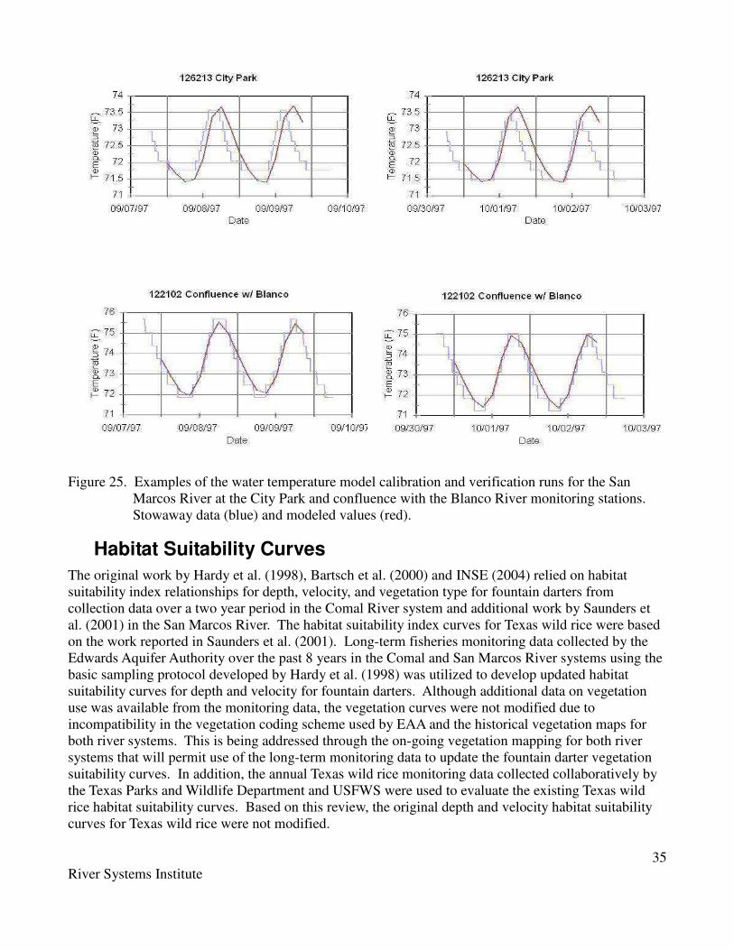
35
River Systems Institute
Figure 25. Examples of the water temperature model calibration and verification runs for the San
Marcos River at the City Park and confluence with the Blanco River monitoring stations.
Stowaway data (blue) and modeled values (red).
Habitat Suitability Curves
The original work by Hardy et al. (1998), Bartsch et al. (2000) and INSE (2004) relied on habitat
suitability index relationships for depth, velocity, and vegetation type for fountain darters from
collection data over a two year period in the Comal River system and additional work by Saunders et
al. (2001) in the San Marcos River. The habitat suitability index curves for Texas wild rice were based
on the work reported in Saunders et al. (2001). Long-term fisheries monitoring data collected by the
Edwards Aquifer Authority over the past 8 years in the Comal and San Marcos River systems using the
basic sampling protocol developed by Hardy et al. (1998) was utilized to develop updated habitat
suitability curves for depth and velocity for fountain darters. Although additional data on vegetation
use was available from the monitoring data, the vegetation curves were not modified due to
incompatibility in the vegetation coding scheme used by EAA and the historical vegetation maps for
both river systems. This is being addressed through the on-going vegetation mapping for both river
systems that will permit use of the long-term monitoring data to update the fountain darter vegetation
suitability curves. In addition, the annual Texas wild rice monitoring data collected collaboratively by
the Texas Parks and Wildlife Department and USFWS were used to evaluate the existing Texas wild
rice habitat suitability curves. Based on this review, the original depth and velocity habitat suitability
curves for Texas wild rice were not modified.

36
River Systems Institute
As highlighted above in the influence diagrams, the purpose of these effort is to establish quantitative
relationships between flow dependent attributes of depth, velocity, substrate, vegetation, temperature,
and dissolved oxygen for target species that can be used to assess available habitat within the river
systems.
The most common approach is to utilize Habitat Suitability Curves (HSC) which parametrize the
relative suitability of a factor (e.g., depth) on a scale between 0.0 and 1.0 over the range of potentially
useable values. These relationships, when combined with the hydraulic and water quality simulations
produce relationships between flow and the quantity and quality of available habitat.
Comal Springs Riffle Beetle
The Comal Springs riffle beetle (Heterelmis comalensis), is a small, aquatic beetle from the family
Elmidae known from Comal Springs and San Marcos Springs. It was first collected by Bosse in 1976
and was described in 1988 by Bosse et al. (1988). Adult Comal Springs riffle beetles are about 2 mm
(1/10 inch) long, with females slightly larger than males. The Comal Springs riffle beetle occurs in the
gravel substrate and shallow riffles in spring runs and upwelling spring orifices. Very little detailed
information is available for the Comal Springs riffle beetle. In many Elmid species, larvae undergo 6-8
instars, requiring anywhere from 6 months to 3 years to complete a life cycle from egg to adult.
Growth and development times can be temperature dependent and are faster at higher temperatures. In
other riffle beetle species, larvae crawl out of the water to construct terrestrial pupal chambers, adults
emerge and undergo a short flight period, after which they reenter the water and are incapable of
further aerial activity. However, the hind wings of Heterelmis comalensis are short and almost
certainly non-functional, making the species incapable of this mode of dispersal (Bosse et al. 1988).
Heterelmis comalensis larvae have been collected with adults in the gravel substrate of the spring
headwaters and not on submerged wood as typical of most Heterelmis species (Brown and Barr 1988).
Usual water depth in occupied habitat is 2 to 10 cm (1 to 4 inches) although the beetle may also occur
in slightly deeper areas within the spring runs. Populations are reported to reach their greatest densities
from February to April (Bosse et al. 1988). The Comal Springs riffle beetle has been collected from
spring runs 1, 2, 3, and 6 at Comal Springs in Landa Park (Bosse et al. 1988, Barr 1993) as well as the
spring orifices along the western margin of Landa Lake in the vicinity of Pecan and Spring Islands. A
single specimen was also collected from San Marcos Springs (Barr 1993). H. comalensis may have
the ability to burrow into substrate in order to avoid or tolerate environmental stress; if so, this may
explain how H. comalensis was able to survive the drought of the 1950s, when Comal Springs ceased
flowing for up to six months (Arsuffi 1993). However, genetic analysis suggests that this may have
invoked a genetic bottleneck as the genetic makeup of the recovered spring run populations differ from
populations associated with spring orifices within the bottom of Landa Lake.
The populations found in the higher elevation springs (spring runs 1, 2, and 3) of the Comal River
system contained the lowest amount of genetic variation and contained no unique haplotypes as
compared to the West Shoreline and Spring Island populations. This and the fact that the beetles are not
found in the higher elevation headwater springs (spring run 4 and 5 near Blieders Creek) could be the
result of beetle population reductions (due to bottleneck effects) in these areas due to historical
prolonged drought conditions (Gonzales 2008).

37
River Systems Institute
Stagnation of water or drying of the spring runs may be limiting conditions for the Comal Springs riffle
beetle. Flowing water is considered important to the respiration and therefore survival of these
invertebrate species. Elmid beetles have a mass of tiny, hydrophobic (unwettable) hairs on their
underside where they maintain a thin bubble of air through which gas exchange occurs. This method of
respiration loses its effectiveness as the level of dissolved oxygen in the water decreases. A number of
aquatic insects that use dissolved oxygen rely on flowing water to obtain oxygen from the water.
The technical team evaluated historical and existing distribution data for the Comal Springs riffle beetle
and believed that given the available data, the most pragmatic modeling approach was to use the total
surface area of the main spring runs (i.e., spring runs 1, 2 and 3). This was considered the most
conservative approach given the fact that they have recolonized springs that have previously gone dry.
The mechanism of recolonization (i.e., migration into the substrata or migration from other spring
sources) is not known. Modeling for the Comal Springs riffle beetle was accomplished by use of the
hydraulic model outputs within the three main spring runs of Landa Lake by summing surface areas
that were at least 0.02 feet deep. The 0.02 foot depth threshold was utilized since this is the analytical
default for the hydraulic models in the wetting and drying algorithm and therefore predicted depths
below this value are beyond the resolution of the modeling.
Texas Wild Rice
Texas wild rice habitat suitability criteria (Hardy et al. (2000) were originally generated through
examination of several papers, descriptions and existing studies. Wild rice data from TPWD
monitoring data shows wild rice to occupy moderately-coarse to coarse sandy soil sites (Poole and
Bowles 1996). This is in contrast to study results by Power and Fonteyn (1990) that found clay to be
the preferred substrate for wild rice although Power (1990) notes that in the wild: “Most Z. texana is
presently found in sandy/gravelly soil in the mid-channel of the San Marcos River.” Vaughan (1986)
found “Soil type had a minimal effect...”.
Poole and Bowles (1996) found wild rice to occur at sites with high water clarity. They also found that
salt, calcium and sulfur dioxide concentrations were higher at non-wild rice transects and hypothesized
that this was due to urban and agricultural run-off effects and the City of San Marcos Wastewater
treatment plant affect on water quality. Dissolved oxygen concentrations were found to be significantly
different between wild rice and non-wild rice areas in TPWD data (Poole and Bowles, 1996) but both
values were at oxygen saturation. Average turbidity was significantly higher for non-wild rice transects
in their study and may be a factor in downstream reaches of the San Marcos River, which can become
highly turbid from upstream recreation use on a daily basis during high use periods.
Poole and Bowles (1996) indicated that the wild rice observed depth 95% confidence intervals were
1.97 to 3.14 ft while stream locations with no wild rice had confidence intervals between 4.19 to 7.64
feet for data taken in May and August 1994 and January 1995. These averaged confidence interval
values are taken from data sets that showed significant differences in wild rice distributions. Poole and
Bowles (1996) state that, “rice transects were found to be shallower (≤ 3.2 feet) and with considerably
faster current velocities compared to non-rice transects where the water depth was greater (≥5.6 feet)
and where the current velocities were slower. Vaughan (1986) found individual wild rice stands grown
in depths greater than 0.66 feet were significantly larger (P<0.05) than those in depths less than 0.66
feet. Silveus (1933) describes wild rice as growing in water from one to seven feet deep.

38
River Systems Institute
Poole and Bowles (1996) report that average wild rice stand velocity 95% confidence intervals were
0.94 ft/s to 2.32 ft/s while non-wild rice transects had average 95% confidence intervals of 0.20 ft/s to
0.73 ft/s for data taken in May and August 1994 and January 1995. Non-wild rice areas clearly had
lower velocities than wild rice areas. Silveus (1933) describes wild rice habitat as growing “often in
swiftly running currents.”
The technical team reviewed the existing wild rice habitat suitability curves for depth and velocity used
in previous studies as well as the existing monitoring data collected over the past decade. This
included and examination of the location of persistent wild rice stands within the San Marcos system
that were overlaid on the hydraulic model solutions at different flow rates indicative of the long term
flow characteristics during the last decade. Based on this review and discussions, habitat suitability
curves were revised for use in modeling physical habitat in the San Marcos River. Figure 26 shows the
depth suitability curve, Figure 27 shows the velocity suitability curve and Table 9 provides the
corresponding HSC values used in the current analysis. Note that the curve sets labeled as ‘USFWS-
USU’ were used in the Bartsch et al. (2000) study, while the curves labeled ‘TPW’ were used in the
current report.
Depth SI Curves
0
0.2
0.4
0.6
0.8
1
0 1 2 3 4 5 6 7 8 9 10
Depth (ft)
SI
USFWS-USU
TPW
Figure 26. Texas wild rice depth habitat suitability. See text for explanation of curve legends.

39
River Systems Institute
Velocity SI Curves
0
0.2
0.4
0.6
0.8
1
0 0.5 1 1.5 2 2.5 3 3.5
Velocity (ft/s)
SI
USFWS-USU
TPW
Figure 27. Texas wild rice velocity habitat suitability. See text for explanation of curve legends.
Table 9. HSC values for depth and velocity for Texas wild rice used in the current study. These values
correspond to the TPW curves in Figures 26 and 27.
Depth
(ft) SI
Velocity
(ft/s) SI
0.00 0.00 0.00 0.13
0.10 0.00 0.10 0.13
0.15 0.26 0.15 0.27
0.75 0.26 0.20 0.27
0.80 1.00 0.25 1.00
3.00 1.00 2.00 1.00
3.05 0.48 2.05 0.30
3.75 0.48 2.50 0.30
3.80 0.36 2.55 0.12
4.50 0.36 3.00 0.12
4.55 0.24 3.05 0.00
5.25 0.24
5.30 0.04
9.00 0.04
9.05 0.00
The technical team also reviewed additional data on other factors related to the distribution and health
of Texas wild rice. In particular, it noted that Texas wild rice appears to be excluded from stream
sections with high values of canopy cover or under structures such as bridges. A relationship between
Texas wild rice suitability and the percent of canopy cover was developed but the spatial distribution of
these data is not available for the San Marcos River. Field work to obtain this data is underway as part
of on-going studies and will be incorporated into future modeling efforts supporting the development of
the HCP.

40
River Systems Institute
Fountain Darters
Previous modeling efforts for fountain darters reported in Hardy et al. (1998), Bartsch et al. (2000),
INSE (2004), and Saunders et al. (2001) relied on habitat suitability relationships for depth, velocity,
and vegetation types derived from data contained in the USFWS fountain darter biological sampling
database developed as part of those initial studies. A randomized sampling protocol was utilized using
a drop net structure based on a 3.2 foot sample grid derived from the hydrodynamic model
computational mesh (see Hardy et al. 1998). This basic approach was subsequently adopted by
monitoring activities supported by the Edward Aquifer Authority (EAA) (e.g., BioWest, 2008a).
The original studies based on drop net sampling in conjunction with scuba observations showed that
fountain dater depth use increased with increasing depth and reached a maximum at approximately 2
feet. Fountain darter use of depths less than 2 feet showed a rapid decline is numbers. Scuba
observations showed frequent use in Landa Lake at depths in excess of 10 feet. This work also showed
that fountain darters are basically associated with boundary layer hydraulic conditions (i.e., near bottom
or in velocity shelters). There is a strong negative correlation between velocity and fountain darter
habitat use. Maximum densities are most often associated with near zero velocity profiles and rapidly
decline as velocities increase. Very few observations are made at velocities in excess of 1.0 feet/second
and are basically excluded at velocities over 2.0 feet/second.
Although fountain darters can reproduce year round (Schenck, 1975), research by Brandt et al. (1993),
Bonner et al. (1998),and McDonald et al. (2007) show temperature impacts on disruption of fountain
darter life stages and underscores that temperature as a macro habitat variable is an important
component of darter habitat. These studies have shown that at temperatures between 77°F and 78.8°F,
fountain darter egg and larval survival are reduced. It is also known that egg and larval production
over 21 days are negatively impacted when daily temperatures reach these levels even if temperatures
fall within their optimum spawning range during the night. Thus, 2–3°F water temperature increase
above 75.2°F decreases fecundity and natality rates of the fountain darter.
A lower suitable temperature cutoff of 53EF is based on data from Bonner et al. (1998). Optimal
temperature ranges occur above this value and reach optimal conditions at approximately 62.6EF. This
lower temperature threshold for optimal conditions is used since 62.6EF is the lowest temperature at
which larval production was unaffected. From 62.6EF to 73.4EF, no adverse effects on darters are
known, based on the available literature. The percent hatch was lower at 77EF than at temperatures of
73.4EF (Bonner et al. 1998). The midpoint of these two temperatures, 75.2EF, was chosen as the
maximum temperature with a habitat suitability of 1.0. A reduction in temperature suitability begins
near 77EF and totally unsuitable temperatures are assumed to be reached at approximately 84.4EF. This
value was derived based on the larval LC50 of 89.6EF by invoking a conservative buffer of
approximate 4EF.
Previous modeling efforts for fountain darters reported in Hardy et al. (1998), Bartsch et al. (2000),
INSE (2004), and Saunders et al. (2001) as well as the continued critical period monitoring supported
by the EAA shows a strong correlation between fountain darter utilization of specific vegetation types.
These efforts have generally supported the original work by Schenck and Whiteside (1976) which show

41
River Systems Institute
the fountain darters prefer Rhyzoclonium sp., Hydrilla sp., and Ludwigia sp. Plant species less
preferred but still containing fountain darters are Potamogeton sp., Vallisneria sp., and Zizania sp..
Schenck and Whiteside’s (1976) sampled areas with no vegetation, and these areas were described as
not containing any fountain darters. However, diving observations in the Comal River by INSE
research staff has documented the presence of fountain darters in non-vegetated areas, albeit at lower
densities.
Given that over a decade of new sampling data was available, the technical team conducted a
multivariate analysis of the available data to provide updated habitat suitability relationships for
fountain darters. Their analysis found significant correlations between depth, velocity, height of
vegetation, and vegetation type habitat use by fountain darters, confirming the use of these variables in
the original modeling work. Although vegetation height was found to be significant, these data were
not available for all vegetation polygons within the Comal and San Marcos River systems and therefore
were excluded from the habitat modeling in the original work and the results reported here.
Based on this analysis, discussions, and temperature related research highlighted above, the habitat
suitability curves were revised for use in modeling physical habitat in the Comal and San Marcos River
systems. Figure 28 shows the depth suitability curves from the original work of Bartsch et al. (2000)
and the revised curve based on the existing analyses of available data, Figure 29 shows the velocity
suitability curve from the original work of Bartsch et al. (2000) and the revised curve based on the
existing analyses of available data, Figure 30 shows the vegetation curve, and Figure 31 shows the
temperature curve. Table 10 provides the corresponding HSC values for the revised suitability curves.
It should be noted that the vegetation suitability curve utilized in all the simulations was based on the
original curve developed by Bartsch et al. (2000) rather than the updated curve based on the analysis of
the updated data sets. This was due to incompatibility of vegetation types delineated from the original
vegetation mapping and different vegetation coding used in the EAS data sets. This will be reconciled
during the revised modeling currently underway for both the Comal and San Marcos Rivers using the
updated vegetation mapping for both systems.

42
River Systems Institute
Figure 28. Fountain darter depth habitat suitability curves (Depth_Old is Bartsch el al., (2000) and
Depth_New_Revised is derived from the analysis of the EAA monitoring data).
Figure 29. Fountain darter velocity habitat suitability (Velocity_Old is Bartsch el al., (2000)
and Velocity_New_Revised is derived from the analysis of the EAA monitoring
data).
.

43
River Systems Institute
Figure 30. Fountain darter vegetation type habitat suitability.
Figure 31. Fountain darter temperature habitat suitability.

44
River Systems Institute
Table 10. HSC values for depth, velocity, vegetation type, and temperature for Texas wild rice.
Depth
ft SI Velocity
ft/s SI Vegetation Type SI
0.00 0.00 0.00 1.00 Bare Substrate (no
vegetation) 0.05
0.03 0.00 0.03 1.00 Hydrocotyle sp. 0.20
0.66 0.02 0.23 1.00 Myriophyllum sp. 0.80
1.21 0.10 0.33 0.50 Cabomba sp. 0.40
1.48 0.20 0.39 0.20 Sagittaria sp. 0.20
1.90 0.50 0.52 0.02 Ceratophyllum sp. 0.80
2.33 1.00 0.66 0.00 Eleocharis sp. 1.00
3.51 1.00
Heteranthera sp. 0.80
3.94 0.50 Hygrophila sp. 1.00
4.36 0.20 Limnophila sp. 0.20
4.66 0.10 Ludwigia sp. 0.60
5.18 0.02 Narcissus sp. 1.00
5.81 0.00 Potamogeton sp. 1.00
Colocasia sp. 0.60
Temperature F SI Vallisneria sp. 0.80
32.00 0.00 Zizania texana 0.40
53.60 0.00 Ceratopteris sp. 0.20
62.60 1.00 Egeria (Elodea) sp. 0.20
75.20 1.00 Hydrilla sp. 0.60
80.60 0.10 Justicia sp. 0.40
84.38 0.10 Nuphar sp. 0.20
84.39 0.00 other 0.50
Physical Habitat Modeling
The Comal and San Marcos Rivers were both modeled using two-dimensional based physical habitat
modeling. This was accomplished by first assigning to each node on the computational mesh, the
associated vegetation type using GIS. For the purposes of physical habitat modeling, the nodes were
coded with the vegetation type, rather than an assigned roughness value used in the hydrodynamic
model in order to use the fountain darter vegetation type habitat suitability curve. It was assumed that
the vegetation/substrate characteristics did not change as a function of simulated flow rate. For each
modeled flow, the hydrodynamic model generates the depth and velocity at each node. As noted
previously, the hydrodynamic model utilized vegetation specific velocity equations that permitted the
adjustment of the predicted mean column velocity by vegetation type when modeling fountain darter
habitat. In the case of fountain darters, the velocity at six inches (15 cm) above the bottom was also
evaluated in the simulation of available habitat. Secondly, the water temperatures for each section of
stream derived from the QUAL2E modeling were overlain on the computational mesh and each node to
assign its respective temperature. Inclusion of temperature was specific to fountain darter assessments.

45
River Systems Institute
Comal Springs Riffle Beetle Habitat Equation
As noted previously, the technical team believes that the most conservative way to represent physical
habitat for the Comal Springs riffle beetle was total surface area within each of the main spring runs in
Landa Lake. This was accomplished by the using a binary depth suitability curve evaluated at each
node in the computational mesh within only the main spring runs of Landa Lake. This can be
represented by:
Suitability = 1.0 for Depths < 0.02 feet; otherwise Suitability = 0.0.
This binary equation was applied for all simulated flow rates within each main spring run and the total
surface area of all suitable cells were summed to derive a total habitat area as a function of flow
relationship. The results were then summed across all spring runs to derive a total habitat versus flow
relationship.
Texas Wild Rice Habitat Equation
Physical habitat for Texas wild rice was computed at each computational node using the depth and
velocity habitat criteria in a simple multiplicative manner as follows:
Suitability = DepthSI * VelocitySI
where the DepthSI and VelocitySI are computed by taking their respective values for the hydraulic
simulation results at a node and using a simple linear interpolation between the defined suitability
values from the habitat suitability index curves.
The suitability value for the computational cell was then used to multiply the cell area generating a
Weighted Usable Area (WUA) for that cell. At a given simulated discharge, all WUA values were
summed within a specific computational reach to generate a total at the reach level. Then, for each
discharge, the values were summed across all computational reaches to generate a total for the San
Marcos River at that simulated discharge.
Fountain Darter Habitat Equation
Physical habitat was computed for fountain darters using four parameters, namely depth, velocity,
vegetation type, and temperature. In the case of velocities, the mean column velocity and velocity at 6
inches (15 cm) above the bottom were used in the calculation of suitable habitat for separate analysis at
each modeled flow rate. A simple multiplicative aggregation was used as follows:
Suitability = DepthSI * VelocitySI * Vegetation_TypeSI * TemperatureSI
where the respective component suitability values are derived from a simple linear interpolation
between the the component habitat suitability relationships given these attributes at a computational
cell. The same procedures for calculation of WUA at the cell, computational reach and system wide
values were used as described for Texas wild rice above.
Modeling Results and Discussion
Physical habitat simulation results are prepared in several different formats as requested by the
technical committee. The most detail is provided by screen captures of the contoured depths and
velocities for each flow rate simulated within each of the computational segments. In addition, the

46
River Systems Institute
combined suitability for each of the target species is also provided in these formats. Summary tables
and figures are also provided for the WUA versus discharge relationships for the respective target
species. In some instances as noted below additional visualization of results are provided based on a
specific format when requested by the technical team. Given the extensive nature of the results,
summaries and illustrative examples are provided in the body of the report, while the complete results
are provided in electronic form within appendices as noted.
Comal
Temperature
Modeled temperature results for the old channel are shown in Figure 32. The old channel is a
heterogeneous stretch of stream, ranging from super critical flow in narrow sections to subcritical, slow
moving pools of water. In general, the flow behavior can be described as that of a small stream;
however at low flow rates, the surface area to volume ratio increases sharply, causing larger
temperature increases, such as those shown in Figure 32. The head of the old channel is shown on the
left, at mile 2.8. Flow goes down the old channel to mile 1.2, at which point it rejoins the new channel.
Consistent temperature increases are evident throughout the old channel at all five flow rates. At total
spring flow rates of 150 and 300 cfs (50 and 75 cfs respectively flowing down the old channel), the old
channel stream temperatures remain below 78°F. These results suggest that detrimental thermal
conditions exist in the vicinity of mile 1.95 (i.e., model segment 65), for the 60 cfs flow rate and mile
~2.25 (i.e. model segment 58) at a 30 cfs flow rate. Thus, strongly suggests that lowering the flow rate
to 60 or 30 cfs would reduce suitable darter habitat in the old channel due to temperature limitations.
Flow rates modeled within the old channel indicate that 50 cfs maintains water temperatures below
78ºF, which is close to the upper critical thermal range.
Figure 32. Simulated longitudinal temperature profile for modeled flow rate scenarios in the old
channel. Flow rates shown represent overall spring flow rates for each scenario.

47
River Systems Institute
Temperature results are shown in Figure 33 for Landa Lake, the new channel below Landa Lake, and
the Comal River proper downstream to the confluence with the Guadalupe River. Mile upstream from
the confluence with the Guadalupe River is plotted on the horizontal axis with the head of Landa Lake
being on the left side of the graph and the confluence with the Guadalupe on the right. The new
channel runs from mile 0.0 to mile 2.3, while Landa Lake runs from mile 2.3 to mile 3.4.
Figure 33. Simulated longitudinal temperature profile for Landa Lake and the new channel for
modeled flow split scenarios. Flow rates shown are total Comal River flow rates. The
letter 'A' marks significant spring locations in upper Landa Lake, the letter 'B' marks the
main spring runs, the letter 'C' marks the new channel, and the letter 'D' marks the lower
Comal River below Clemens Dam.
A general warming trend is noticeable for all flow rates, but its magnitude is minimized at larger total
flow rates of 150 to 300 cfs. Once the main spring runs and the secondary/smaller spring flows enter
the system, they cool overall river temperature. The variability in river temperature below ‘B’ in
Figure 33 is the effect of numerous medium sized spring flows entering the system immediately
upstream of the main spring runs (i.e., spring runs 1,2, and 3) within Landa Lake, which effectively
lowers the temperature.
At the upper end of Landa Lake the effect of lowering flow rates on water temperature is quite
noticeable. Increased temperatures are evident for flow rates of 30, 60 and 100 cfs. The upper
temperature threshold is reached in a progressively upstream location as flow rates drop from 150, 100,
60 and 30 cfs (i.e., at model segments 10, 7 and 1 respectively). This would potentially affect darter
reproduction from a temperature perspective in Landa Lake above the main spring runs as flows
diminish. At present, adequate information or knowledge of the effects of lower flows in conjunction
with higher summer temperatures on keystone species of the Comal River aquatic community such as
vegetation or macrocrustaceans is not available for evaluation.

48
River Systems Institute
At the higher flow rates of 150 and 300 cfs, river velocity increases, lowering retention time, and
holding down water temperatures. In reference to fountain darter reproduction, temperature is not a
limiting habitat criterion at 300 cfs. At 150 cfs, the lowest 0.7 miles of the river is estimated to exceed
78ºF, which may affect darter reproduction. The break at the end of segment ‘C’ in Figure 33 is due to
the junction of the old and new channels. Warmer water from the old channel rejoins the new channel
at this point, causing the slight jump in temperature.
The 30 cfs flow rate scenario indicates that the upper temperature threshold would occur at mile 1.42
(i.e., model segment 38), while at the 60 cfs flow rate, it would occur at river mile 0.24 or model
segment 87. The results indicated that for the 30 cfs scenario, virtually all habitat areas would exceed
this potential limiting condition, and for the 60 cfs flow scenario, potential thermally limiting
conditions to reproduction would occur by mile 2.25. These results indicate that as flows drop below
300 cfs, potential temperature limitations would begin to propagate downstream from the upper
sections in Landa Lake and in an upstream direction in the lower Comal River as a function of
decreasing flow rates.
It is evident from Figures 32 and 33 that reducing the flow rate causes temperatures in the system to
increase during late summer simulated conditions. Water temperature also increases in a downstream
direction due to decreased velocities and increased retention and travel times. Retention time is
increased further due to the large number of control structures in the system and water surface elevation
control practices.
Dissolved Oxygen
DO concentration modeling results are shown in Figures 34 and 35. DO values are generally higher
than 6 mg/L, which are attributed to reaeration within the system primarily from turbulence associated
with the hydraulic structures. It is anticipated that within Landa Lake, the upper sections of the new
channel, and the old channel downstream to the water park would likely have high DO concentrations
during the day due to the large amounts of aquatic vegetation. This may also result in depressed night
time DO concentrations under low flow conditions, especially if a large amount of the plant community
experience die offs under sustained low flow conditions.
A preliminary evaluation of the diel fluctuations at night due to the high density of aquatic vegetation
to assess DO concentrations was evaluated based on unpublished data collected by USGS in Landa
Lake in a large Vallisneria sp bed. These data showed that low DO concentrations can occur near the
stream bed in these vegetation stands even during moderate flow rates. The results suggest that at very
low flow rates and the associated higher retention times in Landa Lake with high vegetation densities
may impose DO limitations based on this preliminary data set.

49
River Systems Institute
Figure 34. Dissolved oxygen concentrations plotted against mile upstream from the end of the old
channel.
Figure 35. Dissolved oxygen concentration plotted against mile upstream from the end of the
confluence with the Guadalupe River. See text for legend explanations.
5.0
5.5
6.0
6.5
7.0
7.5
8.0
Dis
so
lve
d O
xyg
en
(m
g/L
)
1.0 1.5 2.0 2.5 3.0 Miles Upstream from Guadalupe River
Total = 300 cfs : Old channel = 75 cfsTotal=150 cfs : Old channel = 50
Total=100 cfs : Old channel = 25 cfsTotal=60 cfs : Old channel = 10 c
Total=30 cfs : Old channel = 5 cfs
Dissolved Oxygen vs. Locationin the Old Channel

50
River Systems Institute
Figure 34 reveals several patterns for DO concentrations in the old channel. At flow rates of 100, 150
and 300 cfs the DO shows a gradual upward trend with a jump in DO levels near mile 1.6. This jump
is due to channel configuration, which we call the ‘mixmaster,’ a diversion that has a significant
reaeration effect. At a total flow rate of 60 cfs (old channel flow of 10 cfs), DO concentration rises
quite rapidly due to a higher surface area/volume ratio and is near saturation concentrations and
therefore no dramatic increase is seen at the mixmaster location. At the total 30 cfs flow rate (old
channel flow of 5 cfs), DO concentrations rise rapidly at the upper end of the old channel and remain
high until higher water temperatures begin to lower the DO saturation level.
Figure 35 shows several discontinuities in DO concentrations in Landa Lake and the new channel. The
large jumps are all due to dam reaeration. Initially, DO concentrations rise over section A for flow rates
of 30, 60 and 100 cfs. This reaeration is due to the large surface area to volume ratio of upper Landa
Lake at the flow rates evaluated (i.e., 30, 60 and 100 cfs). Section B in Figure 35 shows rising DO
concentrations tempered by spring input DO levels. Comal Spring water is groundwater with low DO
concentrations typically around 4.5 mg/L. The effects of the lower DO concentrations of the spring
flows, however, is quickly attenuated within the system.
At the beginning of Section C, the main springs join Landa Lake, causing the DO concentration to drop
due to the spring water’s low groundwater DO concentrations. The jump at the end of Section C is due
to the park office weir overfall while the jump at the end of section D is due to the power plant pool
outfall. The last discontinuity in DO levels is shown at the beginning of Section F, due to the influence
of the DO concentrations from the old channel, as previously discussed
Note that the above model results were run without the effects of oxygen demanding components (e.g.,
sediment oxygen demand or plant respiration) due to lack of such calibration data. Inclusion of these
components, especially in the heavily vegetated and organic mud deposits of Landa Lake and the old
channel, would likely result in much lower daily DO concentrations due to diel DO swings. However,
the results do match calibration data at sample locations with the caveat that for the old channel only
two such sample locations existed. For each calibration time period, only one of these locations was
actively monitored. Due to the observed field values of DO, it was not felt that DO was a limiting
factor and it was not used in subsequent habitat analysis.
Comal Springs Riffle Beetle
The analysis of Comal Springs riffle beetle relied on a simple calculation of wetted surface area with
depths greater than 0.02 feet. The analysis showed no change in total surface area at total Comal River
flows between 300 and 150 cfs and then a linear reduction in available habitat below this flow
magnitude. Additional simulations were run based on criteria developed from collection data on riffle
beetles in the main spring runs as follows as an alternative to the surface area analysis.
Comal Springs riffle beetle sampling was undertaken in July and October 1993 and in January 1994
within spring runs 1, 2, and 3. The data were collected using a modified random sampling technique in
each of the four spring runs. The spring runs were split into upper, middle and lower sections. The
number of cells randomly selected within each section corresponded to a certain percentage of the area
in that section in relation to areas of other spring run sections. For example, more cells were selected
in wide runs than in narrow runs, due to differences in total surface area. Selections were aided by a
randomized listing of cells on spatially explicit maps for each spring run. During the selection process,
any selected cell sharing a side with a previously selected cell was discarded and a replacement cell
randomly selected (i.e., for a given sampling round, no sampling was done in neighboring cells). In

51
River Systems Institute
each cell, the following data were collected: spring run number, strata (section), cell number, date,
collector, start and end times, method of collection, turbidity, percentage terrestrial vegetation cover,
dominant and subdominant aquatic vegetation, organic debris type, depth and velocity, substrate codes,
and miscellaneous notes and drawings.
Sampling cells were 3.2 square feet areas. The area was sampled by placing a 3.2 foot square PVC
frame to delineate the sampling area. Sampling was by kick net method and consisted of stirring the
gravel substrate with a garden claw and capturing the debris flowing into a 12x18 inch Wildco stream
drift net with 363 micron mesh. Large rocks in the sampling area were lightly scrubbed by hand.
Samples were transferred into quart jars with 80% isopropyl alcohol for sorting in the lab. Samples
were sorted individually and numbers of adult beetles, larvae and other species were counted and
recorded.
Based on analysis of the data, the potentially suitable habitat for the riffle beetle was restricted to the
main spring runs in water depths of up to 2.0 ft and velocities of up to 2.0 ft/sec. Simulation results are
shown in Figure 36. Useable beetle habitat area varies directly with discharge as the wetted areas
containing suitable combinations of depth and velocity within the channels expand or contract. Under
low discharge conditions (< 60-100 cfs) the main spring runs 1 and 2 may cease to flow altogether
while spring run 3 decreases but flow persists, resulting in a total loss of useable beetle habitat. Spring
run 1 also loses useable area at the lowest flow rates, but remains non-zero at the lowest simulated
discharge. The combined useable areas for all spring runs show the greatest rate of decline around 100-
150 cfs.
Figure 36. Simulated Comal Springs riffle beetle habitat based on depth and velocity criteria within
spring runs 1, 2, and 3.
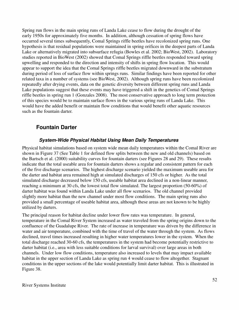
52
River Systems Institute
Spring run flows in the main spring runs of Landa Lake cease to flow during the drought of the
early 1950s for approximately five months. In addition, although cessation of spring flows have
occurred several times subsequently, Comal Springs riffle beetles have recolonized spring runs. One
hypothesis is that residual populations were maintained in spring orifices in the deepest parts of Landa
Lake or alternatively migrated into subsurface refugia (Bowles et al. 2002; BioWest, 2002). Laboratory
studies reported in BioWest (2002) showed that Comal Springs riffle beetles responded toward spring
upwelling and responded to the direction and intensity of shifts in spring flow location. This would
appear to support the idea that the Comal Springs riffle beetles migrated downward in the substratum
during period of loss of surface flow within springs runs. Similar findings have been reported for other
related taxa in a number of systems (see BioWest, 2002). Although spring runs have been recolonized
repeatedly after drying events, data on the genetic diversity between different spring runs and Landa
Lake populations suggest that these events may have triggered a shift in the genetics of Comal Springs
riffle beetles in spring run 1 (Gonzales 2008). The most conservative approach to long term protection
of this species would be to maintain surface flows in the various spring runs of Landa Lake. This
would have the added benefit or maintain flow conditions that would benefit other aquatic resources
such as the fountain darter.
Fountain Darter
System-Wide Physical Habitat Using Mean Daily Temperatures
Physical habitat simulations based on system wide mean daily temperatures within the Comal River are
shown in Figure 37 (See Table 1 for defined flow splits between the new and old channels) based on
the Bartsch et al. (2000) suitability curves for fountain darters (see Figures 28 and 29). These results
indicate that the total useable area for fountain darters shows a regular and consistent pattern for each
of the five discharge scenarios. The highest discharge scenario yielded the maximum useable area for
the darter and habitat area remained high at simulated discharges of 150 cfs or higher. As the total
simulated discharge decreased below 150 cfs, useable habitat area declined in a non-linear manner,
reaching a minimum at 30 cfs, the lowest total flow simulated. The largest proportion (50-60%) of
darter habitat was found within Landa Lake under all flow scenarios. The old channel provided
slightly more habitat than the new channel under most flow conditions. The main spring runs also
provided a small percentage of useable habitat area, although these areas are not known to be highly
utilized by darters.
The principal reason for habitat decline under lower flow rates was temperature. In general,
temperature in the Comal River System increased as water traveled from the spring origins down to the
confluence of the Guadalupe River. The rate of increase in temperature was driven by the difference in
water and air temperature, combined with the time of travel of the water through the system. As flows
declined, travel times increased resulting in higher water temperatures lower in the system. When the
total discharge reached 30-60 cfs, the temperatures in the system had become potentially restrictive to
darter habitat (i.e., area with less suitable conditions for larval survival) over large areas in both
channels. Under low flow conditions, temperature also increased to levels that may impact available
habitat in the upper section of Landa Lake as spring run 4 would cease to flow altogether. Stagnant
conditions in the upper sections of the lake would potentially limit darter habitat. This is illustrated in
Figure 38.

53
River Systems Institute
Figure 37. Total estimated fountain darter habitat in the Comal River based on physical habitat using
mean daily water temperatures. Note, suitable areas in this context reflect potential areas
below the thermal threshold at which temperatures are associated with reduced larval
survival.

54
River Systems Institute
Figure 38. Available fountain darter habitat in the Comal River at a total flow rate of 30 and 60 cfs
based on mean daily temperatures. See figure for flow rate splits in the old and new
channel. Unsuitable habitat in this context simply refers to areas at which potentially
reduced larval survival may occur.
Physical Habitat Using Maximum Daily Temperatures
Additional simulations of available fountain darter habitat in the Comal River were made based on
integration of maximum daily temperatures and hydraulic habitat (i.e., depth, velocity, and vegetation
type) based on flow splits in the old and new channel. In these simulations, only the lower part of
Landa Lake and downstream modeling sections were included since the areas upstream are not affected
by these simulations. In addition, these results include both the Bartsch et al. (2000) and revised
habitat suitability curves (see Figures 28 and 29). Table 11 shows the summary of predicted fountain
darter habitat versus discharge for various combinations of total Comal River discharges with flow
splits between the old and new channels based on both sets of suitability curves. The summary results
for the old channel are presented graphically in Figure 41 and the new channel in Figure 42 based on
the new revised suitability curves. The component results for each computational segment are
provided in tabular form in Appendix C for these simulation results.
At the request of the technical team, contour plots of the depth, velocity, and combined suitability for
fountain dater habitat were generated for each computational segment (see Figure 16). An example of
the depth and velocity contour plots (Figure 39), and the associated combined suitability for fountain
darter habitat (Figure 40) within the 'Upper Old Channel Section 2'; TopOC2 (see Figure 16) are
provided below. These figures compare the results at a flow rate of 10 and 40 cfs based on the revised
habitat suitability criteria. The results at 10 cfs show that the overall combined habitat suitability
within this section is very low (maximum of only 0.08) while at 40 cfs the maximum combined habitat
suitability increases to 0.32. The technical team examined these plots during their evaluation of flow
dependent characteristics of fountain darters throughout the system. Appendix B contains the complete
set of screen grabs for all three variables.

55
River Systems Institute
Table 11. Summary WUA relationships for fountain darters in the Comal River for simulated total
Comal River flows and corresponding flow splits between the old and new channels.
Bartsch et al. (2000) HSC Revised HSC
New
Channel
Flow (cfs)
Old
Channel
Flow (cfs)
Comal
River
Flow
(cfs)
New
Channel
WUA
(ft^2)
Old
Channel
WUA
(ft^2)
Comal
River
Total
WUA
(ft^2)
New
Channel
WUA (ft^2)
Old
Channel
WUA
(ft^2)
Comal
River
Total
WUA
(ft^2)
20 10 30 9384 4123 22361 23509 6502 44161
10 20 30 7392 3983 11376 18967 7872 25230
5 25 30 7719 3558 11277 14728 8073 21173
20 20 40 9384 2541 17547 23509 6071 39431
10 30 40 7392 3990 11383 18967 8776 26141
5 35 40 7684 3560 11244 14642 19424 32485
20 30 50 8986 3990 18599 22815 8776 39840
10 40 50 7392 3204 10596 18967 19210 36615
45 30 75 7591 3990 15945 25423 8776 41140
35 40 75 7163 3204 14729 22174 19210 48365
70 30 100 8415 3990 15232 39713 8776 54418
60 40 100 8939 3204 14422 38215 19210 61429
95 30 125 7906 3990 13776 44275 8776 56945
85 40 125 9382 3204 14407 49444 19210 72588
120 30 150 7237 3990 12518 54449 8776 65836
110 40 150 8248 3204 12576 57714 19210 80030
170 30 200 4206 3990 9121 49561 8776 60190
160 40 200 4696 3204 8598 51595 19210 72299

56
River Systems Institute
Figure 39. Depth and velocity contour plots at 10 and 40 cfs in the Upper Old Channel section of the
Comal River. Color legends are scaled between 0.0 (red) and the maximum indicated (blue)
in 10 increments of the maximum magnitude indicated.

57
River Systems Institute
Figure 40. Combined suitability for fountain darter habitat in the Upper Old Channel section of the
Comal River at 10 and 40 cfs. Legend scale is from 0.0 (red) to 1.0 (blue) in 0.1
increments.

58
River Systems Institute
Figure 41. Relationships between total Comal River discharge and simulated available habitat for
fountain darters in the old channel.

59
River Systems Institute
Figure 42. Relationships between total Comal River discharge and simulated available habitat for
fountain darters in the new channel.
These results indicate that for a given total discharge in the Comal River, increasing flow into the old
channel is somewhat insensitive to changes in available habitat, while the new channel shows a linear
response to increased habitat availability as total Comal River discharges increase. These results are
primarily attributed to the narrow range of velocity magnitudes that remain suitable for fountain darters
as illustrated in Figure 29. These results should be viewed with some caution however, given the
known channel changes within the new channel not reflected in the current analysis that includes both
topography and vegetation. These results are also cautionary in that the temperature simulations used a
spring orifice temperature as the boundary conditions for flows entering the old channel rather than the
simulated temperature at the node in Landa Lake where the culvert orifice is located. This will be
rectified in the updated modeling currently underway.
Overall, the system wide temperature simulations using both mean daily and maximum daily
temperatures strongly suggest that as total Comal River flow rates decrease, thermal affects on darter
life stages become limiting rather than the amount of physical habitat in terms of suitable depth and
velocities. The exception to this is the habitat versus flow response within the new channel which
shows somewhat rapid declines as flow rates are reduced over all ranges of simulated flows.

60
River Systems Institute
San Marcos
In this section of the report, results based on the original habitat modeling in Bartsch et al. (2000) are
provided to contrast the revised results of the current work based on updated habitat suitability curves
for fountain darters as well as changes in channel topography within the San Marcos River. These
comparisons are provided as one form of sensitivity analysis based on channel changes, differences in
habitat suitability curves, and evaluations based on both mean column velocities and velocities
estimated at 15 cm above the channel bottom. Given similarity of these two modeling approaches, only
the results for 15 cm above the bottom are presented in the report. As part of the evaluations, the
technical team was also provided with the depth and velocity contour plots at each simulated flow (see
Figure 39 above). These results are provided in Appendix D.
Temperature
Figure 43 provides a simplified overview map of the San Marcos River system utilized in the modeling
of habitat and temperature by Bartsch et al. (2000) and is used to highlight the relationship between
flow, temperature, and habitat for fountain darters within selected reaches.
Figure 44 shows the relationship between total San Marcos discharge and maximum daily temperatures
within selected reaches of the San Marcos River downstream of Spring Lake. This figure clearly
shows that as the total river discharge drops, major sections of the San Marcos have a higher potential
to cause thermal related impacts to fountain darter life stages. This is discussed in more detail in the
section on system wide fountain darter habitat below.

61
River Systems Institute
Figure 43. Major simulation reaches utilized by Bartsch et al. (2000).

62
River Systems Institute
Figure 44. Relationship between total San Marcos discharge (cfs) and reach level maximum daily
temperatures in selected reaches.
Dissolved Oxygen
Bartsch et al. (2000) did not include dissolved oxygen simulations in their modeling evaluations, nor
were they included in subsequent modeling efforts within the San Marcos River. As noted previously
for the water quality simulations for the Comal, there is concern for the potential of depressed
dissolved oxygen values during night time respiration at very low flows, especially in highly vegetated
areas such as Spring Lake and sections of the San Marcos River upstream of Cape’s Dam. If possible,
this should be addressed in the on-going modeling efforts in support of the HCP.
Texas Wild Rice
System-Wide Physical Habitat
Bartsch et al. (2000) modeled Texas wild rice throughout the Upper San Marcos River at a number of
flow rates and results are provided in Table 12. Note that these results are derived from the ‘USFWS-
USU’ habitat suitability curves shown in Figures 26 and 27. Their results are described here, while
additional modeling results specific to the Rio Vista and Cape’s Dam sections are provided below
based on the revised habitat suitability curves. The results in Table 12 indicate that Texas wild rice
habitat shows a linear increase as a function of increasing discharge for all river sections with the
exception of the Lower San Marcos A section which shows a slight decline at the highest simulated
flow rate (170 cfs). Results for specific sections are provided below.

63
River Systems Institute
Table 12. Modeled Texas wild rice habitat (WUA) by total San Marcos Spring flow rate (Bartsch et al.
2000).
Total San Marcos Springs Flow Rate
30 cfs 65 cfs 100 cfs 135 cfs 170 cfs
WUA
(ft2)
WUA
(ft2)
WUA
(ft2)
WUA
(ft2)
WUA
(ft2)
Spring Lake 0 0 0 0 55
Rio Vista 1624 3905 10524 17191 25992
Above Cape's Dam 1251 11068 25584 44043 56100
State Hatchery A 789 8341 17064 29683 32784
State Hatchery B 16 3952 14425 29714 33844
Mill Race 0 0 0 0 0
Lower San Marcos A 2206 4376 5617 7021 5748
Lower San Marcos B 0 0 0 0 2
Totals: 5885 31641 73213 127652 154525
Spring Lake
The analysis by Bartsch et al. (2000) indicated that suitable habitat in Spring Lake was negligible at all
but the highest flow rate as shown in Table 12. Their analysis of Spring Lake habitat cells’ depths and
velocities revealed that an ample amount of area existed with suitable depths for wild rice. The
velocity in each computational cell however was below the 0.87 ft/s threshold used in their wild rice
habitat suitability curve. Based in part on these results and monitoring data, Saunders et al. (2001) did
not include Spring Lake in their instream flow evaluation of the San Marcos River for Texas wild rice.
It is interesting to note that Spring Lake wild rice distribution has changed from “growth .. so luxuriant
that the irrigation company has trouble keeping the artificial lake .. clean” (Silveus 1933) to a few
scattered stands immediately below the main lake outflows where water velocities increase in this
upper section of the river system. Given these data, no further simulations of Texas wild rice were
undertaken in the present study within Spring Lake.
Rio Vista
The Rio Vista habitat section showed consistent wild rice WUA increases with increasing flow rate.
Depths decreased as flow rates dropped but never became habitat limiting within this modeled section.
This does not imply that as flow rates drop that individual Texas wild rice stands may become stranded
while suitable yet unoccupied areas are predicted to be present. Velocities were the limiting habitat
factor in the Rio Vista habitat section. Mean water velocities never reached the lower wild rice HSI
velocity threshold employed by Bartsch et al. (2000). Their analysis of modeled wild rice habitat
results showed habitat to be concentrated in the area of the University Drive Bridge at all flow rates.
Backwater effects of Rio Vista Dam tend to decrease suitable wild rice habitat due to reduced water
velocities.

64
River Systems Institute
Above Cape’s
The Above Cape’s habitat modeling section began immediately below Rio Vista Dam and continued
downstream to Cape’s Dam. This section begins as a riffle habitat type and changes to a pool/slow
moving water habitat due to Cape’s Dam backwater. Simulated water depths ranged between 3.5 feet
to 3.8 feet over the range of simulated flows within the section and were not habitat limiting with the
notable exception of several deep pools above Cape’s Dam. Simulated mean water velocities never
exceeded the minimum wild rice velocity habitat threshold values utilized by Bartsch et al. (1999) at
any of the simulated discharges.
Mill Race
Within the Mill Race habitat section, mean water depths increased from 3.5 feet to 4.9 feet as the range
of simulated discharges increased. Over the range of simulated discharges, depth was not found to a
limiting factor. Water velocities in the Mill Race were limiting to wild rice at all of the modeled flow
rates. The backwater effect of the Mill Race basically slowed water velocities to the point that no wild
rice habitat was simulated to exist in the Mill Race at any of the modeled flow rates.
State Hatchery A
Wild rice WUA consistently increased with increasing flow rates in the State Hatchery A habitat section
with increasing discharge. Mean water depths were suitable at all modeled flow rates, while water
velocities were limiting. It is interesting to note that at flow rates near the historic mean (135 cfs and
170 cfs modeled versus 148 cfs for the historic mean), mean water velocities were 0.87 and 0.95 feet
per second and at the lower range of wild rice suitability utilized by Bartsch et al. (2000). Water depths
were 3.5 feet and 3.7 feet at these modeled flow rates and at wild rice optimal depths.
State Hatchery B
The State Hatchery B section showed a consistent increase in wild rice WUA with increasing flow
rates. Water depths ranged from 1.8 feet to 2.6 feet from the lowest to highest simulated discharges.
Depths were suitable for wild rice habitat at all simulated flow rates. Suitable water velocities were
found at simulated discharges above 100 cfs, while at lower simulated discharges, low water velocity
was a limiting habitat factor in this section.
Lower San Marcos A
The Lower San Marcos A habitat segment begins at the Mill Race outfall, continues past the confluence
with the main San Marcos River channel and the City of San Marcos wastewater treatment plant input
and ends 0.8 miles downstream of the mill race/main channel confluence. This section is a transition
area from the shallower upstream reaches to the deeper Cumming’s Dam backwater found downstream.
At the lower modeled flow rates, the mean velocity in this section was below the 0.87 ft/s threshold
suitable to wild rice. Increasing the flow rate increased water velocities and consequently wild rice
WUA. As modeled flows increased from 30 to 60 cfs, the mean water depths increased to over five
feet and began to limit wild rice habitat in the simulations. This explains the decrease in wild rice
WUA at the highest flow rate of 170 cfs. The primary limiting habitat factor for the Lower San Marcos
A habitat section was water velocity.

65
River Systems Institute
Lower San Marcos B
The Lower San Marcos B habitat segment begins about 3.1 miles below Spring Lake Dam (0.8 miles
below the Mill Race/main channel confluence) and continues downstream to the confluence with the
Blanco River. This section is the deepest and slowest moving area in the San Marcos River due to
Cumming’s Dam backwater. Flow through this area is noticeably more turbid than areas further
upstream and this could be due to urban or agricultural run-off, recreation based suspension of fine
sediments, natural river processes or the combined discharges of the A.E. Woods State Hatchery and
City of San Marcos wastewater treatment plant. It is important to note that this section lies downstream
of historical wild rice distributions.
Wild rice habitat modeling shows no wild rice WUA existed at any of the modeled flow rates. The one
suitable habitat cell out of 7551 total cells at 170 cfs is considered negligible. Mean water depth in this
section ranged from 7.7 feet to 9.3 feet over the range of simulated discharges. The Lower San Marcos
B section is considered too deep and slow moving to be suitable wild rice habitat due to the backwater
effect from Cumming’s Dam.
Revised Upper San Marcos Physical Habitat Modeling
Texas wild rice monitoring data between 1998 and 2008 show only a few Texas wild rice plants below
the State Fish Hatchery (see Figure 43 for location) (unpublished TPWD/USFWS field data). Based on
this, the results presented in this section of the report focus on modeled sections upstream of that
location based on the revised habitat suitability curves (see Figures 26 and 27).
Table 13 and Figure 45 provide a comparison of estimated Texas wild rice habitat in the Rio Vista and
Above's Cape Dam sections of the San Marcos River for three different simulation results: the original
1997 geometry based simulation results, the 2001 revised geometry simulation results, and the No Dam
based geometry simulation results. The totals for these three comparisons are also provided. Figure 45
also shows the total available habitat as a percentage of maximum habitat available for illustrative
purposes.
These results suggest that Texas wild rice habitat availability is maximized in both these sections of the
San Marcos River as flow rates increase above approximately 100 cfs. They also suggest that rapid
decreases in suitable area occur below below the 65 cfs simulated flow. At 65 cfs, approximately 75
percent of maximum habitat is maintained and drops to approximately 50 percent at 30 cfs. Loss in
available habitat occurs rapidly as flows drop below 30 cfs. A comparison between the 1997 and 2001
geometry simulation results show that the implications of the measured channel changes primarily
affect the magnitude of the habitat versus flow relationships rather than a substantive change in the
underlying shape.
In contrast, the revised habitat suitability curves result in a the habitat versus flow relationships
reaching a maximum at the 135 cfs simulated discharge and then either remaining relatively constant or
show slight decreases at higher simulated flows. This is primarily attributed to the change in the depth
suitability curve (Figure 26) which shows decreased suitability between 3 and 5 feet compared to the
Bartsch el al. (2000) curves. Basically, as the flow rate increases above approximately 135 cfs, an
increasing amount of areas fall within this 3 to 5 foot range and the resulting decrease in the computed
combined suitability for Texas wild rice.

66
River Systems Institute
Table 13. Simulated Texas wild rice available habitat (Weighted Useable Area (WUA) in square feet)
in sections of the San Marcos River based on 1997 channel geometries, 2001 channel
geometries, and geometries based on assumed removal of Cape’s Dam (No Dam).
San Marcos Total
Discharge (cfs)
Rio Vista Section Above Cape’s Dam Section No Dam Total San
Marcos 1997 WUA (ft^2)
Total San
Marcos 2001 WUA (ft^2)
1997 Geometry WUA (ft^2)
2001 Geometry WUA (ft^2)
1997 Geometry WUA (ft^2)
2001 Geometry WUA (ft^2)
2001 Geometry WUA (ft^2)
15 123,570 109,550 38740 33150 55020 162,310 142,700
30 261,190 182,570 69010 46830 76110 330,200 229,400
65 351,080 307,490 110400 81720 98840 461,480 389,210
100 392,580 360,360 125480 105910 105350 518,060 466,270
135 393,250 374,390 128360 115990 105670 521,610 490,380
170 383,960 374,810 126990 118770 102050 510,950 493,580
190 350,830 118920 99980 469,750
200 339,580 115840 99090 455,420
As part of the technical team evaluations, the spatial distribution of predicted cell suitabilities were
examined on a computational cell by cell basis and compared to actual wild rice distributions based on
1989 to 2008 monitoring data at each simulated discharge. Figure 46 shows the section of the San
Marcos River in the Rio Vista to Cape’s Dam section with the simulated suitabilities for Texas wild rice
at each computational cell at a simulated discharge of 65 cfs. The known 1989 to 2008 distribution of
plant locations are overlain for comparative purposes (red dots).
The results shown in Figure 47 for the 30 cfs simulation show Texas wild rice were associated with
modeled cell suitabilities primarily below about 0.50 compared to results at 65 cfs, which show a
proportional shift with modeled cell suitabilities above 0.50. This shift in proportionally more stands
occupying modeled cells with suitabilities greater than 0.50 was observed at all higher flow rates
modeled. Observed versus use frequency distributions at flow above 65 cfs are very similar to that
reported for 65 cfs while the results for 30 cfs are indicative of the results at simulated flow lower than
30 cfs. This appears to be a systematic bias in the modeling results at lower flows that should be
examined in more detail with the revised modeling currently underway. It should also be noted that in
the simulations, the current calculations do not take into account if an existing plant species occupies
the computational element. Modeling results were also examined for locations in which the
simulations predicted suitabilities but were not occupied by Texas wild rice. Over 60 percent of these
locations were occupied by native species.
Figures 48, 49, and 50 show the contour plots of combined suitabilities for Texas wild rice in the
Above Cape’s section of the San Marcos River for flow rates of 15, 30, and 65 cfs. The plots for the
remaining simulated flows are contained in Appendix D. These results clearly illustrate the rapid loss
of suitable Texas wild rice habitat as flow decrease over these simulated flow ranges as expected from
the summary results shown in Figure 45. Future modeling efforts should increase the number of
simulated flows over these ranges to provide a better resolution of the relationship between suitable
habitat and discharge.

67
River Systems Institute
Figure 45. Simulated Texas wild rice available habitat (WUA) in sections of the San Marcos River
based on 1997 channel geometries, 2001 channel geometries, and geometries based on
assumed removal of Cape’s Dam (No Dam). The total area based on 2001 geometry is also
shown as a percent of the maximum habitat.
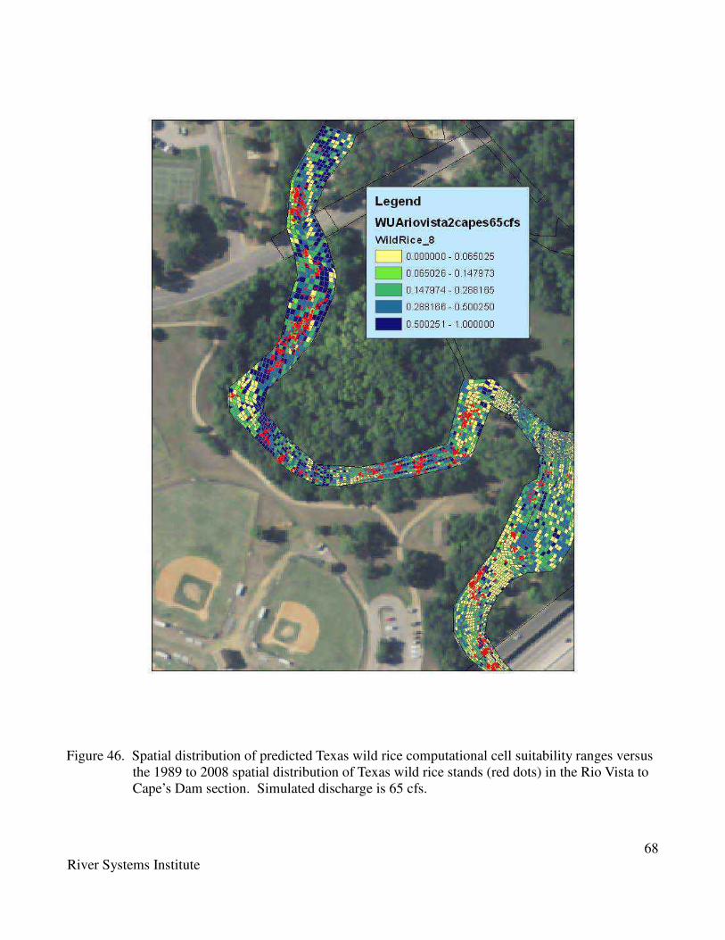
68
River Systems Institute
Figure 46. Spatial distribution of predicted Texas wild rice computational cell suitability ranges versus
the 1989 to 2008 spatial distribution of Texas wild rice stands (red dots) in the Rio Vista to
Cape’s Dam section. Simulated discharge is 65 cfs.

69
River Systems Institute
At each plant location, the computational cell estimated suitability was extracted and the frequency
distribution histogram of occupied cell suitabilities were generated. This is illustrated in Figure 47 for
a flow rate of 30 and 65 cfs.
Figure 47. Frequency histograms of simulated cell suitabilities containing Texas wild rice based at 30
and 65 cfs.

70
River Systems Institute
The technical team utilized the combined results presented above in a qualitative evaluation of
potential impacts due to recreation activities by examining the spatial locations of Texas wild rice
stands in areas with depths less than 2 - 3 feet at each simulated flow rates. It was apparent that as
flows drop below 65 cfs, proportionally greater areas in the San Marcos River were Texas wild rice
stands currently exist become more vulnerable to physical disturbance.
Texas Wild Rice Physical Habitat Summary
The simulation results indicate that over the range of simulated discharges, Texas wild rice habitat
begins to decline below approximately 100 cfs and rapidly declines below 65 cfs. Care should be taken
not to treat these specific flow rates as an 'absolute' break point given the somewhat large intervals
between simulated discharges. The results do clearly show however, that at a flow rate of 30 cfs, less
than 50 percent of maximum wild rice habitat is predicted to be available. The steepness of the habitat
versus flow relationship below the 65 cfs flow rate should however, be viewed as indicative of a rapid
decline in suitable conditions with incremental reductions in flow magnitude that 'worsens' as flow
overall flow magnitude drops . As noted in previously, revised modeling efforts should utilize a finer
scale of flow increments below the long term average to better define these habitat versus flow
responses in physical habitat.

71
River Systems Institute
Figure 48. Combined suitability for Texas wild rice habitat in the Spring Lake to Rio Vista section of
the San Marcos River at 15 cfs.

72
River Systems Institute
Figure 49. Combined suitability for Texas wild rice habitat in the Spring Lake to Rio Vista section of
the San Marcos River at 30 cfs.

73
River Systems Institute
Figure 50. Combined suitability for Texas wild rice habitat in the Spring Lake to Rio Vista section of
the San Marcos River at 65 cfs.

74
River Systems Institute
Fountain Darter
System-Wide Physical Habitat
Summary results for fountain darter physical habitat simulations based on Bartsch et al. (2000) are
provided in Table 14 (see Figure 43 for locations). Updated simulation results are presented below
based on both changes in the channel topography and updated habitat suitability curves. These later
simulations however, rely on the original temperature simulations results shown above.
Table 14. Simulated fountain darter habitat within sections of the San Marcos River for selected flow
rates after Bartsch et al. (2000).
Total San Marcos Springs Flow Rate
30 cfs 65 cfs 100 cfs 135 cfs 170 cfs
WUA
(ft2)
WUA
(ft2)
WUA
(ft2)
WUA
(ft2)
WUA
(ft2)
Spring Lake 218760 239751 255885 258495 263163
Rio Vista 77633 151422 185614 220996 229134
Above Cape's Dam 46335 54197 60143 56240 51181
State Hatchery A 4524 13934 15442 16136 11782
State Hatchery B 1483 3702 3107 3052 1707
Mill Race 26572 37368 44886 47040 45698
Lower San Marcos A 19159 22343 25970 24025 21844
Lower San Marcos B 69780 78308 76482 72867 69056
Totals: 464245 601026 667530 698851 693565
Spring Lake
An analysis of the fountain darter WUA results revealed that the Spring Lake slough area had poor
fountain darter WUA values at all modeled flow rates. Depths and velocities were in suitable ranges
but mean water temperatures were above the 75.2 F upper threshold for suitable thermal conditions.
This was attributed to lack of flow coming down the Sink Creek channel through the slough. The
average water temperature was always at the upper limit of useable temperatures for the fountain
darter, and at a temperature which may impact fountain darter breeding. Field observations have
shown the slough to become a vegetation-choked backwater area with extremely low flow and elevated
temperatures, confirming the modeling result. Note that the slough area is only wetted due to the Spring
Lake Dam backwater and does not contain any major springs.
The non-slough area of Spring Lake showed slightly decreasing fountain darter WUA as flow rates
decreased. Water depths remained fairly constant due to the Spring Lake Dam backwater and had little
effect on fountain darter WUA. Water velocities were extremely slow at all modeled flow rates due to
the backwater effect and were not a limiting factor. Water temperatures increased as flow rates
decreased and became the limiting habitat factor below 65 cfs. The lowest part of Spring Lake receives
the combined flows of the springs area and the slough and was more prone to high temperatures as flow
rates were lowered. Overall Spring Lake fountain darter WUA showed a consistent decrease as flow
rates decreased.

75
River Systems Institute
Rio Vista
Habitat modeling results showed consistently increasing fountain darter WUA with increasing flow
rates. The WUA for 135 cfs and 170 cfs modeled total San Marcos Springs flow rates were about the
same. It should be noted that the Rio Vista and Mill Race sections contained the highest aquatic
vegetation aerial coverage, although Rio Vista section had much more vegetative diversity than the Mill
Race section. This was of overall benefit to the fountain darter as areas with little vegetation had low
HSI values for fountain darters as noted previously.
Water temperatures increased as modeled flow rates decreased and were of moderate importance as a
habitat-limiting factor. Mean water depths in the Rio Vista habitat section fell below the two foot
threshold between 30 cfs and 65 cfs and began to limit fountain darter WUA. Mean water velocities in
this section never rose above the 0.5 ft/s threshold at which they would have become habitat-limiting.
Overall fountain darter WUA was limited by depths and temperatures at low flowrates for the Rio Vista
Dam habitat section.
Above Cape’s
The Above Cape’s habitat modeling section starts immediately below Rio Vista Dam and
stretches downstream to Cape’s Dam. Habitat at the upper boundary is characterized by fast, shallow
water while habitat further downstream is dominated by Cape’s Dam backwater and has low velocity
and increased depths (up to 17 feet just above Cape’s Dam). This lower section exhibited a diverse
range of vegetation species beneficial to fountain darter use. Mean water depths in this section were
3.46 feet at the lowest flow rate modeled and increased as flow rates increased, never becoming habitat
limiting for fountain darters. Water temperatures increased at lower flow rates and became habitat
limiting at modeled flow rates of 65 cfs and below.
Mill Race
The Mill Race section had high vegetation aerial coverage and in particular was dominated by hydrilla,
a non-native plant that is favorable to fountain darter utilization. The dominance of hydrilla in the Mill
Race area led to high fountain darter WUA estimates when temperatures and velocities were not
limiting. As flow rates decreased, fountain darter WUA decreased in the Mill Race section. Mean
water velocity in this section never exceeded the 0.5 ft/s threshold at which it would have become
limiting. Depths throughout this section did not vary much with discharge due to the Mill Race outfall
backwater and were never limiting over the range of simulated discharges. Water temperatures
increased in the Mill Race habitat section and became the limiting factor for fountain darter habitat
below 65 cfs.
State Hatchery A
The State Hatchery A habitat segment starts in the main channel of the San Marcos River just below
Cape’s Dam and runs 0.45 miles downstream to the County Road Bridge, with the last 0.1 miles of the
section characterized by fast, shallow water rapids by Bartsch et al. (2000). The section was sparsely
vegetated and this lack of vegetation limited predictions of available fountain darter habitat. As with
other sections, water temperatures rose as flow rates decreased, reducing the overall suitability of
fountain darter habitat. Depths were not a limiting factor at any of the simulated discharges. However,
in sections with higher gradients, increasing areas with simulated velocities were above the 0.5
feet/second threshold set for suitable fountain darter habitat as simulated discharges increased.

76
River Systems Institute
State Hatchery B
The State Hatchery B habitat section was composed of the main channel of the river from County Road
Bridge downstream to the confluence of the Mill Race outfall. This section receives the A.E. Woods
State Fish Hatchery discharge about 300 feet upstream from its lower boundary. This section is of
moderately high gradient and characterized by shallow, fast flowing water. Vegetation coverage
throughout was sparse and comprised mainly of elephant ear and hydrilla. Fountain darter WUA in
this section was limited by this lack of aquatic vegetation (only 457 habitat cells of 4995 total habitat
cells, or 9%, had vegetation of any sort according based on the vegetation mapping data) and the
resulting WUA value magnitudes were low. Mean water depths at simulated discharges below 65 cfs
were below the 2.0 foot lower threshold of suitable fountain darter habitat. As in other sections, water
temperatures became limiting below 65 cfs. In summary, the State Hatchery B habitat section was
limited by depth, velocity, vegetation, and temperatures. Increased water temperatures and decreased
depths limited fountain darter WUA at lower modeled flow rates, while increased water velocities
limited fountain darter WUA at higher modeled flow rates, and lack of vegetation limited fountain
darter WUA at all flow rates.
Lower San Marcos A
The Lower San Marcos A segment showed no clear pattern in fountain darter WUA. The adverse
effects of elevated water temperatures at lower flow rates were balanced by the adverse effects of
increased velocities at higher flow rates with the 100 cfs modeled discharge being the break point
between these competing effects. Mean water depths in this section were sufficiently deep (4.3 feet at
the lowest modeled flow rate) and were not habitat limiting over any range of simulated flows. This
river section had very sparse vegetation coverage based on the vegetation maps utilized, limiting
fountain darter WUA. Areas with no vegetation have minimal fountain darter habitat value.
Lower San Marcos B
The Lower San Marcos B habitat section had the lowest vegetation density of any San Marcos habitat
modeling section. Only 0.8% of habitat cells (51 of 7551 total) had vegetation according to the
vegetation mapping. Mean water depths through this area were the deepest in the San Marcos River
due to the backwater from Cumming’s Dam and were not limiting any simulated discharge. This
section of the San Marcos River had lower diel temperature fluctuation amplitudes than any of the
upper San Marcos River reaches. Bartsch et al. (2000) attributed this result to greater thermal mass
which acts as a buffer against day-and-night temperature variations. Temperatures fluctuated around
3°F at all flow rates in this section as opposed to up to 8°F in the Rio Vista habitat section at flow rates
below 65 cfs. The limiting habitat factor for fountain darters in the Lower San Marcos A section was
lack of vegetation. Fountain darter WUA increased slightly at higher flow rates due mainly to lowered
temperature effects.
Upper San Marcos Physical Habitat
This section of the report highlights fountain darter habitat simulations in the reaches of river upstream
of Cape’s Dam. These results are used to explore sensitivity of simulation results to such factors as
channel changes and suitability curves.

77
River Systems Institute
The relationship between available simulated habitat for fountain darters versus discharge for the
simulated scenarios in the upper section of the San Marcos River are provided in Table 15 and Figure
51. Figures 52, 53, and 54 illustrate examples of the contour plots of combined suitabilities for
fountain darters in the Spring Lake to Rio Vista section of the San Marcos River for flow rates of 15,
30, and 65 cfs. These plots for the remaining simulated flows and other key river sections are
contained in Appendix D and are based on the updated habitat suitability curves for fountain darters.
Table 15. Simulated fountain darter available habitat in selected sections of the San Marcos River
based on 1997 channel geometries, 2001 channel geometries, and geometries based on
assumed removal of Cape’s Dam (No Dam). The 2009 results are based on revised habitat
suitability curves.
San Marcos Total Discharge
(cfs)
Rio Vista Section Above Cape’s Dam
Section No Dam
Total San
Marcos 1997
Total San
Marcos 2001
Rio Vista 2009 WUA
Above Cape's Dam 2009 WUA
Total San
Marcos 2009
1997 Geometry
WUA
2001 Geometry
WUA
1997 Geometry
WUA
2001 Geometry
WUA
2001 Geometry
WUA
15 48420 50700 38720 38480 13250
87140 89180 42620 36870 79490
30 89830 89170 47640 49870 17460
137470 139040 70210 47250 117460
65 174210 156020 64930 68520 22750
239140 224540 109210 55050 164260
100 188410 179710 65870 68620 22610
254280 248330 97790 40760 138550
135 197270 183320 64280 64910 22480
261550 248230 75660 22880 98540
170 188300 174840 63220 62350 22940
251520 237190 56800 15880 72680
190 179060 52800 22180
231860 54460 11440 65900
200 179060 58760 21760
237820 51640 11950 63590
These results show that habitat availability decreases most rapidly at flow rates below 65 cfs regardless
of the channel geometry utilized or the habitat suitability curves used in the modeling. The revised
suitability curves used for the ‘2009’ simulations (see Figures 28 and 29), which show a very narrow
range of velocity magnitudes that are suitable as well as requiring somewhat deeper water for suitable
conditions results in a habitat versus flow relationship that is more ‘peaked’ around the maximum
values at 65 cfs. The is primarily attributed to higher velocities limiting apparent fountain darter
habitat as flow rates increase above the 65 cfs simulated flow. It should be noted however, that
maximum habitat may in fact occur at flow rates between 65 and 100 cfs and a more refined increment
of flow simulations will be utilized in the updated modeling.

78
River Systems Institute
Figure 51. Simulated fountain darter available habitat (WUA) in sections of the San Marcos River
based on 1997 channel geometries, 2001 channel geometries, and geometries based on
assumed removal of Cape’s Dam (No Dam).
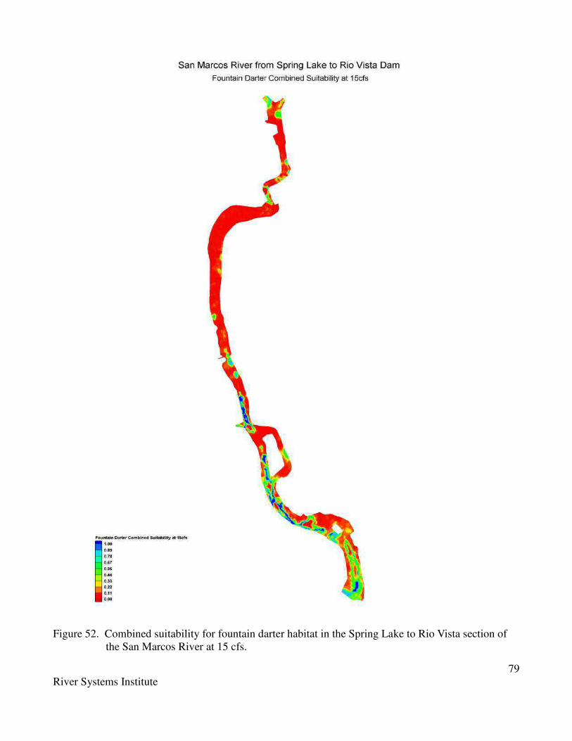
79
River Systems Institute
Figure 52. Combined suitability for fountain darter habitat in the Spring Lake to Rio Vista section of
the San Marcos River at 15 cfs.

80
River Systems Institute
Figure 53. Combined suitability for fountain darter habitat in the Spring Lake to Rio Vista section of
the San Marcos River at 30 cfs.
81
River Systems Institute
Figure 54. Combined suitability for fountain darter habitat in the Spring Lake to Rio Vista section of
the San Marcos River at 65 cfs.

82
River Systems Institute
Sensitivity to Channel Change and Habitat Suitability Criteria
These results are used to illustrate modeling sensitivity to channel changes versus habitat suitability
curves as illustrated in Figure 55 which plots data from Figure 51 as the percent of maximum habitat
values. These results show that the measured channel changes between 1997 and 2001 do not alter the
underlying habitat versus flow relationship. It should be noted that these two comparisons only reflect
changes in the topography of the computational mesh and the not revisions in the fountain darter
habitat suitability functions. The results from the 2009 simulations based on the 2001 channel
topographies (2001 Geometry with New HSC) reflect the updated fountain darter habitat suitability
relationships. As can be seen, the changes in habitat suitability curves for fountain darter not only
changed the magnitude of simulated habitat versus discharge relationship (Figure 51) but also changed
the underlying habitat versus flow relationship. As noted previously, this is primarily attributed to the
differences in the velocity suitability curve (see Figure 29).
Figure 55. Relationship between total San Marcos river discharge and simulated available fountain
darter habitat as a percent of maximum habitat.
83
River Systems Institute
Fountain Darter Physical Habitat Summary
It is apparent from a comparison of these simulation results that the combined effect of channel change
and differences in habitat suitability curves for fountain darters can shift the flow rate at which habitat
is maximized. The results (see Table 15) also illustrate that these factors show a differential response by
specific river reach. However, it is clear that regardless of these simulation differences, fountain darter
habitat quantities show declines within the San Marcos River as flow rates drop below about 65 cfs. It
is cautioned however, that more simulated flows between the 65 and 30 cfs flow range are needed in
the revised modeling currently underway to better define where this rapid decline in available habitat
begins.
Other Native Aquatic Species
In addition to the three target species that are the focus of the quantitative assessments presented above,
a number of other native species inhabit the Comal and San Marcos Rivers. In this section of the report
several key species are highlighted and discussed in light of the results from the existing modeling.
Comal Springs dryopid beetle (Stygoparnus comalensis)
The Comal Springs dryopid beetle is considered to be primarily a subterranean species, although it has
been collected from all six spring runs and springs located along the western margin of Landa Lake
(Barr and Spangler 1992, Randy Gibson personal communication). Given its subterranean distribution
and use of spring runs, it is likely not significantly impacted by changes in spring flow discharge.
Assuming that flow regimes are maintained in the Comal River such that spring discharges are
maintained to protect the Comal Springs riffle beetle and fountain darters, adequate protection would
be maintained.
Peck’s cave amphipod (Stygobromus pecki)
Peck's cave amphipods have been collected from all six spring runs and springs located along the
western margin of Landa Lake (Arsuffi 1993, Barr 1993, Randy Gibson personal communication).
This species appears to be primarily a subterranean species with limited distribution within spring runs.
No quantitative data is available on its life history requirements. As noted for the Comal Springs
dryopid beetle, maintenance of spring flow in the Comal River system would likely provide adequate
protection for this species. However, it is noted that periodic drying may not result in large impacts due
to its subterranean distribution.
San Marcos Gambusia (Gambusia georgei)
The San Marcos gambusia has not been collected since 1982 and is most likely extinct (USFWS 1996).
The mechanisms responsible for the decline and apparent extirpation are not known but hybridization
with the western mosquitofish (G. affinis) and loss of suitable habitat along the stream margins due to
invasion of the exotic macrophyte elephant ears (Colocasia esculenta). It is assumed that if adequate
flow regimes exist for the protection of fountain darters, suitable hydrologic and water quality
conditions would be maintained for this species.

84
River Systems Institute
Texas blind salamanders (Eurycea rathbuni)
Texas blind salamanders are distributed throughout the aquifer in the San Marcos region of the
Edwards Aquifer. Given their subterranean distribution with the aquifer, maintaining spring flows
within the San Marcos River would likely ensure flow related protection for this species. However,
continued protection of groundwater water quality remains a concern given the projected increases in
population density within this region.
San Marcos salamanders (Eurycea nana)
San Marcos salamanders (Eurycea nana) have been reported throughout Spring Lake and up to ~ 500
feet below Spring Lake Dam (Nelson 1993). They appear to prefer areas with silt free rocks associated
with spring openings, silt free rocky substrates within the main channel of the San Marcos River, and
are associated with filamentous algae within Spring Lake. Although it appears that populations within
Spring Lake would be protected as long as adequate spring flows are maintained, populations within
the downstream channel of the San Marcos River are at risk from both reduced flow rates and
recreation activities.
Cagle’s map turtle (Graptemys caglei)
The Cagle's map turtle is distributed within areas of the Guadalupe and lower San Marcos Rivers in
Kerr, Kendall, Comal, Guadalupe, Gonzales, DeWitt, Hays, and Victoria Counties (Killebrew et al.
2002) and is a candidate for listing by the USFWS. Maintaining adequate spring flow regimes for
protection of Texas wild rice and fountain darters will likely contribute to suitable flow and water
quality conditions in these downstream reaches.
Non-native Species
Non-native species are a concern in both the Comal and San Marcos River systems. These include
mammals, aquatic plants, snails, parasites, and fish species. In most cases, the direct or indirect
impacts to native flora and fauna are not known. This section of the report highlights several non-
native species that are known or suspected of having potential impacts to the key target species. Tables
16 and 17 provide a list of the fish collected from the Comal and San Marcos River systems as part of
on-going critical flow monitoring supported by the Edwards Aquifer Authority.
The list of species within the Comal and San Marcos Rivers include several potential native and non-
native predators. However, the extent to which predation may be limiting fountain darters is unknown.
Long-term monitoring of fountain darter populations over moderate to high flow rates do not indicate
predation as a major factor, but may be more problematic at low discharges when spatial segregation
becomes more difficult. This could be exacerbated with low flows and loss of aquatic vegetation
density (and diversity) that fountain darters rely on for habitat selection. The broader impacts of
introduced species in terms of alteration of trophic pathways, competition of food resources, etc. is
basically unknown at this time.

85
River Systems Institute
Suckermouth Catfish (Hypostomus sp.)
A concern has arisen given the apparent high density of suckermouth catfish which are herbivorous. At
high densities, indirect impacts to fountain darters may occur due to large scale alterations in the
aquatic vegetation density and composition upon which fountain darters are dependent. Physical
alteration of the stream banks due to burrowing is also a concern with large trees being felled due to
bank instability. This can indirectly affect water quality by increased sediment inputs. This would also
affect Texas Wild rice directly through herbivory and indirectly when downed trees scrape the river
bottom during flood events.
Table 16. List of fish taxa and number collected from the Comal River between 2001 and 2007.
Adapted from Bio-West (2008a).

86
River Systems Institute
Table 17. List of fish taxa and number collected from the San Marcos River between 2001 and 2007.
Adapted from BioWest (2008b).
Tilapia (Tilapia sp.)
Landa Lake is known to support an increasing population of tilapia. This species is omnivorous with a
preference for aquatic vegetation and detritus. As noted for the suckermouth catfish, indirect affects
from alteration of the aquatic vegetation community are of concern.
Nutria (Myocastor coypus)
Nutria are found both in the Comal and San Marcos River systems. However, very little work has been
undertaken to examine their potential impacts on native species within these river. Nutria may cause
direct and indirect impacts through destruction of aquatic vegetation and eroding river banks. It is
speculated that if river flows in these systems are severely reduced, potentially significant impacts may
occur due to alteration of vegetation preferred by fountain darters thereby reducing overall habitat
availability and quality. Nutria have been observed eating Texas Wild rice.

87
River Systems Institute
Elephant Ears (Colocasia esculenta)
Vegetation monitoring has shown the distribution and density of Elephant Ears is increasing in some
sections of both river systems. This invasive species does not provide high quality habitat for fountain
darters and can completely exclude wild rice stands. In addition, its broad aerial leaf morphology
results in very high transpiration rates, which at lower discharges has the potential to impact low flow
regimes.
Giant Ramshorn Snails (Marisa cornuarietis)
Giant Ramshorn snails have periodically been a concern due to their ability to significantly alter the
density and composition of the aquatic vegetation community. Although the Giant Ramshorn snail has
been known from the Comal Springs system since about 1983, they reached very high density in the
later 1980s and significantly reduced vegetation stands in Landa Lake (Horne et al. 1992, Linam et al.
1993). However, by the early 1990s, populations underwent a significant decline. The mechanisms for
their increased density may have been associated with sustained lower than normal flows, while their
decline may have been related to over crowding in conjunction with higher sustained spring discharges
(Horne et al. 1992). Population densities at present are low, but appear to be increasing with the
sustained low flows within the Comal River (Tom Brandt, personal communication). At present,
populations in the San Marcos River are at very low numbers.
Asian snail (Melanoides tuberculata)
The primary concerns with the Asian snail are its impact on native vegetation and as an intermediate
host for the gill parasite (Centrocestus formosanus) on fountain darters. Population increases appear to
be related to sustained low flows which in turn can lead to increases in the abundance of gill parasites
(Tom Brandt, personal communication).
Gill Parasite (Centrocestus formosanus)
Increasing concern has arisen over the impact of the gill parasite on fountain darters. Infection of
fountain darters has been traced to cercariae emerging from the exotic red-rimmed melania snail,
Melanoides tuberculata. Impacts include direct mortality from heavy infestation and sub-lethal effects
due to stress. Bolick (2007) reported that neither total stream discharge (USGS gauge) nor wading
discharge (measured at each transect when collections were taken) were found to be a useful predictor
of cercarial abundance. However, historical field observations in the Comal River indicate that
abundance is related to sustained low flows in combination with above average water temperatures
(Tom Brandt, USFWS, personal communication). Recently, increased infection rates within the San
Marcos River have been reported and may be related to the lower sustained discharges during the 2008-
2009 drought (Tom Brandt, personal communication and unpublished field data).

88
River Systems Institute
Recreation
As noted in the results section for Texas wild rice, the primary factors considered from the results of the
existing modeling was a qualitative evaluation of Texas wild rice locations that would 'be at risk' from
shallow depths (< ~ 3 feet) as flow rates drop in the San Marcos River. These risks primarily focus on
physical disturbance. However, observations during the original studies cited in this report as well as
on going monitoring activities for Texas wild rice clearly show that as recreation intensity increases on
a given day, the downstream turbidity dramatically increases in both the Comal and San Marcos River
systems. Anthropogenic suspension of fine sediments can be severe enough to preclude visual
delineation of wild rice stands in the lower San Marcos River in the afternoon during high recreation
use periods (Jackie Poole, personal communication). Field observations by the author while diving in
both the Comal and San Marcos River systems showed that in the lower extents of both rivers, fine
particulate matter completely covered the submerged aquatic vegetation. The extent to which the
suspended sediment and physical sedimentation may be inhibiting Texas wild rice (or other native
aquatic species) is unknown. Recreational activities also have the potential to affect fountain darter
through direct and indirect impacts. Direct effects include tramping and continual displacement of
individuals in high use areas. Indirect impacts include reduction of suitable habitat areas due to
disturbance or complete loss of specific vegetation types preferred by fountain darters. It is anticipated
that these effects are likely to be exacerbated during low flow conditions but could be mitigated
through aggressive recreation control measures.
Summary
Historical and updated modeling of water quality (temperature and dissolved oxygen) and physical
habitat for Texas wild rice, Comal Springs riffle beetle, and fountain darters have been summarized for
use by the Expert Science Committee of the Edwards Aquifer Recovery and Implementation Program.
Updated habitat suitability curves for fountain daters were developed based on a analysis of available
monitoring data. Data visualization and summary results were prepared based on input from members
of the Expert Science Committee as well as other knowledgeable scientists familiar with these target
species and the Comal and San Marcos River systems.
Physical habitat modeling involved the application of two-dimensional hydrodynamic models to
estimate the distribution of available depths and velocities as a function of simulated flow rate for
specific sections of both the Comal and San Marcos Rivers. Temperatures were derived from the
QUAL2E model reported in Bartsch et al. (1999) and Hardy et al. (1998) for the San Marcos River and
Comal Rivers. These data were used in combination with habitat suitability curves for depth and
velocity to estimate available habitat for Texas wild rice and the Comal Springs riffle beetle over a
variety of flow rates. Fountain darter habitat was modeled using depth, velocity, vegetation type, and
temperature. Vegetation distribution for each river was taken from historical vegetation mapping
results. Fountain darter habitat suitability curves were derived from a multivariate analysis of long
term monitoring data from the Comal and San Marcos Rivers.
Detailed contour plots of the combined suitability derived from the component suitabilities of depth,
velocity, vegetation type and temperature (as appropriate) for Texas wild rice and fountain darters were
developed for each modeled river section for the the Comal and San Marcos Rivers at each simulated
discharge. In addition, summary relationships between predicted available habitat discharge were
developed. Finally, modeling sensitivity to changes in channel topography and habitat suitability
curves are provided.

89
River Systems Institute
Future Study Recommendations
• The current efforts to remodel by the Comal and San Marcos River systems should be
undertaken with a single hydrodynamic model. This will allow for easier technology transfer
and allow a consistent analysis framework.
• It is also recommended that a single water quality model be applied in both river systems for
these same reasons. The model should simulate maximum daily temperatures and be applied
system-wide for both rivers.
• Water quality modeling should consider non-point and point source pollutants to the extent
these inputs can be approximated from available data.
• Analysis of alternative species beyond the three target species focused on in this report should
also be undertaken. The specific species to be included should be determined after an analysis
of the existing long-term monitoring data available for both river systems.
• Consideration should be given the potential vegetation changes if possible since vegetation
responses to flow regime changes are critical to evaluation of available fountain dater habitat.
• A quantitative assessment of potential impacts associated with recreation should be considered
that includes not only Texas wild rice but other aquatic vegetation.
• Analysis of channel topography changes due to fine sediment input should also be considered if
possible.
• A finer resolution on the number of simulated flows is also important, especially for flow ranges
below the average annual flow to better inform decisions on critical flow management.
• Refinement in the total Comal River discharge versus specific spring flow rates and flow rates
at which specific springs cease to flow should be undertaken.
• Texas wild rice habitat simulations should be modified to account for computational cells
occupied by other species.
• If feasible, system wide substrate mapping in the San Marcos “under” existing vegetation stands
should be considered to allow evaluation of non-native plan removal on providing suitable
Texas wild rice habitat beyond a depth and velocity evaluation.
• Evaluate the potential of including anthropogenic induced turbidity on light attenuation as a
function of the longitudinal profile of the river systems and its implication on vegetation.

90
River Systems Institute
References Cited
Armour, C.A. 1991. Guidance for Evaluating and Recommending Temperature Regimes to Protect
Fish. Instream Flow Information Paper 28. U.S. Department of the Interior, Fish and Wildlife
Service, Washington, D.C. 20240.
Arsuffi, T.L. 1993. Status of the Comal Spings riffle beetle (Heterelmis comalensis), Pick’s cave
amphipod (Stygobromus pecki), and the Comal Springs dryopid beetle (Stygoparnus
comalensis): Prepared for the U.S. Fish and Wildlife Service, 25 p.
Barr, C. B. 1993. Survey for two Edwards Aquifer invertebrates: Comal Springs dryopid beetle
Stygoparnus comalensis Barr and Spangler (Coleoptera: Dryopidae) and Peck’s Cave amphipod
Stygobromus pecki Holsinger (Amphipoda: Crangonyctidae). Prepared for U.S. Fish and
Wildlife Service, Austin, TX.
Barr, C.B. and P.J. Spangler. 1992. A new genus and species of stygobiontic dryopid beetle,
Stygoparnus comalensis (Coleoptera, Dryopidae), from Comal Springs, Texas. Proceedings of
the Biological Society of Washington 105(1):40-54.
Bartsch, N.R., T.B. Hardy, J.A. Shoemaker, and P.J. Connor. 2000. Development and Application of an
Instream Flow Assessment Framework for the Fountain Darter (Etheostoma fonticola) and
Texas Wild rice (Zizania texana) in Spring Lake and the San Marcos River System.
Bartsch, N. R. 1996. Development and utilization of a physical habitat model for Etheostoma fonticola
in the Land Lake and Comal River systems. M.S. Thesis. Utah State University, Logan, Utah.
Beaty, H.E. 1975. Texas Wildrice. Texas Horticulturist 2(1):9-11.
BioWest. 2002. Comal Springs riffle beetle laboratory study: evaluation under variable flow conditions.
Final Report. Edwards Aquifer Authority, San Antonio, Texas. 22p.
BioWest. 2008a. Comprehensive and critical period monitoring program to evaluate the effects of
variable flow on biological resources in the Comal Springs/River aquatic ecosystem. Final
2007 annual report. Edward Aquifer Authority. 48pp. + appendices.
BioWest. 2008b. Comprehensive and Critical Period Monitoring Program to Evaluate the Effects of
Variable Flow on Biological Resources in the San Marcos/River Aquatic Ecosystem. Final 2007
Annual Report. March 2008. 3pp + appendices.
Bolick, A.E. 2007. The effects of spring flow on the abundance of the Heterophyid cercariae in the
Comal River, New Braunfels, Texas. M.S. Thesis, Texas State University. 48 pp.
Bonner, T.M., T.M. Brandt, J.N. Fries, and B.G. Whiteside. 1998. Effects of temperature on egg
production and early life stages of the fountain darter. Transactions of the American Fisheries
Society 127: 971 – 978.
Bosse, L.S., D.W. Tuff and H.P. Brown. 1988. A new species of Heterelmis from Texas-(Coleoptera,
Elmidae): Southwestern Naturalist, v. 33, no. 2, p. 199-204.
Bovee, K.D. 1978. The incremental method of assessing habitat potential for coolwater species with
management implications. American Fisheries Society Special Publication 11:340-346.
Bowles, D.E., R. Stanford and C.B. Barr. 2002. Habitat and phenology of the endangered riffle beetle
Heterelmis comalensis and a coexisting species, Microcylloepus pusillus, (Coleoptera: Elmidae)
at Comal Springs, Texas, USA: Archiv fur Hydrobiologie, 156(3): 361-383.
Brandt, T.M., K.G. Graves, and C.S. Berkhouse. 1993. Laboratory spawning and rearing of the
endangered fountain darter. Progressive Fish-Culturist 55:149-156.
Brown, L.C., and T.O. Barnwell. 1987. The enhanced stream water quality models QUAL2E and

91
River Systems Institute
QUAL2E-UNCAS: Documentation and users manual. Medford: Tufts University, Department
of Civil Engineering (EPA/600/3-87/007).
Brown, H.P., and C.B. Barr. 1988. First report of stygobiontic (subterranean) riffle beetles in North
America: Program abstract for April 22, 1988, meeting of Southwestern Association of
Naturalists, 5 p.
Brune, G. B.1981. Springs of Texas, Volume I. Branch-Smith, Inc. Fort Worth, Texas. 566 pp.
Buckner, H.D. and W.J. Shelby. 1990. Water resources data for Texas, Water Year 1990, Volume 3;
Colorado River Basin, Lavaca River Basin, Guadalupe River Basin, Nueces River Basin, Rio
Grande River Basin, and Intervening Basins. Austin, TX: U.S. Geological Survey (Water Data
Report TX-90-3).
Conservation Breeding Specialist Group. 1997. San Marcos and Comal Springs Ecosystems Viability
Assessment and Management Planning: Texas Wild rice Working Group Discussion Notes
(Revised).
Emery, W.H.P. and M.N. Guy. 1979. Reproduction and embryo development in Texas wild rice
(Zizania texana Hitch.) Bull. Torrey Botanical Club 106:29-31.
Emery, W.H.P. 1981. Status of Texas wild rice. Notes from USFWS files.
Gandara, S.C., W.J. Gibbons, D.L. Barbie, and R.E. Jones. 2000. Water Resources Data Texas Water
Year 1999. Vol. 5 Guadalupe River Basin, Nueces River Basin, Rio Grande Basin, and
Intervening Coastal Basins. U.S. Geological Survey Water Data Report TX-99-05.
Gonzales, T., 2008, Conservation genetics of the Comal Springs riffle beetle (Heterelmis comalensis)
populations in central Texas, with examination of molecular and morphological variation in
Heterelmis species throughout Texas: Unpublished Master thesis, Texas State University, San
Marcos, Texas.
Guyton, W.F. and Associates. 1979. Geohydrology of Comal, San Marcos and Hueco Springs. Tex.
Dept. Water Res. Rep. 234. 85 pp.
Hardy, T.,N.R. Bartsch, D.K. Stevens, and P. Connor. 1998. Development and Application of an
Instream Flow Assessment Framework for the Fountain Darter (Etheostoma fonticola) in Landa
Lake and the Comal River System. Final Report Cooperative Agreement #1448-00002-92-0279.
Hitchcock, A.S. 1933 New species and new names of grasses from Texas. J. Washington Acad. Sci.
23:449-456
Horne, F.R., T.L. Arsuffi and R.W. Neck. 1992. Recent introduction and potential botanical impact of
the giant ramshorn snail, Marisa cornuarietis (Pilidae), in the Comal Springs ecosystem of
central Texas: Southwestern Naturalist 37( 2):194-214.
INSE. 2004. Development and Application of an Instream Flow Assessment Framework for the
Fountain Darter (Etheostoma fonticola) and Texas Wild rice (Zizania texana) in Spring Lake
and the San Marcos River System. Institute for Natural Systems Engineering. Utah State
University. 18 pp.
Killebrew, F.C., W.J. Rogers and J.B. Babitzke. 2002. Assessment of instream flow and habitat
requirements for Cagle’s Map Turtle (Graptemys caglei): West Texas A&M University. Canyon,
Texas. Report prepared for the Edwards Aquifer Authority under Contract #00-52-AS. 59 pp.
LeClerc, M., A. Boudrealult, J.A. Bechara and G. Corfa. 1995. Two-Dimensional Hydrodynamic
Modeling: A Neglected Tool in the Instream Flow Incremental Methodology. Trans. Amer.
Fish. Soc. 124:5 pp. 645-662
Linam, G.W., K.B. Mayes, K.S. Saunders, L.A.J. Linam, and D.R. Hernandez. 1993. Conservation of
the upper San Marcos and Comal ecosystems. Texas Parks and Wildlife Department, Final
Report of Project E-1-4. 34 p.
McClintock, W.A. 1930. Journal of a trip through Texas and Northern Mexico in 1846-1847. South

92
River Systems Institute
Western Historical Quarterly 34:22.
McDonald, D. L., T. H. Bonner, E. L. Oborny, Jr. and T. M. Brandt. 2007. Effects of fluctuating
temperatures and gill parasites on reproduction of the fountain darter, Etheostoma fonticola.
Journal of Freshwater Ecology 22:311-318.
McKinney, D. C. and J. M. Sharp. 1995. Springflow augmentation of Comal Springs and San Marcos
Springs, Texas: Phase I - feasibility study. Center for Research in Water Resources, Austin,
Texas. Technical Report CRWR 247. 416 p.
Nelson, J.N. 1993. Population size, distribution, and life history of Eurycea nana in the San Marcos
River. Southwest Texas State University, San Marcos, Texas. M.S. thesis. 73 p.
Nelson, P.S.1984. Suitability Index (SI) Curves for Use in the Instream Flow Incremental
Methodology: A handy pocket guide. Instream Flow and Aquatics Systems Group, Western
Energy and Land Use Team, U.S. Fish and Wildlife Service.
Poole, J. and D.E. Bowles. 1996. Project No. 49: Texas Wild rice (Zizania texana Hitchcock) Habitat
Characterization. Texas Parks and Wildlife Dept., Austin, Texas.
Power, P.J. 1990. Effects of oxygen concentration and substrate on seed germination and seedling
growth of Zizania texana (Texas wild rice). M.S. thesis, Southwest Texas State University, San
Marcos, Texas. 36 pp.
Power, P. and Fonteyn, P.J. 1995. Effects of oxygen concentration and substrate on seed germination
and seedling growth of Texas wild rice (Zizania texana): Southwestern Naturalist. 40(1):1-4.
Saunders, K.S., K.B. Mayes, T.A. Jurgensen, J.F. Trungale, L.J. Kleinsasser, K. Aziz, J.R. Fields, and
R.E. Moss. 2001. An Evaluation of Spring Flows to Support the Upper San Marcos River
Spring System, Hays County, Texas. Resource Protection Division, Texas Parks and Wildlife
Department, Austin, Texas. 126 pp.
Schenck, J.R. 1975. Ecology of the Fountain Darter, Etheostoma fonticola (Osteichthyes: Percidae).
M.S. thesis. Southwest Texas State University.
Schenck, J.R. and B.G. Whiteside. 1976. Distribution, habitat preference and population size estimate
of Etheostoma fonticola. Copeia 4:697-703
Schenck, J. R., and B. G. Whiteside. 1977. Reproduction, fecundity, sexual dimorphism and sex ration
of Etheostoma fonticola (Osteichthyes: Percidae). American Midland Naturalist 98:365-375.
Silveus, W.A. 1933. Texas Grasses. The Clegg Co., San Antonio, Texas. 772 pp.
Slade, R.M., Jr. and K. Persky. 1999. Floods in the Guadalupe and San Antonio River Basins in Texas,
October, 1998. U.S. Geological Survey Fact Sheet FS-147-99.
Tchobanoglous, G. and F.L. Burton. 1991. Wastewater Engineering: Treatment, Disposal and Reuse 3rd
Edition. Metcalf & Eddy, Inc. McGraw-Hill, Inc. New York.
U.S. Fish and Wildlife Service. 1978. Endangered and Threatened Wildlife and Plants. Federal
Register 43(81):17910-17916.
U.S. Fish and Wildlife Service. 1996. San Marcos/Comal (Revised) Recovery Plan. Albuquerque,
New Mexico. pp. x + 93 with 28 pages of appendices.
U.S. Geological Survey. 1999. http://tx.usgs.gov/
Vaughan, J.E., Jr. 1986. Population and Auto-ecological Assessment of Zizania texana Hitchc.
(Poaceae) in the San Marcos River. M.S. thesis. Southwest Texas State University, San
Marcos, Texas.
Votteler, T.H. 2000. Water from a stone: the limits of sustainable development of the Texas Edwards
aquifer. Dissertation. Southwest Texas State University, San Marcos, Texas.

93
River Systems Institute
Appendix A
Definition of terms used in preliminary Edwards Aquifer influence diagrams
Area/Area occupied
Physical space being taken up by any given species. Depending on context could be its actual
as well as potential range. May be the area occupied, weighted by habitat quality.
Not clear yet if focus should be occupancy or more direct population measure (density) – may
differ between the species’ modeled (occupancy for TWR; density for FD?)
Bank erosion (disturbance)
Loss of vegetation cover and resulting soil disturbance and erosion into the river; (see ‘light’ for
issue of lost cover and shade)
Barriers (dams, sediment, vegetation mats)
Any structure within the river channel that impedes or changes migration of biota and river
flow; a barrier of any size constructed to alter or retain stream flow potentially impeding the
movement of species, with potential demographic and/or genetic effects; modification of flow
and habitat.
Channelization
Process where a river channel is entrenched and deepened because of stabilized banks (e.g., a
byproduct of bank stabilization); resulting loss of a river’s flexibility to meander and reduced
variation in stream morphology.
Catastrophic spill
Spill of chemicals/contaminants into a river causing direct mortality to species in the water (e.g.,
of pesticide); may be spilled from trains, trucks or other vehicles on roads, or point sources near
the river.
CO2
Carbon dioxide gas, used in photosynthesis; water quality indicator.
Competition
Two individuals/species using the same resource at a level which causes conflict between them.
The success of one in obtaining the resource is at the detriment of the other. A concern when
invasive species compete with native species.
Connectivity
The degree of continuity between suitable habitat patches, allowing for natural patterns of
movement and resulting demographic and genetic interchange.
Dam Management and modification
Operation and alteration of existing dams in the river, such as to support water recreation. May
alter current patterns of water flow, sediment transport and deposition both above and below the
dam (with various potential effects on aquatic species, not necessarily negative).
Density (persistence measure)
Number of individual organisms per unit space, in this case either a persistent average number
or annual low number of individuals.

94
River Systems Institute
Disease – see Parasites & Disease
DO
Dissolved oxygen in water; indicator of water quality. Essential for respiration (e.g., by fish).
Facility Development (e.g., recreation)
Creation and enhancement of buildings or other structural features supporting human use of the
river or river banks, e.g., access facilities, boat or inner tube liveries, etc.
Floating mats
Plant matter uprooted or washed into the water column through artificial (human activity) or
natural (flooding) means which gathers together and collects along the surface of the water in
quantities large enough to disturb plant life/affect local water quality. Where floating vegetation
mats aggregate they block light, and may raise water temperature, or fragment and uproot in situ
plants.
Flooding
High water levels that overflow banks usually due to sudden influx of water; pulses of water in
a stream caused by rain events, which vary in magnitude and frequency.
Flow
Quantity of water moving in stream/river or aquifer, measured in cubic feet per second (cfs).
Fragmentation
Separation of formerly contiguous habitat area into distinct areas, potentially limited species’
movement between habitat areas. May result in patch sizes too small to support life history
requirements, or reduce demographic or genetic exchange between patches that affect
population persistence.
Groundwater recharge
Input of water (e.g., from rainfall) seeping into underground water storage and flow, particularly
in headwater areas of the aquifer; source of continuing water flow in the aquifer.
Habitat
The physical area and structural features (aquatic or terrestrial), and associated ecological
processes, that provide for reproduction, food, and shelter/cover, and thus, continued survival of
species; habitat quality and quantity.
Habitat Occupied
Area of habitat in which individual of a species live at least some part of the year, for
reproduction, feeding, shelter or movement; the habitat area actually occupied by individuals
over some time frame, which may be less than the total habitat area suitable for the species’
occupancy.
Habitat Suitability/Suitable Habitat
The relative quality of habitat, or measure of how suitable the area is to support reproduction,
feeding, shelter or movement; usually on 0-1 index.
Herbivory
Consumption of plant material by animals that obtain some or all of their nutrition through
ingesting plant material; may affect plant species persistence when herbivory exceeds natural
patterns, such as by invasive or increasingly abundant herbivores (nutria, waterfowl, crayfish).
Invasive animals, vegetation
Any species that outcompetes native species for resources (food, refuge, space). Particularly those that
are very adaptable/competitive and have been introduced by human activity from a distance not
normally within the ability to naturally disperse (e,g., importing plants from other countries, ship travel,
etc, e.g., Hydrilla. Unnaturally overabundant species (includes exotics).

95
River Systems Institute
Nuisance species.
Invasive fish
For example, Plecostomus, Tilapia, rock bass, Mexican tetra, small mouth bass, oscar, grass
carp (potential).
Invasive snails
Invasive vegetation
For example, Hydrilla, Hygrohila, elephant ear, Cryptocoryne, giant cane, water hyacinth,
watercress, slime algae.
Known occupancy
Habitat area actually occupied by individuals, based on empirical observation/sampling,
recognizing that additional areas may also be occupied where they have not (yet) been detected.
Land cover
Vegetation or non-vegetative covering on the land, which affects movement of water across the
surface and into the groundwater, streams and rivers. Also, affects the quantity and types of
environmental contaminants entering waterways and their movements and concentrations.
Land (watershed) management
Any activity or structure that focuses on changing the water quality or quantity of runoff
(overland or ground) into streams and rivers within the land area that drains into the San Marcos
or Comal Rivers. Management can range from education to a detention pond. Implementing
programs and management strategies to protect those watershed functions through sustainable
use. Lack of watershed/land management affects water, sedimentation, and environmental
contaminant inputs to waterways.
Light
Amount of sunlight/photosynthetic energy reaching the water surface and underwater, thus
available to plants for photosynthesis. Light ranges from full to partial and no sunlight, affected
by bridges, floating vegetation mats, and riparian vegetation.
Mortality
Death of individuals, and per-capita or unit mortality rates per time period.
Non-point pollution
Input of environmental contaminants into waterways from diffuse sources such as results from
movement of rainwater over rooftops, roads, lawns, and industrial and agricultural lands.
Nutrient overload
Excess concentrations of organic chemicals (N, P, etc.) in water that supports concentrated
growth of algae or organisms that in turn reduce oxygen concentrations in the water necessary
for respiration by native aquatic species.
Overland flow
Flow of water (rainwater) over the land surface, as opposed to groundwater.
Parasite/disease
An organism utilizing a host species. Burdens can stress the host organism making it more
susceptible to environmental changes. Or vice versa, populations otherwise stressed by habitat
or competition factors may experience increased mortality rates due to parasites and diseases,
producing chronic population impacts.
Patch size
How large the area of suitable habitat is and its contribution to overall habitat.
Persistence
Continued existence of a population for many decades to hundreds of years.

96
River Systems Institute
Plant restoration
Planting or otherwise replacing or increasing the number of plants growing in an area where
they had been reduced or absent, e.g., in formerly occupied area.
Point pollution (discharge)
Any discernible and confined conveyance of environmental contaminants to a water body, such
as from a waste discharge pipeline (for example, at the state fish hatchery).
Population growth, human
Increase in number of people who work, live and play within the watershed.
Predation
The ingestion of one species by another resulting in mortality. A normal process that can be
detrimental to population persistence if it exceeds the prey species’ ability to reproduce and
replace the lost individuals over time. Includes predation by native and invasive fish (for
fountain darter).
Prey availability/available
Quantity of and access to living food sources (e.g., invertebrates).
Pumping
Withdrawal of water from an aquifer or stream. Pumping of water from the Edward’s Aquifer
from Kinney County to Hays County for industrial, municipal and residential use.
Rainfall (precipitation)
The amount and frequency of precipitation and the impacts of rainfall on flow and water quality
in the watershed.
Re-colonization
Re-occupancy of a habitat area by individuals following extirpation.
Recreation (trampling)
People’s leisure activities in and along the river, i.e. boating, swimming, tubing, picnicking,
walking, running, diving, etc. Results in direct disturbance or impacts on plants, stream banks,
and river bottom substrate; plant removal; suspension of solids into the water; erosion and
sedimentation.
Sediment input
Input of sediment into the river from open areas within the watershed; adverse effects on river
habitat and function when it exceeds natural patterns or types of sediment, and water turbidity
and sedimentation patterns.
Sedimentation
Deposition of suspended particulate matter onto a stream bottom; adverse effects on river
habitat and function when the accumulations alter natural patterns of accretion, channel
morphology and subsequent water flow and vegetation growth.
Sediment retention
Sediment remaining in places where it normally would not be, such as due to man-made
structures or habitat change (e.g. dams); typically results from lack of flushing flows.
Spills – see Catastrophic spills
Spring flow/Spring orifice flow
The amount of water flowing from the aquifer. The cubic feet per second of water discharging
from springs in the Edwards Aquifer into streams/rivers. The quantity, timing and pattern of
water flowing from springs. The flow directly at the spring orifices.
Spring orifice
Place where spring flow reaches the land surface (in stream or lake).
97
River Systems Institute
Substrate
The “bottom type” or material covering the bottom of streams and rivers, e.g., silt, cobble,
boulder, etc. The composition of the streambed.
Substrate disturbance
Direct trampling or dislodging of stream bottom substrate, such as by human walking, dogs,
boats, or by events such as floods.
Subsurface flow
Quantity of water flowing in a riverbed, below the surface of the river bottom or substrate (e.g.,
within the soil or gravel); encompasses habitat for subterranean species such as beetles and
other invertebrates.
Subsurface substrate
The “bottom type” or material underneath the bottom surface of streams and rivers, e.g., silt,
cobble, boulder, etc. The composition of the layers under the streambed.
Suspended solids
Solid material (e.g., silt, organic matter) suspended within the water column.
Turbidity
A measure of water clarity; indication of quantity of solids suspended in the water column.
Total area occupied – see Area occupied
Upwelling flow
The amount of water flowing out from the aquifer at upwelling sites (which are not full sized
spring orifices).
Urban runoff
Flow of rainwater across urbanized land cover. The amount of impervious ground cover in
urban areas affects the quantity and rate of surface water movement; urban cover is also the
source of numerous environmental contaminants.
Urbanization
Conversion of natural, agricultural and other land uses to cities. Establishment or expansion of
urban land cover and uses, and human populations; increase in human activities and impacts in
the watershed.
Vegetation
Plants. Aquatic plants needed for cover, forage, and reproduction; also includes
undesirable/invasive species.
Water depth
Measure of vertical water column; depending on stream morphology, water flow, and time of
measurement.
Water quality
The physical, chemical and biological characteristics of water. Degradation
indicators/measures include concentrations of DO, surfactants; and turbidity (suspended
sediments).
Water quantity – see Flow
Water temperature
The temperature of the water within the stream column; patterns of temperature variation from
headwaters to confluence and over time; affects species occupancy, growth and mortality.
Water Velocity
Speed of water flow.

98
River Systems Institute
Definition of terms not used in preliminary Edwards Aquifer influence diagrams
Associated native species as factor: lack of?
Bridges
Structures which span the river channel from one bank to another. Could be natural such as
fallen tree or more likely to be man-made.
Source of shade; locations for potential contaminant spills (& recreational access?)
Climate change
long-term alteration in global weather patterns, typically seen as increases in temperature
extremes and storm activity (due to both natural and human causes)
as factor: higher temperature, decreased precipitation
Exotics
any species that is not native to the drainage
Dispersion
the ability to migrate upstream and downstream between different groups in a population
Hydrologic regime change
as factor: Loss of seasonal and/or quantitative natural flow variation
Impervious area
the amount of area within the SMR/CR watershed that is covered by an impervious material (no
infiltration/total runoff). Need to list which materials are to be considered impervious and
which are somewhat pervious and which, if any, are mostly pervious.
created ground cover that no longer permits natural penetration of water and increases surface
runoff
as factor: groundwater recharge, runoff (change in)
Land Development
the change from natural to developed land and the associated impacts of varying amounts of
impervious cover and types of land use (direct and indirect) on the SMR/CR
the construction of commercial and/or residential buildings and associated infrastructure
Preferred vegetation
the types of aquatic plants preferred by the listed species in the SMR/CR for refuge and food
sources (direct or indirect). All other things being equal, the vegetation chosen for use by the
species.
Only native vegetation?
Reproduction
the reproductive characteristics of the species (timing, fecundity, mate selection, etc..)
Riparian changes
change in the native/historical plant species along the SMR/CR. Focus is on the introduction
of invasive species and loss of riparian area.
changes in natural plant species and abundances along the riparian corridor
as factor: Tree fall, increasing canopy coverage blocking light; loss of natural shoreline, detritus

99
River Systems Institute
Submitted revisions and comments to the preliminary Edwards Aquifer influence diagrams
Steve Cullinan

100
River Systems Institute
Megan Bean and Tim Bonner

101
River Systems Institute
Kenny Saunders

102
River Systems Institute

103
River Systems Institute

104
River Systems Institute
Alisa Shull
Comments on fountain darter prototype 1 (redrawn) influence diagram
1. how is “water quality” defined?
2. how confident are we that the influence on parasites is water quality and not, for example,
velocity or temperature?
3. invasive snails - are they influenced and spread by birds (e.g. herons?) and are they influenced
by water quality, velocity? Does invasive snails specifically mean melanoides? Looks like it
based on influence arrow to parasites. What about ramshorn snails – are they included for their
potential influence on veg? and what are ramshorn influenced by? Why have they declined in
numbers – high flows? crayfish?
4. does water temp. also influence mortality directly? And/or through effects on reproduction?
5. is preferred veg influenced by velocity and depth?
6. is recreation directly influencing sediment input, as shown, or is the influence via riparian
changes?
7. how are “riparian changes” defined?
8. is recreation causing direct mortality (as indicated) or is it through effects on veg., etc.?
9. specify that dams referred to means dams in the river system – correct? As opposed to flood
control dams in the watershed.
10. isn’t flooding also influenced by flood control dams in the watershed? Also, does flooding have
an influence on parasites? Or invasive snails? Or substrate and preferred veg? or velocity and
depth?
11. what does “point discharge” include here? Does it include wastewater trt plants, catastrophic
spills, storm drains? Is point discharge also influencing veg through water quality?
12. how are you capturing the influence of velocity and depth on substrate and preferred veg – and
vice-versa?
13. it’s not clear why the “dewater” is off by itself?
14. impervious cover – groundwater: not all pumping is for impervious areas (e.g. ag use); and
influence of pumping comes from more than the local watershed – this isn’t clear from the
diagram.
15. what do the different shaped boxes on the diagram mean?
Comments on Comal Springs riffle beetle prototype 1 (redrawn) influence diagram
Note many of the same comments made on fountain darter diagram apply here. Plus:
1. invasive fish are competing with riffle beetles? Which fish? What are they competing for –
food?
2. what parasites and disease? Are they ones known to occur in the riffle beetle?
3. are there no water temp effects on direct mortality?
4. how does the spring orifice influence mortality?

105
River Systems Institute
Comments on Texas wild-rice prototype 1 (redrawn) influence diagram
Note many of the same comments made on fountain darter diagram apply here. Plus:
5. Isn’t light also influenced by turbity (water quality effects from point discharge and sediment
input)?
6. does recreation influence connectivity of habitat?
7. are floating mats influenced by invasive plants? by recreation?
8. do invasive plants affect direct mortality? Or some influence besides those shown? What is
cryptocoryne influencing that would influence wild-rice – light?
Jenna_Melani
Area occupied – physical space being taken up by any given species, depending on context could be its
actual as well as potential range.
Bridges- Structures which span the river channel from one bank to another. Could be natural such as
fallen tree or more likely to be man-made.
Channelization - loss of a river’s flexibility to meander
Climate change - long-term alteration in global weather patterns, typically seen as
increases in temperature extremes and storm activity (due to both natural and human causes)
Competition- Two individuals/species using the same resource at a level which causes conflict between
them. The success of one in obtaining the resource is at the detriment of the other.
Connectivity- the degree of continuity between suitable habitat patches
Dams (barriers) – any structure within the river channel that impedes or changes migration of biota and
river flow
Floating mats- plant matter released into the water column through artificial (human activity) or natural
(flooding) means which gathers together and deposits along the surface of the water in quantities large
enough to disturb plant life/affect local water quality.
Flooding - overflow of banks usually due to ppt/sudden influx of water
Habitat – the area that has the necessary factors for continued survival of listed species in the SMR/CR
Hebivory- animals which obtain some or all of their nutrition through ingesting plant material.
Human population – the people that work, live and play within the SMR/Comal watersheds
Impervious area – the amount of area within the SMR/CR watershed that is covered by an impervious

106
River Systems Institute
material (no infiltration/total runoff). Need to list which materials are to be considered impervious and
which are somewhat pervious and which, if any, are mostly pervious.
Invasive fish/snails/plants - any species that outcompetes native species for resources (food, refuge,
space). Particularly those which are very adaptable/competitive and coming from a distance not
normally within the ability to naturally disperse (other continent) due to human activity (importing
plants from other countries, ship travel, etc…)
Land Development – the change from natural to developed land and the associated impacts of varying
amounts of impervious cover and types of land use (direct and indirect) on the SMR/CR
Light- amount of sunlight/photosynthetic energy available to plants.
Mortality – death (individual or population/community….).
Parasite/disease – parasites and diseases harmful to the listed species in the SMR/CR and that are
present in the SMR/CR
Patch size- how large the area of suitable habitat is/the contribution of the area to overall habitat
Point discharge – any discernible and confined conveyance of pollutants to a water body (for the SMR
– the WWTP and state fish hatchery)
Predation – the ingestion of one species by another, while a normal process can be detrimental if it
exceeds a species ability to grow or reproduce.
Preferred vegetation – the types of aquatic plants preferred by the listed species in the SMR/CR for
refuge and food sources (direct or indirect). All other things being equal, the vegetation chosen for use
by the species.
Pumping – pumping of the Edward’s Aquifer from Kinney County to Hays County for industrial,
municipal and residential use
Rainfall – the amount and frequency of precipitation and the impacts of rainfall on flow
and water quality in the SMR/CR
Recreation – people’s leisure activities in and along the SRM/CR, i.e. boating, swimming, tubing,
picnicking, walking, running, diving, etc.
Riparian changes – change in the native/historical plant species along the SMR/CR. Focus is on the
introduction of invasive species and loss of riparian area.
Sediment input – input of sediment into the river from open areas within the SMR/CR watershed
Sediment retention- sediment remaining in places where it normally would not be were there not man-
made structures or habitat change (e.g. dams)

107
River Systems Institute
Spring flow – the cubic feet per second of water discharging from the Edwards Aquifer into the
SMR/CR.
Spring orifice- place where spring flow reaches surface
Substrate – the “bottom type” – silt, cobble, boulder, etc.
Velocity/Depth- how fast and how deep
Water quality – the physical, chemical and biological characteristics of water
Water temperature – the temperature of the water from headwaters to WWTP (in the SMR); in the CR –
from the headwaters to confluence with Guadalupe
Watershed management – any activity or structure that focuses on changing the water quality or
quantity of runoff (overland or ground) into the SMR/CR within the land area that drains into the SMR
or CR. Management can range from education to a detention pond.
Jackie Poole
Hey everyone - I spent a day going over the diagrams and the species factor list. I redid the diagrams,
primarily to help me reconnect to the project and keep my thinking straight. I hope that no one is color
blind as I added color because there were too many lines! I added definitions or clarifications to the
intrinsic and extrinsic factors and used Track Changes for that and to add comments (mouse over the
cells with colored corners to see the changes/comments). I had a somewhat cryptic note about
"identifying areas where we have information". I wasn't sure exactly sure if that was to be applied to
the factor lists and/or influence diagrams so I've left it off for now. I was sure what constituted
"information" (i.e., published? anecdotal?). It seemed to me that we had some sort of information about
everything so I must be misinterpreting something.
Comal Springs riffle beetle

108
River Systems Institute
Texas wild rice
Climate Change
Human Population Precipitation
Dams (barriers) Groundwater
Pumping
Springflow
Flooding
Invasive animals
Invasive Plants
Light Water temperature Associated Vegetation Velocity/Depth Substrate
Habitat
Sediment input
Recreation
Point discharge
Herbivory
Mortality Patch Size
Connectivity
Floating vegetation mats
Area occupied
Bridges
Sediment input
Water Quality
Land Development/ Watershed Management
Runoff
Sediment retention
Riparian Changes Channelization
Climate Change
Human Population Precipitation
Dams (barriers) Groundwater
Pumping
Springflow
Flooding
Invasive fish
Invasive Plants
Water temperature Preferred Vegetation Spring orifice
Habitat
Sediment input
Recreation
Point discharge
Competition
Mortality Area occupied
Water Quality
Land Development/ Watershed Management
Runoff Riparian Changes Channelization
Invasive snails
Parasites + disease
Sediment input

109
River Systems Institute
Fountain darter
Species List
Climate Change
Human Population Precipitation
Dams
Groundwater
Pumping
Springflo
Flooding
Invasive snails
Invasive
Water temperature Preferred Vegetation Substrate
Habitat
Sediment
Recreation
Point
Predation
Mortality Area occupied
Water Quality
Land Development/ Watershed Management
Runoff Riparian
Channelization
Invasive fish
Parasites + disease Velocity/depth
Sediment

110
River Systems Institute
Ed Oborny
A few weeks ago when I was in meetings out west developing conceptual models for endemic species
in springs, I spent some hotel time playing around with a conceptual model/flow chart for fountain
darters to stimulate thoughts regarding potential predictive ecological modeling activities. This is what
I was talking to Tom Brandt about at the last SSC meeting.
It is attached. It is a first cut based on my experience on the system over the past 8 years but was also
put together on the road in my free time, so it is what it is, just an initial flow chart. I have not done the
same for riffle beetles or Texas wild-rice even though the rumor mill apparently begs to differ.
I have not even generated any text for the flowchart, but it is pretty self-explanatory. The endpoint is
fountain darter density (although "health" may be more appropriate - I am still pondering this). Focal
inputs (green) are food, cover, reproduction, and survival. Obviously overlap exists with these, so one
needs to be careful relative to double dipping here. However, this was a way to best get my mind
around it. Clearly, aquatic vegetation (either native or exotic) is a key driver for 3 of these. Water
quality (CO2 is a key driver for the veg) and temperature is a key driver for veg and darter
reproduction, and at some extreme temp., survival. Light pink reflects the exotic species (plants,
animals, parasites) most likely to influence other key factors. Recreation and Biological interactions
(predation and competition) also act directly on the darter. One can likely quantify recreational impacts
(with some assumptions) but the biol. interactions is difficult. A lot of arrows going all directions and
likely several are missing, but hopefully this helps.
My goal for years has been to develop a predictive ecological model for darters in these systems, but a
key factor missing has always been low-flow data. That has been why I have pushed for years to get

111
River Systems Institute
some low-flow experimentation done to evaluate these parameters to better fill in the assumptions that
will needed to be develop a predictive model that one can have some confidence in. Had we started
when this concept was first discussed, we would have that data now along with detailed predictive
models, but that's life.
As I see it, we currently have enough data to make best guesses at several of the parameters which in
my mind is what I see the RIP process currently requesting of your project. However, until we can
quantify via observation some of these responses during low-flow conditions and/or experimentation, it
leaves a lot of holes for criticism. But that's what professional judgment and best available science is,
right?
Maybe this will be the year for some good low-flow data on both systems. As an FYI, we have
contracts in place to do low-flow monitoring at both systems should certain triggers or durations be
met. This is a solid program funded by EAA. We don't have any contracts in place to do low-flow
experimentation or develop detailed predictive models. Regardless, we will continue to play (on our
own time) with the development of bits and pieces of a predictive model(s) that we think would be
beneficial in the long-run. I will keep you posted on what we get accomplished as it relates to your
efforts.

112
River Systems Institute

113
River Systems Institute
Appendix B
Depth, Velocity, and Combined Suitability Contours for the Fountain Darter in the Comal River for Simulated Discharges
(by electronic download)

114
River Systems Institute
Appendix C
Weighted Useable Area relationships for fountain daters within the Comal River for different
total Comal River flow rates and various flow split combinations between the old and new
channels.
Table C.1. WUA relationships for fountain darters in the Comal River for computational segments as a
function of total Comal River flows and corresponding flow splits between the old and new
channels.
NC Flows
(cfs)
OC Flow
(cfs)
Combined
Flow(cfs) NC WUA OC WUA Combined (WUA)
5 25 30 14728 8073 21173
5 35 40 14642 19424 32485
10 20 30 18967 7872 25230
10 30 40 18967 8776 26141
10 40 50 18967 19210 36615
20 10 30 23509 6502 44161
20 20 40 23509 6071 39431
20 30 50 22815 8776 39840
35 40 75 22174 19210 48365
45 30 75 25423 8776 41140
60 40 100 38215 19210 61429
70 30 100 39713 8776 54418
85 40 125 49444 19210 72588
95 30 125 44275 8776 56945
110 40 150 57714 19210 80030
120 30 150 54449 8776 65836
160 40 200 51595 19210 72299
170 30 200 49561 8776 60190
Notes: NC = New Channel; OC=Old Channel; WUA = Weighted Useable Area (ft^2)

115
River Systems Institute
Table C.2. WUA relationships for fountain darters in the Comal River for computational segments as a
function of total Comal River flows and corresponding flow splits between the old and new
channels.
NC
Flow(cfs)
OC Flow
(cfs)
Combined
Flow(cfs)
LowerLanda
WUA(ft^2)
BelowWeir
WUA(ft^2) LowerNC WUA(ft^2)
5 25 30 6948 4899 11662
5 35 40 6946 4314 7707
10 20 30 6948 4899 11662
10 30 40 0 8851 5877
10 40 50 6946 4314 7707
20 10 30 6948 4899 10968
20 20 40 8988 5938 10496
20 30 50 18548 9475 11689
35 40 75 23501 9528 11246
45 30 75 33443 10244 10762
60 40 100 33740 7789 8032
70 30 100 0 8765 5877
85 40 125 6946 4314 7707
95 30 125 6944 5136 10094
110 40 150 17155 9434 11626
120 30 150 23418 10917 15109
160 40 200 33879 12687 11147
170 30 200 34063 8736 8796
Notes: NC = New Channel; OC=Old Channel; WUA = Weighted Useable Area (ft^2)
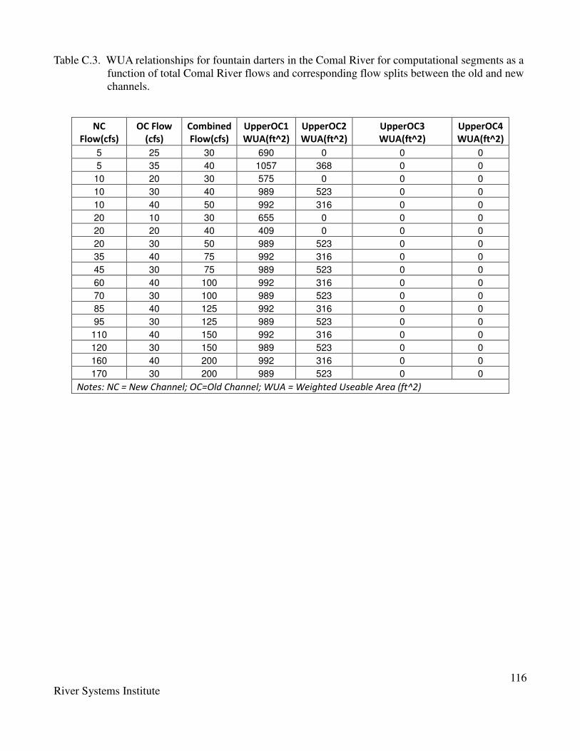
116
River Systems Institute
Table C.3. WUA relationships for fountain darters in the Comal River for computational segments as a
function of total Comal River flows and corresponding flow splits between the old and new
channels.
NC
Flow(cfs)
OC Flow
(cfs)
Combined
Flow(cfs)
UpperOC1
WUA(ft^2)
UpperOC2
WUA(ft^2)
UpperOC3
WUA(ft^2)
UpperOC4
WUA(ft^2)
5 25 30 690 0 0 0
5 35 40 1057 368 0 0
10 20 30 575 0 0 0
10 30 40 989 523 0 0
10 40 50 992 316 0 0
20 10 30 655 0 0 0
20 20 40 409 0 0 0
20 30 50 989 523 0 0
35 40 75 992 316 0 0
45 30 75 989 523 0 0
60 40 100 992 316 0 0
70 30 100 989 523 0 0
85 40 125 992 316 0 0
95 30 125 989 523 0 0
110 40 150 992 316 0 0
120 30 150 989 523 0 0
160 40 200 992 316 0 0
170 30 200 989 523 0 0
Notes: NC = New Channel; OC=Old Channel; WUA = Weighted Useable Area (ft^2)

117
River Systems Institute
Table C.4. WUA relationships for fountain darters in the Comal River for computational segments as a
function of total Comal River flows and corresponding flow splits between the old and new
channels.
NC
Flow(cfs)
OC Flow
(cfs)
Combined
Flow(cfs)
BottomOC1
WUA(ft^2) BottomOC2 WUA(ft^2)
5 25 30 0 5755
5 35 40 10830 5588
10 20 30 0 5688
10 30 40 0 5662
10 40 50 10820 5520
20 10 30 0 5847
20 20 40 0 5662
20 30 50 0 5662
35 40 75 10820 5520
45 30 75 0 5662
60 40 100 10820 5520
70 30 100 0 5662
85 40 125 10820 5520
95 30 125 0 5662
110 40 150 10820 5520
120 30 150 0 5662
160 40 200 10820 5520
170 30 200 0 5662
Notes: NC = New Channel; OC=Old Channel; WUA = Weighted Useable Area (ft^2)

118
River Systems Institute
Table C.5. WUA relationships for fountain darters in the Comal River for computational segments as a
function of total Comal River flows and corresponding flow splits between the old and new
channels.
NC
Flow(cfs)
OC Flow
(cfs)
Combined
Flow(cfs)
Above
Clemens
WUA(ft^2)
Above
VNotch
WUA(ft^2)
Above Guad
WUA(ft^2)
5 25 30 0 0 0
5 35 40 0 0 0
10 20 30 0 0 0
10 30 40 0 0 0
10 40 50 0 0 0
20 10 30 0 0 14150
20 20 40 0 0 9851
20 30 50 0 0 9851
35 40 75 0 0 8543
45 30 75 0 0 8543
60 40 100 0 2126 3440
70 30 100 1965 2126 3440
85 40 125 1995 1473 2028
95 30 125 1995 1473 2028
110 40 150 2499 896 1273
120 30 150 2044 896 1273
160 40 200 2000 383 673
170 30 200 2000 572 882
Notes: NC = New Channel; OC=Old Channel; WUA = Weighted Useable Area (ft^2)

119
River Systems Institute
Appendix D
Depth, Velocity, and Combined Suitability Contours for Texas Wild Rice and Fountain Darter in the San Marcos River for Simulated Discharges
(by electronic download)

120
River Systems Institute
Appendix E
Comment response matrix for Draft Report
Commenter Comment Response Myron Hess Page 43: I found the last
paragraph regarding the Comal Springs Riffle Beetle to be a bit difficult to follow. Would it be possible to expand a bit on the rationale for using surface area of flow in modeling and, specifically, how that relates to the recolonization aspect?
Text was updated and clarified on the rationale used for surface area modeling and includes more discussion on recolonization.
Page 43: In the last sentence of this paragraph, should "but" be "by"?
Fixed.
Page 43: Also, the basis for the use of the 0.02 foot depth is unclear. The previous discussion seems to suggest that 1 inch is the usual minimum depth. Further explanation would be appreciated.
Text was clarified to address the 0.02 foot criteria as this is the threshold depth for wetting and drying in the solution of the hydrodynamic model and therefore the accuracy limit on depths for this application.
Page 45: Figure 26, although labeled as depth habitat suitability, appears to be a duplicate of Figure 27 and a depiction of the velocity habitat suitability curve.
Updated the correct Figure.
Page 57: I found the last paragraph in the Dissolved Oxygen section to be a bit difficult to follow. Would it be possible to expand a bit on the discussion of the diel DO swings? In particular, it is unclear if the observed field values of DO include 24-hour monitoring. At any rate, some expanded discussion, if possible, of the diel swings would be helpful
Expanded the discussion on implications of diel oxygen swings. See page 41 where it states that the diel model calibration and validation runs were based on measured hourly data sets.

121
River Systems Institute
Page 57: Also, the discussion here seems to suggest that night-time DO levels likely would not be limiting at low flows. However, discussion elsewhere in the document, e.g. p. 67, seems to suggest that night-time DO levels could be problematic for some species. Some further clarification would be helpful.
This section was clarified to explain that the diel swings in DO under existing vegetation and flow conditions are not anticipated to be limiting. Also added discussion that with low flows and potential vegetation die-off’s that night time DO levels may become problematic.
Page 81: The references, on this page, to Figures 52-54 are, apparently, all off by one Figure. That is, it appears that the reference to Figure 52 should be a reference to Figure 53, etc.
Fixed figure reference sequence.
Jackie Poole Hard copy edits to the report were provided.
All editorial comments were made as suggested. Clarifications were also made were suggested edits were related to unclear material presentation.
p. 22, paragraph 2 - Hydrodynamic Modeling - Physical Characterization - While the 1998 flood did deposit some material above University Drive bridge, most of the material came from construction sediment from Sessoms Creek.
Revised to text to note the contribution of sediment was primarily from Sessoms Creek construction sources.
p. 32, Table 4 - Why wasn't wild-rice included in the vegetation class and roughness assignments?
All of the data were collected from the Comal River and therefore no wild rice stands were measured. At the time that the work on the San Marcos was undertaken, the USFWS asked that we not disturb wild rice stands so no data was collected. Roughness was assigned however based on other codes. Text clarified in this regard.
p. 45, Fig. 26 - Graph should be the depth HSI curve.
Fixed.
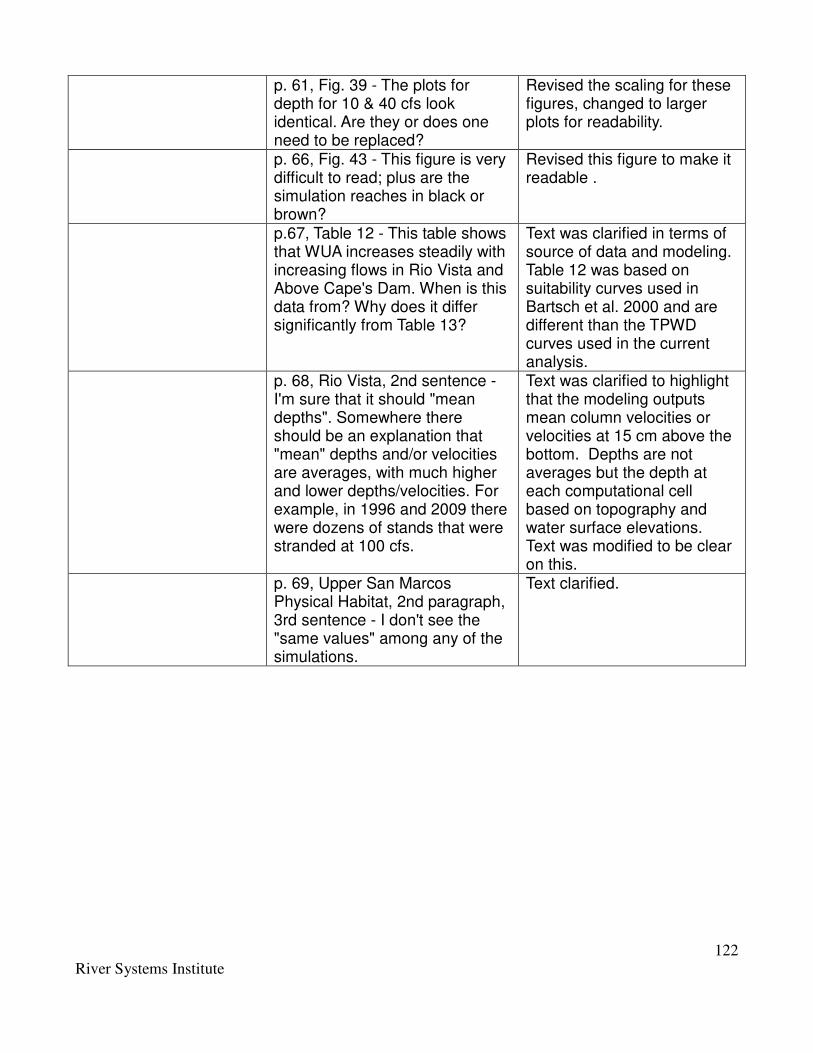
122
River Systems Institute
p. 61, Fig. 39 - The plots for depth for 10 & 40 cfs look identical. Are they or does one need to be replaced?
Revised the scaling for these figures, changed to larger plots for readability.
p. 66, Fig. 43 - This figure is very difficult to read; plus are the simulation reaches in black or brown?
Revised this figure to make it readable .
p.67, Table 12 - This table shows that WUA increases steadily with increasing flows in Rio Vista and Above Cape's Dam. When is this data from? Why does it differ significantly from Table 13?
Text was clarified in terms of source of data and modeling. Table 12 was based on suitability curves used in Bartsch et al. 2000 and are different than the TPWD curves used in the current analysis.
p. 68, Rio Vista, 2nd sentence - I'm sure that it should "mean depths". Somewhere there should be an explanation that "mean" depths and/or velocities are averages, with much higher and lower depths/velocities. For example, in 1996 and 2009 there were dozens of stands that were stranded at 100 cfs.
Text was clarified to highlight that the modeling outputs mean column velocities or velocities at 15 cm above the bottom. Depths are not averages but the depth at each computational cell based on topography and water surface elevations. Text was modified to be clear on this.
p. 69, Upper San Marcos Physical Habitat, 2nd paragraph, 3rd sentence - I don't see the "same values" among any of the simulations.
Text clarified.

123
River Systems Institute
p. 70, Table 13 - What units are the WUA in? What is the 2009 analysis based on? There's not an explanation that I can see. The 2009 numbers are problematic. All show a break point at 65 cfs. WUA show shouldn't peak at 65 cfs if observations show that depths are unsuitable (i.e., plants stranded) at 100 cfs. There are similar issues with the fountain darter Table 15.
Units were added and text clarified as to the source data used in the modeling. Do not confuse the estimated total habitat for wild rice or fountain darters versus specific locations where stands may have been dewatered while other areas are predicted to be suitable although not occupied. Text was added to address this issue and clarify interpretation of modeling results.
p. 88, Suckermouth catfish - Suckermouth catfish would also affect Texas wild-rice directly through herbivory and indirectly through downed trees that could scrape wild-rice off the river bottom during floods.
Text was added to note this potential impact from catfish and the potential for impacts associated with physical disturbance of tree movement during flooding.
Calvin Finch/San Antonio Water System
On May 15, 2009, SAWS submitted comments on the Influence Diagrams that are an important component of this study. Other EARIP stakeholders also submitted comments. In keeping with the procedures utilized to date with other Science Subcommittee reports, an appendix should be developed that catalogs this feedback. This appendix should also be referenced in the report on page 11 (Executive Summary) and page 15 (Influence Diagrams for Target Species). The final report would be further strengthened by an explanation as to whether and how the comments received were incorporated into the analysis.
These diagrams were primarily developed to support the USFWS HCP analysis and ancillary to the work reported in this document. However, an appendix was added to highlight comments received. Reference to the added appendix was inserted as requested. Text was added to the report to clarify this issue.

124
River Systems Institute
Additionally, describe how the influence diagrams touch upon the various aspects of the model results. For example, what aspects of the model could management strategy proposals, such as ecological restoration activities being considered by other EARlP subcommittees, improve upon? Also, how would those improvements be reflected in the outputs of the model?
Text was added to highlight where the modeling in this report ‘fit into’ the influence diagrams although the figures do in fact explicitly show where these data/results fit! A small section was added to the report that highlights how the revised data and modeling could be used to support these analyses under the HCP but are beyond the scope of this report.
In general, a section of the report should be developed that states the appropriate uses of the biological flow model. What can the stakeholders ask the model to simulate, and what kinds of scenarios can the model not accommodate? A local example can be found in the Edwards Aquifer MOD-FLOW model, where the appropriate usage of the model (i.e. regional management strategies) is contrasted with unsuitable uses of the model (i.e. molecules of contaminant movement or transport). A similar format in the report will be undoubtedly helpful as the stakeholders and Steering Committee work towards identification of actions, alternatives, management, etc.
This is really a HCP level question and not a J charge report question. As noted in the previous response, text was added to highlight how the revised data/modeling can be used to answer specific types of scenarios.
In the Introduction paragraph on page 12, an extraneous word ("and") is inserted into the name of the process (Edwards Aquifer Recovery and Implementation Program). SAWS would recommend deletion of the extraneous word.
Fixed throughout the document.

125
River Systems Institute
Figure 1 on page 13 is mislabeled as a map of the San Marcos system, but the map is of the Comal system. A notation in the text indicates that Figure 1 will be updated to reflect the style in Figure 2. During this update process, the caption label should be corrected.
Fixed.
On pages 16 and 19, the report states that additional components to the influence diagram will need to developed to evaluate the effects of possible HCP actions on Comal Springs riffle-beetle, Texas Wild-rice, and Fountain Darers. Would the authors undertake this process of expanding upon the initial Influence Diagrams, or would the process of expanding upon the Influence Diagrams include all interested EARlP stakeholders?
This would be undertaken as part of the HCP process as the USFWS works on issues related to the BiOp. I will be part of this process as can the stakeholders.
The portion of the report that focuses on "Development of Computational Meshes" on page 23 discusses examples of varied interpolation algorithms or gridding procedures to create the Most Representative Surface (MRS). Was the same interpolation method used in both river systems? Did each of the river segments evaluated in both systems use the same interpolation algorithms, or were there differences between systems and within each system between reaches? A notation is given in the last sentence for finding the details of the methods used; however, an expanded, yet still generalized, discussion of the type(s) of gridding procedures by system and by reach might be helpful.
The same gridding algorithm (natural neighbor) was used for both systems and all sections. This has been added to the text for clarification.

126
River Systems Institute
Page 24 discusses the use of two-dimensional hydraulic models, such as Surface-Water Modeling System (SWMS or SMS), RM2, and HEC-RAS, to derive water surface elevation and flow velocity. The draft report could be enhanced if a general introductory paragraph was developed where an examination of the available scientific literature were to be undertaken to determine the strengths and limitations of these various models and the suitable versus unsuitable application environments the models may or may not be applied within.
Text was added the highlights the appropriateness of the hydrodynamic models used. These models are in common use for this class of modeling in applied river studies and references to document this have been added. Since this is relying on a ‘legacy model development and application’ it will be more appropriate to include this material when the updated models are used in the new work currently underway.
127
River Systems Institute
The last paragraph on page 24 describes cross-section calibration to match observed water-surface elevation-discharge data through the manipulation of the cross-section's Maning's n-value within HEC-RAS. In simplified verbiage, the cross-section was made more or less "rough" until the water level in the model matched water level observations. Is the manipulation of Maning's n-value an accepted technique in river modeling? Might other characteristics of the model profile be manipulated to match observed water levels, such as cross-sectional profile, depth, or shape? The concern here is that roughness coefficient manipulation has an impact on modeled velocities. Velocity of flow is an important component of the habitat references of the sentinel species, such as fountain darer (slow but not stagnant), wild-rice (quicker up to a point), and riffle-beetle (fast enough to facilitate gaseous diffusion across the air 'bubble' the beetle breathes from). The final report would be strengthened if a section was developed that addresses whether or not, and how much, the manipulation of Maning's n-value impact the suitability of habitat in that cross-section.
This is the standard accepted approach to calibrate one-dimensional hydraulic models used to predict water surface elevations. Modification of measured topography is not an acceptable practice! The HEC-RAS model was only used to estimate the water surface elevation versus flow relationships used in the 2-dimensional model where the velocities are predicted. HEC-RAS was never used to simulate velocities. Text was modified to make this clear. This is not necessary as Manning’s n only applies to estimate the stage-discharge boundary conditions for the 2-dimensioanl model and therefore has absolutely no impact on suitability of fountain darter or wild rice habitat!

128
River Systems Institute
On page 27, an assumed ratio of partition of flow rates (3:2:1) between large, moderately-large, and medium springs (respectively) was used. A similar procedure is described on page 28, where more than 200 springs at San Marcos were simplified into eighteen or twenty-one spring inputs. Providing a discussion of any other ratios examined would be helpful, and what were the possible effects of varying this assumption? This kind of an examination would be analogous to a simplified sensitivity analysis to determine the influence of where and at what proportion (ratio) the influence of smaller springs and seeps have on the system relative to large and medium springs. This is thought to be especially important in riffle-beetle habitat.
No other ratios were examined. I provided a spreadsheet to the RIP early on and requested review and comment. None were ever provided. This is however, something that will need to be addressed/reviewed for use in the revised modeling currently underway.
Landa Lake is misspelled on page 27 in the ninth line on the page.
Fixed.
The last sentence of the first paragraph on page 27 discusses interpolation of data for 'other discharges' simulated in the report. Please elaborate on the flow data that forms the basis of this section, and on the methods or techniques used to interpolate. This sort of a discourse is important as the Science Subcommittee, Steering Committee, and stakeholders will be using this tool developed by Dr. Hardy et al. for support of decision-making concerning flow levels that have not been formally studied.
Text was clarified to indicate a simple linear interpolation of values was used for specific spring flow discharges from the data in Table 1. The flow data is presented in Table 1 and as the text indicates, the origins of these data are Brune 1981 for spring flow rates. Flow splits are simply what were modeled to examine potential implications of different flow volumes split between the old and new channels.

129
River Systems Institute
In the third paragraph on Page 28, an addition of 5 cfs to the slough area of Spring Lake was simulated in the 2-D hydraulic model to account for 'golf-course runoff through the area. What is the source of the golf-course runoff (i.e. municipal water, well water, surface water, etc.) and what is the literature or regulatory source for the 5 cfs number?
The 5 cfs was taken from our synoptic flow measurements during the original fieldwork. Text was clarified to indicate this and was intended to account for all unmeasured sources contributing to this section of the lake.
The first paragraph on Page 29 discusses interpolation of flow values at other discharges for the San Marcos system. Please apply Comment #12 above to this section also. It will be helpful to the decision-making process for stakeholders and decision-makers to have an understanding of the assumptions, which form the basis of the interpolations, which in the end result in the outputs of the flow model.
See response to previous comment.
The scaling of wastewater treatment plant discharge cures discussed on page 29 would seem appropriate for standard municipal wastewater discharges, such as from the City of San Marcos wastewater treatment plant. Does discharge from the A.E. Woods state fish hatchery mimic the same pattern as the City wastewater plant? It would seem that these two facilities might have differing operational patterns - does the Tchobanoglous (1991) citation include different curves for different types of facilities, or was the same curve used, and what is the effect of this assumption and scaling on habitat in affected downstream reaches?
At the time of the original study there was not available data for the A.E. Woods hatchery. This is something that needs to be addressed in the revised modeling currently being undertaken in support of the HCP. The citation was used based on our evaluation as the most reprehensive for this type of facility. There is no implication of this assumption on scaling of habitat in downstream reaches. It only affected the simulation of temperature and dissolved oxygen or the addition of incremental flow accretions.

130
River Systems Institute
On page 31, why was Texas Wild-rice excluded from other vegetation species that were assigned roughness values based on vegetation/vertical velocity profile data? Is this omission due to the data being collected from the Comal River, where Texas Wild-rice is not found? It would seem that omitting roughness values for Texas Wild-rice would impact the results of suitable habitat to some degree. Wild-rice is known to prefer a certain range of velocities, as do fountain darers. Is there a potential to exclude segments of suitable habitat for these species based on the omission of Texas Wild-rice roughness values?
All of the data were collected from the Comal River and therefore no wild rice stands were measured. At the time that the work on the San Marcos was undertaken, the UWFWS asked that we not disturb wild rice stands so no data was collected. Roughness for wild rice was not omitted but assigned roughness from similar plant forms where data was available. There is no potential to exclude segments of suitable habitat due to omission of roughness values since roughness was in fact assigned for wild rice!

131
River Systems Institute
Table 4 on page 32 indicates two vegetation classes where the lack of vertical velocity distribution caused the assignment of generic roughness values. Aquatic plant pictures found in various locales online show two vegetation classes with very different morphologies and different growth environments. Riccia thatans seems to be a submerged low-profile aquatic plant, while Justicia Americana appears to be grown more emergent and with a larger vertical profile. Insertion of a sentence or two that describes the percentage of the study area affected by these generic roughness values would be helpful, including a discussion of possible suitable habitat within that percentage of the study area that is impacted by this generic roughness value. It is reasonable to assume this impact would be relatively small, though examination of this aspect would be beneficial.
Text added as requested. This will be addressed in the revised modeling using the updated vegetation polygon mapping.
On page 32 in the first paragraph of the "Vegetation Mapping" section, Texas State University's former moniker (Southwest) is used.
Fixed.

132
River Systems Institute
The top of page 34 discusses the simulation of water temperature over a 48-hour period associated with the hottest meteorological conditions as a worst-case scenario. SAWS understands the value of having these snapshots" of habitat temperature at different flow levels, though is concerned about the usage of the snapshot over long-term conditions in the habitat. The report examines available scientific studies on the reproduction and various life-stages of fountain darers on page 47. Later, on pages 52, 54, 55, 59, 65, 79, 80, and others, temperature is singled out as the limiting factor or part of a suite of limiting factors for various reaches of the habitat in both the Comal and San Marcos systems. It is difficult to understand how a 48-hour temperature can be 'stretched' out over longer durations of time such that it impacts fountain darter reproduction. How could a duration of 48-hours of high temperatures be sustained over days, months, or a year such that it results in the loss of multiple cohorts of breeding fountain darters, thus threatening the species' survival and recovery in the wild?
The modeling in this manner was undertaken in the original study explicitly at the request of the USFWS and no new water quality simulations were undertaken for this report (out of scope). This will be addressed with the revised water quality modeling currently underway to support the HCP. This is simply a very conservative approach that offers the maximum protection for the species. I agree to some extent. More refined simulations need to be undertaken as part of the revised water quality modeling efforts.
133
River Systems Institute
This kind of an assumption in the study is an important issue that scientists and stakeholders will have to examine. While short-term temperatures may exceed a threshold of fountain darer preference for a given time-frame, it is unlikely that those temperatures will be sustained for periods or lengths of time that affect the survival of the darer. Impacts from temperature on eggs laid or larvae developing in those time periods have been demonstrated, but it is a tenuous stretch to state that temperature becomes a limiting factor in habitat over the long term and it is not entirely valid to limit a habitat solely on temperature modeling outputs generalized from a short-term duration to a long-term duration.
This should be addressed during the revised modeling where time series of flow regimes should be used to reflect the duration of conditions rather than the snap-shot index day used previously. This will allow a much better assessment of potential temperature induced bottlenecks if they in fact exist under different low flow sequences during any period of the year.
Short-term deleterious temperatures should not mean an entire portion of habitat is unusable or that species reproduction is irreparably harmed. It is unclear how the model can take an instantaneous temperature that persists long enough to adversely impact darter habitat over an extended time scale based on a short time scale sample of temperature data.
See previous comment.

134
River Systems Institute
On page 37, water quality model calibration is discussed, including the adjustments necessary to wind speed and cloud cover. Was there a scientifically based rationale for adjusting solely those factors, or are there other factors such as local runoff, mixing within the water column, canopy cover, etc. that might have been adjusted? Why were these factors selected over others, and what was the discrepancy between the model and the observational data? Was the model systematically too war or too cool, and how was the adjustment handled (i.e. more or less wind, more or less clouds)?
This is the accepted method for calibration of water temperature models. We had no data of these types and not sure they exist even now. This is clearly illustrated in the predicted versus observed simulation results provided in the report. The model over and under estimated the temperature depending on location and time and but was within accepted calibration limits. This is obviously something that will be documented and discussed in the revised modeling.
On page 37, dissolved oxygen (DO) was modeled without considering a number of other chemical and biological processes. Do the authors have an estimate, based on their experience or knowledge of other systems and other work, of the DO demand from these processes that were not considered?
This is because the requisite data for this was not available. We considered the fact that the observed versus predicted DO from the data collected during or studies to have been sufficiently close and therefore these were not a primary concern.
It is stated that calibration of DO on page 37 relies heavily on the use of dam reaeration. This would seem to indicate that the modeled DO was lower than the actual DO measurements. Is this the case, and if so, are there any explanations as to why this might be occurring? Does the model under-contribute DO from phytoplantonic algae and other macrophytes, or is there another possible source?
No. It is simply that this parameter in conjunction with the physical setting of the various dam structures was practical and defensible for model calibration. The simulation results compared to observed data clearly shows acceptable calibration and validation of model results.
135
River Systems Institute
Page 38 discusses division of the San Marcos River into twenty-one sections based on in-reach similarities. In what aspect were these similarities based that resulted in the division into like segments (i.e. vegetation, substrate, depth, etc.)?
The primary factor was computational efficiency and physical characteristics (i.e., backwater reaches immediately above dams, reaches below dams, and the factors listed in the comment.
A citation is needed on page 42 at the end of first paragraph of the "Habitat Suitability Cures" for the annual wild-rice monitoring data.
Added.
A citation is needed on page 43 in the third and fifth paragraphs describing the genetic analysis that suggests a riffle-beetle “population genetic bottleneck" and "recolonization" of previously dry spring runs. A similar citation is needed on page 59 discussing a shift in the genetics of the riffle-beetles in spring run 1.
Added.
In Table 9 on page 46, are the Suitability Indexes for Texas Wild-rice the same (0.04) between 5.30 feet of depth and 9.0 feet of depth?
Yes.
In the last paragraph of page 47 there is a discussion that the expert technical team "felt that use of vegetation type was sufficient.." and so excluded vegetation height from the habitat modeling. Explanation or elaboration as to why this approach was chosen would be appreciated in the final report.
As noted in the text, vegetation height is not available for either the Comal or San Marcos River systems so could not be included in the analysis.

136
River Systems Institute
On page 50 in the section on "Physical Habitat Modeling" an assumption was used that vegetation and substrate characteristics would be unchanged due to fluctuations in simulated flow rate. Over what time scales would this assumption be valid, and on what time frame do vegetation changes begin to occur based on available observational and monitoring data to date?
This is simply the assumption necessary at the time of the original studies were collected (basically one set of vegetation maps existed!). Updated modeling to support the HCP can utilize changes in vegetation coverage and composition and should be discussed during the revised modeling and potentially in light of either restoration actions or changes in vegetation due to sustained low flows.
On page 51, the Comal Springs riffle-beetle habitat equation does not include substrate. However, on page 43, riffle-beetles are stated as preferring gravel substrates. This binary habitat equation is characterized as "the most germane way" of representing habitat. It seems that a binary approach is overly simplistic and may under-estimate or over-estimate habitat given the previous section's statement on beetle substrate preference.
We felt that since the beetle has been empirically demonstrated ‘to recover’ from complete spring run dewatering, the role of substrate was not as important relative to maintaining surface flows. This is a bit simplistic but is conservative in terms of preserving potential habitat areas as long as one maintains surface flows. This can be revisited under the revised modeling current underway.
On page 51, interpolation from the habitat suitability relationship to each node is discussed. What was the interpolation method or technique used?
The associated depth or velocity value at the node is used to interpolate the associated suitability value for the habitat suitability graphs using linear interpolation. Text added to clarify this.

137
River Systems Institute
The section entitled "Fountain Darter: System-Wide Physical Habitat Using Mean Daily Temperatures" on page 59 states that the primary reason for habitat decline under lower flow rates was temperature. It is unclear why temperature is a limiting factor for fountain darers, especially since the timeframe of the temperature occurrence is artificially stretched in duration in the model.
This statement is consistent based on the modeling assumptions used where maximum daily temperatures limit habitat from a decreased reproductive perspective. As noted in previous responses to comments on the temperature issues, more refined analyses are anticipated using the revised models currently being developed.
In figure 39 on page 61, the color-ramp "keys" are difficult to read. Are the colors in each contour plot of the Upper Old Chanel (Comal) similar between plots, or do the values for each color change between plots?
Graphs have been clarified.
On page 74, there is a statement that flows below 65 cfs cause stands of Texas wild-rice to be proportionally more vulnerable to physical disturbance from recreation. In the qualitative evaluation, were the Weighted Usable Areas (WUAs) adjusted based on this evaluation? If so, by what amount?
No adjustments in WUA were ever made based on this or other qualitative evaluations.

138
River Systems Institute
In general, it seems that the model focuses on riverine habitats. Monitoring by BIO-WEST on behalf of the Edwards Aquifer Authority (EAA) indicates that a relatively small portion of the fountain-darter population is found in the rivers. The lakes provide space the most abundant populations and highest quality habitats in the system. How does this report incorporate the lakes as important habitat with quality WUAs? Also, the stakeholders may benefit if context is provided between the WUAs identified in this draft report compared to previous work in these systems.
Both Landa Lake and Spring Lake were modeled for fountain darter habitat. No specific focus was given to only riverine habitats. As noted, both lakes systems were modeled and included in the habitat summary analysis. The report does in fact report on habitat modeling from the previous studies for each system!
On page 91, provide a citation for the increased infection rates by gill parasites on San Marcos darters.
Added.
Glen Longley Editorial comments provided in report electronically.
All suggested editorial comments were made in the report.
Ed Oborny Acknowledgements - Oborny not Orborny
Sorry Ed!
Page 11 - Executive Summary - Paragraph 1: scientific names switched for fountain darter and riffle beetle.
Fixed.
Page 11 - Paragraph 3: As written this paragraph is very misleading. It claims data collected through 2009 was used and models were updated, when in fact a lot of the information used for the modeling was the same as the original and in many cases the old modeling was not updated at all, and results were the same as originally reported. This needs to be clear throughout the report.
This has been clarified to indicate what was updated and what was used from previous work throughout the report as requested.

139
River Systems Institute
Page 12 - last paragraph - Why not use BW spring flow data from 2003 through 2008. 13 times measurements were made over this period. Min. 22.9% Median 23.8% and Max. 30%. The use of old data happens repeatedly in this report when much newer information is available.
We updated to use your numbers, although there is in fact very little difference between the two sets of numbers and likely the differences are well within measurement error.
Page 12 - last paragraph - “Old channel only holds 40cfs”. This was before the installation of the new culvert system. Can easily handle 100 cfs now.
Modified the text to clarify this change in capacity.
Page 12 - last paragraph - “…3.2 miles long…, …another 2km…” - consistent units.
Revised to report to use all English units.
Page 14 - Figure 2 - Scale way off.
Fixed.
Figures 4, 5, 6, & 7 - Riffle beetle section - All your pictures are of the Comal Springs Dryoptid beetle.
Fixed and thanks for the photos!
Figure 6 - No Comal Springs riffle beetles have ever been found at your picture of Spring run 5 at Comal.
Updated with the picture you sent.
No real discussion of the influence diagrams or summary paragraph to say what they were or will be used for. See next point.
Text was added to clarify the purpose of the diagrams, what their intent is, and how the modeling ‘connects’ to them.

140
River Systems Institute
No transition from Influence diagrams to Hydrodynamic modeling. Need some text to make this smoother. If there is no transition, you need to set up this section better with the why this is being done. What it is going to be used for. What are the advantages and limitations. The entire section needs to cover either in summary format upfront, or in each individual component moving through the report. Start with what was originally done, what was discussed among the group as needing revision, what was actually revised, and what is still to be done.
A transition was added as suggested. See previous comment.
Page 22 - Physical Characterization section: You talk about 1998 flood, failure of Capes dam in 1999, and conclude with you are using the channel topographies collected during 1991? Assuming you mean 2001?
Fixed dates and clarified text throughout the report.
The physical characterization section would also be a good section to talk about all the sedimentation that has occurred in Sewell Park and City Park since the 1998 flood, cite the work done by Texas State (Curran, Engel and others), and discuss how this might affect modeling results.
Added text to highlight the sedimentation accumulations, and potential effects.
SWMS and SMS the same - consistency needed
Model nomenclature has been made consistent throughout the report.

141
River Systems Institute
Page 25 - Comal river - spring nodes? Was any of this updated based on work conducted the past 10 years (springflow augmentation, dye tracer studies, etc. ) by the Edwards Aquifer Authority? Might be good just to mention some of this work and the possibility of it’s inclusion in the next round.
Text was added to indicate that this data was derived from the reference sources, new work is now available, and will be incorporated into the updated modeling currently underway. A spreadsheet of these assumed flow contributions was in fact provided to the RIP for comment but none were ever provided.
Page 28 - San Marcos river - FESWMS Paragraph 1, RMA-2 Paragraph 2
Clarified.
Page 29 - Unclear as to whether current day City of San Marcos WWTP information was used or the original information.
No new water quality modeling was undertaken. Text clarified throughout to highlight this fact.
Page 31 - VEG Dependent Hydraulic Roughness section - veg maps available for both systems? Were the original vegetation maps used in the updated models? What were the dates of the maps used?
Vegetation maps were available for both systems but only hydraulic roughness data was collected from the Comal. Dates and sources of maps were added to the report and clarified that these maps were used in all simulations.
Page 32 - Veg mapping section - I recommend moving this section ahead of the VEG Dependant section to avoid the questions I just asked above. Who mapped the Comal? You say Roland Roberts and David Lemke in sentence 1, then Jonathan Beale on the next page.
Moved as suggested. Added clarification of sources as noted in responses above.

142
River Systems Institute
Page 37 - Comal River WQ modeling. Was any new water quality modeling done at Comal? Or does this report just discuss what was presented in the original report? Was any of the intensive temperature information being collected throughout the Comal River via the EAA Variable Flow Study over the past 9 years used to validate these model results? If not why? Seems like this data should at least be mentioned?
No new water quality modeling was undertaken and text added where appropriate to clarify this. No. Text was added to indicate the availability of these data and that it is being used in the revised modeling for both river systems.
Same question as above for the San Marcos WQ modeling?
Same response as above!
Page 42 - Habitat Suitability Curves - First sentence - What data and how was it used to update? This needs to be explained to the reader. This is especially critical considering the major change in results for Fountain darter habitat at SM shown later in the document.
Clarified.
Page 43 - ComalSprings Riffle beetle. 4th sentence is not accurate, although this is what was thought in 1998. They also occur in upwelling areas in Landa lake. Paragraph 3 needs a major update. Need a description of the range expansion study done back in 2002. Also need to discuss that they have recently been found at several locations with a number of individuals in Spring Lake. Paragraph 3 - need to reference your genetic statement.
Obtained an updated map from USFWS that show known locations and updated the text based on this map. Updated the text to reflect this updated material as requested. Added.

143
River Systems Institute
Maybe a description is upcoming, but Randy Gibson has delineated a map of CSRB area in all three spring runs and that should be used in the assessment. Also, although a consensus was reached for surface modeling, it was only because it was the easiest thing to do with the time available. In my mind, there was always the assumption that this would be explained in this report. This being the fact that the CSRB is found throughout the lake, and that the spring runs only make up a portion of the habitat, etc. etc. However, modeling this area will provide some indication of potential impacts. Also the discussion on subsurface habitat needs to happen here. Just because an effect is shown at the surface for this species does not necessarily mean that the population is at risk because they simply may go subsurface.
Has been included. Updated the text to reflect this modeling approach and that refined modeling with the updated modeling efforts will revisit the approach taken. Agree. And added text to point this out.
Figure 26 and 27 are the same - just the velocity plot.
Fixed.
Page 47 - 4 or 5 degree F buffer. Struggling with the math here.
Clarified text.
Figure 28 - being that fountain darters are found throughout Landa Lake at depths to 10 feet and in Spring Lake at depths exceeding 20 ft, this curve needs to be explained. Either some discussion that only riverine habitat is being modeled (true at San Marcos but not at Comal) so I am not sure how best to explain this. Thoughts?
HSI was modified to show no reduction in suitability for depths and the models rerun with this updated HSI.

144
River Systems Institute
Figure 30 - What information was used to generate this figure. It does not match at all with the last 9 years of EAA data. Was the EAA data actually used at all? Or was it just reviewed to see if stuff was in the ball park. An explanation of how that data was used or not used needs to be presented.
The original vegetation HSI was used for all the simulations runs due to incapability of the vegetation coding used in the original vegetation mapping for both systems and text was added to document this issue, which will be addressed in the revised modeling based on the updated vegetation mapping for both systems.
Page 52 - Comal Temperature. Figure numbering wrong. Need to define “upper critical thermal range” As presented here one would think the old channel would be a barren wasteland at 78 F, rather than just a channel with summertime temperatures that it sees pretty much every year in which some larval success would be reduced. Wording is way too suggestive here. Just needs to be defined and described for what it is. Also need to discuss in the text that this means only 10cfs and 5cfs would be flowing through the old channel at 60 cfs and 30 cfs respectively. This is an extremely important point.
Fixed. Text was added to clarify how this ‘concept’ was applied and a better explanation of the practical implications. Text was added to clarify this.
Need to pick 80 F or 78 F, jump back and forth through section.
Standardized the temperature used.
Page 55 - please provide a reference for the USGS diel DO study in Landa Lake.
Personal observation of them doing it! I found the spreadsheet of their data but have no idea now who did it!
Page 57 - CSRB section - What is this sampling discussion. There is so much more recent and better data here. I am not sure what sampling you are even talking about.
This is data we collected during our original study on Comal. I do not agree that the newer data is necessarily better!

145
River Systems Institute
Figure 36 - Is this all Spring run area, or the area the Randy Gibson provided as known CSRB habitat in these springs?
All spring run area only. Text added to clarify this.
Page 59 - I’m Confused. The comal section shows WUA with temperature included for a number of flow scenarios. Then moves to the San Marcos section that just talks about mean daily temperature and shows one figure of temp but no WUAs presented in this section. Then moves directly to Texas wild rice. Then to SM WUA.
Reorganized the text to keep systems together. Cut and paste error on moving things around!
Somewhere need to state that although new HSI criteria were generated, no new modeling was done at Comal for the fountain darter. This might be important because of the major change the new criteria caused in overall WUA results in the SM.
New modeling was in fact done in Comal for fountain darters based on the updated habitat suitability curves.
Page 59 - last paragraph - 2nd to last sentence. Please describe what you mean by “unacceptable levels”. Isn’t this simply “area with less suitable conditions for larval survival”? Need to formally define “unacceptable” and then state over what time period this might be unacceptable, etc. Using that term requires more explanation. Might consider simply calling it what it is and avoiding that term.
Text was clarified to use your suggested language as it better reflects what is actually being presented.

146
River Systems Institute
Page 60 - figure 37. The legend states “unsuitable temperatures for fountain darters”. Again, these temperatures are fine for darters to survive, and even reproduce at some level. It does cause lower success rates of larval survival based on laboratory studies, but does not mean that darters could not reproduce successfully in Landa lake and move back into these areas for feeding, living, etc. Again a better description of what is meant here needs to take place in the text.
Clarified the associated text to reflect what it is intended to illustrate.
Page 61 - can’t read legends at all in Figure 39
Added text to clarify the legends.
Page 62 - Figure 40. Again can’t read legends, but assuming blue is 1.0, the figures appear to be flipped, unless I am missing something. I would anticipate better habitat conditions at 40 cfs than at 10 cfs, which is not what the figure is saying. Looking at the supporting text, it appears my assumption is wrong. Regardless, the maximum combined suitability values on the figure don’t match with their respective examples. (Probably flipped).
Fixed and added text to better describe to the reader what the results mean. Figures were not reversed.
Page 63 - Table 11 formatting needed
Fixed.
Page 70 - 2nd full paragraph. Can you include a table of the comparison that you describe here. I am unclear what was actually done. Does not seem to jive with what Jackie has been telling me about how far off the model is relative to occupied areas. What am I missing?
Figures were in fact mislabeled and were simply the frequency of predicted suitability values for all modeled cells. The correct histograms showing the frequency of suitability of occupied rice cells have been updated.

147
River Systems Institute
Page 73 - 1st paragraph - the word “occupied” simply means model predicted, correct? It is not what Jackie would call occupied? - which means really there, correct?
Occupied means a wild rice plant was at that location compared to the model predicted suitability at that location.
Page 78 on - Fountain Darter SM - The bulk of the discussion (text) is on the old results. However, the new HSI criteria causes such a drastic change in the overall results that it would be good to have a discussion on why this is and which you feel is more appropriate, etc. This will influence whether or not to even use Figure 52, which is completely misleading if you feel the update HSI information is valid.
Text added to discuss changes in the relationships (and why) as well as having added text on use of the various simulation results.
Page 83 - last paragraph - Sentence 3, “However, it is clear regardless…………….rapid declines……….below about 65 cfs”. I contend this is no more true than rapid declines occur from 65 cfs to 100 cfs - see Figure 51 Total 2009 if one considers the updated HSI info. Again highlighting how Figure 52 can be misleading. More discussion is needed in this section to clarify between old and new results.
Text was modified to better describe the functional relationships between the various simulation results and implications on interpretation. I maintain habitat availability does in fact drop more rapidly below 65 cfs than between other increments of flow.
Page 84 - 86. Assuming Figures 53 - 55 are for the old data. Why not include some comparative figures with the updated HSI info. Seems appropriate to at least compare them. Can again be unintentionally misleading.
Added material to better compare the results and associated discussion.

148
River Systems Institute
Page 87 - would be good to at least mention the CS dryopid beetle data that Randy Gibson’s has collected on the variable flow study over the last 9 years. Same comment on Peck’s Cave Amphipod.
Added text from Randy’s work as suggested.
Page 91 - Giant ramshorm snail at Comal. Need a reference for your statement, “Population densities at present are low, but appear to be increasing with the sustained low flows within the Comal River.” Our data supports the first part of the sentence but not the second part.
Added reference. Others believe that ramshorn snails are in fact increasing. Modified text to indicate that changes may be occurring.
Page 91 - Asian snails - again I would reference the statement on snails and low flow (probably Brandt pers. Comm.).
Added.


![[PPT]Vulernability map of the Edwards Aquifer - University of … · Web viewVulnerability map of the Edwards Aquifer Aquifer DRASTIC INDEX 84 - 90 90 - 978 97 - 104 104 – 111 111](https://static.fdocuments.in/doc/165x107/5aebf7d37f8b9ab24d8f7734/pptvulernability-map-of-the-edwards-aquifer-university-of-viewvulnerability.jpg)