How the backpropagation algorithm works

Srikumar Ramalingam

School of Computing

University of Utah

Reference

Most of the slides are taken from the second chapter of the online book by Michael Nielson:

• neuralnetworksanddeeplearning.com

Introduction

• First discovered in 1970.

• First influential paper in 1986:

Rumelhart, Hinton and Williams, Learning representations by back-propagating errors, Nature, 1986.

Perceptron (Reminder)

Sigmoid neuron (Reminder)

• A sigmoid neuron can take real numbers (𝑥1, 𝑥2, 𝑥3) within 0 to 1 and returns a number within 0 to 1. The weights (𝑤1, 𝑤2, 𝑤3) and the bias term 𝑏 are real numbers.

Sigmoid function

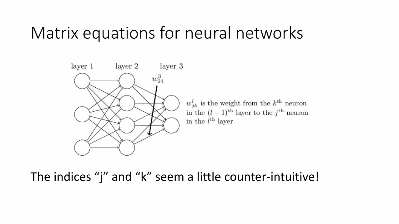
Matrix equations for neural networks

The indices “j” and “k” seem a little counter-intuitive!

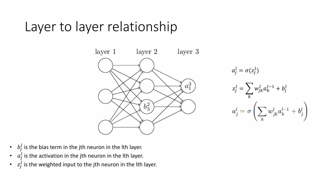
Layer to layer relationship

• 𝑏𝑗𝑙 is the bias term in the jth neuron in the lth layer.

• 𝑎𝑗𝑙 is the activation in the jth neuron in the lth layer.

• 𝑧𝑗𝑙 is the weighted input to the jth neuron in the lth layer.

𝑎𝑗𝑙 = 𝜎(𝑧𝑗

𝑙)

𝑧𝑗𝑙 =

𝑘

𝑤𝑗𝑘𝑙 𝑎𝑘

𝑙−1 + 𝑏𝑗𝑙

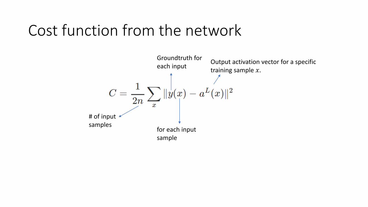
Cost function from the network

# of input samples

for each input sample

Output activation vector for a specific training sample 𝑥.

Groundtruth for each input

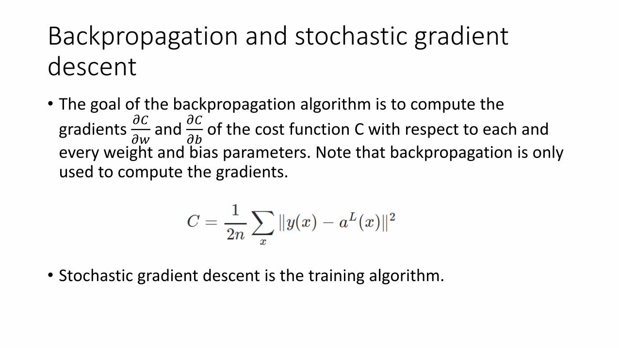
Backpropagation and stochastic gradient descent• The goal of the backpropagation algorithm is to compute the

gradients 𝜕𝐶

𝜕𝑤and

𝜕𝐶

𝜕𝑏of the cost function C with respect to each and

every weight and bias parameters. Note that backpropagation is only used to compute the gradients.

• Stochastic gradient descent is the training algorithm.

Assumptions on the cost function

1. We assume that the cost function can be written as the average over

the cost functions from individual training samples: 𝐶 =1

𝑛σ𝑥 𝐶𝑥. The

cost function for the individual training sample is given by 𝐶𝑥 =1

2𝑦 𝑥 − 𝑎𝐿 𝑥 2.

- why do we need this assumption? Backpropagation will only allow us to compute the gradients with respect to a single training

sample as given by 𝜕𝐶𝑥

𝜕𝑤and

𝜕𝐶𝑥

𝜕𝑏. We then recover

𝜕𝐶

𝜕𝑤and

𝜕𝐶

𝜕𝑏by averaging

the gradients from the different training samples.

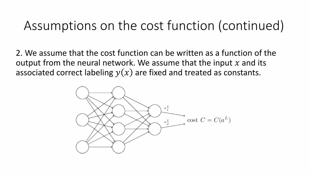
Assumptions on the cost function (continued)

2. We assume that the cost function can be written as a function of the output from the neural network. We assume that the input 𝑥 and its associated correct labeling 𝑦 𝑥 are fixed and treated as constants.

Hadamard product

• Let 𝑠 and 𝑡 are two vectors. The Hadamard product is given by:

Such elementwise multiplication is also referred to as schur product.

Backpropagation

• Our goal is to compute the partial derivatives 𝜕𝐶

𝜕𝑤𝑗𝑘𝑙 and

𝜕𝐶

𝜕𝑏𝑗𝑙 .

• We compute some intermediate quantities while doing so:

𝛿𝑗𝑙 =

𝜕𝐶

𝜕𝑧𝑗𝑙

Four equations of the BP (backpropagation)

Chain Rule in differentiation

• In order to differentiate a function z = 𝑓 𝑔 𝑥 w.r.t 𝑥, we can do the following:

Let y = 𝑔 𝑥 , 𝑧 = 𝑓 𝑦 ,𝑑𝑧

𝑑𝑥=

𝑑𝑧

𝑑𝑦×

𝑑𝑦

𝑑𝑥

Chain Rule in differentiation (vector case)

Let 𝑥 ∈ ℝ𝑚, 𝑦 ∈ ℝ𝑛, g maps from ℝ𝑚 to ℝ𝑛, and 𝑓 maps from ℝ𝑛 to ℝ. If 𝑦 = 𝑔 𝑥 and 𝑧 = 𝑓 𝑦 , then

𝜕𝑧

𝜕𝑥𝑖=

𝑘

𝜕𝑧

𝜕𝑦𝑘

𝜕𝑦𝑘𝜕𝑥𝑖

Chain Rule in differentiation (computation graph)

𝜕𝑧

𝜕𝑥=

𝑗:𝑥∈𝑃𝑎𝑟𝑒𝑛𝑡 𝑦𝑗 ,

𝑦𝑗∈𝐴𝑛𝑐𝑒𝑠𝑡𝑜𝑟 (𝑧)

𝜕𝑧

𝜕𝑦𝑗

𝜕𝑦𝑗

𝜕𝑥𝑥 𝑧

𝑦1

𝑦2

𝑦3

BP1

Here L is the last layer.

𝛿𝐿 =𝜕𝐶

𝜕𝑧𝐿, 𝜎′ 𝑧𝐿 =

𝜕 𝜎 𝑧𝐿

𝜕𝑧𝐿, 𝛻𝑎𝐶 =

𝜕𝐶

𝜕𝑎𝐿=

𝜕𝐶

𝜕𝑎1𝐿 ,

𝜕𝐶

𝜕𝑎2𝐿 , … ,

𝜕𝐶

𝜕𝑎𝑛𝐿

𝑇

Proof:

𝛿𝑗𝐿 =

𝜕𝐶

𝜕𝑧𝑗𝐿 = σ𝑘

𝜕𝐶

𝜕𝑎𝑘𝐿

𝜕𝑎𝑘𝐿

𝜕𝑧𝑗𝐿 =

𝜕𝐶

𝜕𝑎𝑗𝐿

𝜕𝑎𝑗𝐿

𝜕𝑧𝑗𝐿 when 𝑗 ≠ 𝑘, the term

𝜕𝑎𝑘𝐿

𝜕𝑧𝑗𝐿 vanishes.

𝛿𝑗𝐿 =

𝜕𝐶

𝜕𝑎𝑗𝐿 𝜎′(𝑧𝑗

𝐿)

Thus we have

𝜕𝐿 =𝜕𝐶

𝜕𝑎𝐿⊙𝜎′(𝑧𝐿 )

𝑎𝐿 = 𝜎(𝑧𝐿)

𝐶 = 𝑓(𝑎𝐿)

𝐿𝑎𝑦𝑒𝑟 𝐿 − 1𝐿𝑎𝑦𝑒𝑟 𝐿 − 1 𝐿𝑎𝑦𝑒𝑟 𝐿

BP2

𝜕𝑙 = 𝑤𝑙+1 𝑇𝛿𝑙+1 ⊙𝜎′ 𝑧𝑙

Proof:

𝛿𝑗𝑙 =

𝜕𝐶

𝜕𝑧𝑗𝑙 = σ𝑘

𝜕𝐶

𝜕𝑧𝑘𝑙+1

𝜕𝑧𝑘𝑙+1

𝜕𝑧𝑗𝑙 = σ𝑘

𝜕𝑧𝑘𝑙+1

𝜕𝑧𝑗𝑙 𝛿𝑘

𝑙+1

𝑧𝑘𝑙+1 = σ𝑗𝑤𝑘𝑗

𝑙+1𝑎𝑗𝑙 + 𝑏𝑘

𝑙 = σ𝑗𝑤𝑘𝑗𝑙+1𝜎 𝑧𝑗

𝑙 + 𝑏𝑘𝑙

By differentiating we have:𝜕𝑧𝑘

𝑙+1

𝜕𝑧𝑗𝑙 = 𝑤𝑘𝑗

𝑙+1𝜎′ 𝑧𝑗𝑙

𝛿𝑗𝑙 = σ𝑘𝑤𝑘𝑗

𝑙+1𝛿𝑘𝑙+1𝜎′ 𝑧𝑗

𝑙

𝑧𝑙+1 = 𝑤𝑙+1𝑎𝑙 + 𝑏𝑙+1

𝐿𝑎𝑦𝑒𝑟 𝑙 𝐿𝑎𝑦𝑒𝑟 𝑙 + 1

BP3

𝜕𝐶

𝜕𝑏𝑗𝑙 = 𝛿𝑗

𝑙

Proof:𝜕𝐶

𝜕𝑏𝑗𝑙 =

𝑘

𝜕𝐶

𝜕𝑧𝑘𝑙

𝜕𝑧𝑘𝑙

𝜕𝑏𝑗𝑙 =

𝜕𝐶

𝜕𝑧𝑗𝑙

𝜕𝑧𝑗𝑙

𝜕𝑏𝑗𝑙

= 𝛿𝑗𝑙𝜕 σ𝑘 𝑤𝑗𝑘𝑎𝑘

𝑙−1 + 𝑏𝑗𝑙

𝜕𝑏𝑗= 𝛿𝑗

𝑙

𝑧𝑙 = 𝑤𝑙𝑎𝑙−1 + 𝑏𝑙

𝐿𝑎𝑦𝑒𝑟 𝑙-1 𝐿𝑎𝑦𝑒𝑟 𝑙

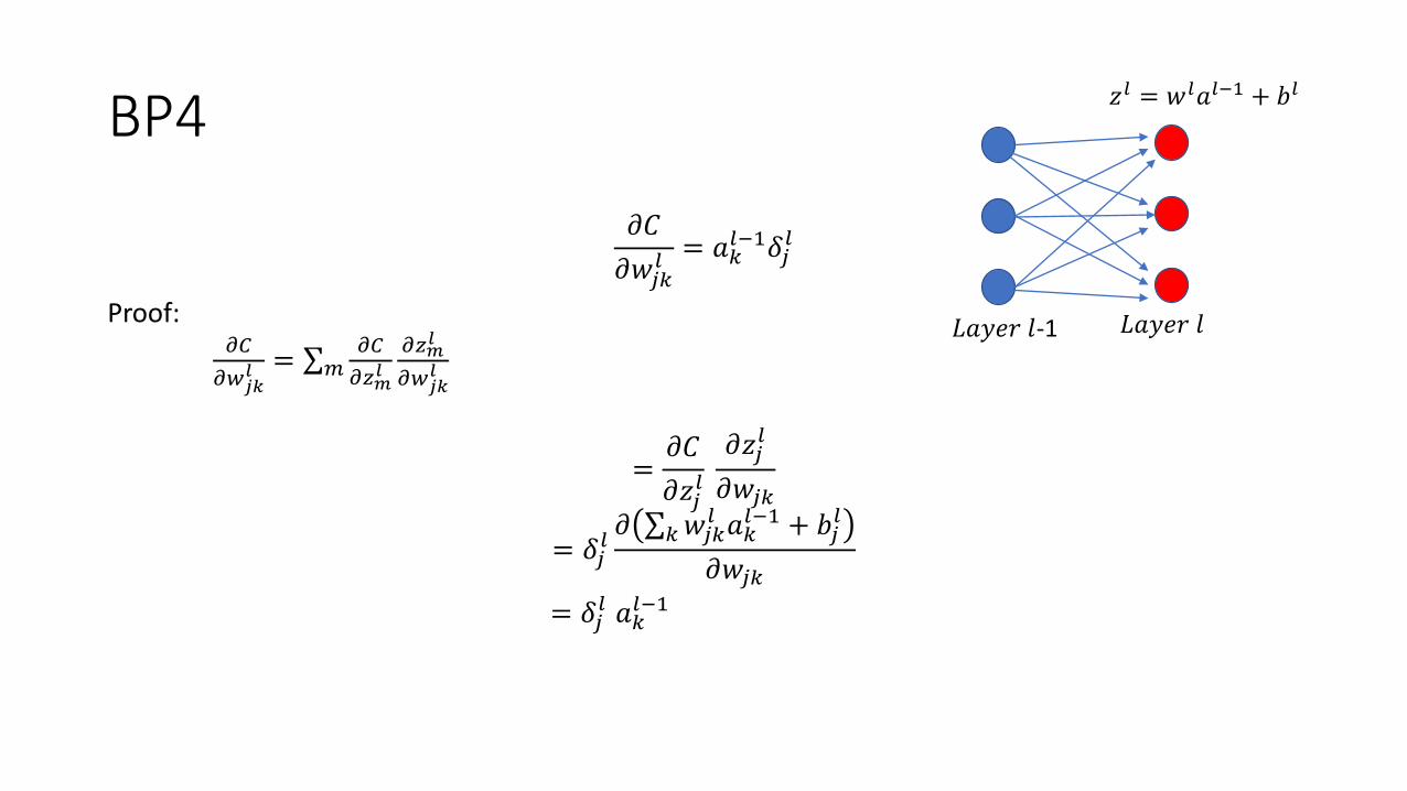
BP4

𝜕𝐶

𝜕𝑤𝑗𝑘𝑙 = 𝑎𝑘

𝑙−1𝛿𝑗𝑙

Proof: 𝜕𝐶

𝜕𝑤𝑗𝑘𝑙 = σ𝑚

𝜕𝐶

𝜕𝑧𝑚𝑙

𝜕𝑧𝑚𝑙

𝜕𝑤𝑗𝑘𝑙

=𝜕𝐶

𝜕𝑧𝑗𝑙

𝜕𝑧𝑗𝑙

𝜕𝑤𝑗𝑘

= 𝛿𝑗𝑙𝜕 σ𝑘𝑤𝑗𝑘

𝑙 𝑎𝑘𝑙−1 + 𝑏𝑗

𝑙

𝜕𝑤𝑗𝑘

= 𝛿𝑗𝑙 𝑎𝑘

𝑙−1

𝑧𝑙 = 𝑤𝑙𝑎𝑙−1 + 𝑏𝑙

𝐿𝑎𝑦𝑒𝑟 𝑙-1 𝐿𝑎𝑦𝑒𝑟 𝑙

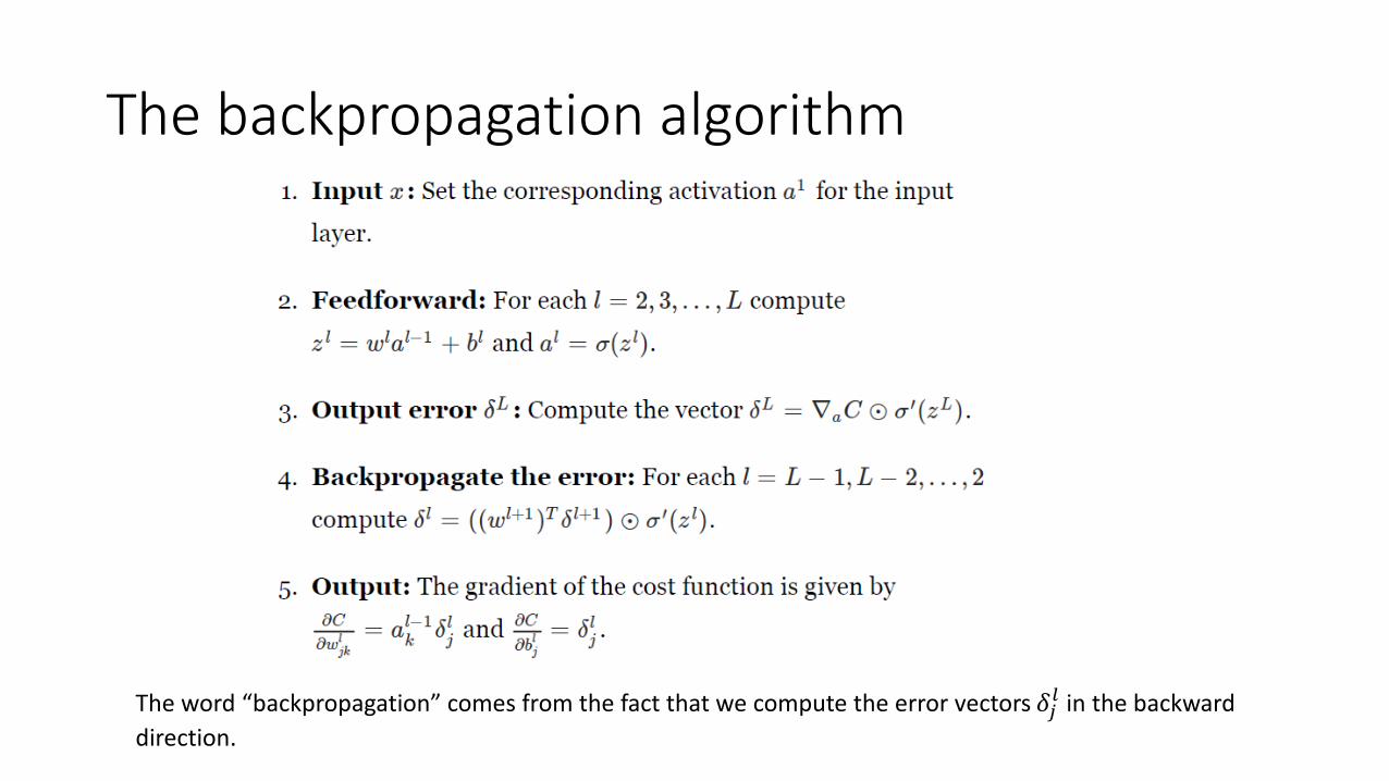
The backpropagation algorithm

The word “backpropagation” comes from the fact that we compute the error vectors 𝛿𝑗𝑙 in the backward

direction.

Stochastic gradient descent with BP

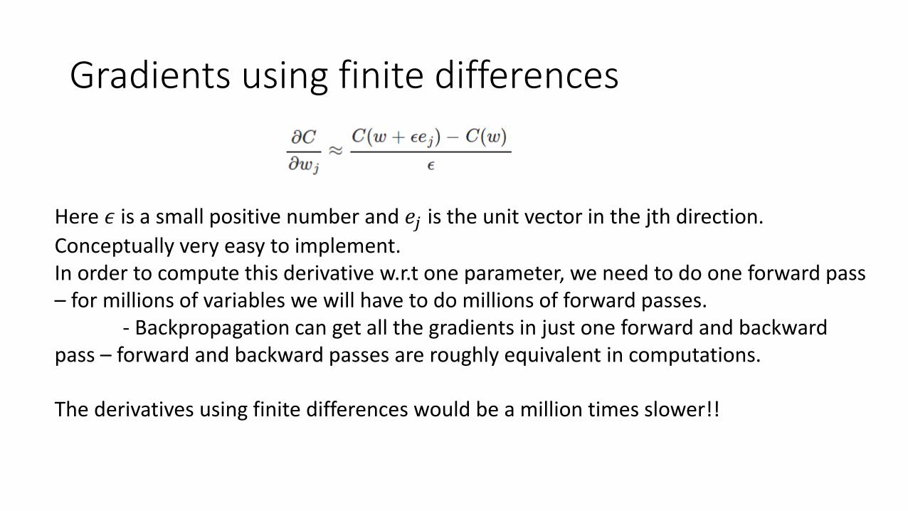
Gradients using finite differences

Here 𝜖 is a small positive number and 𝑒𝑗 is the unit vector in the jth direction.

Conceptually very easy to implement.In order to compute this derivative w.r.t one parameter, we need to do one forward pass – for millions of variables we will have to do millions of forward passes.

- Backpropagation can get all the gradients in just one forward and backward pass – forward and backward passes are roughly equivalent in computations.

The derivatives using finite differences would be a million times slower!!

Backpropagation – the big picture

• To compute the total change in C we need to consider all possible paths from the weight to the cost.

• We are computing the rate of change of C w.r.t a weight w.

• Every edge between two neurons in the network is associated with a rate factor that is just the ratio of partial derivatives of one neurons activation with respect to another neurons activation.

• The rate factor for a path is just the product of the rate factors of the edges in the path.

• The total change is the sum of the rate factors of all the paths from the weight to the cost.

Thank You

Chain Rule in differentiation (vector case)

Let 𝑥 ∈ ℝ𝑚, 𝑦 ∈ ℝ𝑛, g maps from ℝ𝑚 to ℝ𝑛, and 𝑓 maps from ℝ𝑛 to ℝ. If 𝑦 = 𝑔 𝑥 and 𝑧 = 𝑓 𝑦 , then

𝜕𝑧

𝜕𝑥𝑖=

𝑘

𝜕𝑧

𝜕𝑦𝑘

𝜕𝑦𝑘𝜕𝑥𝑖

𝛻𝑥𝑧 =𝜕𝑦

𝜕𝑥

𝑇𝛻𝑦𝑧

Here 𝜕𝑦

𝜕𝑥is the 𝑛 ×𝑚 Jacobian matrix of 𝑔.

Source: http://math.arizona.edu/~calc/Rules.pdf

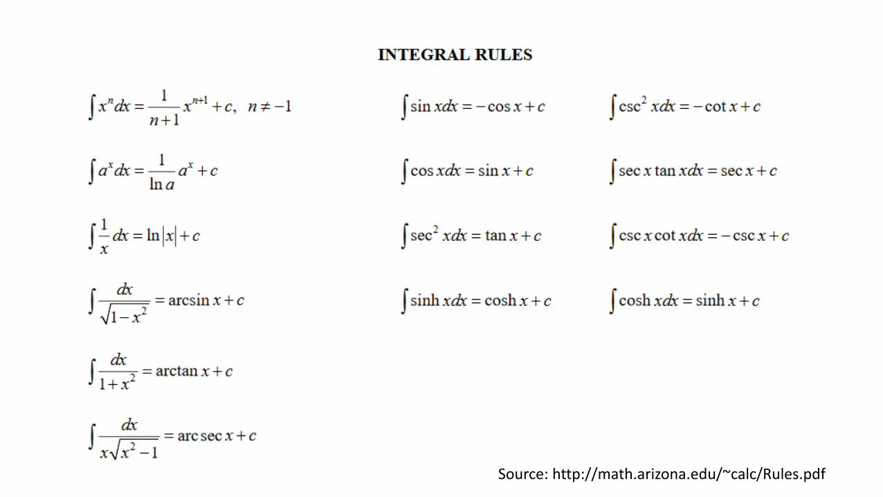
Source: http://math.arizona.edu/~calc/Rules.pdf