The Backpropagation Algorithm - Harvard Universityasaxe/papers/backpropagation.pdf–...

The Backpropagation Algorithm

Psych 209

Andrew Saxe

Backpropagation from 30,000ft

•  Learning algorithm for arbitrary, deep, complicated neural networks

•  You’ve used it! – Google/Microsoft/Yahoo voice recognition,

image search, machine translation, …

•  The core idea behind many psychology & neuroscience models

Backpropagation from 30,000ft

•  Can be written down in one line of math:

•  Sort of like Newton’s laws – Three simple equations

– But endless implications and consequences

•  Need to understand it intuitively at many levels

ΔW = −λ∂E∂W

Two meanings

•  “Backprop” technically refers to a specific algorithm

•  But often used as shorthand for a much broader framework with a galaxy of associated ideas and commitments

•  Important not to confuse backprop-the-algorithm with backprop-the-framework—this has caused trouble in the past

•  Your job is to learn backprop-the-framework

Levels of analysis

•  Computational level – Learning as optimization

– Gradient descent

•  Algorithmic level – Backprop-the-algorithm

•  Implementation level

Psych/neuro conceptual implications

•  Backprop-as-framework comes with a host of ideas about the brain and mind:

•  E.g., learning and development are –  Incremental –  Experience-driven –  Encoded in synaptic weights

•  Computation is –  Parallel –  Distributed

Today

•  Build up to learning in arbitrary deep network

1.  One parallel layer

2.  Many serial layers

3.  Nonlinearities

4.  Pandemonium! The general case

The pattern associator

i ∈ RN1t ∈ RN2

W

Input Output Target

o∈ RN2

One layer learning

i ∈ RN1t ∈ RN2

Input Output Target

o∈ RN2

.2

.5

-1

0

1

1

.2

-.1

-2

.1

Forward propagation Input Output Target

.2

.5

-1

0

1

.5

1

.2

-.1

-2

.1 o = wjij∑

Target Feedback

i ∈ RN1t ∈ RN2

Input Output Target

o∈ RN2

.2

.5

-1

0

1

.5 1

1

.2

-.1

-2

.1

Error signal

i ∈ RN1t ∈ RN2

Input Output Target

o∈ RN2

.2

.5

-1

0

1

.5 1

1

.2

-.1

-2

.1 Error = .5

How to fix?

i ∈ RN1t ∈ RN2

Input Output Target

o∈ RN2

.2

.5

-1

0

1

.5 1

1

.2

-.1

-2

.1 Error = .5

Lots of choices

•  How can we choose?

•  Maybe: make small change that most rapidly decreases the error

Lots of choices

•  How can we choose?

•  Maybe: make small change that most rapidly decreases the error

•  This is called Gradient Descent

Gradient Descent Learning

•  Make small change in weights that most rapidly improves task performance

•  Change each weight in proportion to the gradient of the error ΔW = −λ

∂E∂W

Optimization view of learning

•  The network and training data together define an error function, say, squared error

E(t,w,i) = (t-o)2

•  Learning is just minimizing this function w.r.t. w

w* = argminw E(t,w,i)

Gradient Descent

http://blog.datumbox.com/wp-content/uploads/2013/10/gradient-descent.png

w1 w2

Err

or

ΔW = −λ∂E∂W

Delta rule derivation

E = (t −o)2

= (t − wj∑ ij )2

= (t −wi)2


E = (t −o)2

= (t − wj∑ ij )2

= (t −wi)2

∂E∂wk

= −2(t −o) ∂E∂wk

o

= −2(t −o) ∂E∂wk

wj∑ ij

= −2(t −o)ik


E = (t −o)2

= (t − wj∑ ij )2

= (t −wi)2

∂E∂wk

= −2(t −o) ∂E∂wk

o

= −2(t −o) ∂E∂wk

wj∑ ij

= −2(t −o)ik

Δw = λ(t −o)iT = λeiTDelta rule:

What about deep networks?

•  Delta rule only makes sense for one layer!

•  How can we learn in deep, multilayer networks?

What about deep networks?

•  Delta rule only makes sense for one layer!

•  How can we learn in deep, multilayer networks?

•  Why would we want deep, multilayer networks?

Why deep networks?

•  Shallow networks can’t represent any function, eg, XOR

•  Anatomically and physiologically, the brain is deep

•  Empirically, deep networks just work better

Two fundamental topologies

Parallel Serial


Parallel Serial

Delta rule ???

Gradient descent learning rule:

Many layer learning

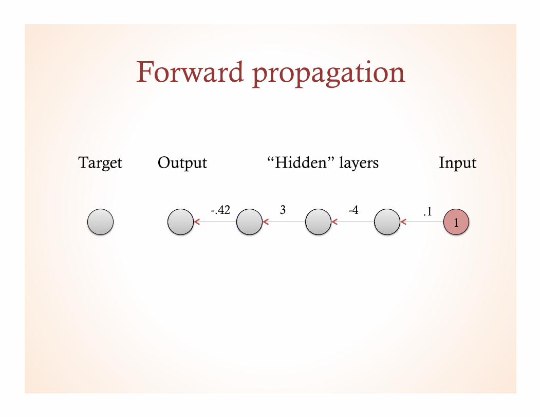
Input Output Target “Hidden” layers

Forward propagation

.1 1


.1 -4 3 -.42 -.4 -1.2 .5

o = w4w3w2w1i = wk∏( )i

Target feedback

.1 1 1


.1 -4 3 -.42 -.4 -1.2 .5

Error signal

.1 1 1


.1 -4 3 -.42 -.4 -1.2 .5

Error = .5

How to fix?

.1 1 1


.1 -4 3 -.42 -.4 -1.2 .5

Error = .5

How to fix?

.1 1 1


.6 -4 3 -.42 -.4 -1.2 .5

Error = .5

How to fix?

.1 1 1


.6 -4 3 -.42 -2.4 -7.2 3

Error = -2

How to fix?

.1 1 1


.1 -4 3 -.42 -.4 -1.2 .5

Error = .5 Increase?

How to fix?

.1 1 1


.1 -2 3 -.42 -.4 -1.2 .5

Error = .5

How to fix?

.1 1 1


.1 -2 3 -.42 -.2 -.6 .25

Error = .75

How to fix?

.1 1 1


.1 -2 3 -.42 -.2 -.6 .25

Must consider effect of all upstream weights to know how to change any given weight! In a deep network, weights are coupled


Parallel Serial

Sum of variables Weights are independent

Product of variables Weights are coupled

o = wk∏( )io = wjij∑

The solution: Backpropagation

•  Send a signal from the output of the network back down towards the input

•  This signal will encode how changing a weight will propagate to the output

•  Then use delta-like rule as usual

The solution: Backpropagation

.1 1


.1 -4 3 -.42 -.4 -1.2 .5

Input

Forward propagation Back propagation

Error Delta Hidden Activity

Δwj = λδ j+1hj

Forward propagation

.1 1


.1 -4 3 -.42 -.4 -1.2 .5

Target feedback

.1 1 1


.1 -4 3 -.42 -.4 -1.2 .5

Error signal

.1 1 1


.1 -4 3 -.42 -.4 -1.2 .5

Error = .5

Backpropagation

.1 1

Input Output “Hidden” layers

.1 -4 3 -.42 -.4 -1.2 .5

.1 -4 3 -.42 -.63 -.21 .5 2.5

1

Target

Error à

δ j = wj+1δ j+1

Backpropagation

.1 1

Input Output “Hidden” layers

.1 -4 3 -.42 -.4 -1.2 .5

.1 -4 3 -.42 -.63 -.21 .5 2.5

Activations

Deltas

Δwj = λδ j+1hjLearning rule:

Derivation as gradient descent

∂∂w2

(t −o)2 = −2(t −o) ∂∂w2

w4w3w2w1i

= −2(t −o)w4w3w1i

δ3 h2

Δwj = λδ j+1hjLearning rule:

Delta vs Backprop

Delta rule:

•  Requires actual error and input

•  Restricted to one layer

Backprop:

(where j indexes the layer)

•  Uses backpropagated error and hidden layer activity

•  Works in deep network

Δwj = λδ j+1hjΔw = λe iT

•  Both implement gradient descent

Nonlinearities

•  So far have just looked at linear networks

•  Linear networks cannot represent complicated functions (like XOR)

•  Introduce neural nonlinearity or “activation function”

Activation function

w

∑

f(…)

Net Input

Activation

o = f wjij∑( )

Gradient learning with nonlinearities

∂E∂wk

= −2(t −o) ∂E∂wk

f wjij∑( )

= −2(t −o) $f (n) ∂E∂wk

wjij∑

= −2(t −o) $f (n)ik

Δw = λe !f (n)iTScaled delta rule:

Beyond the chain…

x ∈ RN1y ∈ RND+1

. . .

h2 ∈ RN3x

W 1W 2WD

f (W 1x)f (WDhD )

f (x)

f (W 2h1)f (WD−1hD−1)

Andrew Saxe 55

Now for the general case: a mixture of serial and parallel structure with nonlinearities

Matrix notation

x ∈ RN1y ∈ RND+1

. . .

h2 ∈ RN3x

W 1W 2WD

f (W 1x)f (WDhD )

f (x)

f (W 2h1)f (WD−1hD−1)

Andrew Saxe 56

Matrix notation

o = f (WD f (WD−1... f (W 2 f (W 1i))...))

Andrew Saxe 57

Column vector Column vector

Nonlinearity applied elementwise

Matrix multiplication

Putting the pieces together

•  Single layer parallel: the delta rule

•  Multilayer serial: backpropagation

•  Nonlinearities: scale by derivative

Putting the pieces together

. . .

Forward prop input to compute hidden activities, net inputs, output

Back prop error to compute deltas

ΔW j = λδ j+1hTjLearning rule:

Backpropagation

. . .

ΔW j = λδ j+1hTjLearning rule:

δ j = W j( )Tδ j+1

!"#

$%&•

'f (nj )

δD = −(t −o)• "f (nD )

Summary

•  Computational level –  Optimization view of learning –  Gradient descent

•  Algorithmic level –  Backprop-as-algorithm

•  Implementation level –  Haven’t touched on it –  Few do! –  Not at all obvious how to implement in the brain

The Backpropagation Algorithm - Harvard Universityasaxe/papers/backpropagation.pdf–...

Documents

Transcript of The Backpropagation Algorithm - Harvard Universityasaxe/papers/backpropagation.pdf–...