Patrick Laug & Houman Borouchaki Gamma3 project -team ( Inria and UTT)

Houman OwhadiThe worst case approach to UQ
“The gods to-day stand friendly, that we may,Lovers of peace, lead on our days to age!But, since the affairs of men rests still uncertain,Let’s reason with the worst that may befall.”
Julius Caesar, Act 5, Scene 1William Shakespeare (1564 –1616)

You want to certify that
Problem
and

You want to certify that
Problem
and
You only know

Worst and best caseoptimal bounds P[G(X) ≥ a]given available information.
Compute

I. Elishakoff and M. Ohsaki. Optimization and Anti-Optimization of Structures Under Uncertainty. World Scientific, London, 2010.
Saltelli, A.; Ratto, M.; Andres, T.; Campolongo, F.; Cariboni, J.; Gatelli, D.; Saisana, M.; Tarantola, S. (2008). Global Sensitivity Analysis: The Primer. John Wiley & Sons.
Global Sensitivity Analysis
A. Ben-Tal, L. El Ghaoui, and A.Nemirovski. Robust optimization. PrincetonSeries in Applied Mathematics. Princeton University Press, Princeton, NJ, 2009
D. Bertsimas, D. B. Brown, and C. Caramanis. Theory and applications of robustoptimization. SIAM Rev., 53(3):464–501, 2011
Robust Optimization
A. Ben-Tal and A. Nemirovski. Robust convex optimization. Math. Oper. Res.,23(4):769–805, 1998
Optimal Uncertainty QuantificationH. Owhadi, C. Scovel, T. J. Sullivan, M. McKerns, and M. Ortiz. Optimal Uncertainty Quantification. SIAM Review, 55(2):271–345, 2013.

Set based design in the aerospace industry
Bernstein JI (1998) Design methods in the aerospace industry: looking for evidence of set-based practices. Master’s thesis. Massachusetts Institute of Technology, Cambridge, MA.
Set based design/analysis
B. Rustem and Howe M. Algorithms for Worst-Case Design and Applications toRisk Management. Princeton University Press, Princeton, 2002.
David J. Singer, PhD., Captain Norbert Doerry, PhD., and Michael E. Buckley,” What is Set-Based Design? ,” Presented at ASNE DAY 2009, National Harbor, MD., April 8-9, 2009. Also published in ASNE Naval Engineers Journal, 2009 Vol 121 No 4, pp. 31-43.


P. L. Chebyshev1821-1894
M. G. Krein1907-1989
A. A. Markov1856-1922

Answer

Answer
Markov’s inequality

History of classical inequalitiesS. Karlin and W. J. Studden. Tchebycheff Systems: With Applications in Analysisand Statistics. Pure and Applied Mathematics, Vol. XV. Interscience PublishersJohn Wiley & Sons, New York-London-Sydney, 1966.
Theory of majorization
A. W. Marshall and I. Olkin. Inequalities: Theory of Majorization and its Appli-cations, volume 143 of Mathematics in Science and Engineering. Academic PressInc. [Harcourt Brace Jovanovich Publishers], New York, 1979
M. G. Krein. The ideas of P. L. Cebysev and A. A. Markov in the theory of limitingvalues of integrals and their further development. In E. B. Dynkin, editor, Elevenpapers on Analysis, Probability, and Topology, American Mathematical SocietyTranslations, Series 2, Volume 12, pages 1–122. American Mathematical Society,New York, 1959.
Classical Markov-Krein theorem and classical works of Krein, Markov and Chebyshev

Connections between Chebyshev inequalities and optimization theoryH. J. Godwin. On generalizations of Tchebychef’s inequality. J. Amer. Statist.Assoc., 50(271):923–945, 1955.
K. Isii. On a method for generalizations of Tchebycheff’s inequality. Ann. Inst.Statist. Math. Tokyo, 10(2):65–88, 1959.
K. Isii. On sharpness of Tchebycheff-type inequalities. Ann. Inst. Statist. Math.,14(1):185–197, 1962/1963.
A. W. Marshall and I. Olkin. Multivariate Chebyshev inequalities. Ann. Math.Statist., 31(4):1001–1014, 1960.
A. W. Marshall and I. Olkin. Inequalities: Theory of Majorization and its Appli-cations, volume 143 of Mathematics in Science and Engineering. Academic PressInc. [Harcourt Brace Jovanovich Publishers], New York, 1979
I. Olkin and J. W. Pratt. A multivariate Tchebycheff inequality. Ann. Math.Statist, 29(1):226–234, 1958.
K. Isii. The extrema of probability determined by generalized moments. I. Boundedrandom variables. Ann. Inst. Statist. Math., 12(2):119–134; errata, 280, 1960.
L. Vandenberghe, S. Boyd, and K. Comanor. Generalized Chebyshev bounds viasemidefinite programming. SIAM Rev., 49(1):52–64 (electronic), 2007
Connection between Chebyshev inequalities and optimization theory
H. Joe. Majorization, randomness and dependence for multivariate distributions.Ann. Probab., 15(3):1217–1225, 1987.
J. E. Smith. Generalized Chebychev inequalities: theory and applications in decisionanalysis. Oper. Res., 43(5):807–825, 1995.
D. Bertsimas and I. Popescu. Optimal inequalities in probability theory: a convexoptimization approach. SIAM J. Optim., 15(3):780–804 (electronic), 2005.
E. B. Dynkin. Sufficient statistics and extreme points. Ann. Prob., 6(5):705–730,1978.
A. F. Karr. Extreme points of certain sets of probability measures, with applications.Math. Oper. Res., 8(1):74–85, 1983.

Stochastic linear programming and Stochastic Optimization
P. Kall. Stochastric programming with recourse: upper bounds and moment problems:a review. Mathematical research, 45:86–103, 1988
A. Madansky. Bounds on the expectation of a convex function of a multivariaterandom variable. The Annals of Mathematical Statistics, pages 743–746, 1959
A. Madansky. Inequalities for stochastic linear programming problems. Manage-ment science, 6(2):197–204, 1960.
G. B. Dantzig. Linear programming under uncertainty. Management Sci., 1:197–206, 1955.
J. R. Birge and R. J.-B. Wets. Designing approximation schemes for stochasticoptimization problems, in particular for stochastic programs with recourse. Math.Prog. Stud., 27:54–102, 1986
Y. Ermoliev, A. Gaivoronski, and C. Nedeva. Stochastic optimization problemswith incomplete information on distribution functions. SIAM Journal on Controland Optimization, 23(5):697–716, 1985
C. C. Huang, W. T. Ziemba, and A. Ben-Tal. Bounds on the expectation of a convexfunction of a random variable: With applications to stochastic programming.Operations Research, 25(2):315–325, 1977.
J. Zjackovja. On minimax solutions of stochastic linear programming problems.Casopis Pest. Mat., 91:423–430, 1966.

Chance constrained/distributionally robust optimization
J. Goh and M. Sim. Distributionally robust optimization and its tractable approximations. Oper. Res., 58(4, part 1):902–917, 2010
R. I. Bot N. Lorenz, and G. Wanka. Duality for linear chance-constrained optimizationproblems. J. Korean Math. Soc., 47(1):17–28, 2010.
W. Wiesemann, D. Kuhn, and M. Sim. Distributionally robust convex optimization.Oper. Res., 62(6):1358–1376, 2014.
L. Xu, B. Yu, and W. Liu. The distributionally robust optimization reformulationfor stochastic complementarity problems. Abstr. Appl. Anal., pages 7, 2014.
S. Zymler, D. Kuhn, and B. Rustem. Distributionally robust joint chance constraintswith second-order moment information. Math. Program., 137(1-2, Ser.A):167–198, 2013.
A. A. Gaivoronski. A numerical method for solving stochastic programming problemswith moment constraints on a distribution function. Annals of OperationsResearch, 31(1):347–369, 1991.
G. A. Hanasusanto, V. Roitch, D. Kuhn, and W. Wiesemann. A distributionallyrobust perspective on uncertainty quantification and chance constrained programming.Mathematical Programming, 151(1):35–62, 2015
Value at Risk
Artzner, P.; Delbaen, F.; Eber, J. M.; Heath, D. (1999). Coherent Measures of Risk. Mathematical Finance 9 (3): 203.
W. Chen, M. Sim, J. Sun, and C.-P. Teo. From CVaR to uncertainty set: implicationsin joint chance-constrained optimization. Oper. Res., 58(2):470–485, 2010.

Optimal Uncertainty Quantification
S. Han, M. Tao, U. Topcu, H. Owhadi, and R. M. Murray. Convex optimal uncertaintyquantification. SIAM Journal on Optimization, 25(23):1368–1387, 2015.
S. Han, U. Topcu, M. Tao, H. Owhadi, and R. Murray. Convex optimal uncertaintyquantification: Algorithms and a case study in energy storage placement for powergrids. In American Control Conference (ACC), 2013, pages 1130–1137. IEEE,2013
H. Owhadi, C. Scovel, T. J. Sullivan, M. McKerns, and M. Ortiz. Optimal Uncertainty Quantification. SIAM Review, 55(2):271–345, 2013.
T. J. Sullivan, M. McKerns, D. Meyer, F. Theil, H. Owhadi, and M. Ortiz. Optimaluncertainty quantification for legacy data observations of Lipschitz functions.ESAIM Math. Model. Numer. Anal., 47(6):1657–1689, 2013.
J Chen, MD Flood, R Sowers. Measuring the Unmeasurable: An Application of Uncertainty Quantification to Financial Portfolios, OFR WP, 2015
L Ming, W Chenglin. An improved algorithm for convex optimal uncertainty quantification with polytopic canonical form. Control Conference (CCC), 2015
H. Owhadi and Clint Scovel. Extreme points of a ball about a measure with finite support (2015). arXiv:1504.06745
H. Owhadi, C. Scovel and T. Sullivan. Brittleness of Bayesian Inference under Finite Information in a Continuous World. Electronic Journal of Statistics, vol 9, pp 1-79, 2015. arXiv:1304.6772

Our proof relies on• Winkler (1988, Extreme points of moment sets)• Follows from an extension of Choquet theory (Phelps 2001, lectures on Choquet’s
theorem) by Von Weizsacker & Winkler (1979, Integral representation in the set ofsolutions of a generalized moment problem)
• Kendall (1962, Simplexes & Vector lattices)
G. Winkler. On the integral representation in convex noncompact sets of tightmeasures. Mathematische Zeitschrift, 158(1):71–77, 1978
G. Winkler. Extreme points of moment sets. Math. Oper. Res., 13(4):581–587,1988.
H. von Weizsacker and G. Winkler. Integral representation in the set of solutionsof a generalized moment problem. Math. Ann., 246(1):23–32, 1979/80.
D. G. Kendall. Simplexes and vector lattices. J. London Math. Soc., 37(1):365–371,1962.

Theorem
H. Owhadi, C. Scovel, T. J. Sullivan, M. McKerns, and M. Ortiz. Optimal Uncertainty Quantification. SIAM Review, 55(2):271–345, 2013.

Further Reduction of optimization variables

McDiarmid inequality’s
Another example: Optimal concentration inequality H. Owhadi, C. Scovel, T. J. Sullivan, M. McKerns, and M. Ortiz. Optimal Uncertainty Quantification. SIAM Review, 55(2):271–345, 2013.

Reduction of optimization variables
Theorem

Theorem m = 2
C = (1, 1)hC(s) = a− (1− s1)D1 − (1− s2)D2
Explicit Solution m=2

Theorem m = 2
Corollary
Explicit Solution m=2

μ
f
A
Each piece of information is a constrainton an optimization problem.
Optimization concepts (binding, active) transfer to UQ concepts
Non bindingconstraint
Binding but nonactive constraint
Active constraint
Extremizer/Worst case scenario

Optimal Hoeffding= Optimal McDiarmid for m=2

Theorem m = 3Explicit Solution m=3

F min( Yield Strain - Axial Strain )
Ground Acceleration
We want to certify that
Seismic Safety Assessment of a Truss Structure

Power Spectrum
0
0.2
0.4
0.6
0.8
1
1.2
1.4
1.6
0.1 0.6 1.1 1.6 2.1 2.6 3.1 3.6 4.1 4.6 5.1 5.6 6.1 6.6 7.1 7.6 8.1 8.6 9.1 9.6
Frequency
Am
plitu
de
Mean PSObserved PS

Power Spectrum
0
0.2
0.4
0.6
0.8
1
1.2
1.4
0.1 0.6 1.1 1.6 2.1 2.6 3.1 3.6 4.1 4.6 5.1 5.6 6.1 6.6 7.1 7.6 8.1 8.6 9.1 9.6
Frequency
Am
plitu
de
Mean PSObserved PS

Power Spectrum
0
0.2
0.4
0.6
0.8
1
1.2
1.4
0.1 0.6 1.1 1.6 2.1 2.6 3.1 3.6 4.1 4.6 5.1 5.6 6.1 6.6 7.1 7.6 8.1 8.6 9.1 9.6
Frequency
Am
plitu
de
Mean PSObserved PS

Filtered White Noise Model
White noise
Ground acceleration
Filter0
0.2
0.4
0.6
0.8
1
1.2
1.4
0.1 0.6 1.1 1.6 2.1 2.6 3.1 3.6 4.1 4.6 5.1 5.6 6.1 6.6 7.1 7.6 8.1 8.6 9.1 9.6
Frequency
Am
plitu
de
Mean PSObserved PS
N. Lama, J. Wilsona, and G. Hutchinsona. Generation of synthetic earthquake accelogramsusing seismological modeling: a review. Journal of Earthquake Engineering, 4(3):321–354, 2000.

Vulnerability Curves (vs earthquake magnitude)

Identification of the weakest elements
H. Owhadi, C. Scovel, T. J. Sullivan, M. McKerns, and M. Ortiz. Optimal Uncertainty Quantification. SIAM Review, 55(2):271–345, 2013.

Caltech Small Particle Hypervelocity Impact Range
G
Projectile velocity
Plate thickness
Plate Obliquity
Perforation area
We want to certify that
Problem

What do we know?
Projectile velocity
Plate thickness
Plate Obliquity
Thickness, obliquity, velocity: independent random variables
Mean perforation area: in between 5.5 and 7.5 mm^2
Bounds on the sensitivity of the response function w.r. to each variable

We only know
Worst case bound
Reduction calculus

What if we know the response function?
Deterministic surrogate model for the perforation area (in mm^2)

Optimal bound on the probability of non perforation
The measure of probability can be reduced to the tensorization of2 Dirac masses on thickness, obliquity and velocity
Application of the reduction calculus

The optimization variables can be reduced to the tensorizationof 2 Dirac masses on thickness, obliquity and velocity
Support Points at iteration 0

Numerical optimization
Support Points at iteration 150

Numerical optimization
Support Points at iteration 200

Velocity and obliquity marginals each collapse to a single Dirac mass. The plate thickness marginal collapses to have support on the extremes of its range.
Iteration1000
Probability non-perforation maximized by distribution supported on minimal, not maximal, impact obliquity. Dirac on velocity at a non extreme value.
Important observations
Extremizers are singular
They identify key playersi.e. vulnerabilities of the physical system
Extremizers are attractors

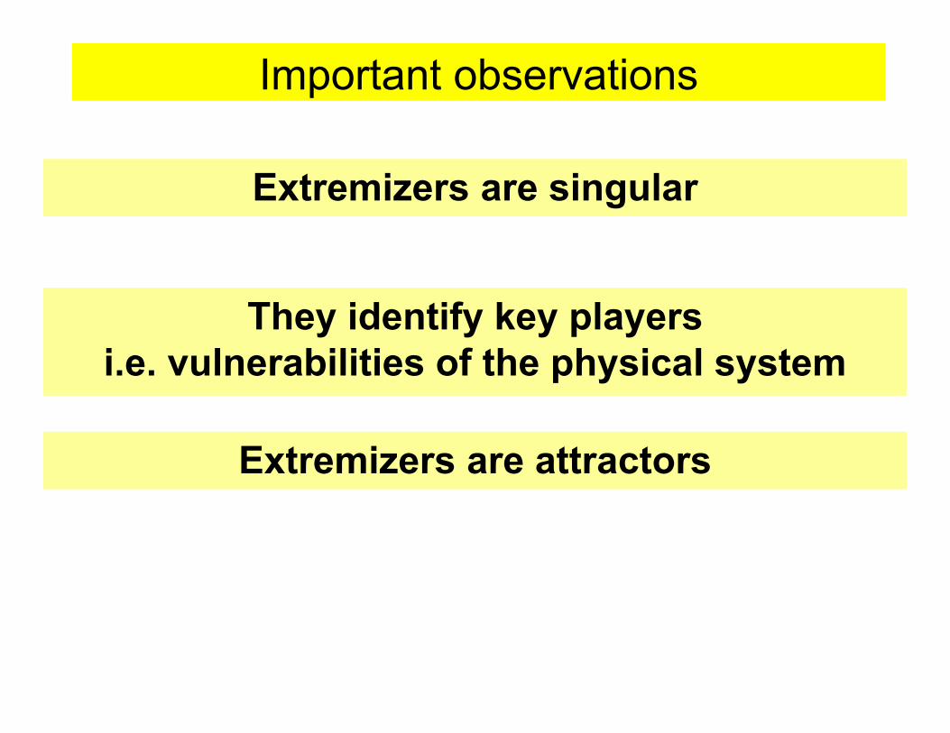
Initialization with 3 support points per marginal
Support Points at iteration 0
Initialization with 3 support points per marginal
Support Points at iteration 500

Initialization with 3 support points per marginal
Support Points at iteration 1000

Initialization with 3 support points per marginal
Support Points at iteration 2155
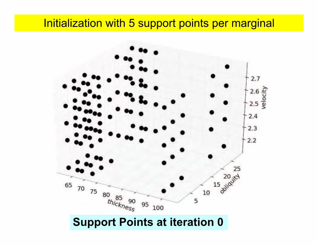
Initialization with 5 support points per marginal
Support Points at iteration 0

Initialization with 5 support points per marginal
Support Points at iteration 1000

Initialization with 5 support points per marginal
Support Points at iteration 3000

Initialization with 5 support points per marginal
Support Points at iteration 7100

Unknown response function G + Legacy data
Constraint on the mean perf. area
Modified Lipschitz continuity constraints on response function
Objective
Constraints on input variables

Legacy Data
32 data points(steel-on-aluminium shots A48–A81) from summer 2010 at Caltech’s SPHIR facility:
These constrain the value of G at 32 points
T. J. Sullivan, M. McKerns, D. Meyer, F. Theil, H. Owhadi, and M. Ortiz. Optimal uncertainty quantification for legacy data observations of Lipschitz functions. ESAIM Math. Model. Numer. Anal., 47(6):1657–1689, 2013.

The numerical results demonstrate agreement with the Markov bound
Only 2 data points out of 32 carry information about the optimal bound

Legacy Data
32 data points(steel-on-aluminium shots A48–A81) from summer 2010 at Caltech’s SPHIR facility:
Only A54 and A67 carry information
The other 30 data points carry noinformation about least upper boundand could have be ignored.
T. J. Sullivan, M. McKerns, D. Meyer, F. Theil, H. Owhadi, and M. Ortiz. Optimal uncertainty quantification for legacy data observations of Lipschitz functions. ESAIM Math. Model. Numer. Anal., 47(6):1657–1689, 2013.

What if we have model uncertainty?
What do we want?
What do we know?

PSAAP numerical model
F
Plate thickness Perforation areaProjectile velocity
Plate Obliquity=0
v
F
4.5 km/s 7 km/s0mm2
30mm2

59 data/experimental points
G
Plate thickness Perforation areaProjectile velocity
Plate Obliquity=0
v
F
4.5 km/s 7 km/s0mm2
30mm2

Confidence sausage around the model
(h, v)
PerforationArea
F
Cy

Admissible set
What we compute
Confidence sausage


v
F
4.5 km/s 7 km/s0mm2
30mm2

The extremizers led to the identification of a bug in an old model

Caltech PSAAP Center UQ analysis
P.-H. T. Kamga, B. Li, M. McKerns, L. H. Nguyen, M. Ortiz, H. Owhadi, andT. J. Sullivan. Optimal uncertainty quantification with model uncertainty andlegacy data. Journal of the Mechanics and Physics of Solids, 72:1–19, 2014
A. A. Kidane, A. Lashgari, B. Li, M. McKerns, M. Ortiz, H. Owhadi, G. Ravichan-dran, M. Stalzer, and T. J. Sullivan. Rigorous model-based uncertainty quantificationwith application to terminal ballistics. Part I: Systems with controllable inputs andsmall scatter. Journal of the Mechanics and Physics of Solids, 60(5):983–1001,2012.
M. M. McKerns, L. Strand, T. J. Sullivan, A. Fang, and M. A. G. Aivazis. Buildinga framework for predictive science. In Proceedings of the 10th Python in ScienceConference (SciPy 2011), 2011.
L. J. Lucas, H. Owhadi, and M. Ortiz. Rigorous verification, validation, uncertaintyquantification and certification through concentration-of-measure inequalities.Comput. Methods Appl. Mech. Engrg., 197(51-52):4591–4609, 2008.
H. Owhadi, C. Scovel, T. J. Sullivan, M. McKerns, and M. Ortiz. Optimal Uncertainty Quantification. SIAM Review, 55(2):271–345, 2013.
T. J. Sullivan, M. McKerns, D. Meyer, F. Theil, H. Owhadi, and M. Ortiz. Optimal uncertainty quantification for legacy data observations of Lipschitz functions. ESAIM Math. Model. Numer. Anal., 47(6):1657–1689, 2013.

Reduced numerical optimization problems solved using
• mystic: http://trac.mystic.cacr.caltech.edu/project/mystic– a highly-configurable optimization framework
• pathos: http://trac.mystic.cacr.caltech.edu/project/pathos– a distributed parallel graph execution framework providing a high-
level programmatic interface to heterogeneous computing
Mike McKerns
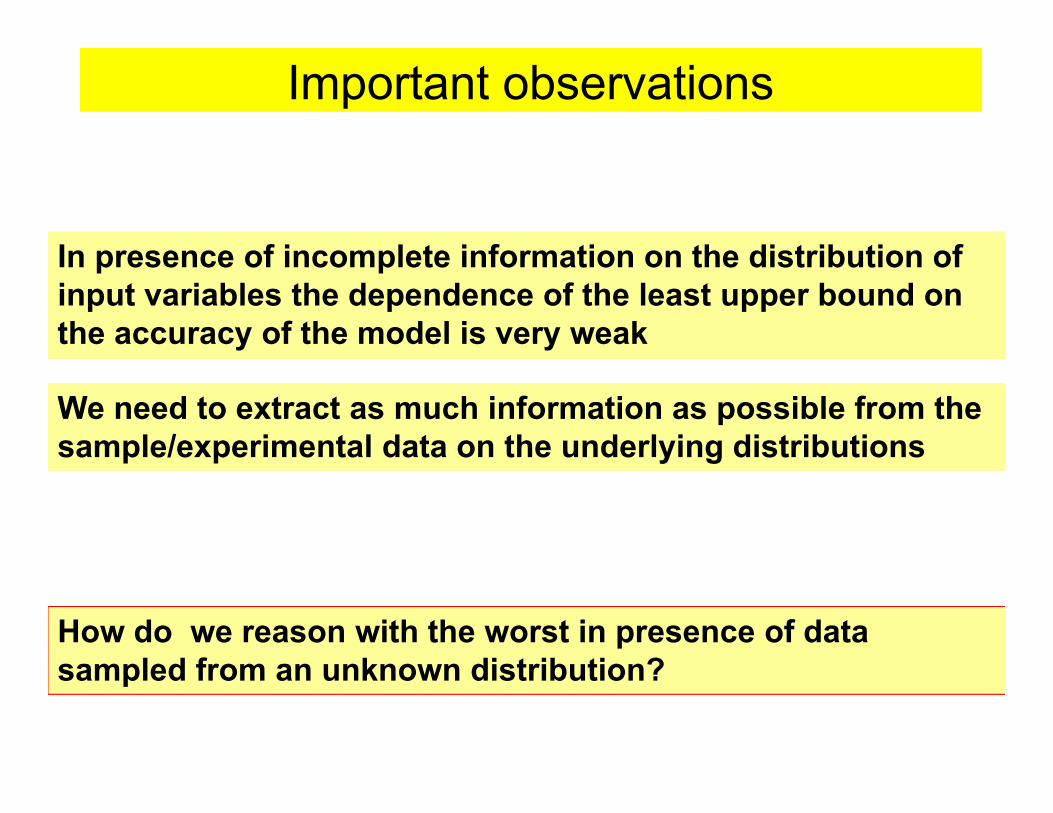
Important observations
In presence of incomplete information on the distribution of input variables the dependence of the least upper bound on the accuracy of the model is very weak
We need to extract as much information as possible from the sample/experimental data on the underlying distributions
How do we reason with the worst in presence of data sampled from an unknown distribution?
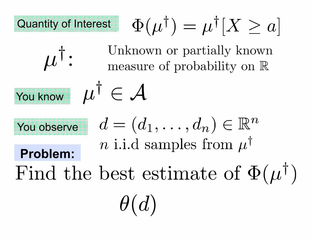
Quantity of Interest
You observe
You know μ† ∈ A
Problem:
θ(d)

Player I Player II
Chooses θ
Mean squared error
Confidence error
Max Min

Game theory and statistical decision theory
John Von Neumann Abraham Wald
J. Von Neumann. Zur Theorie der Gesellschaftsspiele. Math. Ann., 100(1):295–320,1928
J. Von Neumann and O. Morgenstern. Theory of Games and Economic Behavior.Princeton University Press, Princeton, New Jersey, 1944.
A. Wald. Contributions to the theory of statistical estimation and testing hypotheses.Ann. Math. Statist., 10(4):299–326, 1939.
A. Wald. Statistical decision functions which minimize the maximum risk. Ann.of Math. (2), 46:265–280, 1945.
A. Wald. An essentially complete class of admissible decision functions. Ann.Math. Statistics, 18:549–555, 1947.
A. Wald. Statistical decision functions. Ann. Math. Statistics, 20:165–205, 1949.

Player I
Player II
3
1
-2
-2
Deterministic zero sum game
Player I’s payoff
Player I & II both have a blue and a red marbleAt the same time, they show each other a marble
How should I & II play the game?

Pure strategy solution
3
1
-2
-2II should play blue and loose 1 in the worst case
I should play red and loose 2 in the worst case
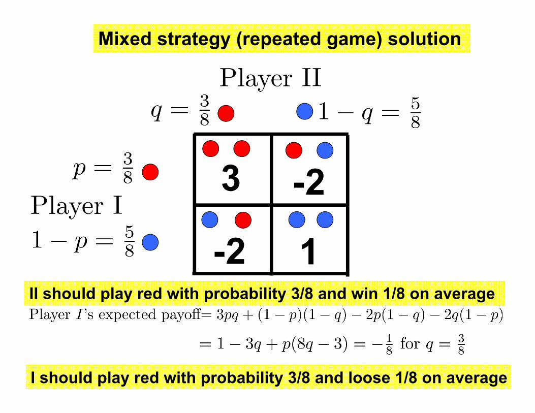
Mixed strategy (repeated game) solution
3
1
-2
-2II should play red with probability 3/8 and win 1/8 on average
I should play red with probability 3/8 and loose 1/8 on average

3
1
-2
-2 Player I’s payoff
J. Von Neumann

Max Min
Optimal bound on the statistical errormaxμ∈A
E(μ, θ)
Optimal statistical estimatorsminθ
maxμ∈A
E(μ, θ)
Pure strategy solution for Player II
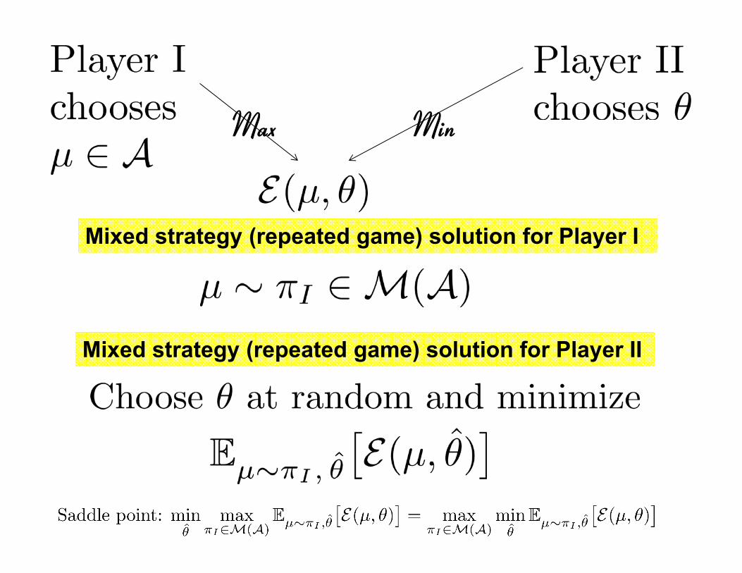
Max Min
Mixed strategy (repeated game) solution for Player II
Mixed strategy (repeated game) solution for Player I

Theorem
Can we have equality?

Theorem
The best mixed strategy for I and II = worst prior for II
A. Dvoretzky, A. Wald, and J. Wolfowitz. Elimination of randomization in certainstatistical decision procedures and zero-sum two-person games. Ann. Math.Statist., 22(1):1–21, 1951.
The best estimator is not random if the loss function is strictly convex

Non Bayesian
Bayesian
Complete class theorem
Risk
Prior
EstimatorNon cooperative Minmax loss/error
cooperative Bayesian loss/error
Over-estimate risk
Under-estimate risk

L. Le Cam. An extension of Wald’s theory of statistical decision functions. Ann.Math. Statist., 26:69–81, 1955
L. J. Savage. The theory of statistical decision. Journal of the American StatisticalAssociation, 46:55–67, 1951.
Further generalization of Statistical decision theory
A. Shapiro and A. Kleywegt. Minimax analysis of stochastic problems. Optim.Methods Softw., 17(3):523–542, 2002.
M. Sniedovich. The art and science of modeling decision-making under severeuncertainty. Decis. Mak. Manuf. Serv., 1(1-2):111–136, 2007
M. Sniedovich. A classical decision theoretic perspective on worst-case analysis.Appl. Math., 56(5):499–509, 2011.
L. D. Brown. Minimaxity, more or less. In Statistical Decision Theory and RelatedTopics V, pages 1–18. Springer, 1994.
L. D. Brown. An essay on statistical decision theory. Journal of the AmericanStatistical Association, 95(452):1277–1281, 2000.
I. Gilboa and D. Schmeidler. Maxmin expected utility with non-unique prior.Journal of Mathematical Economics, 18(2):141–153, 1989

H. Owhadi and C. Scovel. Towards Machine Wald. Handbook for UncertaintyQuantication, 2016. arXiv:1508.02449.
If we want to make decision theory practical for UQ we need to introduce computational complexity constraints
Impact in econometrics and social sciences
R. Leonard. Von Neumann, Morgenstern, and the Creation of Game Theory: FromChess to Social Science, 1900–1960. Cambridge University Press, 2010.
O. Morgenstern. Abraham Wald, 1902-1950. Econometrica: Journal of the Econo-metric Society, pages 361–367, 1951.
G. Tintner. Abraham Wald’s contributions to econometrics. Ann. Math. Statistics,23:21–28, 1952.
How do we do that?
Is there a natural relation between game theory, computational complexity and numerical approximations?

Ax = b
Φx = y
A: Known n× n symmetricpositive definite matrix
b: Unknown element of Rn
Approximate solution x of
Based on the information that
Φ: Known m× nrank m matrix (m < n)
y: Known element of Rm
A simple approximation problem

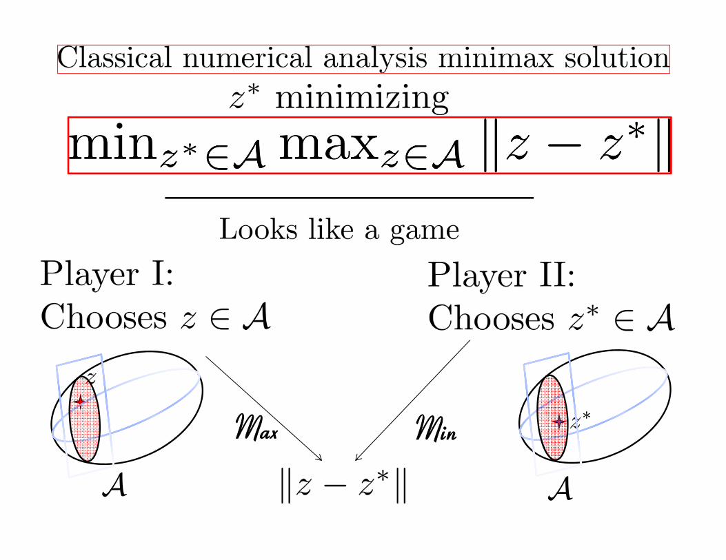
AMax Min
A


Deterministic zero sum game
3
1
-2
-2Player I’s payoff
How should I and II play the game?
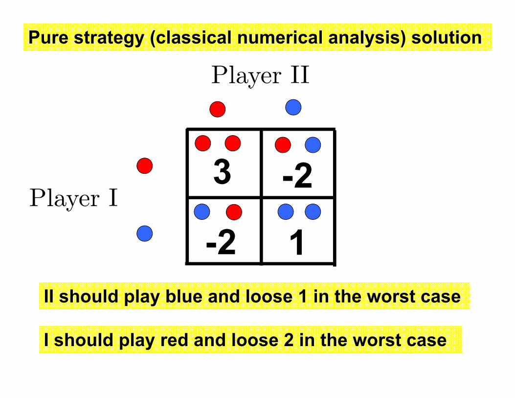
Pure strategy (classical numerical analysis) solution
3
1
-2
-2II should play blue and loose 1 in the worst case
I should play red and loose 2 in the worst case

Mixed strategy (repeated game) solution
3
1
-2
-2II should play red with probability 3/8 and win 1/8 on average
I should play red with probability 3/8 and loose 1/8 on average
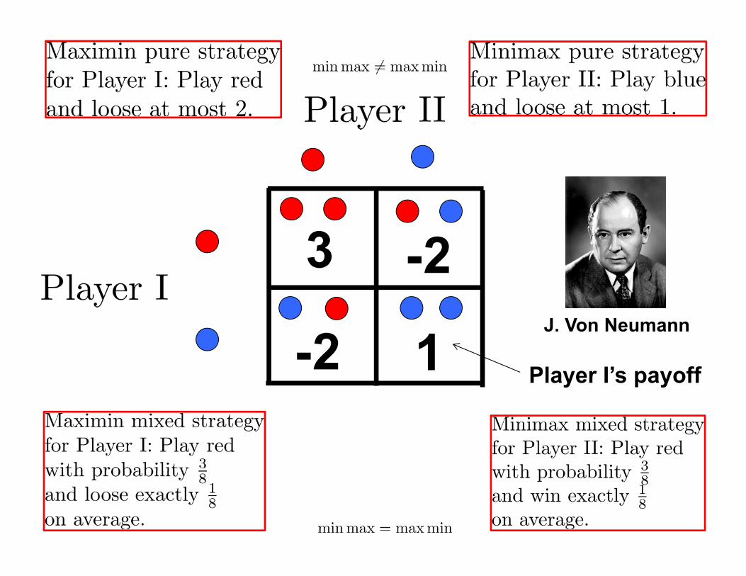
3
1
-2
-2 Player I’s payoff
J. Von Neumann

Game theoretic formulationAx = b
Max Min
Abraham Wald
Continuous game but as in decision theory under compactness it can be approximated by a finite game

Best strategy: lift minimax to measuresAx = b
Max Min
The best strategy for I is to play at randomPlayer II’s best strategy live
in the Bayesian class of estimators

Player II’s mixed strategy
Ax = b AX = ξξ ∼ N (0, Q)
Player II’s bet

Player II’s mixed strategy
Ax = b AX = ξξ ∼ N (0, Q)
Theorem
Owhadi 2015, Multi-grid with rough coefficients and Multiresolution PDE decomposition from Hierarchical Information Games, arXiv:1503.03467, SIAM Review (to appear)

Main Question
Can we turn the process of discovery of a scalable numerical method into a UQ problem and, to some degree, solve it as such in an automated fashion?
Can we use a computer, not only to implement a numerical method but also to find the method itself?
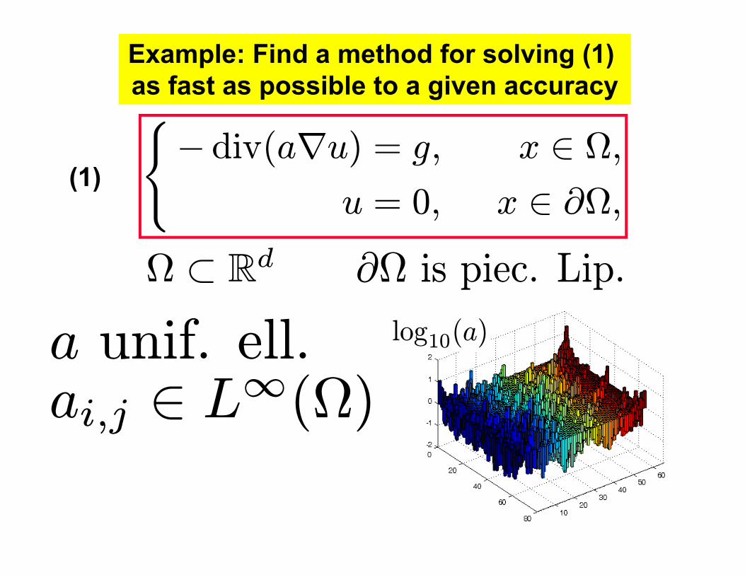
− div(a∇u) = g, x ∈ Ω,u = 0, x ∈ ∂Ω,
(1)
Ω ⊂ Rd ∂Ω is piec. Lip.
a unif. ell.ai,j ∈ L∞(Ω)
Example: Find a method for solving (1) as fast as possible to a given accuracy
log10(a)

Multigrid Methods
Multiresolution/Wavelet based methods[Brewster and Beylkin, 1995, Beylkin and Coult, 1998, Averbuch et al., 1998]
Multigrid: [Fedorenko, 1961, Brandt, 1973, Hackbusch, 1978]
• Linear complexity with smooth coefficients
Severely affected by lack of smoothnessProblem

[Mandel et al., 1999,Wan-Chan-Smith, 1999,Xu and Zikatanov, 2004, Xu and Zhu, 2008], [Ruge-Stuben, 1987]
Robust/Algebraic multigrid
• Some degree of robustness but problem remains open with rough coefficients
Why?Don’t know how to bridge scales with rough coefficients!
Interpolation operators are unknown
[Vassilevski - Wang, 1997, 1998]
Stabilized Hierarchical bases, Multilevel preconditioners
[Panayot - Vassilevski, 1997]
[Chow - Vassilevski, 2003]
[Panayot - 2010]
[Aksoylu- Holst, 2010]

Low Rank Matrix Decomposition methodsFast Multipole Method: [Greengard and Rokhlin, 1987]
Hierarchical Matrix Method: [Hackbusch et al., 2002]
[Bebendorf, 2008]:
N ln2d+8N complexityTo achieve grid-size accuracy in L2-norm

Their process of discovery is based on intuition, brilliant insight, and guesswork
Common theme between these methods
Can we turn this process of discovery into an algorithm?

YESAnswer:
Identify gameFind optimal strategy
N ln3dN complexityResulting method:
Compute fast
This is a theorem
Compute with partial information
Play adversarial Information game
To achieve grid-size accuracy in H1-normSubsequent solves: N lnd+1N complexity
Owhadi 2015, Multi-grid with rough coefficients and Multiresolution PDE decomposition from Hierarchical Information Games, arXiv:1503.03467, SIAM Review (to appear)

Resulting method:
H10 (Ω) = W(1) ⊕aW(2) ⊕a · · ·⊕aW(k) ⊕a · · ·
(− div(a∇u) = g in Ω,
u = 0 on ∂Ω,
For v ∈W(k)
C12k≤ kvka
k div(a∇v)kL2(Ω)≤ C2
2k
Theorem
< ψ,χ >a:=RΩ(∇ψ)Ta∇χ = 0 for (ψ,χ) ∈W(i) ×W(j), i 6= j
kvk2a :=< v, v >a=RΩ(∇v)T a∇v
Looks like an eigenspace decomposition

w(k) = F.E. sol. of PDE in W(k)
Can be computed independently
u = w(1) + w(2) + · · ·+ w(k) + · · ·
u=
w(1) w(2) w(3)
w(4) w(5) w(6)
8× 10⁻³
1.5× 10⁻³ 4× 10⁻⁴ 4× 10⁻⁵
0.030.14
+
+
+
+
Multiresolution decomposition of solution space
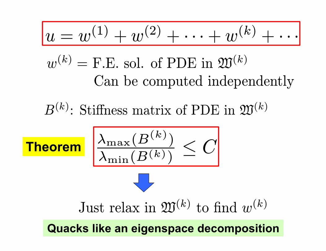
Quacks like an eigenspace decomposition
w(k) = F.E. sol. of PDE in W(k)
Can be computed independently
B(k): Stiffness matrix of PDE in W(k)
Theorem λmax(B(k))
λmin(B(k))≤ C
Just relax in W(k) to find w(k)
u = w(1) + w(2) + · · ·+ w(k) + · · ·

Swims like an eigenspace decomposition
μ(x)∂2t u− div(a∇u) = g(x, t)
Application to time dependent problems
μ(x)∂tu− div(a∇u) = g(x, t)
[Owhadi-Zhang 2016, From gamblets to near FFT-complexitysolvers for wave and parabolic PDEs with rough coefficients]
Hyperbolic and parabolic PDEs with rough coefficientscan be solved in O(N ln3dN) (near FFT) complexity
u=
w(1) w(2) w(3)
w(4) w(5) w(6)
8× 10⁻³
1.5× 10⁻³ 4× 10⁻⁴ 4× 10⁻⁵
0.030.14
+
+
+
+

Doesn’t have the complexity of an eigenspace decomposition
Theorem
Can be performed and stored in
V: F.E. space of H10 (Ω) of dim. N
V = W(1) ⊕aW(2) ⊕a · · ·⊕aW(k)
The decomposition
O(N ln3dN) operations
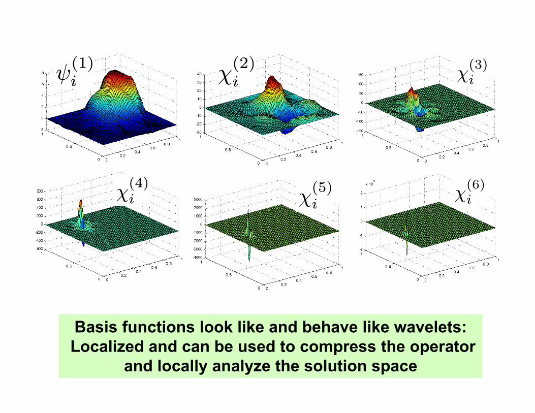
ψ(1)i χ
(2)i χ
(3)i
χ(4)i χ
(5)i
χ(6)i
Basis functions look like and behave like wavelets:Localized and can be used to compress the operator
and locally analyze the solution space

u
H−1(Ω)H10 (Ω)
um gm
div(a∇·)
g
Inverse Problem
Reduced operator
∈ RmRmNumerical implementation requirescomputation with partial information.
um ∈ Rm u ∈ H10 (Ω)Missing information
φ1, . . . ,φm ∈ L2(Ω)
um = (Ωφ1u, . . . , Ω φmu)

Discovery process (− div(a∇u) = g in Ω,
u = 0 on ∂Ω,
φ1, . . . ,φm ∈ L2(Ω)
u− u∗a
Player I Player IIChoosesg ∈ L2(Ω) Sees
Ωuφ1, . . . , Ω uφm
Chooses u∗ ∈ L2(Ω)kgkL2(Ω) ≤ 1
Max Min
Identify underlying information game
Measurement functions:
kfk2a :=RΩ(∇f)T a∇f

Player I
Player II
3
1
-2
-2
Deterministic zero sum game
Player I’s payoff
Player I & II both have a blue and a red marbleAt the same time, they show each other a marble
How should I & II play the (repeated) game?

Game theory
John Von Neumann
John Nash
Player I
Player II
3
1
-2
-2
= 3pq + (1− p)(1− q)− 2p(1− q)− 2q(1− p)=1− 3q + p(8q − 3) =− 1
8 for q = 38
q 1− q
p
1− p
Optimal strategies are mixed strategies
Optimal way toplay is at random
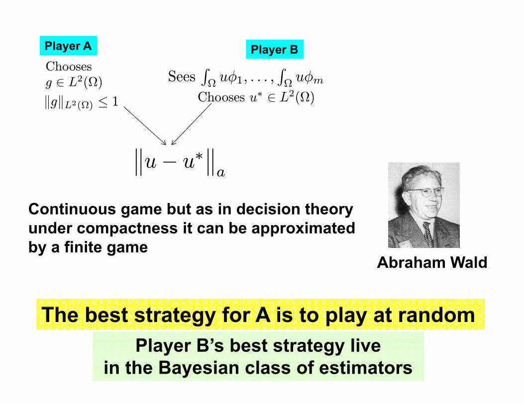
Abraham Wald
The best strategy for A is to play at randomPlayer B’s best strategy live
in the Bayesian class of estimators
Player A Player BChoosesg ∈ L2(Ω) Sees
RΩuφ1, . . . ,
RΩuφm
Chooses u∗ ∈ L2(Ω)kgkL2(Ω) ≤ 1
Continuous game but as in decision theoryunder compactness it can be approximatedby a finite game
°°u− u∗°°a
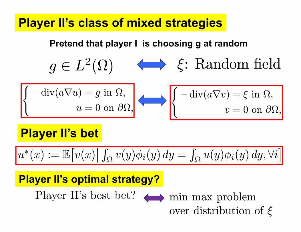
Player II’s class of mixed strategies
(− div(a∇u) = g in Ω,
u = 0 on ∂Ω,
(− div(a∇v) = ξ in Ω,
v = 0 on ∂Ω,
ξ: Random field
u∗(x) := E£v(x)
¯ RΩv(y)φi(y) dy =
RΩu(y)φi(y) dy,∀i
¤Player II’s bet
g ∈ L2(Ω)
Pretend that player I is choosing g at random
min max problemover distribution of ξ
Player II’s optimal strategy?
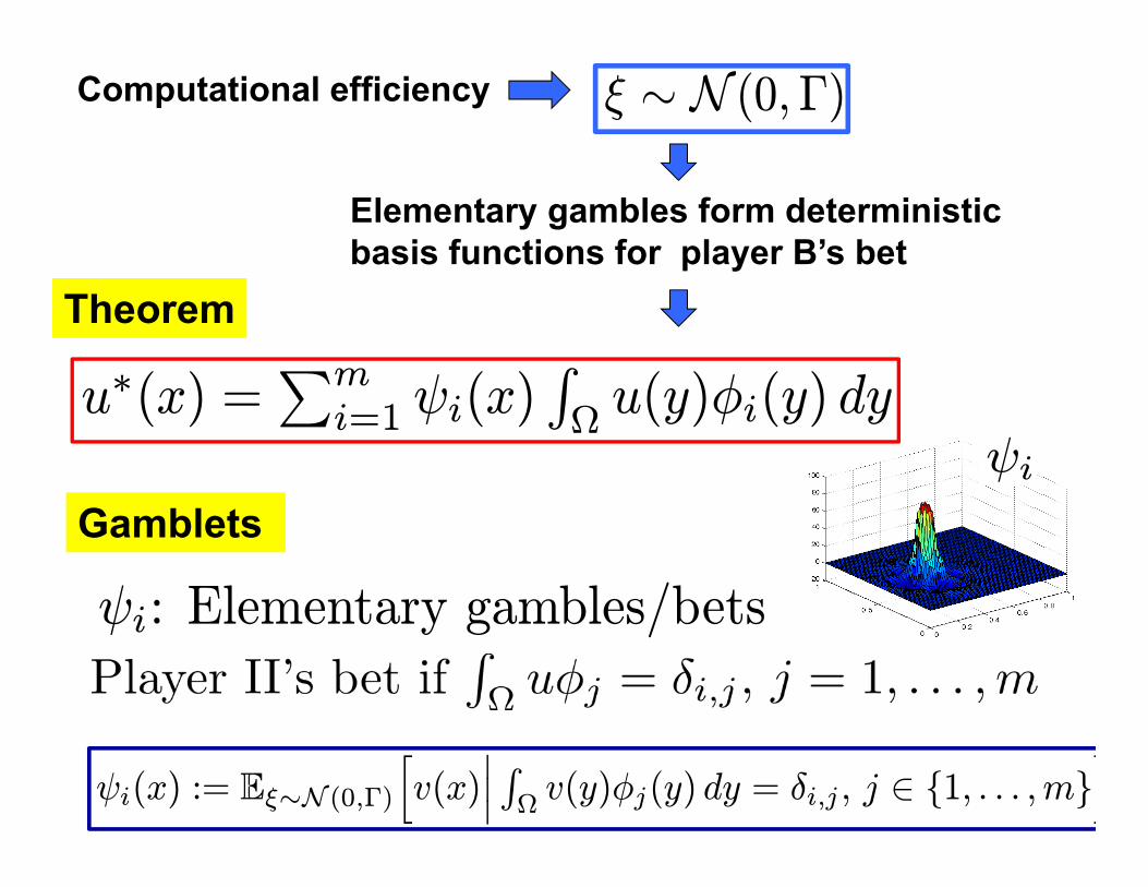
Theorem
ψi(x) := Eξ∼N (0,Γ)hv(x)
¯ RΩv(y)φj(y) dy = δi,j , j ∈ 1, . . . ,m
iψi: Elementary gambles/bets
ψiGamblets
Elementary gambles form deterministic basis functions for player B’s bet
u∗(x) =Pm
i=1 ψi(x)RΩu(y)φi(y) dy
ξ ∼ N (0,Γ)Computational efficiency

Depend onWhat are these gamblets?
Example
Γ(x, y) = δ(x− y)φi(x) = δ(x− xi)
Ω
xi
x1
xm
a = Id ψi: Polyharmonic splines[Harder-Desmarais, 1972][Duchon 1976, 1977,1978]
ai,j ∈ L∞(Ω) ψi: Rough Polyharmonic splines[Owhadi-Zhang-Berlyand 2013]
• Γ: Covariance function of ξ (Player B’s decision)
• (φi)mi=1: Measurements functions (rules of the game)

What is Player II’s best choice for
Γ(x, y) = E£ξ(x)ξ(y)
¤What is Player II’s best strategy?
Γ = LL = − div(a∇·)
RΩξ(x)f(x) dx ∼ N (0, kfk2a)
kfk2a :=RΩ(∇f)Ta∇f
Why? See algebraic generalization
?

Theorem
u∗(x) is the F.E. solution of (1) in spanL−1φi|i = 1, . . . ,mku− u∗ka = infψ∈spanL−1φi:i∈1,...,m ku− ψka
If Γ = L then
The recovery is optimal (Galerkin projection)
L = − div(a∇·)(− div(a∇u) = g, x ∈ Ω,
u = 0, x ∈ ∂Ω,(1)

Theorem ψi: Unique minimizer of(Minimize kψkaSubject to ψ ∈ H1
0 (Ω) andRΩφjψ = δi,j , j = 1, . . . ,m
Pmi=1 wiψi minimizes kψka
over all ψ such thatRΩφjψ = wj for j = 1, . . . ,m
TheoremOptimal variational properties
Variational characterization

Selection of measurement functions
Theorem ku− u∗ka ≤ Hλmin(a)
kgkL2(Ω)
φi = 1τi τi
Ω
diam(τi) ≤ H
τj
Indicator functions of aExample
Partition of Ω of resolution H

Elementary gamble
ψi
(− div(a∇u) = g, x ∈ Ω,
u = 0, x ∈ ∂Ω,(1)
Your best bet on the value of u
τi
Ωτj
10000
0000
0000
0
00
given the information thatRτiu = 1 and
Rτju = 0 for j 6= i

Exponential decay of gamblets
TheoremRΩ∩(B(τi,r))c(∇ψi)
Ta∇ψi ≤ e−rlH kψik2a
x-axis slice
ψi
ψi
log10¡10−10 + |ψi||
¢x-axis slice
4
−10
r
Ω
τi

r
Ω
τiSr
Theorem
ku− u∗,locka ≤ 1√λmin(a)
HkgkL2(Ω)
u∗,loc(x) =Pm
i=1 ψloc,ri (x)
RΩu(y)φi(y) dy
If r ≥ CH ln 1H
No loss of accuracy iflocalization ∼ H ln 1
H
ψloc,ri : Minimizer of(Minimize kψkaSubject to ψ ∈ H1
0 (Sr) andRSr
φjψ = δi,j
for τj ∈ Sr
Localization of the computation of gamblets

Formulation of the hierarchical game

Hierarchy of nested Measurement functions
φ(1)2 = 1
τ(1)2
φ(2)2,3 = 1
τ(2)2,3
φ(k)i1,...,ik
with k ∈ 1, . . . , qφ(k)i =
Pj ci,jφ
(k+1)i,j
τ(1)2 τ
(2)2,3
τ(3)2,3,1
φ(3)2,3,1 = 1
τ(3)2,3,1
Example
φ(1)i1
φ(2)i1,j1
φ(2)i1,j2
φ(2)i1,j3
φ(2)i1,j4
φ(3)i1,j2,k1
φ(3)i1,j2,k2
φ(3)i1,j2,k3
φ(3)i1,j2,k4
φ(k)i : Indicator functions of a
hierarchical nested partition of Ω of resolution Hk = 2−k

iΠ1,2i
I1 I2 I3
j ∈ Π1,2i ⊂ Π2I Π2,3j
Π1,3i
τ(1)i τ
(2)j
φ(1)i φ
(2)i φ
(3)i
φ(4)i φ
(5)i φ
(6)i
In the discrete setting simply aggregate elements(as in algebraic multigrid)

Player I Player IIChoosesg ∈ L2(Ω)
Formulation of the hierarchy of games
kgkL2(Ω) ≤ 1
(− div(a∇u) = g in Ω,
u = 0 on ∂Ω,
Must predict
Sees Ωuφ
(k)i , i ∈ Ik
u and Ωuφ
(k+1)j , j ∈ Ik+1
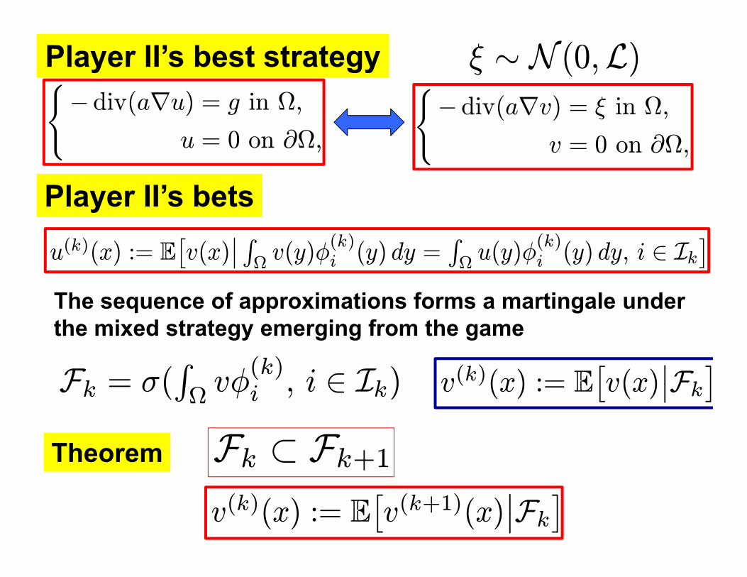
Player II’s best strategy(− div(a∇u) = g in Ω,
u = 0 on ∂Ω,
(− div(a∇v) = ξ in Ω,
v = 0 on ∂Ω,
ξ ∼ N (0,L)
u(k)(x) := E£v(x)
¯ RΩv(y)φ
(k)i (y) dy =
RΩu(y)φ
(k)i (y) dy, i ∈ Ik
¤Player II’s bets
Fk = σ(RΩvφ
(k)i , i ∈ Ik) v(k)(x) := E
£v(x)
¯Fk¤
Theorem Fk ⊂ Fk+1v(k)(x) := E
£v(k+1)(x)
¯Fk¤
The sequence of approximations forms a martingale under the mixed strategy emerging from the game

Player II’s best strategy(− div(a∇u) = g in Ω,
u = 0 on ∂Ω,
(− div(a∇v) = ξ in Ω,
v = 0 on ∂Ω,
ξ ∼ N (0,L)
u(k)(x) := E£v(x)
¯ RΩv(y)φ
(k)i (y) dy =
RΩu(y)φ
(k)i (y) dy, i ∈ Ik
¤Player II’s bets
u(1) u(2) u(3)
u(4) u(5) u(6)

Gamblets Elementary gambles form a hierarchy of deterministic basis functions for player II’s hierarchy of bets
Theorem u(k)(x) =P
i ψ(k)i (x)
RΩu(y)φ
(k)i (y) dy
ψ(k)i : Elementary gambles/bets at resolution Hk = 2−k
ψ(k)i (x) := E
hv(x)
¯ RΩv(y)φ
(k)j (y) dy = δi,j , j ∈ Ik
iψ(1)i ψ
(2)i ψ
(3)i
ψ(4)i ψ
(5)i ψ
(6)i

Theorem
V(k) ⊂ V(k+1)
V(k) := spanψ(k)i , i ∈ Ik ψ(1)i1
ψ(2)i1,j1
ψ(2)i1,j2
ψ(2)i1,j3
ψ(2)i1,j4
ψ(3)i1,j2,k1
ψ(3)i1,j2,k2
ψ(3)i1,j2,k3
ψ(3)i1,j2,k4
Gamblets are nested
ψ(k)i (x) =
Pj∈Ik+1 R
(k)i,j ψ
(k+1)j (x)

R(k)i,j = E
£ RΩv(y)φ
(k+1)j (y) dy
¯ RΩv(y)φ
(k)l (y) dy = δi,l, l ∈ Ik
¤Interpolation/Prolongation operator
10 0
0
R(k)i,j
Your best bet on the value ofRτ(k+1)j
u
given the information thatRτ(k)iu = 1 and
Rτlu = 0 for l 6= i
τ(k)i R
(k)i,j
τ(k+1)j

At this stage you can finish withclassical multigrid
But we want multiresolution decomposition

Elementary gamble
Ω
00
0
χ(k)i
000
00τ
(k)i τ
(k)j
00
00
Your best bet on the value of u
given the information thatRτ(k)i
u = 1,Rτ(k)
i−u = −1 and
Rτ(k)j
u = 0 for j 6= i
100
-1
τ(k)i−

+1−1
χ(k)i = ψ
(k)i − ψ
(k)i−
+1
−1
+1−1
i = (i1, . . . , ik−1, ik)
i− = (i1, . . . , ik−1, ik − 1)
ψ(1)i1
ψ(2)i1,j1
ψ(2)i1,j2
ψ(2)i1,j3
ψ(2)i1,j4
+1−1
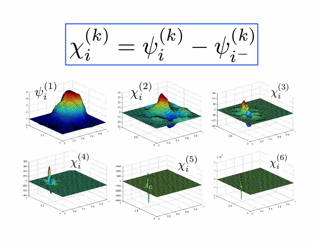
ψ(1)i χ
(2)i χ
(3)i
χ(4)i χ
(5)i
χ(6)i
χ(k)i = ψ
(k)i − ψ
(k)i−

Theorem
W(k+1): Orthogonal complement of V(k) in V(k+1)
with respect to < ψ,χ >a:=RΩ(∇ψ)T a∇χ
H10 (Ω) = V(1) ⊕aW(2) ⊕a · · ·⊕aW(k) ⊕a · · ·
Multiresolution decomposition of the solution space
V(k) := spanψ(k)i , i ∈ IkW(k) := spanχ(k)i , i

Theorem
u(k+1) − u(k) = F.E. sol. of PDE in W(k+1)
u=
u(1) u(2) − u(1) u(3) − u(2)
u(4) − u(3) u(5) − u(4) u(6) − u(5)
8× 10⁻³
1.5× 10⁻³ 4× 10⁻⁴ 4× 10⁻⁵
0.030.14
+
+
+
+
Multiresolution decomposition of the solution
Subband solutions u(k+1) − u(k)can be computed independently

Uniformly bounded condition numbers
A(k)i,j :=
ψ(k)i ,ψ
(k)j
®a
B(k)i,j :=
χ(k)i ,χ
(k)j
®a
4.5log10(
λmax(A(k))
λmin(A(k)))
log10(λmax(B
(k))λmin(B(k))
)
Theoremλmax(B
(k))
λmin(B(k))≤ C
Just relax!In v ∈W(k)
to getu(k) − u(k−1)

V = W(1) ⊕aW(2) ⊕a · · ·⊕aW(k)
Ranges of eigenvalues in V andW(k) (k = 1, . . . , 5) in log scale
£infψ∈V
kψk2akψk2
L2, supψ∈V
kψk2akψk2
L2
¤
£infψ∈W(k)
kψk2akψk2
L2, supψ∈W(k)
kψk2akψk2
L2
¤

c(1)i
c(2)j
c(3)j
c(4)j
0 200 400 600 800-6
-4
-2
0
2
4x 10
-4
c(5)j c
(6)j
u =P
i c(1)i
ψ(1)i
kψ(1)i ka+Pq
k=2
Pj c(k)j
χ(k)j
kχ(k)j ka
0 1000 2000 3000 4000-4
-2
0
2
4x 10
-5
Coefficients of the solution in the gamblet basis
c(6)j

Operator Compression
Throw 99% of the coefficients
u
Gamblets behave like wavelets but they are adapted to the PDE and can compress its solution space
Gamblet compression
Compression ratio = 105Energy norm relative error = 0.07
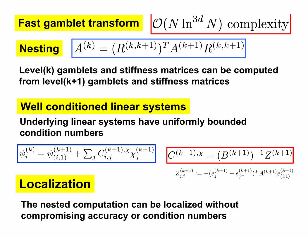
Fast gamblet transform
Nesting A(k) = (R(k,k+1))TA(k+1)R(k,k+1)
Level(k) gamblets and stiffness matrices can be computedfrom level(k+1) gamblets and stiffness matrices
Well conditioned linear systems
ψ(k)i = ψ
(k+1)(i,1) +
Pj C
(k+1),χi,j χ
(k+1)j C(k+1),χ = (B(k+1))−1Z(k+1)
LocalizationZ(k+1)j,i := −(e
(k+1)j − e(k+1)j− )TA(k+1)e
(k+1)(i,1)
Underlying linear systems have uniformly bounded condition numbers
The nested computation can be localized without compromising accuracy or condition numbers
O(N ln3dN) complexity

Theorem
Localizing (ψ(k)i )i∈Ik and (χ
(k)i )i to subdomains of size
≥ CHk ln 1Hk
≥ CHk(ln 1Hk
+ ln 1² )
Cond. No (B(k),loc) ≤ C
°°u− u(1),loc −Pq−1k=1(u
(k+1),loc − u(k),loc)°°a≤ ²
The number of operations to compute gamblets andachieve accuracy ² is O
¡N ln3d
¡max( 1
², N1/d)
¢¢(and O
¡N lnd(N1/d) ln 1
²
¢for subsequent solves)
Theorem
Complexity
O(N ln3dN) O(N lnd+1N)GambletTransform
LinearSolve

u(3) − u(2)8× 10⁻³
u(2) − u(1)0.03
u(1)0.14
...
u(1)
ϕi, Ah,Mh χ
(q)i , B
(q)ψ(q)i , A(q) u(q) − u(q−1)
ψ(q−1)i , A(q−1) χ
(q−1)i , B(q−1) u(q−1) − u(q−2).
..
...
χ(3)i , B(3)ψ
(3)i , A(3) u(3) − u(2)
ψ(2)i , A(2) χ
(2)i , B(2) u(2) − u(1)
ψ(1)i , A(1)
ψ(1)i
χ(2)i
χ(3)i
ψ(1)i
ψ(2)i
ψ(3)i
Parallel operatingdiagram
both in space and in
frequency

Numerical Homogenization
HMM
Harmonic Coordinates
[Gloria 2010]
Babuska, Caloz, Osborn, 1994Allaire Brizzi 2005; Owhadi, Zhang 2005
Engquist, E, Abdulle, Runborg, Schwab, et Al. 2003-...
MsFEM [Hou, Wu: 1997]; [Efendiev, Hou, Wu: 1999]
Nolen, Papanicolaou, Pironneau, 2008
[Chu-Graham-Hou-2010] (limited inclusions)
[Babuska-Lipton 2010] (local boundary eigenvectors)[Efendiev-Galvis-Wu-2010] (limited inclusions or mask)
[Malqvist-Peterseim 2012] Volume averaged interpolation
Flux norm Berlyand, Owhadi 2010; Symes 2012
Arbogast, 2011: Mixed MsFEM
Kozlov, 1979
Localization
[Fish - Wagiman, 1993]
Projection based method
[Owhadi-Zhang 2011] (localized transfer property)

Statistical approach to numerical approximation

Statistical approach to numerical approximation

Some high level remarks

What is the worst?
Au†: Unknown element of A
Robust Optimization worst case
Φ : A −→ Ru −→ Φ(u) Quantity of Interest
What is Φ(u†)?
infu∈AΦ(u) ≤ Φ(u†) ≤ supu∈A Φ(u)

A
Game theoretic worst case
AMax Min

Confidence error
Robust Optimization worst caseFailure is not an option. You want to always be right.
Game theoretic worst case
Interpretation depends on the choice of loss function.
You want to be right with high probability.
Quadratic errorYou want to be right on average.Well suited for numerical computation where you need to keep computing with partial information (e.g. invert a 1,000,000 by 1,000,000 matrix)

Non Bayesian
Bayesian
Complete class theorem
Risk
Prior
EstimatorNon cooperative Minmax loss/error
cooperative Bayesian loss/error
Over-estimate risk
Under-estimate risk
Can we approximate the optimal prior?

Numerical robustness of Bayesian inference
Can we numerically approximate the prior when closed form expressions are not available for posterior values?


• Brittleness of Bayesian Inference under Finite Information in a Continuous World. H. Owhadi, C. Scovel and T. Sullivan. Electronic Journal of Statistics, vol 9, pp 1-79, 2015. arXiv:1304.6772
• Brittleness of Bayesian inference and new Selberg formulas. H. Owhadi and C. Scovel. Communications in Mathematical Sciences (2015). arXiv:1304.7046
• On the Brittleness of Bayesian Inference. H. Owhadi, C. Scovel and T. Sullivan. SIAM Review, 57(4), 566-582, 2015, arXiv:1308.6306
• Qualitative Robustness in Bayesian Inference (2015). H. Owhadi and C. Scovel. arXiv:1411.3984
Positive Negative• Classical Bernstein Von Mises• Wasserman, Lavine, Wolpert (1993)• P Gustafson & L Wasserman (1995)• Castillo and Rousseau (2013)• Castillo and Nickl (2013)• Stuart & Al (2010+). • ….
• Freedman (1963, 1965)• P Gustafson & L Wasserman (1995)• Diaconis & Freedman 1998• Johnstone 2010• Leahu 2011• Belot 2013
Robustness of Bayesian conditioning in continuous spaces

10.000 children are given one pound of play-doh. On average, how much mass can they put above awhile, on average, keeping the seesaw balanced around m?
Paul is given one pound of play-doh. What can you say about how much mass he isputting above a if all you have is the belief thathe is keeping the seesaw balanced around m?
Brittleness of Bayesian Inference under Finite Information in a Continuous World. H. Owhadi, C. Scovel and T. Sullivan. Electronic Journal of Statistics, vol 9, pp 1-79, 2015. arXiv:1304.6772

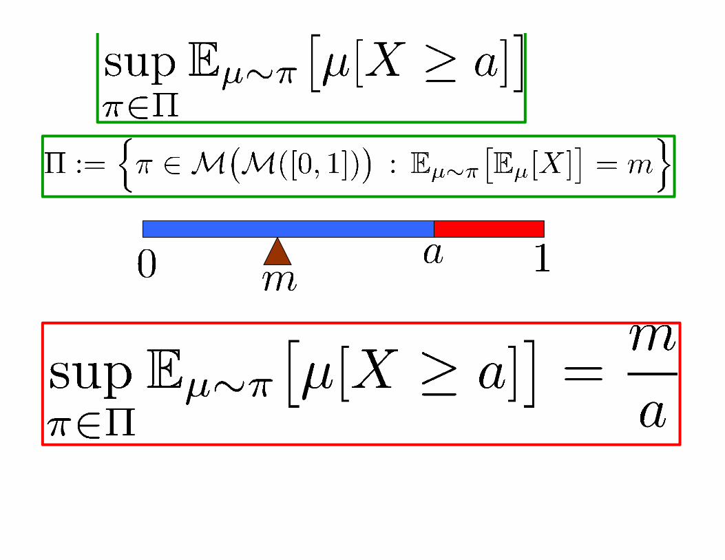
What is the least upper bound on
If all you know is ?
Answer
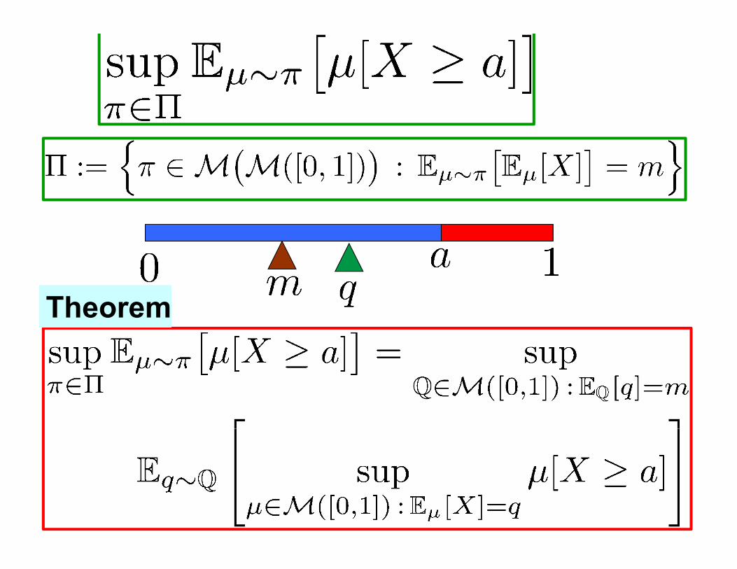
Theorem


Reduction calculus with measures over measures
QΨ
QΨ−1 ⊂M(Q)M(A) ⊃Theorem
supπ∈Ψ−1Q
Eμ∼π Φ(μ)
supQ∈Q
hEq∼Q
£sup
μ∈Ψ−1(q)Φ(μ)
¤i=
M(X ) ⊃ Polishspace
Brittleness of Bayesian Inference under Finite Information in a Continuous World. H. Owhadi, C. Scovel and T. Sullivan. Electronic Journal of Statistics, vol 9, pp 1-79, 2015. arXiv:1304.6772

What is the worst with random data? A
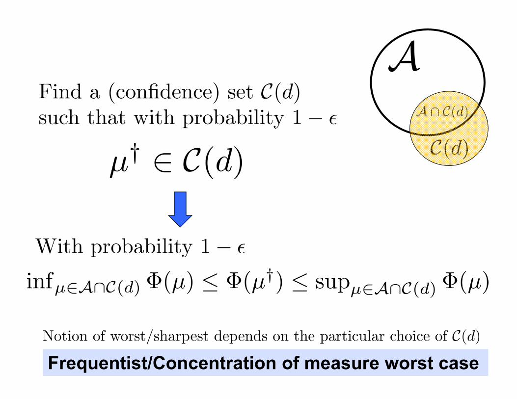
A
Frequentist/Concentration of measure worst case

Theorem
N. Fournier and A. Guillin, On the rate of convergence in Wasserstein distance of the empirical measure, Probability Theory and Related Fields, (2014), pp. 1-32.
A

The extreme points of the Prokhorov, Monge-Wasserstein and Kantorovich metric balls about a measure whose support has at most n points, consist of measures whose supports have at most n+2 points.
• D. Wozabal. A framework for optimization under ambiguity. Annals of Operations Research, 193(1):21—47, 2012.
• P. M. Esfahani and D. Kuhn. Data-driven distributionally robust optimization using the Wasserstein metric: performance guarantees and tractable reformulations. arXiv:1505.05116, 2015.
• Extreme points of a ball about a measure with finite support (2015). H. Owhadi and Clint Scovel. arXiv:1504.06745
Reduction calculus of the ball about the empirical distribution

QuestionGame/Decision Theory + Information Based Complexity
Turn the process of discovery of scalable numerical solversinto an algorithm
Worst case calculus
?
P. L. Chebyshev1821-1894
M. G. Krein1907-1989
A. A. Markov1856-1922
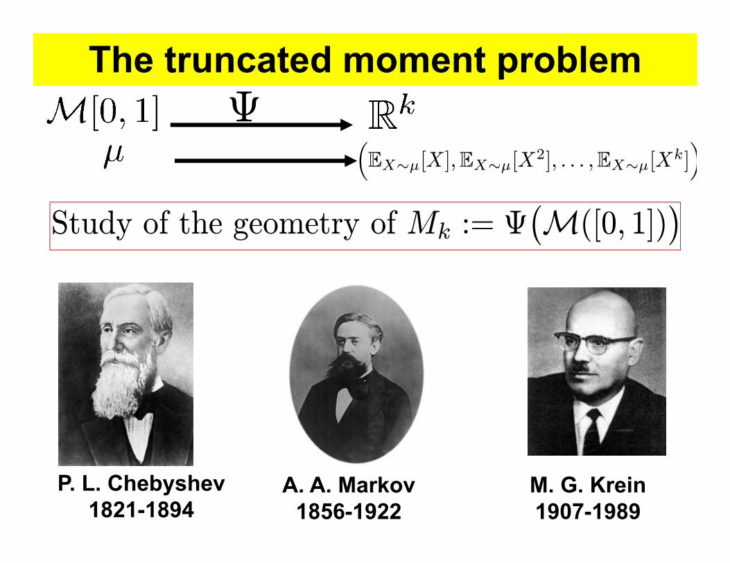
The truncated moment problem
³EX∼μ[X],EX∼μ[X2], . . . ,EX∼μ[Xk]
´Ψ
Study of the geometry of Mk := Ψ¡M([0, 1])
¢

Finite dim.Infinite dim.
³EX∼μ[X],EX∼μ[X2], . . . ,EX∼μ[Xk]
´Ψ Mk := Ψ¡M([0, 1])
¢
Finite dim.

Finite dim.Infinite dim.
Ψ
t1 t2 tj tN
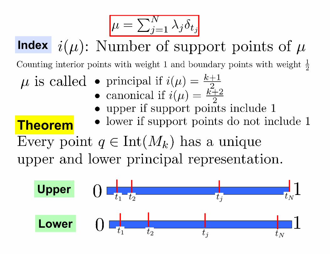
Index
Theorem
t1 t2 tj tN
t1 t2 tj tN
Upper
Lower

Sn(α,β, γ) =Qn−1j=0
Γ(α+jγ)Γ(β+jγ)Γ(1+(j+1)γ)Γ(α+β+(n+j−1)γ)Γ(1+γ)
Selberg Identities
Sn(α,β, γ) :=R[0,1]n
Qnj=1 t
α−1j (1− tj)β−1|∆(t)|2γdt .
∆(t) :=Qj<k (tk − tj)
Brittleness of Bayesian inference and new Selberg formulas. H. Owhadi and C. Scovel. Communications in Mathematical Sciences (2015). arXiv:1304.7046

Forrester and Warnaar 2008
The importance of the Selberg integral
Used to prove outstanding conjectures inRandom matrix theory and cases of the Macdonald conjectures
Central role in random matrix theory, Calogero-Sutherland quantum many-body systems, Knizhnik-Zamolodchikov equations, and multivariable orthogonal polynomial theory

Index
Theorem
t1 t2 tj tNt∗

New Reproducing Kernel Hilbert Spaces and Selberg Integral formulas related to the Markov-Krein representations of moment spaces.
Ψ ³EX∼μ[X],EX∼μ[X2], . . . ,EX∼μ[Xk]
´RImΣt−1 ·Qm
j=1 t2j (1− tj)2∆4m(t)dt = Sm(5,1,2)−Sm(3,3,2)
2RImΣt−1 ·Qm
j=1 t2j ·∆4m(t)dt = m
2 Sm−1(5, 3, 2)
Sn(α,β, γ) =Qn−1j=0
Γ(α+jγ)Γ(β+jγ)Γ(1+(j+1)γ)Γ(α+β+(n+j−1)γ)Γ(1+γ)
∆m(t) :=Qj<k (tk − tj)¡
Σφ¢(t) :=
Pmj=1 φ(tj), t ∈ Im
I := [0, 1]

ZIm−1
hk(t)ΣQj(t)
m−1Yj0=1
t2j0 ·∆4m−1(t)dt = V ol(M2m−1)(2m−1)!(m−1)!(k + 2)!
(8k + 4)(k − 2)!δjk .
Theorem
ej(t) :=X
i1<···<ijti1 · · · tij
Πn0 : n-th degree polynomials which vanish on the boundary of [0, 1]Mn ⊂ Rn: set of q = (q1, . . . , qn) ∈ Rn such that there exists a probabilitymeasure μ on [0, 1] with Eμ[Xi] = qi with i ∈ 1, . . . , n.
Consider the basis of Π2m−10 consisting of the associated Legendre polyno-mials Qj , j = 2, .., 2m − 1 of order 2 translated to the unit interval I. Fork = 2, .., 2m− 1 define
ajk :=(j + k + k2)Γ(j + 2)Γ(j)
Γ(j + k + 2)Γ(j − k + 1), k ≤ j ≤ 2m− 1
hk(t) :=2m−1Xj=k
(−1)j+1ajke2m−1−j(t, t) .
Then for j = k mod 2, j, k = 2, .., 2m− 1, we have
Bi-orthogonal systems of Selberg Integral formulas

Collaborators
Research supported by Air Force Office of Scientific Research
U.S. Department of Energy Office of Science, Office of Advanced Scientific Computing Research, through the Exascale Co-Design Center for Materials in Extreme Environments
National Nuclear Security Administration
Clint Scovel (Caltech), Tim Sullivan (Warwick), Mike McKerns (Caltech), Michael Ortiz (Caltech), Lei Zhang (Jiaotong), Leonid Berlyand (PSU), Lan HuongNguyen, Paul Herve Tamogoue Kamga.
DARPA EQUiPS Program (Enabling Quantification of Uncertainty in Physical Systems)