HiSeq Analysis Software v2.1 User Guide€¦ · HiSeq Analysis Software v2.1 User Guide....

Customize a short end-to-end work�ow guide with the Custom Protocol Selectorsupport.illumina.com/custom-protocol-selector.html

For Research Use Only. Not for use in diagnostic procedures.

January 2017

Document # 15070536 v01

ILLUMINA PROPRIETARY

HiSeq Analysis Software v2.1User Guide

HiSeq Analysis Software v2.1Software Guide

Introduction 3ComputingRequirements 3InstallHiSeq AnalysisSoftware Docker Image 4Run HiSeq AnalysisSoftware in Docker with Open Grid Scheduler 4GenerateFASTQ Workflow 5ResequencingAnalysisWorkflow 9Tumor-NormalAnalysisWorkflow 15Input Files 19Methods for the ResequencingWorkflow 21Methods for Tumor-NormalWorkflow 35Revision History 41TechnicalAssistance 43

Document # 15070536 v01

For Research Use Only. Not for use in diagnostic procedures.1

HiSeqAnalysis Software v2.1 SoftwareGuide

This document and its contents are proprietary to Illumina, Inc. and its affiliates ("Illumina"), and are intended solely for thecontractual use of its customer in connection with the use of the product(s) described herein and for no other purpose. Thisdocument and its contents shall not be used or distributed for any other purpose and/or otherwise communicated, disclosed, orreproduced in any way whatsoever without the prior written consent of Illumina. Illumina does not convey any license under itspatent, trademark, copyright, or common-law rights nor similar rights of any third parties by this document.

The instructions in this document must be strictly and explicitly followed by qualified and properly trained personnel in order toensure the proper and safe use of the product(s) described herein. All of the contents of this document must be fully read andunderstood prior to using such product(s).

FAILURE TO COMPLETELY READ AND EXPLICITLY FOLLOW ALL OF THE INSTRUCTIONS CONTAINED HEREIN MAY RESULTIN DAMAGE TO THE PRODUCT(S), INJURY TO PERSONS, INCLUDING TO USERS OR OTHERS, AND DAMAGE TO OTHERPROPERTY.

ILLUMINA DOES NOT ASSUME ANY LIABILITY ARISING OUT OF THE IMPROPER USE OF THE PRODUCT(S) DESCRIBEDHEREIN (INCLUDING PARTS THEREOF OR SOFTWARE).

© 2017 Illumina, Inc. All rights reserved.

Illumina, HiSeq, the pumpkin orange color, and the streaming bases design are trademarks of Illumina, Inc. and/or its affiliate(s) inthe U.S. and/or other countries. All other names, logos, and other trademarks are the property of their respective owners.

Document # 15070536 v01



IntroductionHiSeq AnalysisSoftware v2.1 isa software package for analyzingsequencingdata generated by Illumina HiSeq Xsequencingsystems. The software leveragesa suite ofproven algorithms todetect genomic variantscomprehensivelyand accurately. HiSeq AnalysisSoftware v2.1 isa complete package with a range of variants, includingSingleNucleotide Variants (SNV), Indels, StructuralVariants (SV) and Copy Number Variants (CNV) for tumor and normalsamples. HiSeq AnalysisSoftware v2.1utilizes the base calls and quality scoresgenerated by Real-Time Analysis(RTA) software during the sequencing run to rapidly handle data for high-throughput whole-genome sequencinganalysis.

HiSeq AnalysisSoftware v2.1uses the Isaac Aligner and Strelka Germline Variant Caller toprovide both aligned andunaligned readsand variants. See Isaac Aligner on page 21and Strelka Germline Variant Caller on page 22 for moreinformation.

For structural variants, HiSeq AnalysisSoftware v2.1uses2complementary approaches:

u Read depth analysisby Canvas. See Canvason page 29.

u Discordant paired-end analysisby Manta. See Manta (StructuralVariant Caller) on page 33.

HiSeq AnalysisSoftware v2.1supportsa multistep analysisworkflow that usesa simple command line andrecommended default settingsspecified in the sample sheet.

Thisdocument providesan overview of the HiSeq AnalysisSoftware v2.1workflow, data structure, computingrequirements, and installation guidelines. The aim of thisdocument is tohelp you understand the details and use ofHiSeq AnalysisSoftware v2.1 for high-throughput whole-genome sequencinganalysis.

Computing Requirements

Operating SystemHiSeq AnalysisSoftware v2.1 requires the CentOS6operatingsystem with docker v1.62or later. To run docker onCentOS-6.5or later, kernel2.6.32-431or higher is required.

To install docker on CentOS6, enter the followingcommands:yum -y install epel-releaseyum -y install docker-io

Compute HardwareHiSeq AnalysisSoftware v2.1 requiresspecific compute architecture for proper functionality and performance. Thehardware required isavailable from a range ofsuppliersand manufacturers.

For a HiSeq X Ten system, the followingarchitecture is recommended for analysis. Archival storage isnot included inthis recommendation.

u Resilient NASsolution servingCIFSand NFSu Aminimum of100TB usable storage capacity with performance > 2GB/s

To retain data after analysis, additional capacity isneeded.u Multiple 10GB or 40GB network links

u Resilient 10GB network

u 26servers, each with the following:u Dual10Core CPUs@ 2.8GHzu 128GB 1867MHz memoryu 6TB usable local storage capacity with performance > 500MB/s

Document # 15070536 v01



u 10GB Ethernet adapter

Install HiSeq Analysis Software Docker ImageToperform installation and extract the reference genome, you need root privileges.

1 Download the following from the link provided by Illumina.u isis-2.6.53.23.tar md5sum 3cb4dbc3853bd8a856b2b84c0dc6cec6u hg38-NSv4.2.tgz md5sum 435cdc86c8ec31135f0e7443f9344e70u hg19-NSv md5sum a08c2f68a3c6a90cb0d3cd0cf713c162

2 Install the analysis software:cat isis-2.6.53.23.tar|docker load

Verify the installation:sudo docker images

3 Extract the hg19and hg38 reference genomes:tar -zxvf hg19-NSv4.2.tgz -C /genometar -zxvf hg38-NSv4.2.tgz -C /genome

When runningHiSeq AnalysisSoftware on a cluster, create a script with the necessary command linesand schedulethe script on a node. See your scheduler documentation for the correct command.

Make sure that the node isdedicated to the script. When running, HiSeq AnalysisSoftware usesall the RAM andcoreson the node.

To run sudodocker, a password isnot needed.sudo visudoUSERNAME ALL = NOPASSWD:/

To run docker without sudo, create a docker group and run the docker daemon aspart of that group. Then add allHiSeq AnalysisSoftware users to the group.

Run HiSeq Analysis Software in Docker with Open Grid SchedulerSince the docker command to run HiSeq AnalysisSoftware doesnot specify the number ofcoresor amount ofmemory that the analysis is limited to, the analysisuses the entire node and allRAM available. With a parallelenvironment, the analysis is sent toonly 1node. The analysis fully occupies that node toprevent another job from usingthe node and oversubscribing that node. For an example ofa threaded parallel environment, see the Oracle entryConfiguringa New ParallelEnvironment.

Use Open Grid Scheduler tocreate a parallel environment. The followingcommand assumes that docker can be runwithout sudo.

NOTE:

The command specifies20corespernode. If youenter> 20cores, the job doesnot run. If youenter< 20cores,there isa risk that other jobsuse the same node and oversubscribe that node.

qsub -pe threaded 20 -cwd -b y -V /path_to_runhas.sh/runhas.sh

Whererunhas.sh is#!/bin/sh# each node may not have isis-2.6.53.23 images loaded.cat /PATH_2_HAS_TAR/isis-2.6.53.23.tar|docker loaddocker run -i \-v /etc/localtime:/etc/localtime:ro \

Document # 15070536 v01



https://blogs.oracle.com/templedf/entry/configuring_a_new_parallel_environment

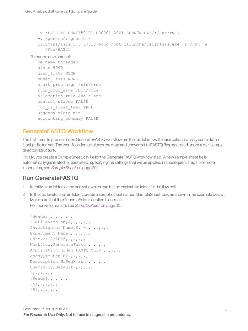
-v /PATH_TO_RUN/150101_E00001_0001_AHNN7NCCXX/:/Run:rw \-v /genome/:/genome \illumina/isis:2.6.53.23 mono /opt/illumina/Isis/Isis.exe -r /Run -a

/Run/HAS21

Threaded environment:pe_name threadedslots 9999user_lists NONExuser_lists NONEstart_proc_args /bin/truestop_proc_args /bin/trueallocation_rule $pe_slotscontrol_slaves FALSEjob_is_first_task TRUEurgency_slots minaccounting_summary FALSE

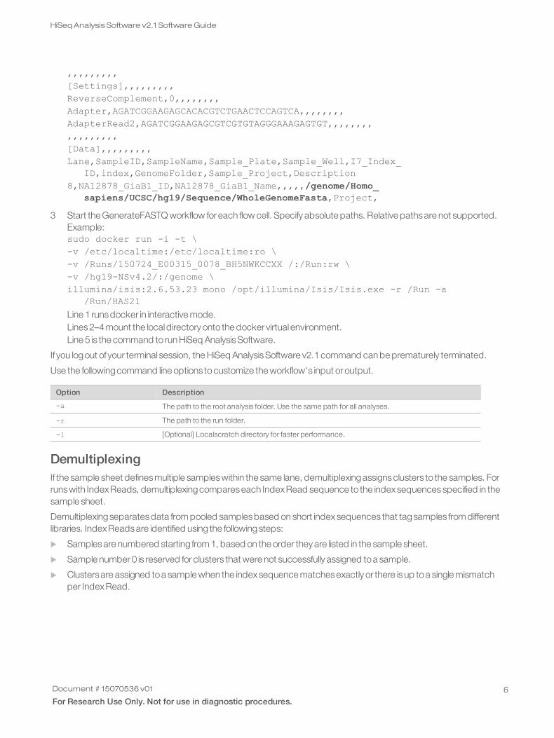
GenerateFASTQ WorkflowThe first items toprocess in the GenerateFASTQ workflow are the run folderswith base call and quality score data in*.bcl.gz file format. The workflow demultiplexes the data and converts it toFASTQ filesorganized under a per-sampledirectory structure.

Initially, you create a SampleSheet.csv file for the GenerateFASTQ workflow step. Anew sample sheet file isautomatically generated for each step, specifying the settings that will be applied in subsequent steps. For moreinformation, see Sample Sheet on page 20.

Run GenerateFASTQ1 Identify a run folder for the analysis, which can be the original run folder for the flow cell.

2 In the top levelof the run folder, create a sample sheet named SampleSheet.csv, asshown in the example below.Make sure that the GenomeFolder location iscorrect.For more information, see Sample Sheet on page 20.

[Header],,,,,,,,,IEMFileVersion,4,,,,,,,,Investigator Name,S. w.,,,,,,,,Experiment Name,,,,,,,,,Date,2/12/2015,,,,,,,,Workflow,GenerateFastq,,,,,,,,Application,HiSeq FASTQ Only,,,,,,,,Assay,TruSeq HT,,,,,,,,Description,HiSeqX run,,,,,,,,Chemistry,Default,,,,,,,,,,,,,,,,,[Reads],,,,,,,,,151,,,,,,,,,151,,,,,,,,,

Document # 15070536 v01



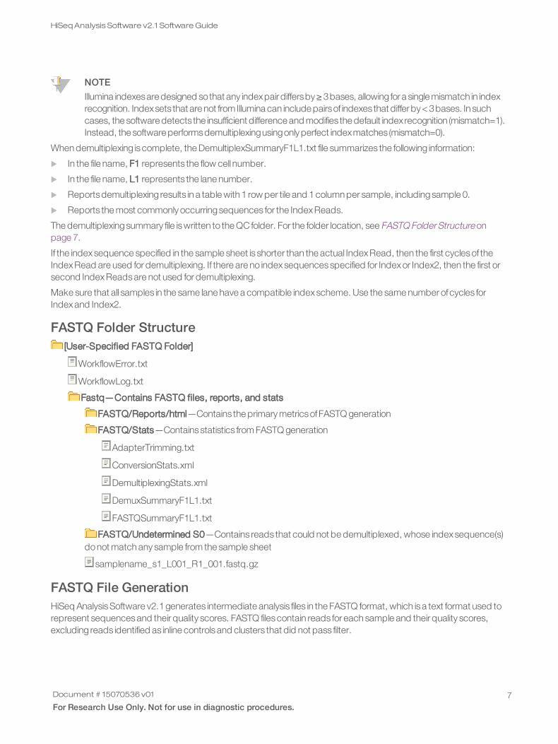
,,,,,,,,,[Settings],,,,,,,,,ReverseComplement,0,,,,,,,,Adapter,AGATCGGAAGAGCACACGTCTGAACTCCAGTCA,,,,,,,,AdapterRead2,AGATCGGAAGAGCGTCGTGTAGGGAAAGAGTGT,,,,,,,,,,,,,,,,,[Data],,,,,,,,,Lane,SampleID,SampleName,Sample_Plate,Sample_Well,I7_Index_

ID,index,GenomeFolder,Sample_Project,Description8,NA12878_GiaB1_ID,NA12878_GiaB1_Name,,,,,/genome/Homo_

sapiens/UCSC/hg19/Sequence/WholeGenomeFasta,Project,

3 Start the GenerateFASTQ workflow for each flow cell. Specify absolute paths. Relative pathsare not supported.Example:sudo docker run -i -t \-v /etc/localtime:/etc/localtime:ro \-v /Runs/150724_E00315_0078_BH5NWKCCXX /:/Run:rw \-v /hg19-NSv4.2/:/genome \illumina/isis:2.6.53.23 mono /opt/illumina/Isis/Isis.exe -r /Run -a

/Run/HAS21

Line 1 runsdocker in interactive mode.Lines2–4mount the localdirectory onto the docker virtual environment.Line 5 is the command to run HiSeq AnalysisSoftware.

If you logout of your terminal session, the HiSeq AnalysisSoftware v2.1command can be prematurely terminated.

Use the followingcommand line options tocustomize the workflow's input or output.

Option Description

-a The path to the root analysis folder. Use the same path for all analyses.

-r The path to the run folder.

-l [Optional] Localscratch directory for faster performance.

DemultiplexingIf the sample sheet definesmultiple sampleswithin the same lane, demultiplexingassignsclusters to the samples. Forrunswith IndexReads, demultiplexingcompareseach IndexRead sequence to the indexsequencesspecified in thesample sheet.

Demultiplexingseparatesdata from pooled samplesbased on short indexsequences that tagsamples from differentlibraries. IndexReadsare identified using the followingsteps:

u Samplesare numbered starting from 1, based on the order they are listed in the sample sheet.

u Sample number 0 is reserved for clusters that were not successfully assigned toa sample.

u Clustersare assigned toa sample when the indexsequence matchesexactly or there isup toa single mismatchper IndexRead.

Document # 15070536 v01



NOTE

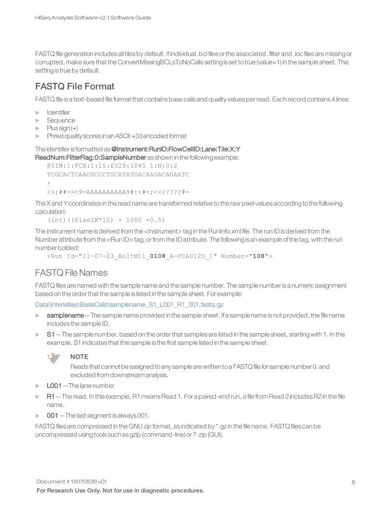
Illumina indexesare designed sothat any indexpairdiffersby≥ 3bases, allowing fora single mismatch in indexrecognition. Indexsets that are not from Illumina can include pairsof indexes that differby< 3bases. In suchcases, the software detects the insufficient difference and modifies the default indexrecognition (mismatch=1).Instead, the software performsdemultiplexingusingonlyperfect indexmatches (mismatch=0).

When demultiplexing iscomplete, the DemultiplexSummaryF1L1.txt file summarizes the following information:

u In the file name, F1 represents the flow cell number.

u In the file name, L1 represents the lane number.

u Reportsdemultiplexing results in a table with 1 row per tile and 1column per sample, includingsample 0.

u Reports the most commonly occurringsequences for the IndexReads.

The demultiplexingsummary file iswritten to the QCfolder. For the folder location, see FASTQ Folder Structure onpage 7.

If the indexsequence specified in the sample sheet is shorter than the actual IndexRead, then the first cyclesof theIndexRead are used for demultiplexing. If there are no indexsequencesspecified for Indexor Index2, then the first orsecond IndexReadsare not used for demultiplexing.

Make sure that all samples in the same lane have a compatible indexscheme. Use the same number ofcycles forIndexand Index2.

FASTQ Folder Structure[User-Specified FASTQ Folder]

WorkflowError.txt

WorkflowLog.txt

Fastq—Contains FASTQ files, reports, and stats

FASTQ/Reports/html—Contains the primary metricsofFASTQ generation

FASTQ/Stats—Containsstatistics from FASTQ generation

AdapterTrimming.txt

ConversionStats.xml

DemultiplexingStats.xml

DemuxSummaryF1L1.txt

FASTQSummaryF1L1.txt

FASTQ/Undetermined S0—Contains reads that could not be demultiplexed, whose indexsequence(s)donot match any sample from the sample sheet

samplename_s1_L001_R1_001.fastq.gz

FASTQ File GenerationHiSeq AnalysisSoftware v2.1generates intermediate analysis files in the FASTQ format, which isa text format used torepresent sequencesand their quality scores. FASTQ filescontain reads for each sample and their quality scores,excluding reads identified as inline controlsand clusters that did not pass filter.

Document # 15070536 v01



FASTQ file generation includesall tilesby default. If individual .bcl filesor the associated .filter and .loc filesare missingorcorrupted, make sure that the ConvertMissingBCLsToNoCalls setting is set to true (value=1) in the sample sheet. Thissetting is true by default.

FASTQ File FormatFASTQ file isa text-based file format that containsbase calls and quality valuesper read. Each record contains4 lines:

u Identifieru Sequenceu Plussign (+)u Phred quality scores inanASCII +33encoded format

The identifier is formatted as@Instrument:RunID:FlowCellID:Lane:Tile:X:YReadNum:FilterFlag:0:SampleNumber asshown in the followingexample:

@SIM:1:FCX:1:15:6329:1045 1:N:0:2TCGCACTCAACGCCCTGCATATGACAAGACAGAATC+<>;##=><9=AAAAAAAAAA9#:<#<;<<<????#=

The X and Y coordinates in the read name are transformed relative to the raw pixel valuesaccording to the followingcalculation:

(int)((PixelX*10) + 1000 +0.5)

The instrument name isderived from the <Instrument> tag in the RunInfo.xml file. The run ID isderived from theNumber attribute from the <Run ID> tag, or from the ID attribute. The following isan example of the tag, with the runnumber bolded:

<Run Id="11-07-23_BoltM11_0108_A-FCA012D_1" Number="108">

FASTQ File NamesFASTQ filesare named with the sample name and the sample number. The sample number isa numeric assignmentbased on the order that the sample is listed in the sample sheet. For example:

Data\Intensities\BaseCalls\samplename_S1_L001_R1_001.fastq.gz

u samplename—The sample name provided in the sample sheet. If a sample name isnot provided, the file nameincludes the sample ID.

u S1—The sample number, based on the order that samplesare listed in the sample sheet, startingwith 1. In thisexample, S1 indicates that this sample is the first sample listed in the sample sheet.

NOTE

Readsthat cannot be assigned toanysample are written toa FASTQ file for sample number0, andexcluded from downstream analysis.

u L001—The lane number.

u R1—The read. In thisexample, R1meansRead 1. For a paired-end run, a file from Read 2 includesR2 in the filename.

u 001—The last segment isalways001.

FASTQ filesare compressed in the GNU zip format, as indicated by *.gz in the file name. FASTQ filescan beuncompressed using tools such asgzip (command-line) or 7-zip (GUI).

Document # 15070536 v01



QC Files and Other Output FilesToperform QC, first use the SequencingAnalysisViewer (SAV) toview important quality metrics. If the generatedFASTQ filesare empty or nearly empty, view the output files for possible errors.

If the run doesnot include indexes, view the following files.

File Description

WorkflowError.txtWorkflowLog.txt

Processing logs that contain additional information on the run.

InterOp files in the InterOp folder Contain the %Q30 scores and additional information for QC.

FastqSummaryF1L*.txt Contains the number of raw and PF clusters for each lane and tile on a per sample basis.

If the run includes indexes, view the following files in addition to the files listed above.

File Description

IndexMetricsOut.bin SAV uses this file with the other files in the InterOp folder.

DemultiplexSummaryF1L1.txt Contains the percentage of each index sample for each lane and tile. This file also liststhe most frequent indexes (unique or combination) found in the lanes. View this file whena sample has too many reads or no reads.

AdapterTrimming.txt Lists the number of trimmed bases and percentage of bases for each tile. This file ispresent only if adapter trimming was specified for the run.

Undetermined_S0_L00*_R*_001.gz Contains the reads with unidentifiable index reads. This file is present only whendemultiplexing.

The following filesare alsooutput from the GenerateFASTQ workflow.

File Description

CompletedJobInfo.xml Written after analysis iscomplete. Contains information about the run, suchasdate, flow cell ID, software version, and other parameters.

ConversionStats.xml Conversion statisticsper tile, includingraw cluster count, read number, yieldQ30, yield, and quality score. Alsoconversion statisticsper lane, including lanenumber.

DemultiplexingStatx.xml Demultiplexingstatisticsper lane, barcode, sample, project, and flow cell.

SampleSheetUsed.csv Sample sheet copied from the run folder

Resequencing Analysis WorkflowThe Resequencinganalysisworkflow uses the Isaac Aligner and Strelka Germline Variant Caller tocompare the DNAsequence in the sample against the human reference genome hg19. It identifiesany small variants (SNPsor indels) andlarge structural variants (SVsand CNVs) relative to the reference sequence.

The Resequencingworkflow uses the run folder as input.

The main output filesare BAM files (containing the readsafter alignment), VCF files (containing the variant calls),Genome VCF files (describing the calls for all variant and nonvariant sites in the genome), and SV VCF files (describingthe calls for structural variantsand copy number variants in the genome).

Document # 15070536 v01



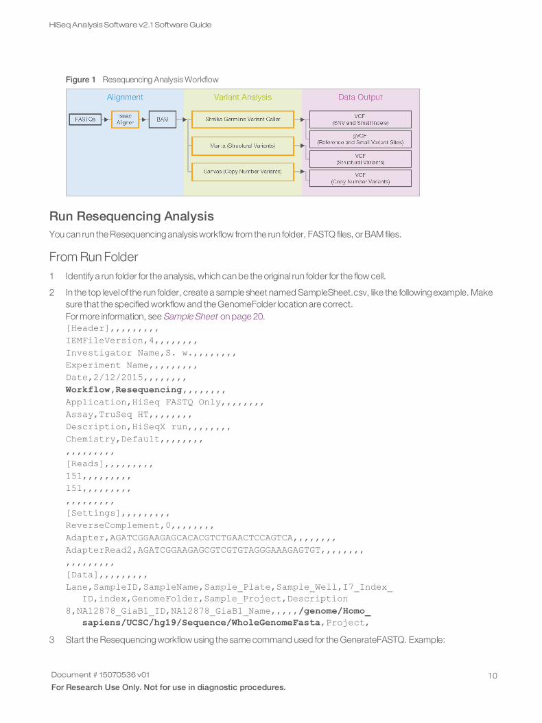
Figure 1 Resequencing Analysis Workflow

Run Resequencing AnalysisYou can run the Resequencinganalysisworkflow from the run folder, FASTQ files, or BAM files.

From Run Folder1 Identify a run folder for the analysis, which can be the original run folder for the flow cell.

2 In the top levelof the run folder, create a sample sheet named SampleSheet.csv, like the followingexample. Makesure that the specified workflow and the GenomeFolder location are correct.For more information, see Sample Sheet on page 20.[Header],,,,,,,,,IEMFileVersion,4,,,,,,,,Investigator Name,S. w.,,,,,,,,Experiment Name,,,,,,,,,Date,2/12/2015,,,,,,,,Workflow,Resequencing,,,,,,,,Application,HiSeq FASTQ Only,,,,,,,,Assay,TruSeq HT,,,,,,,,Description,HiSeqX run,,,,,,,,Chemistry,Default,,,,,,,,,,,,,,,,,[Reads],,,,,,,,,151,,,,,,,,,151,,,,,,,,,,,,,,,,,,[Settings],,,,,,,,,ReverseComplement,0,,,,,,,,Adapter,AGATCGGAAGAGCACACGTCTGAACTCCAGTCA,,,,,,,,AdapterRead2,AGATCGGAAGAGCGTCGTGTAGGGAAAGAGTGT,,,,,,,,,,,,,,,,,[Data],,,,,,,,,Lane,SampleID,SampleName,Sample_Plate,Sample_Well,I7_Index_

ID,index,GenomeFolder,Sample_Project,Description8,NA12878_GiaB1_ID,NA12878_GiaB1_Name,,,,,/genome/Homo_

sapiens/UCSC/hg19/Sequence/WholeGenomeFasta,Project,

3 Start the Resequencingworkflow using the same command used for the GenerateFASTQ. Example:

Document # 15070536 v01



sudo docker run -i -t \-v /etc/localtime:/etc/localtime:ro \-v /Runs/150724_E00315_0078_BH5NWKCCXX /:/Run:rw \-v /hg19-NSv4.2/:/genome \illumina/isis:2.6.53.23 mono /opt/illumina/Isis/Isis.exe -r /Run -a

/Run/HAS21

If available, fast localscratch is recommended. Use the followingexample command if using localscratch.sudo docker run -i -t \-v /etc/localtime:/etc/localtime:ro \–v /mnt/localscratch:/localscratch:rw ]\-v /Runs/150724_E00315_0078_BH5NWKCCXX/:/Run:rw ]\-v /hg19-NSv4.2/:/genome/illumina/isis:2.6.53.23 mono /opt/illumina/Isis/Isis.exe \-r /Run -a /Run/HAS21 –l /localscratch

From FASTQ Files1 Make sure that the FASTQ filesmeet the followingcriteria:

u All FASTQ filesare gzipped and have the file extension *.fastq.gz.u FASTQ filenamescontain the string *_R1.fastq.gz or *_R1_*.fastq.gz for read 1. For paired-end samples, the

matching read 2 filescontain the same stringswith R2 instead ofR1. Lowercase r isalsoacceptable.u Only the last occurrence ofa matching_R1_ or _R2_ in the file name isused. For example:

u sample_r1_R1_fastq.gz and sample_r1_R2_fastq.gz worksand is treated asa paired-end dataset.u sample_r1_R2_fastq.gz and sample_r2_R2_fastq.gz doesnot work and givesan error about a missing

read 1FASTQ file tomatch the read 2FASTQ file.u sample_r1_R1_fastq.gz and sample_r2_R1_fastq.gz works, but is treated as2separate read 1FASTQ

files for a single-end dataset rather than a paired-end dataset.

2 In the top levelof the run folder, create a sample sheet named SampleSheet.csv.u In the Settingssection, add FastqInput,UseExistingu In the Data section, add FastqFolder asanother columnExample:[Header]Workflow,Resequencing[Settings]TranscriptSource,refseqRunSVDetection,1RunCNVDetection,1FastqInput,UseExisting[Data]SampleID,SampleName,GenomeFolder,Lanes,PloidyX,PloidyY,FastqFolderNA12878_micro,NA12878_micro, /genome/Homo_

sapiens/UCSC/hg19/Sequence/WholeGenomeFasta,1,2,0, /Runs/150724_E00315_0078_BH5NWKCCXX/bcl2fastq_out

3 Start the Resequencingworkflow using the same command used for the GenerateFASTQ. Example:sudo docker run -i -t \-v /etc/localtime:/etc/localtime:ro \-v /Runs/150724_E00315_0078_BH5NWKCCXX /:/Run:rw \

Document # 15070536 v01



-v /hg19-NSv4.2/:/genome \illumina/isis:2.6.53.23 mono /opt/illumina/Isis/Isis.exe -r /Run -a

/Run/HAS21

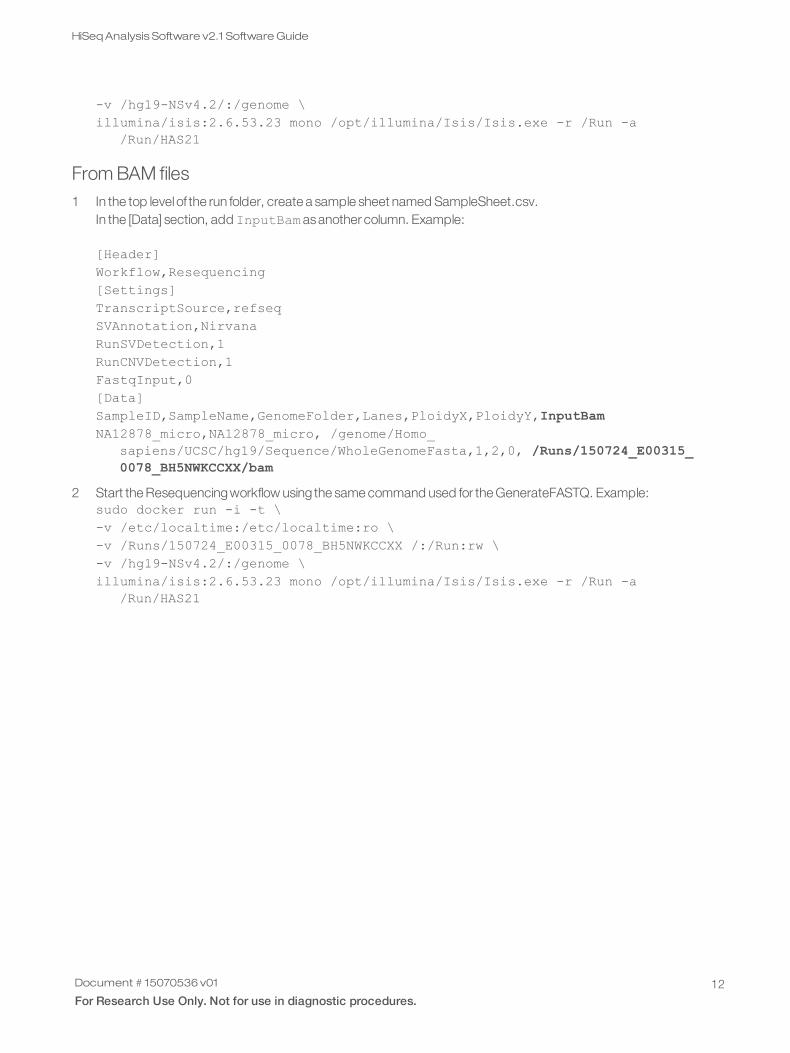
From BAM files1 In the top levelof the run folder, create a sample sheet named SampleSheet.csv.

In the [Data] section, add InputBam asanother column. Example:

[Header]Workflow,Resequencing[Settings]TranscriptSource,refseqSVAnnotation,NirvanaRunSVDetection,1RunCNVDetection,1FastqInput,0[Data]SampleID,SampleName,GenomeFolder,Lanes,PloidyX,PloidyY,InputBamNA12878_micro,NA12878_micro, /genome/Homo_

sapiens/UCSC/hg19/Sequence/WholeGenomeFasta,1,2,0, /Runs/150724_E00315_0078_BH5NWKCCXX/bam

2 Start the Resequencingworkflow using the same command used for the GenerateFASTQ. Example:sudo docker run -i -t \-v /etc/localtime:/etc/localtime:ro \-v /Runs/150724_E00315_0078_BH5NWKCCXX /:/Run:rw \-v /hg19-NSv4.2/:/genome \illumina/isis:2.6.53.23 mono /opt/illumina/Isis/Isis.exe -r /Run -a

/Run/HAS21

Document # 15070536 v01



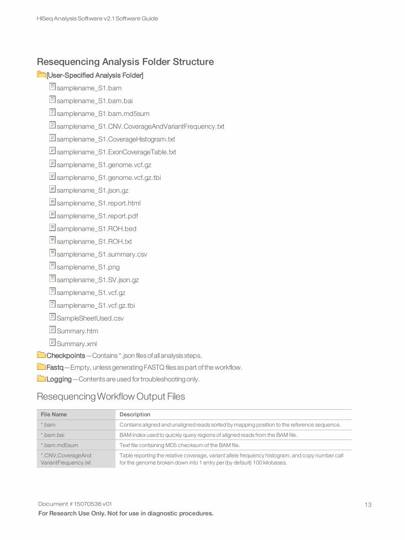
Resequencing Analysis Folder Structure[User-Specified Analysis Folder]

samplename_S1.bam

samplename_S1.bam.bai

samplename_S1.bam.md5sum

samplename_S1.CNV.CoverageAndVariantFrequency.txt

samplename_S1.CoverageHistogram.txt

samplename_S1.ExonCoverageTable.txt

samplename_S1.genome.vcf.gz

samplename_S1.genome.vcf.gz.tbi

samplename_S1.json.gz

samplename_S1.report.html

samplename_S1.report.pdf

samplename_S1.ROH.bed

samplename_S1.ROH.txt

samplename_S1.summary.csv

samplename_S1.png

samplename_S1.SV.json.gz

samplename_S1.vcf.gz

samplename_S1.vcf.gz.tbi

SampleSheetUsed.csv

Summary.htm

Summary.xml

Checkpoints—Contains *.json filesofall analysis steps.

Fastq—Empty, unlessgeneratingFASTQ filesaspart of the workflow.

Logging—Contentsare used for troubleshootingonly.

Resequencing Workflow Output Files

File Name Description

*.bam Contains aligned and unaligned reads sorted by mapping position to the reference sequence.

*.bam.bai BAM index used to quickly query regions of aligned reads from the BAM file.

*.bam.md5sum Text file containing MD5 checksum of the BAM file.

*.CNV.CoverageAndVariantFrequency.txt

Table reporting the relative coverage, variant allele frequency histogram, and copy number callfor the genome broken down into 1 entry per (by default) 100 kilobases.

Document # 15070536 v01



File Name Description

*.CoverageHistogram.txt Contains coverage depth information for every chromosome. This file can be used to generate acoverage histogram.

*.ExonCoverageTable.txt Tab-delimited file providingchromosome, start, stop, name, median coverage,and percent call ability for all exons.

*.genome.vcf.gz gVCF file containing variant and small variant calls. A tabix index file is also produced.

*.json.gz Extended annotation data for the SNVs and indels.

*.report.pdf / *.report.html Summary report for the sample. Provides several high-level statistics pulled from *.summary.csv,such as genome coverage and % aligned.

*.ROH.bed A .bed file of the ROH calls. Contains extra colums (4) ROH score, (5) number of unfilteredhomozygous alternate calls in the ROH, and (6) number of unfiltered heterozygous SNV calls inthe ROH.

*.ROH.txt A text file reporting overall metrics of the ROH caller. Reported metrics are percent SNVs in ROH,unfiltered het/hom, filtered het/hom (large ROH), percent SNVs in large ROH, and number oflarge ROH.

*.summary.csv Summary statistics for the sample, for parsing by downstream tools.

*.summary.png A genome-wide view of b-allele frequencies, and structural variants.

*.SV.vcf.gz VCF file containing SV and CNV calls. Also includes reference calls from the CNV caller. A *.jsonand a tabix index file also gets produced.

*.vcf.gz VCF file containing variant calls. A tabix index file is also produced.

SampleSheetUsed.csv Sample Sheet used for the analysis.

Summary.htm HTML file containing statistics on the flow cell on a per tile basis.

Summary.xml XML version of the summary file.

Resequencing Analysis ReportThe Resequencingworkflow outputsa PDF and an HTML report that providesan overview ofstatisticsper sample.

Sample InformationThe Sample Information table providesstatisticsabout the sample and alignment quality.

Statistic Definition

Total PF Reads The total number of reads passing filter.

% Q30 Bases The percentage of bases with a quality score of 30 or higher.

Total Aligned Reads 1 and 2 The total number of aligned reads for reads 1 and 2.

% Aligned Reads 1 and 2 The percentage of aligned passing filter reads for reads 1 and 2.

Total Aligned Bases Reads 1and 2

The total number of aligned bases for reads 1 and 2.

% Aligned Bases Reads 1and 2

The percentage of aligned bases for reads 1 and 2.

Mismatch Rate Reads 1 and2

The average percentage of mismatches of reads 1 and 2 over all cycles.

Coverage HistogramThe Coverage histogram shows the number of reference basesplotted against the depth ofcoverage.

Document # 15070536 v01



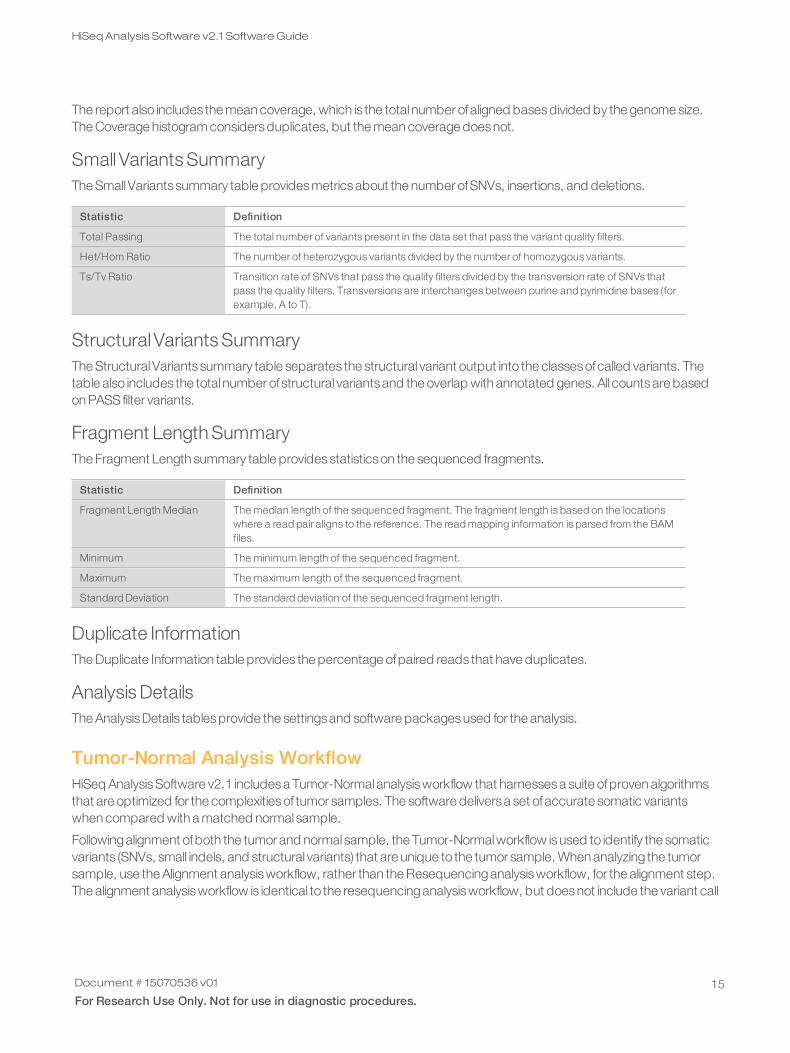
The report also includes the mean coverage, which is the total number ofaligned basesdivided by the genome size.The Coverage histogram considersduplicates, but the mean coverage doesnot.

Small Variants SummaryThe SmallVariantssummary table providesmetricsabout the number ofSNVs, insertions, and deletions.


Total Passing The total number of variants present in the data set that pass the variant quality filters.

Het/Hom Ratio The number of heterozygous variants divided by the number of homozygous variants.

Ts/Tv Ratio Transition rate of SNVs that pass the quality filters divided by the transversion rate of SNVs thatpass the quality filters. Transversions are interchanges between purine and pyrimidine bases (forexample, A to T).

StructuralVariants SummaryThe StructuralVariantssummary table separates the structural variant output into the classesofcalled variants. Thetable also includes the total number of structural variantsand the overlap with annotated genes. All countsare basedon PASS filter variants.

Fragment Length SummaryThe Fragment Length summary table providesstatisticson the sequenced fragments.


Fragment Length Median The median length of the sequenced fragment. The fragment length is based on the locationswhere a read pair aligns to the reference. The read mapping information is parsed from the BAMfiles.

Minimum The minimum length of the sequenced fragment.

Maximum The maximum length of the sequenced fragment.

Standard Deviation The standard deviation of the sequenced fragment length.

Duplicate InformationThe Duplicate Information table provides the percentage ofpaired reads that have duplicates.

Analysis DetailsThe AnalysisDetails tablesprovide the settingsand software packagesused for the analysis.

Tumor-Normal Analysis WorkflowHiSeq AnalysisSoftware v2.1 includesa Tumor-Normalanalysisworkflow that harnessesa suite ofproven algorithmsthat are optimized for the complexitiesof tumor samples. The software deliversa set ofaccurate somatic variantswhen compared with a matched normal sample.

Followingalignment ofboth the tumor and normal sample, the Tumor-Normalworkflow isused to identify the somaticvariants (SNVs, small indels, and structural variants) that are unique to the tumor sample. When analyzing the tumorsample, use the Alignment analysisworkflow, rather than the Resequencinganalysisworkflow, for the alignment step.The alignment analysisworkflow is identical to the resequencinganalysisworkflow, but doesnot include the variant call

Document # 15070536 v01



analysis. The variant call analysisused in the Resequencinganalysisworkflow isnot valid for a tumor sample, whichcan contain somatic variants. The variant callingmethodsused in the Resequencinganalysisworkflow assume adiploid genotype.

For optimal results, Illumina recommendsa minimum coverage of30x for the normal sample and 60xcoverage for thetumor sample.

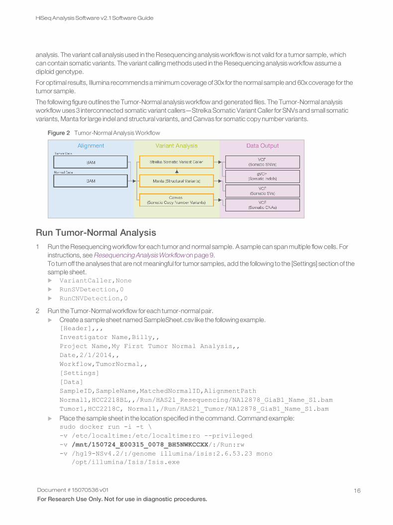
The following figure outlines the Tumor-Normalanalysisworkflow and generated files. The Tumor-Normalanalysisworkflow uses3 interconnected somatic variant callers—Strelka Somatic Variant Caller for SNVsand small somaticvariants, Manta for large indel and structural variants, and Canvas for somatic copy number variants.

Figure 2 Tumor-Normal Analysis Workflow

Run Tumor-Normal Analysis1 Run the Resequencingworkflow for each tumor and normal sample. Asample can span multiple flow cells. For

instructions, see ResequencingAnalysisWorkflow on page 9.To turn off the analyses that are not meaningful for tumor samples, add the following to the [Settings] section of thesample sheet.u VariantCaller,Noneu RunSVDetection,0u RunCNVDetection,0

2 Run the Tumor-Normalworkflow for each tumor-normalpair.u Create a sample sheet named SampleSheet.csv like the followingexample.

[Header],,,Investigator Name,Billy,,Project Name,My First Tumor Normal Analysis,,Date,2/1/2014,,Workflow,TumorNormal,,[Settings][Data]SampleID,SampleName,MatchedNormalID,AlignmentPathNormal1,HCC2218BL,,/Run/HAS21_Resequencing/NA12878_GiaB1_Name_S1.bamTumor1,HCC2218C, Normal1,/Run/HAS21_Tumor/NA12878_GiaB1_Name_S1.bam

u Place the sample sheet in the location specified in the command. Command example:sudo docker run -i -t \-v /etc/localtime:/etc/localtime:ro --privileged-v /mnt/150724_E00315_0078_BH5NWKCCXX/:/Run:rw-v /hg19-NSv4.2/:/genome illumina/isis:2.6.53.23 mono

/opt/illumina/Isis/Isis.exe

Document # 15070536 v01



-r /Run/HAS21_TumorNormalSampleSheet-a /Run/HAS21_TumorNormal

The command assumes that the sample sheet isplaced in /mnt/150724_E00315_0078_BH5NWKCCXX/HAS21_TumorNormalSampleSheet.The command alsospecifies that the location for the analysisoutput is /mnt/150724_E00315_0078_BH5NWKCCXX/HAS21_TumorNormal.

Use the followingcommand line options tocustomize the run.

Option Description

-l [Optional] The path to the local storage. If specified, the input files for the specifiedworkflow are copied to the local storage of the compute node (local hard drive).If there is available storage on the local node, the -loption is recommended asstandard practice.

Tumor-Normal Analysis Folder Structure[User-Specified Analysis Folder]

Checkpoint.txt

CompletedJobInfo.xml

normalsample_tumorsample_G1_P1.somatic.json.gz

normalsamplename_tumorsamplename _G1_P1.somatic.json.gz

normalsamplename_tumorsamplename _G1_P1.somatic.SV.vcf.gz

normalsamplename_tumorsamplename _G1_P1.somatic.SV.vcf.gz.bi

normalsamplename_tumorsamplename _G1_P1.somatic.vcf.gz

normalsamplename_tumorsamplename _G1_P1.somatic.vcf.gz.tbi

ploidy.bed.gz

ploidy.bed.gz.tbi

SampleSheetUsed.csv

WorkflowError.txt

WorkflowLog.txt

LoggingTemp—Used for troubleshootingonly.

CNV_G1_P1—Used for troubleshootingonly.

Tumor-NormalWorkflow Output Files

File Description

*.somatic.vcf.gz VCF containing somatic SNVs and small indels identified by Strelka. A tabix index file is alsoproduced.

*.somatic.json.gz Extended annotation data for the somatic SNVs and indels.

*.somatic.SV.vcf.tz VCF containing somatic SVs and CNVs identified by Manta and Canvas, respectively. EstimatedPloidy and purity are included in the VCF header. A tabix index file is also produced.

*.summary.png A genome-wide view of coverage levels, b-allele frequencies, and structural variants.

Document # 15070536 v01



File Description

*.report.pdf A high-level sample report including important metrics, plot of the coverage histogram, settingsused, and tool versions.

*.summary.csv List of all available metrics for the normal and tumor samples. For more information, seeSummary Metrics on page 18.

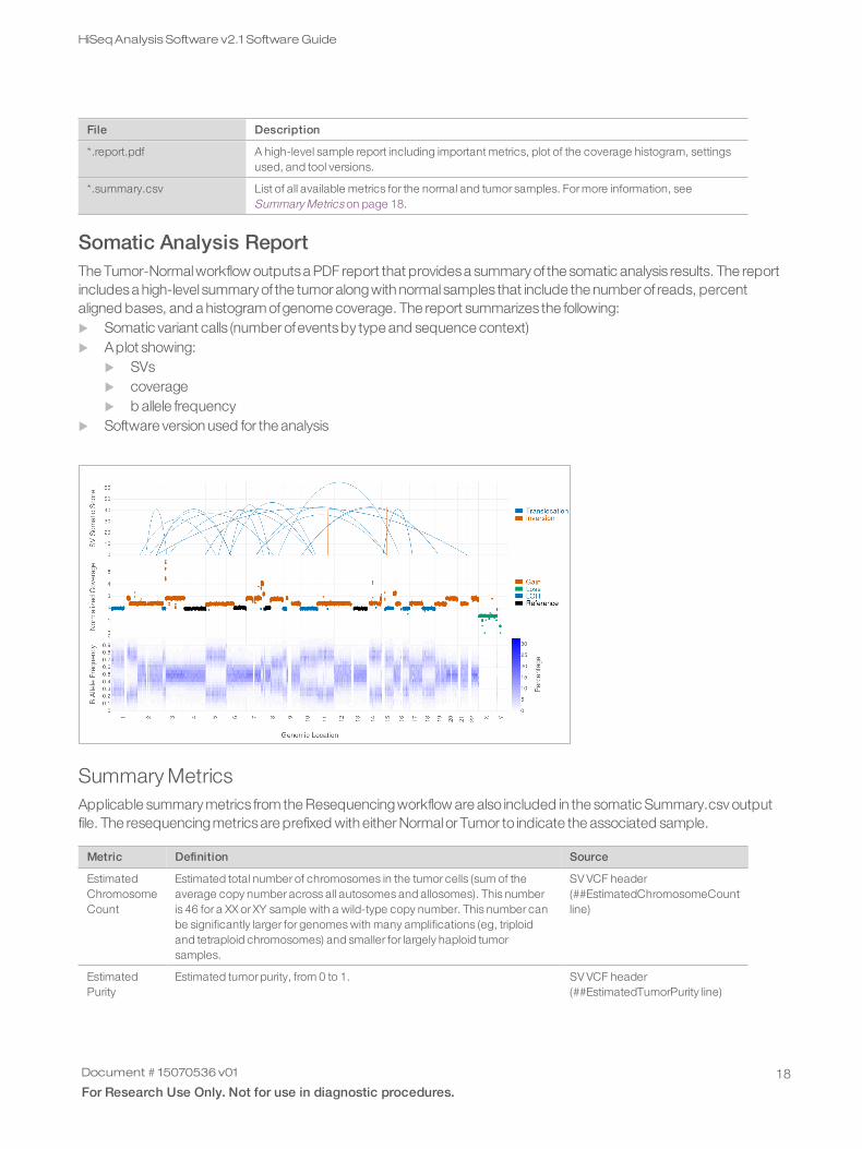
Somatic Analysis ReportThe Tumor-Normalworkflow outputsa PDF report that providesa summary of the somatic analysis results. The reportincludesa high-level summary of the tumor alongwith normal samples that include the number of reads, percentaligned bases, and a histogram ofgenome coverage. The report summarizes the following:u Somatic variant calls (number ofeventsby type and sequence context)u Aplot showing:

u SVsu coverageu b allele frequency

u Software version used for the analysis

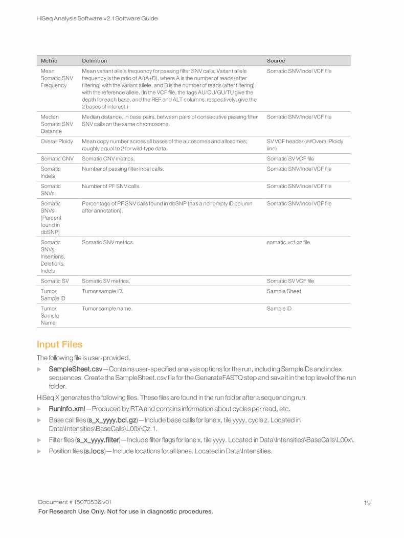
Summary MetricsApplicable summary metrics from the Resequencingworkflow are also included in the somatic Summary.csv outputfile. The resequencingmetricsare prefixed with either Normalor Tumor to indicate the associated sample.

Metric Definition Source

EstimatedChromosomeCount

Estimated total number of chromosomes in the tumor cells (sum of theaverage copy number across all autosomes and allosomes). This numberis 46 for a XX or XY sample with a wild-type copy number. This number canbe significantly larger for genomes with many amplifications (eg, triploidand tetraploid chromosomes) and smaller for largely haploid tumorsamples.

SV VCF header(##EstimatedChromosomeCountline)

EstimatedPurity

Estimated tumor purity, from 0 to 1. SV VCF header(##EstimatedTumorPurity line)

Document # 15070536 v01



Metric Definition Source

MeanSomatic SNVFrequency

Mean variant allele frequency for passing filter SNV calls. Variant allelefrequency is the ratio of A/(A+B), where A is the number of reads (afterfiltering) with the variant allele, and B is the number of reads (after filtering)with the reference allele. (In the VCF file, the tags AU/CU/GU/TU give thedepth for each base, and the REF and ALT columns, respectively, give the2 bases of interest.)

Somatic SNV/Indel VCF file

MedianSomatic SNVDistance

Median distance, in base pairs, between pairs of consecutive passing filterSNV calls on the same chromosome.


Overall Ploidy Mean copy number across all bases of the autosomes and allosomes;roughly equal to 2 for wild-type data.

SV VCF header (##OverallPloidyline)

Somatic CNV Somatic CNV metrics. Somatic SV VCF file

SomaticIndels

Number of passing filter indel calls. Somatic SNV/Indel VCF file

SomaticSNVs

Number of PF SNV calls. Somatic SNV/Indel VCF file

SomaticSNVs(Percentfound indbSNP)

Percentage of PF SNV calls found in dbSNP (has a nonempty ID columnafter annotation).


SomaticSNVs,Insertions,Deletions,Indels

Somatic SNV metrics. somatic.vcf.gz file

Somatic SV Somatic SV metrics. Somatic SV VCF file

TumorSample ID

Tumor sample ID. Sample Sheet

TumorSampleName

Tumor sample name. Sample ID

Input FilesThe following file isuser-provided.

u SampleSheet.csv—Containsuser-specified analysisoptions for the run, includingSampleIDsand indexsequences. Create the SampleSheet.csv file for the GenerateFASTQ step and save it in the top levelof the runfolder.

HiSeq X generates the following files. These filesare found in the run folder after a sequencing run.

u RunInfo.xml—Produced by RTAand contains information about cyclesper read, etc.

u Base call files (s_x_yyyy.bcl.gz)—Include base calls for lane x, tile yyyy, cycle z. Located inData\Intensities\BaseCalls\L00x\Cz.1.

u Filter files (s_x_yyyy.filter)—Include filter flags for lane x, tile yyyy. Located in Data\Intensities\BaseCalls\L00x\.

u Position files (s.locs)—Include locations for all lanes. Located in Data\Intensities.

Document # 15070536 v01



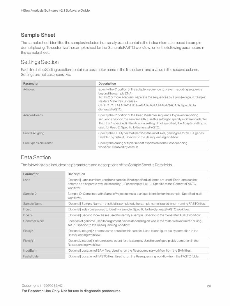
Sample SheetThe sample sheet identifies the samples included in an analysisand contains the index information used in sampledemultiplexing. Tocustomize the sample sheet for the GenerateFASTQ workflow, enter the followingparameters inthe sample sheet.

Settings SectionEach line in the Settingssection containsa parameter name in the first column and a value in the second column.Settingsare not case-sensitive.

Parameter Description

Adapter Specify the 5' portion of the adapter sequence to prevent reporting sequencebeyond the sample DNA.To trim 2 or more adapters, separate the sequences by a plus (+) sign. (Example:Nextera Mate Pair Libraries –CTGTCTCTTATACACATCT+AGATGTGTATAAGAGACAG). Specific toGenerateFASTQ.

AdapterRead2 Specify the 5' portion of the Read 2 adapter sequence to prevent reportingsequence beyond the sample DNA. Use this setting to specify a different adapterthan the 1 specified in the Adapter setting. If not specified, the Adapter setting isused for Read 2. Specific to GenerateFASTQ.

RunHLATyping Specify the HLA typer that identifies the most likely genotypes for 6 HLA genes.Disabled by default. Specific to the Resequencing workflow.

RunExpansionHunter Specify the calling of triplet repeat expansion in the Resequencingworkflow. Disabled by default.

Data SectionThe following table includes the parametersand descriptionsof the Sample Sheet'sData fields.

Parameter Description

Lane [Optional] Lane numbers used for a sample. If not specified, all lanes are used. Each lane can beentered as a separate row, delimited by +. For example: 1+2+3. Specific to the GenerateFASTQworkflow.

SampleID Sample ID. Combined with SampleProject to make a unique identifier for the sample. Specified in allworkflows.

SampleName [Optional] Sample Name. If this field is completed, the sample name is used when naming FASTQ files.

Index [Optional] Index bases used to identify a sample. Specific to the GenerateFASTQ workflow.

Index2 [Optional] Second index bases used to identify a sample. Specific to the GenerateFASTQ workflow.

GenomeFolder Location of genome used for alignment. Varies depending on where the folder was extracted duringsetup. Specific to the Resequencing workflow.

PloidyX [Optional, integer] X chromosome count for this sample. Used to configure ploidy correction in theResequencing workflow.

PloidyY [Optional, integer] Y chromosome count for this sample. Used to configure ploidy correction in theResequencing workflow.

InputBam [Optional] Location of BAM files. Used to run the Resequencing workflow from the BAM files.

FastqFolder [Optional] Location of FASTQ files. Used to run the Resequencing workflow from the FASTQ folder.

Document # 15070536 v01



Methods for the Resequencing WorkflowThissection describes the methodologies for the Resequencingand Alignment algorithm in HiSeq AnalysisSoftwarev2.1. The Resequencinganalysisand Alignment analysisworkflowsare identical, except that the Alignment analysisworkflow doesnot contain variant callingand isonly recommended for tumor samples.

OverviewAfter the sequencer generatesbase calls and quality scores, the resultingdata get aligned to the reference genome.Next, assembly and variant callingoccurs.

Alignment and variant callinghappen within Isaac Aligner, Starling, Canvas, and Manta, producing the followingoutput:

u Realigned and duplicate marked reads in a BAM file format.

u Variants in a VCF file format.

u An additionalGenome VCF (gVCF) file. This file featuresan entry for every base in the reference, whichdifferentiates reference calls and nocalls, and a summary ofquality. The reference calls are block compressedand all single nucleotide polymorphismsand indelsare included. StructuralVariantsand CNVsare contained inseparate files.

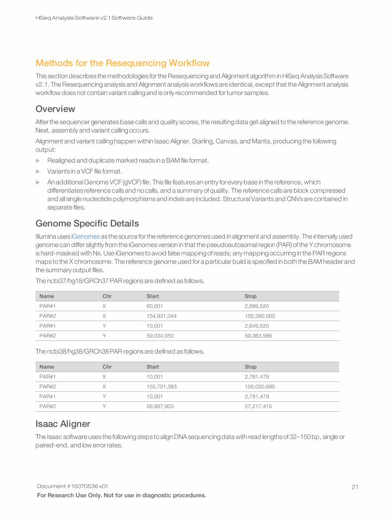
Genome Specific DetailsIllumina uses iGenomesas the source for the reference genomesused in alignment and assembly. The internally usedgenome can differ slightly from the iGenomesversion in that the pseudoautosomal region (PAR) of the Y chromosomeishard-masked with Ns. Use iGenomes toavoid false mappingof reads; any mappingoccurring in the PAR regionsmaps to the X chromosome. The reference genome used for a particular build is specified in both the BAM header andthe summary output files.

The ncbi37/hg18/GRCh37PAR regionsare defined as follows.

Name Chr Start Stop

PAR#1 X 60,001 2,699,520

PAR#2 X 154,931,044 155,260,560

PAR#1 Y 10,001 2,649,520

PAR#2 Y 59,034,050 59,363,566

The ncbi38/hg38/GRCh38PAR regionsare defined as follows.

Name Chr Start Stop

PAR#1 X 10,001 2,781,479

PAR#2 X 155,701,383 156,030,895

PAR#1 Y 10,001 2,781,479

PAR#2 Y 56,887,903 57,217,415

Isaac AlignerThe Isaac software uses the followingsteps toalign DNAsequencingdata with read lengthsof32–150bp, single orpaired-end, and low error rates.

Document # 15070536 v01



https://support.illumina.com/sequencing/sequencing_software/igenome.html

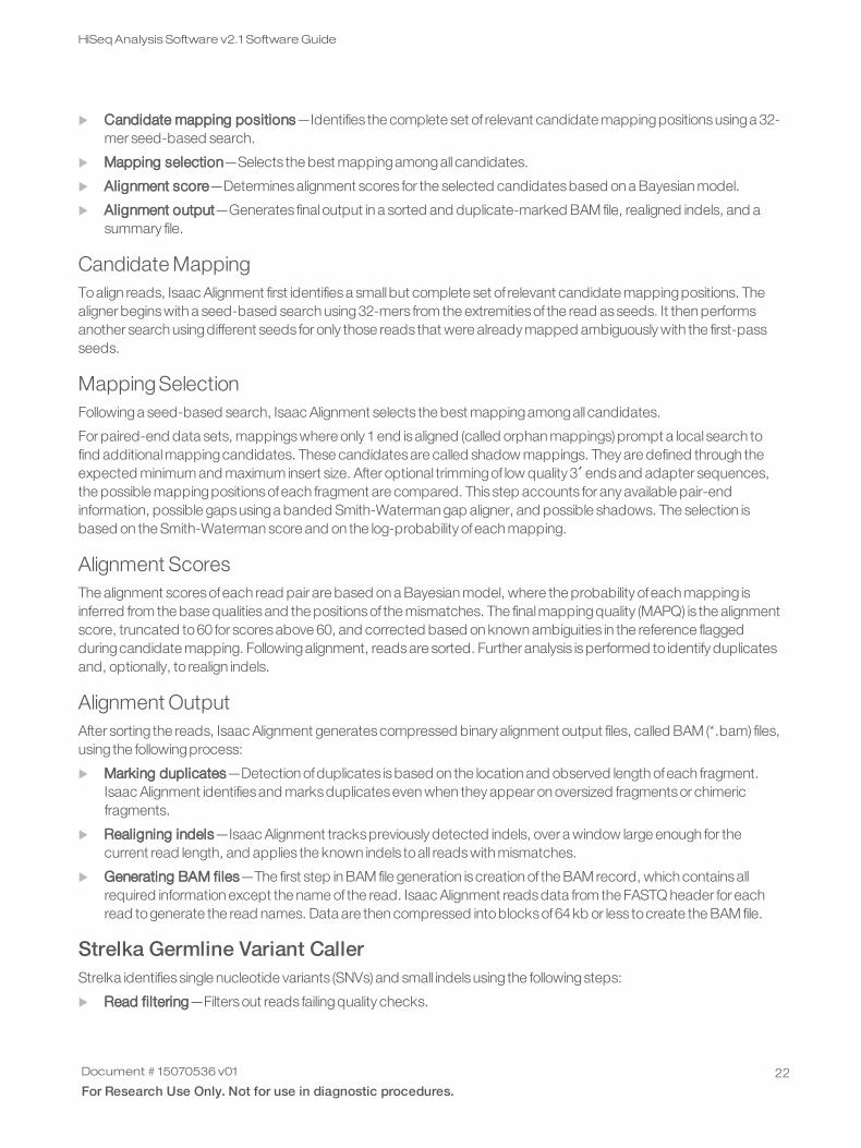
u Candidate mapping positions—Identifies the complete set of relevant candidate mappingpositionsusinga 32-mer seed-based search.

u Mapping selection—Selects the best mappingamongall candidates.

u Alignment score—Determinesalignment scores for the selected candidatesbased on a Bayesian model.

u Alignment output—Generates finaloutput in a sorted and duplicate-marked BAM file, realigned indels, and asummary file.

Candidate MappingToalign reads, Isaac Alignment first identifiesa small but complete set of relevant candidate mappingpositions. Thealigner beginswith a seed-based search using32-mers from the extremitiesof the read asseeds. It then performsanother search usingdifferent seeds for only those reads that were already mapped ambiguously with the first-passseeds.

Mapping SelectionFollowinga seed-based search, Isaac Alignment selects the best mappingamongall candidates.

For paired-end data sets, mappingswhere only 1end isaligned (called orphan mappings) prompt a local search tofind additionalmappingcandidates. These candidatesare called shadow mappings. They are defined through theexpected minimum and maximum insert size. After optional trimmingof low quality 3′endsand adapter sequences,the possible mappingpositionsofeach fragment are compared. This step accounts for any available pair-endinformation, possible gapsusinga banded Smith-Waterman gap aligner, and possible shadows. The selection isbased on the Smith-Waterman score and on the log-probability ofeach mapping.

Alignment ScoresThe alignment scoresofeach read pair are based on a Bayesian model, where the probability ofeach mapping isinferred from the base qualitiesand the positionsof the mismatches. The finalmappingquality (MAPQ) is the alignmentscore, truncated to60 for scoresabove 60, and corrected based on known ambiguities in the reference flaggedduringcandidate mapping. Followingalignment, readsare sorted. Further analysis isperformed to identify duplicatesand, optionally, to realign indels.

Alignment OutputAfter sorting the reads, Isaac Alignment generatescompressed binary alignment output files, called BAM (*.bam) files,using the followingprocess:

u Marking duplicates—Detection ofduplicates isbased on the location and observed length ofeach fragment.Isaac Alignment identifiesand marksduplicateseven when they appear on oversized fragmentsor chimericfragments.

u Realigning indels—Isaac Alignment trackspreviously detected indels, over a window large enough for thecurrent read length, and applies the known indels toall readswith mismatches.

u Generating BAM files—The first step in BAM file generation iscreation of the BAM record, which containsallrequired information except the name of the read. Isaac Alignment readsdata from the FASTQ header for eachread togenerate the read names. Data are then compressed intoblocksof64kb or less tocreate the BAM file.

Strelka Germline Variant CallerStrelka identifiessingle nucleotide variants (SNVs) and small indelsusing the followingsteps:

u Read filtering—Filtersout reads failingquality checks.

Document # 15070536 v01



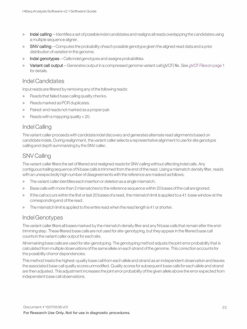
u Indel calling—Identifiesa set ofpossible indel candidatesand realignsall readsoverlapping the candidatesusinga multiple sequence aligner.

u SNV calling—Computes the probability ofeach possible genotype given the aligned read data and a priordistribution of variation in the genome.

u Indel genotypes—Calls indelgenotypesand assignsprobabilities.

u Variant call output—Generatesoutput in a compressed genome variant call (gVCF) file. See gVCF Fileson page 1for details.

IndelCandidatesInput readsare filtered by removingany of the following reads:

u Reads that failed base callingquality checks.

u Readsmarked asPCR duplicates.

u Paired-end readsnot marked asa proper pair.

u Readswith a mappingquality < 20.

IndelCallingThe variant caller proceedswith candidate indeldiscovery and generatesalternate read alignmentsbased oncandidate indels. During realignment, the variant caller selectsa representative alignment touse for site genotypecallingand depth summarizingby the SNV caller.

SNV CallingThe variant caller filters the set of filtered and realigned reads for SNV callingwithout affecting indel calls. Anycontiguous trailingsequence ofNbase calls is trimmed from the end of the read. Usinga mismatch density filter, readswith an unexpectedly high number ofdisagreementswith the reference are masked as follows.

u The variant caller identifieseach insertion or deletion asa single mismatch.

u Base callswith more than 2mismatches to the reference sequence within 20basesof the call are ignored.

u If the call occurswithin the first or last 20basesofa read, the mismatch limit is applied toa 41-base window at thecorrespondingend of the read.

u The mismatch limit is applied to the entire read when the read length is41or shorter.

IndelGenotypesThe variant caller filtersall basesmarked by the mismatch density filter and any Nbase calls that remain after the end-trimmingstep. These filtered base calls are not used for site-genotyping, but they appear in the filtered base callcounts in the variant caller output for each site.

All remainingbase calls are used for site-genotyping. The genotypingmethod adjusts the joint error probability that iscalculated from multiple observationsof the same allele on each strand of the genome. Thiscorrection accounts forthe possibility oferror dependencies.

Thismethod treats the highest-quality base call from each allele and strand asan independent observation and leavesthe associated base call quality scoresunmodified. Quality scores for subsequent base calls for each allele and strandare then adjusted. Thisadjustment increases the joint error probability of the given allele above the error expected fromindependent base call observations.

Document # 15070536 v01



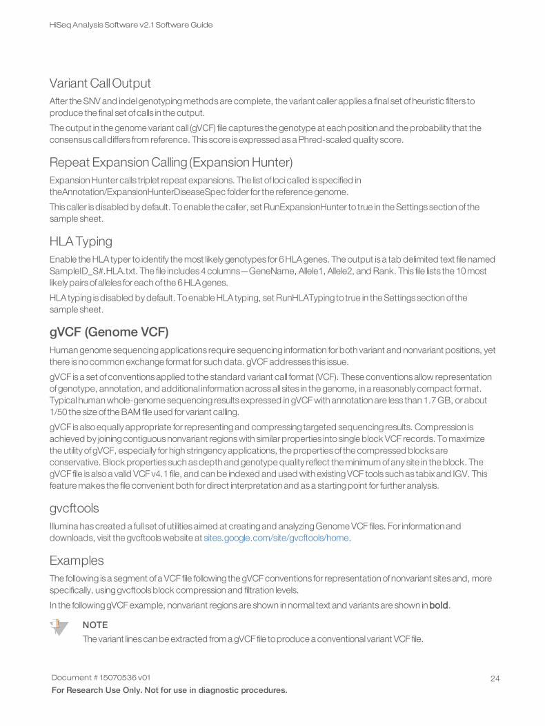
Variant CallOutputAfter the SNV and indelgenotypingmethodsare complete, the variant caller appliesa final set ofheuristic filters toproduce the final set ofcalls in the output.

The output in the genome variant call (gVCF) file captures the genotype at each position and the probability that theconsensuscall differs from reference. This score isexpressed asa Phred-scaled quality score.

Repeat Expansion Calling (Expansion Hunter)Expansion Hunter calls triplet repeat expansions. The list of loci called is specified intheAnnotation/ExpansionHunterDiseaseSpec folder for the reference genome.

Thiscaller isdisabled by default. Toenable the caller, set RunExpansionHunter to true in the Settingssection of thesample sheet.

HLA TypingEnable the HLA typer to identify the most likely genotypes for 6HLAgenes. The output isa tab delimited text file namedSampleID_S#.HLA.txt. The file includes4columns—GeneName, Allele1, Allele2, and Rank. This file lists the 10mostlikely pairsofalleles for each of the 6HLAgenes.

HLA typing isdisabled by default. Toenable HLA typing, set RunHLATyping to true in the Settingssection of thesample sheet.

gVCF (Genome VCF)Human genome sequencingapplications require sequencing information for both variant and nonvariant positions, yetthere isnocommon exchange format for such data. gVCF addresses this issue.

gVCF isa set ofconventionsapplied to the standard variant call format (VCF). These conventionsallow representationofgenotype, annotation, and additional information acrossall sites in the genome, in a reasonably compact format.Typical human whole-genome sequencing resultsexpressed in gVCF with annotation are less than 1.7GB, or about1/50 the size of the BAM file used for variant calling.

gVCF isalsoequally appropriate for representingand compressing targeted sequencing results. Compression isachieved by joiningcontiguousnonvariant regionswith similar properties intosingle block VCF records. Tomaximizethe utility ofgVCF, especially for high stringency applications, the propertiesof the compressed blocksareconservative. Block propertiessuch asdepth and genotype quality reflect the minimum ofany site in the block. ThegVCF file isalsoa valid VCF v4.1 file, and can be indexed and used with existingVCF toolssuch as tabixand IGV. Thisfeature makes the file convenient both for direct interpretation and asa startingpoint for further analysis.

gvcftoolsIllumina hascreated a full set ofutilitiesaimed at creatingand analyzingGenome VCF files. For information anddownloads, visit the gvcftoolswebsite at sites.google.com/site/gvcftools/home.

ExamplesThe following isa segment ofa VCF file following the gVCF conventions for representation ofnonvariant sitesand, morespecifically, usinggvcftoolsblock compression and filtration levels.

In the followinggVCF example, nonvariant regionsare shown in normal text and variantsare shown in bold.

NOTE

The variant linescanbe extracted from a gVCF file toproduce a conventionalvariant VCF file.

Document # 15070536 v01



https://sites.google.com/site/gvcftools/home

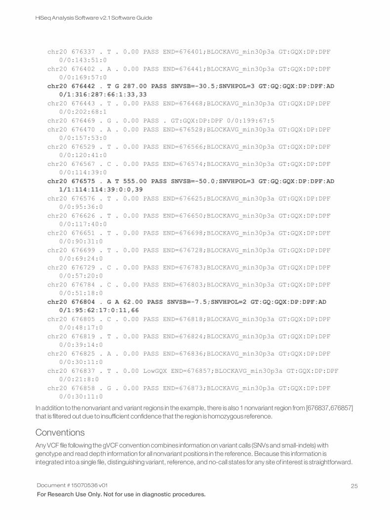
chr20 676337 . T . 0.00 PASS END=676401;BLOCKAVG_min30p3a GT:GQX:DP:DPF0/0:143:51:0

chr20 676402 . A . 0.00 PASS END=676441;BLOCKAVG_min30p3a GT:GQX:DP:DPF0/0:169:57:0

chr20 676442 . T G 287.00 PASS SNVSB=-30.5;SNVHPOL=3 GT:GQ:GQX:DP:DPF:AD0/1:316:287:66:1:33,33

chr20 676443 . T . 0.00 PASS END=676468;BLOCKAVG_min30p3a GT:GQX:DP:DPF0/0:202:68:1

chr20 676469 . G . 0.00 PASS . GT:GQX:DP:DPF 0/0:199:67:5chr20 676470 . A . 0.00 PASS END=676528;BLOCKAVG_min30p3a GT:GQX:DP:DPF

0/0:157:53:0chr20 676529 . T . 0.00 PASS END=676566;BLOCKAVG_min30p3a GT:GQX:DP:DPF

0/0:120:41:0chr20 676567 . C . 0.00 PASS END=676574;BLOCKAVG_min30p3a GT:GQX:DP:DPF

0/0:114:39:0chr20 676575 . A T 555.00 PASS SNVSB=-50.0;SNVHPOL=3 GT:GQ:GQX:DP:DPF:AD

1/1:114:114:39:0:0,39chr20 676576 . T . 0.00 PASS END=676625;BLOCKAVG_min30p3a GT:GQX:DP:DPF






0/0:51:18:0chr20 676804 . G A 62.00 PASS SNVSB=-7.5;SNVHPOL=2 GT:GQ:GQX:DP:DPF:AD

0/1:95:62:17:0:11,66chr20 676805 . C . 0.00 PASS END=676818;BLOCKAVG_min30p3a GT:GQX:DP:DPF


0/0:39:14:0chr20 676825 . A . 0.00 PASS END=676836;BLOCKAVG_min30p3a GT:GQX:DP:DPF

0/0:30:11:0chr20 676837 . T . 0.00 LowGQX END=676857;BLOCKAVG_min30p3a GT:GQX:DP:DPF

0/0:21:8:0chr20 676858 . G . 0.00 PASS END=676873;BLOCKAVG_min30p3a GT:GQX:DP:DPF

0/0:30:11:0

In addition to the nonvariant and variant regions in the example, there isalso1nonvariant region from [676837,676857]that is filtered out due to insufficient confidence that the region ishomozygous reference.

ConventionsAny VCF file following the gVCF convention combines information on variant calls (SNVsand small-indels) withgenotype and read depth information for all nonvariant positions in the reference. Because this information isintegrated intoa single file, distinguishingvariant, reference, and no-call states for any site of interest is straightforward.

Document # 15070536 v01



The followingsubsectionsdescribe the general conventions followed in any gVCF file, and provide information on thespecific parametersand filtersused in the Isaac workflow gVCF output.

NOTE

gVCFconventionsare writtenwith the assumption that onlyone sample per file isbeingrepresented.

InterpretationgVCFs file can be interpreted as follows:

u Fast interpretation—Asa discrete classification of the genome intovariant, reference, and no-call loci. Thisclassification is the simplest way touse the gVCF. The Filter fields for the gVCF file have already been set tomarkuncertain calls as filtered for both variant and nonvariant positions. Simple analysiscan be performed to look for alllociwith a filter value ofPASSand treat them ascalled.

u Research interpretation—Asa statisticalgenome. Additional fields, such asgenotype quality, are provided forboth variant and reference positions toallow the threshold between called and uncalled sites tobe varied. Thesefieldscan alsobe used toapply more stringent criteria toa set of loci from an initial screen.

External ToolsgVCF iswritten to the VCF 4.1specifications, soany tool that iscompatible with the specification (such as IGV andtabix) can use the file. However, certain toolsare not appropriate if they:

u Apply algorithms toVCF files that make sense for only variant calls (asopposed tovariant and nonvariant regions inthe full gVCF)

u Are only computationally feasible for variant calls

For these cases, extract the variant calls from the full gVCF file.

Special Handling for Indel ConflictsSites that are filled in inside deletionshave additional treatment.

u Heterozygous Deletions—Sites inside heterozygousdeletionshave haploid genotype entries (ie, 0 instead of0/0, 1 instead of1/1). HeterozygousSNVsare marked with the SiteConflict filter and their originalgenotype is leftunchanged. Sites inside heterozygousdeletionscannot have a genotype quality score higher than the enclosingdeletion genotype quality.

u Homozygous Deletions—Sites inside homozygousdeletionshave genotype set toperiod (.), and site andgenotype quality are alsoset toperiod (.).

u All Deletions—Sites inside any deletion are marked with the filtersof the deletion, and more filterscan be addedpertaining to the site itself. These modifications reflect the idea that the enclosing indel confidence bounds the siteconfidence.

u Indel Conflicts—In any region where overlappingdeletion evidence cannot be resolved into2haplotypes, allindel and set records in the region are marked with the IndelConflict filter.

ID Type Description

IndelConflict site/indel Locus is in region with conflicting indel calls.

SiteConflict site Site genotype conflicts with proximal indel call. This conflict is typically a heterozygous genotype foundinside a heterozygous deletion.

Table 1 Indel Conflict Filters

Document # 15070536 v01



Representation of Nonvariant SegmentsThissection includes the followingsubsections:

u Block representation usingEND key

u Joiningnonvariant sites intoa single block record

u Block sample values

u Nonvariant block implementations

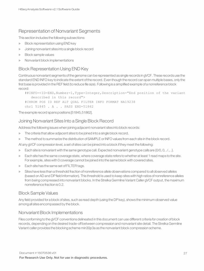
Block Representation Using END KeyContinuousnonvariant segmentsof the genome can be represented assingle records in gVCF. These recordsuse thestandard END INFO key to indicate the extent of the record. Even though the record can span multiple bases, only thefirst base isprovided in the REF field (to reduce file size). Following isa simplified example ofa nonreference blockrecord:

##INFO=<ID=END,Number=1,Type=Integer,Description="End position of the variantdescribed in this record">

#CHROM POS ID REF ALT QUAL FILTER INFO FORMAT NA19238chr1 51845 . A . . PASS END=51862

The example record spanspositions [51845,51862].

Joining Nonvariant Sites Into a Single Block RecordAddress the following issueswhen joiningadjacent nonvariant sites intoblock records:

u The criteria that allow adjacent sites tobe joined intoa single block record.

u The method tosummarize the distribution ofSAMPLE or INFO values from each site in the block record.

At any gVCF compression level, a set of sitescan be joined intoa block if they meet the following:

u Each site isnonvariant with the same genotype call. Expected nonvariant genotype calls are {0/0, 0, ./., .}.

u Each site has the same coverage state, where coverage state refers towhether at least 1 read maps to the site.For example, siteswith 0coverage cannot be joined into the same block with covered sites.

u Each site has the same set ofFILTER tags.

u Siteshave less than a threshold fraction ofnonreference allele observationscompared toall observed alleles(based on AD and DP field information). This threshold isused tokeep siteswith high ratiosofnonreference allelesfrom beingcompressed intononvariant blocks. In the Strelka Germline Variant Caller gVCF output, the maximumnonreference fraction is0.2.

Block Sample ValuesAny field provided for a block of sites, such as read depth (using the DPkey), shows the minimum observed valueamongall sitesencompassed by the block.

Nonvariant Block ImplementationsFilesconforming to the gVCF conventionsdelineated in thisdocument can use different criteria for creation ofblockrecords, dependingon the desired trade-offbetween compression and nonvariant site detail. The Strelka GermlineVariant caller provides the blockingscheme min30p3a as the nonvariant block compression scheme.

Document # 15070536 v01



Each sample value shown for the block, such as the depth (using the DPkey), is restricted tohave a range where themaximum value iswithin 30% or 3of the minimum. Therefore, for sample value range [x,y], y ≤ x+max(3, x*0.3). Thisrange restriction applies toall sample valueswritten in the finalblock record.

Genotype Quality for Variant and Nonvariant SitesThe gVCF file usesan adapted version ofgenotype quality for variant and nonvariant site filtration. This value isassociated with the GQX key. The GQX value is intended to represent the minimum ofPhred genotype quality(assuming the site is variant, assuming the sites isnonvariant).

You can use this value toallow a single value tobe used as the primary quality filter for both variant and nonvariant sites.Filteringon this value corresponds toa conservative assumption appropriate for applicationswhere referencegenotype callsmust be determined at the same stringency asvariant genotypes, for example:

u An assertion that a site ishomozygous reference at GQX ≥ 20 ismade assuming the site is variant.

u An assertion that a site isa nonreference genotype at GQX ≥ 20 ismade assuming the site isnonvariant.

Filter CriteriaThe gVCF FILTER description isdivided into2sections, the first describes filteringbased on genotype quality while thesecond describesall other filters.

NOTE

These filtersare default valuesused in the current Strelka Germline Variant Caller implementation. However, noset of filtersorcutoff valuesare required fora file toconform togVCFconventions.

The genotype quality is the primary filter for all sites in the genome. In particular, traditionaldiscovery-based site qualityvalues that convey confidence that the site isanythingbesides the homozygous reference genotype, such asSNV orquality, are not used. Instead, a site, or locus, is filtered based on the confidence in the reported genotype for thecurrent sample.

The genotype quality used in gVCF isa Phred-scaled probability that the given genotype iscorrect. It is indicated withthe FORMAT field tagGQX. Any locuswhere the genotype quality isbelow the cutoff threshold is filtered with the tagLowGQX. Besides filteringon genotype quality, other filterscan alsobe applied.

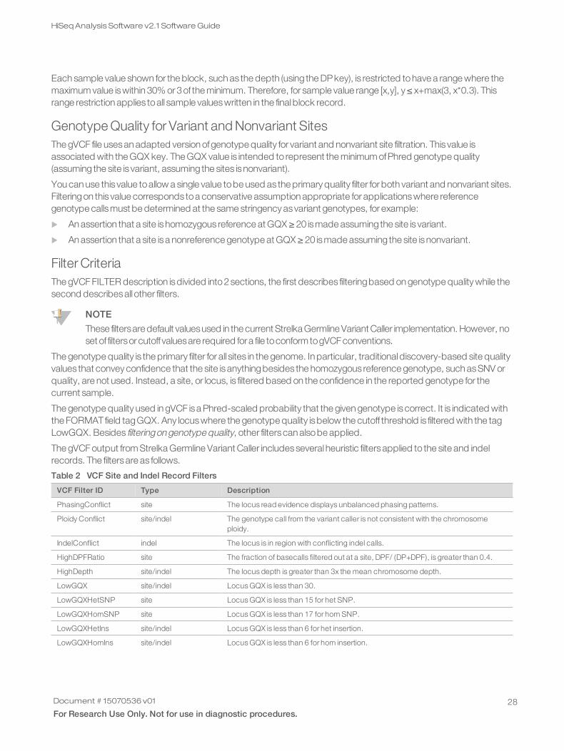
The gVCF output from Strelka Germline Variant Caller includesseveral heuristic filtersapplied to the site and indelrecords. The filtersare as follows.

VCF Filter ID Type Description

PhasingConflict site The locus read evidence displays unbalanced phasing patterns.

Ploidy Conflict site/indel The genotype call from the variant caller is not consistent with the chromosomeploidy.

IndelConflict indel The locus is in region with conflicting indel calls.

HighDPFRatio site The fraction of basecalls filtered out at a site, DPF/ (DP+DPF), is greater than 0.4.

HighDepth site/indel The locus depth is greater than 3x the mean chromosome depth.

LowGQX site/indel Locus GQX is less than 30.

LowGQXHetSNP site Locus GQX is less than 15 for het SNP.

LowGQXHomSNP site Locus GQX is less than 17 for hom SNP.

LowGQXHetIns site/indel Locus GQX is less than 6 for het insertion.

LowGQXHomIns site/indel Locus GQX is less than 6 for hom insertion.

Table 2 VCF Site and Indel Record Filters

Document # 15070536 v01



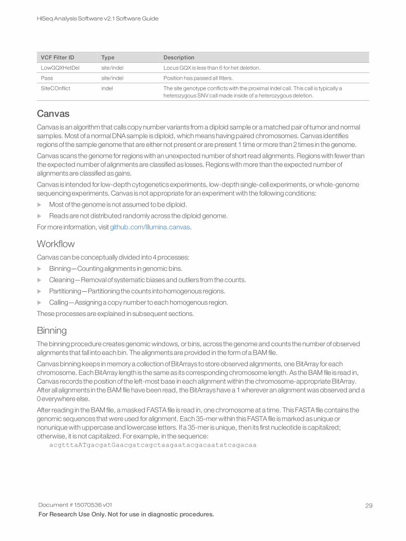
VCF Filter ID Type Description

LowGQXHetDel site/indel Locus GQX is less than 6 for het deletion.

Pass site/indel Position has passed all filters.

SiteCOnflict indel The site genotype conflicts with the proximal indel call. This call is typically aheterozygous SNV call made inside of a heterozygous deletion.

CanvasCanvas isan algorithm that calls copy number variants from a diploid sample or a matched pair of tumor and normalsamples. Most ofa normalDNAsample isdiploid, which meanshavingpaired chromosomes. Canvas identifiesregionsof the sample genome that are either not present or are present 1 time or more than 2 times in the genome.

Canvasscans the genome for regionswith an unexpected number of short read alignments. Regionswith fewer thanthe expected number ofalignmentsare classified as losses. Regionswith more than the expected number ofalignmentsare classified asgains.

Canvas is intended for low-depth cytogeneticsexperiments, low-depth single-cell experiments, or whole-genomesequencingexperiments. Canvas isnot appropriate for an experiment with the followingconditions:

u Most of the genome isnot assumed tobe diploid.

u Readsare not distributed randomly across the diploid genome.

For more information, visit github.com/Illumina.canvas.

WorkflowCanvascan be conceptually divided into4processes:

u Binning—Countingalignments in genomic bins.

u Cleaning—Removalof systematic biasesand outliers from the counts.

u Partitioning—Partitioning the counts intohomogenous regions.

u Calling—Assigninga copy number toeach homogenous region.

These processesare explained in subsequent sections.

BinningThe binningprocedure createsgenomic windows, or bins, across the genome and counts the number ofobservedalignments that fall intoeach bin. The alignmentsare provided in the form ofa BAM file.

Canvasbinningkeeps in memory a collection ofBitArrays tostore observed alignments, one BitArray for eachchromosome. Each BitArray length is the same as itscorrespondingchromosome length. As the BAM file is read in,Canvas records the position of the left-most base in each alignment within the chromosome-appropriate BitArray.After all alignments in the BAM file have been read, the BitArrayshave a 1wherever an alignment wasobserved and a0everywhere else.

After reading in the BAM file, a masked FASTA file is read in, one chromosome at a time. ThisFASTA file contains thegenomic sequences that were used for alignment. Each 35-mer within thisFASTA file ismarked asunique ornonunique with uppercase and lowercase letters. If a 35-mer isunique, then its first nucleotide iscapitalized;otherwise, it isnot capitalized. For example, in the sequence:

acgtttaATgacgatGaacgatcagctaagaatacgacaatatcagacaa

Document # 15070536 v01



http://github.com/Illumina/canvas

The 35-mersmarked asunique are as follows:ATGACGATGAACGATCAGCTAAGAATACGACAATATGACGATGAACGATCAGCTAAGAATACGACAATATGAACGATCAGCTAAGAATACGACAATATCAGACAA

Canvasstores the genomic locationsofunique 35-mers in another collection ofBitArraysanalogous toBitArraysusedtostore alignment positions. Unique positionsand nonunique positionsare marked with 1sand 0s, respectively. Thismarking isused asa mask toguarantee that only alignments that start at unique 35-mer positions in the genome areused.

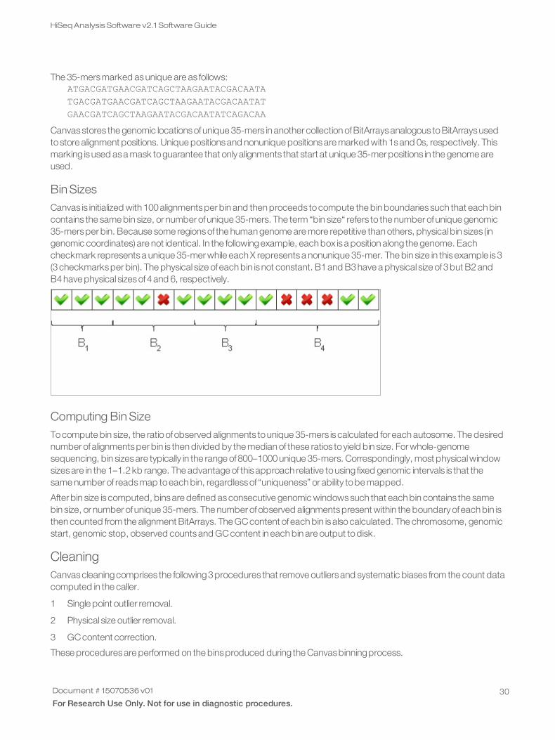
Bin SizesCanvas is initialized with 100alignmentsper bin and then proceeds tocompute the bin boundariessuch that each bincontains the same bin size, or number ofunique 35-mers. The term “bin size“ refers to the number ofunique genomic35-mersper bin. Because some regionsof the human genome are more repetitive than others, physicalbin sizes (ingenomic coordinates) are not identical. In the followingexample, each box isa position along the genome. Eachcheckmark representsa unique 35-mer while each X representsa nonunique 35-mer. The bin size in thisexample is3(3checkmarksper bin). The physical size ofeach bin isnot constant. B1and B3have a physical size of3but B2andB4have physical sizesof4and 6, respectively.

Computing Bin SizeTocompute bin size, the ratioofobserved alignments tounique 35-mers iscalculated for each autosome. The desirednumber ofalignmentsper bin is then divided by the median of these ratios toyield bin size. For whole-genomesequencing, bin sizesare typically in the range of800–1000unique 35-mers. Correspondingly, most physicalwindowsizesare in the 1–1.2kb range. The advantage of thisapproach relative tousing fixed genomic intervals is that thesame number of readsmap toeach bin, regardlessof “uniqueness” or ability tobe mapped.

After bin size iscomputed, binsare defined asconsecutive genomic windowssuch that each bin contains the samebin size, or number ofunique 35-mers. The number ofobserved alignmentspresent within the boundary ofeach bin isthen counted from the alignment BitArrays. The GCcontent ofeach bin isalsocalculated. The chromosome, genomicstart, genomic stop, observed countsand GCcontent in each bin are output todisk.

CleaningCanvascleaningcomprises the following3procedures that remove outliersand systematic biases from the count datacomputed in the caller.

1 Single point outlier removal.

2 Physical size outlier removal.

3 GCcontent correction.

These proceduresare performed on the binsproduced during the Canvasbinningprocess.

Document # 15070536 v01



Single Point Outlier RemovalThisstep removes individualbins that represent extreme outliers. These binshave counts that are very different fromthe countspresent in upstream and downstream bins. Twovalues, a and b, are defined as tobe very different whentheir difference isgreater than expected by chance, assuminga and b come from the same underlyingdistribution.These valuesuse the Chi-squared distribution, as follows:

u µ = 0.5a + 0.5b

u χ2= ((a - µ)2 + (b - µ)2) µ-1

Avalue ofχ2greater than 6.635, which is the 99th percentile of the Chi-squared distribution with 1degree of freedom,isconsidered very different. If a bin count is very different from the count ofboth upstream and downstream neighbors,then the bin isdeemed an outlier and removed.

Physical Size Outlier RemovalBins likely donot have the same physical (genomic) size. The average for whole-genome sequencing runsmight beapproximately 1kb. If the binscover repetitive regionsof the genome, some binssizesmight be severalmegabases insize. Example regionsmight include centromeresand telomeres. The counts in these regions tend tobe unreliable sobinswith extreme physical size are removed. Specifically, the 98th percentile ofobserved physical sizes iscalculatedand binswith sizes larger than this threshold are removed.

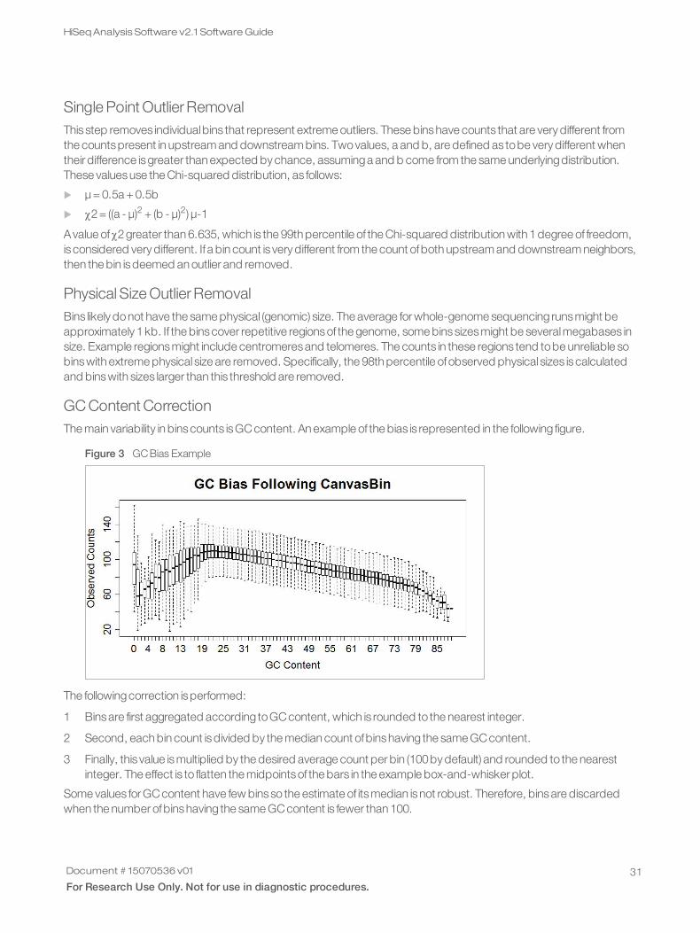
GC Content CorrectionThe main variability in binscounts isGCcontent. An example of the bias is represented in the following figure.

Figure 3 GC Bias Example

The followingcorrection isperformed:

1 Binsare first aggregated according toGCcontent, which is rounded to the nearest integer.

2 Second, each bin count isdivided by the median count ofbinshaving the same GCcontent.

3 Finally, this value ismultiplied by the desired average count per bin (100by default) and rounded to the nearestinteger. The effect is to flatten the midpointsof the bars in the example box-and-whisker plot.

Some values for GCcontent have few binsso the estimate of itsmedian isnot robust. Therefore, binsare discardedwhen the number ofbinshaving the same GCcontent is fewer than 100.

Document # 15070536 v01



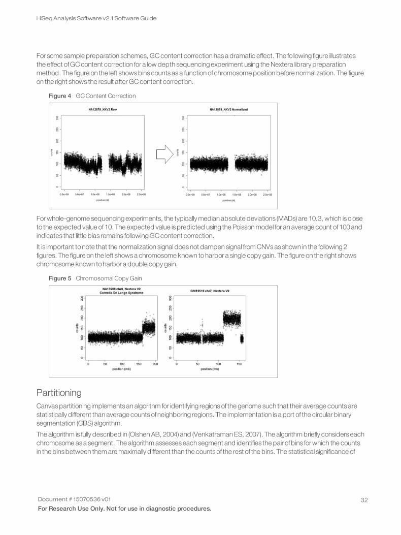
For some sample preparation schemes, GCcontent correction hasa dramatic effect. The following figure illustratesthe effect ofGCcontent correction for a low depth sequencingexperiment using the Nextera library preparationmethod. The figure on the left showsbinscountsasa function ofchromosome position before normalization. The figureon the right shows the result after GCcontent correction.

Figure 4 GC Content Correction

For whole-genome sequencingexperiments, the typically median absolute deviations (MADs) are 10.3, which iscloseto the expected value of10. The expected value ispredicted using the Poisson model for an average count of100andindicates that little bias remains followingGCcontent correction.

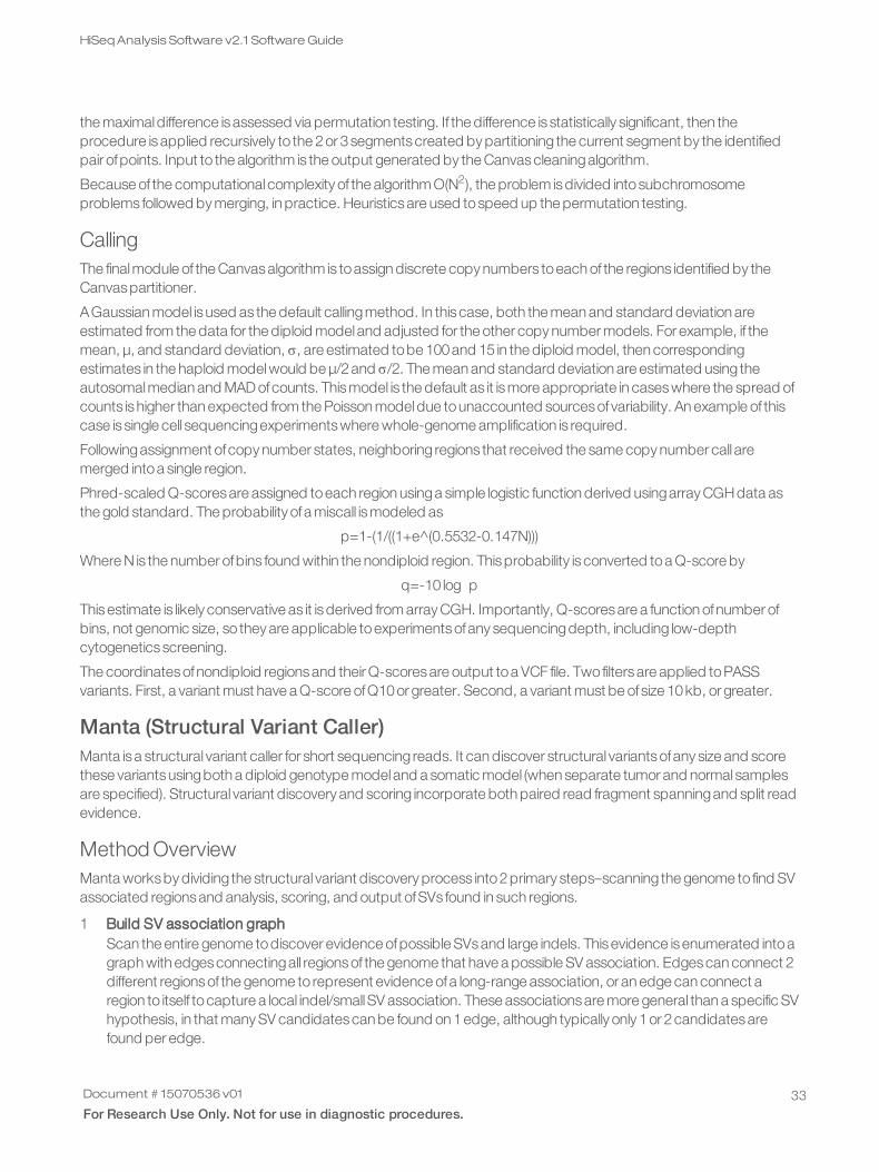
It is important tonote that the normalization signaldoesnot dampen signal from CNVsasshown in the following2figures. The figure on the left showsa chromosome known toharbor a single copy gain. The figure on the right showschromosome known toharbor a double copy gain.

Figure 5 Chromosomal Copy Gain

PartitioningCanvaspartitioning implementsan algorithm for identifying regionsof the genome such that their average countsarestatistically different than average countsofneighboring regions. The implementation isa port of the circular binarysegmentation (CBS) algorithm.

The algorithm is fully described in (Olshen AB, 2004) and (Venkatraman ES, 2007). The algorithm briefly considerseachchromosome asa segment. The algorithm assesseseach segment and identifies the pair ofbins for which the countsin the binsbetween them are maximally different than the countsof the rest of the bins. The statistical significance of

Document # 15070536 v01



the maximaldifference isassessed via permutation testing. If the difference isstatistically significant, then theprocedure isapplied recursively to the 2or 3segmentscreated by partitioning the current segment by the identifiedpair ofpoints. Input to the algorithm is the output generated by the Canvascleaningalgorithm.

Because of the computational complexity of the algorithm O(N2), the problem isdivided intosubchromosomeproblems followed by merging, in practice. Heuristicsare used tospeed up the permutation testing.

CallingThe finalmodule of the Canvasalgorithm is toassign discrete copy numbers toeach of the regions identified by theCanvaspartitioner.

AGaussian model isused as the default callingmethod. In thiscase, both the mean and standard deviation areestimated from the data for the diploid modeland adjusted for the other copy number models. For example, if themean, µ, and standard deviation, σ, are estimated tobe 100and 15 in the diploid model, then correspondingestimates in the haploid modelwould be µ/2and σ/2. The mean and standard deviation are estimated using theautosomalmedian and MAD ofcounts. Thismodel is the default as it ismore appropriate in caseswhere the spread ofcounts ishigher than expected from the Poisson modeldue tounaccounted sourcesof variability. An example of thiscase is single cell sequencingexperimentswhere whole-genome amplification is required.

Followingassignment ofcopy number states, neighboring regions that received the same copy number call aremerged intoa single region.

Phred-scaled Q-scoresare assigned toeach region usinga simple logistic function derived usingarray CGHdata asthe gold standard. The probability ofa miscall ismodeled as

p=1-(1/((1+e^(0.5532-0.147N)))

Where N is the number ofbins found within the nondiploid region. Thisprobability isconverted toa Q-score by

q=-10 log p

Thisestimate is likely conservative as it isderived from array CGH. Importantly, Q-scoresare a function ofnumber ofbins, not genomic size, so they are applicable toexperimentsofany sequencingdepth, including low-depthcytogeneticsscreening.

The coordinatesofnondiploid regionsand their Q-scoresare output toa VCF file. Two filtersare applied toPASSvariants. First, a variant must have a Q-score ofQ10or greater. Second, a variant must be ofsize 10kb, or greater.

Manta (Structural Variant Caller)Manta isa structural variant caller for short sequencing reads. It can discover structural variantsofany size and scorethese variantsusingboth a diploid genotype modeland a somatic model (when separate tumor and normal samplesare specified). Structural variant discovery and scoring incorporate both paired read fragment spanningand split readevidence.

Method OverviewManta worksby dividing the structural variant discovery process into2primary steps–scanning the genome to find SVassociated regionsand analysis, scoring, and output ofSVs found in such regions.

1 Build SV association graphScan the entire genome todiscover evidence ofpossible SVsand large indels. Thisevidence isenumerated intoagraph with edgesconnectingall regionsof the genome that have a possible SV association. Edgescan connect 2different regionsof the genome to represent evidence ofa long-range association, or an edge can connect aregion to itself tocapture a local indel/smallSV association. These associationsare more general than a specific SVhypothesis, in that many SV candidatescan be found on 1edge, although typically only 1or 2candidatesarefound per edge.

Document # 15070536 v01



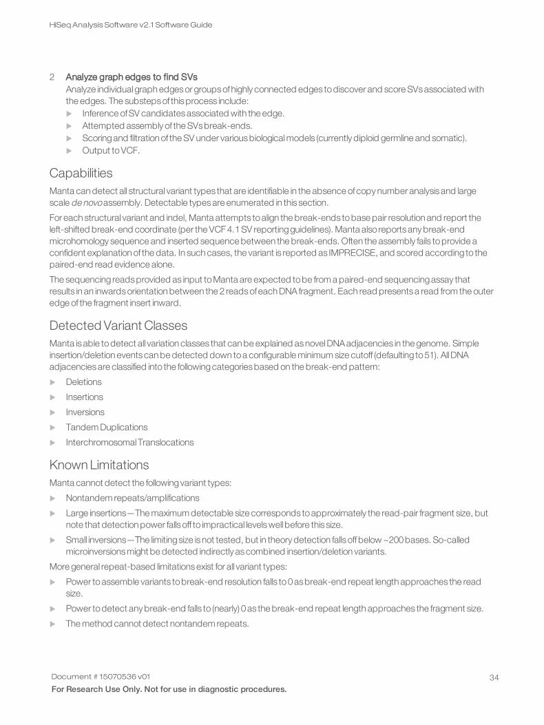
2 Analyze graph edges to find SVsAnalyze individualgraph edgesor groupsofhighly connected edges todiscover and score SVsassociated withthe edges. The substepsof thisprocess include:u Inference ofSV candidatesassociated with the edge.u Attempted assembly of the SVsbreak-ends.u Scoringand filtration of the SV under variousbiologicalmodels (currently diploid germline and somatic).u Output toVCF.

CapabilitiesManta can detect all structural variant types that are identifiable in the absence ofcopy number analysisand largescale de novoassembly. Detectable typesare enumerated in this section.

For each structural variant and indel, Manta attempts toalign the break-ends tobase pair resolution and report theleft-shifted break-end coordinate (per the VCF 4.1SV reportingguidelines). Manta also reportsany break-endmicrohomology sequence and inserted sequence between the break-ends. Often the assembly fails toprovide aconfident explanation of the data. In such cases, the variant is reported as IMPRECISE, and scored according to thepaired-end read evidence alone.

The sequencing readsprovided as input toManta are expected tobe from a paired-end sequencingassay thatresults in an inwardsorientation between the 2 readsofeach DNA fragment. Each read presentsa read from the outeredge of the fragment insert inward.

Detected Variant ClassesManta isable todetect all variation classes that can be explained asnovelDNAadjacencies in the genome. Simpleinsertion/deletion eventscan be detected down toa configurable minimum size cutoff (defaulting to51). AllDNAadjacenciesare classified into the followingcategoriesbased on the break-end pattern:

u Deletions

u Insertions

u Inversions

u Tandem Duplications

u InterchromosomalTranslocations

Known LimitationsManta cannot detect the followingvariant types:

u Nontandem repeats/amplifications

u Large insertions—The maximum detectable size corresponds toapproximately the read-pair fragment size, butnote that detection power fallsoff to impractical levelswell before this size.

u Small inversions—The limitingsize isnot tested, but in theory detection fallsoffbelow ~200bases. So-calledmicroinversionsmight be detected indirectly ascombined insertion/deletion variants.

More general repeat-based limitationsexist for all variant types:

u Power toassemble variants tobreak-end resolution falls to0asbreak-end repeat length approaches the readsize.

u Power todetect any break-end falls to (nearly) 0as the break-end repeat length approaches the fragment size.

u The method cannot detect nontandem repeats.

Document # 15070536 v01



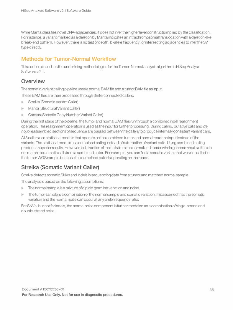
While Manta classifiesnovelDNA-adjacencies, it doesnot infer the higher level constructs implied by the classification.For instance, a variant marked asa deletion by Manta indicatesan intrachromosomal translocation with a deletion-likebreak-end pattern. However, there isno test ofdepth, b-allele frequency, or intersectingadjacencies to infer the SVtype directly.

Methods for Tumor-Normal WorkflowThissection describes the underliningmethodologies for the Tumor-Normalanalysisalgorithm in HiSeq AnalysisSoftware v2.1.

OverviewThe somatic variant callingpipeline usesa normalBAM file and a tumor BAM file as input.

These BAM filesare then processed through 3 interconnected callers:

u Strelka (Somatic Variant Caller)

u Manta (StructuralVariant Caller)

u Canvas (Somatic Copy Number Variant Caller)

During the first stage of the pipeline, the tumor and normalBAM files run through a combined indel realignmentoperation. This realignment operation isused as the input for further processing. Duringcalling, putative calls and denovo reassembled sectionsof sequence are passed between the callers toproduce internally consistent variant calls.

All 3callersuse statisticalmodels that operate on the combined tumor and normal readsas input instead of thevariants. The statisticalmodelsuse combined calling instead ofsubtraction of variant calls. Usingcombined callingproducessuperior results. However, subtraction of the calls from the normaland tumor whole genome resultsoften donot match the somatic calls from a combined caller. For example, you can find a somatic variant that wasnot called inthe tumor WGS sample because the combined caller isoperatingon the reads.

Strelka (Somatic Variant Caller)Strelka detectssomatic SNVsand indels in sequencingdata from a tumor and matched normal sample.

The analysis isbased on the followingassumptions:

u The normal sample isa mixture ofdiploid germline variation and noise.

u The tumor sample isa combination of the normal sample and somatic variation. It is assumed that the somaticvariation and the normalnoise can occur at any allele frequency ratio.

For SNVs, but not for indels, the normalnoise component is further modeled asa combination of single-strand anddouble-strand noise.

Document # 15070536 v01



Figure 6 Strelka Method

NOTE

Fora detailed overview ofStrelka methods, gotowww.ncbi.nlm.nih.gov/pubmed/22581179.

Saunders,C.T., Wong,W.S., Swamy,S. et al. (2012) Strelka: accurate somatic small-variant calling fromsequenced tumor-normal sample pairs. Bioinformatics, 28, 1811–1817. doi: 10.1093/bioinformatics/bts271

Candidate IndelSearchStrelka Somatic Variant Caller scans through the genome usingsequence alignments from the normal sample andtumor sample together to find a joint set ofcandidate indels. The information in sequence alignments is supplementedwith externally generated candidate indelsdiscovered by Canvas. Canvasprovidesexternal candidate indels toStrelka for indelsof size 50and below.

Candidate indelsare used for realignment of reads, duringwhich each candidate indel is evaluated asa potentialsomatic indel. Any other typesof indelsare considered noise indels. If a better alignment isnot found, these indelsareallowed to remain in the read alignments; otherwise, they are not used.

The candidate indel thresholdsare designed so that the joint candidate indel set isat least the combined set found ifStrelka Germline Variant Caller is run on the individual samples. Specifically, where a minimum number ofnominatingreads is required for candidacy in Strelka Germline Variant Caller, Strelka Somatic Variant Caller requires the sameminimum number ofnominating reads from the combined input. Strelka Somatic Variant Caller requires that at least 1sample containsa minimum fraction of supporting readsamong the sample reads for candidacy.

Document # 15070536 v01



http://www.ncbi.nlm.nih.gov/pubmed/22581179

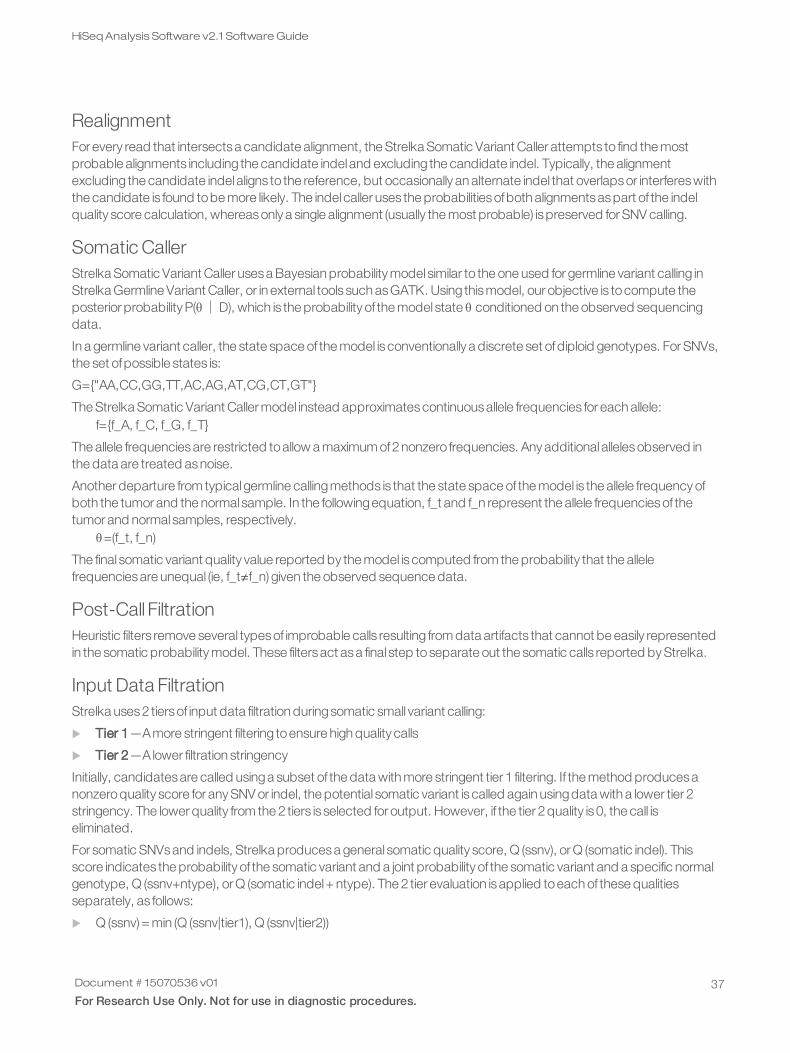
RealignmentFor every read that intersectsa candidate alignment, the Strelka Somatic Variant Caller attempts to find the mostprobable alignments including the candidate indel and excluding the candidate indel. Typically, the alignmentexcluding the candidate indel aligns to the reference, but occasionally an alternate indel that overlapsor interfereswiththe candidate is found tobe more likely. The indel caller uses the probabilitiesofboth alignmentsaspart of the indelquality score calculation, whereasonly a single alignment (usually the most probable) ispreserved for SNV calling.

Somatic CallerStrelka Somatic Variant Caller usesa Bayesian probability model similar to the one used for germline variant calling inStrelka Germline Variant Caller, or in external tools such asGATK. Using thismodel, our objective is tocompute theposterior probability P(θ│D), which is the probability of the model state θ conditioned on the observed sequencingdata.

In a germline variant caller, the state space of the model isconventionally a discrete set ofdiploid genotypes. For SNVs,the set ofpossible states is:

G={"AA,CC,GG,TT,AC,AG,AT,CG,CT,GT"}

The Strelka Somatic Variant Caller model instead approximatescontinuousallele frequencies for each allele:f={f_A, f_C, f_G, f_T}

The allele frequenciesare restricted toallow a maximum of2nonzero frequencies. Any additional allelesobserved inthe data are treated asnoise.

Another departure from typicalgermline callingmethods is that the state space of the model is the allele frequency ofboth the tumor and the normal sample. In the followingequation, f_t and f_n represent the allele frequenciesof thetumor and normal samples, respectively.

θ=(f_t, f_n)

The final somatic variant quality value reported by the model iscomputed from the probability that the allelefrequenciesare unequal (ie, f_t≠f_n) given the observed sequence data.

Post-Call FiltrationHeuristic filters remove several typesof improbable calls resulting from data artifacts that cannot be easily representedin the somatic probability model. These filtersact asa final step toseparate out the somatic calls reported by Strelka.

Input Data FiltrationStrelka uses2 tiersof input data filtration duringsomatic small variant calling:

u Tier 1—Amore stringent filtering toensure high quality calls

u Tier 2—A lower filtration stringency

Initially, candidatesare called usinga subset of the data with more stringent tier 1 filtering. If the method producesanonzeroquality score for any SNV or indel, the potential somatic variant iscalled again usingdata with a lower tier 2stringency. The lower quality from the 2 tiers is selected for output. However, if the tier 2quality is0, the call iseliminated.

For somatic SNVsand indels, Strelka producesa general somatic quality score, Q (ssnv), or Q (somatic indel). Thisscore indicates the probability of the somatic variant and a joint probability of the somatic variant and a specific normalgenotype, Q (ssnv+ntype), or Q (somatic indel+ ntype). The 2 tier evaluation isapplied toeach of these qualitiesseparately, as follows:

u Q (ssnv) = min (Q (ssnv|tier1), Q (ssnv|tier2))

Document # 15070536 v01



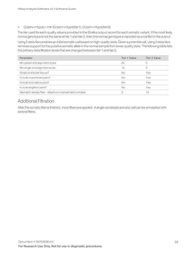
u Q (ssnv+ntype) = min (Q (ssnv+ntype|tier1), Q (ssnv+ntype|tier2))

The tier used for each quality value isprovided in the Strelka output record for each somatic variant. If the most likelynormalgenotype isnot the same at tier 1and tier 2, then the normalgenotype is reported asa conflict in the output.

Using2data tiersenablesan initial somatic call based on high-quality data. Given a potential call, using2data tiersremovessupport for the putative somatic allele in the normal sample from lower quality data. The following table liststhe primary data filtration levels that are changed between tier 1and tier 2.

Parameter Tier 1 Value Tier 2 Value

Min paired-end alignment score 20 0

Min single-end alignment score 10 0

Single-end score rescue? No Yes

Include unanchored pairs? No Yes

Include anomalous pairs? No Yes

Include singleton pairs? No Yes

Mismatch density filter—Maximum mismatches in window 3 10

Additional FiltrationAfter the somatic filter is finished, more filtersare applied. Asingle candidate somatic call can be annotated withseveral filters.

Document # 15070536 v01



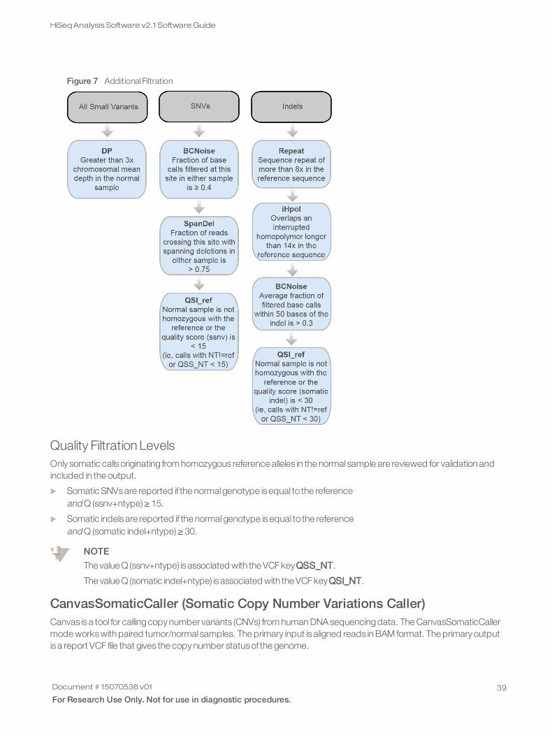
Figure 7 Additional Filtration

Quality Filtration LevelsOnly somatic callsoriginating from homozygous reference alleles in the normal sample are reviewed for validation andincluded in the output.

u Somatic SNVsare reported if the normalgenotype isequal to the referenceand Q (ssnv+ntype) ≥ 15.

u Somatic indelsare reported if the normalgenotype isequal to the referenceand Q (somatic indel+ntype) ≥ 30.

NOTE

The value Q (ssnv+ntype) isassociated with the VCFkeyQSS_NT.

The value Q (somatic indel+ntype) isassociated with the VCFkeyQSI_NT.

CanvasSomaticCaller (Somatic Copy Number Variations Caller)Canvas isa tool for callingcopy number variants (CNVs) from human DNAsequencingdata. The CanvasSomaticCallermode workswith paired tumor/normal samples. The primary input isaligned reads in BAM format. The primary outputisa report VCF file that gives the copy number statusof the genome.

Document # 15070536 v01



For more information about Canvas, see Canvason page 29or the CanvasGitHub page.

Document # 15070536 v01



https://github.com/Illumina/canvas

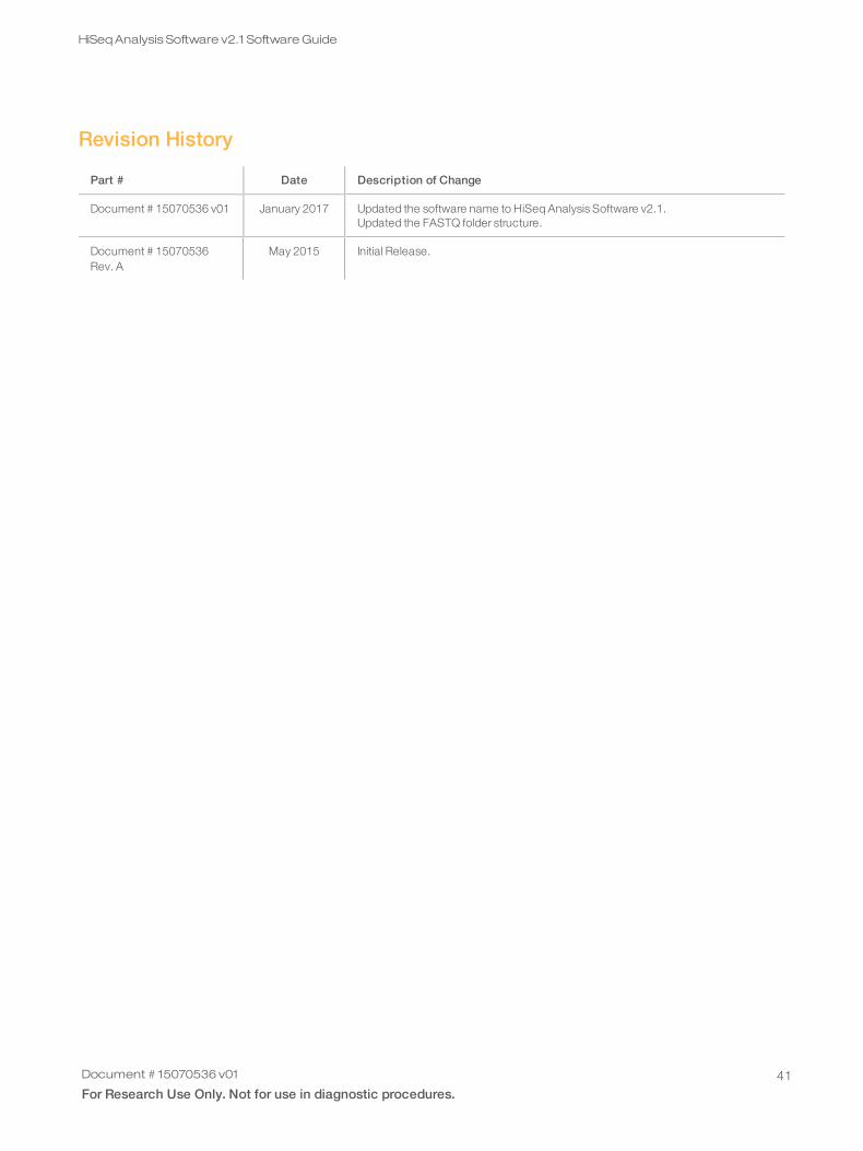
Revision History

Part # Date Description of Change

Document # 15070536 v01 January 2017 Updated the software name to HiSeq Analysis Software v2.1.Updated the FASTQ folder structure.

Document # 15070536Rev. A

May 2015 Initial Release.

Document # 15070536 v01



Technical Assistance

For technical assistance, contact Illumina Technical Support.Website: www.illumina.comEmail: [email protected]

Illumina Customer Support Telephone Numbers

North America Germany Singapore1.800.809.4566 0800.180.8994 1.800.579.2745

Australia Hong Kong Spain1.800.775.688 800960230 900.812168

Austria Ireland Sweden0800.296575 1.800.812949 020790181

Belgium Italy Switzerland0800.81102 800.874909 0800.563118

China Japan Taiwan400.635.9898 0800.111.5011 00806651752

Denmark Netherlands United Kingdom80882346 0800.0223859 0800.917.0041

Finland New Zealand Other countries0800.918363 0800.451.650 +44.1799.534000

France Norway0800.911850 800.16836

Safety data sheets (SDSs)—Available on the Illumina website at support.illumina.com/sds.html.

Document # 15070536 v01



http://www.illumina.com/

mailto:[email protected]

http://support.illumina.com/sds.html

HiSeq Analysis Software v2.1 User Guide€¦ · HiSeq Analysis Software v2.1 User Guide....

Documents

Transcript of HiSeq Analysis Software v2.1 User Guide€¦ · HiSeq Analysis Software v2.1 User Guide....