High and Low Load Sensitivities TEPPC 2024 CC Data Work Group January 27, 2015 W ESTERN E LECTRICITY...

W E S T E R N E L E C T R I C I T Y C O O R D I N A T I N G C OU N C I L

High and Low Load SensitivitiesTEPPC 2024 CC

Data Work GroupJanuary 27, 2015

2


Overview• Background Information on Running Sensitivity

Analysis• Existing Assumptions for High & Low Loads

– 10 Year Loads– 20 Year Loads

• Assumptions for Load Sensitivities– Discuss assumptions for high and low load conditions used by the California

Energy Commission– Discuss the impact of high efficiency programs on the load forecast

• Assumptions for high loads– Loads used by the ISO for Reliability Analysis– Loads used by BPA for Reliability Analysis

• Where do we go from here?

3


TEPPC\TAS Meeting 021611

• Running Sensitivities with Every Study Cycle

• DWG participants see value in running sensitivities (High and Low) with every study cycle (e.g., Gas Prices, Hydro and Loads)

• A regular schedule will give DWG and others sufficient time to prepare for getting the data and assumptions delivered on time.

• The question about submitting an associated study request to TEPPC been settled by Brad. The request is internal to the TEPPC process and should be settled as such.

4

• Already planning to run low load and high DSM sensitivitiesoNo consideration been given to run high load

sensitivity.

• The LRS loads are one in two year risk exposure, whereas, transmission planning is typically performed with one in five and one in ten.

• TEPPC planning is transmission planning.

TEPPC\TAS 013012DWG report on Load Sensitivities:

5


Existing Assumptions for High & Low Dan Beckstead, WECC

6


Assumptions for High & Low Load Conditions Angela Tangahetti, CEC

7


Introduction

Topics to Cover:

• Developing CEC IEPR “Common Cases”• Overview of Common Case Methodology• Common Case Input Assumptions

8


Purpose of IEPR “Common Cases”

• Energy sectors serving California are complex, interdependent systems lead to three common cases that “easily” translate across sector

• Lack of common case assumptions led to sectors “fractured” analytical approaches

• Stronger analytical basis for policy discussions

9


Common Cases Require Common Definitions

• Defining cases key to coordination• “High” & “Low” not specific enough • Three worldviews chosen to model

• Reference/Mid Case or Business as Usual• High Energy Consumption• Low Energy Consumption

Graphical Representation of Iterative Modeling Process

WECC Electricity Dispatch Model North American

Gas Model

Updated Economic/

Demographic Assumptions

CA Transportation

Demand Models

CA Electricity Demand Models

WECC Electricity Dispatch Model

Common Case Input Assumptions

• Gross Domestic Product Growth • CPI Inflation• Gross State Product• Population Growth• Energy Efficiency Improvements• Demand Response• Carbon Prices • Weather (HDD/CDD)

Trade-Offs in High and Low Energy Consumption Cases

• High and Low Consumption Scenario for one sector comes at expense of other sectors

• Some trade-offs necessary in defining high and low cases

• Chosen approach was “Major Driver” testIf input value was major driver in one model

but not others, value set by model where major driver

Resolution of Conflicting Variables

Variable• Electricity Price• NG Price• Crude Oil Price• EV Penetration• Coal Price• NGV Penetration

Controlling Model• Electricity• Natural Gas• Transportation• Transportation• Electricity• Transportation

Understanding Case Development

• Reference/Mid Case reasonably expected trajectory given best available input

• High and Low Cases Energy Consumption cases are reasonable range

• High and Low Cases Energy Consumption are NOT most extreme possible

High and Low Common Case AssumptionsRelative to Mid/Reference Case

Input Category High Demand Low Demand

Natural Gas Electricity Transportation Natural Gas Electricity Transportation

GDP High High High Low Low Low

Wholesale Electricity Price Low Low High High High Low

Retail Electricity Rates Low Low High High High Low

NG Supply Cost Low Low High High High Low

Crude Oil Price High No Effect Low Low No Effect High

Pop/Demographics High High High Low Low Low

Renewables (Gen) Low High High High Low Low

Energy Efficiency Low Low No Effect (High) High High No Effect (High)

Demand Response Low Low No Effect (High) High High No Effect (High)

CHP Low Low No Effect (High) High High No Effect (High)

Carbon Price Low Low Low High High High

Weather (HDD/CDD) High High No Effect Low Low No Effect

Low Carbon Fuel Standard High High Low Low Low High

Electric Vehicle Penetration High High Low Low Low High

Ren. Fuel Vehicles No Effect No Effect Low No Effect No Effect High

CAFÉ Standards No Effect No Effect Low No Effect No Effect High

Coal Price Low Low No Effect (Low) High High No Effect (High)

Notes For Chart on Previous Slide

• Terminology - "High" and "Low" case metrics is demand/consumption

• High - Represents a value above those identified in the Mid Case • Low - Represents a value below those identified in the Mid Case • Highlighted cells represent values which have a conflict between

what settings the modeling teams would each use• Parentheticals represent theoretical setting if the model allowed it.

Actual values are outside parenthesis and represent limitations of model complexity or setting.

• Major/Minor drivers - Not all models are strongly sensitive to all of these factors. The goal is to identify which models see these inputs as "Major" drivers and use those models to determine which of these values should be used for the common cases.

17


The Impact of High Efficiency Programs on the Load Forecast

Galen Barbose, LBNL

2022 High DSM Case

• Assume “all cost-effective EE potential” is achieved throughout the West– Intended as a boundary case– Agnostic about what types of policies are used to get there

(codes, standards, customer-funded programs, etc.)• Rely on recent existing EE potential studies to estimate

potential for individual utilities/regions – Extrapolate to regions for which recent potential studies are

unavailable– Lots of complexities (e.g., differences in study vintage/scope,

baseline definition, etc.) and approximations

18

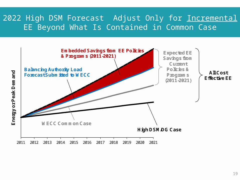
2022 High DSM Forecast Adjust Only for Incremental EE Beyond What Is Contained in Common Case

19

2011 2012 2013 2014 2015 2016 2017 2018 2019 2020 2021

En

erg

y o

r P

ea

k D

em

an

d

WECC Common Case

All Cost Effective EE

High DSM/DG Case

Balancing Authority Load Forecast Submitted to WECC

Embedded Savings from EE Policies & Programs (2011-2021)

Expected EE Savings from

Current Policies & Programs

(2011-2021)

2022 WECC-Wide EE ImpactsCommon Case vs. High DSM Case

20

GWh MW

Cumulative Savings (2011-2021)Common Case 112,466 24,874High DSM Case 203,525 43,592

Cumulative Savings (% of 2021 Load)Common Case 10.2% 11.5%High DSM Case 18.4% 20.1%

CAGR (2010-2021)Common Case 1.4% 1.3%High DSM Case 0.5% 0.3%

• Common Case EE savings represent roughly 10% of total WECC-wide load• High DSM Case represents roughly an additional 8% reduction in WECC-

wide annual energy and 9% reduction in non-coincident peak

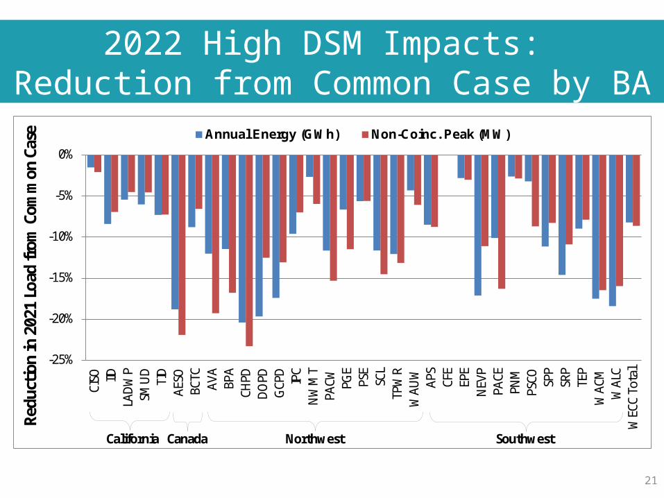
2022 High DSM Impacts: Reduction from Common Case by BA

21

-25%

-20%

-15%

-10%

-5%

0%

CISO IID

LADW

PSM

UD

TID

AESO

BCTC

AVA

BPA

CHPD

DOPD

GCP

DIP

CN

WM

TPA

CW PGE

PSE

SCL

TPW

RW

AUW

APS

CFE

EPE

NEV

PPA

CEPN

MPS

CO SPP

SRP

TEP

WAC

MW

ALC

WEC

C To

tal

Annual Energy (GWh) Non-Coinc. Peak (MW)

California Canada Northwest Southwest

Redu

ction

in 2

021

Load

from

Com

mon

Cas

e

2032 High DSM Case

• Partnered with Itron to apply their Statistically Adjusted End-Use (SAE) load forecasting framework– Econometric model with stock efficiency and saturations specified for

30 separate end-uses– Produces monthly energy and peak demand, disaggregated by end-use

• Key Efficiency Assumption for High DSM Forecast: Average stock efficiency for each end-use reaches level equivalent to the most efficient models commercially available today

• Requires a structured sequence of load forecasts• Calibrated to the official WECC Reference Case

22

2032 High DSM ImpactsReduction from Reference Case

23

• Roughly 20% reduction in WECC-wide annual energy in 2032, relative to reference case

• Variation across states reflects differences in end-use mix, reference case efficiency level, weather, etc.

-30.0%

-25.0%

-20.0%

-15.0%

-10.0%

-5.0%

0.0%

AESO

APS

AVA

BCTC

BPA

CFE

CHPD

DO

PDEP

EFA

R_EA

STG

CPD

IID LDW

PM

AGIC

_VLY

NEV

PN

WM

TPA

CE_I

DPA

CE_U

TPA

CE_W

YPA

CWPG

E_BA

YPG

E_VL

YPG

NPN

MPS

CPS

ESC

ESC

LSD

GE

SMU

DSP

PSR

PTE

PTI

DC

TPW

RTR

EAS_

VLY

WAC

MW

ALC

WAU

WW

ECC

High DSM Case Incremental Savings: Percentage Reduction from SAE Reference Case (2032)

Annual EnergyNon-Coincident Peak

24


A Few Take-Aways and Questions to Consider

• Increasing or decreasing EE by 50% relative to what is embedded in Common Case forecast is equivalent to about a +/- 5% adjustment in total WECC-wide loads over 10 years

• Prior high DSM study cases suggest aggressive EE alone could reduce loads by almost 10% over 10 years, compared to Common Case– Is an aggregate 10% reduction for Low Load Sensitivity too modest, given

additional potential drivers for low load beyond EE?• EE impacts differ greatly by load zone (e.g., 2-20% of load)

– Is a one-size-fits-all 10% reduction for the Low Load Sensitivity too coarse; are region- or BA-specific adjustments warranted?

• EE impacts on peak demand are not proportional to energy impacts, but perhaps close enough for level of precision desired

25


Loads Used by the CAISO for Reliability AnalysisIrina Green, CAISO

26


Load Forecast for Annual Transmission Planning Process (TPP)

• CEC Load forecast is used as the starting point

– For 2014-2015 TPP, the mid-case California Energy Demand Forecast 2014-2024 released by California Energy Commission (CEC) dated January 2014 with the Mid-Case LSE and Balancing Authority Forecast spreadsheet updated as of February 8, 2014.

– Energy Efficiency Adjustments based on 2013 IERP final report from January 23, 2013

Using Mid Additional Achievable Energy Efficiency scenario

• http://www.energy.ca.gov/2013_energypolicy/documents/demand-forecast_CMF/Additional_Achievable_Energy_Efficiency/January_2014_files/

http://www.energy.ca.gov/2013_energypolicy/documents/demand-forecast_CMF/Additional_Achievable_Energy_Efficiency/January_2014_files/



27


Load Forecast (continued)

• Methodologies used by Participating Transmission Owners (PTOs) to create bus-level load forecast are documented in the Study Plan

• 1-in-10 year heat wave load projection for individual local area studies

• 1-in-5 year heat wave load projection for bulk system studies• PTOs subtract losses from the CEC forecast• Pumping loads are modeled as generators with negative output• CAISO studies summer peak, summer off-peak, minimum load

cases, winter peak cases for some areas, and other cases as needed (spring peak, summer partial peak)

28


Study Areas

Northern Area: PG&E – bulk system and local areasSouthern area:SCE, SDG&E, VEA

29


Load Forecast MethodologyPG&E

• PG&E creates bus-level load forecast (using CEC forecast as the starting point)– PG&E loads in the base case

• Determination of Division Loads based on historical data and projected load growth.

• Total PG&E load growth allocated to divisions and adjusted based on 1-in-10 or 1-in-5 temperatures

• Allocation of Division Load to Transmission Bus Level depending on types of loads: conforming, non-conforming, self generation and plant (not included in division loads)

• Municipal loads in the base case – municipal utilities provide their load forecast to PG&E

30


Load Forecast MethodologySCE

31


Load Forecast MethodologySDG&E

• Utilize CEC’s latest load forecast as the starting point

• SDGE’s methodology to create bus-level load forecast

– Actual peak loads on low side of each substation bank transformer from historical data

– Normalizing factors applied for achieving weather normalized peak

– Adverse temperature adjustment factor applied to get the adverse peak

– Adverse load and coincident load determined for each substation

32


Load Forecast MethodologyValley Electric (VEA)

• Historical SCADA data and load plans• Adjusted to CEC forecast

33


• Questions?• Comments?

• Irina Green [email protected] 916-608-1296

mailto:[email protected]

34


Loads Used by the BPA for Reliability Analysis

Reed Davis, BPA

BPA’s Transmission System

35

36

BPA’s methodology to create BUS forecasts

• Historical data used to create monthly energy and peak forecasts

• Weather normalizing factors included as appropriate

• Forecasted with a 34 year average peak producing temperature. Considered a 1 in 2 peak. Temperatures are updated every 10 years.

• Forecasts reviewed with local utility staff to make sure it aligns with local construction plans.

• New large loads are reviewed and added directly to forecast if load has a greater than 70% chance of occurring.

• Permanent load transfers between BUS are included.

• Specific large conservation projects are included directly at the BUS level.

37

BPA’s methodology for special BUS forecasts

• Using the base BUS forecast we – Adjust to 1 in 20 weather conditions

– Add economic uncertainty based on economic conditions surrounding the BUS and load delivery over the BUS based on load type: conforming, non-conforming.

– Adjust for changing conservation plans

38


High and Low Load Sensitivities TEPPC 2024 CC Data Work Group January 27, 2015 W ESTERN E LECTRICITY...

Documents

Transcript of High and Low Load Sensitivities TEPPC 2024 CC Data Work Group January 27, 2015 W ESTERN E LECTRICITY...