Hedging in the Possible Presence of Unspanned

Stochastic Volatility:

Evidence from Swaption Markets∗

Rong Fan† Anurag Gupta‡ Peter Ritchken§

August 13, 2002

∗The authors would like to thank seminar participants at presentations made at the Twelfth Annual Derivatives

Securities Conference in New York, The 2002 FMA European Meetings in Copenhagen, the Seventh Annual US

Derivatives and Risk Management Congress in Boston, The 2002 Western Finance Association Meetings in Park

City, The Second World Congress of the Bachelier Finance Society in Crete, and Georgetown University. They

also acknowledge support for this research from the Federal Reserve Bank in Cleveland.†Case Western Reserve University, WSOM, 10900 Euclid Ave., Cleveland, OH 44106-7235, Phone: (216)

368–3849, Fax: (216) 368–4776, E-mail: rxf10@po.cwru.edu‡Case Western Reserve University, WSOM, 10900 Euclid Ave., Cleveland, OH 44106-7235, Phone: (216)

368–2938, Fax: (216) 368–4776, E-mail: axg77@po.cwru.edu§Case Western Reserve University, WSOM, 10900 Euclid Ave., Cleveland, OH 44106-7235, Phone: (216)

368–3849, Fax: (216) 368–4776, E-mail: phr@po.cwru.edu

Hedging in the Possible Presence of Unspanned Stochastic Volatility:

Evidence from Swaption Markets

Abstract

This paper examines whether higher order multifactor models, with state variables linked solelyto the full set of underlying LIBOR-swap rates, are by themselves capable of explaining and hedg-ing interest rate derivatives, or whether models explicitly exhibiting features such as unspannedstochastic volatility are necessary. Our research shows that swaptions and even swaption strad-dles can be well hedged with LIBOR bonds alone. We examine the potential benefits of lookingoutside the LIBOR market for factors that might impact swaption prices without impactingswap rates, and find them to be minor, indicating that the swaption market is well integratedwith the underlying LIBOR-swap market.

JEL Classification: G12; G13; G19.

Keywords: Interest Rate Derivatives; Swaptions; Delta and Gamma Neutral Hedging; Un-spanned Stochastic Volatility; Spanning.

Understanding the dynamics of the term structure of interest rates is crucial for pricing andhedging fixed income positions. It is therefore not surprising that this subject continues to attractkeen interest. In the last decade, researchers have focused their attention on term structuremodels where the yield to maturity is an affine function of the underlying state variables.1 Theempirical literature has evolved from studying one-factor diffusions to multi-factor models thatincorporate stochastic central tendency, stochastic volatility, jumps, and non trivial correlationsamong state variables. With respect to derivatives, Chacko and Das (2002) show that there arecomputational advantages in pricing certain claims in the affine class, where simple solutionsoften exist.

Recently, several authors have identified limitations of affine models.2 Jagannathan, Kaplinand Sun (2001) investigate whether these limitations are severe enough to affect their use invaluing interest rate claims. In particular, they estimate one, two and three-factor Cox, Ingersolland Ross (1985) models and show that as the number of factors increases, the fit of the modelto LIBOR and swap rates improves. However, when they use their estimated models to priceswaptions, the pricing errors are biased and large. They conclude that while more factors mightbe necessary to explain swaption prices, it might be useful to investigate alternative structures,possibly outside the affine class. Their findings also point out the need for evaluating termstructure models using data on derivative prices.

The Jagannathan, Kaplin, and Sun study uses time series information on LIBOR and swaprates to estimate models under the data generating measure. An alternative approach is touse a set of observable derivative prices to directly calibrate the parameters of a model underthe risk neutral pricing measure and then analyze any systematic biases in the pricing errors.This process was followed by Longstaff, Santa Clara and Schwartz (2001)(hereafter LSS), amongothers.3 They use observable swaption prices to extract information on volatility structures forforward rates, and conclude that in order to price swaptions effectively, models with three or fourfactors are necessary. However, they find that models calibrated using swaption data producetheoretical cap prices that often deviate significantly from the no-arbitrage values implied bythe swaptions market. Their results indicate that the swaption and cap markets may not bewell integrated, or that their models do not capture all elements of risk.

1Duffie and Kan (1996) link these models to the affine structure of the underlying stochastic processes of the

state variables, and Dai and Singleton (2000) identify the maximally flexible affine models, that, from an empirical

perspective, nest all other affine models.2For example, see Backus, Foresi, Mozumdar and Wu (2001), Ghysels and Ng (1998), and Duffee (2002). Ahn,

Dittmar and Gallant (2002) develop a family of quadratic term structure models that nest several existing models,

including the SAINTS model of Constantinides (1992) and the double square root model of Longstaff (1989), and

provide empirical support that their models outperform affine models in explaining historical bond price behavior

in the United States.3Hull and White (1999) develop very similar models to the LSS models using the LIBOR market based model

of Brace, Gatarek and Musiela (1997).

1

The possible lack of integration between price behavior in related markets, such as thecap and swaption markets, could arise from the fact that derivative prices may be affectedby factors outside the LIBOR bond market. If this is the case, then the swap markets areincomplete and hence there is no reason for the variance-covariance matrix of forward rates,implied out from cap and swaption data, to be similar to the variance-covariance matrix impliedfrom interest rates. Indeed, De Jong, Driessen and Pelsser (2002) show that the historicalcorrelations are significantly higher than those implied from cap and swaption data using afull-factor lognormal market model. One of their explanations is that a volatility risk premiummay be present. Heidari and Wu (2001) show that less than 60% of the variation in swaptionvolatilities can be explained by the three common interest rate factors identified by Littermanand Scheinkman (1991). In addition to the level, slope and curvature of the yield curve, theyidentify three additional volatility related factors, independent of interest rate factors, thatincrease the explained variability of swaption volatilities to over 95%. They use this evidence tosuggest that swaptions cannot be hedged using LIBOR state variables alone.

Other studies have also confirmed the lack of integration between prices in related markets.Collin-Dufresne and Goldstein (2002) regress the returns on at-the-money cap straddles, whichare portfolios mainly exposed to volatility risk, against changes in swap rates drawn from acrossthe yield curve. On average, over all contracts, they find that the swap rate changes onlyexplain about 25% of the straddle returns. Further, the residuals of these regressions are highlycorrelated over the different contracts, and a principal component analysis indicates that about85% of the remaining variation can be explained by a single common factor. They concludethat there is at least one state variable which drives innovations in interest rate derivatives,but which does not affect innovations in LIBOR-swap rates. In other words, they suggest thatcaps cannot be priced relative to bonds alone, or equivalently, that the bond market by itself isincomplete. They term this feature unspanned stochastic volatility, and establish models withinan appropriately curtailed trivariate Markov affine system that display this interesting property.Han (2001) establishes a term structure model that explicitly models the covariances of bondyields as being linear in a set of state variables. In his model, the two factors for covariances canbe viewed as a level dependent and a slope dependent factor for the term structure of volatilities.Han finds empirical support for this model.

The above studies all suggest that there are sources of risk that affect fixed income derivativeswhich cannot be effectively hedged by portfolios consisting solely of LIBOR bonds or swaps, andthat the set of hedging instruments may have to be broadened, possibly to include some options.Our paper investigates the relative importance of these other sources of risk in the swaptionmarket. In particular, if unspanned stochastic volatility is important, then it should not bepossible to hedge swaptions effectively using a model based on state variables limited to the setof swap rates. More importantly, such models should certainly not be able to hedge contracts

2

which have extreme sensitivity to volatilities, such as straddles. If a model can be identified inwhich the entire matrix of swaptions and their straddles can be well hedged by bonds, then theneed to explicitly incorporate additional factors that influence swaptions but not swaps appearsto be minor. On the other hand, if swaptions cannot be well hedged, then either the modelsare misspecified or indeed there are other factors, beyond the term structure, that influence thebehavior of swaption prices.

We construct simple multifactor models that hedge swaptions and swaption straddles veryeffectively, and, based on the empirical performance of these hedges, we conclude that thebenefits of explicitly incorporating unspanned stochastic volatility into models are minor.

Our paper examines the importance of multifactor models from the perspective of hedgingeffectiveness. In contrast, most of the other studies focus on pricing performance.4 For example,LSS use pricing accuracy as the criterion to conclude that four factors are necessary for pricingswaptions. However, the number of free parameters in their models equals the number of factors.As a result, it is unclear whether the improvement in pricing is attributable to the number offactors or to the number of free parameters. Indeed, when we redo their pricing tests on our datawe reconfirm their findings. In particular, we find significant improvements in pricing accuracywhen incorporating up to four factors. However, it is easy to construct a one-factor model,containing the same number of parameters as their four-factor model, that prices swaptionsequally well.

Unfortunately, a pricing analysis, even conducted out-of-sample, tells us little about the truevolatility structure of forward rates. It therefore does not assist us in understanding the trueimportance of multiple factors and the real capability of a model. In contrast, our study carefullyevaluates models in terms of hedging precision. If a continuous time model is correct, the riskof carrying a hedged position over a time increment is entirely due to the fact that the volatilityparameters are not estimated precisely and continuous revisions are not accomplished. If onemodel consistently produces hedges that are more effective than another model, then it mustbe the case that the first model, with its volatility structure, better captures the true dynamicsof the term structure and the true sensitivity of options to movements in the underlying termstructure. Not only do we consider the effectiveness of multi-factor delta neutral hedges, but,for the case of high gamma positions such as straddles, we also investigate the effectiveness ofdelta and gamma neutral hedges. To our knowledge, this is the first study to investigate theconsequences of adopting these hedge strategies using one, two, three and four-factor models inwhat is unquestionably a multifactor environment.

The paper proceeds as follows. In section 1, we describe the models that we evaluate, thedata, and the experimental design. In section 2, we examine the ability of different models in

4For exceptions to this rule see Driessen, Klaassen, and Melenberg (2001) and Gupta and Subrahmanyam

(2001).

3

hedging swaptions. From a hedging perspective, the dangers in using lower order models areclearly revealed, and the benefits of using higher order models become apparent. In section 3, weaddress spanning issues in the swaption market. It is common to frequently recalibrate a modelto observed option prices. This process may compensate for the inability of the model to capturethe true term structure dynamics. Specifically, in the presence of unspanned stochastic volatility,the recalibrating process could incorporate swaption price information into a model that is basedon swap rate state variables alone and mask the presence of missing state variables. In ouranalysis, we address this issue by measuring the hedging effectiveness when model recalibrationsare not permitted. We analyze volatility sensitive straddles, which are hedged to be delta andgamma neutral. These hedges, maintained for one week, can explain about 85% of the unhedgedvariance. In contrast, when simply regressing swaption straddle returns on swap rate changes,we obtain R2 values near 15%, comparable to the results Collin-Dufresne and Goldstein (2002)obtained for cap straddles. The consequences of our findings are explored. Section 4 concludes.

1 Models, Data, and Experimental Design

1.1 The Basic Models

Swaptions are actively traded, and, according to market convention, their prices are quoted involatility form using the standard Black (1976) model, with instruments at different expirationdates, underlying swap maturities and strikes trading at different implied volatilities. The Blackformula should be viewed only as a nonlinear transformation from prices into volatilities andvice-versa. This market convention provides a convenient way of communicating prices becausevolatilities tend to be more stable over time than actual dollar prices. The market conventiondoes not imply that participants in this market view the Black model as being appropriate.

Let f(t, T ) denote the forward interest rate at time t for instantaneous riskless borrowing orlending at date T. The dynamics of forward rates are given by

df(t, T ) = µf (t, T )dt +N∑

n=1

σfn(t, T )dwn(t), with f(0, s) given for s ≥ 0. (1)

where {dwn(t)|n = 1, 2, . . . , N} are standard independent Wiener increments. The volatilitystructures, {σfn(t, T )|n = 1, 2, . . . , N}, could, in general, be functions of all path information upto date t.

Heath Jarrow and Morton (1992) show that to avoid riskless arbitrage, the drift term, underthe equivalent martingale measure, is completely determined by the volatility functions in the

4

above equation. Specifically:

µf (t, T ) =N∑

n=1

σfn(t, T )∫ T

tσfn(t, u)du.

This implies that for pricing purposes, only the volatility structures need to be specified andestimated. The structures that we use are based on the loadings provided by the principalcomponents of the historical correlation matrix of forward rates along the lines of the stringmodels of LSS. In these models we consider a discrete set of M maturities say, {τ1, τ2, . . . , τM}with τ1 < τ2, . . . , τM . Then:

σfj(t, t + τj) = g(τj)f(t, t + τj) (2)

where g(.) is a deterministic function of the maturity of the forward rate, that is estimated usingthe principal components extracted from the historical correlation matrix of weekly forward ratepercentage changes. These forward rates are separated by three months for maturities less thana year, and six months thereafter (for up to ten years maturity). Specifically, twenty two forwardrate maturities are used and a twenty two by twenty two correlation matrix is established. Thematrix of eigenvectors (principal components) is computed, and the first four eigenvectors areretained. Let

T ∗ = {τ1 = 0.25, τ2 = 0.5, τ3 = 0.75, τ4 = 1, τ5 = 1.5, τ6 = 2, τ7 = 2.5, ...τ21 = 9.5, τ22 = 10}

represent the set of 22 forward rate maturities, and let hi be a 22× 1 vector representing the ith

eigenvector for i = 1, 2, 3 and 4. Then, define:

gi(τj) = λihij. where i = 1, 2, 3, 4 and j = 1, 2, ..., 22.

where hij is the jth element of the ith eigenvector, and the λi values are the free parameters, theith one representing the scaling factor for all the elements of the ith principal component, andis implied out at any date t using date t swaption data.

The principle behind such a procedure is simple. As shown by several researchers, includingLitterman and Scheinkman (1991), the first four historical principal components identify thefour most important types of orthogonal shocks to the forward rate curve. Since the exactcontribution of each of these shocks may vary over time, the eigenvalues for the future periodmay be different from the eigenvalues over the historical period. Since, in an efficient market,the swaption data reflects all available information on the set of forward looking correlationsamong forward rates, this data should be used to establish the eigenvalues.

The above method, which we term an adapted Principal Component Analysis method hasbeen used by LSS for models where forward rate volatilities are proportional to their levels, andby Driessen, Klaassen and Melenberg for models where forward rate volatilities do not dependon their levels.

5

1.2 Data

The data for this study consists of volatilities of USD swaptions of expiration 6 months, 1-, 2-,3-, 4-, and 5-years, with the underlying swap maturities of 2-, 3-, 4, and 5-years each (in all, thereare 24 swaption contracts). As per market convention, a swaption is considered at-the-moneywhen the strike rate equals the forward swap rate for an equal maturity swap. The data consistsof volatilities of at-the-money contracts over a 32 month period (March 1, 1998 - October 31,2000), obtained from DataStream. Figure 1 presents the time series of implied Black volatilitiesfor swaptions over the sample period.

Figure 1 Here

Each of the graphs corresponds to a time series for all swaption expirations for each underly-ing swap maturity. The figure clearly shows the changing variances over this time period, withthe peaks occurring during the Long Term Capital Management crisis. Table 1 provides thetime series properties for each of the contracts. The range of volatilities is largest for the shortterm contracts. The last column of the table indicates the typical bid-ask spread for each of thecontracts. The typical bid-ask spread over this time period was approximately plus or minus ahalf Black vol. The spreads, in basis points, were obtained by repricing the swaption using theBlack model, first with a volatility that exceeded the mean by 0.5 Black vols, and then witha volatility 0.5 units below the mean. These numbers indicate the coarseness of the data andserve as a benchmark for evaluating hedging precision.

Table 1 Here

For constructing the yield curve, we use futures and swap data. For the short end of thecurve (up to 1 year maturity), we use the five nearest futures contracts on any given data. Thesefutures rates are interpolated, and then convexity corrected to obtain the forward rates for 3,6, 9, and 12-month maturities. The rest of the yield curve out to 5 years is estimated using theforward rates bootstrapped from market swap rates at 6 month intervals. The futures and swapdata is obtained from DataStream. Eventually, we obtain weekly forward rate curves that startone year before our swaption data begins, and extend to the end of our swaption data period.

For the principal component analysis we use the one year history of forward rates that existsprior to the beginning of our swaption data, to estimate the correlation structure of forward rates.We then decompose the correlation matrix, R, into UΛ∗U ′, where U is the matrix of eigenvectorsand Λ∗ is a diagonal matrix of eigenvalues. Finally, we retain the first four eigenvectors andassume a covariance structure for forward rates, Σ, given by Σ = UΛU ′ where Λ is a diagonalmatrix with the first four diagonal elements positive, the others zero.

6

1.3 Model Implementation

We consider a discrete implementation of the multifactor HJM model. Towards this goal, wedivide the time interval into trading intervals of length ∆t, and label the periods with consecutiveintegers. Let f∆t(t, j) be the forward rate at period t, for the time interval [j∆t, (j +1)∆t]. Let∆f∆t(t, j) represent the change in the forward rate over a time increment ∆t. That is

∆f∆t(t, j) = f∆t(t + 1, j) − f∆t(t, j)

The actual magnitude of this change could depend on the forward rate itself, its maturity date,and other factors.

We start with an initial forward rate curve, {f∆t(0, j), j = 0, 1, . . . ,m} that is chosen tomatch the observed term structure at date 0 for all maturities up to date m∆t. Notice thatf∆t(0, 0) is just the spot rate for the immediate period, [0,∆t]. Over each time increment, theforward rates change as follows:

∆f∆t(t, j) = µ∆tf (t, j)∆t +

N∑n=1

σ∆tfn

(t, j)√

∆tZ(n)t+1. (3)

where Z(n)t+1 is a standard normal random variable, j is an integer larger than the current

date, t, µ∆tf (t, j) is the drift term, and σ∆t

fn(t, j), is the volatility term associated with the nth

factor, n = 1, 2, ..., N , where the N standard normal random variables are independent. Thediscrete time equivalent of the Heath-Jarrow-Morton restriction is given by

µ∆tf (t, j) =

N∑n=1

µ∆tfn

(t, j)

whereµ∆t

fn(t, j) = σ2 ∆t

fn(t, j)

∆t

2+ σ∆t

fn(t, j)σ∆t

pn(t, j)

and

σ∆tpn

(t, j) =j−1∑

i=t+1

σ∆tfn

(t, i)∆t

for n = 1, 2, ...., N .

Prices of European interest rate claims can be computed using Monte Carlo simulation.Specifically, assume K different paths, are simulated, each path initiated at date 0 where theinitial term structure is given. Consider the kth simulation. Given the date 0 term structure,forward rates are updated recursively using equation (3). This gives the kth path of the termstructure of forward rates. At date 0, $1.0 is placed in a fund that rolls over at the short rate.At date T∆t the value of the money fund, M(T ; k), is given by:

M(T ; k) =T−1∏i=0

ef∆t(i,i)∆t.

7

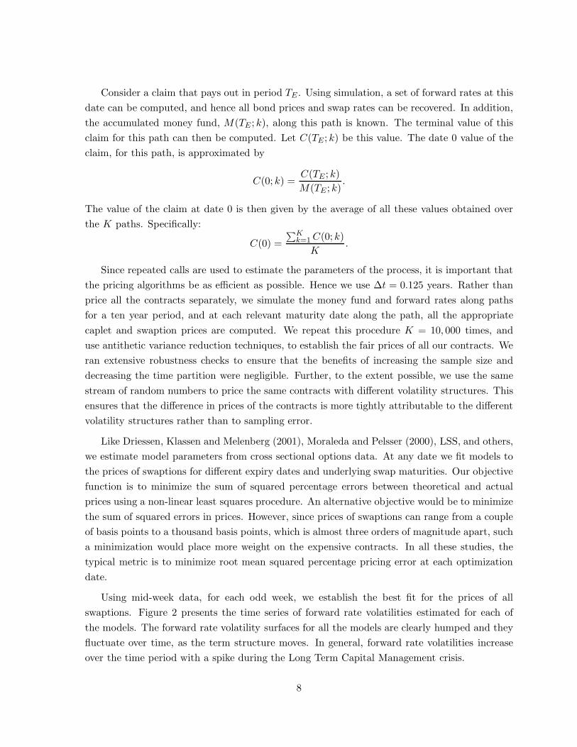
Consider a claim that pays out in period TE . Using simulation, a set of forward rates at thisdate can be computed, and hence all bond prices and swap rates can be recovered. In addition,the accumulated money fund, M(TE ; k), along this path is known. The terminal value of thisclaim for this path can then be computed. Let C(TE; k) be this value. The date 0 value of theclaim, for this path, is approximated by

C(0; k) =C(TE ; k)M(TE ; k)

.

The value of the claim at date 0 is then given by the average of all these values obtained overthe K paths. Specifically:

C(0) =∑K

k=1 C(0; k)K

.

Since repeated calls are used to estimate the parameters of the process, it is important thatthe pricing algorithms be as efficient as possible. Hence we use ∆t = 0.125 years. Rather thanprice all the contracts separately, we simulate the money fund and forward rates along pathsfor a ten year period, and at each relevant maturity date along the path, all the appropriatecaplet and swaption prices are computed. We repeat this procedure K = 10, 000 times, anduse antithetic variance reduction techniques, to establish the fair prices of all our contracts. Weran extensive robustness checks to ensure that the benefits of increasing the sample size anddecreasing the time partition were negligible. Further, to the extent possible, we use the samestream of random numbers to price the same contracts with different volatility structures. Thisensures that the difference in prices of the contracts is more tightly attributable to the differentvolatility structures rather than to sampling error.

Like Driessen, Klassen and Melenberg (2001), Moraleda and Pelsser (2000), LSS, and others,we estimate model parameters from cross sectional options data. At any date we fit models tothe prices of swaptions for different expiry dates and underlying swap maturities. Our objectivefunction is to minimize the sum of squared percentage errors between theoretical and actualprices using a non-linear least squares procedure. An alternative objective would be to minimizethe sum of squared errors in prices. However, since prices of swaptions can range from a coupleof basis points to a thousand basis points, which is almost three orders of magnitude apart, sucha minimization would place more weight on the expensive contracts. In all these studies, thetypical metric is to minimize root mean squared percentage pricing error at each optimizationdate.

Using mid-week data, for each odd week, we establish the best fit for the prices of allswaptions. Figure 2 presents the time series of forward rate volatilities estimated for each ofthe models. The forward rate volatility surfaces for all the models are clearly humped and theyfluctuate over time, as the term structure moves. In general, forward rate volatilities increaseover the time period with a spike during the Long Term Capital Management crisis.

8

Figure 2 Here

The implied correlations produced by the models are quite different from one another. Thecorrelations among rates for the models generally decrease as the number of factors increase,with the four-factor model producing correlations that typically are the closest to the historicalcorrelations. For example, the average correlations of the short 6 month rate with the 5 and 10year six-month forward rates are 0.689 and 0.410 respectively, while the historical values were0.695 and 0.370.5

2 Hedging Performance of Swaption Models

Our hedging experiments were conducted as follows. Given any calibrated n-factor model, wecan establish a hedge position for a particular swaption using n different LIBOR discount bonds.For example, for a four-factor model, four price changes for each swaption are recorded, eachprice change arising after a small shock is applied to a single factor. In addition, the four pricechanges to a set of discount bonds are computed. The unique portfolio of the four bonds is thenestablished that hedges the swaption against instantaneous shocks consistent with the model.The construction of the hedged position at any date t, only uses information available at date t.This analysis is repeated for all contracts and for all models. The hedge position is maintainedunchanged for one week, and the hedged and unhedged residuals are obtained and stored. Wethen repeat this analysis for holding periods of two, three and four weeks.

Unfortunately, one week later, the prices of the old swaptions are unavailable, so the rawresiduals of the unhedged positions cannot be directly observed. These prices, however, can beestimated using the observed set of fresh at-the-money swaption prices. We assume that the newvolatility of each old swaption equals the volatility of the new at-the-money contract. Implicitin this analysis is the assumption that the volatility skew effect is insignificant over the regionof strike price changes during a week. Indeed, we find that in more than 90% of the data, thestrike changes by less than 30 basis points over a week, and in more than half the cases, thechange is less than 10 basis points. Therefore, we really only require that contracts, with strikeswithin 30 basis points of the at-the-money contracts, have the same Black vols.6 In contrast tothe swaptions, the change in value of the bonds in the hedge portfolio is directly observable.

5For a detailed empirical investigation of the relationship between historical correlations and implied corre-

lations, see De Jong, Driessen and Pelsser (2002). Additional discussions on the importance of matching model

correlations to historical correlations is provided by Collin-Dufresne and Goldstein (2002b), Han (2001), LSS,

Radhakrishnan (1998), Rebonato (1999), and others.6LSS use the exact same procedure to compute the value of one week old swaptions, and conduct a variety of

tests to indicate the viability of this procedure. Other studies that adopt the same assumptions include Driessen,

Klaassen and Melenberg (2001) and Moraleda and Pelsser (2000). Until reliable prices of away-from-the-money

swaptions are available, there is no objective way to adjust the Black vols. for any possible strike price bias.

9

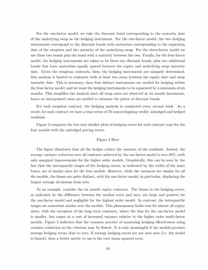
For the one-factor model, we take the discount bond corresponding to the maturity dateof the underlying swap as the hedging instrument. For the two-factor model, the two hedginginstruments correspond to the discount bonds with maturities corresponding to the expirationdate of the swaption and the maturity of the underlying swap. For the three-factor model weuse these two bonds plus the bond with a maturity between the two. Finally, for the four-factormodel, the hedging instruments are taken to be these two discount bonds, plus two additionalbonds that have maturities equally spaced between the expiry and underlying swap maturitydate. Given the swaption contracts, then, the hedging instruments are uniquely determined.Our analysis is limited to contracts with at least two years between the expiry date and swapmaturity date. This is necessary, since four distinct instruments are needed for hedging withinthe four-factor model, and we want the hedging instruments to be separated by a minimum of sixmonths. This simplifies the analysis since all swap rates are observed at six month increments,hence no interpolated rates are needed to estimate the prices of discount bonds.

For each swaption contract, the hedging analysis is conducted every second week. As aresult, for each contract we have a time series of 70 nonoverlapping weekly unhedged and hedgedresiduals.

Figure 3 compares the box and whisker plots of hedging errors for each contract type for thefour models with the unhedged pricing errors.

Figure 3 Here

The figure illustrates that all the hedges reduce the variance of the residuals. Indeed, theaverage variance reduction over all contracts achieved by the one-factor model is over 88%, withonly marginal improvements for the higher order models. Graphically, this can be seen by thefact that the interquartile ranges of the hedging errors, as indicated by the width of the innerboxes, are of similar sizes for the four models. However, while the variances are similar for allthe models, the biases are quite distinct, with the one-factor model, in particular, displaying thelargest average deviations from zero.

As an example, consider the six month expiry contracts. The biases in the hedging errors,as indicated by the difference between the median error and zero, are large and positive forthe one-factor model and negligible for the highest order model. In contrast, the interquartileranges are somewhat similar over the models. This phenomenon holds true for almost all expirydates, with the exception of the long term contracts, where the bias for the one-factor modelis smaller, but comes at a cost of increased variance relative to the higher order multi-factormodels. Figure 3 indicates that the common practice of measuring hedging effectiveness usingvariance reduction as the criterion may be flawed. It is only meaningful if the models produceaverage hedging errors close to zero. If average hedging errors are not near zero (i.e. the modelis biased), then a better metric to use is the root mean squared error.

10

Table 2 presents the root mean squared error (multiplied by 10000) for each contract typefor all 4 models. As a result, each entry can be interpreted in basis points.

Table 2 Here

As an example, consider the six month maturity contract on a swap of two years. Theunhedged root mean squared error is 12.1 basis points, while the one-factor hedged positionhas a root mean squared error of 6.2 basis points. The four-factor model, however, has a rootmean squared error of 3.0 basis points, indicating it is almost twice as effective. In comparingthe root mean squared errors, contract by contract, the benefits of the higher order (three andfour-factor) models become apparent. The bottom of the table reports the average effectivenessof the hedges. The higher order models account for over 90% of the variance of the unhedgederror.7

From the last column in Table 1, we can see that the root mean squared error for the higherorder models is of the same magnitude as the potential error in the change in swaption pricesdue to the bid-ask spread. This indicates that the hedges for the four-factor model are extremelyprecise given the coarseness of the data.

As a more formal test of comparing the hedging effectiveness among the different models, weconduct pairwise comparisons of the hedging residuals produced by each model for each of the 24contracts. For each contract and for each week, the hedging residual is computed and the modelwith the smallest absolute value of hedging error is identified. The results are shown in Table 3.Simple proportion tests, at the one percent level of significance, reveal that the two-factor modeloutperforms the one-factor model, the three-factor model outperforms the two-factor model, andthe four-factor model produces results indistinguishable from the three-factor model. Further, ifthe hedges are maintained unchanged over periods longer than one week, the relative advantageof multi-factor models, over one and two-factor models, increases, and there is still no significantadvantage in moving beyond a three-factor model.

Table 3 Here

The construction of hedge ratios for all the models is based on 70 separate cross sectionalestimations. For the higher order models, the hedge ratios are remarkably stable over time,indicating that the models are capturing a stable volatility structure. To examine this issue morecarefully, we freeze the parameter estimates at their values obtained from the first week, andredo all the hedging tests. The corresponding root mean squared hedging errors are reported,

7All R2 values that we report are unadjusted for the means (hence they include the impact of the bias, if any).

That is, the denominator is the sum of unhedged squared residuals, and the numerator is this value less the sum

of hedged squared residuals.

11

by contract, in the last four columns of Table 2. These numbers are a bit higher than thecorresponding numbers generated when the parameter estimates were updated every week, butoverall, are remarkably similar. Indeed, over all contracts, the hedging effectiveness of the four-factor model decreases only from 91% to 90%, and the hedging errors, as measured by root meansquared error, typically only increase by less than one basis point. This analysis provides furthersupport that our multifactor models are capturing the actual dynamics or shocks that rippleacross the yield curve and that the performance of the hedges is not significantly influenced byany incremental information contained in the concurrent swaption prices.

3 Do LIBOR Bonds Span the Swaption Market?

Collin-Dufresne and Goldstein (2002) present empirical evidence that may suggest that interestrate volatility risk cannot be hedged by portfolios consisting of bonds alone. Their empiricalsupport is based on analyzing straddles constructed using caps and floors, and regressing theirmonthly returns against linear combinations of swap rate changes of differing maturities. Cre-ating straddle portfolios allows them to focus on stochastic volatility issues because straddlesare insensitive to small changes in interest rates, but extremely sensitive to changes in volatility.In their analysis, between 8% and 39% of the variability of straddle returns could be explainedby the swap rates, depending on the cap maturity. Although it could be argued that straddleswill suffer from significant gamma slippage which could explain the poor regression results, it isinteresting to note that a principal component analysis of the residuals shows that 85% of theremaining variability is explained by a single additional state variable. A consequence of theirfindings is that additional state variables beyond those driving bond prices may be needed tohedge interest rate claims. In a similar vein, Heidari and Wu (2001) conclude that a six-factormodel, with three state variables linked solely to the volatility surface, is necessary for swaptions.

In this section we examine whether at-the-money swaption straddles can be effectively hedgedusing our models. If swaption straddles can be effectively hedged using just the underlyingLIBOR bonds, then the need to incorporate unspanned stochastic volatility factors in thesemarkets is diminished.

A straddle consists of a long position in a payer swaption and a long position in an otherwiseidentical receiver swaption. Since the delta value of the at-the-money straddle is zero, theprevious delta hedge strategy will not be effective. In order to hedge the curvature of thestraddle we construct delta-gamma neutral positions. If the models truly describe the shockprocesses that can occur to the term structure, then the gamma hedged position should befairly effective in reducing the volatility of the payouts of the straddle.

12

3.1 Constructing the Delta Neutral-Gamma Neutral Positions

In order to set up a straddle at date t that expires at date T , on an n-period swap, we requiredata on receiver swaptions. At the initiation date, t, the price of a receiver swaption, RSt(tT, n),is linked to a payer swaption, PSt(t;T, n), by the no-arbitrage relationship:

RSt(t;T, n) − PSt(t;T, n) = Value of a New Forward Starting Swap,

where the forward starting swap is an n period swap to be initiated at date T . Since new forwardswaps have zero value, the receiver swaption has the same price as the payer swaption.

Now consider date t + ∆t. Let RSt+∆t(t;T, n) and PSt+∆t(t;T, n) be the date t + ∆t valueof the original swaptions entered into at date t. The value of these swaptions are linked as:

RSt+∆t(t;T, n) − PSt+∆t(t;T, n) = New Value of the date t Forward Starting Swap.

Unfortunately, at date t + ∆t, we only have the price of “new” at-the-money payer swaptions,in the form of Black vols. We assume the new volatility of the old payer swaption is equal tothe volatility of a new payer swaption. Given this Black vol, we can price the payer swaption,PSt+∆t(t;T, n). Further, since we have the term structure of LIBOR rates at date t+∆t, we caneasily compute the new forward starting n-period swap rate, and then, using the appropriatedate t + ∆t n-period annuity factor and the old forward starting swap rate, we can computethe date t + ∆t value of the swap entered into at date t. Given the value, the above arbitragerelationship links the price of the old receiver swaption to the price of the old payer swaption.Once the receiver swaptions are priced we can compute the value and returns over the period[t, t + ∆t] on a straddle contract with expiry date T , for an underlying n-period swap.

To estimate the gamma values for all the swaptions and bonds, each factor is shifted upwardand downward in a way consistent with the model. For each shock all the swaptions and bondsare repriced. Given these shocks, the delta and gamma values for each instrument can beestimated. This procedure is then repeated for each principal component. For the n factormodel, n delta and n gamma values are computed for each security.

For the one-factor model, two bonds are needed to establish the hedge. We use a 1 year bondand a 10 year bond as the hedging instruments. For the two-factor model we need four bonds.We use the same two bonds as the one-factor model and add the 3.5 year and 7.5 year bonds.For the three factor model, we need six hedging instruments, so we add the 5 and 6 year bonds.Finally, for the 4 factor model we use these 6 bonds plus the 2.5 and 8.5 year maturities. Theselection of these maturities is done so as to span the maturity set with equally spaced intervals.

13

3.2 Empirical Results for Hedging Swaption Straddles

Table 4 presents the root mean squared delta-gamma neutral hedging errors in basis points ofthe hedged and unhedged straddles for all the models, using a one week delta-gamma neutralhedge. For example, consider the first contract, a six month swaption on a two year swap. Theroot mean squared error is reduced from 5.9 to 3.1 basis points when a four-factor model isused to establish the hedge position. The hedge has accounted for 72% of the variance of theunhedged residuals. The results show that the four-factor model is very effective in reducingvolatility. Indeed, on average, over all contracts, the four-factor model accounts for 85.3% of thevariance of the unhedged straddle returns.

Table 4 Here

Table 4 also shows that the effectiveness of hedging straddles increases as the number offactors increases. While, on average, the one and two-factor models only account for 23% and48% of the variance of straddle returns respectively, the three and four-factor models accountfor over 80% of the variability. The results are similar when the performance of the hedge isevaluated two, three and four weeks out-of-sample. Even four weeks out-of-sample, the higherorder models hedge swaption straddles very well, removing nearly 80% of the unhedged variance.

Figure 4 presents the box and whiskers plots of the hedging errors, by contract, for eachmodel. These plots show that there is very little difference between the three and four-factormodels. However, relative to the lower order models, these models consistently produce unbiasedhedging errors with smaller variance.

Figure 4 Here

Table 5 presents the results of pairwise comparisons of the residuals over the 70 weeks. Theseresults confirm what we uncovered in the analysis of swaptions, namely that one and two-factormodels are not as effective as higher order models and that there is little advantage, if any, inmoving beyond a three-factor model.

Over a week the slippage in the hedges is small. From the last column of Table 1 we see thetypical bid-ask spread in swaption prices, which reveals the inherent coarseness of price infor-mation in this market. In general, the root mean squared error is smaller than this range. Ourresults now provide a rather high hurdle which models that incorporate unspanned stochasticvolatility must clear in order to demonstrate that swaptions are not spanned by LIBOR bonds.Indeed, given the coarseness of the data, any further improvements in hedging might be difficultto assess unless the actual swaption price data is recorded with more precision.

14

Table 5 Here

The bottom rows of Table 5 compares the performance of the hedges across models when theperiod between rebalancing is increased from one to four weeks. The results indicate that if lessfrequent rebalances are done, then the benefit in using multifactor models increases further. Forexample, a four-factor model outperforms a one-factor model 82% of the time over one week,but 97% of the time over four weeks.

In performing this analysis, however, we need to be careful to ensure that our hedges onlyuse data from the underlying LIBOR-swap markets. The above analysis indirectly incorporatesswaption information in the sense that the eigenvalues are periodically reestimated using swap-tion data. To ensure that we do not incorporate swaption information, even indirectly, we dofurther tests where we do not update the eigenvalues; we freeze them at their initial values andredo the entire set of hedging experiments for the swaption straddles. Specifically, the delta-gamma neutral hedging analysis is redone when the eigenvalues are not updated. These resultsare shown in the last four columns of Table 4. In this case, the performance of the hedgesdeteriorates a little, but overall, the hedging effectiveness is still very good. In particular, thethree and four-factor hedges account for over 70% of the unhedged variance.

Figure 5 presents the time series of the percentage of total sums of squared errors overeach quarter for the four-factor model, with and without recalibration of parameters usingoption information. The figure shows that delta-gamma hedging of swaption straddles is veryeffective in all time periods. The figure also shows that periodic recalibration provides only amodest improvement in hedging performance. This indicates that there may be some informationcontained in swaption prices, relating to volatility, which may not be impounded into the LIBORbonds. However, relative to the empirical findings of Collin-Dufresne and Goldstein (2002) andothers, the impact of unspanned stochastic volatility in hedging volatility sensitive straddles isvery much diminished.

Figure 5 Here

Bakshi and Kapadia (2001) have recently investigated the performance of delta hedged posi-tions in the equity market. Their analysis is based on the concept that if option prices incorporatea non zero volatility risk premium, then its existence can be inferred from the returns of an op-tion portfolio that is hedged from all risks except volatility risk. They show that as long asvolatility risk is stochastic, but unpriced, the expected gain from a delta hedged strategy shouldbe zero. By analyzing the average gains from their delta hedges, they conclude that the marketprice of volatility risk is negative. Our straddles are delta and gamma hedged, and, if the modelis correct, the resulting positions are only exposed to volatility risk. The delta-gamma neutralhedged straddle errors for the entire period reveal a symmetric distribution closely centered near

15

zero. Indeed, on average, over the entire period and over all straddles, going short a straddle andhedging the position using delta-gamma neutral positions in LIBOR bonds, leads to an averageloss of less than 0.50 basis point loss per contract per week. The average gain on an unhedgedstraddle for one week was 1.8 basis points. This positive return reflects the fact that over ourdata period, Black volatilities did rise. If all the risks of the straddle except volatility risk werehedged out, then, over this time period, one would expect a positive return, unless the riskpremium for volatility risk is sufficiently negative. Since the average of the delta-gamma neutralhedging errors are closer to zero, relative to the unhedged positions, and since the distributionsare almost centered around zero, this indicates that the risk premium for bearing volatility riskis not positive.

3.3 Unspanned Stochastic Volatility in Swaption Markets

Collin-Dufresne and Goldstein (2002) use the low R2 values in their straddle regressions as amotivating point for their models. When we repeat their analysis, using swaption straddles, weget results similar to those for their cap straddles. Table 6, Panel A, presents the R2 values forall our 24 contracts. These results are contrasted with the R2 values from our four-factor model,with updating permitted for the eigenvalues, in panel B, and no updating, in panel C. As can beseen, over all contracts, the four-factor model accounts for a significant fraction of the straddlevariability.

Table 6 Here

The poor results obtained using a linear regression methodology are not surprising. Astraddle has a highly convex payout structure, and being at-the-money, its delta values are zero.As a consequence, given a small shock to the kth principal component, k = 1, 2, 3, 4, the changein the straddle price should be zero. If the four-factor model is correct, then these are the onlyshocks that can occur to the yield curve and the straddle should be immunized against them.If this is the case, then there is no reason to expect straddle returns to be linearly related tochanges in swap rates. Our regression results tend to confirm this feature. Indeed, the adjustedR2 values from the regression are in line with these ex-ante expectations.

The regression analysis also tells us little about market completeness. To focus on this issuewe need to establish a replicating portfolio of traded securities that mimics the straddle. Changesin swap rates do not correspond to changes in traded securities.8 In contrast, our replicatingportfolio consists of traded bonds and is constructed to have the same delta and gamma valuesas the straddle. Since the unhedged straddle is delta neutral, the significant improvement is

8A close substitute might be a swap contract. Unfortunately, this contract does not profit by the change in

the swap rate, but by this amount multiplied by a time-varying annuity factor.

16

due to the ability of the hedge to match all the gamma exposures. Indeed, the fact that we canhedge this curvature risk is a great testimony to the four-factor model.

There are two additional reasons why the regressions may not be appropriate for evaluatingwhether bonds span swaptions. First, when the volatility structure of forward rates is leveldependent, the factor loadings should be level dependent as well, implying that the coefficientsin the regression equation should not be constant. Indeed, even if forward rates are not leveldependent, since swap rates are weighted averages of forward rates, where the weights changeas the term structure changes, the swap rates will have changing volatilities. Second, since thecomposition of the hedge changes as the term structure changes, the sensitivities of straddlereturns to movements in particular swap rates are time varying. The regression methodologyignores both these effects, while our hedging strategies explicitly incorporate them.

Given that we can hedge swaption straddles very effectively, there appears to be very littleadvantage in extending our models to incorporate unspanned stochastic volatility features.

We further analyze our unexplained straddle hedging residuals, with the goal of identifyingwhether these residuals could be explained by a missing common factor. In particular, weconstruct a 24 × 24 variance covariance matrix of the residuals, and examine the principalcomponents. Collin-Dufresne and Goldstein find a missing factor that accounts for 85% of theresidual variability. In contrast, our first three principal components collectively only accountfor 70% of the remaining variance, with the first factor explaining only 42%.9 Finally, when theunexplained residuals were regressed against the actual changes in all 24 Black volatilities inthe same week, less than 60% of the variance could be explained, with the adjusted R2 valuesaveraging under 40%. While it is possible that models which incorporate unspanned stochasticvolatility might account for some of this variance, even if they did, the additional contributionto hedging effectiveness, at best, will be very minor.10

We repeat the tests using the straddle residuals from the model when the parameter estimateswere never updated. In this case, our first three principal components collectively account for75% of the remaining variance, hardly different from the previous analysis. However, in thiscase, the first principal component accounts for 57% of the variability. This is higher than the42% contribution from the first principal component that we had obtained earlier. This suggeststhat ignoring swaption information may lead to a loss of efficiency in the hedge performance,and that swaption prices may contain some information that may not be reflected in the LIBORterm structure. However, the role of this incremental information in hedging swaptions is minor,and is much less than that suggested in studies by Collin-Dufresne and Goldstein, and by Heidariand Wu.

9The results were almost unchanged when the correlation matrix was used.10Explaining say 60% of the remaining 15% of variance, for example, might account for an additional one or

two basis point improvement, which is hardly relevant.

17

4 Conclusion

We explore the consequences of using lower order models to price and hedge swaption contracts.We show that the higher order models hedge better than lower order models for all contracts,regardless of their expiration date and underlying swap maturity, and that decreasing the numberof factors below three can result in significant biases and hedging errors. The main questionaddressed is not whether the cost of using one or two-factor models to hedge swaptions isacceptable, but whether models which incorporate three or four stochastic drivers, where thestate variables relate solely to LIBOR swap rates, are sufficient for hedging. To investigatethis issue, we use the models to hedge swaption straddles which have extreme curvature riskand are sensitive to volatility changes. If unspanned stochastic volatility and correlation areimportant factors, then it should be difficult to hedge these contracts using LIBOR bonds alone.We construct delta and gamma neutral hedges based on shocks that are consistent with ourproposed volatility structures on forward rates. While the lower order models are not capableof effectively hedging these straddles, using the higher order (three and four-factor) models, theresulting hedges are found to explain over 80% of the variance of the straddle returns. Given thebid-ask spread of swaptions, the slippage in the hedges, held unchanged for one week, appear tobe very modest.

A principal component analysis reveals that there is no dominant missing common factor inthe residuals for the straddle hedges. This indicates that our models capture the majority ofthe risk in the straddle returns. We also investigate whether the act of recalibrating the modelsallows swaption information to indirectly affect the results. When we freeze the eigenvalues,the hedges are still effective, explaining over 70% of the variance. Of the remaining hedgingerror, a principal component analysis does reveal some weak structure in the residuals, but nodominant single factor that other studies suggest. In the context of the swaption market, ourresults for straddles, arguably one of the most volatility sensitive products, indicate that thebenefits one could expect by explicitly introducing state variables that incorporate unspannedstochastic volatility appear to be minor. Our hedging results provide a much higher hurdlethat models with unspanned stochastic volatility must clear, in order for them to conclude thatLIBOR bond markets are incapable of hedging swaptions.

Our hedging analysis also reveals that the popular criterion of assessing hedging performancebased on the percentage of unhedged variance explained by the hedging instrument could leadto flawed conclusions. Specifically, lower order models can produce hedging residuals with lowvariance, but the results may be an illusion since the low variance comes at the cost of largesystematic biases that can lead to significant losses in hedging. Using root mean squared erroras the criterion, which accounts for variance and bias, leads to more precise conclusions.

Recently, Collin-Dufresne and Goldstein (2002) have argued that the high residuals for caps,

18

found in many studies, are due to the absence of state variables driving correlation and volatilityrisk, and that caps might be more sensitive to these factors than swaptions. It remains for futureresearch to evaluate the performance of our models in the cap market. Indeed, it may be thecase that unspanned stochastic volatility is more important in the cap market. Such a resultwould explain why models calibrated in the swaption market perform poorly when pricing caps.

Research has also been done regarding the importance of factors for pricing Bermudan swap-tions. Longstaff, Santa-Clara and Schwartz (2001b) show that exercise strategies based on one-factor models understate the true option value for Bermudans. They contend that the currentmarket practice of using one-factor models leads to suboptimal exercise policies and a significantloss of value for the holders of these contracts. However, Andersen and Andreasen (2001) con-clude that the standard market practice of recalibrating one-factor models does not necessarilyunderstate the price of Bermudan swaptions. The latter study is useful since it suggests thatpractitioners are not making systematic errors in marking their Bermudan swaptions to market.Yet, since they do not investigate any hedging issues, it does not resolve the issue of whetherlower order models can be used for Bermudan swaptions. Our study implies that multifactormodels are necessary for these products. It remains for future research to extend our analysisto include the Bermudan swaption market, and to establish whether our higher order modelsalleviate the need to incorporate unspanned stochastic volatility there.

Finally, it remains for future research to follow Bakshi and Kapadia (2001) and extract infor-mation that is helpful in identifying the market price of interest rate volatility risk. Continuing toextract information from interest rate derivative products, no doubt will lead us to an increasedunderstanding of the nature of the volatility structure of forward rates, the linkage of markets,and the need to incorporate factors outside LIBOR swap rates. A deeper understanding of thesefactors is crucial for accurate hedging, interest rate risk management and value-at-risk.

19

References

Ahn D, R. Dittmar and A. Gallant, 2002, “Quadratic Term Structure Models: Theory andEvidence,” The Review of Financial Studies,15, 243-288.

Andersen, L. and J. Andreasen, 2001, “Factor Dependence of Bermudan Swaptions: Fact orFiction?,” Journal of Financial Economics, 62, 3-37.

Backus, D., S. Foresi, A. Mozumbar, and L. Wu, 2001, “Predictable Changes in Yields andForward Rates, ” Journal of Financial Economics, 59 281-311.

Bakshi, G., and N. Kapadia, 2001, “Delta-Hedged Gains and the Negative Market VolatilityRisk Premium,” forthcoming, Review of Financial Studies.

Black, F., 1976, “The Pricing of Commodity Contracts”, Journal of Financial Economics, 3,167-179.

Brace, A., D Gatarek, and M. Musiela, 1997, “The Market Model of Interest Rate Dynamics,”Mathematical Finance, 7, 127-155.

Chacko, G. and S. Das, 2002, “Pricing Interest Rate Derivatives: A General Approach,”, TheReview of Financial Studies, 15, 195-241.

Collin-Dufresne, P. and R. S. Goldstein, 2002, “Do Bonds Span the Fixed Income Markets?Theory and Evidence for Unspanned Stochastic Volatility,” The Journal of Finance, 57 1685-1729.

Collin-Dufresne, P. and R. S. Goldstein, 2002b, “Stochastic Correlation and the Relative Pricingof Caps and Swaptions in a Generalized-Affine Framework,” working paper, Carnegie MellonUniversity.

Constantinides, G., 1992, “A Theory of the Nominal Structure of Interest Rates,” The Reviewof Financial Studies, 5, 531-552.

Cox, J., J. Ingersoll, and S. Ross, 1985, “A Theory of the Term Structure of Interest Rates,”Econometrica, 53, 363-384.

Dai, Q., and K. Singleton, 2000, “Specification Analysis of Affine Term Structure Models,”Journal of Finance, 55, 1943-1978.

De Jong, F., J. Driessen, and A. Pelsser, 2002, “On the Information in the Interest Rate TermStructure and Option Prices,” Working Paper, University of Amsterdam.

Driessen, J., P. Klaassen, and B. Melenberg, 2001, “The Performance of Multi-factor TermStructure Models for Pricing and Hedging Caps and Swaptions”, Working Paper, Departmentof Econometrics, Tilburg University.

Duffee, G., 2002, “Term Premia and Interest Rate Forecasts in Affine Models, ” The Journal of

20

Finance, 57, 405-438

Duffie, D., and R. Kan, 1996, “A Yield Factor Model of Interest Rates,” Mathematical Finance,6, 379-406.

Ghysels, E. and S. Ng, 1998, “A Semi-Parametric Factor Model of Interest Rates and Tests ofthe Affine Term Structure,” Review of Economics and Statistics, 80, 535-548.

Gupta, A., and M. Subrahmanyam, 2001, “Pricing and Hedging Interest Rate Options: Evidencefrom Cap-Floor Markets”, Working Paper, New York University.

Han, B., 2001, “Stochastic Volatilities and Correlations of Bond Yields,” working paper, Ander-son Graduate School of management, University of California, Los Angeles.

Heath, D., R. Jarrow, and A. Morton, 1992, “Bond pricing and The Term Structure of InterestRates,”Economtrica, 60, 77-105.

Heidari, M., and L. Wu, 2001, “Are Interest Rate Derivatives Spanned by the Term Structureof Interest Rates?, ” working paper, Fordham University.

Hull, J., and A. White, 1999, “Forward Rate Volatilities, Swap Rate Volatilities, and the Imple-mentation of the LIBOR Market Model”, Working Paper, University of Toronto.

Jagannathan, R., A. Kaplin, and S. Sun, 2001, “An Evaluation of Multi-Factor CIR Models Us-ing LIBOR, Swap Rates, and Cap and Swaption Prices”, forthcoming, Journal of Econometrics

Litterman, T. and J. Scheinkman, 1991, “Common Factors Affecting Bond Returns”, Journalof Fixed Income June, 54-61

Longstaff, F., 1989, “A Nonlinear General Equilibrium Model of the Term Structure of InterestRates,” Journal of Financial Economics, 23 195-224.

Longstaff, F., P. Santa-Clara, and E. Schwartz, 2001, “The Relative Valuation of Caps andSwaptions: Theory and Empirical Evidence”, Journal of Finance, 56 2067-2109.

Longstaff, F., P. Santa-Clara, and E. Schwartz, 2001b,“Throwing Away a Billion Dollars: TheCost of Suboptimal Exercise in the Swaption Market”, Journal of Financial Economics, 62,39-66.

Moraleda, J. and A. Pelsser, 2000, “ Forward versus Spot Interest Rate Models of the TermStructure: An Empirical Comparison”, The Journal of Derivatives Spring, 9-21.

Radhakrishnan, A. R., 1998, Does correlation matter in swaption pricing, Working Paper, NewYork University.

Rebonato, R., 1999, “On the Simultaneous Calibration of Multifactor Lognormal Interest RateModels to Black Volatilities and to the Correlation Matrix”, Journal of Computational Finance,4, 5-27.

21

Table 1

Descriptive Statistics for European Swaption Volatilities

This table presents descriptive statistics for the mid-market implied Black-model volatilities for European swaptions of different expirations and underlying swap maturities analyzed in the paper, from March 1, 1998 to October 31, 2000. The table also presents representative bid-ask spreads of each swaption, in basis points. The bid-ask spreads are estimated based on the mean volatility during the sample period, using the term structure at the start of the period. The presented spread is based on plus or minus half a Black vol., i.e., a total spread of one Black vol. ______________________________________________________________________________________

Expiration Swap Maturity

Mean Median Standard Deviation

Minimum Maximum Bid-Ask Spread

_______________________________________________________________________________

2 15.2 14.3 3.1 10.5 27.0 3.0 3 15.1 14.4 2.9 10.5 26.0 4.4 4 15.1 14.4 2.8 10.3 25.0 5.8

0.5

5 15.0 14.3 2.7 10.4 24.5 7.1

2 15.8 15.5 2.7 11.8 24.5 4.2 3 15.5 15.3 2.4 12.0 23.0 6.2 4 15.3 15.0 2.2 12.0 22.2 8.0

1

5 15.1 14.8 2.0 12.0 21.0 9.8

2 16.1 16.0 2.1 13.0 23.0 5.7 3 15.7 15.5 1.9 12.9 22.0 8.3 4 15.4 15.3 1.8 12.8 21.0 10.8

2

5 15.1 14.9 1.6 12.7 20.0 13.2

2 15.9 15.8 1.8 12.9 21.0 6.6 3 15.5 15.5 1.7 12.8 20.0 9.7 4 15.2 15.2 1.5 12.7 19.5 12.6

3

5 14.9 14.9 1.4 12.5 19.5 15.3

2 15.6 15.6 1.6 12.8 19.9 7.3 3 15.2 15.2 1.5 12.7 19.3 10.6 4 14.9 14.9 1.4 12.6 18.6 13.7

4

5 14.5 14.5 1.3 12.4 18.0 16.7

2 15.2 15.2 1.4 12.7 18.8 7.7 3 14.8 14.9 1.3 12.6 18.2 11.2 4 14.5 14.5 1.2 12.4 17.5 14.5

5

5 14.2 14.2 1.1 12.1 17.2 17.6 ______________________________________________________________________________________

Table 2

Absolute Hedging Errors for Swaptions

This table presents the root mean squared errors (in basis points) of the hedged and unhedged portfolios for all the models, one week out-of-sample, with and without recalibration of the model using option information. In the hedge portfolios, the number of hedging instruments used equals the number of factors in the model. The swaption data corresponds to biweekly data from March 1, 1998 – October 31, 2000, consisting of 70 data sets. The root mean square of the hedging errors for a contract, across all dates, is multiplied by 10,000 so that it can be interpreted as a basis point error. The corresponding root mean squared errors for the unhedged swaptions are also presented, for comparison.

_______________________________________________________________________________________________

Number of Factors in the Model ______________________________________________________________________________________________________________

With Recalibration ________________________________________________

Without Recalibration ______________________________________________________

Expiry Swap Mat.

Unhedged Swaption

1 2 3 4 1 2 3 4 __________________________________________ _________________________________________________ ______________________________________________________

2 12.1 6.0 3.1 3.0 3.0 6.7 3.5 3.5 3.4 3 18.1 7.0 4.3 4.1 4.2 7.5 4.7 4.5 4.5 4 23.3 7.8 5.6 5.1 5.2 8.8 6.3 5.9 5.9

0.5 5 28.2 8.4 6.8 5.9 5.9 9.2 7.5 6.7 6.7

2 13.1 5.5 3.3 3.3 3.2 6.1 3.9 3.9 3.8 3 18.9 6.6 4.4 4.1 4.6 7.1 4.8 4.7 4.8 4 24.1 7.8 5.7 5.4 5.7 8.5 6.4 6.3 6.3

1

5 28.9 8.4 6.5 6.3 6.2 8.8 7.0 6.8 6.7

2 13.1 5.6 3.3 3.3 4.3 6.2 3.9 3.9 4.0 3 18.7 7.3 4.8 4.7 4.6 7.9 5.5 5.4 5.7 4 23.0 8.5 5.9 5.8 5.8 9.2 6.7 6.6 6.6

2

5 27.5 9.7 7.3 6.8 7.0 10.3 8.0 7.7 7.8

2 12.6 5.6 3.4 3.3 5.4 6.0 3.8 3.9 3.8 3 17.3 7.4 5.0 4.9 5.0 7.8 5.5 5.5 5.5 4 21.9 8.7 6.4 6.2 6.3 9.1 6.9 6.8 6.9

3

5 26.9 10.7 8.1 7.5 8.4 11.0 8.6 8.5 8.8

2 11.4 5.6 3.8 3.7 3.7 5.9 4.1 4.1 4.1 3 15.8 7.1 5.3 5.3 5.3 7.5 5.9 5.9 5.9 4 20.9 8.5 6.2 6.2 6.3 9.0 6.8 6.8 6.8

4

5 25.9 10.3 7.6 7.3 7.6 10.7 8.2 8.2 8.2

2 10.8 5.5 4.0 3.9 4.5 5.9 4.3 4.3 4.5 3 16.4 7.9 5.7 5.8 5.7 8.4 6.2 6.2 6.2 4 21.5 10.1 7.2 7.2 7.1 10.7 7.9 7.9 7.9

5

5 26.3 12.0 8.6 8.6 9.5 12.6 9.3 9.3 11.2

R2 - 1 week out-of-sample 0.83 0.92 0.92 0.91 0.80 0.90 0.90 0.90 R2 - 2 week out-of-sample 0.79 0.89 0.92 0.92 0.72 0.85 0.89 0.88 R2 - 3 week out-of-sample 0.72 0.87 0.91 0.90 0.65 0.82 0.87 0.86 R2 - 4 week out-of-sample 0.67 0.86 0.92 0.91 0.62 0.80 0.86 0.86

________________________________________________________________________________________________

Table 3

Comparison of Hedging Errors for Swaptions

This table presents the fraction of times one model outperforms the other model in hedging forecasts one, two, three and four weeks out-of-sample, for swaptions. In the hedge portfolios, the number of hedging instruments equals the number of factors in the model. The swaption data corresponds to biweekly data from March 1, 1998 – October 31, 2000, consisting of 70 data sets. Therefore, for each contract, the proportions are computed from a comparison of 70 hedging errors. ______________________________________________________________________________________

Expiration Swap Maturity

1 vs Unhedged

2 vs 1 3 vs 1 4 vs 1 3 vs 2 4 vs 2 4 vs 3

_____________________________________________________________________________

2 0.67 0.91 0.91 0.91 0.59 0.61 0.61 3 0.81 0.90 0.90 0.89 0.71 0.70 0.67 4 0.86 0.90 0.89 0.89 0.79 0.77 0.40

0.5

5 0.89 0.90 0.77 0.81 0.73 0.74 0.49

2 0.83 0.80 0.80 0.79 0.53 0.60 0.61 3 0.83 0.73 0.76 0.73 0.59 0.49 0.39 4 0.84 0.70 0.71 0.70 0.59 0.57 0.43

1

5 0.83 0.70 0.54 0.73 0.34 0.59 0.73

2 0.79 0.73 0.71 0.67 0.57 0.38 0.39 3 0.80 0.66 0.69 0.53 0.60 0.37 0.40 4 0.79 0.69 0.73 0.70 0.54 0.63 0.54

2

5 0.80 0.73 0.69 0.67 0.57 0.61 0.50

2 0.76 0.66 0.70 0.57 0.61 0.39 0.39 3 0.79 0.64 0.67 0.66 0.66 0.57 0.39 4 0.79 0.63 0.66 0.66 0.47 0.57 0.51

3

5 0.81 0.70 0.71 0.63 0.59 0.40 0.39

2 0.77 0.70 0.74 0.63 0.49 0.46 0.49 3 0.81 0.64 0.64 0.63 0.50 0.43 0.56 4 0.77 0.70 0.71 0.71 0.54 0.47 0.44

4

5 0.81 0.64 0.66 0.66 0.49 0.49 0.44

2 0.77 0.70 0.70 0.67 0.49 0.40 0.40 3 0.77 0.73 0.69 0.70 0.46 0.50 0.59 4 0.79 0.77 0.77 0.77 0.47 0.53 0.57

5

5 0.83 0.73 0.76 0.60 0.60 0.40 0.40

Average (1 week out) 0.80 0.73 0.73 0.70 0.56 0.53 0.49 Average (2 weeks out) 0.84 0.76 0.74 0.74 0.56 0.54 0.49 Average (3 weeks out) 0.86 0.80 0.77 0.77 0.55 0.54 0.49 Average (4 weeks out) 0.90 0.82 0.81 0.79 0.55 0.54 0.49

______________________________________________________________________________________

Table 4

Absolute Hedging Errors for Swaption Straddles

This table presents the root mean squared delta-gamma hedging errors (in basis points) of the hedged and unhedged straddle portfolios for all the models, one week out-of-sample, with and without recalibration of the model using option information. In the hedge portfolios, the number of hedging instruments used equals twice the number of factors in the model. The swaption data corresponds to biweekly data from March 1, 1998 – October 31, 2000, consisting of 70 data sets. The root mean squared hedging errors for a contract is multiplied by 10,000 so that it can be interpreted as a basis point error. The corresponding root mean squared errors for the unhedged swaption straddles are also presented, for comparison.

_______________________________________________________________________________________________

Number of Factors in the Model _______________________________________________________________________________________________________________

With Recalibration ___________________________________________________

Without Recalibration ______________________________________________________

Expiry Swap Mat.

Unhedged Straddle

1 2 3 4 1 2 3 4 __________________________________________ __________________________________________________ ______________________________________________________

2 5.9 6.5 4.2 3.9 3.1 6.2 4.8 4.7 3.8 3 8.2 9.0 6.7 4.0 3.2 8.2 7.6 5.1 4.2 4 10.2 10.3 5.3 3.7 4.1 9.6 5.9 4.8 5.6

0.5 5 12.0 14.1 7.7 4.7 4.5 12.0 8.7 5.9 6.2

2 6.4 6.8 5.4 3.6 2.7 7.1 6.0 4.7 3.6 3 8.6 8.9 8.2 4.8 4.6 9.3 8.6 6.0 6.4 4 11.2 11.5 8.8 4.7 4.4 12.1 9.0 6.0 6.0

1

5 12.6 11.4 9.7 4.3 4.8 12.0 10.9 5.5 6.4

2 7.0 6.2 5.9 2.6 2.4 6.4 6.6 3.4 3.3 3 10.0 8.3 9.6 3.3 3.3 8.9 10.1 4.2 4.5 4 11.9 11.3 7.5 4.3 4.6 12.0 8.4 5.3 6.1

2

5 14.6 10.2 7.6 5.2 5.5 10.8 8.5 6.6 7.4

2 7.3 6.8 5.9 2.4 2.5 7.4 6.7 3.1 3.5 3 10.1 9.1 5.6 3.4 3.4 9.2 6.4 4.3 4.7 4 13.0 10.5 8.0 4.4 4.9 10.6 9.0 5.6 5.9

3

5 16.4 13.6 11.5 5.6 5.5 13.4 12.8 7.1 7.4

2 7.7 5.6 6.4 2.7 2.6 6.0 7.3 3.4 3.5 3 10.7 7.4 6.5 4.0 3.8 7.6 7.4 4.9 5.2 4 12.7 9.3 8.6 4.5 4.2 9.9 9.7 5.8 5.8

4

5 15.6 11.4 10.4 6.5 5.4 12.3 11.5 7.4 7.3

2 7.9 5.1 4.7 2.7 2.6 5.4 5.2 3.4 3.6 3 11.6 7.7 9.0 4.1 3.9 8.2 10.1 5.3 5.2 4 14.8 9.8 8.8 4.9 6.9 10.5 9.8 6.3 9.7

5

5 17.5 11.3 10.6 6.0 6.3 12.1 11.6 7.7 8.7

R2 - 1 week out-of-sample 0.23 0.48 0.84 0.85 0.20 0.36 0.74 0.73 R2 - 2 week out-of-sample 0.21 0.47 0.80 0.82 0.19 0.35 0.69 0.72 R2 - 3 week out-of-sample 0.20 0.45 0.81 0.79 0.19 0.33 0.71 0.70 R2 - 4 week out-of-sample 0.20 0.44 0.78 0.80 0.17 0.34 0.70 0.70

________________________________________________________________________________________________

Table 5

Comparison of Hedging Errors for Swaption Straddles

This table presents the fraction of times one model outperforms the other model in delta-gamma hedging forecasts, one, two, three and four weeks out-of-sample, for swaption straddles. In the hedge portfolios, the number of hedging instruments equals twice the number of factors in the model. The swaption data corresponds to biweekly data from March 1, 1998 – October 31, 2000, consisting of 70 data sets. Therefore, for each contract, the proportions are computed from a comparison of 70 hedging errors. ______________________________________________________________________________________

Expiration Swap Maturity

1 vs Unhedged

2 vs 1 3 vs 1 4 vs 1 3 vs 2 4 vs 2 4 vs 3

_____________________________________________________________________________

2 0.73 0.79 0.80 0.83 0.70 0.64 0.41 3 0.66 0.79 0.89 0.94 0.73 0.73 0.46 4 0.66 0.81 0.94 0.86 0.70 0.53 0.44

0.5

5 0.64 0.83 0.89 0.91 0.71 0.63 0.57

2 0.80 0.59 0.80 0.83 0.80 0.83 0.53 3 0.77 0.29 0.81 0.80 0.83 0.83 0.60 4 0.73 0.34 0.89 0.86 0.90 0.90 0.43

1

5 0.76 0.54 0.89 0.76 0.89 0.79 0.37

2 0.79 0.49 0.79 0.81 0.81 0.81 0.56 3 0.80 0.30 0.84 0.76 0.94 0.91 0.39 4 0.74 0.59 0.80 0.77 0.77 0.77 0.57

2

5 0.73 0.56 0.79 0.74 0.79 0.73 0.49

2 0.83 0.54 0.84 0.80 0.86 0.84 0.49 3 0.79 0.60 0.81 0.84 0.76 0.73 0.49 4 0.80 0.54 0.79 0.80 0.77 0.79 0.59

3

5 0.71 0.60 0.79 0.81 0.80 0.81 0.51

2 0.84 0.56 0.77 0.79 0.84 0.89 0.56 3 0.80 0.47 0.80 0.81 0.79 0.81 0.64 4 0.71 0.56 0.90 0.91 0.76 0.77 0.60

4

5 0.83 0.51 0.70 0.74 0.73 0.76 0.60

2 0.80 0.60 0.90 0.87 0.81 0.84 0.57 3 0.83 0.49 0.87 0.89 0.90 0.90 0.53 4 0.80 0.56 0.87 0.84 0.80 0.81 0.46

5

5 0.81 0.49 0.81 0.76 0.80 0.76 0.47

Average (1 week out) 0.76 0.56 0.83 0.82 0.80 0.78 0.51 Average (2 weeks out) 0.90 0.70 0.95 0.95 0.90 0.90 0.52 Average (3 weeks out) 0.89 0.74 0.97 0.97 0.88 0.88 0.52 Average (4 weeks out) 0.89 0.79 0.98 0.97 0.87 0.88 0.53

______________________________________________________________________________________

Table 6

Regression of Straddle Returns on Swap Rate Changes

Panel A presents the unadjusted R2 values when weekly returns on the swaption straddles are regressed against the weekly changes in swap rates. The independent variables correspond to changes in 10 swap rates for maturities of 1 through 10 years. Panel B presents the percentage of error explained by the hedges formed using the four-factor model. Panel C presents the percentage of error explained when the four-factor model is not recalibrated based on swaption data. The data covers the period from March 1st 1998 to October 31st, 2000. __________________________________________________________________

Swap Maturity _______________________________________________________________________Swaption Expiration

2

3

4

5 ______________________________________________________________________________________________________________

Panel A

0.5 0.120 0.120 0.136 0.148 1 0.052 0.079 0.086 0.094 2 0.149 0.165 0.143 0.169 3 0.195 0.117 0.143 0.159 4 0.164 0.123 0.184 0.217 5 0.219 0.245 0.250 0.238

Average R2

___________________

15.5% ___________________

Panel B

0.5 0.724 0.848 0.838 0.859 1 0.822 0.714 0.846 0.855 2 0.882 0.891 0.851 0.858 3 0.883 0.887 0.858 0.888 4 0.886 0.874 0.891 0.880 5 0.892 0.887 0.783 0.870

Average R2

___________________

85.3% ___________________

Panel C

0.5 0.585 0.735 0.704 0.735 1 0.692 0.460 0.707 0.741 2 0.780 0.803 0.735 0.743 3 0.767 0.788 0.792 0.795 4 0.791 0.766 0.795 0.778 5 0.794 0.796 0.568 0.753

Average R2

___________________

73.3% ___________________

__________________________________________________________________

Figure 1

Time Series of Swaption Volatilities

This figure presents the time series of the swaption volatility term structures for each underlying swap maturity, over the data sample period, from March 1, 1998 to October 31, 2000. The volatilities shown are Black volatilities of the underlying forward swap rates.

01

23

45

0200

400600

80010

15

20

25

30

swaption expiration (years)

2 yr underlying swaps

day 01

23

45

0200

400600

80010

15

20

25

30

swaption expiration (years)

3 yr underlying swaps

day

01

23

45

0200

400600

80010

15

20

25

swaption expiration (years)

4 yr underlying swaps

day 01

23

45

0200

400600

80010

15

20

25

swaption expiration (years)

5 yr underlying swaps

day

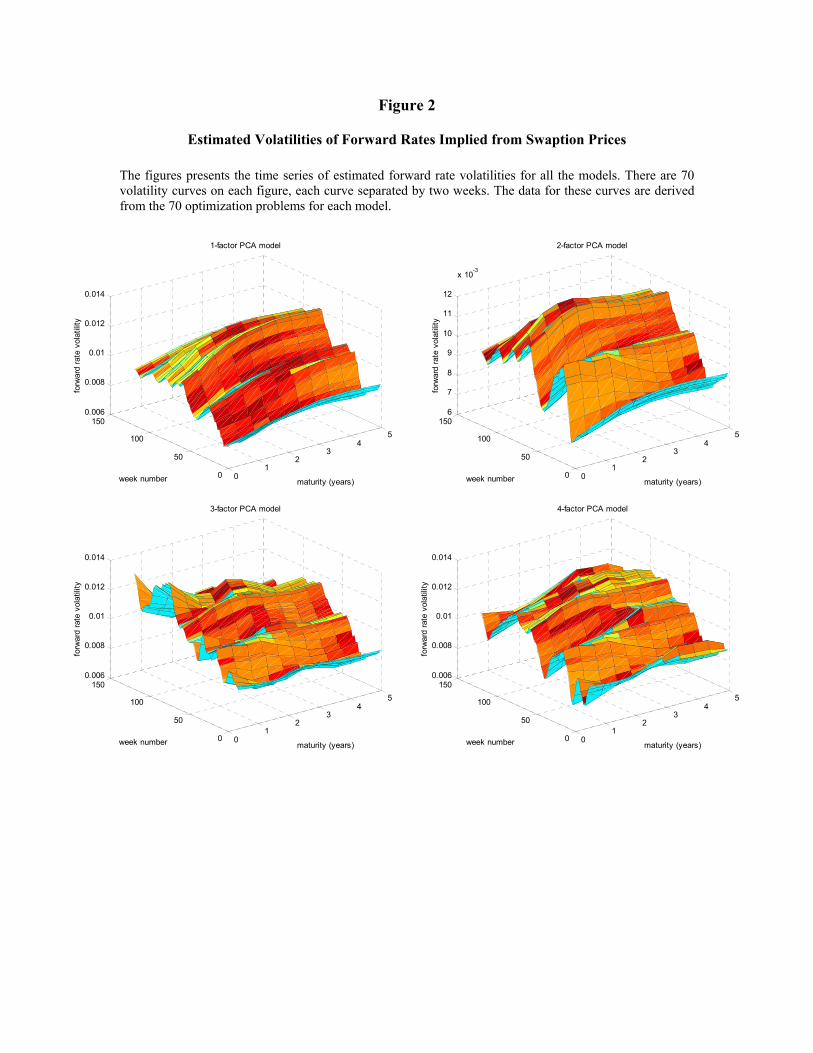
Figure 2

Estimated Volatilities of Forward Rates Implied from Swaption Prices

The figures presents the time series of estimated forward rate volatilities for all the models. There are 70 volatility curves on each figure, each curve separated by two weeks. The data for these curves are derived from the 70 optimization problems for each model.

01

23

45

0

50

100

1500.006

0.008

0.01

0.012

0.014

maturity (years)

1-factor PCA model

week number

forw

ard

rate

vol

atili

ty

01

23

45

0

50

100

1506

7

8

9

10

11

12

x 10-3

maturity (years)

2-factor PCA model

week number

forw

ard

rate

vol

atili

ty

01

23

45

0

50

100

1500.006

0.008

0.01

0.012

0.014

maturity (years)

3-factor PCA model

week number

forw

ard

rate

vol

atili

ty

01

23

45

0

50

100

1500.006

0.008

0.01

0.012

0.014

maturity (years)

4-factor PCA model

week number

forw

ard

rate

vol

atili

ty

Figure 3

Box and Whiskers Plots of Swaption Hedging Errors

This figure presents the box and whiskers plots for the one week hedging errors, for swaptions across all expirations and underlying swap maturities. The corresponding plots for the unhedged swaptions are presented for comparison purposes. In each figure, the first box corresponds to the unhedged swaption, the second box to the one-factor model, the third box to the two-factor model, the fourth box to the three-factor model, and the fifth box to the four-factor model.

Expiration = 0.5

Swap Maturity

5432

Basi

s Po

ints

20

0

-20

Expiration = 1

Swap Maturity

5432

Basi

s Po

ints

20

0

-20

Expiration = 2

Swap Maturity

5432

Basi

s Po

ints

20

0

-20

Expiration = 3

Swap Maturity

5432

Basi

s Po

ints

20

0

-20

Expiration = 4

Swap Maturity

5432

Basi

s Po

ints

20

0

-20

Expiration = 5

Swap Maturity

5432

Basi

s Po

ints

20

0

-20

Figure 4

Box and Whiskers Plots of Swaption Straddle Gamma Hedging Errors This figure presents the box and whiskers plots for the one week hedging errors, for swaption straddles across all expirations and underlying swap maturities. The corresponding plots for the unhedged straddles are presented for comparison purposes. In each figure, the first box corresponds to the unhedged swaption, the second box to the one-factor model, the third box to the two-factor model, the fourth box to the three-factor model, and the fifth box to the four-factor model.

Expiration = 0.5

Swap Maturity

5432

Basi

s Po

ints

15

0

-15

Expiration = 1

Swap Maturity

5432

Basi

s Po

ints

15

0

-15

Expiration = 2

Swap Maturity

5432

Basi

s Po

ints

15

0

-15

Expiration = 3

Swap Maturity

5432

Basi

s Po

ints

15

0

-15

Expiration = 4

Swap Maturity

5432

Basi

s Po

ints

15

0

-15

Expiration = 5

Swap Maturity

5432

Basi

s Po

ints

15

0

-15

Figure 5

Time Series of Swaption Straddle Hedging Errors Explained by the Four-Factor Model The figure compares the time series of the percentage of straddle hedging errors explained by the four-factor model, across all contracts by quarter, when the eigenvalues of the four-factor model are updated every second week, with the percentage from the same model with no parameter updating. In the figure, the lower line represents the percentage of the unhedged straddle error, as measured by the total sum of squared error for all contracts over the quarter, explained by the four-factor model with no recalibration. The upper line represents the corresponding percentage for the four-factor model when it is periodically recalibrated. Each percentage is based on 144 observations.

0%

20%

40%

60%

80%

100%

1 2 3 4 5 6 7 8 9 10 11 12

Quarter

Per

cent

age

Erro

r Exp

lain

ed

No Recalibration

With Recalibration