PRICING AND HEDGING OPTIONS UNDER

STOCHASTIC VOLATILITY

by

Jianqiang Xu

B.Sc., Peking University, China, 2003

AN ESSAY SUBMITTED IN PARTIAL FULFILLMENT OF

THE REQUIREMENTS FOR THE DEGREE OF

MSC MATHEMATICAL FINANCE

in

THE FACULTY OF GRADUATE STUDIES

(Department of Mathematics)

We accept this essay as conformingto the required standard

The University of British Columbia

March 2005

c© Jianqiang Xu, 2005

Abstract

In this essay, I mainly discuss how to price and hedge options in stochastic volatility(SV) models. The market is incomplete in the SV model, whereas it is completein the Black-Scholes model. Thus the option pricing and hedging methods are alittle different for the SV model and for the Black-Scholes model. The no-arbitrageargument and the risk-neutral valuation method are two general methods for pricingoptions. Both methods can be applied to the SV model. Heston’s SV model isdiscussed in more details, since it is the most popular SV model in practice. I alsoimplement Heston’s model and investigate the effects of the model parameters bylooking at the pricing results.

ii

Contents

Abstract ii

Contents iii

Acknowledgements iv

1 Introduction 1

2 Evidence of Stochastic Volatility 32.1 Black-Scholes Model and Volatility Smile . . . . . . . . . . . . . . . 32.2 Econometric Evidence . . . . . . . . . . . . . . . . . . . . . . . . . . 62.3 Some Approaches to Dealing with Volatility Smile . . . . . . . . . . 7

3 Stochastic Volatility Models 103.1 A General Model . . . . . . . . . . . . . . . . . . . . . . . . . . . . . 103.2 Pricing Options . . . . . . . . . . . . . . . . . . . . . . . . . . . . . . 113.3 Hedging Options . . . . . . . . . . . . . . . . . . . . . . . . . . . . . 15

4 A Special Case: Heston’s SV Model 184.1 An Introduction to the Model . . . . . . . . . . . . . . . . . . . . . . 184.2 A Closed-Form Solution . . . . . . . . . . . . . . . . . . . . . . . . . 194.3 Implementations and Results . . . . . . . . . . . . . . . . . . . . . . 224.4 Estimation of Parameters . . . . . . . . . . . . . . . . . . . . . . . . 25

5 Limitations of Stochastic Volatility Models 28

6 Conclusion 30

Bibliography 32

iii

Acknowledgements

I would like to thank my supervisor, Dr. Ivar Ekeland, for his helpful advice duringthe research and writing of this essay. I also wish to thank all my friends at UBCfor making my stay in Vancouver enjoyable. Finally special thanks to my parentsfor their support and encouragement.

Jianqiang Xu

The University of British ColumbiaMarch 2005

iv

Chapter 1

Introduction

In their seminal paper on option pricing, Black and Scholes (1973) presented afamous option pricing formula. They assume the stock price follows a geometricBrownian motion with a constant volatility. A riskless portfolio is formed by a calloption and some shares of stock. Based on no-arbitrage arguments, a partial differ-ential equation can be derived for the price of a call option. This partial differentialequation can be easily solved and gives a closed-form solution. Because of its sim-plicity and its independence of investors’ expectations about future asset returns,the Black-Scholes (B-S) formula is widely used among practitioners for pricing andhedging options. However, a number of studies have shown that the B-S model hassystematic biases across moneyness and maturity. The most well-known result ofthe B-S model is the so-called volatility smile or skew. The implied volatilities fromthe market prices of options tend to vary by strike prices and maturities. It is clearthat some assumptions of the B-S model are too strong. Empirical studies find stockreturns usually have a higher kurtosis compared to the normal distribution which isassumed by the B-S model. Some people also model stock volatilities as a stochasticprocess, either discrete or continuous.

In order to reduce the option pricing error, researchers have presented sev-eral approaches. Many traders prefer to remain in the B-S framework and simplyuse the volatility matrix or a fitted volatility function and then apply the B-S for-mula in a modified way. Other one-factor models include the constant elasticityof variance (CEV) model (Cox and Ross (1976)), and the local volatility models(Derman and Kani (1994), etc.). The market is complete in one-factor models.Some models are extended to have multiple factors. This group includes the jump-diffusion model (Merton (1976)), the continuous-time stochastic volatility model(Hull and White (1987), Stein and Stein (1991), Heston (1993)), and the GARCHoption pricing model (Duan (1995), Heston and Nandi (2000)). Other models arehybrids, combining some aspects of standard models. Bates (1996)’s stochastic

1

volatility/jump-diffusion model is a good example.In this essay, I will discuss how to price and hedge options in the SV model.

In finance literature, several methods are employed to price options. We can form ariskless portfolio and apply no-arbitrage arguments to give an option price based onthe underlying stock price. We can also find an equivalent martingale measure andapply risk-neutral valuation methods. Both methods can be used in the SV modelas well as in the B-S model. But the application procedures are different as themarket is complete in the B-S model but incomplete in the SV model. Some peoplealso apply utility functions to pricing options. But in practice, pricing methodsbased on utility functions are very difficult to implement.

In the B-S model, a perfect hedging is possible due to the market complete-ness. However, in SV models, the market is incomplete and a perfect hedging isimpossible. Practitioners can either use other options to hedge the target option,or only use the underlying stock to partially hedge the option. Popular hedgingstrategies for SV models in finance literature include superhedging, mean-variancehedging and shortfall hedging.

The rest of the essay is organized as follows. Chapter 2 introduces the optionpricing methods and the results in the B-S model. This serves to give a comparisonwith the results in the SV model. The pricing biases in the B-S model and theeconometric evidence of stochastic volatility will be discussed. I will also give a verybrief introduction to some popular models in option pricing literature. Chapter 3discusses pricing and hedging options in SV models. Chapter 4 takes Heston’s SVmodel as an example to discuss some implementation issues. The implied volatilitysurface in Heston’s model is plotted. Effects of some model parameters are inves-tigated. I will also present some parameter estimation methods for SV models.Chapter 5 discusses some limitations of SV models. Chapter 6 concludes this essay.

2

Chapter 2

Evidence of Stochastic Volatility

2.1 Black-Scholes Model and Volatility Smile

In the B-S world, the stock price, S, follows a geometric Brownian motion,

dSt = µStdt + σStdz, (2.1)

where µ and σ are known constants, z is a standard Brownian motion. To derive theoption pricing formula, Black and Scholes (1973) make some other assumptions, suchas the market is frictionless, the short-term interest rate is known and a constant,r, short selling is allowed without restrictions, the stock pays no dividends. Theessential step in the B-S methodology is the construction of a riskless portfolio andthe no-arbitrage argument. The main derivation goes as follows.

Suppose that f is the price of a call option or other derivative contingent onS. By Ito’s lemma,

df = (∂f

∂SµS +

∂f

∂t+

12

∂2f

∂S2σ2S2)dt +

∂f

∂SσSdz. (2.2)

Next, we set up a portfolio consisting of a short position in a call option and a longposition of ∆ units of stock. Define Π as the value of the portfolio,

Π = −f + ∆S. (2.3)

The change in the value of this portfolio in a small time interval is given by

dΠ = −df + ∆dS. (2.4)

Substituting (2.1), (2.2) into (2.4) yields

dΠ = −(∂f

∂SµS +

∂f

∂t+

12

∂2f

∂S2σ2S2)dt− ∂f

∂SσSdz + ∆µSdt + ∆σSdz

= (−∂f

∂SµS − ∂f

∂t− 1

2∂2f

∂S2σ2S2 + ∆µS)dt + (−∂f

∂SσS + ∆σS)dz. (2.5)

3

To make the portfolio riskless, we choose ∆ = ∂f∂S . Then,

dΠ = (−∂f

∂t− 1

2∂2f

∂S2σ2S2)dt. (2.6)

On the other hand, in the absence of arbitrage opportunities, this riskless portfoliomust earn a risk-free rate, r,

dΠ = rΠdt. (2.7)

Substituting from (2.3) and (2.6), this becomes

(−∂f

∂t− 1

2∂2f

∂S2σ2S2)dt = r(−f +

∂f

∂SS)dt,

or

∂f

∂t+ rS

∂f

∂S+

12σ2S2 ∂2f

∂S2= rf. (2.8)

Equation (2.8) is the famous B-S partial differential equation. The solutiondepends on the boundary conditions. In the case of a European vanilla call option,the final condition is that the option price is simply its payoff at maturity.

f = max(S −K, 0), t = T, (2.9)

where K is the strike price. So the equation can be solved by backward in time withthe final condition. The B-S pricing formula for the European call option is

c = S0N(d1)−Ke−rT N(d2), (2.10)

where

d1 =ln(S0/K) + (r + σ2/2)T

σ√

T, d2 =

ln(S0/K) + (r − σ2/2)Tσ√

T= d1−σ

√T , (2.11)

and S0 is the current stock price, T is the time to maturity, σ is the stock pricevolatility, N(x) is the cumulative probability distribution function for the standardnormal distribution. The price of the European put option can be computed by theput-call parity.

The expected return µ does not appear in the B-S equation. This meansthe pricing formula is independent of the individual’s preference. This amazingproperty together with its simplicity makes the B-S pricing formula very popularamong practitioners as well as academic researchers.

4

Another approach to deriving the B-S formula is the risk-neutral valuationmethod. The price of the option, c, is the expected value of the option at maturityin a risk-neutral world discounted at the risk-free interest rate, that is

c = e−rT EQ[max(ST −K, 0)], (2.12)

where EQ denotes the expected value in a risk-neutral world. Q is also called theequivalent martingale measure. In the risk-neutral world, ST = S0e

(r−σ2/2)T+σz. Sothe expectation in (2.12) can be calculated by integrating over the normal distribu-tion. We can get the same pricing formulas as (2.10) and (2.11). The above twopricing methods, no-arbitrage valuation and risk-neutral valuation, are two generalapproaches to pricing options in modern finance literature.

Although the B-S formula is powerful to price stock options and simple touse, many empirical results show that it may systematically misprice a number ofoptions. The well-known phenomenon related to the biases of the B-S model is thevolatility smile or skew.

The implied volatility is the volatility used in the B-S model such that theobserved market price of the option equals the model price.

cBS(σ) = cMarket. (2.13)

Consider call or put options on a given stock or an index. These options havethe same maturity but different strike prices. We apply the B-S model to backout the implied volatilities and plot them against the strike prices. We expect theimplied volatilities to be identical because the constant volatility is the assumptionof the B-S model. However, it is likely not the case in practice. Most optionmarkets exhibit persistent patterns of non-constant volatilities. In some markets,the implied volatilities form a ‘U-shape’, which is called the volatility smile. In-the-money options and out-of-the-money options have higher implied volatilities thanat-the-money options. Generally, the shape of the volatility smile is not symmetric.It is more of a skewed curve. People also call it volatility skew or volatility smirk.Figure 2.1 is the implied volatilities of S&P 500 European call options at variousstrike prices on Feb. 24, 2005. All these options mature on Jun. 17. Obviously, thephenomenon of volatility smile is not consistent with the B-S model.

In addition to calculating a volatility smile, we can also calculate a volatilityterm structure, a function of maturity for a fixed strike price. The implied volatilitiesalso vary with maturity. Combining the volatility smile and the volatility termstructure, we can generate a volatility surface, one dimension for strike price andthe other for maturity. Usually, the smile is significant for short maturity optionsand tends to be flat for long maturity options.

5

950 1000 1050 1100 1150 1200 1250 1300 13500.08

0.1

0.12

0.14

0.16

0.18

0.2Volatility Smile for S&P 500 Call Options

Strike Price

Impl

ied

Vola

tility

Figure 2.1: Implied volatilities for S&P 500 call options. Maturity is Jun. 17, 2005.Valuation date is Feb. 24, 2005. The S&P 500 index is 1200.20 on the valuationday. Use r = 0.011.

There are various explanations for the phenomenon of volatility smile. Someof explanations are related to the idealized assumption of the B-S model which saysthe asset price follows a geometric Brownian motion with a constant volatility. Iprovide some econometric evidence against this assumption of the B-S model.

2.2 Econometric Evidence

If the stock price follows a geometric Brownian motion as in equation (2.1), the stockprice is lognormally distributed, or, the logarithmic return is normally distributed.From Figure 2.2, we see that price changes are small in sequential days in someperiods and large in other periods. This is called volatility clustering. This featureimplies that the volatility is autocorrelated.

People also find that the return distribution has leptokurtosis, which hashigher central peak and fatter tails compared with the normal distribution. Lep-tokurtosis is consistent with the volatility smile. It is usually a result of a mixtureof several distributions with different variances.

Based on the above facts, people have tried to model the volatilities. Ineconometrics, ARCH-type models are very popular to model volatilities. An ARCH(Autoregressive conditional heteroskedasticity) process can be defined in the follow-ing way. Assume the dependent variable yt is generated by

yt = x′tζ + εt, t = 1, 2...T, (2.14)

6

0 200 400 600 800 1000 1200−0.08

−0.06

−0.04

−0.02

0

0.02

0.04

0.06S&P 500 Returns 2000−2004

Time

Inde

x Le

vel

Figure 2.2: S&P 500 daily returns from Jan. 3, 2000 to Dec. 31, 2004

where xt is a vector of exogenous variables, which may include lagged dependentvariable, and ζ is a vector of regression parameters. Engle (1982) characterizes thestochastic error ε as an ARCH process,

εt|φt−1 ∼ N(0, ht), (2.15)

ht = α0 + α1ε2t−1 + ... + αqε

2t−q, (2.16)

with α0 > 0, and αi ≥ 0, i = 1, ..., q, to ensure that the conditional variance ispositive. Bollerslev (1986) proposes a GARCH (Generalized ARCH) model. Theconditional variance in GARCH models is specified as

ht = α0 + α1ε2t−1 + ... + αqε

2t−q + β1ht−1 + ... + βpht−p, (2.17)

with α0 > 0, αi ≥ 0, i = 1, ..., q, and βj ≥ 0, j = 1, ..., p. A GARCH process withorders p and q is denoted as GARCH(p,q). There are several other versions ofGARCH models, such as exponential GARCH, GJR GARCH, non-linear GARCH,etc. GARCH models are the most successful models to model the volatilities offinancial time series. They have been applied in several finance fields.

2.3 Some Approaches to Dealing with Volatility Smile

Practitioners and researchers have proposed many methods to deal with the problemof volatility smile. The simplest way to incorporate the volatility smile is to use thevolatility matrix. Market prices of options are used to generate implied volatilities.The volatility matrix replicates the volatility surface. When we want to price a new

7

option, we can pick up a corresponding volatility and apply the B-S model to getthe price. An alternative way to account for the volatility smile is to smooth theimplied volatility relation across strike prices and maturities. For example, Dumas,Fleming and Whaley (1998) use the following function to fit the volatility surface,

σ = a0 + a1K + a2K2 + a3T + a4T

2 + a5KT, (2.18)

where K is the strike price and T is the time to maturity. Applying the B-S modelin this way is internally inconsistent because the B-S model assumes a constantvolatility. But this procedure is quite useful in practice as a means of predictingoption prices. Many empirical researchers employ this ad hoc Black-Scholes modelwhen they test other complicated models. In many cases, this simple model is foundto be able to beat those complicated models.

One way to modify the constant volatility assumption of the B-S model is toassume that volatility is a deterministic function of time and stock price: σ = σ(t, S).In the special case of σ = σ(t), a deterministic function of time, the option pricewill just be the B-S formula with volatility

√σ2, where σ2 = 1

T

∫ T0 σ2(s)ds.

Another famous model with deterministic volatility is the constant elasticityof variance (CEV) model proposed by Cox and Ross (1976). The stock price in thismodel is

dS = µSdt + σSαdz, (2.19)

where α is a positive constant. So the stock price has volatility σSα−1. When α = 1,we have the Black-Scholes case. When α < 1, the volatility increases as the stockprice decreases. This can generate a distribution with a fatter left tail and a thinnerright tail. When α > 1, the situation is reversed. So the volatility smile can beincorporated in this model. Cox and Ross (1976) also provide valuation formulasfor European call and put options in the CEV model. Several studies have reportedthat the CEV model outperforms the B-S model in most cases. The problem of themodel is that the option price in the CEV model will approach either zero or infinitein the long run.

Derman and Kani (1994) proposed a so-called implied tree model, which alsoassumes that the volatility is a deterministic function of stock price and time. Theimplied tree model is also called the local volatility model. The model has severalversions developed by different researchers. These models incorporate the volatilitysmile in the construction of the tree. And this tree is particularly used for pricingexotic options. By the implied tree, the prices of exotics are consistent with alltraded vanilla options. Implied trees are quite heavily used among traders. But itis difficult to get them to calibrate vanilla market data, because the local volatilitysurface can be very irregular.

8

Deterministic volatility models allow volatility to change in a deterministicway. But empirical evidence shows the variance of the stock returns is not station-ary. The relation between the volatility and the stock or time changes with time.We model the volatility as a function of the stock price and time this week. Butnext week, this function will be quite different. Hence, it is not enough to allowvolatility to change deterministically. Subsequent researches model the volatility asa stochastic variable. In SV models, volatility is modelled as a separate stochasticprocess. Details about SV models will be discussed in Chapter 3.

Another important strand in option pricing models is modelling stock priceswith jumps. These models are motivated by the fact that the price exhibits jumpsrather than continuous changes. Merton (1976) added random jumps to the geo-metric Brownian motion. The stochastic process for the stock price is

dS

S= (µ− λk)dt + σdz + dp, (2.20)

where λ is an average number of jumps per year, k is the average jump size, dp isthe Poisson process generating the jumps, other parameters are similar to those inthe B-S model. This jump diffusion model is useful when the underlying asset pricehas large changes, because continuous-time models cannot capture this property.

Some other researchers even model the stock price as a pure jump process.They also combine stochastic volatility and jump diffusion. Stock prices in thesecomplicated models can have many good properties. But these models are hard toimplement.

In this essay, I focus on SV models and take Heston’s SV model as an exampleto discuss the implementation. The SV model has become more and more popularamong practitioners and academic researchers. It is said to be the next generationof the option pricing model. Heston’s SV model is easy to implement. This makesHeston’s SV model the most popular SV model.

9

Chapter 3

Stochastic Volatility Models

3.1 A General Model

A general representation of the continuous-time SV model we are considering maybe written as

dSt = µStdt + σtStdW1t, (3.1)

σt = f(Yt), (3.2)

dYt = a(t, Yt)dt + b(t, Yt)dZt, (3.3)

dW1tdZt = ρdt. (3.4)

Here the drift µ is still a constant. σt is the volatility of the stock price.f is some positive function. Yt is some underlying process which determines thevolatility. W1t and Zt are two correlated standard Brownian motions. The constantparameter ρ is the correlation coefficient between these two Brownian motions. Wecan also rewrite Zt as

Zt = ρW1t +√

1− ρ2W2t, (3.5)

where W2t is a standard Brownian motion independent of W1t. There are someeconomic arguments for a negative correlation between stock price and volatilityshocks. Empirical studies also show ρ < 0 from stock data.

This general SV model contains many famous SV models in financial litera-ture. The following are three examples.

(1) Hull-White Hull and White (1987) assume a geometric Brownian motion forthe variance,

dYt = αYtdt + βYtdZt, (3.6)

10

where α and β are constants. f(y) =√

y. This is the first SV model for pricingoptions in financial literature. Hull and White derived a closed-form formula forthe European option in a particular case in which ρ = 0. Generally, numericaltechniques are required when implementing this model.

(2) Stein-Stein Stein and Stein (1991) assume the driving process Yt is an Ornstein-Uhlenbeck (OU) process,

dYt = α(ω − Yt)dt + βdZt. (3.7)

It is a mean-reverting process. From econometric studies, people believe that volatil-ity is mean-reverting. So OU process is employed by many researchers to model thevolatility. But it is not appropriate to simply assume that the volatility is an OUprocess, because Yt can be negative in OU process. Stein and Stein (1991) assumef(y) = |y|. They also give a closed-form formula for the European option whenρ = 0. Some other people use f(y) = ey instead, e.g. Scott (1987).

(3) Heston Heston (1993) assumes Yt follows a Cox-Ingersoll-Ross (CIR) pross,

dYt = κ(θ − Yt)dt + ξ√

YtdZt, (3.8)

and f(y) =√

y. Yt is strictly positive when 2κθ ≥ ξ2 and non-negative when0 ≤ 2κθ < ξ2. This model is very important because it provides a closed-formformula for the European option and ρ can be non-zero. It will be discussed indetails in the next section.

3.2 Pricing Options

In order to price options in the SV model, we can apply no-arbitrage arguments, oruse the risk-neutral valuation method. First we discuss the no-arbitrage method.The riskless portfolio is constructed as in the Black-Scholes model. But the construc-tion method is different. In the SV option pricing model, there is only one tradedrisky asset S but two random sources W1t and Zt. So the market is incomplete. Wecannot perfectly replicate the option solely with the underlying stock. No-arbitragearguments are not enough to give the option price. We need additional assumptions.In the following derivation, equilibrium arguments are also employed. We know thatthe market can be completed by adding any option written on stock S. Simply, themarket is complete when we have two traded assets, the underlying asset S and abenchmark option G. Then all other options can be replicated by these two traded

11

assets. A riskless portfolio Π consists of an option F which we want to price, −∆1

shares of the underlying asset S, and −∆2 shares of the benchmark option G.

Π = F −∆1S −∆2G. (3.9)

The portfolio is self-financing, so that

dΠ = dF −∆1dS −∆2dG. (3.10)

F and G are functions of variables t, St and Yt. By applying the two-dimensional vertion of Ito’s formula, (3.10) becomes

dΠ =[∂F

∂t+

12f(Y )2S2 ∂2F

∂S2+

12b2 ∂2F

∂Y 2+ ρf(Y )Sb

∂2F

∂S∂Y

]dt +

∂F

∂SdS +

∂F

∂YdY

−∆1dS −∆2

{[∂G

∂t+

12f(Y )2S2 ∂2G

∂S2+

12b2 ∂2G

∂Y 2+ ρf(Y )Sb

∂2G

∂S∂Y

]dt

+∂G

∂SdS +

∂G

∂YdY

}. (3.11)

We can rewrite it by collecting the terms of dt, dS and dY,

dΠ =[∂F

∂t+

12f(Y )2S2 ∂2F

∂S2+

12b2 ∂2F

∂Y 2+ ρf(Y )Sb

∂2F

∂S∂Y

]dt

−∆2

[∂G

∂t+

12f(Y )2S2 ∂2G

∂S2+

12b2 ∂2G

∂Y 2+ ρf(Y )Sb

∂2G

∂S∂Y

]dt

+[∂F

∂S−∆2

∂G

∂S−∆1

]dS +

[∂F

∂Y−∆2

∂G

∂Y

]dY. (3.12)

To make the portfolio riskless, we choose

∂F

∂S−∆2

∂G

∂S−∆1 = 0, (3.13)

∂F

∂Y−∆2

∂G

∂Y= 0 (3.14)

to eliminate dS term and dY term. Solving (3.13) and (3.14) gives

∆2 =∂F

∂Y

/∂G

∂Y, (3.15)

∆1 =∂F

∂S− ∂G

∂S

∂F

∂Y

/∂G

∂Y(3.16)

12

The portfolio is riskless if we rebalance it according to (3.15) and (3.16). On theother hand, the riskless portfolio must earn a risk-free rate, otherwise there wouldbe an arbitrage opportunity. So

dΠ =[∂F

∂t+

12f(Y )2S2 ∂2F

∂S2+

12b2 ∂2F

∂Y 2+ ρf(Y )Sb

∂2F

∂S∂Y

]dt

−∆2

[∂G

∂t+

12f(Y )2S2 ∂2G

∂S2+

12b2 ∂2G

∂Y 2+ ρf(Y )Sb

∂2G

∂S∂Y

]dt

= rΠdt, (3.17)

where Π is given by (3.9). Substituting (3.15) and (3.16) into (3.17) gives[∂F

∂t+

12f(Y )2S2 ∂2F

∂S2+

12b2 ∂2F

∂Y 2+ ρf(Y )Sb

∂2F

∂S∂Y− rF + rS

∂F

∂S

]/∂F

∂Y

=[∂G

∂t+

12f(Y )2S2 ∂2G

∂S2+

12b2 ∂2F

∂Y 2+ ρf(Y )Sb

∂2G

∂S∂Y− rG + rS

∂G

∂S

]/∂G

∂Y.(3.18)

Notice that the left-hand side is a function of F only and the right-hand side is afunction of G only. The only way that this equation holds is that both sides areequal to some function, −k(t, S, Y ), which is independent of any particular option.The equation for the option F can be written as

∂F

∂t+

12f(Y )2S2 ∂2F

∂S2+

12b2 ∂2F

∂Y 2+ρf(Y )Sb

∂2F

∂S∂Y−rF +rS

∂F

∂S= −k(t, S, Y )

∂F

∂Y.

(3.19)

We denote k(t, S, Y ) by

k(t, S, Y ) = a(t, Y )− b(t, Y )Λ(t, S, Y ), (3.20)

where a(t, Y ) is the drift term of the driving process Yt, Λ(t, S, Y ) is called themarket price of volatility risk. Λ(t, S, Y ) can not be determined by the arbitragetheory alone. In theory, it is completely determined by the benchmark option G. Sothe market determines the price of volatility risk. Finally, the PDE for the optionbecomes

∂F

∂t+

12f(Y )2S2 ∂2F

∂S2+

12b2 ∂2F

∂Y 2+ρf(Y )Sb

∂2F

∂S∂Y−rF +rS

∂F

∂S+(a−bΛ)

∂F

∂Y= 0.

(3.21)

Given the terminal condition for F, the PDE (3.21) is solvable under some specialdriving processes.

We can also apply the risk-neutral valuation method to the SV model. Themarket is incomplete. But it is still free of arbitrage. The equivalent martingale

13

measure is not unique. We have to choose one of all these measures to price theoptions. So the price of the option is also not unique. It will depend on whichequivalent martingale measure we use.

The problem here is how to construct equivalent martingale measures andwhat the asset price process and the volatility process will be under these mea-sures. To change measure from the objective measure P to an equivalent mar-tingale measure Q, we need to use the Girsanov Theorem. Recall that we havetwo Brownian motions in the SV model, W1t and Zt. And Zt can be expressed asZt = ρW1t +

√1− ρ2W2t, where W1t and W2t are independent. Under any equiv-

alent martingale measure Q, the underlying stock St will have a drift rSt. Thenthe discounted stock price will be a martingale under Q. But it is not the case forvolatility σt or the underlying driving process Yt, because volatility is not a tradedasset.

To make the the drift term of the stock price process be rSt under Q, we set

dW̃1t = dW1t +µ− r

f(Yt)dt. (3.22)

Since W2t is independent of W1t, shift of W2t will not change the drift of the stockprice process. We choose the shift of W2t as

dW̃2t = dW2t + γtdt. (3.23)

By the Girsanov Theorem, W̃1t and W̃2t are two independent standard Browmianmotions under the measure Q, which is defined by the following Radon-Nikodymderivative

dQ

dP= exp

(−1

2

∫ T

0(θ2

1t + θ22t)dt−

∫ T

0θ1tdW1t −

∫ T

0θ2tdW2t

), (3.24)

where

θ1t =µ− r

f(Yt),

θ2t = γt.

Here γt is an adapted process. To make Q be a probability measure, we need tomake some assumptions on f and γt. Under the measure Q

dSt = rStdt + σtStdW̃1t, (3.25)

σt = f(Yt), (3.26)

dYt = [a(t, Yt)− b(t, Yt)Λ(t, St, Yt)]dt + b(t, Yt)dZ̃t, (3.27)

14

where

Z̃t = ρW̃1t +√

1− ρ2W̃2t, (3.28)

Λ(t, St, Yt) = ρθ1t +√

1− ρ2θ2t = ρµ− r

f(Yt)+

√1− ρ2γt. (3.29)

For every choice of regular enough process γt, we get an equivalent martingalemeasure Q which we can use it to price options. Let Vt be the price of an optionwith payoff H at maturity T, then the price of the option is

Vt = EQ[e−r(T−t)H|Ft]. (3.30)

When γ = γ(t, St, Yt), we have the Markovian setting. Applying Feynman-Kac theorem, we can get the same partial differential equation as (3.21). In practice,we can also use the Monte Carlo simulation to evaluate (3.30).

Λ(t, St, Yt) in equation (3.21) is the same as that in (3.27), although thederivation is independent. Recall that Λ(t, St, Yt) is called the market price ofvolatility risk. This name is very natural when we look at the drift term of theprocess dYt in (3.27). Notice that in equation (3.21), the coefficient of ∂F

∂Y is just therisk-neutralized drift term of the process dYt, which is a(t, Yt) − b(t, Yt)Λ(t, St, Yt).While the coefficient of ∂F

∂S is also the risk-neutralized drift term rS. So now weknow why we choose k(t, S, Y ) to have the form (3.20). Further more, we know from(3.29) that Λ(t, St, Yt) can be decomposed into two parts which correspond to thetwo independent Brownian motion.

3.3 Hedging Options

In this section, I will give a brief introduction to some hedging strategies understochastic volatility. In the B-S world, the market is complete. An option canbe perfectly hedged by dynamically trading the underlying stock. The delta ofan option, ∆, was introduced in Section 2.1 when deriving the B-S equation. Aportfolio consisting of a short position in a call option and ∆ units of stocks islocally riskless. Generally, the delta can be defined as the rate of change of optionprice F with respect to the stock price S,

∆ =∂F

∂S. (3.31)

However, the market is incomplete in the SV model. A perfect hedging is impossibleby trading only the underlying stock. In the following several paragraphs, I introducesome option hedging strategies for the SV model.

15

We know from Section 3.2 that the market can be completed by adding abenchmark option G. So a perfect hedging can be achieved by trading the option Gas well as the underlying stock S. Suppose that we want to hedge a short positionin a call option F with strike price K. Option G can be a call option with the samematurity but a different strike price K ′ . From Section 3.2, the hedger will need aposition in (i) ∆1 units of the underlying stock, and (ii) ∆2 units of option G, where∆1 and ∆2 are given by (3.15) and (3.16). Traders define the vega of a portfolio(or an option) as the rate of change of the value of the portfolio with respect to thevolatility of the underlying stock,

ν =∂F

∂σ. (3.32)

So the vega represents the volatility risk of the option. The hedging strategy wediscussed above is similar to the construction of a delta-neutral and also vega-neutralportfolio.

We know now by dynamically trading the underlying asset and another op-tion, both the price risk and the volatility risk can be hedged. In practice, continuoustrading is impossible. Traders can rebalance the portfolio daily or at other frequen-cies. If the frequency is high, the transaction cost can be a problem. The transactioncost is much higher for trading options than for trading stocks. So traders preferto use stocks to hedge options. Researchers have proposed some hedging strategiesusing only stocks in incomplete markets. Superhedging, mean-variance hedging andshortfall hedging are three frequently discussed strategies in financial literature.

Consider a path-independent claim with a payoff H(ST ) at maturity T. If thepayoff H(ST ) is affine in the stock, then this claim can be perfectly replicated evenif in the incomplete market. However, most claims are not affine in the stock, e.g.European call options. A superhedging is a trading strategy π, which starts withan initial wealth x, and has a terminal payoff Xx,π(T ) ≥ H(ST ) almost surely. Asimple example of superhedging is to buy one unit of stock to hedge a short positionin a call option. The task here is to find the cheapest superhedging, which is anupper bound of the option price,

P up = inf{x ≥ 0, ∃π, Xx,π(T ) ≥ H(ST )}. (3.33)

Cvitanic, Pham, and Touzi (1999) analyze superheding for the SV model. From theviewpoint of the option writer, the superhedging is very attractive, since his hedgingportfolio always has a value no less than the written option. But in practice, thesuperhedging solution for the SV model is not very satisfactory. An investor cannotcharge P up when he enters a short position in an option contract. Usually the initialcost P up for a superhedging strategy is unfeasibly high in the SV model. In realistic

16

situations, the option premium is lower than P up. So the investor with a shortposition cannot implement a superhedging strategy. So he is unable to eliminateall the risk. Therefore he has to find a more realistic hedging strategy under a costconstraint which is the option premium.

Follmer and Sondermann (1986) use a quadratic loss function to assess thequality of trading strategies. Since a perfect replication is impossible in incompletemarkets, they instead try to partially hedge the risk as much as possible, i.e. to finda trading strategy that most closely approximate the payoff under some criteria.One natural criteria is minimizing the mean-squared error. Following the previousdenotation, the optimal replication problem becomes,

minπ

E[Xx,π(T )−H(ST )]2. (3.34)

This leads to the notion of mean-variance hedging.Another choice of the criteria is

minπ

E[l((Xx,π(T )−H(ST ))+)] (3.35)

where l is a convex function corresponding to risk aversion. The simple quadraticloss function is replaced by a loss function representing a shortfall risk. The problemof using a quadratic loss function is both the shortfalls and overshoots are penalized.But in practice the overshoot should not receive a penalty. In (3.35) only the shortfallis penalized. The shortfall risk is defined as the expectation of the shortfall weightedby the loss function l. Interested readers can find the results of the shortfall hedgingstrategy in Follmer and Leukert (2000).

17

Chapter 4

A Special Case: Heston’s SV

Model

4.1 An Introduction to the Model

SV models have been used by many traders to price and hedge options. Amongthe several existed SV models, Heston’s SV model is the most popular one. Thischapter will focus on Heston’s SV model. I will first introduce Heston’s setting forthe volatility process. The partial differential equation for the option price underHeston’s model will be provided. Then we will discuss how to solve this PDE for aEuropean option by a method based on characteristic functions. Greeks will also bederived. And then we will discuss the implementation of Heston’s model and someproperties of the model results.

Heston (1993) assumes Yt in (3.3) follows a Cox-Ingersoll-Ross (CIR) pross,

dYt = κ(θ − Yt)dt + ξ√

YtdZt, (4.1)

and f(y) =√

y. We rewrite the model in the following way for convenience,

dSt = µStdt +√

vtStdZ1t, (4.2)

dvt = κ(θ − vt)dt + ξ√

vtdZ2t, (4.3)

dZ1tdZ2t = ρdt, (4.4)

where Z1t and Z2t are two standard Brownian motions with correlation ρ. θ is thelong-run variance, κ is the rate of mean reversion, ξ is called volatility of volatilityor volatility of variance. Here we assume there is no dividend payment and theinterest rate is constant. By the same argument of Section 3.2, the value of any

18

option U(S, v, t) must satisfy the same PDE (3.21),

∂U

∂t+

12vS2 ∂2U

∂S2+

12ξ2v

∂2U

∂v2+ρξvS

∂2U

∂S∂v−rU+rS

∂U

∂S+{κ[θ−v]−Λ(S, v, t)ξ

√v}∂U

∂v= 0.

(4.5)

Λ(S, v, t) is the market price of volatility risk1. Heston (1993) chooses the marketprice of volatility risk to be proportional to the volatility, i.e. Λ(S, v, t) = k

√v.

Or Λ(S, v, t)ξ√

v = kξv. Let λ = kξ, so the coefficient of ∂U∂v in (4.5) becomes

{κ[θ − v] − λv}. This choice of market price of volatility risk gives us analyticaladvantages. The drift term of the specified process (4.3) is an affine function of thestate variable itself. The affinity makes the model easier to solve. The market priceof volatility risk is assigned to be proportional to the square root of the variance.Since the diffusion of the variance process is also proportional to the square root ofthe variance, the product of the market price of risk and the diffusion is proportionalto variance itself. As a result, the drift term will remain affine under the equivalentmartingale measure. This particular market price of volatility risk helps the modelto have a closed-form solution.

4.2 A Closed-Form Solution

Heston (1993) solves this equation for a European option by using a techniquebased on characteristic functions. This method can also be used to solve some otherimportant models, so we give a brief introduction here. The solution of the equationhas the form which is similar to the Black-Scholes formula,

C(S, v, t) = SP1 −Ke−r(T−t)P2. (4.6)

Let

x = ln(S), (4.7)

and substitute the proposed solution (4.6) into the (4.5). Then we have two PDEswhich P1 and P2 should satisfy,

12v∂2Pj

∂x2+ρξv

∂2Pj

∂x∂v+

12ξ2v

∂2Pj

∂v2+(r+ujv)

∂Pj

∂x+(a− bjv)

∂Pj

∂v+

∂Pj

∂t= 0, (4.8)

1In Heston (1993), the coefficient of ∂U∂v in (4.5) is {κ[θ− v]−Λ(S, v, t)}. The difference

comes from the different definition of Λ(S, v, t). Our definition is consistent with the notationin Section 3.2. The results will become the same after we specify Λ(S, v, t).

19

for j = 1, 2, where

u1 =12, u2 = −1

2, a = κθ, b1 = κ + λ− ρξ, b2 = k + λ. (4.9)

These PDEs must be solved subject to the terminal condition

Pj(x, v, T ; ln(K)) = 1{x≥ln(K)}. (4.10)

They can be interpreted as “risk-neutralized” probabilities. The corresponding char-acteristic functions f1(x, v, t;φ) and f2(x, v, t; φ) will satisfy similar PDEs,

12v∂2fj

∂x2+ρξv

∂2fj

∂x∂v+

12ξ2v

∂2fj

∂v2+(r +ujv)

∂fj

∂x+(a− bjv)

∂fj

∂v+

∂fj

∂t= 0 (4.11)

with the terminal condition

fj(x, v, T ; φ) = eiφx. (4.12)

Due to the linearity of the coefficients we guess a functional form

fj(x, v, t; φ) = eC(T−t;φ)+D(T−t,φ)v+iφx. (4.13)

Substituting this functional form into the PDE (4.11), we have two ordinary differ-ential equations,

−12φ2 + ρξφiD +

12ξ2D2 + ujφi− bjD +

∂D

∂t= 0, (4.14)

rφi + aD +∂C

∂t= 0, (4.15)

subject to the terminal condition C(0;φ) = 0, D(0;φ) = 0. 2 The solutions to thesetwo ODEs are

C(τ ; φ) = rφiτ +a

ξ2

{(bj − ρξφi + d)τ − 2ln

[1− gedτ

1− g

]}, (4.16)

D(τ ; φ) =bj − ρξφi + d

ξ2

[1− edτ

1− gedτ,

](4.17)

and

g =bj − ρξφi + d

bj − ρξφi− d, (4.18)

2The ODE(4.14) is a little different from the one in Heston 1993). I think there are sometypos in that paper.

20

d =√

(ρξφi− bj)2 − ξ2(2ujφi− φ2). (4.19)

Then the risk-neutral probabilities, P1 and P2 can be recovered by inverting thecorresponding characteristic functions,

Pj(x, v, t; ln(K)) =12

+1π

∫ ∞

0Re

[e−iφln(K)fj(x, v, t; φ)

iφ

]dφ. (4.20)

So the price of European call options is given by equations (4.6), (4.13), and(4.20). The price of European put options can be derived by the put-call parity.The essence of the characteristic function methodology is using Fourier analysis. Thegeneral inverse Fourier transform for pricing options is discussed in Lewis (2000).Fast Fourier transform algorithm is introduced by Carr and Madan (1999) to priceoptions.

Heston (1993) also incorporates the stochastic interest rates into the modeland apply the SV model to bond options and foreign currency options.

Since we have known the closed-form solution of the European call option,we can calculate the Greeks easily. Here I give the expressions of the three mostfrequently used Greeks: delta, gamma and vega.

The delta of the call is simply given by

∆ =∂C(S, v, t)

∂S= P1. (4.21)

The gamma of an option is defined as the second derivative of the option price withrespect to the stock price. So in Heston’s model, gamma is given by

Γ =∂2C(S, v, t)

∂S2=

∂∆∂S

=∂∆∂x

∂x

∂S=

1S

∂P1

∂x, (4.22)

and∂P1

∂x=

1π

∫ ∞

0Re[e−iφln(K)fj(x, v, t; φ)]dφ. (4.23)

Usually the vega of an option refers to the first derivative of the option with respectto volatility. For convenience, in Heston’s model we define vega as the first derivativewith respect to the spot variance,

ν =∂C(S, v, t)

∂v= S

∂P1

∂v−Ke−r(T−t) ∂P2

∂v, (4.24)

where

∂Pj

∂v=

1π

∫ ∞

0Re

[D(T − t;φ)e−iφln(K)fj(x, v, t; φ)

iφ

]dφ. (4.25)

Other Greeks can be derived similarly.

21

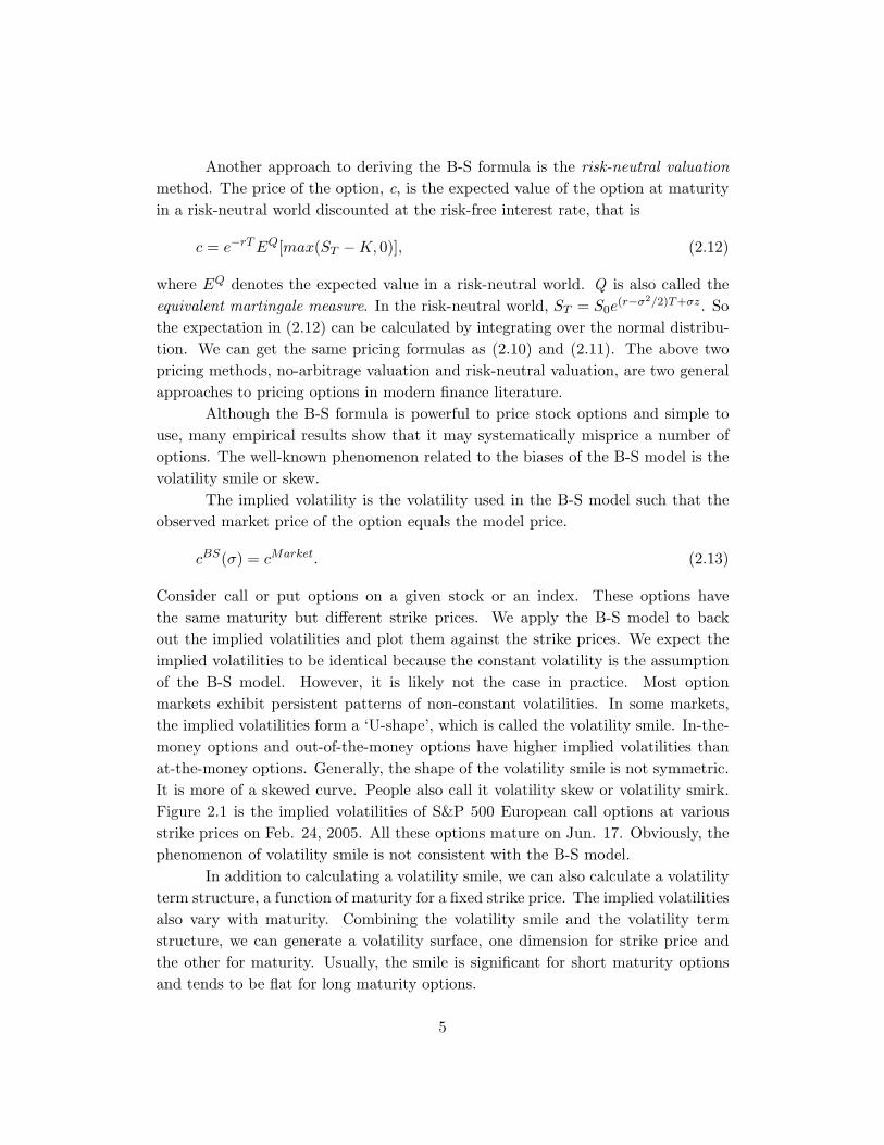
4.3 Implementations and Results

In Figure 4.1 a sample path of stock price under Heston’s model is simulated usingparameters in the Table 4.1. The movement is under the objective measure P.

Table 4.1: Parameters for stock price simulation under Heston’s model

Spot stock price S0 = 1Drift µ = 0.2Time horizon 1 yearRate of mean reversion κ = 2Long-run variance θ = 0.04Spot variance v0 = 0.04Correlation ρ = −0.5Volatility of variance ξ = 0.1

0 0.1 0.2 0.3 0.4 0.5 0.6 0.7 0.8 0.9 10.9

0.95

1

1.05

1.1

1.15Stock Price and Variance Simulation under Heston’s Model

Time

Stoc

k Pr

ice

Stock Price Evolution

0 0.1 0.2 0.3 0.4 0.5 0.6 0.7 0.8 0.9 10.025

0.03

0.035

0.04

0.045

Time

Varia

nce

Variance Evolution

Figure 4.1: Simulation of stock prices under Heston’s model

To exam the effects of some parameters on the option prices, we first considerthe stock price process and the variance process under the equivalent martingalemeasure Q. From section 4.1 , the risk-neutralized process for the variance is

dvt = κ∗(θ∗ − vt)dt + ξ√

vtdZ2t, (4.26)

where κ∗ = κ + λ and θ∗ = κθ/(κ + λ). The variance moves towards a long-runaverage variance θ∗, with a speed determined by κ∗. An increase in θ∗ can increaseoption prices. And κ∗ determines the relative weights of the spot variance and the

22

long-run average variance. The process (4.26) is employed if we want to price optionsby using Monte Carlo simulation.

The closed-form solution (4.6), (4.13), and (4.20)for Heston’s model can beimplemented in some softwares. The solution contains complex numbers. A toolpack for the complex arithmetics is needed for some softwares, e.g. VBA and C++.But it is slow. A better way is to code the arithmetics by ourself. Matlab cancalculate the complex numbers directly. I implement the solution in both VBAand Matlab to check the coding correctness. Another problem in the closed-formsolution is the infinite integral. I use Gauss-Laguerre approximation for infiniteintegrals with 18 points. The integrands are oscillating. But when the strike priceis not too far from the stock price, the approximation is reasonable and the error isquite small.

After we can calculate the option prices in Heston’s model, we can investi-gate other model parameters. Here I focus on the two most important parameters:correlation ρ and volatility of variance ξ. We want to see whether Heston’s modelcan explain the pricing biases of the B-S model. There are many empirical litera-ture to test SV models, e.g. Bakshi, Cao, and Chen (1997). Usually, researchersuse market data for options and stocks to estimate the model parameters and thenexam the in-the-sample and out-of-the-sample pricing errors. Here I use anotherapproach. First I calculate option prices for a set of different strike prices and time-to-maturities under Heston’s model. Then these option prices are used as inputsto the B-S model and the implied volatilities are backed out. Recall that we usemarket prices to back out the market implied volatilities. We want to see whetherHeston’s model can generate volatility smiles and volatility surfaces as implied bythe market prices.

In Figure 4.2, we investigate the effect of ρ on the implied volatility surfacegenerated under Heston’s model. In Panel A, ρ = 0. Away-from-the-money optionshave higher implied volatilities than near-the-money options. This is consistentwith the ‘smile’ shape of implied volatilities in some financial market, e.g. currencyoptions markets. This observation can be explained by the fat-tailed distributionof returns. We can also find that the ‘smile’ flattens when the time to maturityincreases. This is also consistent with the real financial markets. The B-S modeltends to work well for options with long maturities as a result of the correspondingflattened smile.

In Panel B, ρ is negative. We can find that in-the-money calls have higherimplied volatilities, whereas out-of-the-money calls have lower implied volatilities.This is consistent with the phenomenon of ‘volatility skew’ in some financial markets,especially the equity options markets. Panel C has a positive ρ, which can generate

23

00.5

11.5

22.5

3

0.8

0.9

1

1.1

1.20.199

0.1995

0.2

0.2005

0.201

0.2015

0.202

0.2025

Time to Maturity (in years)

Panel A :Correlation equals 0

Strike Price

Impl

id V

olat

ility

00.5

11.5

22.5

3

0.8

0.9

1

1.1

1.20.19

0.195

0.2

0.205

0.21

0.215

Time to Maturity (in years)

Panel B :Correlation equals −0.5

Strike Price

Impl

id V

olat

ility

00.5

11.5

22.5

3

0.8

0.9

1

1.1

1.20.185

0.19

0.195

0.2

0.205

0.21

0.215

Time to Maturity (in years)

Panel C :Correlation equals 0.5

Strike Price

Impl

id V

olat

ility

Figure 4.2: A plot of implied volatilities for option prices under Heston’s model.Strike prices vary between 0.8 to 1.2. Time to maturities are between 0.2 year to 3years. S = 1, r = 0.01, κ = 2, θ = 0.04, v0 = 0.04, ξ = 0.1, λ = 0. Three differentcorrelations ρ are shown.

24

an opposite skew shape compared with Panel B. Such kind of volatility skew mayappear in energy options markets.

The effect of ξ is investigated in Figure 4.3 for different correlations. We canfind that ξ controls the significance of the ‘smile’ or the ‘skew’. A small ξ results ina flat smile, while a large ξ gives us a significant smile.

From the viewpoint of the return distribution, the parameter ρ is related tothe skewness. A negative ρ corresponds to a distribution with a negative skewness.Empirical findings show that stock prices usually have a negative skewness. If themodel only allows ρ = 0, we cannot generate a skewed volatility surface. So Heston’smodel is better than the Hull-White model as Hull and White give a closed-formsolution only for the case ρ = 0. The parameter ξ is related to the kurtosis ofthe distribution. Stock price distribution is found to be leptokurtic, which meansthe return distribution has fatter tails compared with the normal distribution. So apositive ξ is also important to capture the return distribution implied by the marketprices.

4.4 Estimation of Parameters

Heston’s model can capture the smile effect. However, to apply Heston’s model,or other SV models, we need to know the model parameters. Strike price K andtime to maturity T are specified in the contract. And We know spot stock price St,interest rate r from the market. However, the spot variance and its related structuralparameters (κ, θ, ξ, ρ) are unobservable and need to be estimated. Market price ofvolatility risk λ is also unknown. Estimation of these parameters is not an easytask. The likelihood functions are not known in closed form for continuous-time SVmodels, since the observations are discrete. So the maximum likelihood method isvery difficult to implement.

There are several econometric literature on estimation of SV models. Onecan use the underlying stock prices only to estimate the structural parameters. Indi-rect inference method is first proposed by Gourieroux, Monfort, and Renault (1993).This method is a simulation based moment matching method. Some studies have ap-plied indirect inference method to the SV models. Ait-Sahalia and Kimmel (2004)use closed-form approximations to the true but unknown likelihood function andthen employ the maximum likelihood method. Alternatively, researchers extractthe variance from option prices. For example, the implied volatility of at-the-moneyoptions are used to be a proxy for the instantaneous volatility of the stock. Whena time series of implied volatilities or variances is available, subsequent estimationtechniques can be applied. Frequently used methods for SV models include the gen-

25

0.8 0.85 0.9 0.95 1 1.05 1.1 1.15 1.20.192

0.194

0.196

0.198

0.2

0.202

0.204

0.206

0.208

0.21

0.212Panel A: Correlation equals 0

Strike Price

Impl

id V

olat

ility

BSxi=0.1xi=0.2xi=0.3xi=0.4

0.8 0.85 0.9 0.95 1 1.05 1.1 1.15 1.20.17

0.18

0.19

0.2

0.21

0.22

0.23

0.24Panel B: Correlation equals −0.5

Strike Price

Impl

id V

olat

ility

BSxi=0.1xi=0.2xi=0.3xi=0.4

0.8 0.85 0.9 0.95 1 1.05 1.1 1.15 1.20.17

0.18

0.19

0.2

0.21

0.22

0.23Panel C: Correlation equals 0.5

Strike Price

Impl

id V

olat

ility

BSxi=0.1xi=0.2xi=0.3xi=0.4

Figure 4.3: A plot of implied volatilities for option prices under Heston’s model.S = 1, r = 0.01, κ = 2, θ = 0.04, v0 = 0.04, λ = 0. In each panel, ξ changes from 0to 0.4. When ξ = 0, volatility is constant. We are back to the Black-Scholes world.Three different correlations ρ are shown.

26

eralized method-of-moments (GMM) developed by Hansen and Scheinkman (1995),and the efficient method-of-moments (EMM) proposed by Gallant and Tauchen(1996).

But in practice, it is not convenient to employ these econometric tools. Analternative and popular method is to use option prices directly. The procedure issimple. First, we collect Nt options on the same stock in the same day. These optionshave different time to maturities and strike prices. Let cMarket

i,t be the price of thei -th option, and cModel

i,t be its price determined by the model. The parameters wewant to estimate include structural parameters, κ, θ, ξ, ρ, λ, and the spot variancevt. By the expression of the option price under Heston’s model, we know we canalways choose λ = 0 in practice. The parameter set Φ = {κ, θ, ξ, ρ, vt} is thendetermined by

Φ̂ = arg minΦ

1Nt

Nt∑

i=1

(cMarketi,t − cModel

i,t )2. (4.27)

This procedure is used in Bakshi, Cao, and Chen (1997). But in some cases,we don’t have enough options on the same stock traded in one day. Bates (1996)holds the model parameters constant through time and uses many days of optionprices. This approach also have some problems. The spot variance is a parameterin the model. If we use many days of option prices, we will have a number of spotvariances to estimate, one for each day. The computing time will be demandingsince (4.27) is a non-linear optimization problem. Anyway, these approaches usingloss functions are useful in practice and are not very difficult to implement.

27

Chapter 5

Limitations of Stochastic

Volatility Models

The SV model is superior to the Black-Scholes model. Theoretically, SV modelsmake more realistic assumptions; and empirically, researchers also find the SV modeloutperforms the B-S model in pricing options. But SV models are not great enough.The B-S model is easy to understand and implement. In contrast, SV models are noteasy to use in practice. Further more, SV models cannot eliminate all the pricingbiases. There are some evidence showing that SV models are still misspecified. Someassumptions of SV models may be further relaxed.

In Section 4.4, we introduced some calibration methods. In practice, calibra-tion of SV models is a big problem. Volatility is unobservable. It is very hard toestimate model parameters by the underlying stock prices. One can extract impliedvolatility to be a proxy. But in some cases, options are thinly traded. Bid andask spreads are large. The quoted prices are not reliable. If one use the method ofminimizing the difference between the market prices and the model prices, the com-putation time will be demanding. For many SV models, closed-form solutions arenot available. Some numerical methods are used. But usually it is time-consumingto get the price using these numerical methods. The optimization problem (4.27)is solvable in practice only if the option price under SV models can be computedquickly, because the optimization algorithm involves a number of trial-and-errorloops. Although Heston’s SV option pricing model has a closed-form solution, theinfinite integral is still solved by a numerical method. It is much faster than otherSV models. But the optimization problem is still slow. And there are some problemsin this non-linear optimization problem. For example, the solution might be a localminimum point rather than the global minimum point.

An alternative to the continuous-time SV model is the GARCH option pricing

28

model. GARCH models have an advantage that the current volatility is observablefrom the history of stock prices. The model parameters can be readily estimated bythe discrete observations of stock prices. So the estimation procedure is considerablysimplified. The stock price process and variances are discrete under GARCH optionpricing models. Duan (1995) assumes

lnSt

St−1= r + λ

√ht − 1

2ht +

√htεt, εt|φt−1 ∼ N(0, 1), (5.1)

ht = β0 + β1ht−1 + β2ht−1(εt−1 − θ), (5.2)

where r is the risk-free interest rate. λ can be interpreted as the unit risk premium.φt−1 is the information set till time t–1.

In econometrics, GARCH models are the most successful models to modelthe volatilities of financial time series. But the GARCH option pricing model hasnot been commonly used by traders and finance researchers. They still prefer thecontinuous-time models. Duan (1996) shows that most of the existing bivariate diffu-sion models that have been used to model stock returns and volatilities in SV models,can be represented as limits of a family of GARCH models. So continuous-time SVoption pricing models and GARCH option pricing models are closely related. Basedon this fact, Lewis (2000) models the prices by a bivariate diffusion process, butestimate the parameters of the model using GARCH techniques.

Another weakness of SV models is they model stock prices in a continuouscontext. In the real financial markets, prices exhibit jumps rather than continuouschanges. Large price changes cannot be generated by pure diffusion processes inSV models. Bates (1996) finds that some parameters of Heston’s model need tobe implausibly high when fitting the market data. One explanation for this is theabsence of price jumps. We know the correlation paramter, ρ, controls the levelof skewness and the volatility of variance, ξ, controls the level of kurtosis. Butthe ability of Heston’s model to generate enough short term kurtosis is limited.And a high level of ξ means the short-term kurtosis is very high. Bates (1996)adds Poisson jumps in the stock price process and proposes a so-called stochasticvolatility/jump-diffusion (SVJ) model. Discontinuous price jumps and crashes cangenerate additional skewness and kurtosis. So the SVJ model can generate moredesirable return distributions. Bakshi, Cao, and Chen (1997) also find that the SVJmodel outperforms the SV model, especially in pricing short-maturity options. Pricejumps mainly capture short-term excess kurtosis and skewness, whereas stochasticvolatility captures such moment properties in the long run. However, incorporatingjumps increases the implementation cost.

29

Chapter 6

Conclusion

In this essay, I first introduced the B-S model for pricing options. The phenomenonof volatility smile or skew was described. The implied volatilities from market optionprices vary by strike price and time to maturity. It contradicts to the constantvolatility assumption of the B-S model. A number of empirical studies have revealedthat the true distribution of stock returns is a skewed and leptokurtic distributionrather than a normal distribution. To deal with this problem, researchers havepresented several models that incorporating more realistic features of stock returns.

Particularly, SV models have received remarkable attentions. They are saidto be the next generation of option pricing models. Modelling volatilities in astochastic way corrects the simple constant volatility assumption of the B-S model.By changing the model parameters, almost all kinds of asset distributions can begenerated. Allowing volatility to be stochastic, the model can generate a moreleptokurtic return distribution. A negative skewness can also be generated by anegative correlation between the stock price process and the volatility process. TheSV model can also have an implied volatility surface which is similar to the onegenerated by market data. Therefore, the SV model gives a good modification todescribe the real financial markets.

The market incompleteness is one of the most distinctive features of the SVmodel when we want to price and hedge options. The market price of volatility riskwas introduced when pricing options in SV models. Since a perfect hedging is im-possible in incomplete markets, superhedging, mean-variance hedging and shortfallhedging were introduced.

Among several SV models, Heston’s SV model is the most popular one. Aclosed-form solution was derived by a method based on characteristic functions. Weinvestigated the effects of some important parameters of the model by looking atthe implied volatility surface. Estimation of parameters was also discussed, as thisstep is necessary when we want to implement the model in practice.

30

Although SV models have many good features and are found to correct somepricing biases of the B-S model, SV models have some limitations. A discrete versionof the SV model, the GARCH option model, is said to be easily implemented, sincethe parameters can be estimated from underlying stock prices directly. Price jumpsare found to be very common in financial markets. Adding jumps in the standardmodel can improve the performance. A so-called stochastic volatility/jump-diffusionmodel was introduced.

31

Bibliography

[1] Ait-Sahalia, Y., and Kimmel, R., 2005, “Maximum Likelihood Estimation ofStochastic Volatility Models”, working paper, Princeton University.

[2] Bakshi, G., Cao, C., and Chen, Z., 1997, “Empirical Performance of AlternativeOption Pricing Models”, Journal of Finance, 52, 2003-2049.

[3] Bates, D., 1996, “Jumps and Stochastic Volatility: Exchange Rate ProcessesImplicit in PHLX Deutsch Mark Options”, Review of Financial Studies, 9(1),69-107.

[4] Black, F., and Scholes, M., 1973, “The Pricing of Options and Corporate Lia-bilities”, Journal of Political Economy, 81, 637-659.

[5] Bollerslev, T., 1986, “Generalized Autoregressive Conditional Heteroskedastic-ity”, Journal of Econometrics, 31, 307-327.

[6] Campbell, J., Lo, A., and MacKinlay, C., 1997, The Econometrics of FinancialMarkets, Princeton University Press.

[7] Carr, P., and Madan, D., 1999, “Option Pricing and the Fast Fourier Trans-form”, Journal of Computational Finance, 2(4), 61-73.

[8] Cox, J., and Ross, S., 1976, The Valuation of Options for Alternative StochasticProcesses”, Journal of Financial Economics, 3, 145-166.

[9] Cvitanic, J., Pham, H., and Touzi, N., 1999, “Super-Replication in StochasticVolatility Models with Portfolio Constraints”, Journal of Applied Probability,36, 523-545.

[10] Derman, E., and Kani, I., 1994, “Riding on the Smile”, Risk, 7, 32-39.

[11] Duan, J., 1997, “Augmented GARCH(p,q) Process and Its Diffusion Limit”,Journal of Econometrics, 79, 97-127.

32

[12] Duan, J., 1995, “The GARCH Option Pricing Model”, Mathematical Finance,5(1), 13-32.

[13] Dumas, B., Fleming, J., and Whaley, R., 1998, “Implied Volatility Functions:Empirical Tests”, Journal of Finance, 53, 2059-2106.

[14] Engle, R., 1982, “Autoregressive Conditional Heteroskedasticity with Estimatesof the Variance of UK Inflation”, Econometrica, 50, 987-1008.

[15] Follmer, H., and Sondermann, D., “Hedging of Non-Redundant ContingentClaims”, Contributions to Mathematical Economics, 1986, 205-223.

[16] Follmer, H., and Leukert, P., “Efficient Hedging: Cost versus Shortfall Risk”,Finance and Stochastics, 4, 117-146.

[17] Fouque, J-P., Papanicolau, G., and Sircar, K. R., 2000, Derivatives in FinancialMarkets with Stochastic Volatility, Cambridge University Press.

[18] Gallant, A., and Tauchen, G., 1996, “Which Moments to Match?” EconometricTheory, 12, 657-681.

[19] Gkamas, D., 2001, “Stochastic Volatility and Option Pricing”, QuantitativeFinance, 1, 292-297.

[20] Gourieroux, C., Monfort, A., and Renault, E., 1993, “Indirect Inference”, Jour-nal of Applied Econometrics, 8, S85-S199.

[21] Hansen, L., and Scheinkman, J., 1995, ”Back to the Future: Generating Mo-ment Implications for Continuous-Time Markov Processes”, Econometrica, 63,767-804.

[22] Heston, S., 1993, “A Closed-Form Solution for Options with Stochastic Volatil-ity with Applications to Bond and Currency Options”, Review of FinancialStudies, 6, 327-343.

[23] Heston, S., and Nandi, S., 2000, “A Closed-Form GARCH Option PricingModel”, Review of Financial Studies, 13(3), 585-626.

[24] Hull, J., 2002, Options, Futures, and Other Derivatives, 5th ed., Upper SaddleRiver, NJ: Prentice Hall.

[25] Hull, J., and White, A., 1987, “The Pricing of Options on Assets with StochasticVolatilities”, Journal of Finance, 42, 281-300.

33

[26] Lewis, A., 2000, Option Valuation under Stochastic Volatility with MathematicaCode, Newport Beach, CA: Finance Press.

[27] Merton, R., 1976, “Option Pricing When Underlying Stock Returns are Dis-continuous”, Journal of Financial Economics, 3, 125-144.

[28] Scott, L., 1987, “Option Pricing When the Variance Changes Randomly: The-ory, Estimators, and Applications”, Journal of Financial and QuantitativeAnalysis, 22, 419-438.

[29] Stein, E., and Stein, J., 1991, “Stock Price Distributions with StochasticVolatility: An Analytical Approach”, Review of Financial Studies, 4, 727-752.

34