34

Heat Conduction in Nonlinear Media

Michael M. Tilleman Elbit Systems of America (Kollsman), LLC.,

220 Daniel Webster Highway, Merrimack, NH 03054 USA

1. Introduction

The objective of this chapter is to demonstrate a closed form solution to a unique problem in heat transfer, that of heat transfer in nonlinear media. For this purpose identified are cases in which the nonlinear phenomenon dominates, where properties of a medium exhibit nonlinear response to heating, and the solution methodology is described. Further in this chapter presented is a set of analytical solutions applicable to various geometrical forms including the cases of: infinite and finite cylinders with axisymmetrical source, finite cylinder with axisymmetrical and axially varying sources, slender disk, infinite and finite parallelepiped with centrally symmetric source, finite parallelepiped with axially varying source and the resulting stress due to temperature distribution. In this abstract an example is shown of a solution for a particular case, that of an infinite cylinder. In many cases equations governing the phenomenon of heat transfer are solved assuming constant physical properties of the media concerned. That is where a whole class of closed form solutions is found, if regular boundaries and boundary conditions are provided. However, at instances in which the coefficient of heat conduction, specific heat and thermal diffusivity, are functions of temperature, those solutions are no longer applicable. For those cases another family of closed form solutions is found and described herewith. The analytical solution to the thermally nonlinear problem assumes a certain dependence of the coefficient of thermal conductivity, k, on temperature. This case is usually found in instances of large temperature gradients in media, for instance in active optical materials with intense electro-optical fields. They are realized in laser gain media, nonlinear optical crystals and saturable absorbers. One of the most frequently used host materials for lasers is Yttrium Aluminum Garnet, YAG, in which an inverse proportionality to temperature well approximates measured k values over a vast temperature range. What we applied for the solution of such a problem is the Kirchoff’s transformation ( Joyce, 1975), whereby the heat equation can be linearized and solved. However, the use of this method is limited to materials whose k is integrable in temperature, T. Only for these cases the linearization of the heat equation can be made. For instance in the case of AgGaSe2, a nonlinear optical crystal useful for harmonic generation, the dependence is k=A+B/T ( Aggarwal & Fan, 2005) that is an integrable function in T, therefore solvable by the present method. Evidence has it, though, that most of the known optical crystals have similarly thermal coefficient enabling the use of the present solution. Another strategy used in many of the present solutions is the use of the Green’s function as kernel in the integral expression. Owing to the strong

www.intechopen.com

Developments in Heat Transfer

668

dependence of additional properties of these materials, for instance thermal expansion coefficient and thermal rate of refractive index (dn/dT) on temperature, the solution to the heat transfer problem presents an important tool to understand the reaction of these media to intense heating. The analysis begins by defining the governing equation and the boundary conditions. Governing is the Poisson equation expressed as:

( ) 0k T Q∇ ⋅ ∇ + = (1)

where: k=k(T) is the thermal conductivity and Q is the heat source term defined as deposited power per unit volume. To solve for cylinders or rectangular parallelepipeds either a polar or Cartesian coordinate systems need be considered as necessary.

1.1 Coefficient of thermal conductivity

The coefficient of thermal conductivity is a product of the material density, thermal diffusivity and specific heat. Approximation to theory and the fitting to a broad body of measured values suggest an inverse linear approximation:

( ) 00

Tk T k

T= (2)

where k0 is the coefficient of thermal conductivity at T0 whose values for several materials

are summarized.( Aggarwal et al., 2005) This simple function, similar to that suggested for

Nd:YLF in (Pfistner et al., 1994) and ( Hardman et al., 1999), closely fits theory and agrees

very well with data in the range between cryogenic temperature and 770K. It is worth

mentioning that though the specific approximation of Eq. 2 holds true for some materials,

there are other materials for which alternative approximations may become a better fit.

1.2 The nonlinear poisson equation for a cylinder with axisymmetrical source

Let us consider the Poisson equation of Eq. 1 in cylindrical coordinates, using the expression

for k of Eq. 2:

( ) ( )0, , 0 , , , , 0r z r z

Tk T Q r z

Tϕ ϕ ϕ⎡ ⎤∇ ⋅ ∇ + =⎢ ⎥⎣ ⎦ (3)

Consistent with Kirchoff’s transformation this equation can be rewritten as:

( ) ( ) ( )20 0 , , , , 0 0 , ,

0

1, , ln , ,r z r z r z

Tk T T Q r z k T Q r z

T Tϕ ϕ ϕϕ ϕ∇ ⋅ ∇ + = ∇ + (4)

then one arrives at:

( ) ( )2, , , , , , 0r zK r z Q r zϕ θ ϕ ϕ∇ + = (5)

Being a linear equation in θ where:

( ) ( )0

, ,, , ln

T r zr z

T

ϕθ ϕ = (6)

www.intechopen.com

Heat Conduction in Nonlinear Media

669

and K is a constant:

0 0K k T= (7)

The above notation is cylindrical. Notwithstanding, this linearization holds true for any orthogonal coordinate system. It should be emphasized that Eq. 5 represents any steady-state heat equation, where θ and K may be an arbitrary representation of any compound temperature-heat conduction function. Ultimately this case degenerates to the linear case where the heat conduction coefficient is independent of temperature. Assuming a distributed heat source one has:

02

( , , ) ( , , )P eff

PQ r z f r z

r Lϕ ϕπ= (8)

where P is the power deposited in the medium, rP is the effective radius of the heating zone in the cylinder, Leff is the effective length of the medium which may be, for instance, a cylindrical rod or parallelepiped and f0 is an arbitrary spatial distribution function of the deposited power. The boundary conditions for the problem are prescribed by a given cooling mechanism, which may consist of a coolant fluid or a solid heat sink, and physical surroundings of the device. Typically at least one side of the heated medium is held in good thermal contact with the cooling mechanism. Being either kept in vacuum or exposed to gas the other sides of the medium may be considered insulated due to lack of any considerable heat transfer. At the areas of the rod through which heat flow occurs, say at r=rW, one may specify the boundary by a known temperature, i.e. a Dirichlet condition:

0( , , )WT r z Tϕ = (9)

Otherwise, in the case the heat flux out of the system is known, the boundary is specified by a Neumann condition:

ˆ

Tk q

n

∂ =∂ (10)

and on all the insulated sides the heat flux vanishes, thus:

0ˆ

T

n

∂ =∂ (11)

2. Cylindrical rods

Consistent with Kirchoff’s transformation ( Joyce, 1975) Eq. 5 is expressed in cylindrical coordinates as:

( ) ( ) ( ) ( )2 2

2 2 2, , , , , , , 0

K Kr r z r z K r z Q r z

r r r r z

∂ ∂ ∂ ∂θ ϕ θ ϕ θ ϕ ϕ∂ ∂ ∂ϕ ∂+ + + = (12)

2.1 Rod of finite length

This case is illustrated in Figure 1(a). Sketched is a rod held by two conducting mounts at the ends, surrounded on its perimeter by a source emitting electromagnetic radiation. Such a

www.intechopen.com

Developments in Heat Transfer

670

source may be a black-body emitter, incandescent lamp, light emitting diode or laser, to name a few. The rod absorbs the radiation converting it to heat. In order to approximate cases of: 1) rod with evenly spaced side heating and varying axial heating rate or boundary condition, and 2) end heating with arbitrarily distributed source or boundary conditions, it is sufficient to assume an axisymmetrical case with a finite rod. Then the governing equation becomes:

( ) ( ) ( )2

2, , , 0

Kr r z K r z Q r z

r r r z

∂ ∂ ∂θ θ∂ ∂ ∂+ + = (13)

(a) (b) (c)

Fig. 1. Three cylindrical optical devices: a) rod held by heatsink mounts on both ends with radially symmetrical side induction heaters, b) rod held by a heatsink along its length with end induction heater and c) end induction heated thin disk (dark) with a cap

2.1.1 Side heating The boundary conditions for a rod may model various cooling configurations including conductive and convective cooling means. A possible configuration is conduction cooling, where a heat sink with a mount holds the rod over part of its length. This configuration justifies the assumption of either Dirichlet or Neumann boundary conditions or their combination specified around the rod circumference:

( ) ( ) ( ) ( ) ( ) ( )1 2

, ,,

W W

W

r r r r

T r z r zT r z f z or k T K f z

r r

∂ ∂θ∂ ∂= =

= = = (14)

The Dirichlet boundary condition is particularly suitable for cases where the boundary is held at a set temperature such as the case of heat sinking to Peltier junction or cryogenic cooling. In terms of the function θ it becomes:

( ) ( )1

0

, lnW

f zr z

Tθ = (15)

Then, the Neumann condition is suitable for cases where the boundary provides a certain heat flux across it, as specified in Eq. 14. At the rod ends the facets are assumed insulated, specified by Neumann condition, such that:

Heat Induction

Thin Disk

www.intechopen.com

Heat Conduction in Nonlinear Media

671

0 /2

0z z Lz z

∂θ ∂θ∂ ∂= =

= = (16)

where the origin is at the rod center and z = L/2 is half the rod length. Modeling of the heat source assumes a region confined both radially and axially inside the rod:

( )02 ; 0

2/ 2( , )

0 ; 2

P

P lf r z

r lQ r z

lz

π⎧ ≤ ≤⎪⎪= ⎨⎪ <⎪⎩

(17)

where l is the length of the source region in the rod such that l≤L. To solve the set of equations 13 – 16 it is convenient to employ the Green’s function G(r,z) in which case for the mixed boundary conditions the general solution becomes:

( ) ( ) ( ) ( ) ( )/2 /2

3

0 0 0

1, , , , , , , ,

WrL L

W Wr z r f V r z r d Q G r z d dK

θ ζ ζ ζ ξ ζ ξ ζ ξ ξ ζ= +∫ ∫ ∫ (18)

where the function f3(ζ) assumes either f1(ζ) or f2(ζ) defined in Eq. 14 and the function

V(r,z,rW,ζ) is either ∂G(r,z,ξ,ζ)/∂ξ at ξ=rW or G(r,z,rW,ζ), depending on the type of boundary condition around the rod circumference (Dirichlet or Neumann). Green’s function is constructed by solving the homogeneous Eq. 13, or the Laplace equation, satisfying the specified boundary conditions of Eqs.14 and 16, and by the function holding throughout the domain.( Polianin, 2002) Thus G takes the form as demonstrated in (Polianin, 2002):

( ) ( ) ( )( )

0 , 0 ,

2 21 1 2 2

, ,

cos 2 cos 22

, , ,2

s m s m

sm nW

s m s s m W

zJ r J n n

L LG r z

r L nJ r

L

ζμ μ ξ π πξ ζ πμ μ

∞ ∞= =

⎛ ⎞ ⎛ ⎞⎜ ⎟ ⎜ ⎟⎝ ⎠ ⎝ ⎠= ⎡ ⎤⎛ ⎞+⎢ ⎥⎜ ⎟⎝ ⎠⎢ ⎥⎣ ⎦∑ ∑ (19)

where the subscript s assumes the value of either 0 or 1 corresponding to a Neumann or

Dirichlet type boundary condition, respectively. The coefficients μm are the roots of the equation:

( )

( )0

0

0 ; 0

0 ; 1

W

mr

m W

dJ r s

dr

J r s

μμ

= == =

(20)

To present a complete solution one still needs to define the functions f0(r) used in Eq. 17. Let two cases be considered: 1. Uniform heat source distribution where:

( )0

1 ; 0

0 ; P

P

r rf r

r r

≤ ≤⎧= ⎨ <⎩

2. Gaussian heat source profile:

www.intechopen.com

Developments in Heat Transfer

672

( ) 2

0 exp 2P

rf r

r

⎡ ⎤⎛ ⎞⎢ ⎥= − ⎜ ⎟⎢ ⎥⎝ ⎠⎣ ⎦

Considering a Dirichlet boundary condition for case 1 one may solve the problem for θ −θW, whereby the first term in Eq. 18 becomes θW and the solution is expressed as:

( ) ( )( ) ( )

( )

/2

120 0

1 1, 0 1,

2 21 1 2 2

1, 1, 1 1,

2, , , ,

cos 2

sin2

pr l

WP

m p m

Wm nW P

m m m W

Pr z G r z d d

r lK

zJ r J r n

P l Lc n

Lr r LK nJ r

L

θ θ ξ ζ ζξ ξπμ μ π

θ ππ πμ μ μ∞ ∞= =

= +⎛ ⎞⎜ ⎟⎛ ⎞ ⎝ ⎠= + ⎜ ⎟ ⎡ ⎤⎝ ⎠ ⎛ ⎞+⎢ ⎥⎜ ⎟⎝ ⎠⎢ ⎥⎣ ⎦

∫ ∫∑ ∑

(21)

Considering a Neumann boundary condition for case (1), and assuming a case where the heat is relieved from the rod by conductive mounts holding the rod perimeter between ±S/2 and ±L/2 Eq. 18, the solution is:

( ) ( ) ( )( )

( )( ) ( )

/2 /2

0 02/2 0 0

1, 0 1,

21 1 2

1, 1 1,

1 0, 0 0,

2

2, , , , , , ,

sin cos 22

cos

sin

prL lB abs

W WPS

m mB

W m nm m W

m p m

W P

q Pr z r G r z r d G r z d d

K r lK

J rq S S zc n n

K r L L LnJ r

L

J r J rP l

c nLr r LK

ηθ ζ ζ ξ ζ ζξ ξπμ μπ ππμ μμ μ

ππ

∞ ∞= =

= +⎛ ⎞ ⎛ ⎞= ⎜ ⎟ ⎜ ⎟⎡ ⎤⎝ ⎠ ⎝ ⎠⎛ ⎞+⎢ ⎥⎜ ⎟⎝ ⎠⎢ ⎥⎣ ⎦

⎛ ⎞+ ⎜ ⎟⎝ ⎠

∫ ∫ ∫∑ ∑

( )21 1 2 2

0, 0, 0 0,

2

2m nm m m W

zn

L

nJ r

L

ππμ μ μ

∞ ∞= =

⎛ ⎞⎜ ⎟⎝ ⎠⎡ ⎤⎛ ⎞+⎢ ⎥⎜ ⎟⎝ ⎠⎢ ⎥⎣ ⎦∑ ∑

(22)

where qB is the heat flux through the cooling mounts. For a very long rod the solutions in Eqs. 21 and 22 approach the asymptotic solution for a two dimensional, axisymmetrical geometry, which for the Dirichlet boundary condition becomes:

( )22

2

2

exp 1 ; 04

2

;

eff

eff

P

L KW

PP eff P

Peff WL KW

P W

r P rr r

r L K rPT r T

L hrr

r r rr

π

π

ππ∞

⎧ ⎡ ⎤⎛ ⎞⎛ ⎞⎪ − ≤ ≤⎢ ⎥⎜ ⎟⎜ ⎟⎪ ⎜ ⎟⎛ ⎞ ⎢ ⎥⎪⎝ ⎠ ⎝ ⎠⎣ ⎦⎜ ⎟= + ⎨⎜ ⎟⎪⎝ ⎠ ⎛ ⎞⎪ < ≤⎜ ⎟⎪ ⎝ ⎠⎩

(23)

For the heat source of case 2 with Gaussian radial distribution the integrand becomes a product of Bessel function of the first kind of order zero and Gauss function. Then, the integral in the second term of Eq. 18 becomes:

( )00exp 2

Wr

mP

J dr

ξμ ξ ξ ξ⎡ ⎤⎛ ⎞−⎢ ⎥⎜ ⎟⎢ ⎥⎝ ⎠⎣ ⎦∫ (24)

www.intechopen.com

Heat Conduction in Nonlinear Media

673

which has a closed form solution strictly for the case of rW→∞, being ( Abramowitz &

Stegun, 1964):

( )22

exp4 8

m PP rr μ⎡ ⎤⎢ ⎥−⎢ ⎥⎣ ⎦ (25)

It turns out that for rW/ rP =1, 1.25, 1.5, 1.75 the above result has an error of 15%, 6%, 1.5%

and less than 1% relative to a numerical approximation, respectively. Because in real

scenarios rW/ rP >1, this result is applicable to the present solution assuming a Dirichlet

boundary condition, yielding:

( ) ( ) ( )( )

20 1,

1,

2 21 1 2 2

1, 1 1,

cos 2

, exp sin84 2

mm P

Wm nW

m m W

zJ r n

rP l Lr z c n

Lr LK nJ r

L

μ πμθ θ ππ πμ μ∞ ∞= =

⎛ ⎞⎡ ⎤ ⎜ ⎟⎛ ⎞ ⎝ ⎠⎢ ⎥= + − ⎜ ⎟⎢ ⎥ ⎡ ⎤⎝ ⎠ ⎛ ⎞⎣ ⎦ +⎢ ⎥⎜ ⎟⎝ ⎠⎢ ⎥⎣ ⎦∑ ∑ (26)

The temperature in the cylinder for each case is derived via Eq. 6 using the values of θ in

Eqs.21, 22 and 26.

2.1.2 End heating

This case is illustrated in Figure 1(b). Treating the problem of end heating is not much different than the above model for side heating. The main difference is in defining the heat source as an exponentially decaying function along the rod axis. Thus in end heating the

temperature becomes maximized at the rod facet. The temperature surge is milder if an end-cap made up of a non-heating material, is bonded to the rod at the entrance. A non-heating material may be one which does not contain a heat source. The non-heating end-cap conducts the heat generated in the rod. Assumed in the present model is an identical

coefficient of thermal conductivity in the heating and non- heating materials. For the sake of smooth transition from the previous section a notation is selected such where L/2 expresses the entire rod length. In sum the heat source in the rod becomes:

( )02

0 ;2

( , ) exp ; 0 02 2

0 ;

C

C C PP

P

Lz z

P L LQ r z z z f r z z r r

r

r r

α απ

⎧ − <⎪⎪ ⎡ ⎤⎪ ⎛ ⎞= − − − ≤ ≤ − ∩ ≤ ≤⎨ ⎜ ⎟⎢ ⎥⎝ ⎠⎣ ⎦⎪⎪ <⎪⎩

(27)

where zC is the thickness of the end cap, becoming zero for the case with no cap. As in the

previous section also here considered are two cases of radial heat induction distribution: a

flat-top beam and Gaussian. Also cooling of the rod is modeled by assuming either setting

the radial rod wall at a constant temperature or by a conductive mount holding the rod

between the lengths of S/2 and L/2 on each side.

The solution for a rod with uniform heat source and Dirichlet conditions on the cylinder

circumference becomes:

www.intechopen.com

Developments in Heat Transfer

674

( )( )

( ) ( )( ) ( )( )

2

2

1 1, 0 1,

221 1 2 2 1, 1 1,2

1,

2,

21 cos 2 sin 2 exp

2 cos 2

22

WP W

n C CC

m P m

m n m m Wm

LPr z

r r K

z zn Ln n z

J r J rL L L zn

LJ rnn L

L

αθ θ πππ π α μ μα πμ μππ α μ

∞ ∞= =

= +⎧ ⎫⎡ ⎤ ⎡ ⎤⎛ ⎞ ⎛ ⎞ ⎛ ⎞− + − − −⎨ ⎬⎜ ⎟⎜ ⎟ ⎜ ⎟⎢ ⎥ ⎢ ⎥⎝ ⎠⎝ ⎠ ⎝ ⎠ ⎛ ⎞⎣ ⎦⎣ ⎦⎩ ⎭× ⎜ ⎟⎡ ⎤ ⎝ ⎠⎛ ⎞⎡ ⎤+ +⎢ ⎥⎜ ⎟⎣ ⎦ ⎝ ⎠⎢ ⎥⎣ ⎦

∑ ∑ (28)

Considering the Neumann boundary condition the solution is expressed as:

( ) ( ) ( )( )

( )( ) ( )

/2 /2

0 02/2 0 0

1, 0 1,

21 1 2

1, 1 1,

1 0, 0 0,

2

0, 0,

2, , , , , , ,

sin cos 22

sin

prL lB

W WPS

m mB

W m nm m W

m p m

W Pm

q Pr z r G r z r d G r z d d

K r lK

J rq S S zc n n

K r L L LnJ r

L

J r J rP lc n

Lr r LK

θ ζ ζ ξ ζ ζξ ξπμ μπ ππμ μ

μ μππ μ μ

∞ ∞= =

= +⎛ ⎞ ⎛ ⎞= ⎜ ⎟ ⎜ ⎟⎡ ⎤⎝ ⎠ ⎝ ⎠⎛ ⎞+⎢ ⎥⎜ ⎟⎝ ⎠⎢ ⎥⎣ ⎦

⎛ ⎞+ ⎜ ⎟⎝ ⎠

∫ ∫ ∫∑ ∑

( )21 1 2 2

0 0,

cos 22m n

m m W

zn

LnJ r

L

ππ μ∞ ∞= =

⎛ ⎞⎜ ⎟⎡ ⎤ ⎝ ⎠⎛ ⎞+⎢ ⎥⎜ ⎟⎝ ⎠⎢ ⎥⎣ ⎦∑ ∑

(29)

Finally, the solution for a rod with a Gaussian heat source and Dirichlet conditions on the cylinder circumference becomes:

( )( ) ( )

( ) ( )( )( )

2

2

2

1

0 1,

221 1 2 2 1 1,2

1,

,2

2exp 1 cos 2 sin 2 exp

8 2

cos 22

2

WW

m p n C CC

m

m n m Wm

LPr z

r K

r z zn Ln n z

L L LJ r z

nLJ rn

n LL

αθ θ πμ ππ π αα μ πμππ α μ

∞ ∞= =

= +⎡ ⎤ ⎧ ⎫⎡ ⎤ ⎡ ⎤⎛ ⎞ ⎛ ⎞ ⎛ ⎞⎢ ⎥− − + − − −⎨ ⎬⎜ ⎟⎜ ⎟ ⎜ ⎟⎢ ⎥ ⎢ ⎥⎢ ⎥ ⎝ ⎠⎝ ⎠ ⎝ ⎠ ⎣ ⎦⎣ ⎦⎩ ⎭⎢ ⎥ ⎛ ⎞⎣ ⎦× ⎜ ⎟⎡ ⎤ ⎝ ⎠⎛ ⎞⎡ ⎤+ +⎢ ⎥⎜ ⎟⎣ ⎦ ⎝ ⎠⎢ ⎥⎣ ⎦

∑ ∑ (30)

2.2 Example for a cylindrical rod Several cases are calculated showing the profiles of temperature in nonlinear materials. To allow a reasonable comparison between the various cases the following parameters are set: material Yb:YAG, rod diameter 5 mm, radiation absorbing zone diameter 2.5 mm and cryogenic cooling at 77K. Assumed is a circumferential, radially directed radiation forming a uniform heat zone. To estimate the effect of the rod aspect ratio on the axial temperature distribution let a heat density of 410 W/cm3 be set while varying the rod length. Plotted in Figure 2(a) is the axial temperature for half a rod from center to facet with a varying length. Observe that for short rods the temperature is relatively small, growing with length to an asymptotic value. Further length increase causes the temperature profile to flatten out reaching an asymptotic value set by an infinitely long rod. A length of 50 mm may be considered as the value at which the rod is well approximated by an infinitely long rod. Then, the temperature profile is calculated assuming power magnitudes of P=240, 400 and 800 W and a rod length of 50 mm, corresponding to heat density rates of 245, 410 and 815 W/cm3, respectively. Shown in Figure 2(b) is the radial distribution through a rod center for using finite and infinite rod

www.intechopen.com

Heat Conduction in Nonlinear Media

675

models yielding essentially identical results. Also in Figure 2(b) a comparison is made with a calculation based on the linear solution where k is assumed constant equal to that for the median temperature in the rod. In Figure 2(c) plotted are the temperature radial profiles for all three heat density levels, compared again to the linear approach, exhibiting a gradually growing discrepancy between the two for large power levels. It follows that the linear approach is unjustifiable for large heat loads, say above 200 W/cm3.

(a)

(b) (c)

Fig. 2. Temperature in a rod: a) axial distribution for heat density of 410 W/cm3, b) radial distribution for heat density of 410 W/cm3, comparing rod with finite and infinite length and with the linear solution, and c) radial distribution for heat density of 245, 410 and 815 W/cm3, comparing the nonlinear with linear solutions

2.3 Heated thin disk

Illustrated in Figure 1(c), the heated disk experiences greatly diminished radial temperature gradients due to its large area at an axial end being cooled. The thermal problem is solved as in the section above with the difference that here one of the axial facets is attached to a heat sink thus setting the temperature. The other facet is assumed either insulated or bonded to a non-heating layer, a cap. Specifying the boundary conditions for the disk radial wall is twofold: it is insulated for a non-heating disk whereas for a capped disk it has a set temperature, same as the heat-sunk end. Note that for the case of the uncapped end there is no substantial advantage to adding thermal contact to the radial wall due to the large aspect

www.intechopen.com

Developments in Heat Transfer

676

ratio of the disk. On the other hand, for the capped-end case radial cooling must be assumed to render the cap useful. Further assumed is a heat source with flat-top profile enveloped by a circular cylinder with a radius of rP. Denoting the disk thickness as t the heat source density is expressed as:

( ) 2

0 ;

; 0

0 ;

C

pP

p

t z z

PQ r r r

r t

r r

π⎧ − <⎪⎪= ≤ ≤⎨⎪⎪ <⎩

(31)

Then, the boundary conditions are:

( ) ( )( )W

, ,0 ; 0 for uncapped disk

, for capped disk

Wz t r r

W

r z r z

z r

r z

∂θ ∂θ∂ ∂

θ θ= =

= ==

(32)

and the end cooled boundary condition becomes:

( ),0 Wrθ θ= (33)

Green’s function for the Neumann and Dirichlet cases denoted by the subscript s (=0, 1) becomes:

( ) ( ) ( )( )

0 0

2 21 0 2 2

1 1sin sin

2 22, , ,

1

2

sm sm

sm nW

sm s sm W

zJ r J n n

t tG r z

r tn J r

t

ζμ μ ξ π πξ ζ πμ μ

∞ ∞= =

⎡ ⎤ ⎡ ⎤⎛ ⎞ ⎛ ⎞+ +⎜ ⎟ ⎜ ⎟⎢ ⎥ ⎢ ⎥⎝ ⎠ ⎝ ⎠⎣ ⎦ ⎣ ⎦= ⎧ ⎫⎡ ⎤⎪ ⎪⎛ ⎞+ +⎨ ⎬⎜ ⎟⎢ ⎥⎝ ⎠⎣ ⎦⎪ ⎪⎩ ⎭∑ ∑ (34)

Thereby the solution takes the form:

( ) ( ) ( )( ) ( ) ( )

( )

0 0

1 , 0 ,

2 2 21 1 2 2

, , 0 ,

1, , , , ,

1 11 sin 1 sin

2 24

2 1 1

2

Wr t

s W s

n Cs m p s m

Wm nW p

s m s m s m W

r z Q G r z d dK

z zn J r J r n

t tP

nr r tKn J r

t

θ θ ξ ζ ξ ζ ζξ ξπ μ μ π

θ π πμ μ μ∞ ∞= =

= +⎡ ⎤ ⎡ ⎤⎛ ⎞ ⎛ ⎞− + − +⎜ ⎟ ⎜ ⎟⎢ ⎥ ⎢ ⎥⎝ ⎠ ⎝ ⎠⎣ ⎦ ⎣ ⎦= + + ⎧ ⎫⎡ ⎤⎪ ⎪⎛ ⎞+ +⎨ ⎬⎜ ⎟⎢ ⎥⎝ ⎠⎣ ⎦⎪ ⎪⎩ ⎭

∫ ∫∑ ∑

(35)

with the physical stipulation that for s=0 zC=0. Thence the temperature is derived as:

( ) ( ) ( ) ( )( )

1 , 0 ,

2 2 21 1 2 2

, , 0 ,

1 11 sin 1 sin

2 24, exp

2 1 1

2

n Cs m p s m

s Wm nW p

s m s m s m W

z zn J r J r n

t tPT r z T

nr r tKn J r

t

π μ μ ππ πμ μ μ

∞ ∞= =

⎧ ⎫⎡ ⎤ ⎡ ⎤⎛ ⎞ ⎛ ⎞⎪ ⎪− + − +⎜ ⎟ ⎜ ⎟⎢ ⎥ ⎢ ⎥⎪ ⎪⎪ ⎪⎝ ⎠ ⎝ ⎠⎣ ⎦ ⎣ ⎦= ⎨ ⎬+ ⎧ ⎫⎪ ⎪⎡ ⎤⎪ ⎪⎛ ⎞+ +⎨ ⎬⎜ ⎟⎪ ⎪⎢ ⎥⎝ ⎠⎣ ⎦⎪ ⎪⎪ ⎪⎩ ⎭⎩ ⎭∑ ∑ (36)

Evidently the temperature grows exponentially with the dissipated heat density.

www.intechopen.com

Heat Conduction in Nonlinear Media

677

(a) (b)

(c) (d)

(e) (f)

(g) (h)

Fig. 3. Radial and axial temperature profiles in a thin disk assuming a cap length of 0 (a,b), 0.25 mm (c,d), 0.75 mm (e,f) and 1.25 mm (g,h)

www.intechopen.com

Developments in Heat Transfer

678

2.4 Example for a thin disk

To calculate the temperature in the disk the following parameters are set: material Yb:YAG, disk diameter 5 mm, heat source diameter or thickness 2.5 mm, slab lengths 50 mm, disk thickness 0.25 mm, heat density rate 100 W/cm3 and cryogenic cooling at 77K. Consistent with most realistic scenarios consider end heating of the thin disk with uniform radial distribution within a radius of rP of a disk attached to a heat sink. To enhance heat dissipation assumed is also a non-heating cap in good thermal contact with the disk and a heat sink around its perimeter. For simplicity the cap is considered possessing the identical values of coefficient of thermal conduction of the absorbing disk. Thus attached to the disk with the thickness of 0.25 mm is a cap with a varying thickness of 0, 0.25, 0.75 and 1.75 mm. For a heat sink temperature of 77K, disk diameter of 5 mm, source diameter of 2.5 mm and power P=400 W the temperature axial and radial profiles are plotted in Figure 3. On inspecting the graphs (a) – (h) one finds a dramatic drop in the maximum temperature of above 300K to below 90K resulting from increasing the cap thickness from nil to 1.75 mm. Another interesting point is that the axial location of the hottest spot remains at roughly the

doped disk facet. Next, the axial and radial profiles of Δn radial component are plotted in

Figure 3. On inspecting the graphs (a) – (h) one finds a dramatic decrease in the Δn

magnitude from 2.5×10-3 to below 4×10-5 with increasing the cap thickness. Also the axial

location of the peak Δn remains at the doped disk facet.

3. Slab geometry

For active optical media having the shape of a parallelepiped it is most convenient to treat Eq. 5 in Cartesian coordinates, where consistent with Kirchoff’s transformation ( Joyce, 1975) it is expresses as:

( ) ( )2 2 2

2 2 2, , , , 0K x y z Q x y z

x y zθ⎛ ⎞∂ ∂ ∂+ + + =⎜ ⎟⎜ ⎟∂ ∂ ∂⎝ ⎠

(37)

3.1 Slab of infinite length The case of a very long slab relative to its lateral sides is well approximated by an infinitely long slab is schematically shown in Figure 4(a). Here the slab is held on one side in thermal contact with the heat sink, having its width in the z direction and thickness in x direction, both much shorter than its length in the y direction. Heating sources such as lasers, emit radiation which forms inside the slab a laser gain zone a fraction of which generates heat due to the quantum defect and other non-radiative relaxation processes. Considered is a side-heated model having a slander spot shape on the slab side. It has predominantly a Gaussian intensity distribution in the fast-axis plane, i.e. along x, and a uniform distribution along y. I choose to specify the boundary conditions as:

00

( , ) ( , ) ( , )0

xy y b

T x y T x y T x y

y y x == =∂ ∂ ∂= = =∂ ∂ ∂ (38)

and:

( , ) WT a y T= (39)

www.intechopen.com

Heat Conduction in Nonlinear Media

679

where TW is the temperature of the heat-sink at the interface with the slab wall. In the notation

of the non-dimensional temperature θ the two-dimensional Poisson equation becomes:

( ) ( )2 2

2 2

,, 0

Q x yx y

Kx yθ⎛ ⎞∂ ∂+ + =⎜ ⎟⎜ ⎟∂ ∂⎝ ⎠

(40)

with the boundary conditions thus converted to:

00

( , ) ( , ) ( , )0 ; ( , ) W

xy y b

x y x y x ya y

y y x

θ θ θ θ θ== =

∂ ∂ ∂= = = =∂ ∂ ∂ (41)

For a constant θW this allows a solution for the function ( , ) Wx yθ θ− with a zero boundary value at x=a. Assumed for this case is a heat source:

( ) ( )0( , ) exp2 P

PQ x y y f x

r L

α α= − (42)

where α is the absorption coefficient of the laser radiation, rP is the small aperture of the radiation beam, a, b and L are the x , y and z dimensions of the slab (a,b<<L). If the slab side at y=b reflects the inducing beam then the heat source becomes:

( ) ( ) ( )0

exp( , ) cosh

P

P bQ x y b y f x

r L

α α α− ⎡ ⎤= −⎣ ⎦ (43)

The formal solution to the equation set 40 – 41 is:

( ) ( ) ( )0 0

1, , , , ,

a b

Wx y Q G x y d dK

θ θ ξ η ξ η ξ η= + ∫ ∫ (44)

where the Green’s function construction is stipulated by solving the homogeneous Eq. 40, or the Laplace equation, by satisfying the boundary conditions and by its holding throughout the domain. It results in:

( ) ( ) ( ) ( ) ( )2 2

1 0

cos cos sin sin4, , , l l m m

l m l m

p y p q x qG x y

ab p q

η ξξ η ∞ ∞= =

= +∑ ∑ (45)

where:

1;

2l m

lp q m

b a

π π ⎛ ⎞= = +⎜ ⎟⎝ ⎠ (46)

To present a complete solution one still needs to define the functions f0(x) used in Eq. 42. Let two cases be considered: 1. uniform heat source distribution in the x axis where:

( )0

1 ; 2 2

0 ; 2 2

P P

P P

a ar x r

f xa a

x r r x

⎧ − ≤ ≤ +⎪⎪= ⎨⎪ < − ∩ + <⎪⎩

www.intechopen.com

Developments in Heat Transfer

680

2. Gaussian heat source profile:

( ) 2

0

/2exp 2

P

x af x

r

⎡ ⎤⎛ ⎞−⎢ ⎥= − ⎜ ⎟⎢ ⎥⎝ ⎠⎣ ⎦

Considering case (1), Eq. 44 is integrated to the closed form solution:

( ) ( ) ( )( )( ) ( ) ( )2

2 2 2 20 0

1 1 sin sin2

, 4 cos sin

l b mm P

W l mP l m m l l m

q ae q r

Px y p y q x

r abLK q p p q

ααθ θ α−∞ ∞

= =

⎛ ⎞⎡ ⎤− − ⎜ ⎟⎣ ⎦ ⎝ ⎠= + + +∑ ∑ (47)

when no electromagnetic radiation is reflected from slab end, and to:

( ) ( ) ( )( )( ) ( ) ( )2

2 2 2 20 0

sinh( )sin sinexp 2

, 8 cos sin

ml m P

W l mP l m m l l m

q ap b q r

P bx y p y q x

r abLK q p p q

α αθ θ α∞ ∞= =

⎛ ⎞⎜ ⎟− ⎝ ⎠= + + +∑ ∑ (48)

when the electromagnetic radiation is fully reflected from slab end. Then for case (2) the solution takes the form:

( ) ( )( )( )( )

( ) ( )( )( )( )

( )

2

2

28

2 2 2 21 0

2 2

28

2 2 2 20

1 1, 4 2 sin

2

2 2erf erf cos sin

2 2 2 2

1 18 2 sin

2

m P

m P

q rl bm

Wl m m l m

m P m Pl m

P P

q rl bm

Wm m l m

e q aPx y e

abLK p p q

iq r a iq r ap y q x

r r

e q aPe

abLK p p q

α

α

αθ θ π α

αθ π α

−∞ ∞ −= =

−∞ −=

− − ⎛ ⎞= − ⎜ ⎟⎝ ⎠+ +⎡ ⎤⎛ ⎞ ⎛ ⎞− −× −⎢ ⎥⎜ ⎟ ⎜ ⎟⎜ ⎟ ⎜ ⎟⎢ ⎥⎝ ⎠ ⎝ ⎠⎣ ⎦

− − ⎛≈ − ⎜⎝+ +

∑ ∑

∑ ( ) ( )

( )( ) ( )

( )

2 2

2

1

1

4

21 2

cos sin

2erf 1 cos 2 1 cosh cos

22 4

sinh sin2

P P

l ml

a anr r

m Pm m

P Pn

PP

m Pm

p y q x

nq ra e e e aq a q a

ar ranr r

nq rn q a

ππ

∞=

⎛ ⎞ ⎛ ⎞− −⎜ ⎟ ⎜ ⎟ −∞⎝ ⎠ ⎝ ⎠=

⎞⎟⎠⎧⎪ ⎡⎛ ⎞ ⎛ ⎞⎪ ⎛ ⎞× + − + −⎨ ⎜ ⎟ ⎢ ⎜ ⎟⎜ ⎟⎝ ⎠⎝ ⎠⎝ ⎠ ⎛ ⎞ ⎣⎪ + ⎜ ⎟⎪ ⎝ ⎠⎩

⎫⎤⎛ ⎞ ⎪+ ⎬⎥⎜ ⎟⎝ ⎠ ⎪⎦⎭

∑

∑

(49)

where pm is defined in Eq. 46. On inspecting Eqs. 47 and 49 one observes that for a>>rP the solution is insensitive to the magnitude of rP.

3.2 Slab of finite length

The heat conduction problem in a slab of finite length is three dimensional, covering the cases illustrated by Figure 4(a) and (b), where a slab is held on one side in thermal contact with a heat sink and is either side heated (a), or end heated (b). The coordinate system is chosen to represent length in z axis and comparable width sizes in x and y axis. The governing equation is the Poisson equation in Cartesian coordinates, with respect to all three axes as given in Eq. 37. Several configurations of heat inductions are considered:

www.intechopen.com

Heat Conduction in Nonlinear Media

681

1) side heat induction in the y direction where the source has an oblong spot shape and a Gaussian intensity distribution in x, 2) side heat induction with alternating directions of + y and –y, and 3) end heat source in the z direction having a circular spot shape and Gaussian intensity distribution. Also solved is a case for a heat source additional to that occurring in the heating path, which originates from fluorescence and photon trapping in the slab bulk and walls. Finally, several cases of slab cooling are considered: 1) contact with heat sink on one of the slab sides, 2) contact with heat sink on two of the slab sides, and 3) contact with heat sink on all four of the slab sides.

(a) (b)

Fig. 4. Two parallelepipeds: a) slab attached to a heatsink on one side, with a slender side

pump and, b) slab attached to heatsink on one side with an end pump

3.2.1 Side heating

In this case the crystal is considered three dimensional, in thermal contact with a heat sink

on one side, thus there are five Neumann and a single Dirichlet type boundary conditions.

They are expressed as:

0 00

( , , ) ( , , ) ( , , ) ( , , ) ( , , )0

z z L xy y b

x y z x y z x y z x y z x y z

z z y y x

θ θ θ θ θ= = == =

∂ ∂ ∂ ∂ ∂= = = = =∂ ∂ ∂ ∂ ∂ (50)

and: '( , , ) ( , , ) 0Wa y z a y zθ θ θ= − = Consequently the Green’s function becomes:

( ) ( ) ( ) ( ) ( )( ) ( )0 1

cos cos cos cos1, , , , , ,

coshn n m m

nmnm nmn m

p x p q y qG x y z H z

ab L

ξ ηξ η ζ ζβ β∞ ∞= =

= ∑ ∑ (51)

where the function Hnm(z,ζ) is:

( ) ( ) ( )( ) ( )cosh cosh ; 0

,cosh cosh ; 0

nm nmnm

nm nm

L z L zH z

z L L z

β ζ β ζζ β β ζ ζ⎧ ⎡ − ⎤ ≥ > ≥⎪ ⎣ ⎦= ⎨ ⎡ − ⎤ ≥ > ≥⎪ ⎣ ⎦⎩ (52)

and the coefficients pn, qm and βnm are:

www.intechopen.com

Developments in Heat Transfer

682

2 2

1

2; ;n m nm n m

nm

p q p qa b

π π β⎛ ⎞+⎜ ⎟⎝ ⎠= = = + (53)

Further, allowing for a non-absorbing cap having thickness of bC on the radiation side the heat source is defined as:

( ) ( )0

0 ;

( , , )exp , ;

2

C

C CP P

y b

Q x y z Py b f x z b y b

r L

α α<⎧⎪= ⎨ ⎡ ⎤− − ≤ ≤⎣ ⎦⎪⎩

(54)

where LP is the radiation length and the term f0 defines the lateral profile of the source, assumed either as flat top or Gaussian: 1. flat top:

( )0

1 ; 0 0 2

,

0 ; , or 2 2

P P

P P P

ax r z L

f x za a

r x x r L z

⎧ ≤ − ≤ ∩ ≤ ≤⎪⎪= ⎨⎪ + < < − <⎪⎩ (55)

2. Gaussian:

( )2

0

/ 21 ; exp 2 0

,

0 ;

PP

P

x az L

f x z r

L z

⎧ ⎡ ⎤⎛ ⎞−⎪ ⎢ ⎥− ∩ ≤ ≤⎪ ⎜ ⎟= ⎢ ⎥⎨ ⎝ ⎠⎣ ⎦⎪ <⎪⎩ (56)

The formal solution takes the shape:

( ) ( ) ( )0

0 0 0

, , , , , , , , ,a b L

x y z Q G x y z d d dθ θ ξ η ζ ξ η ζ ξ η ζ= + ∫ ∫ ∫ (57)

which after substituting the functions given in Eqs. 51 and 54 and carrying out the integration becomes:

( ) ( ){ }( ) ( )

( ) ( ) ( )( )

2

0 2

2 2 20 1

, ,1 exp

1 1 sin cos2

cos cos

coshtanh sinh

cosh

cz

P C

mn P n

n mn m n m nm

nmnm nm P

nm

P ex y z

r abK b b

ap r p

p x q yp q

zL L L

L

ααθ θ π α

α βββ β β

∞ ∞= =

= + ⎡ ⎤− − −⎣ ⎦⎛ ⎞⎡ ⎤− − ⎜ ⎟⎣ ⎦ ⎝ ⎠× +

⎡ ⎤× − −⎢ ⎥⎣ ⎦

∑ ∑ (58)

Observe that for rP=a/2 the term ( ) ( )sin cos /2n P np r p a becomes ( )1 /2n− , and for L=LP the

term in the square parenthesis becomes merely tanh nmLβ thus rendering the solution in Eq. 58 independent of z.

www.intechopen.com

Heat Conduction in Nonlinear Media

683

Often radiation sources are placed successively on both sides of a slab. In order to solve for

this case one needs only to add a second source placed on the other side of the slab, whereby

the governing equation and boundary conditions remain as stated above, however the heat

source is defined as:

( )( ) ( )0

0 ;

exp( , , ), ;

2 1 exp 2

C C

CC C

P P C

b b y b

b b yQ x y z Pf x z b y b b

r L b b

α αα

− < <⎧⎪ ⎡ ⎤− − −= ⎨ ⎣ ⎦ ≤ ≤ −⎪ ⎡ ⎤− − −⎣ ⎦⎩ (59)

where the term f0 is assumed either flat top:

( )0

1 ; 0 2 2

,

0 ; , or ; 2 2 2

P P P

P P P P

ax r L z L

f x za a

r x x r z L L z

⎧ ≤ − ≤ ∩ ≤ ≤⎪⎪= ⎨⎪ + < < − < <⎪⎩ (60)

The solution to this problem becomes:

( ) ( ){ }( )

( ) ( ) ( )( )

2

0

2 2 20 1

, ,2 1 exp

cos cos sin sin

sin cos cos cos2

cocoshtanh sinh 2 sinh

cosh

c c

B

P P C

b bB Bmm m c m m c

n m n m nm

n P n n m

nmnm nm P nm P

nm

P ex y z

r L abK b b

qe q B e q b e q B e q b

p q

ap r p p x q y

zL L L L

L

α

α αα α

αθ θ αα

α β

ββ β ββ

−

∞ ∞= =

= + ⎡ ⎤− − −⎣ ⎦⎡ ⎤ ⎡ ⎤− + −⎣ ⎦ ⎣ ⎦× +

⎛ ⎞× ⎜ ⎟⎝ ⎠× − − −

∑ ∑

( )sh

coshnm

nm

L z

L

ββ

⎡ ⎤−⎢ ⎥⎣ ⎦

(61)

The complete solution to the slab induced by two sources disposed successively on opposite

sides of the slab is the combination of Eqs.58 and 61. Note that by this technique one can to

arbitrarily add additional induction sources on the slab sides arriving at a closed form

solution for each configuration. Finally, using this solution the temperature is again derived

via Eq. 6.

3.2.2 End heating

Treating the problem of end heat induction is in fact exactly that as the above model for

side heat induction however with changing the characteristics of the source. The heat

source is now considered axisymmetrical with a Gaussian power distribution. In end

heating the temperature is maximized at the slab facet. This surge may be relieved by

bonding to the entrance facet of the slab a non-heating end-cap segment. Lacking a heat

source yet being heat conductive contributes to removing heat from the slab facet. In the

present model it is assumed that the coefficient of thermal conductivity in both materials

is identical. For this case with the radiator aligned to the slab centerline the heat source

term is rewritten as:

www.intechopen.com

Developments in Heat Transfer

684

( )( ) ( )02

0 ;

exp( , , ), ;

1 exp

C

CC

CP

z z

z zQ x y z Pf x y z z L

L zr

α ααπ

<⎧⎪ ⎡ ⎤− −= ⎨ ⎣ ⎦ ≤ ≤⎪ ⎡ ⎤− − −⎣ ⎦⎩ (62)

where f0 is given by:

( ) 2 2

0

/ 2/ 2, exp 2

P P

y bx af x y

r r

⎧ ⎫⎡ ⎤⎛ ⎞ ⎛ ⎞−−⎪ ⎪⎢ ⎥= − +⎨ ⎬⎜ ⎟ ⎜ ⎟⎢ ⎥⎝ ⎠ ⎝ ⎠⎪ ⎪⎣ ⎦⎩ ⎭ (63)

Again, the heat source in the slab can be expressed by Eq. 57, which after substituting the functions given in Eqs.51 and 54 and carrying out the integration becomes:

( ) ( ){ }( ) ( ) ( ) ( )

( )

2

0

0 1

2 2

1, ,

4 1 exp

cos cos, ,

cosh

1cosh cosh sinh

cz

C

n mn n m m

nm nmn m

L znmnm nm nm

nm

P ex y z

abK b b

p x q yF p a F q b

L

L z e z e L

α

α α

αθ θ α

β βββ β βαα β

∞ ∞= =

− −

= + ⎡ ⎤− − −⎣ ⎦×

⎡ ⎤× − − −⎢ ⎥− ⎣ ⎦

∑ ∑ (64)

where:

( ) ( )( )

2

2

2

002

4

20 2

2 2erf

2

, exp cos8 2

1 cos cosh2 2

2

P

a

r

n P n kn n

n Pn

k

P

a ae

rrp r p a

F p akp re

p aa

kr

π⎛ ⎞−⎜ ⎟⎝ ⎠

−∞=

⎧ ⎫⎛ ⎞⎪ ⎪+⎜ ⎟⎪ ⎪⎜ ⎟⎝ ⎠⎪ ⎪⎡ ⎤ ⎛ ⎞⎪ ⎪⎢ ⎥= − ⎨ ⎬⎜ ⎟⎢ ⎥ ⎝ ⎠ ⎡ ⎤⎛ ⎞⎪ ⎪⎣ ⎦ × −⎢ ⎥⎜ ⎟⎪ ⎪⎝ ⎠⎣ ⎦⎛ ⎞⎪ ⎪+ ⎜ ⎟⎪ ⎪⎝ ⎠⎩ ⎭∑ (65)

Note that in the above equation the index n, coefficient pn and length a can be replaced by m, coefficient qm and length b, respectively. Next, the function F can be further simplified considering the values of the coefficients pn and qm as given in Eq. 53 provides the following values:

( )

( ) ( )

1 1 1 1cos , , , ,... for 0,1,2,3,...

2 2 2 2 2

cos 0

cos 0, 1,0,1,... for 1,2,3,4...2

cos 1

n

n

m

mm

p an

p a

q bm

q b

⎛ ⎞ = − − =⎜ ⎟⎝ ⎠=

⎛ ⎞ = − =⎜ ⎟⎝ ⎠= −

(66)

It should be mentioned that the F function is a close approximation to a combination of error functions of complex arguments as shown in (Abramowitz & Stegun, 1964).

www.intechopen.com

Heat Conduction in Nonlinear Media

685

3.2.3 Additional case – slab attached to a heat sink on two sides

Selecting next to carry out the solution for the case of a slab held in thermal contact with a

heat sink on two adjacent walls, the boundary conditions are specified as:

0 0 0

( , , ) ( , , ) ( , , ) ( , , )0

z z L x y

T x y z T x y z T x y z T x y z

z z x y= = = =∂ ∂ ∂ ∂= = = =∂ ∂ ∂ ∂ (67)

and:

( , , ) ( , , ) WT a y z T x b z T= = (68)

Relative to the dimensionless temperature θ the boundary conditions become:

0 00

( , , ) ( , , ) ( , , ) ( , , )0

z z L xy

x y z x y z x y z x y z

z z y x

θ θ θ θ= = ==

∂ ∂ ∂ ∂= = = =∂ ∂ ∂ ∂ (69)

and: ( , , ) ( , , ) 0a y z x b zθ θ= = The formal solution is given by Eq. 57 with the heat source Q given by Eq. 62. The Green’s

function is constructed according to that the rules explained in the previous section, thus

becoming as in Eqs.51 and 52 however with the set of coefficients pn, qm and βnm are

2 21 1: ;

2 2n m nm n mp n q m p q

a b

π π β⎛ ⎞ ⎛ ⎞= + = + = +⎜ ⎟ ⎜ ⎟⎝ ⎠ ⎝ ⎠ (70)

Because both walls attached to the heat sink are held at the uniform temperature of TW, the

solution is identical to that in Eqs.64 and 65 with the difference of the coefficient qm and that

the summation over m begins at 0.

3.2.4 Additional case – slab attached to a heat sink on four sides

In comparison with a slab in contact with a heat sink on two sides a surrounding heat sink on four sides is expected to further lower the temperature elevation due to heating. Unlike in the case where the slab is held by two sides, where the boundary conditions have four Neumann and two Dirichlet type conditions, for this case there are two Neumann and four Dirichlet type conditions expressed as:

0

( , , ) ( , , )0

z z L

x y z x y z

z z

θ θ= =

∂ ∂= =∂ ∂ (71)

and: (0, , ) ( , , ) ( ,0, ) ( , , ) 0y z a y z x z x b zθ θ θ θ= = = = One may approach a solution using symmetry considerations solving in the x and y

coordinates instead of the domain 0→a and 0→b, respectively, in the domain 0→a/2 and

0→b/2. Since in this case the heat source Q given by Eq. 62 is slightly modified to conform with the symmetry consideration such that the f0 function is expressed as:

( ) 2 2

0 , exp 2P P

yxf x y

r r

⎧ ⎫⎡ ⎤⎛ ⎞ ⎛ ⎞⎪ ⎪⎢ ⎥= − +⎨ ⎬⎜ ⎟ ⎜ ⎟⎢ ⎥⎝ ⎠ ⎝ ⎠⎪ ⎪⎣ ⎦⎩ ⎭ (72)

www.intechopen.com

Developments in Heat Transfer

686

In this domain the solution is identical to the case of a slab held by a heat sink on two sides, for which the solution is given by Eq. 64 where the Fn function is expressed as:

( ) ( )( )

2

2

2

02

4

20 2

2 2erf

2

, exp8

1 cos cosh2 2

2

P

a

r

P

n P kn n

n Pn

k

P

a ae

rrp r

F p akp re

p aa

kr

π⎛ ⎞−⎜ ⎟⎝ ⎠

−∞=

⎧ ⎫⎛ ⎞⎪ ⎪+⎜ ⎟⎪ ⎪⎜ ⎟⎝ ⎠⎪ ⎪⎡ ⎤ ⎪ ⎪⎢ ⎥= − ⎨ ⎬⎢ ⎥ ⎡ ⎤⎛ ⎞⎪ ⎪⎣ ⎦ × −⎢ ⎥⎜ ⎟⎪ ⎪⎝ ⎠⎣ ⎦⎛ ⎞⎪ ⎪+ ⎜ ⎟⎪ ⎪⎝ ⎠⎩ ⎭∑

(73)

Further, the set of coefficients pn, qm and βnm as expressed in Eq. 70.

3.3 Example for slab

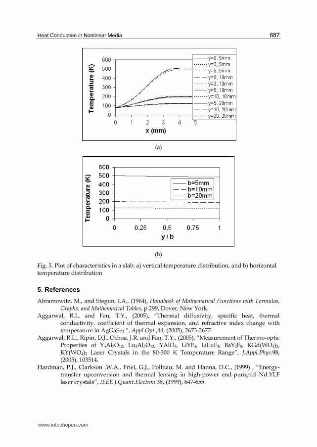
To calculate the temperature in the slab the following parameters are set: material Yb:YAG, square slab side 5 mm, heat source diameter or thickness 2.5 mm, slab lengths 50 mm, heat density rate 100 W/cm3 and cryogenic cooling at 77K. Assumed in this case is a Yb:YAG slab side having heat induced by a flat top beam, with a reflecting opposite wall spaced by a varying width of 5, 10 and 20 mm from the first wall,

where the slab height is 5 mm, its length is 50 mm and the radiation footprint is 2.5×50 mm. The assumed power is P=400 W and the slab is attached to a heat sink held at 77K by its wide side. For the three slab widths the vertical and horizontal temperature distributions are plotted in Figure 5(a) and (b). A considerable variation is found for the vertical temperature whereas horizontal the temperature remains nearly unchanged.

4. Concluding remarks

Closed form solutions to the nonlinear steady-state heat equation in a cylindrical rod, thin disk and parallelepiped are presented. Hinging on using Kirchoff’s transformation, this solution is applicable to any material in which the coefficient of thermal conductivity is integrable in temperature. In turn, these solutions enable solving further the equation of elasticity and that of a propagating optical beam in an inhomogeneous medium where the refractive index is radially modulated. Exemplary calculations are made for a Yb:YAG crystal with temperature spanning the range of 77K – 770K. It is shown that under the condition of large heating loads, say above 200 W/cm3, predicting the temperature according to a linear approximation underestimates the temperature. Thus, in order to obtain accurate results one must use the nonlinear solution arrived at in this study. The predicted temperatures escalate rapidly with thermal loading reaching 120 K and almost 200 K on the optical path for a respective heating by 400 and 800 W, in a cryogenically cooled rod. If the cooling level is raised to room temperature, then by heating the rod at 400 W, the temperature at the center will exceed 700K. Under the heat induction condition of heating at 500 W and cryogenic cooling the maximum temperature reached in a thin disk, having a thickness of ¼ mm, is less than 90K provided it has a cap at least seven times the disk thickness. Without the cap the maximum would exceed 300K. For a slab pumped with identical power and cryogenically cooled on one side the maximal temperature varies between 125K and 500K, depending on the slab width spanning the range from 20 to 5 mm, respectively.

www.intechopen.com

Heat Conduction in Nonlinear Media

687

(a)

(b)

Fig. 5. Plot of characteristics in a slab: a) vertical temperature distribution, and b) horizontal temperature distribution

5. References

Abramowitz, M., and Stegun, I.A., (1964), Handbook of Mathematical Functions with Formulas, Graphs, and Mathematical Tables, p.299, Dover, New York.

Aggarwal, R.L. and Fan, T.Y., (2005), “Thermal diffusivity, specific heat, thermal conductivity, coefficient of thermal expansion, and refractive index change with temperature in AgGaSe2 “, Appl.Opt.,44, (2005), 2673-2677.

Aggarwal, R.L., Ripin, D.J., Ochoa, J.R. and Fan, T.Y., (2005), “Measurement of Thermo-optic Properties of Y3Al5O12, Lu3Al5O12, YAlO3, LiYF4, LiLuF4, BaY2F8, KGd(WO4)2, KY(WO4)2 Laser Crystals in the 80-300 K Temperature Range”, J.Appl.Phys.98, (2005), 103514.

Hardman, P.J., Clarkson ,W.A., Friel, G.J., Pollnau, M. and Hanna, D.C., (1999) , “Energy-transfer upconversion and thermal lensing in high-power end-pumped Nd:YLF laser crystals”, IEEE J.Quant.Electron.35, (1999), 647-655.

www.intechopen.com

Developments in Heat Transfer

688

Joyce, W.B., (1975), “Thermal resistance of heat sinks with temperature-dependent conductivity”, Solid-State Electronics 18, (1975), 321.

Pfistner, C., Weber, R., Weber, H.P., Merazzi, S., and Gruber, R., (1994) , “Thermal beam distortions in end-pumped Nd:YAG, Nd:GSGG and Nd:YLF rods”, IEEE J.Quantum Electron.30, (1994), 1605-1615.

Polianin, A.D., (2002), Handbook of linear partial differential equations for engineers and scientists, Chapman & Hall/CRC.

www.intechopen.com

Developments in Heat TransferEdited by Dr. Marco Aurelio Dos Santos Bernardes

ISBN 978-953-307-569-3Hard cover, 688 pagesPublisher InTechPublished online 15, September, 2011Published in print edition September, 2011

InTech EuropeUniversity Campus STeP Ri Slavka Krautzeka 83/A 51000 Rijeka, Croatia Phone: +385 (51) 770 447 Fax: +385 (51) 686 166www.intechopen.com

InTech ChinaUnit 405, Office Block, Hotel Equatorial Shanghai No.65, Yan An Road (West), Shanghai, 200040, China

Phone: +86-21-62489820 Fax: +86-21-62489821

This book comprises heat transfer fundamental concepts and modes (specifically conduction, convection andradiation), bioheat, entransy theory development, micro heat transfer, high temperature applications, turbulentshear flows, mass transfer, heat pipes, design optimization, medical therapies, fiber-optics, heat transfer insurfactant solutions, landmine detection, heat exchangers, radiant floor, packed bed thermal storage systems,inverse space marching method, heat transfer in short slot ducts, freezing an drying mechanisms, variableproperty effects in heat transfer, heat transfer in electronics and process industries, fission-trackthermochronology, combustion, heat transfer in liquid metal flows, human comfort in underground mining, heattransfer on electrical discharge machining and mixing convection. The experimental and theoreticalinvestigations, assessment and enhancement techniques illustrated here aspire to be useful for manyresearchers, scientists, engineers and graduate students.

How to referenceIn order to correctly reference this scholarly work, feel free to copy and paste the following:

Michael M. Tilleman (2011). Heat Conduction in Nonlinear Media, Developments in Heat Transfer, Dr. MarcoAurelio Dos Santos Bernardes (Ed.), ISBN: 978-953-307-569-3, InTech, Available from:http://www.intechopen.com/books/developments-in-heat-transfer/heat-conduction-in-nonlinear-media