
Hardness Results for Problems P: Class of “easy to solve” problems Absolute hardness results...
28
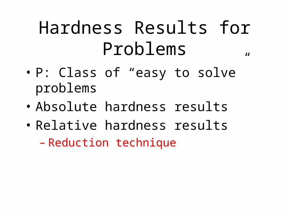
Hardness Results for Problems • P: Class of “easy to solve” problems • Absolute hardness results • Relative hardness results – Reduction technique
-
date post
19-Dec-2015 -
Category
Documents
-
view
213 -
download
0
Transcript of Hardness Results for Problems P: Class of “easy to solve” problems Absolute hardness results...

Hardness Results for Problems
• P: Class of “easy to solve” problems
• Absolute hardness results
• Relative hardness results– Reduction technique

Fundamental Setting
• When faced with a new problem , we alternate between the following two goals
1. Find a “good” algorithm for solving • Use algorithm design techniques
2. Prove a “hardness result” for problem • No “good” algorithm exists for problem
Complexity Class P
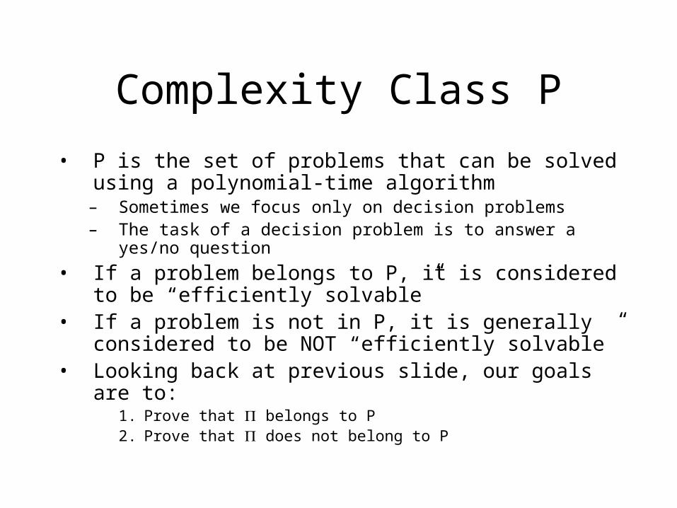
• P is the set of problems that can be solved using a polynomial-time algorithm
– Sometimes we focus only on decision problems– The task of a decision problem is to answer a yes/no question
• If a problem belongs to P, it is considered to be “efficiently solvable”
• If a problem is not in P, it is generally considered to be NOT “efficiently solvable”
• Looking back at previous slide, our goals are to:1. Prove that belongs to P2. Prove that does not belong to P
Hardness Results for Problems
• P: Class of “easy to solve” problems
• Absolute hardness results
• Relative hardness results– Reduction technique
Absolute Hardness Results
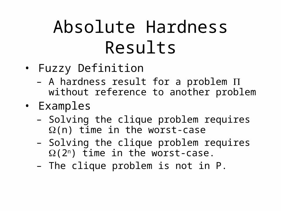
• Fuzzy Definition– A hardness result for a problem without
reference to another problem
• Examples– Solving the clique problem requires (n) time
in the worst-case– Solving the clique problem requires (2n)
time in the worst-case.– The clique problem is not in P.
Proof Techniques
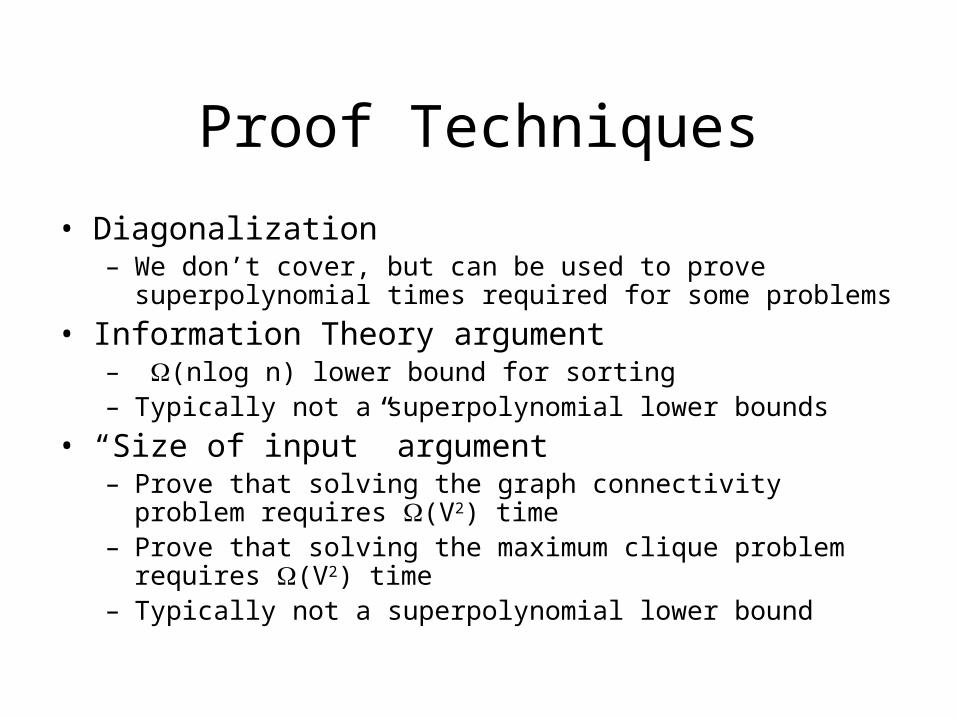
• Diagonalization – We don’t cover, but can be used to prove superpolynomial times
required for some problems
• Information Theory argument – (nlog n) lower bound for sorting– Typically not a superpolynomial lower bounds
• “Size of input” argument– Prove that solving the graph connectivity problem requires (V2) time– Prove that solving the maximum clique problem requires (V2) time– Typically not a superpolynomial lower bound
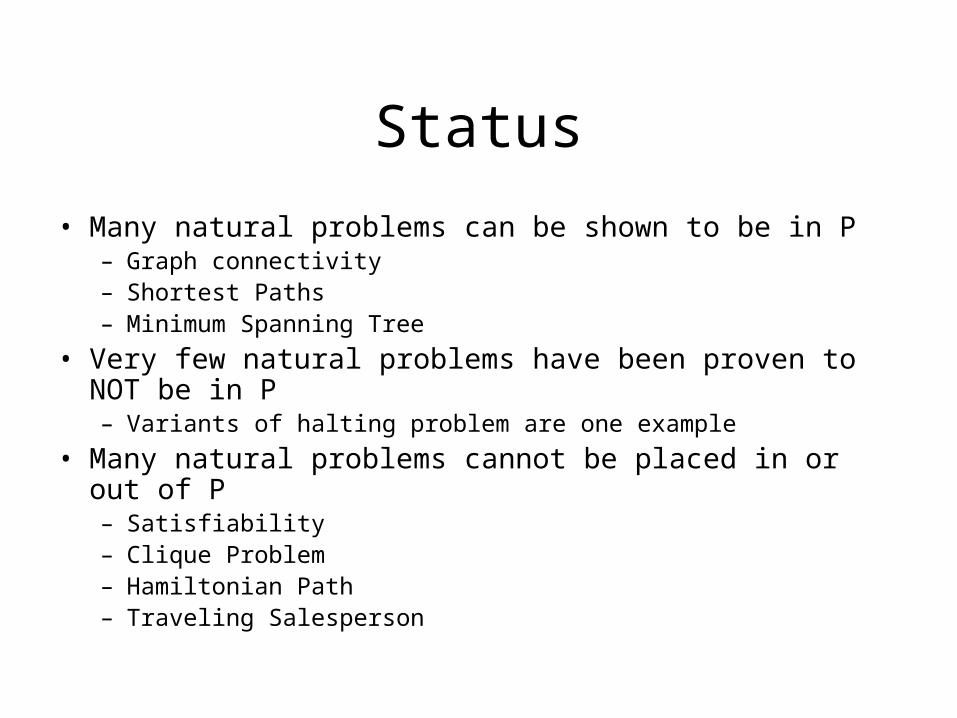
Status
• Many natural problems can be shown to be in P– Graph connectivity– Shortest Paths– Minimum Spanning Tree
• Very few natural problems have been proven to NOT be in P– Variants of halting problem are one example
• Many natural problems cannot be placed in or out of P– Satisfiability– Clique Problem– Hamiltonian Path– Traveling Salesperson
Hardness Results for Problems
• P: Class of “easy to solve” problems
• Absolute hardness results
• Relative hardness results– Reduction technique
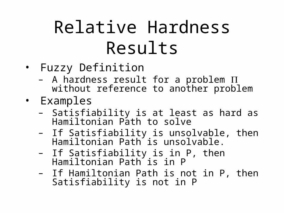
Relative Hardness Results
• Fuzzy Definition– A hardness result for a problem without reference
to another problem• Examples
– Satisfiability is at least as hard as Hamiltonian Path to solve
– If Satisfiability is unsolvable, then Hamiltonian Path is unsolvable.
– If Satisfiability is in P, then Hamiltonian Path is in P– If Hamiltonian Path is not in P, then Satisfiability is
not in P
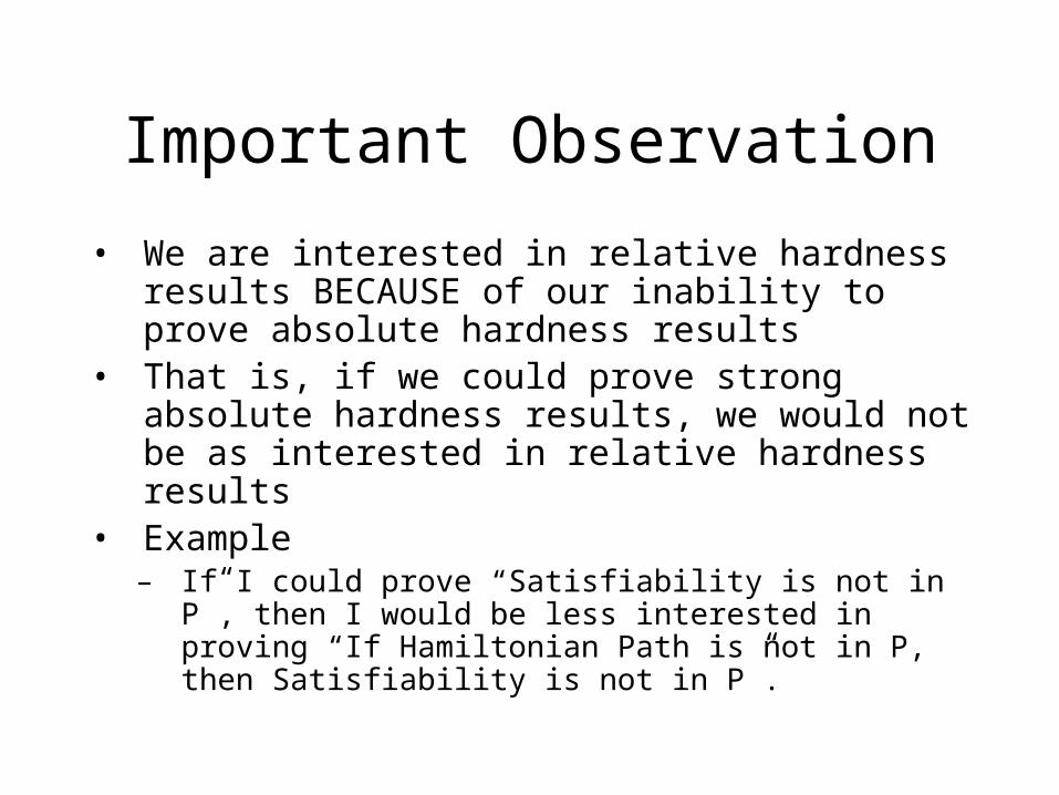
Important Observation
• We are interested in relative hardness results BECAUSE of our inability to prove absolute hardness results
• That is, if we could prove strong absolute hardness results, we would not be as interested in relative hardness results
• Example– If I could prove “Satisfiability is not in P”, then I
would be less interested in proving “If Hamiltonian Path is not in P, then Satisfiability is not in P”.
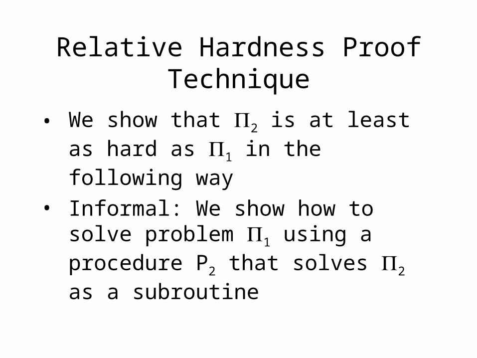
Relative Hardness Proof Technique
• We show that 2 is at least as hard as 1 in the following way
• Informal: We show how to solve problem 1 using a procedure P2 that solves 2 as a subroutine

Examples
• Multiplication and Squaring– square(x) = mult(x,x)
• Proves multiplication is at least as hard as squaring
– mult(x,y) = (square(x+y) – square(x-y))/4• Prove squaring is at least as hard as multiplication
• Assumes that addition, subtraction, and division by 4 can be done with no substantial increase in complexity
• Specific complexity of multiplication may be higher as there are two calls to square, but the difference is polynomially bounded
Hardness Results for Problems
• P: Class of “easy to solve” problems
• Absolute hardness results
• Relative hardness results– Reduction technique
Decision Problems
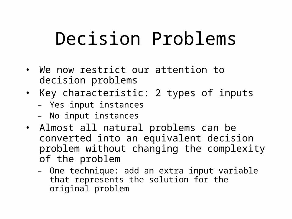
• We now restrict our attention to decision problems
• Key characteristic: 2 types of inputs– Yes input instances– No input instances
• Almost all natural problems can be converted into an equivalent decision problem without changing the complexity of the problem
– One technique: add an extra input variable that represents the solution for the original problem
No loss of complexity
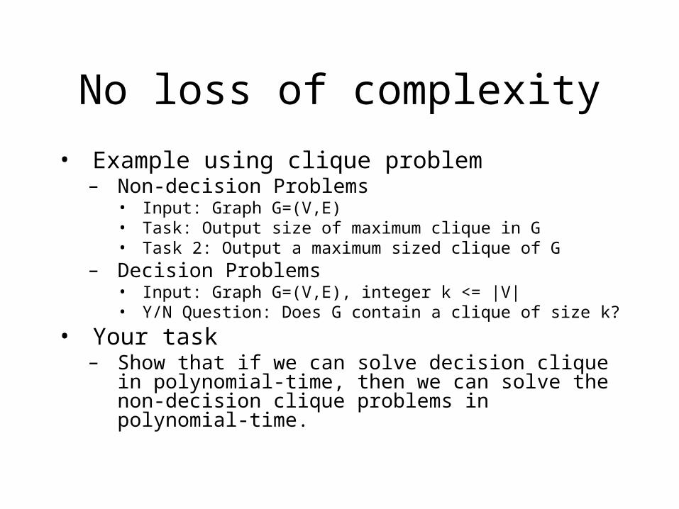
• Example using clique problem– Non-decision Problems
• Input: Graph G=(V,E)• Task: Output size of maximum clique in G• Task 2: Output a maximum sized clique of G
– Decision Problems• Input: Graph G=(V,E), integer k <= |V|• Y/N Question: Does G contain a clique of size k?
• Your task– Show that if we can solve decision clique in
polynomial-time, then we can solve the non-decision clique problems in polynomial-time.
Reduction Technique
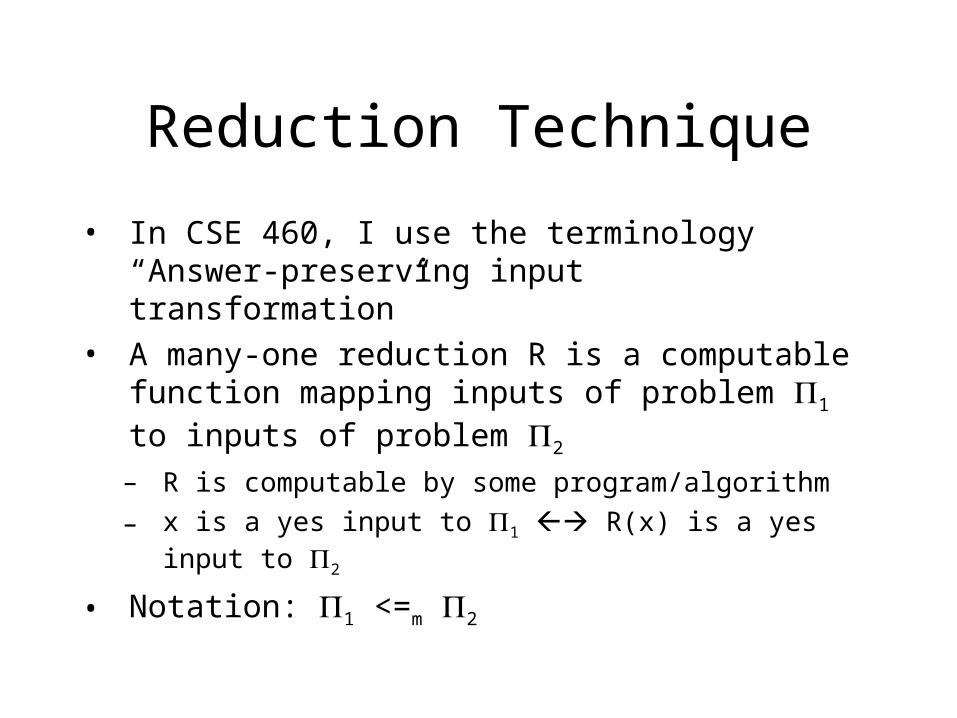
• In CSE 460, I use the terminology “Answer-preserving input transformation”
• A many-one reduction R is a computable function mapping inputs of problem 1 to inputs of problem 2
– R is computable by some program/algorithm
– x is a yes input to 1 R(x) is a yes input to 2
• Notation: 1 <=m 2

Pictoral Representation of Reduction
P1 solves 1
xInput to 1
Yes/NoP2
solves2
Y/NR R(x)
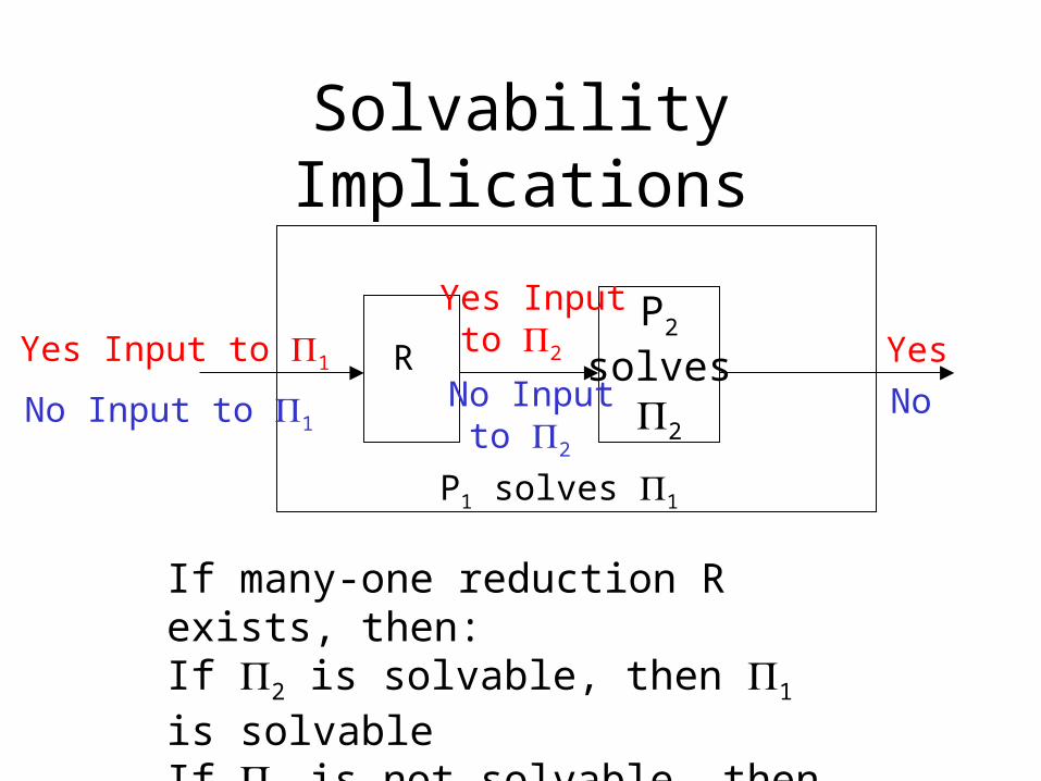
Solvability Implications
P1 solves 1
P2
solves2
R
No Input to 1No Input to 2
Yes Input to 1
Yes Input to 2 Yes
No
If many-one reduction R exists, then:If 2 is solvable, then 1 is solvableIf 1 is not solvable, then 2 is not solvable
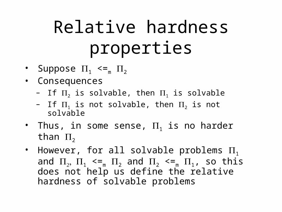
Relative hardness properties
• Suppose 1 <=m 2 • Consequences
– If 2 is solvable, then 1 is solvable– If 1 is not solvable, then 2 is not solvable
• Thus, in some sense, 1 is no harder than 2
• However, for all solvable problems 1 and 1 <=m 2 and 2 <=m 1, so this does not help us define the relative hardness of solvable problems
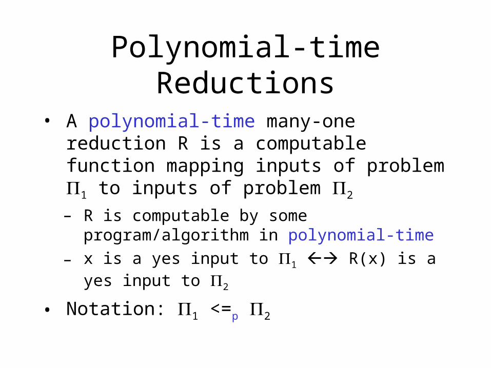
Polynomial-time Reductions
• A polynomial-time many-one reduction R is a computable function mapping inputs of problem 1 to inputs of problem 2
– R is computable by some program/algorithm in polynomial-time
– x is a yes input to 1 R(x) is a yes input to 2
• Notation: 1 <=p 2
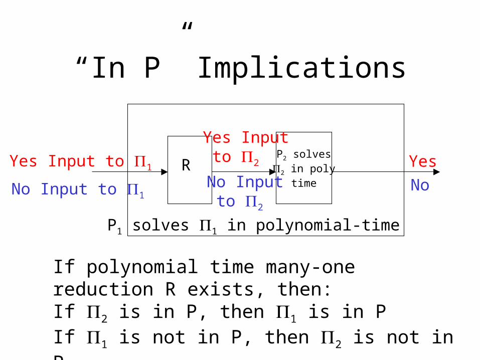
“In P” Implications
P1 solves 1 in polynomial-time
P2 solves2 in poly
time
R
No Input to 1No Input to 2
Yes Input to 1
Yes Input to 2 Yes
No
If polynomial time many-one reduction R exists, then:If 2 is in P, then 1 is in PIf 1 is not in P, then 2 is not in P
Relative hardness properties
• Suppose 1 <=p 2
• Consequences– If 2 is in P, then 1 is in P
– If 1 is not in P, then 2 is not in P
• Thus, in exactly the sense we want, 1 is no harder than 2

Showing 1 <= 2
• For any x input for 1, specify what R(x) will be• Show that R(x) has polynomial size relative to x
– You should show that R runs in polynomial time; I only require the size requirement above
• Show that if x is a yes instance for 1, then R(x) is a yes instance for 2
• Show that if x is a no instance for 1, then R(x) is a no instance for 2
– Often done by showing that if R(x) is a yes instance for 2, then x must have been a yes instance for 1

Example: HP <=p HC
• Hamiltonian Path– Input: Undirected Graph G = (V,E) – Y/N Question: Does G contain a Hamiltonian
Path?
• Hamiltonian Cycle– Input: Undirected Graph G = (V,E)– Y/N Question: Does G contain a Hamiltonian
Cycle?

Specification of R(x)
• Consider any undirected graph G = (V,E) as input x
• R(x) will be a graph G’ = (V’, E’) where– V’ = V union {v} where v is not in V– E’ = E union {(v,w) | w in V}
• Argument that R(x) has polynomial size– We add exactly 1 node and |V| edges.

x is yes R(x) is yes
• Suppose graph G has a Hamiltonian Path• Let this path be v1, v2, …, vn
• We now argue that v1, v2, …, vn, v is a Hamiltonian Cycle in G’
– First, all nodes in V’ are included exactly once above or else v1, v2, …, vn would not be a HP in G
– Since G’ has all the edges that G has, (vi,vi+1) is an edge in E’ for 1 <= i <= n-1
– Finally, since E’ contains edge (v,w) for all w in V, it must be the case that E’ contains edges (vn, v) and (v,v1).

R(x) is yes x is yes
• Suppose graph G’ has a Hamiltonian Cycle
• Let this cycle be v1, v2, …, vn, v
• We now argue that v1, v2, …, vn is a Hamiltonian Path in G
– First, all nodes in V are included exactly once above or else v1, v2, …, vn, v would not be a HC in G’
– Since the only extra edges in E’ compared to E are edges involving node v, it must be the case that E contains edge (vi,vi+1) for 1 <= i <= n-1

Turing Reducibility
• Phil made a suggestion for an alternate reduction.• Given graph G, output (n2) graphs Gv,w = (V,Ev,w) where
– Ev,w = E union {(v,w)} where v,w are nodes in V• This is not a polynomial-time reduction because we are outputting
(n2) graphs.• However, this idea can be used to show that if HC can be solved in
polynomial time, then HP can be solved in polynomial time.– Run each graph Gv,w through our procedure that solves HC. – If HC says yes for any one of these graphs, return yes. – Otherwise return no.
• This more general reduction is often called a Turing reduction.• We allow ourselves to use the procedure that solves HC (or 2) a
polynomial number of times rather than just once.


![1 Tight Hardness Results for Some Approximation Problems [mostly Håstad] Adi Akavia Dana Moshkovitz S. Safra.](https://static.fdocuments.in/doc/165x107/56649d5e5503460f94a3d717/1-tight-hardness-results-for-some-approximation-problems-mostly-hastad-adi.jpg)


![Tight Hardness Results for Some Approximation Problems [mostly Håstad]](https://static.fdocuments.in/doc/165x107/56813d2c550346895da6f162/tight-hardness-results-for-some-approximation-problems-mostly-hastad.jpg)
![1 Tight Hardness Results for Some Approximation Problems [Raz,Håstad,...] Adi Akavia Dana Moshkovitz & Ricky Rosen S. Safra.](https://static.fdocuments.in/doc/165x107/56649d3e5503460f94a16776/1-tight-hardness-results-for-some-approximation-problems-razhastad.jpg)

