HARDNESS AND PENETRATION OF GUTTA PERCHA WHEN …

HARDNESS AND PENETRATION OF GUTTA PERCHA

WHEN EXPOSED TO TWO ENDODONTIC SOLVENTS

EBRAHIM PATEL

A research report submitted to the Faculty of Health Sciences, University of the

Witwatersrand, in partial fulfilment of the requirements for the degree of Master of Science

in Dentistry.

Supervisor:

Professor CP Owen

School of Oral Health Sciences, Faculty of Health Sciences, University of the Witwatersrand,

South Africa

Johannesburg, 2014

ii

DECLARATION

I, Ebrahim Patel, declare that this research report is my own work. It has been submitted for the

degree of Master of Science in Dentistry in the Faculty of Health Sciences at the University of the

Witwatersrand, Parktown, Johannesburg, South Africa. It has not been submitted before for any other

degree or examination at this or any other University.

………………………………………….

This 4th day of July 2014

iii

ABSTRACT

Purpose: Endodontic retreatment requires the removal of the obturation material from the

root canal system. Gutta percha (GP), the most commonly employed obturation material,

requires mechanical instrumentation coupled with a chemical adjunct to facilitate its removal.

Xylene and Eucalyptus oil are recommended as endodontic solvents due to their dissolving

capacity of GP. This study sought to test the changes in the hardness and penetrability of

three types of GP (Conventional, Thermafil® and Guttacore™) when exposed to these

solvents, utilizing distilled water as a control.

Method and materials: Textural analysis was performed to determine the hardness by

testing for rigidity, and the penetrability by testing for deformation energy and resilience.

These properties were tested on 81 GP cones prior to, and following solvent exposure. For

each outcome variable, results were tabulated by group. Between-group differences were

assessed by means of a General Linear Model, with the outcome variable as the dependent

variable and the solvent, GP type and solvent-GP type interaction as the independent

variables.

Results: A significant decrease in rigidity and deformation energy was observed across all

groups. Resilience was observed to decrease with the thermoplastic GP, Thermafil and

Guttacore, but increased with conventional GP. Thermoplastic GP was more amenable to a

reduction in hardness and penetration when compared with Conventional GP. A greater

reduction in the hardness of Thermafil was observed with Eucalyptus oil. Conventional GP

was susceptible to a significant reduction in hardness with both solvents, however its

penetrability may be reduced following exposure to Xylene. Guttacore was significantly

altered by both solvents.

iv

Conclusions: Considering the toxicity profile of Xylene, and the biocompatibility and

antimicrobial effects of Eucalyptol, Eucalyptus oil is recommended for use during endodontic

retreatment.

v

ACKNOWLEDGMENTS

In completion of this work, the author would like to convey his sincerest gratitude and

appreciation to the various individuals that have assisted and guided him towards this goal.

Firstly, to The Almighty, The All-Knowing, without Whom, none one of this would have

been possible.

To my Supervisor and Professor, Peter Owen, for the invaluable role played in the successful

completion of this research report. You not only served as my supervisor, but encouraged and

challenged me throughout my academic programme, never accepting less than my best

efforts. By always expecting perfection, hard work, and commitment, you have instilled in

me qualities which would allow me to excel in life and I thank you for this. Your passion and

dedication to Dentistry and hunger for knowledge is inspirational!

To my co-workers, Dr Saidah Tootla and Dr Megna Gangadin, your valuable feedback and

suggestions helped me improve both my lab experiments and my research in many ways. I

wish you both all the success in your future endeavours.

To my wife and best friend, Rubina Shaikh-Patel, words cannot express my gratitude. For

always believing in me and with your unwavering support, encouragement, patience and

understanding, you provided me with the strength to perform better than I expected.

vi

A special thank you to:

Mr Pradeep Kumar who assisted me with the textural analysis. Thank you for the advice,

direction and training in textural analysis. I will always be grateful to you for easing the

burden of the laboratory work.

To Miss Leigh Spamer who assisted with the acquisition of the several GP cones required in

this study. For going the extra mile to ensure the cones were received on time and for always

being available to offer invaluable support and information.

To Professor Viness Pillay and the Department of Pharmacy. Thank you for assisting me, not

only in the acquisition of materials, but in the use of your facilities, specifically the TA.XT

Plus textural analyser, that was paramount in completing this research.

And finally, to my funders, without whom this research would not have been possible, I

would like to extend my heartfelt gratitude to the FRC grant programme at the Health

Science Research Office, University of the Witwatersrand.

To summarize, over the last few years I ventured far from my comfort-zone, I experienced, I

made mistakes, I learned, I matured…The excitement does not stop here of course, for I still

have a lot to learn…

“The real voyage of discovery consists not in seeking new landscapes, but in having new

eyes.”

- Marcel Proust (French novelist: 1871 - 1922)

vii

TABLE OF CONTENTS

CHAPTER 1 – INTRODUCTION AND LITERATURE REVIEW ........................................................... 1

1.1. Background to the Study ............................................................................................................... 1

1.2. Gutta-Percha in Endodontics ........................................................................................................ 2

1.2.1. Conventional Gutta-Percha ................................................................................................... 4

1.2.2. Thermafil Gutta-Percha ......................................................................................................... 4

1.2.3. Guttacore Gutta-Percha ......................................................................................................... 5

1.3. Endodontic Solvents ..................................................................................................................... 6

1.3.1. Xylene ................................................................................................................................... 6

1.3.2. Eucalyptus Oil ....................................................................................................................... 8

CHAPTER 2 – AIM AND OBJECTIVES ................................................................................................. 10

2.1. Aim ............................................................................................................................................. 11

2.2. Objectives ................................................................................................................................... 11

2.3. Null Hypotheses .......................................................................................................................... 11

CHAPTER 3 – METHOD AND MATERIALS ......................................................................................... 11

3.1. Sample Size Calculation ............................................................................................................. 12

3.2. Method and Materials ................................................................................................................. 12

3.3. Data Analysis .............................................................................................................................. 18

CHAPTER 4 – RESULTS .......................................................................................................................... 18

4.1. Background ................................................................................................................................. 19

4.2. Univariate Data Analysis ............................................................................................................ 20

4.3. Comparison with pilot data ......................................................................................................... 26

4.4. Comparison of within-GP types solvent groups before treatment .............................................. 28

4.5. Comparison of physical properties of GP types before solvent treatment .................................. 33

4.5.1. Rigidity ............................................................................................................................... 33

4.5.2. Deformation energy ............................................................................................................ 35

4.5.3. Resilience ............................................................................................................................ 37

4.6. Comparison of physical properties of GP types after solvent exposure ..................................... 40

4.6.1. Rigidity DIFF ...................................................................................................................... 41

viii

4.6.2. Deformation Energy DIFF .................................................................................................. 43

4.6.3. Resilience DIFF .................................................................................................................. 46

4.7. Comparison of the DIFF results for Xylene and Eucalyptus oil ................................................. 48

CHAPTER 5 – DISCUSSION .................................................................................................................... 50

5.1. Hardness ...................................................................................................................................... 51

5.2. Penetration .................................................................................................................................. 52

CHAPTER 6 – CONCLUSIONS AND RECOMMENDATIONS ............................................................ 56

REFERENCES ........................................................................................................................................... 58

APPENDIX A ............................................................................................................................................. 66

APPENDIX B ............................................................................................................................................. 74

APPENDIX C ............................................................................................................................................. 75

ix

LIST OF FIGURES

Fig. 1.1 Chemical structure of gutta-percha (trans-1,4-polyisoprene) ......................................... 2

Fig. 1.2 Chemical structure of natural rubber (cis-1,4-polyisoprene) ......................................... 3

Fig. 1.3 Amake of conventional GP cones size F3. ..................................................................... 4

Fig. 1.4 Thermafil GP cones size F3. .......................................................................................... 5

Fig. 1.5 GuttaCore GP cones size F3. .......................................................................................... 5

Fig. 1.6 Chemical structure of para-xylene (1,4-dimethylbenzene). ........................................... 7

Fig. 1.7 Chemical structure of Eucalyptol (1,8-Cineole)............................................................. 8

Fig. 3.1 Two eppendorf vials ..................................................................................................... 13

Fig. 3.2 A.The TA.XT plus texture analyser, B. Flat-ended probe above mounting plate

with surface markings for positioning, and C. Probe in position 10mm above

platform ........................................................................................................................ 14

Fig. 3.3 A conventional GP cone positioned using the reference graded markings of the

table, with the probe in position 10mm perpendicularly above. .................................. 15

Fig. 3.4 GP cones seated in an endo stand, prior to batch allocation, demonstrating free

contact of the entire circumference of the cone for solvent exposure. ......................... 16

Fig. 3.5 Typical Force–Distance textural analysis graph illustrating the gradient and area

used to calculate rigidity and deformation energy. ...................................................... 17

Fig. 3.6 Typical Force-Time textural analysis graph illustrating the area used to calculate

resilience. ...................................................................................................................... 17

Fig. 4.1 Histogram plots of rigidity distribution before and after solvent exposure, and

the differences between the two measurements. .......................................................... 24

Fig. 4.2 Run order plotting for rigidity (BEFORE, AFTER and DIFF). ................................... 25

x

Fig. 4.3 Box-and-whiskers plot for rigidity (BEFORE). ........................................................... 29

Fig. 4.4 Box-and-whiskers plot for deformation energy (BEFORE). ....................................... 30

Fig. 4.5 Box-and-whiskers plot for resilience (BEFORE). ....................................................... 31

Fig. 4.6 Box-and-whisker plots for resilience (AFTER and DIFF). .......................................... 32

Fig. 4.7 Box-and-whisker plot of the raw data for rigidity prior to solvent exposure. .............. 34

Fig. 4.8 Least-Squares means plot for rigidity prior to solvent exposure.................................. 35

Fig. 4.9 Box-and-whisker plot of the raw data for deformation energy prior to solvent

exposure........................................................................................................................ 36

Fig. 4.10 Least-Squares means plot for deformation energy prior to solvent exposure. ............. 37

Fig. 4.11 Box-and-whisker plot of the raw data for resilience prior to solvent exposure. .......... 38

Fig. 4.12 Least-Squares means plot for resilience prior to solvent exposure. ............................. 39

Fig. 4.13 Least-Squares means plot for resilience prior to solvent exposure (excluding

C/X data). ..................................................................................................................... 40

Fig. 4.14 Box-and-whisker plot of the raw data for rigidity DIFF. ............................................. 41

Fig. 4.15 Least-Squares means plot for rigidity DIFF following solvent exposure. ................... 42

Fig. 4.16 Box-and-whisker plot of the raw data for deformation energy DIFF following

solvent exposure. .......................................................................................................... 44

Fig. 4.17 Least-Squares means plot for deformation energy DIFF following solvent

exposure........................................................................................................................ 45

Fig. 4.18 Box-and-whisker plot of the raw data for resilience DIFF following solvent

exposure........................................................................................................................ 46

Fig. 4.19 Least-Squares means plot for resilience DIFF following solvent exposure. ................ 47

xi

LIST OF TABLES

Table 3.1 Group allocation of the three types of gutta-percha grouped with the respective

solvents....................................................................................................................... 13

Table 4.1 Univariate statistics for the three dependent variables for Conventional GP. ........... 21

Table 4.2 Univariate statistics for the three dependent variables for Guttacore. ....................... 22

Table 4.3 Univariate statistics for the three dependent variables for Thermafil. ....................... 23

Table 4.4 Univariate statistics comparing the pilot data to the main data set. ........................... 27

Table 4.5 Source table for the dependent variables. .................................................................. 29

Table 4.6 Source table for rigidity prior to solvent exposure. ................................................... 34

Table 4.7 Source table for deformation energy prior to solvent exposure. ................................ 36

Table 4.8 Source table for resilience prior to solvent exposure. ................................................ 38

Table 4.9 Source table for resilience prior to solvent exposure (excluding C/X data). ............. 39

Table 4.10 Source table for rigidity DIFF following solvent exposure. ...................................... 42

Table 4.11 Post hoc tests for Rigidity_DIFF indicating the significant differences in red. ......... 43

Table 4.12 Source table for deformation energy DIFF following solvent exposure. .................. 44

Table 4.13 Post hoc tests for Deformation Energy_DIFF indicating the significant

differences in red. ....................................................................................................... 45

Table 4.14 Source table for resilience DIFF following solvent exposure. ................................... 47

Table 4.15 Post hoc tests for Resilience_DIFF indicating the significant differences in red. .... 48

Table 4.16 Comparison of the DIFF results for Xylene and Eucalyptus oil, indicating the

significant differences in red. ..................................................................................... 49

1

CHAPTER 1

INTRODUCTION AND LITERATURE REVIEW

1.1. Background to the Study

Endodontic therapy is concluded with the filling of the root canal system to provide as perfect

a seal as possible in order to facilitate periapical repair. This is a critical step which requires

three-dimensional filling of the canals (Schilder, 1967; Gutmann et al, 2010). Since its

introduction as a root filling material by Bowman in 1867, gutta-percha (GP) remains the

material of choice for obturation, and has thus been synonymous with endodontic obturation

(Prakash et al, 2005). While satisfying many of the requirements of an ideal obturation

material (plasticity, ease of manipulation, minimal toxicity, radiopacity and ease of removal

with solvents), GP lacks sufficient adhesiveness and rigidity, and easily displaces under

pressure. However, these properties do not overshadow its advantages (Gutmann et al, 2010).

Successful endodontic therapy is dependent on multiple factors, some of which include

adequate disinfection of the root canal system, correct preparation and adequate seal of the

canals and the tooth. However, at times even meticulously performed endodontic therapies

fail, resulting in the need for endodontic retreatment (Whitworth and Boursin, 2000; Martos

et al, 2006).

The main objective of endodontic retreatment requires the removal of the GP filling material

from the canal/s and to regain access to the apical foramen (Tasdemir et al, 2008). Whilst

mechanical instrumentation serves as the primary method of GP removal, many studies have

shown that this alone is insufficient due to the presence of residual GP material in the canal

2

(Hűlsmann and Bluhm, 2004; Ezzie et al, 2006). Therefore, chemical solvents have been

proposed which then serve as an adjunct to mechanical removal (Magalhães et al, 2007). The

solvent softens and partially dissolves the gutta-percha, rendering it more amenable to

removal with hand instruments and thereby decreasing the risk of perforation (Kaplowitz,

1991).

1.2. Gutta-Percha in Endodontics

Gutta-Percha, first used in the Malaysian archipelago, is derived from the malay language as

“Getah” meaning gum, and “Pertja” which refers to the tree (Prakash et al, 2005). GP is a

trans-1,4-polyisoprene (Fig. 1.1). It is derived from Palaquium gutta bail obtained from the

tree family Sapotaceae, by dried coagulated extracts (Gurgel-Filho et al, 2003). Whilst GP

resembles natural rubber in many of its mechanical properties, it is harder, less elastic and

more brittle due to its trans-isomer. This isomer differs from the cis-isomer of natural rubber

(Fig. 1.2) in that it is more linear and crystallizes more easily (Metzger et al, 2011). The

crystalline phase appears in two forms, the Alpha (α) phase and the Beta (β) phase. The

transformation from the β-phase to the α-phase occurs at the endothermic peak between 42oC

and 49oC. The forms differ only in the molecular repeat distance and single carbon-bond

configuration (Schilder et al, 1974).

Fig. 1.1 Chemical structure of gutta-percha (trans-1,4-polyisoprene)

(adapted from Roberts and Caserio, 1979).

3

Fig. 1.2 Chemical structure of natural rubber (cis-1,4-polyisoprene)

(adapted from Roberts and Caserio, 1979).

Conventionally, commercial Gutta Percha cones were composed of inorganic zinc oxide,

barium sulphate, waxes, resins and organic gutta-percha. The percentage composition of

these components differed between manufacturers (Marciano and Michailesco, 1989).

However, Maniglia-Ferreira et al confirmed in 2005 that the absence of barium sulphate is

not unusual in some of the more recent manufacturing forms of GP. Variations in the

proportions of its inorganic components to the gutta-percha would lead to variations in the

brittleness, stiffness, tensile strength and force, and thermal behaviour (Schilder et al, 1974).

Advances in technology have led to the advent of new types of GP. In addition to

conventional GP utilised with cold lateral condensation obturation techniques, thermoplastic

GP as well as the recently launched cross-linked GP have been developed, which permit

warm vertical condensation. However, in 2004 Tsukada et al reported that the techniques

using melted GP alone may not be favourable compared with conventional lateral

condensation, because the melted GP undergoes a large amount of volumetric shrinkage in

the crystalline polymer at phase-transition during setting. This shrinkage hinders the sealing

ability of the GP and thus compromises successful endodontic therapy, although ironically it

may favour retreatment due to greater penetration of the solvent in the potential spaces

created.

4

1.2.1. Conventional Gutta-Percha

Conventional GP (Fig. 1.3) has pure gutta-percha and zinc oxide as its bulk constituents

(Meyer et al, 2006). The percentage contribution of the gutta-percha ranges from 19 - 22,

whereas the zinc oxide ranges from 59 - 79 (Metzger et al, 2011). During endodontic

retreatment, solvents and files contact the surface layer of the coronal GP which enables them

to uniformly soften this layer.

Fig. 1.3 A make of conventional GP cones size F3.

1.2.2. Thermafil Gutta-Percha

Thermafil® (Dentsply, York, USA) (Fig. 1.4) consists of warm α-phase gutta-percha wrapped

around a central polysulfone core. When heated the α-phase gutta-percha becomes pliable

and tacky and will flow when pressure is applied. It has been reported that solvents used

during retreatment (with the exception of chloroform) are able to soften the circumferential

GP only with little/no effect on the core (Ibarrola et al, 1993).

5

Fig. 1.4 Thermafil GP cones size F3.

1.2.3. Guttacore Gutta-Percha

Guttacore™

(Dentsply, York, USA) (Fig. 1.5) has an internal cross-linked gutta-percha core

surrounded by an outer layer of α-phase gutta-percha (Gutmann, 2011). When heated, only

the outer α-phase gutta-percha will flow whilst the inner core remains firm. Thus no

shrinkage of the inner core occurs due to the absence of the transitional phase. According to

the manufacturer, Guttacore is removed more easily than other carrier-based systems.

However, the core behaves unlike gutta-percha in that it does not readily dissolve with

solvents and it is not as amenable to plasticising with heat. During endodontic retreatment,

the solvents coming into contact with the GP will only soften the circumferential α-phase

gutta-percha with no change to the central gutta-percha core (Beasley et al, 2013).

Fig. 1.5 GuttaCore GP cones size F3.

6

1.3. Endodontic Solvents

Advances in endodontic retreatment have also lead to changes in the solvents used to soften

and remove the GP from within the root canal system. Chloroform and Halothane were for

many years the solvents of choice as they were the most effective in dissolving endodontic

sealants (Wilcox, 1995; Ferreira et al, 2001). However, due to their related toxicity and

carcinogenicity, and with the U.S. Food and Drug Administration prohibiting the use of

chloroform, clinicians now seek a suitable alternative (Oyama et al, 1999; Karlović et al,

2001; Azar et al, 2011). Xylol (Xylene) and Eucalyptol are organic solvents which were

introduced as they were not considered potential carcinogens (U.S Department of Health and

Human Service, 1985).

1.3.1. Xylene

Xylene is an aromatic hydrocarbon with the chemical formula of C6H4(CH3)2 (Fig. 1.6) and is

referred to as “dimethyl benzene” because it consists of a six-carbon ring to which two

methyl groups are bound. It is a sweet smelling, colourless liquid occurring naturally in

petroleum, coal and wood tar. Xylene is widely used in medical technology as a solvent (U.S

Department of Health and Human Services, 1993). Dental histological laboratories use

Xylene for tissue processing as its high solvency factor allows for maximum displacement of

alcohol rendering the tissue transparent. Furthermore, it is utilised in staining and cover-

slipping procedures as the Xylene allows for excellent de-waxing and clearing capabilities

that contribute to exceptionally stained slides. Laboratory-grade xylene is composed of m-

xylene (40–65%), p-xylene (20%), o-xylene (20%) and ethyl benzene (6–20%) with traces of

toluene, trimethyl benzene, phenol, thiophene, pyridine and hydrogen sulphide (Kandyala et

al, 2010).

7

Fig. 1.6 Chemical structure of para-xylene (1,4-dimethylbenzene).

The drawback of Xylene, however, is its toxicity to human tissue. This can occur via

inhalation and/or direct contact, with an exposure limit of 100ppm before symptoms such as

nausea and headaches are experienced. In cases of exposure to >200ppm weakness and

vomiting occurs, with consequential loss of consciousness when levels exceed 10,000ppm

(Uchida et al, 1993; Kandyala et al, 2010). However, its restricted use during endodontic

retreatment, coupled with its removal by high-volume suction equipment, limits the exposure

time to the clinician, provided universal infection control barriers such as gloves and masks

are used.

Xylene was established as an efficient solvent during endodontic retreatment as early as the

1980s (Tamse et al, 1986; Wilcox et al, 1987). Its success as a solvent, probably due to

destabilisation of the covalent bonds between the carbon atoms of the gutta-percha, has been

further proven in studies conducted in the 1990s as well as more recent studies in the 2000s

(Kaplowitz, 1990; Hansen et al, 1998; Oyama et al, 2002; Martos et al, 2006; Magalhães et

al, 2007; Rubino et al, 2012).

8

1.3.2. Eucalyptus Oil

Eucalyptus belongs to the Myrtaceae family and comprises 900 species. This native genus

from Australia comprises more than 300 species which contain volatile oils in their leaves.

However, fewer than 20 of these have a content of greater than 70% of 1,8-cineole (Elaissi et

al, 2012). 1,8-cineole (Fig. 1.7), more commonly known as Eucalyptol, is frequently used in

the cosmetic and pharmaceutical industries. It increases the percutaneous penetration of drugs

and may act as a nasal decongestant. It is also used in the treatment of bronchitis, sinusitis

and asthma due to its related anti-inflammatory action which inhibits the production of

tumour necrosis factor alpha (Juergens et al, 1998; Soares et al, 2005). Eucalyptol has also

been demonstrated to be an anti-bacterial and anti-fungal agent (Takarada et al, 2004; Elaissi

et al, 2012).

Fig. 1.7 Chemical structure of Eucalyptol (1,8-Cineole)

(adapted from Mitchell, 1989).

9

Eucalyptol has been used as an endodontic solvent since the 1850s. However, its popularity

was limited by the efficiency of chloroform in that era. When chloroform-induced cytoxicity

and carcinogenicity became a concern, and the U.S Food & Drug Administration banned the

use of chloroform in 1985, clinicians were forced to turn to other volatile and organic

solvents. Eucalyptol gained popularity once again, and even though it proved to be effective

together with other oils such as orange oil, was still not as effective as solvents such as

Xylene (Oyama et al, 2002; Faria-Júnior et al, 2011). However, its favourable toxicity profile

and biocompatibility lead to advocation for its use (Uemara et al, 1997; Tanomaru-Filho et al,

2010). Wourms et al (1990) attributed the reason for the decreased efficiency of Eucalyptol to

the fact that it could not be heated within the root canals: they demonstrated that increasing

the temperature of the solvent to 37oC increases its penetrability. Johann et al (2006)

confirmed in their review that both Xylene and Eucalyptol are acceptable endodontic

solvents, being able to penetrate GP to at least 10mm within 70 seconds.

Eucalyptol is now an accepted alternative to chloroform, whereas Xylene has been described

as a cytotoxic solvent that may even be carcinogenic (Hunter et al, 1991; Hansen et al, 1998;

Schäfer and Zandbiglari, 2002; Magalhães et al, 2007). Additional commercial solvents such

as Endosolv E, Endosolv R and DMS IV are available. However, their function is limited to

dissolving endodontic sealers and thus they have little or no effect on GP.

To date, several authors have investigated the dissolving ability of multiple solvents on

conventional GP and root canal sealants. Their studies quantified the dissolving capacity of a

solvent by measuring the weight of the GP before and after exposure to it. The findings of

these studies either validated or refuted solvents as capable of dissolving GP or sealants.

None sought to test changes in the physical properties of the GP material (Tanomaru-Filho et

10

al, 2010; Faria-Júnior et al, 2011; Mushtaq et al, 2012). Changes in the physical properties

following solvent exposure are important as they can render the material more easily

removable by mechanical instrumentation; conversely, they make retreatment more difficult.

Properties such as hardness and penetrability of the filling material are particularly important

as mechanical files are required to engage the GP in the root canal to allow its removal

Therefore this study sought to measure and compare the hardness and penetrability of GP

after exposure to solvents.

11

CHAPTER 2

AIM AND OBJECTIVES

2.1. Aim

The aim of this study was to test the changes in the hardness and penetrability of three types

of commercial GP used for endodontic obturation when exposed to two types of solvents, and

to deduce whether these changes would benefit the operator during endodontic retreatment.

2.2. Objectives

1. To determine the hardness and penetrability of three types of gutta-percha

(Conventional, thermoplastic Thermafil®

or cross-linked Guttacore™

), where hardness

is inferred by rigidity and penetration by deformation energy and resilience.

2. To determine how the solvents Xylene and Eucalyptus oil will alter these physical

properties relative to a control of distilled water.

3. To determine which manufacturing form of GP will be more resistant to changes in

their physical properties.

2.3. Null Hypotheses

2.3.1 Neither of the solvents would alter the physical properties of GP significantly.

2.3.2 There will be no significant differences between the two solvents.

12

CHAPTER 3

METHOD AND MATERIALS

3.1. Sample Size Calculation

The sample size estimation, performed in G*Power (Buchner et al, 2009), was based on the

combined influence of gutta-percha type (3 types) and solvent type (3 types) on each of the

outcome variables (hardness and penetration). The effect of GP type and solvent type on each

of the outcome variables was determined by a two-factor ANOVA with interaction. Sample

size estimations were based on a significance level of 5%, a power of 80% and the effect

sizes calculated from pilot data. From these data, the following sample sizes were

determined:

Rigidity (9 groups): the sample size was estimated at 36 (4 per group).

Deformation Energy (9 groups): the sample size was estimated at 81 (9 per group)

Resilience (9 groups): the sample size was estimated at 45 (5 per group)

Due to each individual test yielding measurements on all three outcome variables, ultimately

each group had 9 sets of data. Thus 81 cones were required in total

3.2. Method and Materials

The solvents were Xylene BP and Eucalyptus oil BP with distilled water serving as a control.

Three different types of GP were chosen for the study and grouped as per table 2.1:

conventional Protaper® size F3 GP cones, thermoplastic GP Thermafil

® ISO 030 carrier and

13

cross-linked Guttacore™

0.04 size 030. Each GP cone, from the respective GP type, used was

from the same manufacturing batch to eliminate variations in physical properties.

Table 3.1 Group allocation of the three types of gutta-percha grouped with the respective

solvents.

Gutta-percha

Solvents

Xylene Eucalyptus oil Distilled

Water

(control)

Conventional Gutta Percha Group 1a Group 1b Group 1c

Thermoplastic Thermafil®

Group 2a Group 2b Group 2c

Crosslinked Guttacore™

Group 3a Group 3b Group 3c

The GP cones were placed in eppendorf vials (Fig. 3.1) and labelled according to their

specific experimental group and were numbered from 01 – 81. These numbers were then

tabulated on an Excel® spreadsheet and randomly arranged. Each experimental batch

consisted of 27 vials.

Fig. 3.1 Two eppendorf vials

The gutta-percha from each group was texturally analysed using the TA.XT Plus® texture

analyser (Stable Micro Systems, USA, and used with kind permission from the Department

of Pharmacy under the guidance of Prof V Pillay) (Fig. 3.2A).

14

A flat-ended cylindrical probe was chosen which tested each cone against a fixed horizontal

platform with graded markings (Fig 3.2B,C). These markings allowed for reproducible

positioning of the GP cones. Prior to testing, the TA.XT was first calibrated for weight, force

and distance. A force of 10N with a test speed of 5mm.s-1

was chosen for all tests. The

handles of the Thermafil and Guttacore cones prevented the cones sitting flush on the

measurement table and so these were cut off at a level above their respective rubber stops.

A B

C

Fig. 3.2 A.The TA.XT plus texture analyser, B. Flat-ended probe above mounting plate

with surface markings for positioning, and C. Probe in position 10mm above platform.

15

Each cone was analysed prior to solvent exposure for hardness (rigidity) and penetration

(deformation energy and resilience) (Fig. 3.3).

Fig. 3.3 A conventional GP cone positioned using the reference graded markings of the table,

with the probe in position 10mm perpendicularly above.

The GP cones, according to their group allocation, were first seated in an Endo box®

stand

(Dentsply Maillefer, Switzerland). This allowed for a contact-free surface which facilitated

solvent exposure around the entire cone circumference. The endo stand (with the GP cones)

(Fig. 3.4) was then placed in its Endo box allowing for immersion into 160ml of the

corresponding solvent at 24±1°C for 10 minutes, followed by immersion in 160ml of distilled

water for 20 minutes to neutralise the solvent action. The cones were allowed to dry for 24h

at room temperature 24±1°C. The details surrounding each batch including the ambient room

temperature and the temperature of the solvent and distilled water were recorded. These GP

cones were then texturally reanalysed for rigidity, deformation energy and resilience.

16

Fig. 3.4 GP cones seated in an endo stand, prior to batch allocation, demonstrating free

contact of the entire circumference of the cone for solvent exposure.

The software, Exponent®

, linked to this equipment captured data at 200pps and processed the

data into the Force-Distance and Force-Time graphs illustrated in Figures 3.4 and 3.5

respectively. Rigidity is the gradient (1:2) of the curve on a Force-Distance graph and

deformation energy is the area under the curve on a Force-Distance graph (Fig. 3.5). A Force-

Time graph is used to measure resilience: it is the area from the peak of the curve to the end

point (2:3) divided by the area from the beginning of the curve to its peak (1:2), with the

resultant multiplied by 100 (Fig. 3.6).

17

Fig. 3.5 Typical Force–Distance textural analysis graph illustrating the gradient and area used

to calculate rigidity and deformation energy.

Fig. 3.6 Typical Force-Time textural analysis graph illustrating the area used to calculate

resilience.

18

3.3. Data Analysis

The outcome variable for analysis, for each of the three measurements (rigidity, deformation

energy and resilience), is the difference between the post- and pre-solvent exposure

measurements. For each outcome variable, the results were tabulated by group, showing the

mean and standard deviation of the data. Between-group differences were assessed by means

of a General Linear Model (GLM) with the outcome variable as the dependent variable;

independent variables were the solvent, GP type and solvent-GP type interaction; covariates

were room and solvent temperatures. The 5% significance level was employed throughout the

study. Data analysis was carried out using SAS software (SAS Instutute inc. USA).

19

CHAPTER 4

RESULTS

4.1. Background

The properties measured were rigidity, deformation energy and resilience.

There were 9 treatment combinations (3 levels of solvent tested at each of 3 levels of GP

type). Based on a pilot study, a sample size of 9 per treatment combination was used,

resulting in a total of 81 experiments. These were carried out in random order, over a period

of 3 days (27 experiments per day).

Experiments were conducted by measuring each of the three properties on the sample cone

(BEFORE measurement), followed by immersing the sample in the solvent for 10 min at

24±1°C. After rinsing the sample in demineralised water for 20 minutes, and drying at

24±1°C for 24 hours, the three properties were again measured (AFTER measurement).

Since each sample thus acts as its own control, the ultimate measurement of interest for each

property was the difference between the AFTER and BEFORE measurements

(DIFF=AFTER-BEFORE). The AFTER results are attached as Appendix A.

20

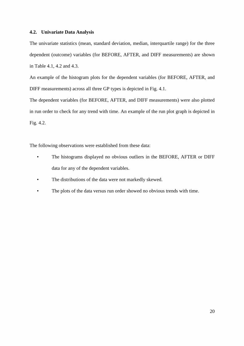
4.2. Univariate Data Analysis

The univariate statistics (mean, standard deviation, median, interquartile range) for the three

dependent (outcome) variables (for BEFORE, AFTER, and DIFF measurements) are shown

in Table 4.1, 4.2 and 4.3.

An example of the histogram plots for the dependent variables (for BEFORE, AFTER, and

DIFF measurements) across all three GP types is depicted in Fig. 4.1.

The dependent variables (for BEFORE, AFTER, and DIFF measurements) were also plotted

in run order to check for any trend with time. An example of the run plot graph is depicted in

Fig. 4.2.

The following observations were established from these data:

• The histograms displayed no obvious outliers in the BEFORE, AFTER or DIFF

data for any of the dependent variables.

• The distributions of the data were not markedly skewed.

• The plots of the data versus run order showed no obvious trends with time.

21

Table 4.1 Univariate statistics for the three dependent variables for Conventional GP.

GP

ty

pe

So

lven

t

n Variable

Mea

n

Sta

nd

ard

Dev

iati

on

95%

Confidence

Limits for

Mean Min

imu

m

Ma

xim

um

Med

ian

Inter-quartile

Range

Co

nv

enti

on

al

Dis

till

ed W

ate

r

9

Rigidity_BEFORE 65.19 2.34 63.39 67.00 61.77 68.26 65.73 63.69 66.92

Rigidity_AFTER 62.17 2.33 60.38 63.96 58.30 65.31 62.81 59.94 63.80

Rigidity_DIFF -3.02 3.10 -5.41 -0.64 -8.62 1.81 -2.97 -3.75 -1.38

Deformation_Energy_

BEFORE 3.93 0.22 3.76 4.10 3.57 4.26 3.95 3.81 4.11

Deformation_Energy_

AFTER 3.78 0.23 3.60 3.96 3.36 4.07 3.83 3.62 3.94

Deformation_Energy_

DIFF -0.15 0.34 -0.41 0.11 -0.79 0.42 -0.17 -0.29 -0.03

Resilience_BEFORE 96.65 1.61 95.41 97.88 94.63 99.95 96.65 95.43 97.41

Resilience_AFTER 94.81 1.83 93.40 96.22 92.24 97.86 94.67 93.57 96.18

Resilience_DIFF -1.84 2.69 -3.90 0.23 -6.77 3.23 -1.67 -2.51 -1.23

Eu

caly

ptu

s O

il

9

Rigidity_BEFORE 62.02 4.21 58.78 65.25 55.66 67.72 60.81 58.66 65.26

Rigidity_AFTER 54.17 2.06 52.59 55.76 52.10 58.87 53.50 52.82 54.69

Rigidity_DIFF -7.84 4.89 -11.60 -4.08 -15.17 -1.31 -8.36 -10.32 -4.66

Deformation_Energy_

BEFORE 3.80 0.24 3.62 3.98 3.50 4.22 3.77 3.67 3.86

Deformation_Energy_

AFTER 3.29 0.16 3.16 3.41 3.07 3.59 3.23 3.20 3.32

Deformation_Energy_

DIFF -0.51 0.35 -0.78 -0.24 -1.03 0.05 -0.61 -0.69 -0.28



Resilience_DIFF 3.02 9.60 -4.36 10.40 -12.42 18.72 1.65 -4.33 9.27

Xy

len

e

9

Rigidity_BEFORE 65.02 2.43 63.15 66.88 60.15 68.35 65.31 64.24 65.84

Rigidity_AFTER 40.56 10.41 32.56 48.57 30.73 57.86 36.89 31.15 46.24

Rigidity_DIFF -24.45 10.88 -32.81 -16.09 -35.01 -5.46 -27.88 -33.96 -19.09

Deformation_Energy_

BEFORE 3.92 0.13 3.82 4.02 3.63 4.13 3.95 3.89 3.95

Deformation_Energy_

AFTER 2.02 0.82 1.38 2.65 1.17 3.28 1.59 1.38 2.52

Deformation_Energy_

DIFF -1.90 0.92 -2.61 -1.20 -2.77 -0.35 -2.48 -2.57 -1.33


Resilience_AFTER 96.28 6.37 91.38 101.1

7 84.60 106.37 96.99 91.98 99.01

Resilience_DIFF 11.55 11.61 2.62 20.47 -16.24 23.57 14.78 8.60 16.03

22

Table 4.2 Univariate statistics for the three dependent variables for Guttacore. G

P t

yp

e

So

lven

t

n Variable

Mea

n

Sta

nd

ard

Dev

iati

on

95%

Confidence

Limits for

Mean Min

imu

m

Ma

xim

um

Med

ian

Inter-quartile

Range

Gu

tta

core

Dis

t W

ate

r

9

Rigidity_BEFORE 90.41 10.67 82.22 98.61 74.45 103.09 92.14 81.81 98.80

Rigidity_AFTER 87.76 8.56 81.17 94.34 73.11 99.28 89.86 82.61 91.69

Rigidity_DIFF -2.66 17.55 -16.15 10.83 -24.54 23.44 -9.53 -13.30 12.90

Deformation_Energy_

BEFORE 5.21 0.92 4.50 5.92 3.92 6.47 5.58 4.47 5.88

Deformation_Energy_

AFTER 5.11 0.66 4.60 5.62 4.13 6.02 5.22 4.60 5.54

Deformation_Energy_

DIFF -0.10 1.42 -1.19 0.99 -1.76 1.93 -0.93 -1.04 1.30



Resilience_DIFF -2.67 3.10 -5.06 -0.29 -7.90 2.92 -3.18 -4.08 -1.87

Eu

caly

ptu

s O

il

9

Rigidity_BEFORE 90.17 9.22 83.08 97.26 75.48 102.25 92.57 82.16 96.48

Rigidity_AFTER 42.25 8.90 35.41 49.09 31.66 57.49 38.69 36.89 43.39

Rigidity_DIFF -47.92 13.52 -58.31 -37.53 -70.59 -31.20 -47.06 -57.91 -36.92

Deformation_Energy_

BEFORE 5.28 0.83 4.64 5.92 3.97 6.38 5.40 4.72 5.90

Deformation_Energy_

AFTER 2.05 0.37 1.76 2.33 1.75 2.69 1.84 1.80 2.10

Deformation_Energy_

DIFF -3.24 0.95 -3.96 -2.51 -4.54 -1.86 -2.92 -3.92 -2.52



Resilience_DIFF -1.25 9.44 -8.50 6.01 -12.72 15.65 -2.72 -8.34 4.91

Xy

len

e

9

Rigidity_BEFORE 85.83 12.70 76.07 95.60 62.42 99.34 90.67 80.29 92.45

Rigidity_AFTER 34.73 4.64 31.17 38.30 27.53 40.22 34.75 32.20 39.86

Rigidity_DIFF -51.10 14.33 -62.11 -40.09 -66.17 -22.43 -56.34 -61.13 -45.55

Deformation_Energy_

BEFORE 4.53 0.82 3.90 5.17 3.22 5.46 4.76 3.78 5.19

Deformation_Energy_

AFTER 1.58 0.43 1.25 1.91 0.97 2.06 1.85 1.23 1.91

Deformation_Energy_

DIFF -2.95 0.92 -3.66 -2.24 -3.79 -1.26 -3.31 -3.59 -2.55



Resilience_DIFF -10.02 6.40 -14.94 -5.10 -24.26 -3.64 -7.39 -9.15 -7.07

23

Table 4.3 Univariate statistics for the three dependent variables for Thermafil. G

P t

yp

e

So

lven

t

n Variable

Mea

n

Sta

nd

ard

Dev

iati

on

95% Confidence

Limits for Mean

Min

imu

m

Ma

xim

um

Med

ian

Inter-quartile

Range

Th

erm

afi

l

Dis

till

ed W

ate

r

9

Rigidity_BEFORE 89.90 13.92 79.20 100.60 70.24 107.08 86.60 82.54 102.78

Rigidity_AFTER 90.91 7.06 85.49 96.34 80.26 103.34 92.82 85.34 94.61

Rigidity_DIFF 1.01 12.05 -8.26 10.27 -20.74 14.52 5.93 -6.62 8.01

Deformation_Energy_

BEFORE 5.29 1.14 4.42 6.17 3.85 6.71 5.03 4.41 6.38

Deformation_Energy_

AFTER 5.37 0.61 4.90 5.84 4.53 6.53 5.41 4.86 5.67

Deformation_Energy_

DIFF 0.08 1.09 -0.76 0.91 -1.79 1.28 0.64 -0.71 0.78



Resilience_DIFF -0.63 4.05 -3.75 2.48 -8.48 4.06 1.01 -3.62 2.11

Eu

caly

ptu

s O

il

9

Rigidity_BEFORE 91.38 9.93 83.75 99.02 71.53 100.99 95.57 84.96 99.28

Rigidity_AFTER 42.23 10.42 34.22 50.24 29.55 56.07 36.44 35.38 50.68

Rigidity_DIFF -49.15 14.93 -60.63 -37.68 -71.44 -26.24 -49.36 -59.54 -41.29

Deformation_Energy_

BEFORE 5.39 0.80 4.78 6.00 3.82 6.35 5.50 5.01 5.94

Deformation_Energy_

AFTER 2.25 0.54 1.83 2.67 1.62 3.02 2.13 1.81 2.65

Deformation_Energy_

DIFF -3.14 0.90 -3.83 -2.44 -4.22 -1.78 -3.14 -3.89 -2.51



Resilience_DIFF -2.12 7.22 -7.68 3.43 -11.95 10.07 -4.02 -6.26 1.08

Xy

len

e

9

Rigidity_BEFORE 91.42 8.33 85.02 97.83 81.12 101.64 90.36 84.97 99.03

Rigidity_AFTER 59.94 15.50 48.03 71.85 39.53 81.50 55.99 48.68 72.75

Rigidity_DIFF -31.48 13.81 -42.09 -20.86 -58.04 -14.52 -28.89 -34.02 -22.82

Deformation_Energy_

BEFORE 5.82 0.42 5.50 6.14 4.84 6.35 5.81 5.77 6.02

Deformation_Energy_

AFTER 2.60 1.31 1.60 3.61 1.04 4.36 2.01 1.71 3.70

Deformation_Energy_

DIFF -3.22 1.35 -4.25 -2.18 -4.73 -1.16 -3.72 -4.32 -2.31



Resilience_DIFF 1.02 5.69 -3.36 5.39 -5.69 11.85 -0.33 -2.79 2.69

24

Fig. 4.1 Histogram plots of rigidity distribution before and after solvent exposure, and the

differences between the two measurements.

25

Fig. 4.2 Run order plotting for rigidity (BEFORE, AFTER and DIFF).

26

4.3. Comparison with pilot data

The results of the treatments which corresponded between the pilot and main studies (i.e. for

Xylene and the three GP types) were compared using the Wilcoxon rank sum test (this is the

non-parametric equivalent of the independent samples t-test and was used here due to the

small sample size of the pilot study group). The results are shown in Table 4.4. To ensure

that the pilot and main studies were comparable, there should be no significant differences

noted between the two studies.

Observations deduced from Table 4.4 are as follows:

• The rigidity results (BEFORE, AFTER, and DIFF) were not significantly different

between the pilot and main studies – this is as expected.

• The deformation energy results were completely different between the pilot and main

studies:

o Across the three GP types, the BEFORE values were approximately 4-7 times

higher in the main study than in the pilot study. The AFTER values were not

significantly different (the difference for Thermafil was marginal). Thus the DIFF

values were significantly different: in the pilot study, deformation energy

increased from BEFORE to AFTER, while it decreased in the main study.

• The Resilience results were completely different between the pilot and main studies:

o Across the three GP types, the BEFORE values were approximately 3 times

higher in the main study than in the pilot study, while the AFTER values were 4-5

times higher in the main study than in the pilot study The DIFF values were not

significantly different between the two studies.

27

Table 4.4 Univariate statistics comparing the pilot data to the main data set.

So

lven

t

Variable

Pilot study Main study p-value for

H0: no

significant

difference

between

means

Ra

tio

of

mea

ns:

Ma

in/P

ilo

t

n

Mea

n

Sta

nd

ard

Dev

iati

on

95% Confidence

Limits for Mean n

Mea

n

Sta

nd

ard

Dev

iati

on

95%

Confidence

Limits for

Mean

Xy

len

e –

Co

nv

enti

on

al

GP

Rigidity_BEFORE

4

64.02 2.62 59.86 68.18

9

65.02 2.43 63.15 66.88 0.88 1.0

Rigidity_AFTER 32.40 3.00 27.63 37.17 40.56 10.41 32.56 48.57 0.24 1.3

Rigidity_DIFF -31.62 3.50 -37.19 -26.05 -24.45 10.88 -32.81 -16.09 0.27 0.8

Deformation_Energy_

BEFORE 0.95 0.01 0.94 0.96 3.92 0.13 3.82 4.02 0.019 4.1

Deformation_Energy_

AFTER 1.31 0.14 1.08 1.53 2.02 0.82 1.38 2.65 0.13 1.5

Deformation_Energy_

DIFF 0.36 0.14 0.13 0.58 -1.90 0.92 -2.61 -1.20 0.019 -5.3

Resilience_BEFORE 22.65 0.55 21.77 23.52 84.73 6.10 80.04 89.42 0.019 3.7

Resilience_AFTER 18.57 2.48 14.62 22.51 96.28 6.37 91.38

101.1

7 0.019 5.2

Resilience_DIFF -4.08 1.93 -7.16 -1.00 11.55 11.61 2.62 20.47 0.059 -2.8

Xy

len

e -

Gu

tta

Co

re

Rigidity_BEFORE

4

96.59 15.75 71.54 121.65

9

85.83 12.70 76.07 95.60 0.50 0.9

Rigidity_AFTER 37.00 3.57 31.32 42.68 34.73 4.64 31.17 38.30 0.37 0.9

Rigidity_DIFF -59.60 14.57 -82.79 -36.40 -51.10 14.33 -62.11 -40.09 0.45 0.9

Deformation_Energy_

BEFORE 0.76 0.02 0.72 0.79 4.53 0.82 3.90 5.17 0.019 6.0

Deformation_Energy_

AFTER 1.15 0.18 0.86 1.43 1.58 0.43 1.25 1.91 0.21 1.4

Deformation_Energy_

DIFF 0.39 0.17 0.12 0.66 -2.95 0.92 -3.66 -2.24 0.019 -7.6


Resilience_AFTER 19.98 2.61 15.83 24.13 83.84 6.44 78.89 88.79 0.019 4.2

Resilience_DIFF -7.46 2.29 -11.10 -3.82 -10.02 6.40 -14.94 -5.10 0.88 1.3

Xy

len

e -

Th

erm

afi

l

Rigidity_BEFORE

4

84.74 4.13 78.18 91.31

9

91.42 8.33 85.02 97.83 0.21 1.1

Rigidity_AFTER 49.76 5.34 41.26 58.26 59.94 15.50 48.03 71.85 0.30 1.2

Rigidity_DIFF -34.98 9.11 -49.49 -20.48 -31.48 13.81 -42.09 -20.86 0.50 0.9

Deformation_Energy_

BEFORE 0.78 0.03 0.72 0.83 5.82 0.42 5.50 6.14 0.019 7.5

Deformation_Energy_

AFTER 1.01 0.07 0.90 1.12 2.60 1.31 1.60 3.61 0.045 2.6

Deformation_Energy_

DIFF 0.24 0.08 0.10 0.37 -3.22 1.35 -4.25 -2.18 0.019 -13.7


Resilience_AFTER 23.49 1.38 21.30 25.68 92.26 6.73 87.08 97.43 0.019 3.9

Resilience_DIFF -3.58 1.74 -6.34 -0.81 1.02 5.69 -3.36 5.39 0.12 -0.3

28

It was subsequently established that the test probe speed in the pilot data had been set at

0.5mm.s-1

, whereas in the main study it was set as 5mm.s-1

. Changes in probe speed affect the

contact time of the probe on material constituents, and thus change the resultant graph plot.

Hence, any increase or decrease in probe speed would ultimately alter the resultant values for

any parameter (Klatzky et al, 2003). However, of importance is the DIFF data which indicate

solvent efficiency. For that reason, even with differing BEFORE and AFTER data, the DIFF

values were not significantly different and therefore valid.

4.4. Comparison of within-GP types solvent groups before treatment

In order to validate the use of the DIFF variables to evaluate the effect of solvent treatment,

randomisation was employed to ensure that there were no significant differences in the

BEFORE measurements between the three groups, within each GP type, assigned to each of

the three solvents.

A general linear model with main effect for GP type, solvent (nested in GP type), and

experiment day as a blocking variable, was used to model each of the BEFORE dependent

variables in turn. The variable transformations described in the previous section were

retained; the solvent effect should be non-significant. The source table is shown in Table

4.5, with the box-and-whisker plots illustrating the data shown in Fig. 4.3 and 4.4.

29

Table 4.5 Source table for the dependent variables.

Rigidity_BEFORE (inverse square root transformation)

Source Degrees of

freedom Type 3 Sum of Squares Mean Square F p

GP_type 2 0.00602 0.00301 97.98 <0.0001

Solvent(GP_type) 6 0.000072 0.000012 0.39 0.88

Date 2 0.000053 0.000027 0.87 0.42

Deformation Energy_BEFORE (inverse square root transformation)

GP_type 2 0.0752 0.0376 34.25 <0.0001

Solvent(GP_type) 6 0.0081 0.0013 1.22 0.31

Date 2 0.0008 0.0004 0.37 0.69

Resilience_BEFORE

GP_type 2 234.94 117.47 8.24 0.0006

Solvent(GP_type) 6 822.49 137.08 9.61 <0.0001

Date 2 19.06 9.53 0.67 0.52

Fig. 4.3 Box-and-whiskers plot for rigidity (BEFORE).

30

Fig. 4.4 Box-and-whiskers plot for deformation energy (BEFORE).

For rigidity and deformation energy, only the GP type main effect was significant

(p<0.0001), and the solvent effect was confirmed as non-significant. For resilience however,

the main effect of solvent (p = 0.0006) as well as the ‘Solvent x GP type’ interaction

(p<0.0001), were highly significant. Post-hoc tests showed that the Conventional/Xylene

(C/X) group had significantly lower resilience than the Conventional/Eucalyptus Oil (C/EO)

and Conventional/Distilled water (C/DW) groups. This is illustrated in the box-and-whisker

plot in Fig. 4.5.

31

Fig. 4.5 Box-and-whiskers plot for resilience (BEFORE).

The AFTER results for C/X are roughly in line with those for the other solvents for the

conventional groups. However when DIFF was calculated, C/X was the only one of the 9

treatment groups to display a significant increase in resilience after solvent treatment, against

expectations (Fig. 4.6). The reason for the discrepancy remains unclear. Furthermore, with a

lack of comparative data in the literature, it is difficult to establish whether this finding is

related to experimental error, or is in fact valid. Hence, the resilience data for C/X were

treated with caution.

32

Fig. 4.6 Box-and-whisker plots for resilience (AFTER and DIFF).

33

4.5. Comparison of physical properties of GP types before solvent treatment

Differences in the three physical properties of the three GP types before solvent treatment

were assessed by combining the BEFORE results for the 27 experiments conducted for each

GP type. A general linear model with GP type as main effect and experiment day as blocking

variable was used to model each of the BEFORE dependent variables in turn. (The use of

room, solvent, and desiccator temperatures as covariates was also considered, however kept

constant throughout the study.) Post-hoc tests were conducted using the Tukey-Kramer test.

Effect sizes were calculated using Cohen’s d, which were interpreted as follows:

0.80 and above large effect

0.50 to 0.79 moderate effect

0.20 to 0.39 small effect

below 0.20 near zero effect

4.5.1. Rigidity

A box-and-whisker plot of the raw data, by GP type, is shown in Fig. 4.7. The variance of the

Rigidity_BEFORE increased with its mean; a variance-stabilising transformation was

required for the general linear model, although the conclusions from the raw and transformed

data were the same. An inverse square root transformation of the Rigidity_BEFORE data was

used.

34

Fig. 4.7 Box-and-whisker plot of the raw data for rigidity prior to solvent exposure.

One of the tests (experiment 11) was excluded as an outlier, based on model diagnostics. The

overall model was significant: F(4,75)=57.9; p<0.0001. The source table in Table 4.6 shows

the main effect of GP type to be significant (p<0.0001) and the blocking effect of date not

significant, as was expected.

Table 4.6 Source table for rigidity prior to solvent exposure.

Source Degrees of freedom Type 3 Sum of Squares Mean Square F p

GP_type 2 0.006069 0.003035 103.87 <.0001

Date 2 0.000059 0.000030 1.01 0.37

Post-hoc tests indicated that the mean rigidity (before solvent treatment) of the conventional

GP was significantly lower than that of the other two materials (p<0.001). The Least-Squares

(LS) means plot is shown in Fig. 4.8. The error bars denote the 95% confidence limits for the

35

mean. Least Squares means are the means estimated from the model, over balanced values of

the other covariates in the model.

Fig. 4.8 Least-Squares means plot for rigidity prior to solvent exposure.

Conventional GP had a mean (standard deviation) rigidity of 64.1 (3.3), compared to the

rigidity for Guttacore of 89.8 (9.5) and that for Thermafil of 90.9 (10.6). The effect sizes

were both large (Cohen’s d=3.7 and 3.6 for Conventional vs. Guttacore and Thermafil,

respectively).

4.5.2. Deformation energy

A box-and-whisker plot of the raw data, by GP type, is shown in Fig. 4.9. As with Rigidity,

the variance of the Deformation Energy_BEFORE increased with its mean, and once again a

variance-stabilising inverse square root transformation was required.

0

10

20

30

40

50

60

70

80

90

100

Conventional Guttacore Thermafil

Rig

idit

y_B

EFO

RE:

LS

-Me

ans

Gutta-Percha type

36

The overall model was significant: F(4,76)=20.1; p<0.0001. The source table is shown in

Table 4.7 below and, as with rigidity, the blocking effect of date was not significant.

Fig. 4.9 Box-and-whisker plot of the raw data for deformation energy prior to solvent

exposure.

Table 4.7 Source table for deformation energy prior to solvent exposure.


GP_type 2 0.072 0.036 32.20 <.0001

Date 2 0.0038 0.0019 1.68 0.19

Post-hoc tests indicated that the mean deformation energy (before solvent treatment) of the

Conventional GP was significantly lower than that of the other two materials (p<0.001). The

Least-Squares means plot is shown in Fig. 4.10.

37

Fig. 4.10 Least-Squares means plot for deformation energy prior to solvent exposure.

Conventional GP had a mean (SD) deformation energy of 3.88 (0.20), compared to the

deformation energy for Guttacore of 5.01 (0.90) and that for Thermafil of 5.50 (0.84). The

effect sizes were both large (Cohen’s d=1.8 and 2.7 for Conventional vs. Guttacore and

Thermafil, respectively).

4.5.3. Resilience

A box-and-whisker plot of the raw data, by GP type, is shown in Fig. 4.11. In contrast to

rigidity and deformation energy, the variance did not increase with its mean, and thus a

variance-stabilising inverse square root transformation was not required.

0

1

2

3

4

5

6


De

form

atio

n E

ne

rgy_

BEF

OR

E:

LS

-Me

ans

Gutta-Percha type

38

Fig. 4.11 Box-and-whisker plot of the raw data for resilience prior to solvent exposure.

Experiment 30 was excluded as an outlier, based on model diagnostics. The overall model

was significant: F(4,75) = 2.69; p = 0.038. The source table is shown in Table 4.8 below:

Table 4.8 Source table for resilience prior to solvent exposure.


GP_type 2 190.5 95.2 3.77 0.028

Date 2 80.6 40.3 1.60 0.21

Post-hoc tests indicated that the mean resilience (before solvent treatment) of the

Conventional GP was significantly lower than that of the Guttacore (only) (p=0.021). The

Least-Squares means plot is shown in Fig. 4.12.

39

Fig. 4.12 Least-Squares means plot for resilience prior to solvent exposure.

Conventional GP had a mean (SD) resilience of 90.7 (7.4), compared to the resilience for

Guttacore of 94.5 (3.7) and that for Thermafil of 92.6 (3.2). The effect size for the significant

difference (Conventional vs. Guttacore) was moderate (Cohen’s d=0.67).

Exclusion of C/X data :

Repeating the above analysis for resilience, but excluding the C/X data (n=9), and again

excluding experiment 30 as an outlier, the overall model was not significant: F(4,66)=0.92;

p=0.46. The source table is shown in Table 4.9.

Table 4.9 Source table for resilience prior to solvent exposure (excluding C/X data).


GP_type 2 41.31 20.65 1.17 0.32

Date 2 14.67 7.33 0.41 0.66

0

10

20

30

40

50

60

70

80

90

100


Re

silie

nce

_BEF

OR

E:

LS

-Me

ans

Gutta-Percha type

40

Thus, there was no significant difference in the resilience of the difference GP types before

solvent treatment. The Least-Squares means plot is shown in Fig. 4.13 below.

Fig. 4.13 Least-Squares means plot for resilience prior to solvent exposure (excluding C/X

data).

Thus conclusions drawn across the three types of GP, prior to solvent exposure, were that:

• Conventional GP had significantly lower rigidity and deformation energy than

both Guttacore and Thermafil.

• Conventional GP had significantly lower resilience than Guttacore when all the

data were used. However, excluding the C/X group data there was no significant

difference in the resilience of the different GP types before solvent treatment.

4.6. Comparison of physical properties of GP types after solvent exposure

The effects of the treatments on the DIFF variables for each of the three dependent variables

was assessed using a general liner model with main effects for solvent and GP type, a two-

factor interaction between solvent and GP type, and experiment day as the blocking variable.

0

10

20

30

40

50

60

70

80

90

100


Re

silie

nce

_BEF

OR

E:

LS

-Me

ans

Gutta-Percha type

41

As mentioned previously, the use of room and solvent temperatures as covariates was also

considered, however these remained constant throughout the study. Post-hoc tests were

conducted using the Tukey-Kramer test. Effect sizes were calculated using Cohen’s d

(interpreted as above).

4.6.1. Rigidity DIFF

A box-and-whisker plot of the raw data, by GP type and solvent, is shown in Fig. 4.14.

Fig. 4.14 Box-and-whisker plot of the raw data for rigidity DIFF.

The mean DIFFs were zero or negative indicating that the rigidity remained unchanged or

decreased after solvent treatment. The overall model was significant: F(10,70)=21.3;

p<0.0001, as were the main effects of GP type. The source table is shown in Table 4.10.

42

Table 4.10 Source table for rigidity DIFF following solvent exposure.


GP_type 2 6397.08 3198.54 20.03 <.0001

Solvent 2 20006.91 10003.46 62.65 <.0001

GP_type*Solvent 4 6413.38 1603.34 10.04 <.0001

Date 2 78.22 39.11 0.24 0.78

The two-factor interaction for Least-Squares means plot is shown in Fig. 4.15.

Fig. 4.15 Least-Squares means plot for rigidity DIFF following solvent exposure.

Post-hoc tests indicated significant differences between interactions as per Table 4.11.

-70

-60

-50

-40

-30

-20

-10

0

10

Dist Water Eucalyptus Oil Xylene

Rig

idit

y_D

IFF:

LS-

Me

an

Solvent

Conventional

Guttacore

Thermafil

43

Table 4.11 Post hoc tests for Rigidity_DIFF indicating the significant differences in red.

Least Squares Means for effect GP_type * Solvent

Pr > |t| for H0: LSMean(i)=LSMean(j)

Dependent Variable: Rigidity_DIFF

i/j C / DW C / EO C / Xyl G / DW G / EO G / Xyl T / DW T / EO T / Xyl

C / DW

0.998 0.037 1.000 <.0001 <.0001 0.996 <.0001 0.003

C / EO 0.998

0.175 0.983 <.0001 <.0001 0.826 <.0001 0.015

C / Xyl 0.037 0.175

0.012 0.008 0.001 0.002 0.003 0.980

G / DW 1.000 0.983 0.012

<.0001 <.0001 1.000 <.0001 0.000

G / EO <.0001 <.0001 0.008 <.0001

0.999 <.0001 1.000 0.123

G / Xyl <.0001 <.0001 0.001 <.0001 0.999

<.0001 1.000 0.038

T / DW 0.996 0.826 0.002 1.000 <.0001 <.0001

<.0001 <.0001

T / EO <.0001 <.0001 0.003 <.0001 1.000 1.000 <.0001

0.075

T / Xyl 0.003 0.015 0.980 0.000 0.123 0.038 <.0001 0.075

C:Conventional; G: Guttacore; T: Thermafil; Xyl: Xylene; EO: Eucalyptus Oil; DW: Distilled Water

4.6.2. Deformation Energy DIFF

A box-and-whisker plot of the raw data, by GP type and solvent, is shown in Fig. 4.16. As

with Rigidity, the mean DIFFs were zero or negative, i.e. the deformation energy remained

unchanged or decreased after solvent treatment.

44

Fig. 4.16 Box-and-whisker plot of the raw data for deformation energy DIFF following

solvent exposure.

The overall model was significant: F(10,70)=16.4; p<0.0001, as were the main effects of GP

type and solvent, as well as their interaction. The source table is shown in Table 4.12.

Table 4.12 Source table for deformation energy DIFF following solvent exposure.


GP_type 2 25.20 12.60 12.83 <.0001

Solvent 2 104.22 52.11 53.05 <.0001

GP_type*Solvent 4 21.88 5.47 5.57 0.0006

Date 2 0.36 0.18 0.18 0.83

The two-factor interaction for the Least-Squares means plot is shown in Fig. 4.17.

45

-5

-4

-3

-2

-1

0

1


De

form

atio

n E

ne

rgy_

DIF

F: L

S-M

ean

Solvent

Conventional

Guttacore

Thermafil

Fig. 4.17 Least-Squares means plot for deformation energy DIFF following solvent exposure.


Table 4.13 Post hoc tests for Deformation Energy_DIFF indicating the significant differences

in red.


Least Squares Means for effect GP_type*Solvent


Dependent Variable: Deformation Energy_DIFF


C / DW

0.997 0.012 1.000 <.0001 <.0001 1.000 <.0001 <.0001

C / EO 0.997

0.082 0.996 <.0001 <.0001 0.957 <.0001 <.0001

C / Xyl 0.012 0.082

0.008 0.224 0.490 0.002 0.254 0.192

G / DW 1.000 0.996 0.008

<.0001 <.0001 1.000 <.0001 <.0001

G / EO <.0001 <.0001 0.224 <.0001

1.000 <.0001 1.000 1.000

G / Xyl <.0001 <.0001 0.490 <.0001 1.000

<.0001 1.000 1.000

T / DW 1.000 0.957 0.002 1.000 <.0001 <.0001

<.0001 <.0001

T / EO <.0001 <.0001 0.254 <.0001 1.000 1.000 <.0001

1.000

T / Xyl <.0001 <.0001 0.192 <.0001 1.000 1.000 <.0001 1.000

46

The following were observed focusing on the DIFF per material type:

C/DW > C/X (Cohen’s d=2.7)

G/DW > G/X, G/EO (Cohen’s d=2.5 and 2.6 respectively)

T/DW > T/X, T/EO (Cohen’s d = 2.9 and 3.4 respectively).

All the effect sizes are classified as ‘large’.

4.6.3. Resilience DIFF

The data obtained for resilience were interpreted with caution, given the unexpected results

obtained for Conventional GP/Xylene (C/X) group BEFORE solvent treatment. A box-and-

whisker plot of the raw data, by GP type and solvent, is shown in Fig. 4.18.

Fig. 4.18 Box-and-whisker plot of the raw data for resilience DIFF following solvent

exposure.

47

The mean DIFFs were zero or negative, i.e. the resilience remained unchanged or decreased

after solvent treatment except for C/X, where the resilience increased after solvent treatment

due to the values for Resilience_BEFORE for this group. Experiment 2 was excluded as an

outlier based on model diagnostics. The overall model was significant: F(10,69)=7.1;

p<0.0001, as were the main effect of GP type, as well as the ‘GP type x Solvent’ interaction.

The source table is shown in Table 4.14:

Table 4.14 Source table for resilience DIFF following solvent exposure.


GP_type 2 1320.92 660.46 15.76 <.0001

Solvent 2 181.59 90.80 2.17 0.12

GP_type*Solvent 4 1475.92 368.98 8.80 <.0001

Date 2 37.96 18.98 0.45 0.64

The two-factor interaction for the Least-Squares means plot is shown in Fig 4.19.

Fig. 4.19 Least-Squares means plot for resilience DIFF following solvent exposure.

-20

-15

-10

-5

0

5

10

15

20

25


Re

silie

nce

_DIF

F: L

S-M

ean

Solvent

Conventional

Guttacore

Thermafil

48


Table 4.15 Post hoc tests for Resilience_DIFF indicating the significant differences in red.


4.7. Comparison of the DIFF results for Xylene and Eucalyptus oil

A one-sample t-test of the DIFF value with respect to 0 was performed to establish whether a

significant reduction for a specified parameter was achieved following exposure to Xylene

and to Eucalyptus oil. A two-sample t-test was performed to determine if there was a

significant difference between the DIFFs of Xylene and Eucalyptus oil. Where the

assumptions of these tests were not met, non-parametric alternatives were used, namely the

Wilcoxon Signed Rank test and the Wilcoxon Rank sum test, respectively. The results of

these tests are depicted in Table 4.16.



Dependent Variable: Resilience_DIFF


C / DW

0.757 <.0001 1.000 1.000 0.174 1.000 1.000 0.975

C / EO 0.757

0.006 0.797 0.864 0.002 0.979 0.759 1.000

C / Xyl <.0001 0.006

<.0001 <.0001 <.0001 0.000 <.0001 0.001

G / DW 1.000 0.797 <.0001

1.000 0.236 1.000 1.000 0.968

G / EO 1.000 0.864 <.0001 1.000

0.138 1.000 1.000 0.989

G / Xyl 0.174 0.002 <.0001 0.236 0.138

0.050 0.196 0.018

T / DW 1.000 0.979 0.000 1.000 1.000 0.0498

1.000 1.000

T / EO 1.000 0.759 <.0001 1.000 1.000 0.196 1.000

0.965

T / Xyl 0.975 1.000 0.001 0.968 0.989 0.018 1.000 0.965

49

Table 4.16 Comparison of the DIFF results for Xylene and Eucalyptus oil, indicating the significant differences in red. G

P t

yp

e

Parameter

Xylene Eucalyptus Oil

p-value for

H0*

Direction

of

difference

Effect size

(Cohen's

d)**

Mea

n

95%

Co

nfi

den

ce

Lim

its

for

Mea

n

Inte

rqu

arti

le

Ran

ge

p-v

alu

e fo

r

H0:

mea

n

DIF

F =

0

Mea

n

95%

Co

nfi

den

ce

Lim

its

for

Mea

n

Inte

rqu

arti

le

Ran

ge

p-v

alu

e fo

r

H0:

mea

n

DIF

F =

0

Co

nv

enti

on

al

Rigidity_DIFF -24.45 -32.81 -16.09 -33.96 -19.09 0.0001 -7.84 -11.60 -4.08 -10.32 -4.66 0.0013 0.0007 X < EO 2.09 (large)

Def Energy_DIFF -1.90 -2.61 -1.20 -2.57 -1.33 0.0002 -0.51 -0.78 -0.24 -0.69 -0.28 0.0023 0.0006 X < EO 2.13 (large)

Resilience_DIFF 11.55 2.62 20.47 8.60 16.03 0.0175 3.02 -4.36 10.40 -4.33 9.27 0.37 0.041 X > EO 0.43 (small)

Gu

ttac

ore

Rigidity_DIFF -51.10 -62.11 -40.09 -61.13 -45.55 <0.0001 -47.92 -58.31 -37.53 -57.91 -36.92 <0.0001 0.63 - -

Def Energy_DIFF -2.95 -3.66 -2.24 -3.59 -2.55 <0.0001 -3.24 -3.96 -2.51 -3.92 -2.52 <0.0001 0.53 - -

Resilience_DIFF -10.02 -14.94 -5.10 -9.15 -7.07 0.0015 -1.25 -8.50 6.01 -8.34 4.91 0.70 0.11 - -

Th

erm

afil

Rigidity_DIFF -31.48 -42.09 -20.86 -34.02 -22.82 0.0001 -49.15 -60.63 -37.68 -59.54 -41.29 <0.0001 0.019 X > EO 1.30 (large)

Def Energy_DIFF -3.22 -4.25 -2.18 -4.32 -2.31 <0.0001 -3.14 -3.83 -2.44 -3.89 -2.51 <0.0001 0.89 - -

Resilience_DIFF 1.02 -3.36 5.39 -2.79 2.69 0.61 -2.12 -7.68 3.43 -6.26 1.08 0.40 0.32 - -

* p-value for H0: no significant difference between mean DIFF for X and EO.

** Effect size (Cohen's d) if difference is significant.

50

CHAPTER 5

DISCUSSION

Endodontic therapy is completed when the root canal system is obturated to provide a liquid

tight seal that will facilitate periapical repair. However, at times, even meticulously

performed endodontic therapies fail which then necessitate endodontic retreatment

(Whitworth and Boursin, 2000; Martos et al, 2006). The primary objective of retreatment is

the removal of the filling material from the canal/s and to regain access to the apical foramen

(Tasdemir et al, 2008). Whilst mechanical instrumentation serves as the primary method for

removing the GP, chemical solvents assist by softening and partially dissolving the GP in the

canal

Several authors have investigated the dissolving ability of solvents by measuring the weight

of GP before and after exposure to them. However, none of these studies tested the effects of

the solvents on the physical properties of the GP (Tanomaru-Filho et al, 2010; Faria-Júnior et

al, 2011; Mushtaq et al, 2012). A change in the physical properties following solvent

exposure can render the material more easily removable by mechanical instrumentation or

conversely make retreatment more difficult. Properties such as hardness and penetration of

the filling material are particularly significant. The hardness of a material refers to its ability

to resist indentation, which affects the mechanical file’s ability to engage the GP in the root

canal. Penetration is difficult if not impossible to measure directly, but deformation energy

and resilience can serve as its proxies. Deformation energy is the energy required to deform a

material during penetration, whilst resilience refers to the ability of a material to deform

51

while absorbing the energy of the applied load, with subsequent recovery. Thus, a decrease in

deformation energy and resilience would ease file penetration into the GP.

This study employed textural analysis to assess the changes in the physical properties of three

types of GP following exposure to two endodontic solvents. Whilst textural analysis features

very scarcely, if at all, in the dental literature, it is frequently employed in pharmaceutical

research laboratories and the food industry. It plays an invaluable role in determining

properties of materials including rigidity, resilience, cohesiveness and adhesiveness amongst

others. Rigidity, deformation energy and resilience were the parameters applicable to this

study, representing hardness and penetration.

5.1. Hardness

The property of hardness (rigidity) was calculated as the gradient on a Force-Distance graph

obtained from textural analysis (see Fig. 3.5). The results obtained prior to solvent exposure

displayed that Thermafil and Guttacore had comparably higher rigidities than Conventional

GP which had a lower rigidity overall. The increased rigidity of the former types of GP can

probably be attributed to their strengthened central cores which provide additional support to

the different type of gutta-percha wrapped around them. The increased rigidity may be

indicative of the differing hardness found between the different phases of gutta-percha.

Distilled water, employed as a control, was incapable of causing any significant reduction in

rigidity across all groups.

The rigidities of Conventional GP, Thermafil and Guttacore were significantly reduced

following exposure to Eucalyptus oil (p<0.05) and Xylene (p<0.05). The extent to which the

rigidity decreased varied between the type of GP and solvent. There was no significant

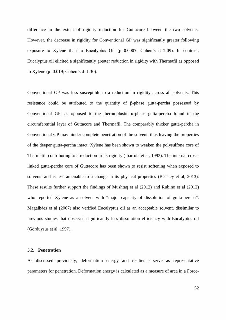
52

difference in the extent of rigidity reduction for Guttacore between the two solvents.

However, the decrease in rigidity for Conventional GP was significantly greater following

exposure to Xylene than to Eucalyptus Oil (p=0.0007; Cohen’s d=2.09). In contrast,

Eucalyptus oil elicited a significantly greater reduction in rigidity with Thermafil as opposed

to Xylene (p=0.019; Cohen’s d=1.30).

Conventional GP was less susceptible to a reduction in rigidity across all solvents. This

resistance could be attributed to the quantity of β-phase gutta-percha possessed by

Conventional GP, as opposed to the thermoplastic α-phase gutta-percha found in the

circumferential layer of Guttacore and Thermafil. The comparably thicker gutta-percha in

Conventional GP may hinder complete penetration of the solvent, thus leaving the properties

of the deeper gutta-percha intact. Xylene has been shown to weaken the polysulfone core of

Thermafil, contributing to a reduction in its rigidity (Ibarrola et al, 1993). The internal cross-

linked gutta-percha core of Guttacore has been shown to resist softening when exposed to

solvents and is less amenable to a change in its physical properties (Beasley et al, 2013).

These results further support the findings of Mushtaq et al (2012) and Rubino et al (2012)

who reported Xylene as a solvent with “major capacity of dissolution of gutta-percha”.

Magalhães et al (2007) also verified Eucalyptus oil as an acceptable solvent, dissimilar to

previous studies that observed significantly less dissolution efficiency with Eucalyptus oil

(Görduysus et al, 1997).

5.2. Penetration

As discussed previously, deformation energy and resilience serve as representative

parameters for penetration. Deformation energy is calculated as a measure of area in a Force-

53

Distance graph whereas resilience is calculated as a measure of area in a Force-Time graph

(see Fig. 3.6).

Any increase in deformation energy following solvent exposure infers that a greater force is

required by the retreatment file when penetrating the GP. The deformation energies of

Conventional GP, Thermafil and Guttacore were significantly reduced with Eucalyptus oil

(p<0.05) and Xylene (p<0.05). The decrease in deformation energy for Conventional GP was

significantly greater for Xylene than for Eucalyptus Oil (p=0.0006; Cohen’s d=2.13). There

was no significant difference between the two solvents for Thermafil and Guttacore. Upon

comparison of the changes in deformation energies, a significantly greater reduction was

observed with Thermafil and Guttacore than with Conventional GP (p<0.05). This is in

accordance with Tanomaru-Filho et al (2010) who demonstrated that Xylene and Eucalyptus

oil presented a more favoured solvent effect on Thermoplastic GP than on Conventional GP.

An increase in resilience denotes that the material will absorb a greater energy of the applied

force before yielding to penetration or fracture. A decrease in file penetration reduces the

surface area of the file that engages the GP. This reduction in contact leads to a decline in the

amount of GP being removed with each successive file withdrawal This increases clinical

procedure time and possibly operator frustration as the retreatment procedure becomes more

arduous to perform.

Eucalyptus oil showed no significant reduction in the resilience of Thermafil and Guttacore,

with an insignificant increase observed with Conventional GP (p=0.37). Following exposure

to Xylene, there was a significant increase in resilience with Conventional GP (p=0.0175),

whilst there was a significant decrease with Guttacore (p=0.0015), and an insignificant

54

reduction with Thermafil (p=0.61). Hence, while the solvents may aid the penetration of

retreatment files into Thermafil and Guttacore, they may actually confound the retreatment

procedure when Conventional GP is present in the canal Nonetheless, with resilience being

closely related to the ability of the polymer chain to rotate freely, additional factors such as

the rate and extent of deformation, the applied force, as well as temperature will also affect

the resilience value of the material (Huson and Maxwell, 2006). However, increasing the

force applied to the retreatment file will amplify the resultant mechanical stresses, which in

turn can lead to instrument separation (Bahcall, 2013).

Conventional GP consists of mainly β-phase gutta-percha and zinc-oxide, whereas Thermafil

and Guttacore have α-phase gutta-percha circumferentially around their respective cores. The

two crystalline phases (α-phase and β-phase) are molecularly both trans isomers, differing

only in single bond configuration and molecular repeat distance. However, the molecular

repeat distance for β-phase gutta-percha is shorter than that of α-phase gutta-percha. This

results in the α-phase being more flexible than the β-phase and contributes to the

vulnerability of α-phase gutta-percha to solvents, as illustrated by Tanomaru-Filho et al in

2010. Both, Thermafil and Guttacore rely on heating to make their circumferential GP

flowable during canal insertion. Heating the material to a temperature range of 46-48oC,

causes the α-phase gutta-percha to transform into β-phase and lose flexibility. Should the

heating temperature exceed 58oC, the gutta-percha then transforms into an irreversible

amorphous phase which then exhibits entirely different mechanical properties (Goodman et

al, 1974; Schilder et al, 1985; Maniglia-Ferreira et al, 2007). Thermal treatment was not used

in the present study and since thermal exposure causes molecular phase transformations, and

changes the bond structure and orientation of the GP, these data may not necessarily reflect

55

the properties of the material at chairside. However, they provide a base reference for

physical changes that occur in GP following solvent exposure.

56

CHAPTER 6

CONCLUSIONS AND RECOMMENDATIONS

The endodontic solvents, Xylene and Eucalyptus oil, have both proven effective in their

ability to significantly change the physical properties of all three types of GP.

Conventional GP is more resistant to changes in its physical properties when compared with

thermoplastic GP forms. Despite the fact that the hardness and deformation energy of

conventional GP does significantly decrease, changes in its resilience may not always prove

beneficial Whilst a decrease in GP hardness may aid its removal from the root canal system,

an increased resilience may in fact hinder penetration and subsequent engagement of the

retreatment file to the GP.

The thermoplastic forms of GP, Thermafil and Guttacore, are vulnerable to endodontic

solvents which alter their physical properties more readily. However, whilst the

circumferential gutta-percha may be amenable to removal, the central core may portray

entirely different properties which will either assist or hinder its removal It is therefore

recommended that this study be repeated using only the core GP of these thermoplastic

materials.

Thermal exposure causes molecular phase transformations, and changes the bond structure

and orientation of the GP. Thus further study is required to assess the changes in the physical

properties that occur following thermal exposure.

57

A greater reduction in the hardness of thermafil GP was observed with Eucalyptus oil, while

no significant difference was found in the interactions between thermafil GP and either

solvent. Conventional GP was susceptible to a significant reduction in hardness with both

solvents, however its penetrability may be compromised by the use of Xylene. No significant

differences were found in the interactions between Guttacore and either solvent. Thus,

considering the toxicity profile of Xylene, and the biocompatibility and antimicrobial effects

of Eucalyptol, Eucalyptus oil is recommended for use during endodontic retreatment.

58

REFERENCES

Azar MR, Khojastehpour LL, Iranpour NN. A Comparison of the Effectiveness of

Chloroform in Dissolving Resilon and Gutta-Percha. J Dent (Tehran). 2011; 8:19-24.

Bahcall J. Remedying and Preventing Endodontic Rotary Nickel-Titanium (NiTi) File

Breakage. Compend Contin Educ Dent. 2013; 34:324-328.

Beasley RT, Williamson AE, Justman BC, Qian F. Time required to remove Guttacore,

Thermafil plus, and thermoplasticized gutta-percha from moderately curved root canals with

Protaper files. J Endod 2013; 39:125-128.

Buchner A, Erdfelder E, Faul F, Lang A. 2009. G*Power (Version 3.1.2)[Computer

program]. http://www.psycho.uniduesseldorf.de/aap/projects/gpower/. Accessed December

2013

Elaissi A, Rouis Z, Salem NA, Mabrouk S, ben Salem Y, Salah KB, Aouni M, Khouja M.

Chemical composition of 8 eucalyptus species' essential oils and the evaluation of their

antibacterial, antifungal and antiviral activities. BMC Complement Altern Med. 2012; 12:81.

Ezzie E, Fleury A, Solomon E, Spears R, He J. Efficacy of retreatment techniques for a resin-

based root canal obturation material J Endod 2006; 32:341-344.

http://www.psycho.uniduesseldorf.de/aap/projects/gpower/

59

Faria-Júnior NB, Loiola LE, Guerreiro-Tanomaru JM, Berbert FL, Tanomaru-Filho M.

Effectiveness of three solvents and two associations of solvents on gutta-percha and resilon.

Braz Dent J. 2011; 22:41-44.

Ferreira JJ, Rhodes JS, Ford TRP. The efficacy of gutta-percha removal using ProFiles. Int

Endod J. 2001; 34:267-274.

Goodman A, Schilder H, Aldrich W. The thermomechanical properties of gutta-percha: II.

The history and molecular chemistry of gutta-percha. Oral Surg Oral Med Oral Pathol. 1974;

37:954-961.

Görduysus MÖ, Tasman F, Tuncer S, Etikan I. Solubilizing efficiency of different gutta-

percha solvents: a comparative study. J Nihon Univ Sch Dent. 1997; 39:133-135.

Gurgel-Filho ED, Feitosa JA, Teixeira FB, de Paula RM, Silva JA, Souza-Filho FJ. Chemical

and X-ray analyses of five brands of dental gutta-percha cone. Int Endod J. 2003; 36:302-

307.

Gutmann JL. The Future of Root Canal Obturation. Dent Today. 2011; 30:128-131.

Gutmann JL, Kuttler S, Niemczyk SP. Root canal obturation: An update. Academy of

General Dentistry. 2010;1-11. http://www.3dfill.com/pdfs/webce090110.pdf. Accessed

March 2014.

Hansen MG. Relative efficiency of solvents used in endodontics. J Endod. 1998; 24:38-40.

http://www.3dfill.com/pdfs/webce090110.pdf

60

Hunter KR, Doblecki W, Pelleu GB. Halothane and eucalyptol as alternatives to chloroform

for softening gutta-percha. J Endod 1991; 17:310-312.

Hülsmann M, Bluhm V. Efficacy, cleaning ability and safety of different rotary NiTi

instruments in root canal retreatment. Int Endod J. 2004; 37:468-476.

Huson MG, Maxwell JM. The measurement of resilience with a scanning probe microscope.

Polym Test 2006; 25:2-11.

Johann JE, Martos J, Silveira LFM, Del Pino FAB. Use of Organic Solvents in Endodontics:

a review. Clinica Pesquisa Odontológica. 2006; 2:393-399.

Ibarrola JL, Knowles KI, Ludlow MO. Retrievability of Thermafil plastic cores using organic

solvents. J Endod 1993; 19:417-418.

Juergens UR, Stober M, Schmidt-Schilling L, Kleuver T, Vetter H: Anti-inflammatory effects

of eucalyptol (1,8-cineole) in bronchial asthma: inhibition of arachidonic acid metabolism in

human blood monocytes ex vivo. Eur J Med Res 1998; 3:407-412.

Kandyala R, Raghavendra SP, Rajasekharan ST. Xylene: An overview of its health hazards

and preventive measures. J Oral Maxillofac Pathol. 2010; 14:1-5.

Kaplowitz GJ. Evaluation of gutta-percha solvents. J Endod. 1990; 16:539-540.

61

Kaplowitz, GJ. Evaluation of the ability of essential oils to dissolve gutta-percha. J Endod.

1991; 17:448-449.

Karlović Z, Anić I, Miletić I, Jukić S, Bošnjak A, Jurić H. Revision of the Endodontic Filling

with Solvents Eucalyptol, Halothane and Orange Oil. Acta stomatologica Croatica. 2001;

35:215-219.

Klatzky RL, Lederman SJ, Hamilton C, Grindley M, & Swendsen RH. Feeling textures

through a probe: Effects of probe and surface geometry and exploratory factors. Percept

Psychophys. 2003; 65:613-631.

Magalhães BS, Johann JE, Lund RG, Martos J, Del Pino FA. Dissolving efficacy of some

organic solvents on gutta percha. Braz Oral Res. 2007; 21:303-307.

Maniglia-Ferreira C, Silva Jr JBA, Paula RCM, Feitosa JPA, Cortez DGN, Zaia AA, Souza

Filho FJ. Brazilian gutta-percha points. Part I: chemical composition and X-ray diffraction

analysis. Braz Oral Res 2005; 19:193-197.

Maniglia-Ferreira C, Gurgel-Filho ED, Silva Jr JBA, Paula RCMD, Feitosa JPA, Gomes

BPFDA, Souza-Filho FJD. Brazilian gutta-percha points. Part II: thermal properties. Braz

Oral Res 2007; 21:29-34.

Marciano J, Michailesco PM. Dental gutta-percha: chemical composition, X-ray

identification, enthalpic studies, and clinical implications. J Endod 1989; 15:149-153.

http://biblio.irb.hr/prikazi-rad?&lang=EN%20Croatian%20Scientific%20Biblography%20CROSBI&rad=103258

http://biblio.irb.hr/prikazi-rad?&lang=EN%20Croatian%20Scientific%20Biblography%20CROSBI&rad=103258

62

Martos J, Gastal MT, Sommer L, Lund RG, Del Pino FA, Osinaga PW. Dissolving efficacy

of organic solvents on root canal sealers. Clin Oral Investig. 2006; 10:50-54.

Metzger Z, Basrani B, Goodis HE. Instruments, materials and devices. In: Cohen S,

Hargreaves K: Pathways of the pulp. 10th Edition. St. Louis, Mosby, 2011. pp.260-261.

Meyer KM, Kollmar F, Schirrmeister JF, Schneider F, Hellwig E. Analysis of shrinkage of

different gutta-percha types using optical measurement methods. Schweiz Monatsschr

Zahnmed. 2006; 116:356-361.

Mitchell P.W. "SEPARATION OF 1, 8-CINEOLE." European Patent No. EP 0125539.

European Patent Office, 1989.

Mushtaq M, Farooq R, Ibrahim M, Khan FY. Dissolving efficacy of different organic

solvents on gutta-percha and resilon root canal obturating materials at different immersion

time intervals. J Conserv Dent. 2012; 15:141-145.

Oyama KON, Siqueira EL, Santos M. Action of Different Solvents on the Gutta-Percha

Cones. ECLER Endod 1999; 1:1-8.

Oyama KO, Siqueira EL, Santos M. In vitro study of effect of solvent on root canal

retreatment. Braz Dent J 2002; 13:208-211.

Prakash R, Gopikrishna V, Kandaswamy D. Gutta-Percha: An Untold Story. Endodontology.

2005; 17:32-36.

63

Rubino GA, Akisue E, Nunes BG, & Gavini G. Solvency capacity of gutta-percha and

Resilon using chloroform, eucalyptol, orange oil or xylene; Capacidade de solvência da guta-

percha e do Resilon utilizando clorofórmio, eucaliptol, óleo de laranja ou xilol. J Health Sci

Inst. 2012; 30:22-25.

Roberts JD and Caserio MC: Basic Principles of Organic Chemistry, 2nd ed. WA Benjamin,

Menlo Park, 1979. Web link: http://www.organicchemistry.com/polymerization-reactions-of-

conjugated-dienes/. Accessed December 2013

SAS Institute Inc., SAS Software, version 9.3 for Windows, Cary, NC, USA: SAS Institute

Inc. (2002-2010).

Schäfer E, Zandbiglari T. A comparison of effectiveness of chloroform and eucalyptus oil in

dissolving root canal sealers. Oral Surg Oral Med Oral Pathol. 2002; 93:611-616.

Schilder H. Filling root canals in three dimensions. Dent Clin North Am 1967; 11:723-744.

Schilder H, Goodman A, Aldrich W. The thermomechanical properties of gutta-percha. 3.

Determination of phase transition temperatures for gutta-percha. Oral Surg Oral Med Oral

Pathol 1974; 38:109-114.

Schilder H, Goodman A, Aldrich W. The thermomechanical properties of gutta-percha. V.

Volume changes in bulk gutta-percha as a function of temperature and its relationship to

molecular phase transformation. Oral Surg Oral Med Oral Pathol 1985; 59:285-296.

http://www.organicchemistry.com/polymerization-reactions-of-conjugated-dienes/

http://www.organicchemistry.com/polymerization-reactions-of-conjugated-dienes/

64

Soares MC, Damiani CE, Moreira CM, Stefanon I, & Vassallo DV. Eucalyptol, an essential

oil, reduces contractile activity in rat cardiac muscle. Braz J Med Biol Res 2005; 38:453-461.

Takarada K, Kimizuka R, Takahashi N, Honma K, Okuda K, Kato T: A comparison of the

antibacterial efficacies of essential oils against oral pathogens. Oral Microbiol Immunol

2004; 19:61-64.

Tamse A, Unger U, Metzger Z, & Rosenberg M. Gutta-percha solvents - a comparative

study. J Endod 1986; 12:337-339.

Tanomaru-Filho M, Orlando Td, Bortoluzzi EA, Silva GF, Tanomaru JM. Solvent capacity of

different substances on gutta-percha and Resilon. Braz Dent J. 2010; 21:46-49.

Tasdemir T, Yildirim T, Celik D. Comparative study of removal of current endodontic

fillings. J Endod. 2008; 34:326-329.

Tsukada G, Tanaka T, Torii M, Inoue K. Shear modulus and thermal properties of gutta

percha for root canal filling. J Oral Rehabil 2004; 31:1139-1144.

Uchida Y, Nakatsuka H, Ukai H, Watanabe T, Liu YT, Huang MY. Symptoms and signs in

workers exposed predominantly to xylene. Int Arch Occup Environ Health 1993; 64:597-605.

Uemura M, Hata G, Toda T, Weine FS. Effectiveness of eucalyptol and d-limolene as gutta-

percha solvents. J Endod 1997; 23:739-741.

65

U.S Department of Health and Human Services. Toxicological profile for xylene, Public

health service, Agency for Toxic Substance and Disease Registry, Clement International

Corporation, 1993.

U.S. Department of Health and Human Services, Public Health Service. Fourth Annual

Report on Carcinogens, PB 85-134663. U.S Government Printing Office, Washington, DC,

1985

Whitworth JM, Boursin EM. Dissolution of root canal sealer cements in volatile solvents. Int

Endod J. 2000; 33:19-24.

Wilcox LR. Endodontic retreatment with halothane versus chloroform solvent. J Endod 1995;

21:305-307.

Wilcox LR, Krell KV, Madison S, Rittman B. Endodontic retreatment: Evaluation of gutta-

percha and sealer removal and canal reinstrumentation. J Endod 1987; 13:453-457.

Wourms JD, Campbell AD, Hicks ML, Pelleu GB. Alternative solvents to chloroform for

gutta percha removal J Endod. 1990; 16:224-226.

66

APPENDIX A

COMPARISON OF THE PHYSICAL PROPERTIES OF THE THREE GP TYPES

FOLLOWING SOLVENT EXPOSURE

The effects of the treatments on the AFTER variables for each of the three dependent

variables was assessed using a general liner model with main effects for solvent and GP type,

a two-factor interaction between solvent and GP type, and experiment day as the blocking

variable. As mentioned previously, the use of room and solvent temperatures as covariates

was also considered, however these remained constant throughout the study. Post-hoc tests

were conducted using the Tukey-Kramer test.

A.1 Rigidity AFTER:

A box-and-whisker plot of the raw data, by GP type and solvent, is shown in Fig A.1.

Fig. A.1 Box-and-whisker plot of the raw data for rigidity following solvent exposure.


Table A.1.

67

Table A.1: Source table for rigidity following solvent exposure.


GP_type 2 2047.30 1023.65 12.99 <.0001

Solvent 2 21069.02 10534.51 133.63 <.0001

GP_type*Solvent 4 5687.94 1421.98 18.04 <.0001

Date 2 7.03 3.51 0.04 0.96

Since the two-factor interaction is significant, we interpret this (and not the main effects).

The Least-Squares means plot is shown in Fig. A.2.

Fig. A.2 Least-Squares means plot for rigidity following solvent exposure.

0

10

20

30

40

50

60

70

80

90

100


Rig

idit

y_A

FTER

: LS

-Me

an

Solvent

Conventional

Guttacore

Thermafil

68

Table A.2 Post hoc tests for Rigidity_AFTER indicating the significant differences in red.



Dependent Variable: Rigidity_AFTER


C / DW

0.640 0.000 <.0001 0.001 <.0001 <.0001 0.001 1.000

C / EO 0.640

0.053 <.0001 0.127 0.001 <.0001 0.124 0.909

C / Xyl 0.0002 0.053

<.0001 1.000 0.887 <.0001 1.000 0.001

G / DW <.0001 <.0001 <.0001

<.0001 <.0001 0.998 <.0001 <.0001

G / EO 0.001 0.127 1.000 <.0001

0.719 <.0001 1.000 0.003

G / Xyl <.0001 0.001 0.887 <.0001 0.719

<.0001 0.697 <.0001

T / DW <.0001 <.0001 <.0001 0.998 <.0001 <.0001

<.0001 <.0001

T / EO 0.001 0.124 1.000 <.0001 1.000 0.697 <.0001

0.002

T / Xyl 1.000 0.909 0.001 <.0001 0.003 <.0001 <.0001 0.002


The lowest rigidity after solvent treatment was obtained with G/X, whose mean

Rigidity_AFTER was not significantly different from C/X, G/EO, or T/EO.

Focusing on the DIFF per material type, we can conclude the following:

C/DW > C/X (Cohen’s d=2.8)

G/DW > G/X, G/EO (Cohen’s d=3.2 and 3.1 respectively)

T/DW > T/X, T/EO (Cohen’s d = 2.7 and 3.9 respectively).

All the effect sizes are classified as ‘large’.

Thus the best combinations of low Rigidity_AFTER solvent treatment, combined with high

change in rigidity as a result of solvent treatment, were G/X, G/EO, and T/EO.

A.2 Deformation Energy AFTER

A box-and-whisker plot of the raw data, by GP type and solvent, is shown in Fig. A.3.

69

Fig. A.3 Box-and-whisker plot of the raw data for deformation energy following solvent

exposure.


Table A.3 below:

Table A.3 Source table for deformation energy following solvent exposure.


GP_type 2 3.01 1.50 3.41 0.039

Solvent 2 108.01 54.01 122.44 <.0001

GP_type*Solvent 4 18.60 4.65 10.54 <.0001

Date 2 0.32 0.16 0.37 0.69

The main effects of GP type and Solvent, as well as their interaction, were significant. We

note that the blocking effect of date was not significant.



70

Fig. A.4 Least-Squares means plot for deformation energy following solvent exposure.

Table A.4 Post hoc tests for Deformation Energy_AFTER indicating the significant

differences in red.



Dependent Variable: Deformation Energy_AFTER


C / DW

0.766 <.0001 0.013 <.0001 <.0001 0.000 0.000 0.011

C / EO 0.766

0.003 <.0001 0.008 <.0001 <.0001 0.038 0.375

C / Xyl <.0001 0.003

<.0001 1.000 0.968 <.0001 0.996 0.710

G / DW 0.013 <.0001 <.0001

<.0001 <.0001 0.993 <.0001 <.0001

G / EO <.0001 0.008 1.000 <.0001

0.900 <.0001 1.000 0.852

G / Xyl <.0001 <.0001 0.968 <.0001 0.900

<.0001 0.576 0.149

T / DW 0.0004 <.0001 <.0001 0.993 <.0001 <.0001

<.0001 <.0001

T / EO 0.0002 0.038 0.996 <.0001 1.000 0.576 <.0001

0.989

T / Xyl 0.011 0.375 0.710 <.0001 0.852 0.149 <.0001 0.989


Possible interpretations:

The lowest deformation energy after solvent treatment was obtained with G/X, whose mean

Deformation Energy _AFTER was not significantly different from C/X, G/EO, T/X or T/EO.

0

1

2

3

4

5

6

7


De

form

atio

n E

ne

rgy_

AFT

ER:

LS-M

ean

Solvent

Conventional

Guttacore

Thermafil

71

Thus the best combinations of low Deformation Energy_AFTER solvent treatment, combined

with high change in deformation energy as a result of solvent treatment, were G/X, C/X,

G/EO, T/X and T/EO.

A.3 Resilience AFTER

A box-and-whisker plot of the raw data, by GP type and solvent, is shown in Fig. A.5.

Fig. A.5 Box-and-whisker plot of the raw data for resilience following solvent exposure.

The overall model was significant: F(10,70)=2.91; p=0.0042. The source table is shown in

Table A.5.

Table A.5 Source table for resilience DIFF following solvent exposure.


GP_type 2 279.75 139.88 4.42 0.016

Solvent 2 129.63 64.81 2.05 0.14

GP_type*Solvent 4 469.43 117.36 3.71 0.009

Date 2 53.81 26.90 0.85 0.43

72

The main effect of GP type, as well as the ‘GP type x Solvent’ interaction, were significant.

We note that the blocking effect of date was not significant.



Fig. A.6 Least-Squares means plot for resilience following solvent exposure.

70

75

80

85

90

95

100

105


Re

silie

nce

_AFT

ER:

LS-M

ean

Solvent

Conventional

Guttacore

Thermafil

73

Table A.6 Post hoc tests for Resilience_AFTER indicating the significant differences in red.



Dependent Variable: Resilience_AFTER


C / DW

0.988 0.996 1.000 0.989 0.003 1.000 0.913 0.998

C / EO 0.988

0.688 0.999 1.000 0.059 1.000 1.000 1.000

C / Xyl 0.996 0.688

0.977 0.724 0.000 0.929 0.432 0.819

G / DW 1.000 0.999 0.977

0.999 0.015 1.000 0.972 1.000

G / EO 0.989 1.000 0.724 0.999

0.070 1.000 1.000 1.000

G / Xyl 0.003 0.059 0.0003 0.015 0.070

0.019 0.169 0.064

T / DW 1.000 1.000 0.929 1.000 1.000 0.019

0.992 1.000

T / EO 0.913 1.000 0.432 0.972 1.000 0.169 0.992

1.000

T / Xyl 0.998 1.000 0.819 1.000 1.000 0.064 1.000 1.000


Possible interpretations:

The lowest resilience after solvent treatment was obtained with G/X, whose mean

Resilience_AFTER was not significantly different from C/EO, G/EO, T/X or T/EO.

Thus the best combinations of low Resilience_AFTER solvent treatment, combined with high

change in resilience as a result of solvent treatment, were G/X, G/EO, and T/EO.

Finally, combining the conclusions from the three physical properties, the best combinations

of low properties AFTER solvent treatment, combined with high change in properties as a

result of solvent treatment, were G/X, G/EO, and T/EO.

74

APPENDIX B

ETHICS WAIVER CERTIFICATE

75

APPENDIX C

FACULTY PROTOCOL APPROVAL

HARDNESS AND PENETRATION OF GUTTA PERCHA WHEN …

Documents

Transcript of HARDNESS AND PENETRATION OF GUTTA PERCHA WHEN …