TEC-SR-7

Handbook forTransformation ofDatums, Projections,Grids and CommonCoordinate Systems

January 1996

Approved for public release; distribution is unlimited.

U.S. Army Corps of EngineersTopographic Engineering Center7701 Telegraph RoadAlexandria. VA 22315-3864

Destroy this report when no longer needed.Do not return it to the originator.

The findings in this report are not to be construed as an official Department of the Armyposition unless so designated by other authorized documents.

The citation in this report of trade names of commercially available products does notconstitute official endorsement or approval of the use of such products.

Form ApprovedREPORT DOCUMENTATION PAGE OMBNo.0704-0188

Public reporting burden for this collection of information is estimated to average 1 hour per response, including the time for reviewing instructions, searching existing data sources,

gathering and maintaining the data needed, and completing and reviewing the collection of information. Send comments regarding this burden estimate or any other aspect of thiscollection of information, including suggestions for reducing this burden, to Washington Headquarters Services, Directorate for Information Operations and Reports, 1215 JeffersonDavis Highway, Suite 1204, Arlington, VA 22202-4302, and to the Office of Management and Budget, Paperwork Reduction Project (0704-0188), Washington, DC 20503.

1. AGENCY USE ONLY (Leave blank) 2. REPORT DATE 3. REPORT TYPE AND DATES COVERED

January 1996 Handbook May 1991 - July 1995

4. TITLE AND SUBTITLE 5. FUNDING NUMBERSHandbook for Transformation of Datums, Projections, Grids QE5113UD01and Common Coordinate Systems

6. AUTHOR(S)See Preface

7. PERFORMING ORGANIZATION NAME(S) AND ADDRESS(ES) 8. PERFORMING ORGANIZATIONU.S. Army Topographic Engineer Center REPORT NUMBER

7701 Telegraph Road TEC-SR-7Alexandria, VA 22315-3864

9. SPONSORING / MONITORING AGENCY NAME(S) AND ADDRESS(ES) 19. SPONSORING / MONITORINGAGENCY REPORT NUMBER

11. SUPPLEMENTARY NOTES

Beneficial comments or information that may be of use in improving this documentshould be addressed to the Standards Division of the Digital Concepts & AnalysisCenter at the above address.

12a. DISTRIBUTION / AVAILABILITY STATEMENT 12b. DISTRIBUTION CODE

Approved for public release; distribution is unlimited. UNLIMITED

13. ABSTRACT (Maximum 200 words)This document provides Army orginizations and agencies with general guidance onselecting the appropriate methods for shifting between local geodetic datums and theWorld Geodetic System (WGS), and for converting Cartesian and map projectioncoordinates to and from geodetic coordinates. This guidance is provided to aid theArmy community in selecting datum shift algorithms, in developing, selecting, andmaintaining software using these algorithms, and in implementing this software tosupport operational units. Equations are furnished for map projections and datumscommonly used within the Army, and references are provided for other, less commonlyencountered, map projections and datums.

14. SUBJECT TERMS 15. NUMBER OF PAGESCartography Datums Projections 170Geodesy Coordinates 16. PRICE CODE

17. SECURITY CLASSIFICATION 18. SECURITY CLASSIFICATION 19. SECURITY CLASSIFICATION 20. LIMITATION OF ABSTRACTOFREPORT OF THIS PAGE OFABSTRACT

Unclassified Unclassified Unclassified

NSN 7540-01-280-5500 Standard Form 298 (Rev. 2-89)Prescribed by ANSI Std. Z39-18298-102

TABLE OF CONTENTS

PAGE

LIST OF FIGURES ixLIST OF TABLES xiEXECUTIVE SUMMARY xiiiPREFACE xv

1. SCOPE 11.1 Scope 11.2 Applicability 11.3 Application guidance 1

2. REFERENCED DOCUMENTS 22.1 Government documents 22.1.1 Specifications, standards and handbooks 22.1.2 Other government documents, drawings and 2

publications2.2 Non-government publications 42.3 Order of precedence 4

3. DEFINITIONS AND UNITS 53.1 Acronyms 53.2 Terms 53.2.1 Convergence of the meridian (C) 53.2.2 Coordinate 53.2.3 Datum 53.2.3.1 Horizontal datum 63.2.3.2 Vertical datum 63.2.4 Earth-fixed 63.2.5 Elevation (orthometric height, H) .63.2.6 Ellipsoid 63.2.7 Equator 63.2.8 Equipotential surface 63.2.9 Geocentric Cartesian coordinates 63.2.10 Geodetic coordinates (geodetic position) 63.2.11 Geodetic height (ellipsoidal height, h) 63.2.12 Geodetic latitude (*) 73.2.13 Geodetic longitude (k) 73.2.14 Geographic coordinates 73.2.15 Geoid 73.2.16 Geoid separation (N) 73.2.17 Grid reference system 73.2.18 Map projection 73.2.19 Map scale 73.2.20 Meridian 73.2.21 Military Grid Reference System (MGRS) 73.2.22 Orthometric height 83.2.23 Parallel 83.2.24 Prime (initial) meridian 83.2.25 Reference ellipsoid 83.2.26 Scale factor (projection) 83.3 Units 8

iii

TABLE OF CONTENTS

PAGE3.4 Sign conventions 83.5 Unit conversion factors 83.5.1 Degrees and radians 93.5.2 Specifying the unit of angular measure 9

4. FUNDAMENTAL CONCEPTS 104.1 Introduction 104.2 Reference surfaces 114.2.1 Reference ellipsoid 114.2.2 Geoid 114.2.3 Relationships among topography, the geoid, 11

and the reference ellipsoid4.3 Earth-fixed coordinate systems 134.3.1 Cartesian coordinates (X, Y, Z) 134.3.2 Cartesian coordinate system/reference ellipsoid

relationship 134.3.2.1 First eccentricity and flattening 154.3.2.2 Ellipsoid parameters 154.3.3 Geodetic coordinates (0, X, h) 154.3.3.1 Latitude and longitude limits 154.3.4 Coordinate conversion 154.3.4.1 Geodetic to Cartesian coordinate conversion 164.3.4.2 Cartesian to geodetic coordinate conversion 164.3.4.2.1 Finding X 164.3.4.2.2 Finding 4 164.3.4.2.3 Calculating h 174.4 Representation of Geodetic Coordinates 184.5 Height Relationships 184.5.1 Elevations 184.5.2 Geoid separation 184.5.3 The relationships among H, h, and N 184.5.3.1 Notational use of H and h 18

5. GEODETIC SYSTEMS AND DATUMS 195.1 Introduction 195.2 Geodetic (horizontal) datums 195.2.1 Background 195.2.2 Geodetic datums and WGS 84 195.3 Vertical datums and elevations 205.3.1 Background 205.3.2 Vertical datums and mean sea level (MSL) 205.3.3 Relationship between local, vertical and horizontal

datums 205.4 World Geodetic System 1984 (WGS 84) 205.5 WGS 84 referenced elevations 21

6. DATUM SHIFTS 226.1 Introduction 226.1.1 Shifting between two local datums 226.1.1.1 Shifting from NAD 27 to NAD 83 226.2 Seven-parameter geometric transformation 236.2.1 Transformation to WGS 84 Cartesian coordinates 23

iv

TABLE OF CONTENTS

PAGE6.2.2 Transformation to LGS Cartesian coordinates 246.2.3 Parameter Values 246.2.4 Accuracy of seven-parameter transformation 24

6.3 Three-parameter (AX, AY, AZ) geometric 24transformation

6.3.1 Transformation to WGS 84 Cartesian coordinates 256.3.1.1 Three-step method: Transformation to 25

WGS 84 geodetic coordinates6.3.2 Transformation to local geodetic coordinates 266.3.2.1 Three-step method: Transformation to 26

local geodetic coordinates6.3.3 Molodensky shifts 266.3.4 AX, AY, AZ shift values 28

6.3.5 Accuracy of AX, AY, AZ shift parameters 286.3.6 Local datum distortion 296.4 WGS 72 to WGS 84 transformation 296.4.1 Selecting a conversion method 306.4.2 Direct WGS 72 to WGS 84 transformation 306.4.2.1 Conversion equations 306.4.2.2 Estimated errors ( 0 Aý, 'AXAh) 32

6.4.3 Two-step WGS 72 to WGS 84 transformation 326.5 Approximating geodetic heights for datum

transformation 326.6 Multiple Regression Equations 336.7 Vertical datum shifts 336.7.1 Satellite-derived WGS 72 elevations based 33

on measured WGS 72 geodetic heights6.7.2 Survey-derived elevations 336.8 Unlisted datums 33

7. MAP PROJECTIONS 347.1 Introduction 347.1.1 The map projection process 347.1.2 Properties of projections 347.1.3 Mapping equations 347.1.4 Conformal projection 347.1.5 Scale factor 347.1.6 Map scale 357.1.7 Convergence of the meridian 357.1.8 Information sources 357.2 Mercator projection 357.2.1 Meridians and parallels 357.2.2 Mercator mapping equations 367.2.2.1 Finding (x,y) 367.2.2.2 Point scale factor and convergence 37

of the meridian7.2.2.3 Finding (O,X) 377.2.3 Accuracy 387.2.4 Area of coverage 387.3 Transverse Mercator (TM) projection 38

v

TABLE OF CONTENTS

PAGE7.3.1 Meridians and parallels 387.3.2 Transverse Mercator mapping equations 397.3.2.1 Finding (x,y) 397.3.2.2 Finding (0,x) 407.3.2.2.1 Finding the footpoint latitude (01) 40

7.3.2.2.2 Finding (0,%) from 01 417.3.2.3 Point scale factor as a function of 42

x and 017.3.2.4 Point scale factor as a function of 42

(0 X)7.3.2.5 Convergence of the meridian in terms of 42

x and 017.3.2.6 Convergence of the meridian in terms of 42

"(0, 20d7.3.3 Accuracy 437.3.4 Area of coverage 437.4 Universal Transverse Mercator (UTM) projection 437.4.1 UTM zones 437.4.1.1 Finding the UTM zone and central meridian 447.4.1.2 Non-standard width UTM zones 457.4.2 Reference source 457.4.3 UTM equations 457.4.3.1 Finding UTM coordinates (Xu•, YUTM) 457.4.3.2 Computing geodetic coordinates 457.4.3.3 Discontinuity 467.4.4 Accuracy 467.4.5 Area of coverage 467.5 Lambert Conformal Conic projection 467.5.1 Lambert Conformal Conic with two standard parallels 477.5.1.1 Finding (x,y) 477.5.1.2 Finding (O,X) with two standard parallels 487.5.2 Lambert Conformal Conic with one standard parallel 497.5.2.1 Finding (x,y) 497.5.2.2 Finding (O,X) with one standard parallel 507.5.3 Scale factor and convergence 507.5.4 Accuracy 507.5.5 Area of coverage 507.6 Polar Stereographic projection 517.6.1 Polar Stereographic mapping equations 517.6.1.1 Finding (x,y) 517.6.1.2 Finding (0,x) 517.6.1.3 Alternate method for finding 4 537.6.1.4 Finding the point scale factor 547.6.1.5 Finding the convergence of the meridian 547.6.2 Accuracy 547.6.3 Area of coverage 547.7 Universal Polar Stereographic (UPS) projection 547.7.1 Universal Polar Stereographic (UPS) mapping equations 557.7.2 Finding (0,x) 55

vi

TABLE OF CONTENTS

PAGE7.7.3 Finding point scale factor and convergence 57

of the meridian7.7.4 Accuracy 577.7.5 Area of coverage 577.8 The U.S. Military Grid Reference System (MGRS) 577.8.1 MGRS coordinates in the UTM area 577.8.2 MGRS coordinates in the UPS area 587.9 The World Geographic Reference System (GEOREF) 637.10 Non-standard grids 637.11 Modification to map projections 63

8. SELECTIONS OF TECHNIQUES, SOFTWARE DEVELOPMENT, 66AND TESTING

8.1 The general conversion process 668.1.1 Application of the general conversion process 708.1.2 Procedural examples 708.1.2.1 Example 8.1 Horizontal geodetic coordinate-based

datum shifts 70

8.1.2.2 Example 8.2 WGS 84 Cartesian coordinate to locallatitude, longitude, and elevation 71

8.1.2.3 Example 8.3 Local latitude, longitude, and elevationto WGS 84 latitude, longitude, andelevation 72

8.2 Choosing a datum shift method 738.2.1 Parameter availability 748.2.2 Accuracy 748.2.3 Implementation issues 758.2.3.1 Preferred shift methods 768.2.3.2 Software testing 768.3 Error Analysis 778.3.1 System model 778.3.2 Error estimates 788.3.2.1 Error types 798.3.3 Reformulation 798.3.4 Error propagation 808.3.5 Example 818.4 Numerical examples 858.4.1 Example 8.4 Convert WGS 84 geodetic coordinates

to Universal Transverse Mercatorcoordinates in the NAD 27 referencesystem using a three-step datum shift 85

8.4.2 Example 8.5 Convert WGS 84 geodetic coordinatesto geodetic coordinates in the NAD 27reference system using the standardMolodensky method 88

8.4.3 Example 8.6 Convert WGS 84 geodetic coordinatesto Mercator projection coordinates 90

8.4.4 Example 8.7 Convert Mercator projection

vii

TABLE OF CONTENTS

PAGEcoordinates in the WGS 84 referencesystem to WGS 84 geodetic latitudeand longitude 90

8.4.5 Example 8.8 Convert Universal TransverseMercator coordinates in the NAD 27reference system to NAD 27 geodeticlatitude and longitude 92

8.4.6 Example 8.9 Convert WGS 84 latitude andlongitude to Lambert Conformal coordinatesusing two standard parallels 94

8.4.7 Example 8.10 Convert Lambert Conformal projection(with two standard parallels) coordinatesin the WGS 84 reference system to WGS 84geodetic latitude and longitude 96

8.4.8 Example 8.11 Convert geodetic latitude andlongitude on the International Ellipsoidto Universal Polar Stereographiccoordinates 98

8.4.9 Example 8.12 Convert Universal Polar Stereographiccoordinates to geodetic latitude andlongitude 99

8.5 List of test points 101

9. NOTES 1039.1 Intended use 1039.2 Subject term (key word) listing 103

APPENDICES PAGE

A. Reference Ellipsoid Parameters 105B. AX, AY, AZ Datum Shift Parameters 107C. Datum List 129D. WGS 84 Geoid Separation Computation 145E. Seven-parameter Geometric Datum Shifts 149F. Old Hawaiian Datum with International Ellipsoid 151

viii

LIST OF FIGURES

PAGE

4.1 The relationship between the reference 12ellipsoid, the geoid, and the physicalsurface of the earth.

4.2 The geometric relationship between 14Cartesian and geodetic coordinates.

6.1 Relationship between coordinate axis in a 23seven-parameter geometric transformation.

6.2 Relationship between coordinate axis in a 25three-parameter geometric transformation.

7.1 Meridians and parallels in the Mercator projection. 36

7.2 Meridians and parallels in the Transverse MercatorProjection. X0 is the central meridian. 39

7.3 Meridians and parallels (dashed) and 44a Universal Transverse Mercator Grid.

7.4 Meridians and parallels in the Lambert 47Conformal Conic Projection.

7.5 Meridians and parallels in the Universal 51Polar Stereographic Projection.

7.6 Meridians and parallels imposed on a 55

Universal Polar Stereographic grid.

7.7 UTM area grid for MGRS 59

7.8 UTM area grid for MGRS 60

7.9 North UPS area grid for MGRS 61

7.10 South UPS area grid for MGRS 62

8.1 A map projection to geodetic datum 66conversion. Height information for Hand h is not included in the conversion.

8.2 Coordinate conversions within a datum. 67

8.3 Datum shifts. 68

8.4 The general conversion process. 69

8.5 System Model 84

ix

LIST OF FIGURES

PAGE

D.1 Coordinate System Associated with Geoid Separation Bi-Linear Interpolation Method 146

x

LIST OF TABLES

Page

3.1 Conversion Factors 9

6.1 Selection of WGS 72 to WGS 84 Transformation Method 30

7.1 Non-Standard Zone Limits 45

8.1 Accuracy Guidance for Equations 79

8.2 Probability Level Conversion Factors 81

A.1 Reference Ellipsoids 106

B.1 Ellipsoid Center Shift Transformation 108Parameters

C.1 Countries and their Associated Datums 130

D.1 WGS 84 Geoid Separations 147

E.1 Seven Parameter Local Geodetic System to WGS 84 150Datum Transformation

xi

EXECUTIVE SUMMARY

This document provides Army organizations and agencies with general guidance on selecting theappropriate methods for shifting between local geodetic datums and the World Geodetic System(WGS), and for converting Cartesian and map projection coordinates to and from geodeticcoordinates. This guidance is provided to aid the Army community in selecting datum shiftalgorithms, in developing, selecting, and maintaining software using these algorithms, and inimplementing this software to support operational units. Equations are furnished for mapprojections and datums commonly used within the Army, and references are provided for other,less commonly encountered, map projections and datums.

Beneficial comments (corrections, recommendations, additions, deletions) or information thatmay be of use in improving this document should be addressed to the Standards Division of theDigital Concepts & Analysis Center (DCAC) at the Topographic Engineering Center (TEC).

Mail: U.S. Army Topographic Engineering Center, ATTN: CETEC-PD-DS, 7701 Telegraph

Road, Alexandria, VA 22315-3864.

Fax: ATTN: Standards Division, DCAC (703) 355-2991

Phone: (703) 355-2761

NEW PHONE NUMBERS!voice (703)428-6761fax (703)428-6991

xiii

PREFACE

This report was funded under the U.S. Army Topographic Engineering Center's (TEC) DigitalTopographic Data Standards Program.

This report was co-authored at TEC by the following individuals:

Frederick GloecklerRichard JoyJustin SimpsonDaniel Specht

The report is based on a draft of the Military Handbook, Datums, Projections, Grids andCommon Coordinate Systems, Transformation of (MIL-HDBK-600008), and was revised duringthe period July 1994 through July 1995. This Technical Report uses material from MIL-HDBK-600008 co-authored by:

James AckeretFred EschChris GardFrederick GloecklerDaniel OimoenJuan PerezMAJ Harry RossanderJustin SimpsonJoe WattsTom Witte

This work was performed under the previous supervision of Juan Perez, and Richard AHerrmann and the current supervision of John W. Hale, Chief, Standards Division and Regis J.Orsinger, Director, Digital Concepts and Analysis Center.

Mr. Walter E. Boge was Director and COL Richard G. Johnson was Commander and DeputyDirector of TEC at the time of publication of this report.

xv

1. SCOPE

1.1 Scope. This Technical Report provides methods andparameter values to shift positions between approximately 113geodetic datums and provides methods for converting betweengeodetic coordinates, Cartesian coordinates and map projectioncoordinates. Guidance is provided on selecting methodsappropriate to the application, and on developing and testingsoftware to implement these conversions.

1.2 Applicability. The methods provided in this TechnicalReport are used for a wide range of Army mapping, charting, andpositioning applications. Equations are furnished for the mapprojections commonly used within the Army. References areprovided for other map projections that occasionally may beencountered. Special high accuracy applications such asengineering, construction, and real estate boundary surveys areoutside the scope of this Technical Report. Appendix B providesdatum shift parameters for approximately 113 datums that arecurrently available from the Defense Mapping Agency (DMA).However, many more local datums exist. For guidance on datumshift applications or for datum shift parameters not covered bythis Technical Report, contact TEC [address given in the preface].

1.3 ADDlication auidance. Transformation methods andparameters should be appropriate to the application. A systemanalyst should do a thorough evaluation of the system requirementsbefore developing detailed specifications. This evaluation shouldconsider the intended use, data types, formats, and requiredaccuracy of the output mapping, charting, and geodesy (MC&G) data,as well as the source and accuracy of the input data. Also, any .hardware constraints must be considered. The methods presented inthis Technical Report can then be examined for how well they canmeet or be adapted to meet the requirements. Where more than onemethod will satisfy a basic requirement, give priority to Army-preferred methods for standardization purposes. Additionalapplication guidance is furnished in Section 8.

1

2. REFERENCED DOCUMENTS

2.1 Government documents.

2.1.1 Specifications: standards. and handbooks. Thefollowing specifications, standards, and handbooks form a part ofthis document to the extent specified herein.

SPECIFICATIONS. None

STANDARDS.

MIL-STD-2401 Department of Defense World GeodeticSystem(WGS) (1994)

STANAG 2211 Geodetic Datums, ellipsoids, grids and(Fifth Edition) grid references (1991)

HANDBOOKS. None

2.1.2 Other Government documents. drawings. andpubhinAtinns. The following other Government documents, drawings, andpublications form a part of this document to the extent specifiedherein. Unless otherwise specified, the issues are those cited in thesolicitation. The date in parentheses indicates for each document theedition that was used in preparation of this Technical Report.

Document ID/Agency Title

DMA Department of Defense Glossary ofMapping, Charting, and Geodetic Terms,Fourth Edition. (1981)

DMA TM 8358.1 Datums, Ellipsoids, Grids, andGrid Reference Systems, (1990)

DMA TM 8358.2 The Universal Grids: UniversalTransverse Mercator (UTM) andUniversal Polar Stereographic (UPS).(1989)

2

DMA Instruction 8000.1 Geodetic and Geophysical Signwith change 1, 4 Aug 92 Conventions and Fundamental Constants.

(1988)

Geological Survey Map Projections - A Working Manual.Professional Paper 1395 (Snyder, 1987)

NOAA Manual NOS NGS 5 State Plane Coordinate System of 1983.(Stem, 1989)

NSWC/DL TR-3624 Map Projection Equations. (Pearson,1977)

U.S. Department of Conformal Projections in Geodesy andCommerce, Coast and Cartography. (Thomas, 1979)Geodetic Survey,Special PublicationNo. 251

Engineer Technical Engineering and Design Conversion toLetter No. 1110-1-147 North American Datum of 1983 (1990)

Federal Register Notice To Adopt Standard Method forv. 55, no. 155, Friday, Mathematical Horizontal DatumAugust 10, 1990 Transformation (NOAA, 1990)Docket No. 900655-0165

Copies of; DMA Instruction 8000.1 and GS Professional Paper 1395 areavailable from USGS, Branch of Distribution, Box 25286, Denver CO80225. Copies of DoD Glossary of Mapping, Charting, and GeodeticTerms; DMA TM 8358.1; and DMA TM 8358.2 are available from theDirector, DMA Combat Support Center, ATTN: CCOR, 6001 MacArthurBoulevard, Bethesda MD 20816-5001. Copies of the NOAA Manual NOS NGS5 and the Coast and Geodetic Survey Special Publication No. 251 areavailable from National Geodetic Information Branch, N/CG174, NationalGeodetic Survey, 1315 East-West Highway, Silver Spring MD 20910.Copies of NSWC/DL TR 3624 (Accession Document Number = AD A037 381 onpaper, or GIDEP #E151-2353 on cartridge) are available on from DefenseTechnical Information Center, Bldg. 5, Cameron Station, Alexandria, VA22304-6145. Copies of ETL 1110-1-147 are available through theDepartment of the Army, U.S. Army Corps of Engineers, Washington, D.C.203140-1000. Copies of STANAG 2211 and MIL-STD 2401 are availablefrom the Defense Printing Service, ATTN: DODSSP, 700 Robbins Ave, Bld4D Philadelphia PA 19111.

3

2.2 Non-Government publications.

Heiskanen, Weikko A., and Helmut Moritz; Physical Geodesy;Institute of Physical Geodesy, Technical University, Graz,Austria; 1967.

Krakiwsky, Edward J.; Conformal Map Projections in Geodesy;Department of Surveying Engineering, University of New Brunswick,Fredrickton, N.B., Canada; September, 1973.

Rapp, Richard H.; Geometric Geodesy - Part I; Department ofGeodetic Science and Surveying, The Ohio State University,Columbus, Ohio; 1984.

Rapp, Richard H.; Geometric Geodesy - Part II; Department ofGeodetic Science and Surveying, The Ohio State University,Columbus, Ohio; 1987.

2.3 Order of precedence. MIL-STD-2401 shall takeprecedence for all matters concerning WGS 84 and datum shiftparameters. Nothing in this document, however, supersedesapplicable laws and regulations unless a specific exemption hasbeen obtained.

4

3. DEFINITIONS AND UNITS

3.1 Acronyms. The acronyms used in this Technical Reportare defined as follows:

a. BIH Bureau International de l'Heureb. CONUS continental United Statesc. CTP Conventional Terrestrial Poled. DMA Defense Mapping Agencye. DoD Department of Defensef. DTED Digital Terrain Elevation Datag. ECEF earth-centered, earth-fixedh. GPS Global Positioning Systemi. LGS local geodetic systemj. MGRS Military Grid Reference Systemk. MC&G mapping, charting and geodesy1. MRE multiple regression equationm. MSL mean sea leveln. NAD 27 North American Datum 1927o. NAD 83 North American Datum 1983p. NGS National Geodetic Surveyq. NGVD 29 National Geodetic Vertical Datum of 1929r. NOAA National Oceanic and Atmospheric

Administrations. NOS National Ocean Surveyt. NSWC/DL Naval Surface Weapons Center/Dahlgren

Laboratoryu. TM Transverse Mercatorv. UPS Universal Polar Stereographicw. UTM Universal Transverse Mercatorx. WGS 72 World Geodetic System 1972y. WGS 84 World Geodetic System 1984

3.2 Terms.

3.2.1 Converqence of the meridian (Y). The angle betweenthe projection of the meridian at a point on a map and theprojection North axis (typically represented by the y axis of theprojection). The convergence of the meridian is positive in theclockwise direction.

3.2.2 Coordinate. Linear or angular quantities thatdesignate the position that a point occupies in a given referenceframe or system. Also used as a general term to designate theparticular kind of reference frame or system, such as Cartesiancoordinates or spherical coordinates.

3.2.3 Datum. Any numerical or geometrical quantity or setof such quantities specifying the reference coordinate system usedfor geodetic control in the calculation of coordinates of pointson the earth. Datums may be either global or local in extent. Alocal datum defines a coordinate system that is used only over a

5

region of limited extent. A global datum specifies the center ofthe reference ellipsoid to be located at the earth's center ofmass and defines a coordinate system used for the entire earth.

3.2.3.1 Horizontal datum. A horizontal datum specifies thecoordinate system in which latitude and longitude of points arelocated. The latitude and longitude of an initial point, theazimuth of a line from that point, and the semi-major axis andflattening of the ellipsoid that approximates the surface of theearth in the region of interest define a horizontal datum.

3.2.3.2 Vertical datum. A vertical datum is the surface towhich elevations are referred. A local vertical datum is acontinuous surface, usually mean sea level, at which elevationsare assumed to be zero throughout the area of interest.

3.2.4 Earth-fixed. Stationary with respect to the earth.

3.2.5 Elevation. Vertical distance measured along the localplumb line from a vertical datum, usually mean sea level or thegeoid, to a point on the earth. Often used synonymously withorthometric height.

3.2.6 Ellipsoid. The surface generated by an ellipserotating about one of its axes. Also called ellipsoid ofrevolution.

3.2.7 Eauator. The line of zero geodetic latitude; thegreat circle described by the semi-major axis of the referenceellipsoid as it is rotated about the semi-minor axis.

3.2.8 Eauipotential surface. A surface with the samepotential, usually gravitational potential, at every point; alevel surface.

3.2.9 Geocentric Cartesian coordinates. Cartesiancoordinates (X, Y, Z) that define the position of a point withrespect to the center of mass of the earth.

3.2.10 Geodetic coordinates (aeodetic position). Thequantities of latitude, longitude, and geodetic height (0, X ,h)that define the position of a point on the surface of the earthwith respect to the reference ellipsoid. Also, imprecisely,called geographic coordinates (See also geographic coordinates).

3.2.11 Geodetic heiaht (ellipsoidal height, h). The heightabove the reference ellipsoid, measured along the ellipsoidalnormal through the point in question. The geodetic height ispositive if the point is outside the ellipsoid.

6

3.2.12 Geodetic latitude (•). The angle between the planeof the Equator and the normal to the ellipsoid through thecomputation point. Geodetic latitude is positive north of theequator and negative south of the Equator (See figure 4.2).

3.2.13 Geodetic lonaitude (%). The angle between the planeof a meridian and the plane of the prime meridian. A longitudecan be measured from the angle formed between the local and primemeridians at the pole of rotation of the reference ellipsoid, orby the arc along the Equator intercepted by these meridians. Seefigure 4.2.

3.2.14 GeoaraDhic coordinates. The quantities of latitudeand longitude that define the position of a point on the surfaceof the earth. See also geodetic coordinates.

3.2.15 Geoid. The equipotential surface of the earth'sgravity field approximated by undisturbed mean sea level of theoceans. The direction of gravity passing through a given point onthe geoid is perpendicular-to this equipotential surface.

3.2.16 Geoid separation (N). The distance between the geoidand the mathematical reference ellipsoid as measured along theellipsoidal normal. This distance is positive outside, ornegative inside, the reference ellipsoid. Also called geoidalheight; undulation of the geoid. See figure 4.1.

3.2.17 Grid reference system. A plane-rectangularcoordinate system usually based on, and mathematically adjustedto, a map projection in order that geodetic positions (latitudesand longitudes) may be readily transformed into plane coordinatesand the computations relating to them may be made by the ordinarymethods of plane surveying (see also 3.2.21).

3.2.18 MaD Droýection. A function relating coordinates ofpoints on a curved surface (usually an ellipsoid or sphere) tocoordinates of points on a plane. A map projection may beestablished by analytical computation or, less commonly, may beconstructed geometrically.

3.2.19 Mar scale. The ratio between a distance on a map andthe corresponding actual distance on the earth's surface.

3.2.20 Meridian. A north-south reference line, particqlarlya great circle through the geographical poles of the earth, fromwhich longitudes and azimuths are determined; or the intersectionof a plane forming a great circle that contains both geographicpoles of the earth, and the ellipsoid.

3.2.21 Military Grid Reference System (MGRS). MGRS is asystem developed by DMA for usage with UTM and UPS projections.

7

3.2.22 Orthometric height. See elevation.

3.2.23 Parallel. A line on the earth, or a representationthereof, that represents the same latitude at every point.

3.2.24 Prime (initial) meridian. A meridian from which thelongitudes of all other meridians are reckoned. This Meridian, oflongitude 00, was traditionally chosen to pass through theGreenwich Observatory in Greenwich, England. For new refinedcoordinate systems, the location of the prime meridian is definedby the International earth Rotation Service, Paris, France.

3.2.25 Reference ellipsoid. An ellipsoid whose dimensionsclosely approach the dimensions of the geoid; the exact dimensionsare determined by various considerations of the section of theearth's surface concerned. Usually a bi-axial ellipsoid ofrevolution.

3.2.26 Scale factor (Drolection). A multiplier for reducinga distance in a map projection to the actual. distance on thechosen reference ellipsoid.

3.3 Units. In this Technical Report all distances areexpressed in meters. Angles are expressed in degrees, radians orthe combination of degrees, minutes, and seconds.

3.4 Sian conventions. The sign conventions used in thisTechnical Report are defined as follows:

a. Elevation. Positive outside or above the vertical datum,negative inside or below the datum.

b. Geodetic heiaht. Positive outside the referenceellipsoid, negative inside the reference ellipsoid.

c. Geodetic latitude. Positive in the northern hemisphere,negative in the southern hemisphere.

d. Geodetic longitude. Zero at the prime meridian, positive00 to 1800, eastward from the prime meridian, and negative00 to 1800, westward from the prime meridian.

e. Geoid seoaration. Positive outside the reference

ellipsoid, negative inside the reference ellipsoid.

f. Cartesian Z. Positive in the northern hemisphere.

3.5 Unit conversion factors. The standard unit of distancemeasurement is the meter. However, MC&G products in many parts ofthe world were produced using other units of measurement. Theuser must ascertain the units used in non-standard products andappropriately scale them for use in the equations given in this

8

technical report. Some commonly used conversion factors are

listed in Table 3.1.

TABLE 3.1 Conversion Factors.

1 meter = 3.28083333333 U.S. Survey feet= 3.28083989501 International feet

1 International foot = 0.3048 meter (Exact)1 U.S. Survey foot = 1200/3937 meter (Exact)

= 0.30480060960 meter1 Int'l Nautical mile = 1852 meters (Exact)

= 6076.10333333 U.S. Survey feet= 6076.11548556 International feet

1 Int'l Statute mile = 1609.344 meters (Exact)= 5280 International feet (Exact)

1 degree = 60 minutes1 degree = 3600 seconds1 minute = 60 seconds6400 U.S. mils = 360 degrees

3.5.1 Dearees and radians. A circle contains 360 degrees oi2n radians. If an angle contains d degrees or, equivalently, rradians, then d and r are related by

r = 18d (3.1)

3.5.2 Specifyina the unit of anaular measure. In thisTechnical Report the unit of angular measure will be specified ifit matters. A general rule of thumb is that angles must be inradians in an equation that was derived using calculus andtrigonometry. Radians are the usual units in computer evaluationof trigonometric functions.

9

4. FUNDAMENTAL CONCEPTS

4.1 Introduction. An understanding of geodesy helps oneunderstand how to represent the locations of points on or aboutthe surface of the earth. Terms printed in boldface are definedin Section 3.2.

a. The location of a point is described by a set ofcoordinates. Some types of coordinates, such asCartesian (see Section 4.3.1), uniquely identifythree-dimensional locations of points in space. Theiruse is computationally efficient in many applications.However, users often have difficulty visualizing therelationship of Cartesian coordinates to the surface ofthe earth. Geodetic coordinates (see Section4.3.3) make visualization easier by providinghorizontal coordinates on the surface of a figureapproximating the shape of the earth and a vertical(height) coordinate above or below the referencesurface.

b. Geodetic coordinates are defined by a geodeticreference system. A geodetic reference systemincludes, but is not limited to, a reference surface(usually an ellipsoid) and a set of parameterspositioning and orienting the reference surface withrespect to the earth. Over the years, many geodeticreference systems have been developed for variouslocalities. These systems are often called local datumsand are not rigorously tied to each other.

c. When applications require that two or more points belocated in a common reference system, transformationbetween two coordinate systems may be needed. Forexample: both weapon and target must be located in thesame reference system if the indirect fire computationsare to be valid. As the ranges of weapons and targetacquisition systems increased and positional data werederived from multiple sources, commanders often wereconfronted with the problem of using positions on morethan one reference system. With the advent ofsatellite geodesy one can establish global geodeticreference systems and take measurements thatallow local datums to be related to the globalsystem. The standard global reference system forDoD is the World Geodetic System 1984 (WGS 84). Theprocess of relating one reference system to another iscalled a datum shift, or datum transformation.

10

d. Coordinates generally are represented alpha-numerically (e.g. latitude 380 51' 22.45"N andlongitude 770 26' 34.56"W). Position data for an areaoften are represented graphically, as on a map. Theplanar representation on a map provides a distortedview of features on the curved earth's surface.Geodesists have developed various mathematical methodsto minimize certain types of map distortions, dependingon the intended use of the map. The process ofrelating coordinates of points on a curved surface(usually an ellipsoid or sphere) to coordinates ofpoints on a plane is called map projection. Thepreferred map projections for DoD are the UniversalTransverse Mercator (UTM), used over most of thelandmass, and Universal Polar Stereographic (UPS), usedin the polar regions.

4.2 Reference surfaces. Reference-surfaces are used as thebases for geodetic coordinate systems and elevations.

4.2.1 Reference ellipsoid. A reference surface called thereference ellipsoid (mathematically described in Section 4.3.2)is used for defining geodetic coordinates (Section 4.3.3) becauseit is regularly shaped, is mathematically tractable, and canapproximate the surface of the earth. Since the earth isflattened at the poles, an oblate ellipsoid fits the shape of theearth better than does a sphere. An ellipsoid of revolution isthe reference surface most commonly used in geodesy and is usedthroughout this Technical Report. A geodetic coordinate has asimply defined relationship with the reference ellipsoid and anyother geodetic coordinate because of the regularity and relativesimplicity of the reference ellipsoid's shape. The parameters forthe commonly used reference ellipsoids are listed in Appendix A.A reference ellipsoid is often chosen to fit the geoid.

4.2.2 Geoid. The geoid is a closed surface of constantgravity, potential approximated by mean sea level (MSL) and thetheoretical extension of MSL through land areas. For purposes ofthis technical report, the geoid is considered a reference surfacefrom which elevations are measured. A reference ellipsoid may fitthe geoid; for example, the maximum difference between the WGS 84geoid model and the WGS 84 ellipsoid found in Appendix D, TableD.1 is 102 meters.

4.2.3 Relationships amona topoaraphy. the aeoid. and thereference elliDsoid. The relationships among topography, thegeoid, and the reference ellipsoid are illustrated in figure 4.1.

11

>1'-

04.

ra)

0 0-

00

r4~iC13u

40>

00 0)0,-

00

+ ~r-4 0

0)0

a) 0$-i -4

(1) 4-I

(1)

0.Z, Z

4 -)4 r4

QS 4-)01) As

4~0) (d

o co,

0 ai) 0oa)

Cu -a)0)

4)J

12-

4.3 Earth-fixed coordinate systems. There are manycoordinate systems used to represent positions on or near theearth. The coordinate systems used in this Technical Report areall earth-fixed. A coordinate system is earth-fixed if the axesare stationary with respect to the rotating earth. Two primary,earth-fixed coordinate systems, Cartesian and geodetic, arediscussed in Sections 4.3.1 and 4.3.3, respectively. Conversionsfrom one to the other are presented in Section 4.3.4.

4.3.1 Cartesian coordinates MX, Y, Z). The Cartesiancoordinate system used in this Technical Report is a right-hand,rectangular, three-dimensional (X, Y, Z) coordinate system withan origin at (0,0,0). When the origin is also at the mass centerof the earth, the coordinate system is said to be geocentric.

4.3.2 Cartesian coordinate system/reference elliDsoidrelationship. The relationship of the Cartesian coordinate systemto the reference ellipsoid is shown in figure 4.2. The Z-axis,the axis of rotation (semi-minor axis) of the ellipsoid, is nearlyparallel to the axis of rotation of the earth. The Z-coordinateis positive toward the North pole. The X-Y plane lies in theequatorial plane, the plane swept out by the semi-major axis asthe ellipse is rotated. The X-axis lies along the intersection ofthe plane containing the prime (initial) meridian and theequatorial plane. The X-coordinate is positive toward theintersection of the prime meridian and equator. The referenceellipsoid satisfies the equation

X2 y2 Z2T2 T2 b + (4.1)

Here, a and b,, respectively, denote the semi-major and semi-minoraxes of the ellipsoid. This surface can be generated by rotatingan ellipse defined by

X2 Z2

a-- _ - = 1 (4.2)a2 + b21

about the Z-axis. Ideally, for global applications, the Z-axiscoincides with the mean axis of rotation of the earth and theorigin is the center of mass of the earth. Often, in practice, anellipsoidal surface is fitted to a local area so that the originand axes vary slightly from ideal coincidence.

13

P

/ (x, Y, Z)

Reference (,,,h)

Ellipsoid ..h

Figure 4.2 The geometric relationship between Cartesianand geodetic coordinates.

14

4.3.2.1 First eccentricity and flattening. Two importantconstants are the (first) eccentricity 8 and flattening f that arerelated to a and b by

a 2 -82=_ a2 (4)

f a -ba

Frequently a and f are given, rather than a and b, as thedefining parameters of a reference ellipsoid

4.3.2.2 Elliosoid parameters. Appendix A contains a list ofreference ellipsoids and their parameters. These can be dividedinto two categories: those, such as the Bessel Ellipsoid, that areused to approximate the shape of the earth for a local area andthose, such as the WGS 84 Ellipsoid, that are used to yield aglobal approximation to the shape of the earth.

4.3.3 Geodetic coordinates (0, X, h). Geodetic coordinatesconsist of geodetic latitude (0), geodetic longitude (k), andgeodetic height (h). Their relationship to the referenceellipsoid is shown in figure 4.2. For an ellipsoid that satisfiesequation 4.1, the normal SP intersects the ellipsoid at Q. Theangle between the normal SP and the equatorial (X-Y) plane iscalled the geodetic latitude (0) of point P. The meridian planecontaining point P is defined as the half-plane containing the Z-axis and point P. The angle between the prime meridian (X-Z)plane and the meridian containing point P is the geodeticlongitude (X) of point P. Geodetic longitude is not defined whenP lies on the Z-axis. The distance from Q to P is called thegeodetic height (h).

4.3.3.1 Latitude and lonaitude limits.

Latitude limits:-900 to +90°-900 at the South Pole

00 at the Equator+900 at the North Pole

Longitude limits:0' at the Prime meridian

180°W (-1800) to 180 0E (+1800)

4.3.4 Coordinate conversion. Two basic earth-fixedcoordinate systems, geocentric Cartesian coordinates and geodeticcoordinates, have been introduced in Sections 4.3.1 and 4.3.3.The following section explains how coordinates in one system can

15

be transformed to the other. In Section 6, transformationsbetween coordinates on two different reference ellipsoids arediscussed. Map projections are treated in Section 7 and thegeneral conversion process is summarized in Section 8.1.

4.3.4.1 Geodetic to Cartesian coordinate conversion. Ifgeodetic coordinates (4, X, h) are known, then the Cartesiancoordinates are given by

X = (RN + h) cos 0cos X (4.4)

Y = (RN + h) cos 0sin

Z= R+hi sin

where RN, the radius of curvature in the prime vertical, is givenby

a 2

RN = 4a2 cos 2 0 + b 2 sin2 (

a

S- 82sin 2

See Figure 4.2. Equation sets 4.4 and 4.5 are exact. Calculatingh from elevation (H) is discussed on section 6.5.

4.3.4.2 Cartesian to aeodetic coordinate conversion.

4.3.4.2.1 FindingnX. In the reverse case, when (X, Y, Z)are known but (0 ,A, h) are unknown,

for the longitude (A) is given byYX # 0,all Y, = arctan I (4.6)

X = 0, Y > 0, X = 900 E (+900)X = 0, Y < 0, X = 90 0 W (-900 or 2700 E)X = 0, Y = 0, X is undefined

Equation set 4.6 is exact. Take care to ensure that theevaluation of the arctan function yields a value of X lying in thedesired quadrant.

4.3.4.2.2 Finding 4. When (X, Y) is not (0, 0), the generalequations for 0 and h are more involved. The method presented forfinding 0 is an iterative procedure of Bowring. Following Rapp(1984, pp. 123-124), one finds an initial approximation to avariable P given by

16

tan o= a + (4.7)

b4X-2 _+Y

Once f0 is obtained, substitute it for f in the equation

Z + E,2 b sin3 (.4X2 + Y2 a F 2 cos 3 (

Here 82 and 8-2 are given by

82= a 2 -b 2 2f - f2 (4.9)a2 =

es2 a 2 - b 2 E2- b2 -1 - e2

This approximation to • is substituted into

tan f = (1 - f) tan 0 (4.10)

to give an updated approximation to P. This procedure, of usingthe latest approximation of 0 (equation 4.10) to produce anupdated approximation of 0 (equation 4.8), and then using this newvalue of 0 to update P, can be continued until the updated valueof 0 is sufficiently close to the previous value. For manypurposes, one iteration is sufficient when using the Bowringmethod, so that 0 can be found directly from equation 4.8, usingthe original value of 00. Rapp (1984, p. 124) states that forterrestrial applications, one such iteration yields valuesaccurate to within 0.1 millimeter. In the polar case (X = 0,Y = 0, Z), the latitude (0) is defined to be +900 (90 0 N) forpositive Z values and -900 (90 0 S) for negative Z values.

4.3.4.2.3 Calculating h. Once 0 has been calculated, innon-polar areas h can be found from

4 X2 +y2Rh - - RN (4.11)

In polar regions it is preferable to use

zh = s RN + C2 RN (4.12)

sinf

where RN is defined in equation 4.5.

17

Note: For many applications h is not required and need not becalculated. An exception to this statement is the computation ofheight or elevation for the Global Positioning System (GPS).

4.4 Representation of Geodetic Coordinates Latitude isgiven before longitude. Latitude and longitude usually arenumerically represented as: decimal degrees (e.g. 44.440 N);integer degrees and decimal minutes (e.g.440 44.44'S); or integerdegrees, integer minutes and decimal seconds (e.g. 440 443 44.44",E). For clarity, numeric fields representing degrees, minutes andseconds should be ended by the appropriate symbol, respectively,0 o . ,.., and "-". Numeric fields with a value of zero should beindicated by a "00", and not left blank. The hemisphere of bothlatitude and longitude must be shown, preferably by placing an "N"or "S" at the end of numeric latitude and an "E" or "W" afternumeric longitude.

4.5 Height Relationships.

4.5.1 Elevations. Throughout this Technical Report, theterm elevation (H) is used to denote the distance of a pointabove the geoid or vertical reference surface as measured alongthe plumb line. A plumb line follows the direction of gravity andis perpendicular to all equipotential surfaces of the Earth'sgravity field that intersect it. Points lying outside the geoidare defined as having positive elevation. For the purposes ofthis Techncial Report, elevation and orthometric height areconsidered equivalent. In practice, the reference surface formeasuring elevations may not exactly coincide with the geoid.

4.5.2 Geoid seoaration. Geoid separation (N) is thedistance from a reference ellipsoid to the geoid, measured alongthe ellipsoidal normal. This is equivalent to the geodetic height(see Section 4.3.3) of a point on the geoid. Geoid separation ispositive when the geoid lies outside the ellipsoid.

4.5.3 The relationships amona H. h. and N. Geodetic height(h), geoid separation (N), and elevation (H) are depicted infigure 4.1 and are related by equation 4.13.

h = H + N (4.13)

4.5.3.1 Notational use of H and h. This Techncial Reportuses the classical notation of H for elevation and h for geodeticheight.

18

5. GEODETIC SYSTEMS AND DATUMS

5.1 Introduction. A geodetic system serves as theframework for determining coordinates of points with respect tothe earth. Modern global geodetic systems, such as the WorldGeodetic System 1984 (WGS 84), (see Section 5.4), have beenestablished using techniques of satellite geodesy. Typically,they are defined by a geocentric Cartesian coordinate system withthe Z-axis along the mean rotation axis of the earth and the X-axis through a longitude reference.

a. DoD World Geodetic Systems have an associated referenceellipsoid and a geoid model. The geoid model is sometimesused as a reference surface for elevations. WorldGeodetic Systems provide a consistent framework fordetermining geodetic positions.

b. Local geodetic systems are established by a variety oftechniques. Typically, they consist of a geodetic datum(see Section 5.2) for horizontal control and a verticaldatum (see Section 5.3) for elevations. Any given localgeodetic system covers only a small fraction of theearth's surface. Local geodetic datums and verticaldatums generally are independent of each other.

5.2 Geodetic (horizontal) datums. A geodetic datum has aearth-fixed reference ellipsoid that may have been fit, in somemanner, to the surface of the earth in the area of interest.Geodetic datums have parameters that define the size and shape ofthe ellipsoid.

5.2.1 Background. Historically, local geodetic datums havean origin, on the surface of the earth, that relates the geodeticcoordinate system to the ellipsoid. For these local datums, theellipsoid semi-minor axis generally does not coincide with theearth's mean rotation axis. However, the North American Datum1983 (NAD 83) was developed using the same satellite geodesytechniques used for global geodetic systems. This modern datumhas an origin at the center of the reference ellipsoid, and thesemi-minor axis coincides with the mean rotation axis of theearth. Without reference to the word vertical, the word datum, asused in this Technical Report, means geodetic (horizontal) datum.

5.2.2 Geodetic datums and WGS 84. Over the years, hundredsof geodetic datums have been developed for various locations.Currently, 113 local geodetic datums have been tied to WGS 84.Coordinate transformations from local datums to WGS 84 arediscussed in Section 6.

19

5.3 Vertical datums and elevations. By definition, avertical datum is a surface of zero elevation. Elevations aremeasured (positive upward) from the vertical datum. Ideally, avertical datum would closely approximate the geoid.

5.3.1 Backaround. As a practical matter, it is impossibleto access the geoid surface directly for use as a vertical datum.Historically, tide gage measurements were averaged over many yearsto establish the local mean sea level (MSL) references forvertical datums. The National Geodetic Vertical Datum of 1929(NGVD 29), which is based on tide gage measurements and preciseleveling surveys, is estimated to be within a few meters of thegeoid. There is greater uncertainty in the relationships betweenthe geoid and other local vertical datums.

5.3.2 Vertical datums and mean sea level (MSL). The exactrelationships between different vertical datums are unknown.Therefore, when shifting datums, all elevations are consideredreferenced to MSL regardless of the vertical datum used toestablish them. For Army applications, two exceptions to thisrule are:

a. Conversion of elevations derived from WGS 72 geodeticheight measurements to WGS 84 coordinates (see Section6.7.1).

b. Civil works, engineering and construction applicationsare outside the scope of this Technical Report.

5.3.3 Relationship between local vertical and horizontaldatums. Generally, vertical datums and horizontal datums areindependently defined. For example, NGVD 29 is the major verticaldatum, while the North American Datum 1927 (NAD 27) and NAD 83 arethe major horizontal datums used in North America.

5.4 World Geodetic System 1984 (WGS 84). A world geodeticsystem provides the basic reference frame, geometric figure andgravimetric model for the earth, and provides the means forrelating positions on various local geodetic systems to an earth-centered, earth-fixed (ECEF) coordinate system.

a. WGS 84 is the current standard DoD geodetic system. WGS84 is the latest in a series of DoD-developed worldgeodetic systems. It is a replacement for WGS 72, theprevious DoD standard ECEF world geodetic system.

b. The origin of the WGS 84 coordinate system is the centerof mass of the earth. The WGS 84 Z-axis is parallel tothe direction of the Conventional Terrestrial Pole (CTP),as defined by the Bureau International de l'Heure (BIH).The WGS 84 prime meridian is parallel to the BIH Zeromeridian. The X-axis is the intersection of the plane ofthe WGS 84 reference meridian and the CTP equatorial

20

plane. The epoch is 1984.0. The Y-axis completes aright-handed, earth-fixed Cartesian coordinate system.

c. The WGS 84 reference ellipsoid is a geocentric ellipsoidof revolution. The WGS 84 coordinate system origin andaxes also serve as the geometric center and the X, Y, andZ axes of the WGS 84 ellipsoid. WGS 84 ellipsoidparameters are given in Appendix A.

d. The WGS 84 geoid model can be used to convert betweenelevations and geodetic heights (see Section 5.5).

e. Datum shift techniques and parameters needed to relatepositions on many local datums to WGS 84 were alsodeveloped as part of WGS 84 (see Section 6 and AppendicesB and E).

f. Only those portions of WGS 84 related to the purpose ofthis Technical Report were described above. Acomprehensive view of WGS 84 can be obtained from DMA TRs8350.2 (1991), 8350.2-A (1987), and 8350.2-B (1987).

5.5 WGS 84 referenced elevations. Sometimes elevationsmust be generated from geodetic heights, without reference to alocal vertical datum. For example, satellite positioning systems,like the Global Positioning System (GPS), establish coordinatesgeometrically and cannot directly measure elevations. Anelevation can be obtained from a WGS 84 geodetic height using:

H = hWGS 84 - NWGS 84 (5.1)

where NWGS 84 is the value of WGS 84 geoid separation for the WGS 84geodetic position of the point. Appendix D contains a method forinterpolating NwGs 84 from a table of grided values. Table D.1 is alist of NWGS 84 on a 10° x 100 grid. It is useful for moderateaccuracy mapping and charting applications. TEC will furnishqualified users with either digital 30' x 30' or 10 x 10 NwGs 84

tables or spherical harmonic expansion tables for survey and highaccuracy applications. Requests should be sent to the address inthe preface.

21

6. DATUM SHIFTS

6.1 Introduction. Several methods are available to shiftcoordinates from one geodetic datum to another. To develop theseshifts, coordinates of one or more physical locations must beknown on both datums. Typically, for the local datum to WGS 84shifts presented in this Technical Report, the WGS 84 coordinatesof local datum survey control points were determined using Dopplersatellite observations. Two classes of datum shift methods aregeometric transformation and polynomial fitting techniques. Onlygeometric transformations are discussed here.

a. The generalized geometric transformation model assumesthe origins of the two coordinate systems are offset fromeach other; the axes are not parallel; and there is ascale difference between the two datums. This seven-parameter model is discussed in Section 6.2. Data fromat least three well-spaced positions are needed to derivea seven-parameter geometric transformation.

b. The number of parameters in a geometric transformationmodel can be reduced. The commonly used three-parameter model neglects rotations between coordinatesystems axes and scale differences between datums. Onlythe origins are offset. The three-parameter model isdiscussed in Section 6.3. Data from one or morepositions are required to derive a three-parametergeometric transformation.

c. The WGS 72 to WGS 84 transformation, given in Section6.4, is a special five-parameter geometrictransformation. When WGS 84 superseded WGS 72 as theDoD-preferred reference system, this transformation wascreated specifically to transform WGS 72 coordinates toWGS 84 coordinates.

d. Heights used for datum shifting are treated in section6.5. Shifting of vertical datums is discussed in Section6.7.

6.1.1 Shiftina between two local datums. The datumshift methods given in this Technical Report are for shifting froma local datum to WGS 84 and from WGS 84 to a local datum. Whenshifts are needed between two local datums, shift the coordinateson the first local datum to WGS 84, then shift the WGS 84coordinates to the second local datum.

6.1.1.1 Shiftina from NAD 27 to NAD 83.The software package NADCON has been recommended as the standardmethod for transformations between the North American Datum of1927 (NAD27) and the North American Datum of 1983 (NAD 83) by The

22

Federal Geodetic Control Committee (Federal Register.) Corpscon,a package incorporating NADCON, is mandated for the Army.Corps ofEngineers (ETL 1110-1-147.) Because NADCON is a survey tool it isbeyond the scope of this Technical Report. Questions can beaddressed to the Survey Division of TEC at the address in thepreface, (703)355-2798, or to the National Geodetic Survey at(301) 713-3178.

6.2 Seven-parameter aeometric transformation. The seven-parameter transformation, the most general transformation betweenlocal and global Cartesian coordinates, is considered inDMA TR 8350.2-A (1987). The underlying assumption for this seven-parameter model is that the local and WGS 84 Cartesian axes differby seven parameters: three rotational parameters (0), E, XV), ascale change AS, and three origin shift parameters (AX, AY, AZ).See Figure 6.1.

Z LGS

ZWGS 84 -

(I)

XG LZ YLGS

r7-Ly YWGS 84

AY

XWGS 84

FIGURE 6.1. Relationship between coordinate axes in aseven-parameter geometric transformation.

6.2.1 Transformation to WGS 84 Cartesian coordinates. Forthe seven-parameter model, the local and WGS 84 Cartesiancoordinates are related by

XWGS 84 = XLGS + AX + ( ) YLGS - VZLGS + ASXLGS (6.1)

YWGS 84 = YLGS + AY - ()XLGS + - ZLGS + ASYLGSZWGS 84 = ZLGS + AZ + VXLGS - - YLGS + ASZLGS

23

The subscript LGS designates Local Geodetic System coordinates andthe subscript WGS 84 designates World Geodetic System 1984coordinates.

6.2.2 Transformation to LGS Cartesian coordinates. Theequations for converting WGS 84 geocentric Cartesian coordinatesto local Cartesian coordinates are

XLGS = XWGS 84 - AX - 0YWGS 84 + •VZWGS 84 - ASXWGS 84 (6.2)

YLGS = YWGS 84 - AY + (XwGS 84 - 8 ZWGs 84 - ASYWGS 84

ZLGS = ZWGS 84 - AZ - VXwGs 84 + -YWGS 84 - ASZWGS 84

6.2.3 Parameter values. The parameters AX, AY, AZ, 0), 8,

, and AS, for the European 1950 and Ordinance Survey of GreatBritain 1936 datums are tabulated in Appendix E. Use of seven-parameter datum shifts for some applications in Europe and GreatBritain is proscribed by STANAG 2211. Since the values of therotational parameters (0, 8, and AIare given in the table in arcseconds, these values must be converted to radians before usingequation sets 6.1 and 6.2.

6.2.4 Accuracy of seven-parameter transformation. The RMSdifferences between WGS 84 surveyed and transformed coordinatesusing the seven-parameter datum transformations are given inAppendix E. For some datums, the accuracies for the seven-parameter transformation are not an improvement over those for thethree-parameter transformation. Equation sets 6.1 and 6.2 providegood approximations to a rigorous orthogonal transformation when(), 8, V, and As are small.

6.3 Three-parameter(AX. AY. AZ) aeometric transformation.Frequently, it is not practical to determine the parameters for aseven-parameter geometric datum shift or implement such a shiftmethod. Often, only an origin shift, three-parameter model isused as shown in figure 6.2. The three-parameter datumtransformation satisfies the requirements of most mapping andcharting applications. The three-parameter model can be applieddirectly to Cartesian coordinates (see Sections 6.3.1 and 6.3.2)or used to compute shifts in geodetic coordinates via theMolodensky equations (see Section 6.3.3)

a. The datum shift parameters (AX, AY, AZ) are thecoordinates of the origin of the local referenceellipsoid in the WGS 84 Cartesian coordinate system.

b. Datum shift parameters for 113 local geodetic systems arelisted in Appendix B, Table B.1. The area covered by thedatum shift parameters, the local datum ellipsoid, and

24

the estimates of the errors in the datum shift parametersalso are given. Derivation of AX, AY, and AZ datum shiftparameters is discussed in DMA TR 8350.2-A (1987).

Z WS

WGS 84

4ZXLGS YWGS 84

AY X

XWGS 84

FIGURE 6.2. Relationship between coordinate axes in athree-parameter geometric transformation.

6.3.1 Transformation to WGS 84 Cartesian coordinates. Incertain cases, AX, AY, and AZ datum shift parameters can beapplied directly to convert local geodetic system coordinates toWGS 84 Cartesian coordinates as follows:

XWGS 84 = XLGS + AX (6.3)

YWGS 84 = YLs + AYZWGS 84 = ZLGS + AZ

Equation set 6.3 is a subset of equation set 6.1 with (0, AV, C, andAS set to zero.

6.3.1.1 Three-step method: Transformation to WGS 84 geodeticcoordinates. Local geodetic coordinates can be shifted to WGS 84coordinates in three steps:

a. Convert local geodetic coordinates to local geocentricCartesian coordinates using equation set 4.4. Ensurethat local ellipsoid parameters are used.

b. Shift the local geocentric Cartesian coordinates toWGS 84 geocentric Cartesian coordinates using equationset 6.3.

25

c. Convert WGS 84 geocentric Cartesian coordinates to WGS84 geodetic coordinates using the methods discussed inSection 4.3.4.2. Ensure that WGS 1984 ellipsoidparameters are used.

6.3.2 Transformation to local aeodetic coordinates. Toconvert WGS 84 Cartesian coordinates to the local geodetic system,apply AX, AY, and AZ datum shifts as follows

XLGS = XWGs 84 - AX (6.4)

YLGS = YWGS 84 - AY

ZLGS = ZWGS 84 - AZ

Equation set 6.4 is a subset of equation set 6.2 with 0), AV, 8, andAS set to zero.

6.3.2.1 Three-step method: Transformation to local aeodeticcoordinates. To shift WGS 84 geodetic coordinates to localgeodetic coordinates

a. Convert WGS 84 geodetic coordinates to WGS 84 geocentricCartesian coordinates using equation set 4.4. Insurethat WGS 84 ellipsoid parameters are used.

b. Shift the WGS 84 geocentric Cartesian coordinates tolocal geocentric Cartesian coordinates using equationset 6.4.

c. Convert the local geocentric Cartesian coordinates tolocal geodetic coordinates using a method of Section4.3.4.2. Insure that local ellipsoid parameters areused.

6.3.3 Molodenskv shifts. The standard Molodensky method isan approximation to the three-step transformation methods ofSections 6.3.1.1 and 6.3.2.1. To use the Molodensky methods totransform local geodetic coordinates to WGS 84 geodeticcoordinates, calculate AO, AX, and Ah shifts using the standardMolodensky formulas Rapp, 1987.

A= [- sin 4cos X AX - sin 0sin XAY + cos 0AZ (6.5)

82 sin 0 cos 0 AaW

+ sinocosO(2N + e32 M sin2 4)(l-f)Af]/[M + h]

[-sin X•AX + cos X AY]

[(N + h)cos 4]

26

Ah = cos •cos XAX + cos 4sin XAY + sin •AZ

a(l - f)- W Aa + W sin2 4 (Af)

in which

W2 = 1 - 2sin2 2

a(1 - E2)M=

W3w

0 = LGS

X XLGSa 2 - b 2

82 a2 = 2f - f2

.2 a 2 - b 2 82b22 2b2 - 1 -82

The units of AO and AX are radians. Note that N = RN of equationset 4.5.

Note: Most applications do not require shifting geodetic heights,so Ah does not need to be computed or applied. Geodetic heights,which are used to compute datum shift parameters, are a specialconstruct that may not be well related to the local geodeticsystem. Do not use Ah to shift local geodetic heights. If thisis a requirement, seek competent geodetic council.

a. Apply the A0, AX, and Ah shifts as follows:

*WGS 84 = OLGS + AOLGS (6.6)

ýWGS 84 = XLGS + AXLGS

hWGS 84 = hLGS + AhLGS

where ALGS' ALGS' AhLGS are computed from equation set6.5 using OLGS, XLGS' hLGS, semi-major axis and flatteningfor the local geodetic system. AX, AY, and AZ are foundin Appendix B. Aa and Af are calculated as follows;

27

Aa = awGs 84 - aLs

Af = fWGS 84 - fLGS

Note: See section 6.5 for use of hLGS.

b. The Molodensky formulas can also be used to convert fromWGS 84 to the local geodetic system:

OLGS = OWGS 84 + AOWGS 84 (6.7)

XLGS = XWGS 84 + AG's 84

hLGS =hWGS 84 + 'IWGS 84

where AOWGS 84, AXGS 84, and AhWGS 84 are computed using OWGS 84,

XWGS 84, hwGs84' WGS 84 semi-major axis and flattening, and

the signs of AX, AY, and AZ, as given in Appendix B, arereversed. Aa and Af are calculated as follows

Aa = aLGS - aWGS 84

Af = fLGS - fWGS 84

Note that ellipsoid parameters a and f are found in Table A.1,Appendix A.

6.3.4 AX. AY. and AZ shift values. Appendix B (Table B.1)contains the AX, AY, and AZ values for the three-parameter methodsof converting local geodetic systems to WGS 84. The accuracies,in terms of error estimates for AX, AY, and AZ, are given inAppendix B. A further discussion of the accuracy of theseparameter shifts will be given in Section 6.3.5.

6.3.5 Accuracy of AX. AY, and AZ shift Darameters. Errorestimates for AX, AY, and AZ are tabulated in Appendix B. Theseestimates include the errors associated with the Doppler stationsas well as the residual differences between transformed localsystem coordinates and the reference WGS 84 coordinates used todevelop the datum shifts. (A Doppler station refers to a positionwhere the WGS 84 coordinates were obtained by observing andprocessing of TRANSIT satellite data.)

a. For 38 datums, datum shifts were developed using a singleDoppler station. For these datums, no measure ofinternal consistency of the datum shifts is calculable,and DMA has assigned an accuracy value of 25 meters ineach coordinate. These error statistics do not reflect

28

any errors in the coordinates used to compute the datumshift.

b. Datum shifts for eight datums were calculated fromsources other than Doppler stations for WGS 84 geodeticcoordinates. No error statistics are provided for thesedatums.

c. Geodetic coordinate difference error estimates can beapproximated from rectangular coordinate errors using thefollowing spherical relationships:

GAý = 4(YAx sino cos%)2 + (GAY sino sinX)2 + (yAz cos 0)2

0&= 4( sin?)2 + ( 0 Ay COSX)2 (6.8)

yAh = 4•(ax COS COSX)2 + (GAy coso sinX)2 + (GAz sine)2

Note that these relationships neglect any correlationsthat may exist between the error estimates for AX, AYand AZ.

6.3.6 Local datum distortion. For some local datums, suchas the Australian Geodetic datums, one set of AX, AY, and AZ datumshift parameters provides a consistent measure of the datum shiftsthroughout the datum. For other datums, AX, AY, and AZ shiftparameters for the whole local datum, called mean-value datumshift parameters, poorly fit one or more regions within the datum.Regional variation in the datum shift parameters may result fromusing different, poorly connected surveys to establish thegeodetic control on the local datum; from rotation of the localdatum; and from scale differences. An extreme example of regionaldatum shift variation is the AY component for the ARC 1950 datum.The mean-value AY is -90 meters. However, AY ranges from -5 to -108 meters for different countries covered by the ARC 1950 datum.Appendix B (Table B.1) contains regional AX, AY, and AZ datumshift parameters for 17 local datums. For these datums, one shouldbase the selection of mean or regional Ax, AY, and AZ shiftvalues on the accuracy required for the application. Only meanvalue three-parameter shifts are available for the remainingdatums listed in Table B.1.

6.4 WGS 72 to WGS 84 transformation. WGS 84 has replacedWGS 72 as the accepted geodetic reference system for most DODapplications. The WGS 84 system, developed through a moreextensive set of satellite-derived and surface data than wasavailable at the start of WGS 72, is an improved geometric andgravitational model of the earth. Whenever possible, WGS 72coordinates should be converted to the WGS 84 reference system.

29

6.4.1 Selecting a conversion method. Before selecting a WGS72 to WGS 84 conversion method, find the source of the WGS 72coordinates. Select the conversion method using the guidance inTable 6.1.

TABLE 6.1. Selecting a WGS 72 to WGS 84 Transformation Method.

Source of WGS 72 Coordinates Transformation Method

1. Doppler satellite station. Direct (6.4.2)

2. Local datum to WGS 72 transformation. Local datum to WGS 84Local datum coordinates known, transformation

(6.2, 6.3, 6.6)

3. Local datum to WGS 72 transformation. Two-Step (6.4.3)Local datum coordinates unknown. Shift method known

4. Local datum to WGS 72 transformation Direct (6.4.2)using localized datum shift parametersderived for nearby WGS 72 Dopplerstation. Local datum coordinates unknown.

5. Unknown. Direct (6.4.2)Accuracy unknown

6.4.2 Direct WGS 72 to WGS 84 transformation. The directWGS 72 to WGS 84 transformation reflects fundamental changesbetween the WGS 72 and WGS 84 systems. Changes include a shift incoordinate system origin, a shift in longitudinal reference(initial meridian), a change in system scale, and changes inellipsoidal parameters. For WGS 72 coordinates not originating inthe WGS 72 system (i.e., non-Doppler-derived coordinates), takecare when employing the direct WGS 72 to WGS 84 transformation, asany inaccuracies and uncertainties inherent in the WGS 72coordinates will be directly transferred into the derived WGS 84coordinates. These inaccuracies and uncertainties are generally aresult of local geodetic system to WGS 72 coordinatetransformations using mean rather than localized datum shifts.Thus, every effort should be made to find the source of all WGS 72coordinates before doing a direct WGS 72 to WGS 84 transformation.

6.4.2.1 Conversion eauations. It is important to note thatthe relationship between the WGS 72 coordinates and the WGS 84coordinates cannot be described by a three-parameter model (seeSection 6.3).

30

a. The equations for the direct WGS 72 to WGS 84 geodetic

coordinate transformation are

OWGS 84 = OWGS 72 + AO (6.9)

AWGS 84 XWGS 72 + A'

hwGs 84 = 72 + Ah

where

AO = 4.5 cosOwGs 72 Af sin 20WGS 72 (arc seconds)awGS 7 2 Q + Q

AX = 0.554 (arc seconds)

A•1 = 4.5 sinOWGS 72 + aWGS 72 Af sin2 4 WGS 72 - Aa + Ar (meters)

Af = 0.3121057 x 10-7

aWGS 72 = 6378135 (meters)

Aa = 2.0 (meters)

Ar = 1.4 (meters)

Q=180 3600

b. The equations for the direct WGS 84 to WGS 72 geodeticcoordinate transformation are:

OWGS 72 = OWGS 84 + AO

WGS 72 XWGS 84 + AX (6.10)hWGs 72 = hwGs 84 + Ah

where

=-4.5 CsOSwGS 84 Af sin 20WGS 84 (arc seconds)aWGS 84 Q Q

AX = -0.554 (arc seconds)

Ah = -4.5 sin) - aWGS 84 Af sin2 tWGS 84 + Aa - Ar (meters)

Af = 0.3121057 x 10-7

31

awGs 84 = 6378137 (meters)

Aa = 2.0 (meters)

Ar = 1.4 (meters)

Q180 3600

Elevation based on the WGS 84 geoid model will be different fromelevations based on the WGS 72 geoid model due to differences inthe geoid models (see Section 6.7.1 for conversion).

6..4.2.2 Estimated errors (Y 0 0 . The estimated errorsin a direct WGS 72 to WGS 84 transformation are

OAý = •YA = 3 m (6.11)

YAh = 3 m to 4 m

These error estimates do not include errors in the original WGS 72coordinates. The accuracy estimate for YAh reflects discrepanciesbetween WGS 72 and WGS 84 geoid models.

6.4.3 Two-step WGS 72 to WGS 84 transformation. If WGS72 coordinates are known to have been derived from local geodeticsystem coordinates using WGS 72 AX, AY, and AZ datum shiftparameters, the preferred method for transforming them to the WGS84 system is to do a two-step conversion. First, do a WGS 72 tolocal transformation using the inverse of the transformationoriginally used to shift local datum coordinates to WGS 72. Thisstep will eliminate the inaccuracies introduced using local to WGS72 datum shifts. Next, do a local geodetic system to WGS 84conversion to produce coordinates within the WGS 84 system (seeSections 6.2, 6.3, or 6.6). Seppelin (1974) provides mean valuelocal datum to WGS 72 datum shift parameters.

6.5 ADDroximatina geodetic heights for datumTransformation. When doing the Molodensky approximation (Section6.3.3), ellipsoidal height (h) is often unavailable. MSL height(H) can be substituted for h without introducing errors inhorizontal position significant to mapping and chartingapplications. The inpact of this substitution is so small thatzero can be used in place of h, if H is unavailable.

NOTE: The generation and usage of local datum ellipsoidalheights are outside the scope of this Technical Report. For suchapplications, consult TEC at the address in the foreward.

32

6.6 Multiple rearession eauations (MRE). The use of MREsfor datum shifting is not recommended.

6.7 Vertical datum shifts. Because exact relationshipsbetween vertical datums are unknown, shifting elevations betweendifferent vertical datums should not be attempted, except for WGS72 elevations computed from measured WGS 72 geodetic heights (seeSection 6.7.1.) Otherwise, the following are assumed to be thesame:

a. Elevations on different local vertical datums.b. Elevations computed from measured WGS 84 geodetic heights

and WGS 84 geoid separations.

It is estimated that errors resulting from this assumption will beone to two meters. Should the accuracy be insufficient, contactTEC at the address listed in the foreword for assistance.

6.7.1 Satellite-derived WGS 72 elevations based on measuredWGS 72 aeodetic heights. The WGS 84 geoid model is a closerapproximation to the geoid than the older WGS 72 geoid model.Elevations obtained from WGS 72 geodetic height measurements andgeoid separations may be improved by converting to WGS 84 using

H = HWGS 72 + NwGs 72 + All - NwGs 84 (6.12)

where HWGS 72 is the elevation computed using the WGS 72 geoid,

NwGs 72 is the WGS 72 geoid separation, and Ah is computed usingequation set (6.9).

6.7.2 Survey-derived elevations. Elevations obtained byconventional leveling surveys, for points with WGS 72 geodetichorizontal coordinates, should not be converted to WGS 84elevations. Simplified procedures to convert WGS 72-derivedelevations to WGS 84 are not recommended.

6.8 unlisted datums. This Technical Report provides datumshift parameters between 113 local datums and WGS 84. Regionalshift parameters are also given for portions of many of thesedatums. Contact TEC at the address given in the foreword for anydatums and their respective shift parameters that are not listedin this Technical Report.

33

7. MAP PROJECTIONS

7.1 Introduction. Map projections are used to represent theearth's features or points on a map or in a plane coordinatesystem. A map projection is a systematic representation of a partof the earth's surface on a plane.

7.1.1 The map oroiection process. The map projectionprocess can be done in three steps:

(1) The positions of points on the surface of the earth (4,h) are reduced to positions on the reference ellipsoid (0,

,h = o.(2) Next, a map projection is chosen and used to transform

the feature's geodetic coordinates (4, X, h = 0) intoplanar map projection coordinates (x, y).

(3) Finally, the map projection coordinates of the featuresmay be plotted, on a map, or stored for future use.

7.1.2 Properties of orolections. Once the earth's surfaceis projected on a plane, one can observe such properties asdistance, angle, direction, shape, and size. None of theprojections described in this Technical Report faithfulllypreserves all these characteristics. Some type of distortion isalways introduced by a map projection. However, a given mapprojection can preserve some of these properties, and if asufficiently small part of the earth's surface is displayed, thenother properties can be represented approximately. Mapprojections presented in this Technical Report have areas ofcoverage beyond which the projection should not be used due toincreased distortion.

7.1.3 Mapping eauations. The map projections discussed inthis Technical Report have mapping equations that are defined on areference ellipsoid and are functions of geodetic coordinates(4, X). Geodetic height, h, does not enter into the projectionequations since h = 0 on a reference ellipsoid. The equationsthat express projection coordinates, x and y, in terms of (1, 2)are sometimes called mapping equations.

7.1.4 Conformal orojection. Each projection presented inthis Technical Report has the important property of beingconformal. A conformal projection is angle preserving. If twolines on the ellipsoid meet at an angle of 0, then in a conformalprojection the image of these lines on the map meet at the sameangle, 0.

7.1.5 Scale factor. Two quantities associated with mapprojections, which are often confused, are the scale factor of theprojection and the map scale. The scale factor of the projection

34

is used in precise direction and distance calculations using a mapprojection's coordinates. The scale factor of a projection is theratio of arc length along a differentially small line in the planeof the projection to arc length on the ellipsoid. This numberdepends on both the location of the point and on the direction ofthe line along which arc length is being measured. However, forconformal projections, the scale factor of the projection isindependent of the direction of the line and depends only upon thelocation of the point. Since all projections treated in thisTechnical Report are conformal, the scale of the projection willbe referred to as the point scale factor (k).

7.1.6 map scale. The map scale is the approximate numberfor converting map distances to terrestrial distances and isusually published on the map. Technically, the map scale is theratio of a distance on the map to the corresponding distance onthe ellipsoid. Although the map scale changes over the area of amap sheet, it is customary to assign a single value to denote themap's scale. This value is the true map scale along at least oneline on the map. Usually, the map scale is given by a ratio 1:n,so that the larger the map scale, the smaller the value of n. Formilitary maps of scale greater than 1:100,000 (n < 100,000), themap scale changes only slightly over a map sheet, and the mapscale approximates the ratio of distance on the map to distance onthe ellipsoid.

7.1.7 Converaence of the meridian. The convergence of themeridian (7), often called grid convergence, is used to convertbetween direction in the map projection (grid azimuth) andgeodetic azimuth. The convergence of the meridian at a point on amap is the angle between the projection of the meridian at thatpoint and the projection North axis (typically represented by they axis of the projection). The convergence of the meridian ispositive in the clockwise direction. Convergence of the meridianshould not be confused with declination, which is the differencebetween geodetic and magnetic north at the point.

7.1.8 Information sources. Information on map projectionscan be found in Krakiwsky (1973); NSWC/DL TR-3624 (1977); U.S.Department of Commerce, Coast and Geodetic Survey, SpecialPublication No. 251 (1979); and Geological Survey ProfessionalPaper 1395 (1987).

7.2 Mercator Drojection. The Mercator projection is a.conformal projection for which the point scale factor is one alongthe equator. The equator lies on the line y = 0. This projectionis not defined at the poles.

7.2.1 Meridians and parallels. Meridians and parallelsprovide the framework for the Mercator projection. Meridians areprojected as parallel straight lines that satisfy the equation x =constant. Evenly spaced meridians on the ellipsoid project to

35

evenly spaced straight lines on the projection. Parallels areprojected as parallel straight lines perpendicular to meridiansand satisfy the equation y = constant. Evenly spaced parallels onthe ellipsoid project to unevenly spaced parallels on theprojection. The spacing between projected parallels increaseswith distance from the equator. See figure 7.1.

60

500

40

30°0

200-

100

0 °0

00 200 400 600 800 1000 1200

FIGURE 7.1. Meridians (longitude) and parallels (latitude)in the Mercator projection.

7.2.2 Mercator maDDina eauations.

7.2.2.1 Finding (xov). The following discussion of theMercator mapping equations can be found in Geological SurveyProfessional Paper 1395 (1987). First, choose a central meridian(o) that represents the zero point on the x axis. Given a point(X, X), in radians, on the ellipsoid, the corresponding point(x, y) in the plane is

x = a(X -Xo) (7.1)

y a ln -tany7 + C sin 2 ) J(4 2 1 + C'sin

or

y = l' in [(1 + sin I i- 8 sin • ] 1 (7.2)2 1( - sin 1 + e sin )

36

where a = semi-major axis of the ellipsoide = eccentricity,%,= longitude of the central meridian

), X and Xo are expressed in radians.

7.2.2.2 Point scale factor and converaence of the meridian.The equations for the point scale factor (k) and the convergenceof the meridian (7) are

k (7.3)

N cos 4

7=0

awhere N =-

1 - 82 sin2 9

7.2.2.3 Findina LOi). . Next, consider the inverse problemof finding (4, X) when (x, y) is known. The longitude can befound from

+ (7.4)a

where both X and Xo are expressed in radians. The value of 4 canbe found iteratively. Let an intermediate parameter t be defined

t = e (7.5)

After an initial value of

4 0 = E- 2 arctan t (7.6)

iterate the following equation for 4:

2+ arctan [(1 - 8 sin On) - (7.7)n+=- -2 (1 + 6 sin On) (

37

Substitute the initial value (Ao) into equation 7.7 to find thenext candidate 01. Similarly, substitute 0i into equation 7.7 toobtain the updated candidate, 02. Continue this process until thedifference between successive values of On is sufficiently small.Then set 0 = On- All angles are measured in radians.

7.2.3 Accuracy. The Mercator equations for x, y, k, y, andare exact. The iterative equation for 0 can be updated until anydesired accuracy is obtained.

7.2.4 Area of coverage. in the Mercator projection, as thelatitude (0) approaches the poles, the y coordinate approachesinfinity. Area and length distortion increases with distance fromthe equator. For example, the point scale factor is approximately2 at 600 latitude and 5.7 at 800 latitude.

7.3 Transverse Mercator (TM) Dro-jection. The TransverseMercator projection is a conformal projection for which the pointscale factor equals one along the central meridian. The liney = 0 is the projection of the equator, and the line x = 0 is theprojection of the central meridian. The Universal TransverseMercator (UTM) projection (see Section 7.4) is a modification ofthe Transverse Mercator projection.

7.3.1 Meridians and Darallels. Both the central meridianand the equator are represented as straight lines. No othermeridian or parallel is projected onto a straight line. Since thepoint scale factor is one along the central meridian, thisprojection is most useful near the central meridian. Scaledistortion increases away from this meridian. (See Figure 7.2.)

38

00 0 0°

FIGURE 7.2. Meridians and parallels in the TransverseMercator Projection. X.0 is the centralmeridian.

7.3.2 Transverse Mercator maDDina eauations.

7.3.2.1 Finding (x.v). The presentation here follows U.S.Department of Commerce, Coast and Geodetic Survey, SpecialPublication No. 251 (1979). A point with geodetic coordinates (#,X) in radians has Transverse Mercator coordinates (x,y) that aregiven by

x NAcoso N A3 cos 3 (1 -t2 + 112) (7.8)

6N AScos5 (5 - 18t2 + 4+ 14112 - 58t 21T2 )

+ 120

N A2N A2 sin 0cos

N A4+ 24 sin 4cos3 #(5 -t 2 + 9112 + 41 4 )

N A6+ 720 sin *cos 5 4(61 - 58t 2 + t 4 + 270712 - 330t 2112 )

39

where

N= - (7.9)1I - E2 sin2

t =tan= - 'cos

F- 2 82

(1 - E2)

a 2 -b2a 2

So a[Ao0 - A2 sin 20 + A4 sin 40- A6 sin 60 + A. sin 841.

Ao 1 2 654 56 175A=1 2- ýý1-jý - 8

64 26 16384

35 41 4A6 = +-r( - 8 )

072 32V

315

A=- 131072 88

A = - Xo in radians

o= central meridian in radians

At the poles, where 0 = + or - R/2, the Transverse Mercatorcoordinates are x = 0 and y = Sý, a quadrant arc on the ellipsoid.

7.3.2.2 Findina (OA).

7.3.2.2.1 Findina the footooint latitude (.ki. To find (d,X), given x and y, first compute the footpoint latitude (01) usingthe following iterative method (See Krakiwsky 1973). The equationto be iterated to yield the footpoint latitude (01) is

= _ -y (7.10)SI,

where

Slý = a[Ao - 2A 2cos2o + 4A 4cos4o - 6A 6cos6O + 8Ascos8o] (7.1.1)

and Sý, A0 , A2 , A4 , A6 , and A8 are defined in equation set 7.9.

Let the first candidate for 0i be 0 = y/a. When this value of

is substituted into equation 7.10, the updated candidate for 0, is•'. Similarly, the substitution of 1' for 0 in equation 7.10

40

gives the next updated value of 4' When successive values of 4'are sufficiently close, then the footpoint latitude is found bysetting 01 = -'. A non-iterative method for finding 01 can befound in NOAA Report NOS NGS 5 (1989).

7.3.2.2.2 Findina (4OA) from tl. Once 0, is determined, (0,X) can be found from the approximations

NN i(x"j -B4 (X' B6 (x \61N1 () 24 LN 720 ~ 1 J(.2

L 3 B5 X'+ sec ¢k - 6-) + N-J

where

2t2+1 2 (.3B3 = 1 + 2t 1 + ¶ (7.13)

2 2 4gt 22B4 = 5 + 3t1 + Il-41 J¶ 9 1¶

B5 = 5 + 28t 2 + 24t 4 + 611 2 + 8t 2 2

B 6 = 61 + 90t2 + 4611 2 + 45t 1 4 252t 12 2

4 24 424- 3¶- 66 1T1 4 90t4T1 +25 1 ' 1

e12 -82(1 -82)

2T11 82 cos2 - 12

tj =tan 01a

1i - 82 sin2 41

Sa(1 - C2)S (41- F2 sin2 O1 )3

2tIf 4 = +±2 then 4= ± 900 (a pole) and is undefined.

41

7.3.2.3 Point scale factor as a function of x and •. As a

function of x and 01, the point scale factor is given by

k2 =- + _ _2 (+ + 1 (7.14)

where

C2 41 2 (7.15)

C4 1 + 6112+ 91 4 _- 24t21 21

and tj , 111, and N, are given by equation set 7.13.

7.3.2.4 Point scale factor as a function of (4OA). As afunction of (4, X), the point scale factor is given by

k2COS20 A4 cos4 A 6 cos62 2 + 24+ 720 D6 (7.16)

in which

D2= 1 + 112 (7.17)

D4= 5 - 4t 2 + 14112 + 13114 - 28t 2Tj 2 - 48t 271 4

D6 = 61 - 148t 2 + 16t 4

and A, t, and T) are given in equation set 7.9.

7.3.2.5 Converaence of the meridian in terms of x andThe convergence of the meridian, in terms of x and 4., is

N1 = N, 3 NI) 15(J - 315 N(7.18)

where

2 2 4E2 = 1 + ti- ill - 2111 (7.19)

2 2 4 2 2 4 24E4 = 2 + St 1 + 21¶1 + 3t 1 + ti + 9111 - 7tTl

E6= 17 + 77t 2 + 10t4+ 45t 6

and t,, 111 , and N, are given by equation set 7-13.

7.3.2.6 Converaence of the meridian in terms of (4, 2j. Theconvergence of the meridian, in terms of -U-) M] is

42

SA2 cos 2 A4 cos4 A6 cos6 )Y=Asin (1 + F 2 3 + F 4 15 + F6 315 (7.20)

in which

F 2 = 1 + 3112 + 2T1 4 (7.21)F 4 = 2 - t 2 + 15112 + 3514 - 15t 211 2 - 50t 2114

F 6 = 17 - 26t2 + 2t 4

and A, t, and T1 are given in equation set 7.9.

7.3.3 Accuracy. The Transverse Mercator equations for x,y, 0, /, So, 01, k, and y are approximations. Within 40 of thecentral meridian, the equations for x, y, 0, and X have an errorof less than 1 centimeter. (See Geological Survey ProfessionalPaper 1395, 1987.)

7.3.4 Area of coverage. The equations given here for theTransverse Mercator projection can be used within 40 of the centralmeridian. If these equations are used with UTM coordinates, thenconsult Section 7.4.1 for guidance on the area of coverage for UTMcoordinates.

7.4 Universal Transverse Mercator (UTM) projection. TheUTM projection is a family of projections that differ from theTransverse Mercator projection in these ways (see Figure 7.3):

a. The longitudes of the central meridians (in degrees) are3 + 6n, n = 0 .... 59.

b. The point scale factor along the central meridian is0.9996.

c. The y value, called the northing, has an origin of 0meters in the northern hemisphere at the equator. The yvalue, called the southing, has an origin of 10,000,000meters at the equator and decreases toward the pole inthe southern hemisphere.

d. The x value, called the easting, has an origin of 500,000meters at the central meridian.

7.4.1 UTM zones. For the UTM grid system, the ellipsoid isdivided into 60 longitudinal zones of 6 degrees each. Zone .numberone lies between 1800 E and 1860 E. The zone numbers increaseconsecutively in the eastward direction. It is intended that aUTM projection should be used only in one of the 6-degree zones,plus the overlap area. In each zone, the UTM projection extendsfor a 40 km overlap into the two adjacent zones. Moreover, UTMcoordinates are used only between 800 S and 840 N plus the overlapregion. The UTM projection extends to 840 30' N and 800 30' S tooverlap with the Universal Polar Stereographic (UPS) projections.

43

- - I

FIGURE 7.3. Meridians and parallels (dashed) and aUniversal Transverse Mercator Grid.

7.4.1.1 Findina the UTM zone and central meridian. Tofind UTM coordinates from geodetic coordinates, first compute theUTM zone. A standard zone can be computed directly from geodeticlongitude. If the geodetic longitude (%) is expressed in positiveradians, then the zone (z) is

Z = Greatest Integer • (31 + 6% for 0 ,5%<7c (7.22)

z = Greatest Integer < 180X - 29 for 7C :X < 27

Once the zone (z) is known, the central meridian is given byequation set 7.23. If a longitude lies on a UTM zone boundary,then the user must choose the desired UTM zone. If a map is beingused, then the UTM zone appears on the map. The central meridianof zone (z) is

X, = (6z - 183)180 for (z Ž 31) (7.23)

Xo = (6z + 177)1 for (z • 30)

with Xo expressed in radians.

44

7.4.1.2 Non-standard width UTM zones. Non-standardwidth UTM zones are used in North Atlantic regions and Norway asdelineated in Table 7.1 (see DMA TM 8358.1 (1990). These non-standard zones may also be applied in the 30' UPS overlap region.

TABLE 7.1. Non-standard zone limits.

I Latitude I Longitude I IZone Lower 7Upper West East Central Meridian

31 560 N 640 N 00 E 30 E 30 E32 56 64 3 12 9.31 72 84 0 9 332 72 84 not used33 72 84 9 21 1534 72 84 not used35 72 84 21 33 2736 72 84 not used37 72 84 33 42 39

7.4.2 Reference source. The standard references for the UTM

projection are DMA TM 8358.1 (1990) and DMA TM 8358.2 (1989).

7.4.3 UTM eauations.

7.4.3.1 Finding UTM coordinates .XuTUTI. Having foundthe central meridian, next compute Transverse Mercator coordinates(x, y), using equation sets 7.8 and 7.9. Then, the UTM coordinatescan be found from:

XUTM = 0.9996 XTM + 500,000 (7.24)YUTM = 0.9996 ym (Northern hemisphere)YuTm = 0.9996 YTM + 10,000,000 (Southern hemisphere)kUTM = 0.9996 kTM

Y = 7TM

7.4.3.2 Comoutina geodetic coordinates. To compute geodeticcoordinates from UTM coordinates, a zone, and a hemisphere, firstsolve equation set 7.25 for (XTM, YTM), equation set 7.23 for Xo,

and then compute (0, X) from equation set 7.12.

1XTM- 0.9996 (XUTM- 500,000) (7.25)

YTM = 0.9996 (YUTM) (Northern hemisphere)1

YTM = 0.9996 (YUTM - 10,000,000) (Southern hemisphere)

1kTM = 0.9996 kUTM

YTM = YUTM

45

7.4.3.3 Discontinuity. Notice that UTM coordinates are

discontinuous in y at the equator.

7.4.4 Accuracy. The accuracy of the UTM equations is basedon the accuracy of the Transverse Mercator equations. Within the

area of coverage, the equations for x, y, 01 and X have an errorof less than one centimeter. (See Geological Survey ProfessionalPaper 1395, 1987.)

7.4.5 Area of coverage. The area of coverage for UTMcoordinates is defined by zone limits, latitude limits, andoverlap.

zone limits: 60 zones, extending 30 to each sideof the central meridian. See Table 7.1for exceptions to this general rule.

Latitude limits: North: 840South: 800

Zone overlap: 40 km on either side of the zonelimits.

Polar overlap: 30, toward the polesNorth: 840 30,South: 800 30,

7.5 Lambert Conformal Conic prolection. The Lambertconformal conic projection is a conformal projection in which theprojected parallels are arcs of concentric circles centered at thepole. The projected meridians are radii of concentric circlesthat meet at the pole. moreover, there are one or two parallels,called standard parallels, along which the point scale factor isone. (See Figure 7.4.)

46

90°W Pole 900E

45°W 00 45 0 E

FIGURE 7.4. Meridians and parallels in the Lambert ConformalConic Projection. (Not drawn to scale.)

7.5.1 Lambert. Conformal Conic with two standard Darallels.This presentation of the mapping equations follows Krakiwsky(1973). The first case to be considered is the case of two

standard parallels, 01 and 02. The point scale factor is onealong both standard parallels. Choose a fixed central meridian,,Xo.

7.5.1.1 Finding (xv). Begin by fixing a latitude (ko)

that is below the area of interest. For a given (d, X) themapping equations are

x = r sin LA (7.26)y = ro- r cos LA

where

-Lqr=K e (7.27)

ro K e-LqOro =Ke~

Ni cos 01 N2 cos 02Le-Lql Le-nq2

e = base of natural logarithms ( ln e = 11= first standard parallel

02 = second standard parallela

N=1=Fi - E2 sin2 0

47

q = n tan 7c+ 21 - F, sin

a 2 - b 262 _ a 2

L =ln(Nj cos 41) - n(N 2 Cos 2)q 2 -q,

qj= q evaluated at Oj , J = 0,1,2Nj= N evaluated at Oj , j = 1,2

7.5.1.2 Findina (0A,) with two standard parallels. For thereverse case, when (x, y) is given along with 40, 01, 02, and X0,first compute L, ro, K, N1 , N2, q0, q1, and q2 from equation set7.27. Then compute X and q from

X(7.28)L

Kin-r

q- L

in which

r - (7.29)COS

0 = arctan ro- Y

Note: When evaluating the arc tangent, the user must takecare to insure that the resulting angle lies in the desiredquadrant.

Once q is found, then 4 can be determined using the Newton -Raphson method, which is explained next. Define functions f andf', and an initial approximation 4' by

48

f()= -q + I in [(- E(sin1(7. 30)(1- sin + sin

1 - 82(I- 82 sin2 4)cos #

= 2 arctan (eq) - 7C/2

Then successive iterations for 0 are found from the equation

-= f,(4 ,) (7.31)

In particular, substitute #' into this equation to obtain 1'', thefirst approximation to #. Then set 0-' =i'', substitute t' intothe equation to obtain #'', the second approximation to 0.Continue this procedure until the differences between successivecandidates for 0 are sufficiently small.

7.5.2 Lambert Conformal Conic with one standard parallel.In the second case, the point scale factor is one along onestandard parallel, 00. Fix a central meridian, X0.

7.5.2.1 Finding (xV). The mapping equations are

x = r sin LA (7.32)y = ro - r cos LA

where A= -

L = sin 00 (7.33)

K = No cot *o e qO

-Lqr=Ker K eLro K e-Lqo

e = base of natural logarithms ( ln e = 1 ),a

N=1-ýF 82 sin2

q =ln [tan (4 +4) + 1 - sin4 2) i + E sin#

qo =q evaluated at 00No = N evaluated at 00

49

7.5.2.2 Findina WAX) with one standard parallel. Totransform in the other direction, suppose that x, y, 00, and Xoare given. First, compute L, K, No, qo, r, and r. from equationset 7.33. Then, as in the previous case, (0, X) can be found from

0S=•+ •o(7.34)

L

Kin K

rq -L

in which

r - (7.35)Cos 0

0 = arctan xro- y

Again, 0 can be obtained from q by using the Newton-Raphson method(see equation sets 7.30 and 7.31).

7.5.3 Scale factor and converaence. The scale factor andconvergence of the meridian are given by

k =(7.36)N cos

In the case of two standard parallels, the values of r, L, and Nare given in equation set 7.27. For one standard parallel, thevalues of r, L, and N are found in equation set 7.33.

7.5.4 Accuracy. For the Lambert conformal conic projectionwith either one or two standard parallels, the equations for x, y,X, q, k, and 'Y are exact. The equation for 0 can be iterateduntil the desired accuracy is obtained.

7.5.5 Area of coverage. The family of Lambert conformalconic projections and their limiting cases is used worldwide. For"a given member of this family, the point scale factor increases as"a point moves away from the standard parallel(s).

50

7.6 Polar Stereographic orolection. The PolarStereographic projection is a limiting case of the Lambertconformal conic projection when the one standard parallelapproaches a pole. In this conformal projection meridians arestraight lines, parallels are concentric circles, and the pointscale factor is one at the pole (see Figure 7.5).

135 0E 1800 1350W 1350W 351E

900E 900W 900W 900E

45 0E 450 45W 00 450E

Figure 7.5. Meridians and parallels in the Universal PolarStereographic Projection. Left: South Zone,Right: North Zone (Not drawn to scale.)

7.6.1 Polar Stereoaraohic marDina eauations. There isconsiderable diversity in the treatment that various authors giveto the polar Stereographic projection. Some authors interchangethe x and y axis; others change the sign convention. Thediscussion here is largely taken from NSWC/DL TR-3624 (1977) sinceit most closely conforms to DMA TM 8358.2 (1989).

7.6.1.1 Finding (xV). Given (•, X, the PolarStereographic coordinates are

x = r sinX (7.37)y = -r cos • (Northern hemisphere)y = r cos X (Southern hemisphere)

in which

r =K tan W 1 + E sin 10i (7.38)

K 2a2 (1__ '2

b= (1 +

a 2 - b2

a 2

51

1i1 denotes the absolute value of •.(4, • is expressed in radians.

At the poles, X is not defined. Nevertheless, these equations canbe used at the poles since r is zero there. At 7 = + 1/2, pick anarbitrary value for X. Then, equation sets 7.37 and 7.38 yieldPolar Stereographic coordinates of (0, 0).

7.6.1.2 Findina (OA). The discussion of the conversion.from (x, y) to (d, X) follows Krakiwsky (1973). If(x, y) = (0, 0), then 0 = ± 900 and X is undefined. Otherwise,the longitude is given by

S= - arctan 0 (Northern hemisphere) (7.39)y

= arctan (Southern hemisphere)y

If (x, y) # (0, 0), then x, y or both are non-zero. Use one ofthese non-zero values to find q from the equations

- K yl % when 1xi > lyl (7.40)

e-q sin when lyl Z 1xi

where2 2(1 F

KI = aF (7.41)

As in the Lambert conformal conic projection, 0 can be found fromq using the Newton-Raphson method. Define functions f and fl, andan initial approximation 00 by

f~~ ~ -q+ l + sin .1 •- E sin (7.42f(2) = -Q+±in[ - sin + sn (7.42)

1 - 82

(1- 82 sin 2 4)cos

q R

0= 2 arctan e -2

52

Then, successive iterations for are found from the equation

n = n-1 - f (On-i) (7.43)

In particular, substitute o into this equation to obtain 4i, thefirst approximation to 0. Then substitute 01 into the equation toobtain 02, the second approximation to 0. Continue this procedureuntil the differences between successive candidates for 0 aresufficiently small. Even though q approaches infinity at thepoles, this method is satisfactory for many computers. Thisprocedure yields a positive value of 0. In the southernhemisphere, replace this positive value of 0 by -0.

7.6.1.3 Alternate method for finding •. Alternatively, an-approximate equation for 0 is given in Geological SurveyProfessional Paper 1395 (1987).

S=X + A sin2X + B sin4X + C sin6X + D sin8X (7.44)

where

(in radians) (7.45)z x

tan 2 K sinX x•0

tan F = I Y cos •0

2 K co X2a2 (1_-__

12 5 1 13A 72+ 4+ 6+ -8TV~ +2 +2~ 3 606

7 + 29 6+-811 -8

C 7 6 81 8

D 4279161280

C2 a 2 - b2

a2

53

Since this procedure yields a positive value of 4, replace 4 by -4in the southern hemisphere.

7.6.1.4 Finding the point scale factor. The point scalefactor is given by

k = 1 at the poles (7.46)

k= rk c elsewhereN cos

whereI} -C 1 + E sin 101

r =K tan (4 2 1 ( £ sin 1 (7.47)

K = -b P2,

aN-

S - E2 sin2

7.6.1.5 Finding the converaence of the meridian. Theconvergence of.the meridian is

'= (Northern hemisphere) (7.48)

Y=-- (Southern hemisphere)

7.6.2 Accuracy. For the Polar Stereographic projection,the equations for x, y, X, and q are exact. The equation forcan be iterated until the desired accuracy is obtained.

7.6.3 Area of coverage. There is no general agreement onthe area of coverage for the Polar Stereographic projection.Section 7.7.5 gives the area of coverage for UPS coordinates.

7.7 Universal Polar Stereographic (UPS) projection. TheUniversal Polar Stereographic (UPS) projection is the standardmilitary grid used in polar regions (see Figure 7.6). The mainreference for the UPS grid is DMA TM 8358.2 (1989). The UPS gridis a family of two projections that differ from the PolarStereographic projection in these ways:

a. Both the x and y values (see Figure 7.6), called eastingand northing, respectively, have an origin of 2,000,000meters.

b. The scale factor at the origin is 0.994.

54

1800

1,/9 00W 90 0E

00

Figure 7.6. Meridians and parallels imposed on a UniversalPolar Stereographic grid (north zone).

The limits of the system are north of 840 N and south of 800 S. Inorder to provide a 30-minute overlap with the UTM grid, the UPSgrid contains an overlap that extends to 83 0°30'N and 790 30'S.Although the UPS grid originally was defined to use theInternational Ellipsoid, in practice several reference ellipsoidshave been used. The ellipsoid appropriate to the selected datumshould be used.

7.7.1 universal Polar Stereoaraohic (UPS) mappingeruations. For known geodetic coordinates, the UPS easting isgiven by

XUP = 2,000,000 + 0.994r sin • (7.49)

and the UPS northing is given by

Yups = 2,000,000 - 0.994r cos X (Northern hemisphere) (7.50)

Yups = 2,000,000 + 0.994r cos X (Southern hemisphere)

The parameter r is computed using equation set 7.38.

7.7.2 Fininga &X). If a hemisphere and UPS coordinates(x, y) are known, convert the UPS values to Polar Stereographiccoordinates using equation set 7.51, and then transform togeodetic coordinates as described in Sections 7.6.1.2 and 7.6.1.3.

55

1 (xups - 2,000,000) (7.51)

1Yps - 0.994 (Yups - 2,000,000)

In particular, at the poles where x = 2,000,000 and y = 2,000,000then, ý = + 900 and X is undefined. Otherwise longitude andlatitude can be found from

S=-arctan -(Xups - 2,000,000) (Northern hemisphere) (7.52)(Yups - 2,000,000)

+= arctan (Xups - 2,000,000) (Southern hemisphere)

(Yaps - 2,000,000)

= + A sin2X + B sin4X + C sin6X + D sin8X

in which

XS2 z (7.53)

z (Xups -2,000,000)tan 2 = 0.994K sin X Xups • 2,000,000

z (Yops - 2,000,000)tanu 2 0.994K cos X

Yups • 2,000,000 (Northern hemisphere)

tan z (Yups - 2,000,000)

2 - 0.994K cos

Yups • 2,000,000 (Southern hemisphere)

K 2 -b (÷

a 2 - b 2

a 2

The values of A, B, C, and D are found using equation set 7.45.

In the southern hemisphere, replace the computed value of 0 with

56

7.7.3 Finding point scale factor and converaence of themeridian. The point scale factor and convergence of the meridianare

k = 0.994 at the poles (7.54)

rk = 0.994 elsewhere

N cos

S= X (Northern hemisphere)A= - (Southern hemisphere)

where r and N are given in equation set 7.47.

7.7.4 Accuracy. The accuracy of the UPS equations is basedupon the accuracy of their Polar Stereographic counterparts. Forthe Polar Stereographic projection, the equations for x, y, X, andq are exact. The equation for 0 can be iterated until the desiredaccuracy is obtained.

7.7.5 Area of coveraae. The area of coverage for UPScoordinates is defined by zone limits and overlap.

North zone: The north polar area 840 - 900

South zone: The south polar area 800 - 900

UTM overlap: 30' overlap,North: 830 30'South: 790 30'

7.8 The U.S. Military Grid Reference System (MGRS). TheMGRS is an alpha-numeric system, based upon the UTM and UPS mapprojections, for identifying positions. An MGRS coordinateconsists of a zone designation, alphabetic 100,000-meter gridsquare designator, and numeric coordinates within the 100,000meter grid square. MGRS coordinates are defined for the primaryUTM and UPS areas, but not for the overlap areas.

7.8.1 MGRS coordinates in the UTM area. In the UTM area, MGRScoordinates are based on the ellipsoid, geodetic latitude, UTMzone, easting and northing as follows:

a. The first two characters of the MGRS coordinate are thetwo digits of the numeric UTM zone (see sections 7.4.1.1 and7.4.1.2.) Leading zeros must be included.

b. The third character of the MGRS coordinate is a letterrepresenting a band of geodetic latitude. Beginning at 800 Southand proceeding northward, 20 bands are lettered C through X,

57

omitting I and 0. The bands are all 80 high except band X (72 0N to84 0 N), which is 120 high.

c. The fourth and fifth characters of the MGRS coordinateare a pair of letters representing the 100,000-meter grid square.The letter pair can be selected from figure 7.7 and 7.8 (from DMATM 8358.1.) First, reduce the UTM northing by multiples of2,000,000 until the resulting value is in the range of 0 to1,999,999 meters. Second, reduce the UTM northing and eastingvalues to the nearest 100,000 meters. Third, locate thecorresponding 100,000 meter northing and easting grid lines forthe UTM zone number on the figure. The grid square identifierwill be immediately above and to the right of the intersection ofthe easting and northing grid lines on the figure.

Note: The alphabetic method of designating 100,000-meter grid squares has changed over time. Older productsmay have different grid square designations than thosedescribed above. Also, some software was programmed tocompute MGRS coordinates based on geographic position anda map of preferred ellipsoids. The boundaries betweenpreferred ellipsoids have changed with time. Therefore,MGRS coordinates computed with such software may not agreewith current map products. MGRS computation softwareshould always require input of the ellipsoid. If MGRScoordinates are to be used in conjuction with a mapproduct they should be checked against the map productto verify compatibility.

d. The remainder of the MGRS coordinate consists of thenumeric easting and northing values within the 100,000-meter gridsquare. The left half of the digits is the easting grid value,which is read to the right of the 100,000-meter easting grid lineestablished in step c. above. The right half of the digits is thenorthing grid value, which is read northward of the 100,000-meternorthing grid line established in step c. above. Both the eastingand northing grid values are within the range of 0 to 100,000meters (i.e., zone and grid square designators, only) to 1 meter(i.e., zone and grid designators followed by 10 digits, five foreasting grid value and five for northing grid value). Botheasting and northing value must have the same resolution and mustinclude leading zeros.

7.8.2 MGRS coordinates in the UPS area. In the UPS area,MGRS coordinates are based on the ellipsoid, geodetic latitude andlongitude, easting, and northing as follows:

a. The first character of the MGRS coordinate isA in the Southern and Western Hemispheres,B in the Southern and Eastern Hemispheres,Y in the Northern and Western Hemispheres, andZ in the Northern and Eastern Hemispheres as shown in figures 7.9and 7.10.

58

- - - U00~0,09

o ; z= - i n - 0 0 0 ,0 0 9

o.v a . -

S - 000-009CJ .~ a i5.. a g C& L

- 000,00S

£ - C' C' C' ' C C C' C' n _ 'w 000,00L t

w 0000,00

a ~ a I LL W0,00'a

a = 2 2 E I

o~~i 23 a I . .. C L

W000,00Z

-C77-- - - - - - - - - - - - L 000,00L~ao g ~ a - a.~ .a C L a a a = in

V T' le TCC - - - -- - - - - - - - - - - - - - - - - - CCOm

Ea ) E a a a 0 0. 0 - 0

-a a m a 12I

Earn.5 a aSaa a- - -- - - - - - - - - _ - - 000.00t

I- - - -- - - - - - - - - - - - - 000 ,00 9 D 0

W000,00C

o~~~S 1.a 2 -a - a Laý a a am a

---- --- --- ---- --- ---

C. & 2 -- L ~.. C LI a ao e . C. C. C C. . C. C. C C.0. C.0' 9

_ 2' a 2 C LI a 000C-0aS~in-----------------------------------------------------------------~ 00009~'OOVO5. a. a 2 - 5 ~ a ~ a a = a i

i N e ~ a a * a a = a a a a0 ,a a a- EoLI~ ~~~~~ 000. a ' - a I - Z

ao~ . - a 2 a a L -. - C I OOGO

- CDm

I"---------------------------------------------------59 000

•= - • • !•= I*• • _ 000o009

V v v-I- r- -I 000009

S- 000009---- = ..E t 000,00;

•= _ __:I'000"00V

> -;_ = 1= = I = - - -• I= • • I ; ,

= = = != = • I ! ' i u000'00E'- =" g =", , I-I I, ' ,, AA M

,= ='l= ,. t, =' • , . . . 000,00Zr. I. 000,008== = . . .I~ ~~l ,

:E C

,.,., = o , - • • = = !• I = I :=• 000,00,00 0

i==

. .. . = . . ..C= 1=U=-

000,00;

__ _ U -- ' 000,00t- - - -- - - -000.00E

a a S- s I ts 0

a a , '- = 000•009 C• -o

C ' C C .,, C IF ,S- - -1 o -C[- 000,00E 0 0

a~ ~~~~~ W I I I I I 000*009

eK. - oooDoo; , Z 0

W U U U

=,-=~~000o Z . . . . r-"" " " " '; oo• £

00*0 a S 00

m_ = E e I E LL

I - 00=.00a

,= = =,=/= 1= =. 1 = = t i= =! oooo-___o

a, Or0 0 >~.

/ - • - -- --- I -! - - - - ooooo-000,009

= W rE ME a i = 5,

,a~ a_____ 000,00t

==.. -•- -- -=-, / !-- - - - - - - - -I= • " • =. . . .. ..a U. -I,= ,. . L 000,009

-l. 000'00-a a I0,0 I.

E,- ast' ,. a I , _ ooo0oo0.

- - - I - - , , -I - 0 '0

- - ~ ~ -. '- I d 1 000,00t=b -- ---

E 1 E•= 1• " != El: - E t 1 1 1 , •

o °C C= ° = - = 222S 1,..-

60

z

z 0 Ci

0z wZ .LLJC~)C_ 0 Z(i,6* - wiu

< 0i

~LLJ

10 -elH

21NPF3 'W -OGG

0 -61

zL- LiJ

ow U

Is.. SL 0-~

CY~ CL zL0

78 i ~ .06 ._jO L

p> I 'cn C) L14 0 -

CD L., .o ________o__

--a -j

co --0. -

u 'o \40Yr -4 _____

t .o c o~ i (

0. 6 2 96_j i0

i62

b. The second and third characters of the MGRS coordinateare letters representing a 100,000 meter grid square. The letterpair can be selected from figure 7.9 or 7.10 (from DMA TM 8358.1.)Reduce the UPS easting and northing values to the nearest 100,000meters. Locate the corresponding 100,000 meter northing andeasting grid lines for the UTM zone number on the figure. Thegrid square identifier will be immediatly above and to the rightof the intersection of the easting and northing grid lines on thefigure.

c. The method for calculating the remainder of the MGRScoordinate is the same as in paragraph 7.8.1 d.

7.9 The World GeoaraDhic Reference System (GEOREF). TheGEOREF is an alpha-numeric system for reporting positions for airdefense and strategic air operations. It is based upon geodeticcoordinates. GEOREF is described in DMA TM 8358.1 (1990).

7.10 Non-standard arids. The specifications and diagrams ofnon-standard grids, used as the primary or secondary grid on DMAproduced maps, are contained in DMA TM 8358.1 (1990).

7.11 Modifications to map Droiections. Providing equationsfor transforming between geodetic coordinates and every local mapprojection is beyond the scope of this Technical Report. However,many local map projections are minor modifications of the mapprojections given in this Technical Report. Typically, thesemodifications include use of false Eastings (E) and Northings (N)at the projection origin, a non-unity scale factor (ko) along theprincipal line 6f the projection, and units other than meters.Sometimes the local projection origin is offset from the originused in this Technical Report. Chapter four of DMA TM 8352.1(1991) gives parameters for several local projections.

If the local projection is based on one of the projectionsgiven in this Technical Report convert geodetic latitude (0) andlongitude (k) to coordinates in the local projection by using thefollowing projection;

1. Make sure (4, X) are on the ellipsoid for the localprojection and determine the ellipsoid's parameters, aand either f or b.

2. Convert (0, )to map projection coordinates (Xp, Yp)using the appropriate map projection equations given inthis Technical Report. Note that the units for Xp and Ypare in meters.

3. If the local projection has false coordinates, E, N, atthe origin, convert them to units of meters if necessary.

63

4. The map projection coordinates (Xp, Yp) and scale factor(kp) can be converted to local projection coordinatesusing equations 7.55 if the origin of the localprojection is the same as the origin of that projectionas used in this technical report. Those origins arecentral meridian (%o) and equator for TransverseMercator and Mercator projections, and standardparallel(s) and equator for the Lambert Conformalprojection.

X =koXp + E

Y =kYp + N (7.55)

k =kkp

7=YP

where

E = false X-value (in meters) at the origin

N = false Y-value (in meters) at the origin

ko = scale factor along the appropriate line.Along the equator for the Mercator projection,along the standard parallel(s) for the LambertConformal Conic projection, and along the centralmeridian for the Transverse Mercator projection.)

5. Convert (X, Y) to the units that are locally used. Itis the user's responsibility to determine if thisprocedure is valid. This can be done by comparingcomputed mapping coordinates to test points where therelationship between (0, X) and (X, Y) is known,independently.

The above procedure is intended to be used only when theorigin of the local map projection coincides with the originusedin this Technical Report. Some Transverse Mercator projectionshave origins of (Oo, lo) instead of (0, L) on the equator. Forsome of these projections, agreement with test points can beobtained by changing the computation of Y in equation set 7.55 to

64

Y = koYTM + N - koSýo (7.56)

where

ko= scale factor on the central meridian, Xo

YTM = Transverse Mercator Y value computed from equationset 7.8

N = false Northing in meters of the origin

Sýo= value computed using equation set 7.9

(arc length in meters on the ellipsoid from theequator to the latitude 00.)

65

8. SELECTION OF TECHNIOUES. SOFTWARE DEVELOPMENT, AND TESTING

8.1 The aeneral conversion process. The general coordinateconversion process can be divided into three basic parts:

1. Conversion between map projection coordinates andgeodetic coordinates (see Figure 8.1).

2. Coordinate conversion between geodetic coordinates andCartesian coordinates within a datum (see Figure 8.2).

3. Coordinate transformation between datums (datum shifts)(see Figure 8.3).

The general conversion process which includes all methodspresented in this Technical Report, is describedgraphically in Figure 8.4.

a. Figure 8.1 represents the map projection coordinate (x,y)to the geodetic coordinate (ý,X) conversion described inSection 7. As noted in Section 7.1, map projectioncoordinates do not include the height informationnecessary for finding the geodetic height (H) orelevation (h). For conversions from map projection togeodetic coordinates, the user may have to provide thisinformation. Elevations can often be inferred fromcontour lines on the map or they can be obtained fromDTED or direct measurement. Geodetic height may bemeasured by using GPS or by calculating from an elevationand geoid separation, or for some applications, may beassumed to be 0 (zero).

A

Figure 8.1. Map projection to geodetic coordinateconversion. Height information for H and h isnot included in the conversion.

where

x,y = map projection coordinates= geodetic latitude= geodetic longitude

A = map projection coordinates to/from latitude,longitude conversion

66

b. Figure 8.2 represents coordinate conversions within adatum as described in Section 4.3.4 and 6.5.

X,Y,Z

FIGURE 8.2. Coordinate conversions within a datum,

where

X, Y, Z = Cartesian coordinates4, X, h = geodetic coordinates (latitude, longitude,

geodetic height)H = elevationB = geodetic height to/from elevation conversionC = geodetic coordinate to/from Cartesian coordinate

conversion

Note that a conversion between Cartesian coordinates (X,Y,Z)and local datum coordinates(o,%,H) is not a direct conversionand requires going through the geodetic coordinates (OA,h).

c. Figure 8.3 represents the datum shift portion of thegeneral conversion process as described in Section 6.Two attributes of figure 8.3 are important to note.

1. Direct local datum to local datum shifts are notperformed.

2. Elevations do not change when changing datums.Exceptions to the second statement are explainedin Section 6.7.

d. In general, a direct local datum to local datum shiftshould not be done. Instead, the local datum to localdatum shift should be done in two steps.

1. An (old) local datum to WGS 84 shift.

2. A WGS 84 to (new) local datum shift.

67

L~Q~LIDatimWGS 84

o x•yJiii~zi x-• •

Figure 8.3. Datum shifts.Note elevation values (H) do not generally change when

changing datums,

where

X, Y, Z = Cartesian coordinates•, , h = geodetic coordinates (latitude, longitude,

geodetic height)H = elevationC = geodetic coordinate to/from Cartesian coordinate

conversionAA = Cartesian coordinate-based datum shiftsBB = geodetic coordinate-based datum shiftsCC = elevations are unchanged

e. The general conversion process, which includes allmethods presented in this Technical Report, is describedgraphically in figure 8.4. Figure 8.4 is the combinationof figures 8.1 through 8.3,

68

WGS 84

x, Y, z

B h

A ,IHX, A

___HH

Figure 8.4. The general conversion process,

where

x, y = map projection coordinatesX, Y, Z = Cartesian coordinates4, X, h = geodetic coordinates (latitude, longitude,

geodetic height)H = elevationA = map projection coordinates to/from latitude,

longitude conversionB = geodetic height to/from elevation conversionC = geodetic coordinate to/from Cartesian coordinate

conversionAA = Cartesian coordinate-based datum shiftsBB = geodetic coordinate-based datum shiftsCC = elevations are unchanged

f. In figures 8.1 through 8.4, coordinate conversions aredenoted as a single letter (A, B, C). They are describedin Section 7, Section 6.5 and Section 4.3.4,respectively. Datum shifts are denoted as double letters(AA, BB, CC) and are described in Section 6.

69

g. The Cartesian coordinate-based datum shifts (AA) include:

Seven-parameter geometric transformation (6.2)Ax,AY,Az direct application (6.3.1 & 6.3.2)Both of these datum shift methods are geometric

transformations.

h. The geodetic coordinate based datum shifts (BB) include:

Molodensky shifts (6.3.3)AX, AY, AZ three-step method (6.3.1.1 & 6.3.2.1)Direct WGS 72 to WGS 84 transformation (6.4.2)

i. For the purposes of this Technical Report, the elevationto elevation shift (CC) is the equality function (=);that is, the elevation for the same location on differentdatums is considered to be the same (H = H). Anexception to this rule is the WGS 72-derived elevationsto WGS 84 elevations shift. Section 6.7 describes theelevation to elevation shift process.

8.1.1 Aoolication of the aeneral conversion process. Thegeneral conversion process described above can be used to solvecoordinate conversion/datum shift problems in five steps:

a. Locate beginning point and ending point of the problem onfigure 8.4.

b. Determine valid paths between beginning and end points.

C. Evaluate alternatives and select a path.

d. Locate the needed equations and parameters in thisTechnical Report.

e. Implement the selected path.

8.1.2 Procedural examples.

8.1.2.1 x l .. Horizontal geodetic coordinate-baseddatum shifts ((,X,,h)LGs to (0A)WGs 84) (Local datum geodeticheights (hLGs) typically are not available. It is not recommendedthey be transformed to WGS 84).

This Technical Report has discussed two methods of doingdatum shifts. These methods are the three-step method, andMolodensky shifts. Either the three-parameter AX, AY, AZ shift orthe seven-parameter shift may be used in the three-step method.This example corresponds to a "BB" shift of figures 8.3 and 8.4.

70

a. Aoproach 1 - Three-steo method using a seven-parametershift.

1. Compute (X,Y,Z)LGS from (•,Xh)LGS using equation sets4.4 and 4.5, and the reference ellipsoid parametersfrom Table A.l.

2. Compute (X,Y,Z)wGS 84 from (XY,Z)LGsusing the seven-parameter shift equation set 6.1 and shift parametersfrom Table E.I.

3. Compute (4, X)WGS 84 from (X,Y, Z)WGS 84 using equationsets 4.6 through 4.10.

b. Approach 2 - Three-step method using AX, AY, AZ shifts

1. Compute (X,Y,Z) wS from (, X,,h)Ls using equation sets4.4 and 4.5. Reference ellipsoid parameters arefound in Table A.I.

2. Compute (X,Y,Z)WGS 84 from (XY,Z)LGS using equationset 6.3, and shift parameters from Table B.A

3. Compute (, 1X)WGS 84 from (XY,Z)WGS 84 and equation

sets 4.6 through 4.10.

c. Aporoach 3 - Usina Molodenskv shift

1. Compute AO and AX from (0, X,hLGs) using theMolodensky equation set 6.5,shift parameters fromTable B.1, and the local datum's reference ellipsoidparameters given in Table A.1.

2. Compute (ý, X)WGS 84 from (0, X) LGS using equationset 6.6.

8.1.2.2 Example 8.2. WGS 84 Cartesian coordinate to locallatitude, longitude, elevation.

Several paths for converting (X,Y,Z)wGs 84 to (OLGS ,XLGs,H) canbe traced in figure 8.4. The steps of three approaches areprovided below.

a. Approach 1 - Using a seven-parameter datum shift

1. Compute (X,Y,Z)Lss from (XY,Z)wGS 84 using the seven-parameter shift equation set 6.2 and parameters fromTable E.1.

71

2. Compute (0,%)LGS from (X,Y,Z)LGS using equation sets4.6 through 4.10 with the parameters of the localellipsoid.

3. Compute hwGs 84 from (X,YIZ)WGS 84 using equations 4.7through 4.11 (Use equation 4.12 in polar regions).

4. Compute H from hwGs 84 and NWGs 84 using equation 5.1,resulting in 4 LGS, XLGS, H.

b. Aooroach 2 - Usina a direct Ax, AY, AZ datum shift

1. Compute (X,YZ)LGS from (XY,Z)wGs 84 using the AX,AY, AZ shift equation set 6.4 and shift parametersfrom Table B.1.

2. Compute (0, X)LGS from (X,Y, Z)LGS using equation sets4.6 through 4.11 with the parameters of the localellipsoid.

3. Compute hwGs 84 from (X,Y,Z)WGS 84 using equations 4.7through 4.11. (Use equation 4.12 in polar regions).

4. Compute H from hwGs 84 and NWGs 84 using equation 5.1,resulting in OLGS, XLGS, H.

c. ADDroach 3 - Usina a Molodenskv datum shift

1. Compute (,X,,h)wGs 84 from (XY,Z)wGs 84 using equationsets 4.6 through 4.11. (In polar regions, equationset 4.11 should be replaced by equation set 4.12).

2. Compute (4,X)LGS from (4, X)WGS 84 using theMolodensky equation set 6.5, equation set 6.7 andshift parameters from Table B.1.

3. Compute H from hWGS 84 and NWGs 84 using equation 5.1,resulting in GLGS, XLC, H.

8.1.2.3 Example 8.3. Local latitude, longitude, elevation

"(OLGS' XLGS, H) to WGS 84 latitude, longitude, elevation

(*wGS 84, kGS 84 ,H).

Example 8.3 is a extension of example 8.1. Example 8.3 showsthe recommended methods for determining geodetic height used ineach of the geometric datum shift methods. The steps of threealternate approaches are provided as follows.

72

a. Aporoach 1 - Usina a seven-parameter datum shift

1. Compute (X,Y,Z)LGS from (4,XH) LGS using equation sets4.4 and 4.5.

2. Compute (X,Y,Z)wGS 84 from (X,Y,Z)LGS using the sevenparameter shift equation set 6.1 and shift parametersfrom Table E.1.

3. Compute (4,%)WGS 84 from (X,Y,Z)WGS 84 u-sing equationsets 4.6 through 4.10.

4. Take H from the input coordinates resulting in OWGS 84,

XWGS 84, H.

b. ApDroach 2 - Usina a AX, AY, AZ datum shift

1. Compute (X,Y,Z)LGs from (4,,H) LGs using equation sets4.4 and 4.5.

2. Compute (X,Y,Z)WGS 84 from (X,Y,Z)LGsusing AX, AY,

AZ shift equation set 6.3, and shift parameters fromTable B.1.

3. Compute (4, )WGS 84 from (X,Y,Z)wGs 84 using equationsets 4.6 through 4.10.

4. Take H from the input coordinate resulting in OWGS 84,

XWGS 84, H.

c. Aooroach 3 - Usina a Molodenskv datum shift

1. Compute (4, %)WGS 84 from (4, X, H)LGS using Molodenskyequation set 6.5, equation set 6.6, and shiftparameters from Table B.I.

2. Take H from the input coordinate resulting in OWGS 84,

XWGS 84, H.

8.2 Choosina a datum shift method. Several factors shouldbe considered in selecting a datum shift method. These factorsinclude: shift parameter availability, timing requirements,accuracy requirements, software availability, hardwarelimitations, standardization considerations and potential futurerequirements. If future requirements are considered as part ofthe system development, future product improvements may beminimized. These requirements may include the need to providedata to other systems and to meet higher accuracy requirements.The discussion below applies to a wide range of Army applications.

73

Special, high accuracy applications are outside the scope of thisTechnical Report (see Section 1.2).

The three-parameter shift is recommended for mapping and chartingand most other military application. For Western Europe (EUR-M),and Ordnance Survey of Great Britain 1936 (OGB-M), STANAG 2211specifies the seven-parameter shifts. The use of MRE's is notrecommended, although it should be noted that STANAG 2211specifies the use of MRE's for geodetic and geophysicalapplications where "data is available in geodetic coordinates."

Parameter sets for AX, AY, AZ shifts are found in Appendix B, andseven-parameter geometric shifts are contained in Appendix E. Besure to use the same method throughout a project, identifying themethod chosen in the project documentation so that future users ofthe data can replicate or backtrace your results.

8.2.1 Parameter availability. For many datums, only mean-value three-parameter AX, AY, and AZ shifts are given in thisTechnical Report. Based on system implementation tradeoffs, thesystem developer can: apply the shifts directly to Cartesiancoordinates (see Sections 6.3.1 and 6.3.2); use the three-stepmethod (see Section 6.3.1.1 and 6.3.2.1); or apply shifts togeodetic coordinates using the Molodensky approximations (seeSection 6.3.3). For other datums, some combination of seven-parameter geometric shifts, and mean and regional AX, AY, and AZshifts are available. Select a parameter set from those that meetor come closest to meeting the accuracy requirements of the outputproduct. Base the final selection on standardization requirementsand system implementation tradeoffs.

8.2.2 Accuracy. Errors in the shift parameters are thedominant error source in datum shifting. Errors introduced by anyof the datum shift algorithms given in this Technical Report aresmall compared to the errors in the shift parameters and cangenerally be neglected. However, take care that accuracy is notdegraded by the software and hardware implementation of thesealgorithms.

a. For the large datums,the regional AX, AY, AZ shifts andseven-parameter shifts are generally considered the mostaccurate, and mean value AX, AY, AZ shifts have thepoorest accuracy. The estimated accuracies of the shiftparameters are given in Appendices B and E for eachlisted datum. The errors in geodetic coordinates may beapproximated from the AX, AY, AZ errors listed inAppendix B, using the equation set 6.8.

b. The error estimates and general guidance above must beused judiciously. For a given datum, all types of shift

74

parameters were deri'ýed from essentially the same set ofcontrol data, and errors were estimated by using acomparison to the same data. For small datums, withpoorly distributed control, the better fitting shift typemay not be more accurate. The seven-parameter modelcannot accurately represent datum rotations and scalechanges unless the control is geometrically welldistributed across the datum.

c. Regional AX, AY, AZ shifts were developed when there weresufficient data to identify regional variations over thedatum as a whole. Regional AX, AY, AZ shifts are more

accurate than mean-value AX, AY, AZ shifts.

8.2.3 Implementation issues. System implementation issuesmay influence the selection of transformation method(s).

a. Computational speed and efficiency are important for someapplications, such as real-time navigation. The shifttype and method might be selected from those that meetaccuracy requirements to minimize computational time.Alternately, shifts might be computed in a backgroundprocess and applied as fixed values for a period of timeor over a given area. The system designer must analyzethe impact of such design strategies on system accuracyand performance.

b. For some applications, system computational and datastorage capability are considerations in selecting andimplementing transformations. The system designer mustdetermine that word precision, range, and accuracy ofmathematical functions preserve the required accuracy.

c. Code complexity, modularity, and software maintenance areimportant system design concerns. While the datum shiftalgorithms themselves are relatively simple, selectionlogic often is complex.

d. Both future requirements and present needs should beconsidered. Factors for consideration include: timingrequirements, current accuracy requirements, potentialfuture accuracy requirements (such as requirements toprovide data for future systems), effects of improveddatabases, and the effects of improvements in other.inputs. In other words, the savings in future plannedproduct improvements should be evaluated against today'scosts.

e. It is possible that a software developer may choose touse a transformation technique that is more accurate thanis required. In such a case, the results are n6tnecessarily superior to those arising from a less

75

accurate, but acceptable, technique. The data are simplydegraded less by the more accurate method; thetransformed data can be no better than the input data.For example, techniques that achieve geodetic accuracymust be used when geodetic accuracy is needed. Suchtechniques can be used with a 1:250,000-scale product,but the transformed data still have the accuracy of a1:250,000 product.

8.2.3.1 Preferred shift methods. Preferred shift methodsand shift parameters may change as additional information becomesavailable. Shift parameters and identification information shouldbe treated as data apart from the algorithm code so that they maybe updated without modifying and recompiling the code. Someexamples of implementation tradeoffs are:

a. If Cartesian coordinate are already available, AX, AY, AZshifts can be applied directly (see Sections 6.3.1 and6.3.2) rather than through the Molodensky approximations(see Section 6.3.3).

b. If the program contains algorithms for converting betweenCartesian and geographic coordinates (see Section 4.3.4),the three-step method (see Sections 6.3.1.1 and 6.3.2.1)can be used instead of Molodensky approximations (seeSection 6.3.3) to apply AX, AY, AZ shifts.

c. Both the Molodensky approximations (Section 6.3.3) andCartesian-to-geographic conversion equations (Section4.3.4.2) become singular at the poles. Selection ofone technique or the other will reduce the logic neededto guard against singularity. An alternate equation tocompute geodetic height from Cartesian coordinates inpolar regions is given as equation 4.12.

8.2.3.2 Software testing. When developing software based onmethods discussed in this Technical Report, it is advisable tocheck the software against test points. Test points can be foundin Section 8.5.

a. Issues relating to software development and systemperformance might force a software developer to use aspecial-purpose transformation technique that is notmentioned in this Technical Report. The results of the'special-purpose software should be compared to those ofthe techniques in this Technical Report to insure thatthe differences are acceptable.

b. Another useful debugging aid is circular testing. Thisis done by using the output from a transformation as theinput for the inverse function; in other words trying toverify the original numbers are returned within

76

acceptable accuracy. Since the code for a transformationand its inverse might contain mistakes that cancel eachother, circular testing can not prove that code iscorrect. At best, it can demonstrate that code isfaulty.

c. The following is a list of points that might provetroublesome to coordinate transformation software. Testthe code at these points, if it is appropriate:

PolesPolar regionsDiscontinuity in % (transition between 0,360 degrees or-180, 180 degrees)Origin expressed in (4, •)4= 0

=0Both hemispheres in 4 (North and South)Both hemispheres in X (East and West)x=0y= 0All four x-y quadrantsDiscontinuities in x and y at zone boundaries, equator,etc.

8.3 Error analysis. Error analysis is an important part ofthe-system design process. Error analysis will estimate theaccuracy of the system's output products. This is a predictionof how well the system will meet its accuracy requirements. Thesystem analyst can use error analysis to perform systemimplementation studies. The major steps in error analysis are:

a. Develop the system model.

b. Determine the estimated errors for each source in themodel.

c. Reformulate the estimated errors to a common description.

d. Propagate the errors through the model.

Each of these topics is discussed below. An example is given in8.3.5.

8.3.1 System model. The system model simply is adescription of the data used in the process and all the steps(processes) used to process the data. The data include the rawinput data and parameters, like datum shift parameters, used inthe processing of the data. Both hardware-driven and software-driven processes should be included in the model. For example,errors in digitizing and plotting are primarily hardware related;

77

coordinate conversion and datum Shifting are primarily softwareprocesses. For the datum shifting and coordinate conversion, thesystem model will probably be a simple, serial process. That is,the output of one process will be the input for the next, with nofeedback to prior processes. For trade-off studies, alternatesystem models can be developed to evaluate accuracy versusimplementation.

8.3.2 Error estimates. Once the system error model has beendescribed, error estimates must be assigned to each process anddata source in the model. When this is done, the analyst willquickly determine which error sources can be neglected and whichmust be propagated through the model.

a. Estimates of the expected errors in the input data may beprovided with the data or in product specifications.Also, the original source or intended use of the data mayprovide an indication of its accuracy (e.g. digitaldata derived from a cartographic source will have anaccuracy no better than the cartographic source).

b. Without proper guidance, it is often difficult toestimate the error in the data. This is especially truefor cartographically derived elevations, because mapaccuracy standards for elevation allow for error in boththe horizontal location and the vertical direction.Therefore, the allowable elevation error is dependent onthe topography and may vary within a map sheet.

c. In addition to providing datum shift parameters,Appendices B and E give the estimated errors in theparameters for AX(, AY, AZ; and seven-parametershifts, respectively. (Note: Correlations betweenparameters, which may be significant, were not available.Therefore, they are not given in the appendices.)

d. The accuracy and behavior of the equations presented inthis Technical Report are well defined. Table 8.1identifies the location of accuracy guidance for thecoordinate conversion, datum shift, and map projectionequations. Additional references describing equationaccuracy and behavior are noted in the text and listed insection 2.

e. The errors introduced by system implementation factorssuch as computer word size, accuracy and precision ofmathematical functions, truncation of terms, etc. must bequantified.

f. The errors introduced by hardware processes must bedetermined from equipment specifications, analysis.,and/or testing.

78

Table 8.1. Accuracy auidance for ecuations

Sublect Accuracy auidance section(s)

Coordinate Conversion EauationsCartesian/geodetic conversion 4.3.4Height conversion 4.4.3.

Datum shift EauationsSeven-parameter geometric transformation 6.2.4AX,AY,AZ shifts 6.3.1, 6.3.2Direct WGS 72 to WGS 84 transformation 6.4.2.2Vertical datum shifts 6.7, 6.7.1, 6.7.2

Mai Drolection EauationsMercator projection 7.2.3Transverse Mercator projection 7.3.3Universal Transverse Mercator (UTM) grid 7.4.4Lambert Conformal Conic projection 7.5.4Polar Stereographic 7.6.2Universal Polar Stereographic 7.7.4

Shift Parameter Accuracy valuesAX,AY,AZ shifts Appendix BSeven-parameter geometric transformation Appendix E

Direct WGS 72 to WGS 84 transformation Section 6.4.2.2

8.3.2.1 Error tvres. Depending on the source, errorestimates may be described in several ways. Error descriptionsmay have a bias component and a random (noise) component. A setof error estimates describing the accuracy in multiple dimensions,for example, (Ax, 0AY, YAz, may have correlations between theparameters. Generally, with MC&G products, the error descriptionsdo not differentiate between biased, correlated, and independentrandom errors; the assumption is made that the error estimates areunbiased, independent and random. The resultant error analysiswill be less accurate than if the true statistical natures of theerror sources were known.

8.3.3 Reformulation. Once the error sources have beenquantified, they must be converted to a common frame of reference.The form used for the system output error estimate is often aconvenient frame of reference.

79

a. The reference for the error estimates must be established(i.e. the ellipsoid or the map sheet). It may benecessary to scale from one reference to another.

b. The error estimates should be converted to the sameunits.

c. The datum shift parameter error estimates, GAx, GAy, 'Az,

given in Appendix B, can be reformulated to GAY, QA, OAH

using equation set 6.8.

d. Error estimates typically are linear, circular, orspherical statistical values with associatedprobability levels. Error estimates should be convertedto the same type of statistic at the same probabilitylevel. Two independent linear standard deviations(68.27% probability), G. and Gy, can be converted to acircular standard deviation (39.35% probability), using

2(x + OV) (8.1)

if the values of Ox and Oy are reasonably close.Factors to convert between different levels ofprobability are given in Table 8.2.

8.3.4 Error Dronaaation. Assuming the error estimates arestatistically independent and have been converted to the sameunits and statistical type, they may be propagated through asimple, serial system model using the Root-Sum-Square (RSS)technique.

1

RSS = [(N )2 + (N 2 ) 2 + .... + (Nn)2]2 (8.2)

If error estimates have known biases or correlations, then a moresophisticated error propagation technique should be used.

80

Table 8.2. Probability Level Conversion Factors

Notation

Error Standard Error Probable Map Accuracy Near CertaintyForm (One Sigma) Error Standard Error

Linear G (68.27%) PE (50%) MAS (90%) 30 (99.73%)

Circular ac (39.35%) CEP (50%) CMAS (90%) 3.50c(99.78%)

Spherical a8 (19.9%) SEP (50%) **SAS (90%) 40s (99.89%)**SAS = Spherical Accuracy Standard

Linear Error (One dimensional)

To 50% 68.27% 90% 99.73%From

50% 1.0000 1.4826 2.4387 4.447568.27 0.6745 1.0000 1.6449 3.000090 0.4101 1 0.6080 1.0000 1.823999.73 0.2248 0.3333 0.5483 1.0000

Circular Error (Two dimensional)

To 39.35% 50% 90% 99.78%From

39.35% 1.0000 1.1774 2.1460 3.500050 0.8493 1.0000 1.8227 2.972690 0.4660 0.5486 1.0000 1.630999.78 0.2857 0.3364 0.6131 1.0000

Spherical Error (Three Dimensional)

To 19.9% 50% 90% 99.89%From

19.9% 1.000 1.538 2.500 4.00050 0.650 1.000 1.625 2.60090 0.400 0.615 1.000 1.60099.89 0.250 0.385 0.625 1.000

(Note: Errors are assumed to be random and uncorrelated.)

8.3.5 Example. The commander wants a printed productshowing the transportation routes near Seoul, Korea with WGS 84,UTM coordinates, at a scale of 1:50,000. The data source is aClass A, 1:50,000-scale topographic map on the Tokyo datum. Theproduct will be created by digitizing the transportation routes onthe map sheet, shifting the coordinates from the Tokyo datum toWGS 84 using the three-step method, and plotting the shifted data.

81

a. The system model is shown in Figure 8.5. In this model,it is assumed that computer-related issues willnot degrade coordinate conversion and datum shiftcalculations. Also, it is assumed that therepresentation of the digitized data will not changethrough the rest of the process. Often this assumptionis not valid because digital data representation must bechanged to a predetermined format. Such datamodifications can introduce error.

b. The error estimates for each of the elements in the model

are

Element Error

Map accuracy (horizontal) 0.02" CMAS(90%)Digitizer +0.005"UTM to Geodetic conversion <1 cmGeodetic to XYZ conversion 0.0Datum shift equations 0.0Datum shift parameters: YAx 5 m

aAY 3 m

(YAz 3mXYZ to Geodetic conversion 0.1 mGeodetic to UTM conversion <1 cmPlotter +0.01"

Only the map, digitizer, datum shift parameter, and plottererrors are significant and will be considered in the rest ofthe analysis.

c. The error estimates must be reformulated to the sameunits and statistical basis. Since the commander wantsto know the estimated error on the ground, we willconvert to circular error, in meters, on the ellipsoid,at 50 percent probability (CEP).

1. Map error must be scaled from the map to theellipsoid and changed from CMAS to CEP.

Map Error = 0.02" CMAS x 0.0254 r/in x 50,000= 25.4 m CMAS x 0.5486= 13.9 m CEP

2. It is assumed that the digitizer error is a nearcertainty, circular error specification that must bescaled from the map to the ellipsoid and converted toCEP.

Digitizer error = 0.005" max x 0.0254 W/in x 50,000= 6.4 m max x 0.3364= 2.1 m CEP

82

3. The datum shift parameter error estimates, YAx, GAY,

GAz, must be converted to YAO and GA, then to CEP.

Using the above values for GAx, GAY, and GAz, 0 = 37.50and X = 1270, equation set 6.8 yields CA = 3.34 m

and GA = 4.38 m.

CEP = 1.1774 x Gc = 1.1774 x (YAo + Gx)/2 = 4.5 m

4. It is assumed that the plotter error is a nearcertainty, circular error (99.78% probability)specification that must be scaled from the map to theellipsoid and converted to CEP.

Plotter error = 0.01 max x 0.0254 i/in x 50,000= 12.7 m max x 0.3364= 4.3 m CEP

5. The RSS error for the complete system model is

1

RSS = [(13.9)2 + (2.1)2 + (4.5)2 + (4.3)2] 2

= 15.4 m CEP

d. From the above analysis, it is evident that the error inthe source data is the prime contributor to error in theoutput product for this application. For other types ofapplications, such as surveying, this may not be thecase.

83

Figure 8.5. System Model

1:50,000Class A Map

Digitize

Convert UTM toGeodetic

Convert Geodeticto XYZ

3-S'Dte Datum Shift1

Shift Tokyo Datum Paraeters('.Datum.Shiftto WGS 84 , AY, AZ

Convert XYZto Geodetic

Convert Geodeticto UTM

Plot

84

8.4 Numerical Examples.

8.4.1 Exanmle 8.4. Convert WGS 84 geodetic coordinates

(,A,h)WGS 84 to Universal Transverse Mercator coordinates

(XuTM,YuTM) in the NAD 27 reference system using a three-step AX,

AY, AZ datum shift.

This example converts WGS 84 geodetic coordinates toUniversal Transverse Mercator projection coordinates in two steps.First, the WGS 84 geodetic coordinates are converted to NAD 27

geodetic coordinates using the three-step AX, AY, AZ datum shift.Geodetic height is needed for this conversion. Next, the NAD 27geodetic latitude and longitude are converted to UTM coordinates.Geodetic height is not needed for this step.

Beginning WGS 84 coordinates:

= 420 56' 52.163"N = 0.749580918883376 radians

= 2880 22' 24.326"E = 1.891473118 radians

h = 203.380 m

Step 1: Convert WGS 84 geodetic coordinates to NAD 27 geodeticcoordinates using the three-step AX,AY,AZ datum shift.

1.1 Convert (pXh)wGs 84 to (X,Y,Z)wGs 84 using equation sets4.4 and 4.5.

a = 6378137

f = 0-.00335281066474

E2 = 2f - f2 = 0.00669437999013

b = a(l - f) = 6356752.3142

aRN a = 6388070.573830091• - E2 sin2

I

XWGS 84 = (RN + h) cosocosX= 1473933.5413

YWGS 84 = (RN + h) cos~sin•= -4437679.0666

85

ZWGS 84 = RN + h sino= 4323399.2717

1.2 Convert (X,Y,Z)WGS 84 to (X,Y,Z)NAD 27 using equation set6.4 and AX,AY,AZ datum shift values from Table B.1 NAS-C.

XNAD 27 = XWGS 84 - AX = 1473933.5413 - (-8.0) = 1473941.5413 m

YNAD 27 = YWGS 84 - Ay = -4437679.0666 - 160.0 = -4437839.0666 m

ZNAD 27 = ZWGS 84 - AZ = 4323399.2717 - 176 = 4323223.2717 m

1.3 Convert (X,Y,Z)NAD 27 to (0, X)NAD 27 following equationsgiven in Section 4.3.4.2.

( YNAD 27ýXNAD 27 = arctan ýXA = 5.033056560575 radians

N27

Calculating 0 is an iterative process.

1.3.1 Compute an initial approximation to a variable Vusingequation 4.7. Parameters a and b for the Clarke 1866 ellipsoidare found in Table A.

f0 = arctan a Z ] = 0.74788820090716142 radiansb 4X2 + y2

1.3.2 Substitute Po for 3 in equation 4.8 to get an

approximation for ý.

E Z + 8'2 b sin3 •Sarctan Z = 0.74958142853674489 radians

q-X2 + Y2 - a 82 cos 3

82 = 2f - f2 .0.0067686579973

and8'e212 e = 0.0068147849459-l e2 .

For most applications, this first iteration is sufficient.

Step 2: Convert the NAD 27 geodetic latitude and longitude toUniversal Transverse Mercator projection coordinates.

2.1 Find the UTM zone z and the central meridian Xo fromequations 7.22 and 7.23.

86

(180 Xz = greatest integer < I - 29

z = 19

X0 = (6z + 177) 180 = 5.078908123303 radians

2.2 Calculate Transverse Mercator projection coordinates(Xm,Ym) using equations 7.8 and 7.9.

2.2.1 Calculate terms in equation set 7.9 using 82 and 6'2 ascalculated in Step 1.3.2.

1• 3 5 6 _175Ao 1 - - -ý-e - 175- - 8 - 0.998305681856

A2 = (62 ( + + ý6 8 = 0.2542555420215 x 10-2

15•3677-8A4 = (--81--8) 0.2698010542695 x 10-s

35 F6 4 1 8)X 0-A6 6 -302 = 0.3502448582027 x 108

315A8 = - 131072 88 = -0.5044416191579 x 10-11

So a [A00 - A 2 sin 20 + A4 sin 40 - A6 sin 60 + A8 sin 80]

So= 4756711.680282

N=RN= a = 6388250.562973N = N = V1 - E2 sin2

Note that N = RN differs from RN calculated in Step 1.1, as Step 2is in the NAD 27 reference frame and Step 1.1 is in the WGS 84reference frame.

T1 = 8'cos 4 =0.6042571576496 x 10-1

t = tanO = tan(0.74958094822852639) = 0.9308149267480

A= -- = -0.04585156272818 radians8

87

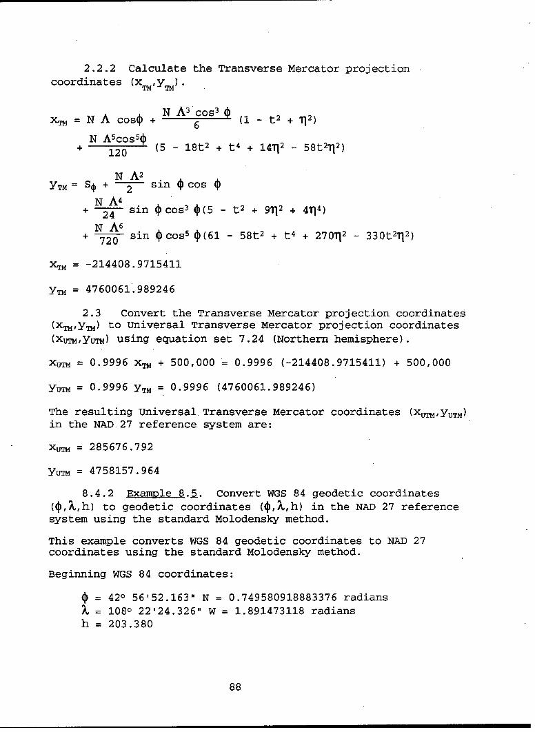
2.2.2 Calculate the Transverse Mercator projectioncoordinates (xTMy T

xTm =N Acos4)+ N A3 cos3 t21 + 112)6

+ 125CS50 (5 - 18t2 + t4+ 14112 -8t 21I2)

N A2y~m so + -2 sin 4cos 4

N 24 sin 4cos3 * (5 -t2 + 9112 + 4114)

N 720 sin 5 *co (61 -58t 2 + t4+ 270T12 -330t

2712)

xTm -214408.9715411

yTm= 4760061.989246

2.3 Convert the Transverse Mercator projection coordinates(x~m,y~m) to universal Transverse Mercator projection coordinates

(XUTM,YUTM) using equation set 7.24 (Northern hemisphere) .

xum= 0.9996 x~m + 500,000 = 0.9996 (-214408.9715411) + 5001000

yuTm = 0.9996 y~m = 0.9996 (4760061.989246)

The resulting Universal, Transverse Mercator coordinates (xUTMYUTM)in the NAD 27 reference system are:

XUTM = 285676.792

YUTM = 4758157.964

8.4.2 Exmle85 Convert WGS 84 geodetic coordinates(4),,h) to geodetic coordinates (OA,,h) in the NAD 27 referencesystem using the standard Molodensky method.

This example converts WGS 84 geodetic coordinates to NAD 27coordinates using the standard Molodensky method.

Beginning WGS 84 coordinates:

4)=420 56'52.16311 N =0.749580918883376 radiansX=1080 22'24.326", W =1.891473118 radians

h =203.380

88

Step 1: Compute Aa, Af, W2, M, N, E2, and e,2 using equation set6.5. Obtain aWGs 84, ANAD 27, fWGS 84, and fNAD27 from Table A.1.

Aa = aWGS 84 - aCLARKE 1866 = -69.4

Af =fWGS 84 fCLARKE 1866 = 3.726463863 X 10-5

82 = 2f - f2 = 0.006694379990

82E82 E 2 0.006739496742

W = 4i - 82 sin 2 o = 0.9984449805

aN RN =: = 6388070.574

a(1 - 82)M W3 6365086.681

Step 2: Compute AO and AX, and Ah using equation set 6.5, andAX, AY, and AZ datum shifts from Appendix B for datum code NAS-A.In this example, the signs of AX, AY, and AZ are reversed fromthose of Appendix B due to the direction of the datum shift (WGS84 to local coordinates).

82 sin4~cos•Aa+A= [(-sinocosXAx - sinosinXy + cos4Az + W +

sinocos4(2N + e' 2Msin 2ý)(1 - f)Af] /[M + h]

AO 0.131,,

[-sinX&x + cosXAy]X {(N + h)cos2]

a(l - f) snfAAh = cosocosXx + cososinXAy + sinOAz - WAa +sin 2f Af

Ah = 28.65 m

Step 3: Compute the NAD 27 geodetic coordinates (O,X,h) fromequation set 6.7 that results in the following valuesl;

89

ONAD 27 = *WGS 84 + AO = 420 56'52.294"N

XND 27 = XWGS 84 + AX= 1080 22' 21. 711"W

hND 27 = HWGS 84 + AH = 232.03 m

8.4.3 8. Convert WGS 84 geodetic coordinates (0,X)WGS 84 to Mercator projection coordinates (x,y).

This example converts WGS 84 geodetic coordinates to Mercatorprojection coordinates within the WGS 84 reference system.Geodetic height (h) is not used in this conversion. The Mercatorprojection central meridian Xo is 2880 = 5.026548246 radians

Beginning WGS 84 coordinates are

OWGS 84 = 420 56' 52.163"N = 0.7495809189 radians

XWGS 84 = 2880 22' 24.326"E = 5.033057346 radians

Step 1: Use equation 7.1 and WGS 84 datum parameters a and ffrom Table A.1 to calculate x.

x = a(% - X) = 6378137(5.033057346 - 5.026548246) = 41569.357

Step 2: Calculate E from f using equation 4.9, then use equation7.2 to calculate y.

E = 42f - f 2 = 0.0818191908426

[t I• 2•> ( 1 - 8 sin • 21 - 5274911.868

y = a ln [tan (+ "2) 1 + 8 sin 0 =)1

The resulting Mercator projection coordinates (x,y) are

x = 41569.357

y = 5274911.868

8.4.4 Example 8.7. Converst Mercator projection coordinates(x,y) in the WGS 84 reference system to WGS 84 geodetic latitudeand longitude (4,X).

90

This example converts WGS 84 Mercator coordinates to WGS 84latitude and longitude.

Beginning Mercator coordinates and central meridian (ko):

x = 41569.3572y = 5274911.8684ko = 2880E = 5.0265482457 radians

Step 1: Compute the longitude (X) using equation 7.4 where a isthe semi-major axis of the WGS 84 ellipsoid listed in Table A.1.

x2- + Xo = 5.0330657221 radians = 2880 22'24.326"E ora710 37, 35.674"W

Step 2: Compute an intermediate value t from equation 7.5.

5274911.8684a_ e 6378137) = .43734619376064

Step 3: Compute an initial value of the geodetic latitude (00)from equation 7.6.

= - 2 arctan(t) = 0.746233651 radians

Step 4: Iterate equation 7.7 until the updated value of 9 issufficiently close to the previous value of *.

82 = 2f - f2 = 0.00669437999013

8 = 0.0818191908426

n1 -r- sin On 2On+1 2 - 2 arctan (t Li +8 sin

= 0.7495688569418636

The geodetic latitude will be given by the last value of 4calculated.

Final 0 = 0.7495809188833704 radians = 420 56' 52.163"N

The resulting WGS 84 geodetic latitude and longitude (O,X) are:

9 420 56' 52.163"N

91

X= 2880 22' 24.326"E or 710 37' 35.674"W

8.4.5 Examole 8.8. Convert Universal Transverse Mercatorcoordinates (XuTm,YuTM) in the NAD 27 reference system to NAD 27geodetic latitude and longitude(', X).

This example converts NAD 27 UTM coordinates to NAD 27geodetic latitude and longitude. The UTM coordinates areconverted to Transverse Mercator projection coordinates. TheTransverse Mercator projection coordinates are then converted toNAD 27 latitude and longitude.

Beginning coordinates areXUTM = 285,677.332YuTM = 4,758,154.856Zone = 19

Step 1: Convert Universal Transverse Mercator coordinates(Xuo,YUTM) to Transverse Mercator coordinates (XTMYTM) usingequation set 7.25.

1XTM 1 0.9996 (Xu• - 500,000) = -214,408.4314

1YTM - 0.9996 YUTM = 4,760,058.8796

Step 2: Convert Transverse Mercator coordinates (XTM,YTM) togeodetic latitude and longitude(O, X).

2.1 Calculate the UTM zone central meridian (X0) usingequation 7.23.

Xo = (6z +.177)(j-8) = 5.078908123303 radians

2.2 Compute the eccentricity (8) and second eccentricity (8')of the Clarke 1866 ellipsoid, the reference ellipsoid for NAD 27,using equation'set 7.9.

E2 = 2f - f2 = 0.6768657997291 X 10-2

82

8.2 1 = 0.6814784945915 X 10-2

2.3 Calculate the subscripted-A terms of equation set 7.9,using 82 calculated in Step 2.1. The subscripted-A terms are usedin the calculation of the footpoint latitude.

92

8 1 2 6 3 64 2 5 p6 175 6 8 0.998305681856A0 6 256 16384

3(214 1586 855A2 = 8:f+2 128 4096 C8= 0.2542555420215 X 10-2

15 3 6 77

A _ _ ( + -8 = 0.2698010542695 X 10

35 ( -41 )A6 - 3072 (8-6 - 88 = 0.3502448582027 X 10-8

315A8 = - 131072 88 = - 0.5044416191579 X 10-11

2.4 Compute the footprint latitude, 0i, using equation 7.10.and a from Table A.1.

Make an initial estimate for 0i:

= M = 0.7463005398433 radiansa

2.5 Calculate So using equation set 7.9 and the estimate of

So = a[A0h - A2 sin 20 + A4 sin 44 - A6 sin 6) + A8 sin 80]

So = 0.4735829138159 X 107

2.6 Calculate S'O using equation set 7.11 and the estimate of

0o 4i.

s'= a[A0 - 2A 2 cos 24 + 4A 4 cos 4ý - 6A 6 cos 64 + 8A8 cos 84]

S'o= 0.6364798134276 X 107

2.7 Find an updated value of the footpoint latitude, 01 usingequation 7.10.

i(updated) = 4i(current) so _ _S = 0.7501073756426 radians

2.8 Iterate Steps 2.5 through 2.7 until successive values of4) are as close as is desired.

93

For this example, the final value of 1i is:

Final• 1 = 0.7501073020563 radians

2.9 Calculate values used in equation set 7.12 usingequation set 7.13.

t, = tan ti = tan (0.7501073020563)

aN, = - 6,388,261.949762

4i - 82 sin2 1i

a (i1- 2)R (, i - 82 sin2 ai ( = 6,365,044.225886

i2 = 8,2 cos 2 1 = 0.3647692467262 X 10-2

B 3 = 1 + 2t, 2 + 112= 2.740138642336

B4 = 5 + 3t, 2 + 1112 - 4TI14 - 9t,21112 = 7.579827062321

B5 = 5 + 28t, 2 + 24t 14 + 61112 + 8t 1

21112 = 47.45050110665

B6 = 61 + 90t 12 + 46111 2 + 45t, 4 - 252t 1

2111 2 - 3 111 4 - 66t 121114 -

90t 14111

2 + 225t 1 41114 = 172.1890097418

2.10 Calculate the geodetic latitude and longitude (•,X)using equation set 7.12.

t 1 Nr~ L X-2 .B4 (X' 4 B6 (X 6101 I R,12 (N ) -24 ~NJ + 720 (NJ)

= 0.74958094314009481 radians = 420 56' 52.168"

=o + sec 0 3( 5( %

S= 5.03305669671 radians= 2880 22' 22.464"

8.4.6 Example 8.9. Convert WGS 84 latitude and longitude(0,k) to Lambert Conformal coordinates (x,y) using two standardparallels.

This example converts WGS 84 latitude and longitude to Lambertconformal projection coordinates in the WGS 84 reference system.

94

Beginning WGS 84 coordinates are

OWGS 84 = 420 56' 52.163"N = 0.749580918883376 radians

•4s 84 = 2880 22' 24.326"E = 5.033065722110382 radians

Standard parallels:

01= 420 30' 00.000"- = 0.7417649320975901 radians

02= 430 00, 00.000"- = 0.7504915783575617 radians

Origin:

•0= 420 30' 00.000- = 0.74.17649320975901 radians

3= 2880 00- 00.000- = 5.026548245743669 radians

'Step 1: Calculate eccentricity E from flattening f.

F = 42f - f = 0.0818191908426

Step 2: Calculate q at 0, 1,02 and 00 using equation set 7.27.

x O I- e sin[= in tan ( + . ( ]

where i = null, 1, 2, 0

q(O) = 0.8270301921136922

q(01) = 0.8164293462094778

q(02) = 0.8282703592274435

q(40) = 0.8164293462094778

Step 3: Calculate N at 01 and 02 using equation set 7.27 and afrom Table A-I.

N (0j) =a1) i92 sin2 i

95

N(OO) = 6387903.46785173

N(02) = 6388090.05758619

Step 4: Calculate L from equation set 7.27.

in(Nlcos•!) - n(N2cos02)L = c 2 - = 0.6788029306559900q2- qi

Step 5: Calculate K from equation set 7.27.

K= N cos - LN cos -= 12076169.25203636L E-LqI L E-1 2

Step 6: Calculate r and ro from equation set 7.27.

r =K-Lq(O) = 6888432.18075871

r0= K-LQ(o) = 6938179.32109766

Step 7: Calculate the Lambert coordinates (x,y) using equationset 7.26.

x = r sin L(X- X0) = 30474.8898082

y = r 0 - r cos L(X - XO0) = 49814.5521555

8.4.7 Examole 8.10. Convery Lambert Conformal projection(with two standard parallels) coordinates (x,y) in the WGS 84reference system to WGS 84 geodetic latitude and longitude (OA).

This example converts WGS 84 Lambert Conformal coordinates toWGS 84 latitude and longitude.

Beginning Lambert Conformal coordinates, standard parallels

(0,,02) and origin (0o,Xo) are

x = 30474.890y = 49814.552

01 = 420 30'00" = 0.7417649320976 radians

02 = 430 00'00" = 0.7504915783576 radians

k = 420 30'00" = 0.7417649320976 radians

Xo = 2880 00-00" = 5.0265482457437 radians

96

Step 1: Compute E, L,r 0ok,NjN 2 ,go,q 1 , and q 2 using equation set7.27. Obtain a from Table A.I.

E = V2f - f2 = 0.0818191908426

qi7= in tan + - - sin inS0.81642946+207+ 7 sin8

qo= 0.8164293462094778

ql = 0.8164293462094778

q2 = 0.8282703592274435

aNi=a1 - E2 sin2 *.

N, = 6387903.467851727

N2 = 6388090.057586191

in (Njcos~1 ) -in (N2cos0 2 )L = 0.6788029306559713q 2 -ql

K Nic=so, N2cs2 = 12076169.25203651Le-IQ - Le-Lq 2-

Step 2: Compute ro using equation set 7.27.

ro= Ke- o= 6938179.321097849

Step 3: Compute r and 0 from equation set 7.29.

0 = arctan x = 4.4240820859501107 x 10-3 radiansro - y

r - c - 6888432.18091526

Step 4: Compute geodetic longitude (%) using equation set 7.28.

L= + Xo = 5.0330657221511255 radians = 2880 22' 24.326,

97

Step 5: Compute q using equation set 7.28.

ln (r)q L - 0.8270301920802524

Step 6: Find an initial approximation (0') for the geodeticlatitude from equation set 7.30.

)' = 2 arctan (eq) - = 0.7462336509266212

Step 7: Compute f(o') and f'(0') from equation set 7.30.

f(W') = -q + I ln LL1-sin4' • + 8 sin ')

f(O') = -4.5493507336696604 x 10-3

f'(4') 1 - e2f (1) = s- 1 2 -')cos' 1.357001593456580

Step 8: Find an updated approximation (4)") for the geodeticlatitude using equation 7.31.

4)" =f(4) - 0.7495861530575

Step 9: Iterate steps 7 and 8 until successive values of 4)" aresufficiently close after many iterations.

Final (4) = 0.74958091885881052 radians = 420 56' 52.163".

The resulting WGS 84 coordinates are:

) = 42° 56' 52.163-

S = 2880 22' 24.326"

8.4.8 Example 8.11. Convert geodetic latitude and longitude(•,A) on the International Ellipsoid to Universal PolarStereographic coordinates (x,y).

This example converts geodetic latitude and longitude to UPSprojection coordinates. Coordinates are computed on theInternational Ellipsoid.

98

Beginning coordinates are

= 870 17' 14.400" S = -1.523451361952464 radians

= 1320 14' 52.303" E = 2.308160619653466 radians

Step 1: Compute the eccentricity (8) of the InternationalEllipsoid using equation set 7.38 and a and b from Table A.I.

82 = 2f - f 2 = 0.0067226700623

8 = 0.08199189022

Step 2: Compute k using equation set 7.38.

£2a 2 (1 - 6)K=] = 12713920.17558161b a + e)

Step 3: Compute r using equation set 7.38.

SKtan (•1 + E sin 10l1r = sin 1 21) 2 303059.087879879

Step 4: Compute UPS coordinates using equations 7.49 and 7.50.

x = 2,000,000 + 0.994 r sin X = 2222991.410

y = 2,000,000 - 0.994 r cos = 1797464.051

8.4.9 E.12. Convert Universal Polar Stereographiccoordinates (XMY) to geodetic latitude and longitude (•,X).

This example converts UPS coordinates calculated on theInternational Ellipsoid to geodetic latitude and longitude on theInternational Ellipsoid.

Beginning UPS coordinates in the Southern hemisphere are

x = 2222991.410

y = 1797464.051

Step 1: Convert Universal Polar Stereographic coordinates(XupsYups) to Polar Stereographic coordinates (Xps,Yps).

99

Xups - 2000000X -s = 0.994 = 224337.434205231

Yus- 2000000YPS = 0.994 = -203758.500100604

Step 2: Compute the longitude (W) from equation 7.39.

I= c + arctan xpsYPs

X= 2.308160619653466 radians = 1320 14'52.303" E

Step 3: Compute k using equation 7.41, and a and b from TableA.I.

2a2 [(1 - ,) E

K = ( = 12713920.17558161

Step 4: Compute q using equation set 7.40.

K I cos •I

q = 3.73652495299514

Step 5: Compute an initial estimate (0.) of the geodetic latitudeusing equation set 7.42.

0= 2 arctan eg - = 1.52313176628106 radians

Step 6:. Compute f(# 0 ) and f' ( 0o) using equation set 7.42.

f()1 -q + L [( + sin • (1- E sin E) • 12 =n - sin 0)(1+ , sin

f(4o) = -0.006730109061328

I - F2f() = 1i - 2sn)os = 20.9875717033244

(I - 82 sin2o) coso

Step 7: Compute an updated geodetic latitude #, using equationset 7.43.

On 0.n-1 - ff' (n-1) = 1.523452437445710

100

Step 8: Iterate steps 6 and 7 until successive values of the

geodetic latitude are sufficiently close.

Final (0) = 1.523451361952464 radians = 870 17' 14.4"S.

The resulting geodetic latitude and longitude (0,%) coordinatesare:

) = 870 17' 14.4"S

S= 1320 14-52.303"E

8.5 List of test points. The test points listed here aretaken from DMA TM 8358.2 (1989) and Snyder (1987).

Mercator

Central Meridian = 1800Ellipsoid = Clarke 1866

) = 350 N

= 750 W (2850 E)

x = 11,688,673.7 my = 4,139,145.6 m

k = 1.2194146

universal Transverse Mercator

Central Meridian = 2850 E (750 W)Ellipsoid = Clarke 1866

4 = 400 30' NS= 730 30' W (2860 30' E)

x = 627,106.5 my = 4,484,124.4 m

k = 0.9997989

Lambert Conformal Conic

Ellipsoid = Clarke 1866Standard parallels = 330 N

= 450 N

Origin: 00 = 230 NXo = 960 W (2640 E)

101

= 350 N= 750 W (2850 E)

x = 1,894,410.9 my = 1,564,649.5 m

k = 0.9970171

Universal Polar Stereographic

Ellipsoid = International

4v= 870 17' 14.400"S= 1320 14' 52.303"E

y = 1,797,464.051 mx = 2,222,991.410 m

102

9. NOTES

9.1 Intended use. This Technical Report provides guidanceon coordinate conversion and datum shifting for a wide range ofArmy mapping, charting, and positioning applications. Guidance isprovided to aid the Army and others in developing software forapplications of datum shifts and other transformations and inimplementing this software in support of operational units.

9.2 Subiect (key word) listing

CartographyChartsCoordinate SystemsDatumsElevationGeodetic SatellitesGeodesyGeodetic CoordinatesGeographic CoordinatesGridsHydrographic SurveyingLatitude

.LongitudeMap ProjectionMappingMapsMC&GMean Sea LevelMilitary StandardsPhotogrammetryProj ect ionsSurveyingTopographic MapsTopographyUTM

103

APPENDIX A

REFERENCE ELLIPSOID PARAMETERS

10. GENERAL

10.1 Scop._ This appendix identifies reference ellipsoids withassociated geometric parameters.

20. APPLICABLE DOCUMENTS.

The ellipsoids and associated parameters are taken from DMATR 8350.2 (Edition 2, Insert 1.) Note: Use semi-major axis a andflattening f to calculate E and E'. Do not use semi-minor axis b,which is a derived geometric constant.

30. GENERAL REQUIREMENTS.

30.1 Application. The ellipsoid furnishes a simple, consistent,and uniform reference system for geodetic coordinates.

Preceding Page Blank 105

44 (Y)

4J(3L 0)()--. 00 00 L ('4 U-~~)

C\JC" C-4 'C14 D '4% (Y)C'-riL. Hr HH r- C)(Nko0

HO1 N LO O ("3-t 000C C O l N O104- y)C V-1~ Cr)0ý m 0T 0 DO 00 0N C) ( Y Y Y l

m ODH )C)Iz Y C)0OD D -ODrO00(nO ODN H H 04 04 00

O~4-)

c) Lr t0 0C r Orr -N(Y)T 1OOO LOHOr-HIzrC)IVrY~-i T r-AL)r N.)m - ( Y)t cc~~l) OOHHO q NU) Dk Y)a I() LO 0 0qw()Or0C - LO

I U)L .OOC)r . . . . . I . . . . . LI L* LOLOLO I-I0H )r to ýw cc L V) -W r-L Da)() clC o- .1rI (

aH N - C a OL )0)- 4rI0 r 0r - 3 c -r -r

Q) _)U)

H

U) (1) 1 LO LO LO t0LO*)() m))1) -W m

H -rIOl LOD t. -W-l.OO aC * - %ot0cHa)m ý ODW -I LOY) ('J wOD to H

C) 110 tO m OOD o- 0) HC- LfD r-OOC ) mm( r . Ol WLrO 0m m-0 W 0 ~)O LO 0- TC N NNmmmNrINNrimNmri- - -Co F -0 -r oO -r -r -r wLO w0C' r- OD 04( 04r 04H

Co in., Mr-r--. r-tr-r-r -r -r r -r -r -r- r-r- *- -r- r- r-- (1

04

H H-

0~ p a)qa)) a) Od w l04 -4XF440W a -

a) _ '4.~ -HU 4.)a)0 ) CIa 0d)I

OD 0 10 00E44-) M

H4 N' - Z -,IC/0 -

a) p 10 )~aOD a U) U)O -)

a)i m) 0

-H -H r- cc) U) coa q~-~0 H) co) Cl) mH~~J43

-H a) a) a) U)4(a a) - ClC2 (1 )

rlU) 0 0 a) S-lH ) C ()-Hi M~~ 0) 4)4 or

-H 4-) r. (d )H r- -W ~ 0C E-1 CO 04H a) > ) OH0 a-- a) 0

H- zCDk 0(344t0 -I CO~( ar-i- H H 4Cl CJ) 4-) 4-) rg1H -O to o l 4-k - Ha-l ) 0r -Hi-Hq-H () Q) a)

a)0) r'1aOa-1aaa Hl 0OD rirA ma15 a) .- ~a -N4 a 0 001u l-4a I L-HH HHHr- -H- 4-)r- HC0 ) r H4-) U)'0'0 5 () a)cl H 0 4 4-J) () MMr) CO (0 -1 4-) r U) CO a) a) 0 .C)-aHHH~)).--Z4)- >)0- a) 0 D - 0Q)(0rA- r 1) Q O r H - r - (1 zd Q 0)C -H - H4 H a)

0)-H a) 4 = 14-4() H> 0 L a) 4 C; ~ 0 0 00) 444ý

APPENDIX B

AX, AY, and AZ DATUM SHIFT PARAMETERS

10. GENERAL

10.1 Scop._ This appendix identifies the ellipsoid center shifttransformation parameters used to transform a local geodetic systemto WGS 84. An identifier, the reference ellipsoid, AX, AY, AZshifts, and the estimated errors (0) in the shifts are listed foreach local geodetic system.

20. APPLICABLE DOCUMENTS.

The datum shift parameters and associated information for eachlocal geodetic system are taken from DMA TR 8350.2 (Second Edition,Insert 1.)

30. GENERAL REQUIREMENTS

30.1 Aoolication. The AX, AY, and AZ shifts are used for datumtransformations using the three-step method discussed in section6.3, and shown by equation sets 6.3 and 6.4.

The following symbology is used in Table B.1.

* WGS 84 minus local geodetic system.

** Derived from non-Dobbler sources, accuracy unknown.

*** Derived from a single Doppler station, accuracy-not verified.

+ See Appendix F to transform Old Hawaiian Datum coordinates onthe International Ellipsoid.

++ Also known as Hito XVIII, 1963.

+++ Use A = 6,377,483.865 meters for the Bessel 1941 Wllipsoid inNamibia.

& Derived from non-satellite sources, accuracy unknown.

107

N m Ln Ln m inin Lm n 'n o in in In)C4IC14 C14CSJ N C~l-4 Cl N l 04 0

qw COto 0 40 n in T-1N r- tO Nn CN 0 r-I r-IOl 0' 04 04 0 C)N m

4)V l C~~~lllq q

14 ininmiLnin n a) 'n o in in inLn C4~ 04 l04 C14 04 - C4 04 Nl

4J

in V 04HO~ 000 OO m %0 G Cl4 m$4 1 r-4 r-nCVI v-I C-4 r- - wW T4 0 i

I I ii -I 04~ N v-I I

OD z

., ( L-; in in cV) n in m) in 'o in in in4J HC 04 N~ 0404 Cl4 04 -I Cl4 Cl Cl4

0to@2 O D Vqin M OD -4 mV 0(Vm in V- 0

V. %01 r- (n %D C-4C-4 Rr in~ Rw -I 01 N-rqsU M -I v-Iv Hv-I-I V-4 -I I v-I tf -I Ro C4

914 'II11 1 1 II

E- HV D 1 3 0 0.g4 Dm 0 %0 93 O

v-o V ) *rl OD to -I OD0 0 > -I i tos v-I

Iq4) fn 0 Id H-434)0 w 9 )c 0 as a

4H $4 co 14 W 14rI .9as aso O' 14 4)JV V 14

U 0 W m 3m: Ho V-I Hi- U q

0'

P4 111 11 1IH H IH H H H HH HH 0 iz 0

E-H H

Ho

H 02

E-1 IK Hd Id4

Hd P4v1r- 0 4)

W*a r-f r4.Iir 0 00 (

0 o > K 0 f ri4 d j r

>fr 4 Ar- -as M 40r -14 0)O

as0- 4) P 0 z (a to.0CO H mVI)U

0 U, L

5m0 1 %T4 01r CDi Clh lC)C Ul'% Cl

4) 1 1 11 11 1 11 1 1

'a)

>1 cnUn o(n R ,ULnri O 0 U, U)

E- m0 Cr4CHC04 N NlN C14

54a, ulL U) 0D U,,(n),1' Ui v ww ,

4)0 1 O r-0IrO 0 0

$44 Z4 i4iI I

gI Go 0 inUUU 0 UOU

00

U)U

o Hn CD 54 54r4R nr-o n04 ax Wa - rIrIr- qqe q rI -

14I >1 r- r-

o- to t

oJ Co OD 0 0C~rzH.) 0rI V II1

01 H -14$4 $

4J1 P4m 93C

E-i H H

ni a, H-

0 0 10 r4rrI 0

to o o

E-1E- 0W H0r * 3 d N d )13t

mI 01Go ODc 0 U) 04 v-I64 C4 H- 40C') m1 r- m0O0) L- m C4lV C14 v-I

4J II<LIn In K n In m'

I4 n 0 Cl4 M' 0 0 In$P4

E-4z

9: 0

.14 00 -o O O

E 0 CD 0 01 M mx M- M' V-I W-1 04 v-I

*E 0

$4 >1 v-I v-I vIuI r -

4o o 0 ~I 0 0 0 I v-

E-1~.1 .14 to( ) oc g 1V 3 w 3 o m 3 W :qw 9 qw $4 $

0 $4 C4 64 N 0) $4C-4 w4C N 4C EU EUd$40 rz) 001 M 00M 0 00m14 m0 00M V-4

.1.,- .Iv4 D4) 4Jv- J- Vv-4 41V1 Vr q U

0 WHPz4

0 0

v-II

- EU

U.

V W ( V-4$4 Id

E-1 rl0 0 *EU$4I 0r W

E-1 EU EU $4r 0CO) m1 Z) .r4 Id IUE

m. 51 0 O)E Pa 0 0) 4) 4) 9r, v-I 9: tm 0 :%l rd 9

1).14 0 EUC E .0 ~ 0 (D tU3 ca~U

co Ln Lc) Ln Y Ln 0 Ln Lnv-I C4 C14 04

to 0 qw I,0 - Nl H-m H C14 1 Ln C14 R LA V-1

4)

$4 Ln m0m LO 0 LA LAv-I C4 Nl 04

4) t

0~ q A,'~ C4 C, Go 0M qwOD N V-4 H

9E E-I

41 C.)LA LA (qI LA 0 LA LA(d 0 -I i-I Cl Cl Cl4

04 0Aq ~ -H) (' Y) n%0 W (Y

$4d C1 X -I '-4 04 Ev) ICl4 Cl NE-1 U) z <

S4.) .)

E44 r H H

o) 100t o r d t14 4 H OD 0 0 0 OD OD c 0 0

0) 0 H- rj *vq *rj v4 I-I Hi *rI H4-) 4 4.) v) v 4.)0r. 04 EU IU to Hd a) 4) Eo to4) (d H M C9 0 4 M A4 r4 rRUJ 0 . $4 $4 $4 "r $4 Ri 0) $4 w w $qw C14C

0 Cd EU) Ro *Cl N N 0) to c EU Cl4 CD MV-I 0 4 ) Cl V)0 M0 4) '-4 v-I 4)1 m 41 r-4*4U C: 0i r~-4 9: -4 1 U H 93

01 H H- H H H0)

H- HP4 H In

E- H

H

44

H Ho0rI0.Hc

FAE- g 9 0)I 0) EU I0 -4U) - I-A Hd 4 H EU

0H go >1v EUH 0 (I)IHEU 4) E0(dc ) Hi4 1I

(l rl NH - E-1 $4~ r. Mr 0 H 4 $40 ' '4l *rI 4)C NC 0 0 ) t 0 $

rU V ) 4 tor r V N0 0):3C d $4 1 iri4) EU

'K 0 0

0)~ H- ri H~~4 -

64

$4 Go ) IACO m m

a) rVd IH

Cl)

u OD E-4 <- I-

0 Cl

.. 0 H.J4.) 0

0

H o V- V1

~4J ,:

E-1 r 4.) f-I

0 H0

144) 04 rl

$4*. H0 ~ ~ IN..

o P4 4) (A93 -I

.1*1 H

. Hr2I 4 Wz P4 x

HHI I II I

WU~ EUf C4 4 1

d *r 4 00'0- $4E 0 r-4$ 0' M

4) to O4) EU 4)s 4 M H 2 @0 $40$ 0 .0 4J @ 0. r- 03I

H *r (P4 U0) 4)0 :3 :3 0-IW 0) 0 4)E-1 M r-4 0 $4 4.)EU~.$ EU (d0)040A I ( 0 c *

rzl 00 a -$4 0 r4Q 12 c &0 s-i H-I ria-4 9 9 H0)Kr 0 '0 44 01 0 11) *0$4 0 0 140.e4H M4 4) w to tou)

0o Z 9 ~ 0 (A %H V 04004)$4VP4 ) 20 -0 0) 4 H A HWz $z1 0 r. D-l4c t4: H U .

C0E-. CO U) 4UJE Pl4)MV c *E41 vCa r-4 cUJM -H (D4.) r-l s '4 0) . 1ri -l -rl 93$ %r

>4 ( vrq$44) -I $4u- rq % 4 04. 4 Ur.W :IdCC- gca >$4 IdU.Q 0 CC >10) r4 V$4 .ri 0$4 Id0 CO ) C 2 I 4r, .HH

14 (d:3 4)$4 A.rl4.)4) 0 04 r Mt44)4)0)0 4) 3 00 C'U

PCL 4W 9

U- U K i ) m m VU') U) (T) U') Ur) U-)CJ, -IK CN C14 C4 C14 C14 N

o r -I o inoo~lf 01 U)(An 0 M1m 9. q' w 0 mC1 qq Ro ej'04 W) 0H) T-4r~- H - -I -rq ,-I H -I C14 04

$4

4)u <

U) $4 ko M)~I CD U)IýCD O U) N-$4') 1~~0 I 019ICJ CtoD' w4 (71 mr~- i-4 0 iI I0 M Cl ODr IN

0) od 4 - I rqrI I I I IqI 11C V

.10

41 HCl)~

r - 0 ) 1w 4 1 1 ~ ~ IIP

OD ~' r4r II M IA D D -I OD v41 4 I - rI I rI

E-4

44)r

0) HG0 0 0

$4 4) ca 4d 44) H a,34)9

a, 1 $4 V~ $4 "Wj ~e

4)1 (% 4) 001 4)1Mo g3 T4 1-f ny-I 93 -I

HUH H

0'

04 H H P5 1111 E1

D C CD) 0

E-4-

04)

H u--' ~ ~ $id 414q

0 0 W -. 161 0 :0 V 0E-4 13 0 > >1 -ICl 121 Cd z) I

C:I W4 E- H Vcd.r0)d cdý 16a ý Dr

W6 t-) 1 a) 4) .0) 0 Cd 0P )rI -$4 H~ 93 ICld I 4H Q co

w , , Id I v-116v4r- $4 Cl HH 0 c H416ri IUd 1 go d r$4 4 r I

"I -H 93> 111 4 >$4 4) N .. 4 -I Ha,)0 U -.vri H d 3Id t 41 A .ri 41 A)1 E-o m

a,)b 4r169v4d4)0)'r4 :00-m ~04j (dri *v 04) d ( :3$4 $0$4 $4 ri 3 Id: 1 a,4) Ill 2 04

$4 4 4 d ri 0 :3 4)04z l)Cl) Wa) a) ) a,4OHH ca W z 04 Zi A rl

M C14 04 Cl

co 0% i-I TA 01 %0 l (

0) IV 9) V4 (D "V 10

44 $4 1-G 0I M

0) Nu oC4 %0 C4 N NV LA I

a. [P4KC

4J 0V C14 0lI4 01I

O04 > 0 Ln mD 0l C cqE- U I I I I

o )

0)

to Vo tolt CV) go) IdI

04 %0 Rr 0 0 0 LA 0V A$z 14 0- Ci Go) OD H 0lrj r

d II o Id Id Icc4 $4VM- -0 4R 4RV $ o $E4 034 0)C4$ "4 4 - )N 0C4 a4 "4

$ 0 0J M o 04 0% 40 0 01( 1h 4 01

H a'H"4

P* E-4 113 "4 ~ 4 ~ "

F4

~34 4

Go 0 0

-F 4$4

H I E-UIE-1 ~ 0E 4) IU "4r-

P4 W 0) $ M 0 1)Q CO 0m.40 H4

Ma IZN V n"

C) 0) $4W EU EUo3 ri _ 4)4) 0 tl cn r,- 4)0M E-1go 0)U-

ca $4D: w0) w ) r, 4) 0U r

0J 4J rOV H7 EU3 "4 d d W o

0) 4 rl EUr

- aoH- -

a) eAL Cl mA r IA RrL m (V(364N -4 C4 CV) ml NC Nl N

4)

$4 inII C E ' l lC

V, E- tDN NIIC404) r

a ) (d N V o H-- - 4r

E--

0 to ri <- I- 04 NII 1

o0) ca

44v. i-i II II u

~4) >1

4.).~ w C-I l W-1 r--I r-I rl LA 4.)

4)J~ I)I d t d 0 dc d4 j0S

0 - 4 V 0r 0 $ ' 41 - l0C4 4

o0 P4 oW00 4)0 0 0 0 1 04 1(Hr > 'L > ' > ' > ') 0 Q- : -

a0 04 N0 wI P4 *rH

a) 9.,I v1 v4v4r 1)4

aU H M)EU(U 0)(UP4 )ED M) Z ED E-0

o H H__ H H H H

*1*4

rzl

U. E CUH ~ 4) r4 (d

E-4 4) c -4) riIP-4 K r- L 0$4 *r4

0 o%0 r4 H~ 0 r (U (U 0 $4P(U A o o 10 .ri y-I 93 a, (d

0ED I V(U $4)9 v-4 rq u '0$4 00 0to d I (U 4)U IU 4) 04)V14 H o F4 9 1U 1 I 0 c

~C/Ifllq r 4 a' > i4 0 ~r4 4) 41( a, O

10 Id ,9 J A Q- 0 C0 a ~$4 0 00w *rjEz m CH H z> zH H Z cn H

H- H

<I oO It 'a W n tn ul Cl410 CY 04 C14 CY H

EU0 % 0 i-I r4qV$4 < C4 w V-4 1-4

o

$4 0 In In N n V-

-. 0 H q N

.1.) $40)wrl i 4 r- OD Go n r- N *

o to z -

4) 0 In In in cqLIn 0 In 1-I C14 C*l H-

~44 04-4l 0 0

~ U ) H 0Ln m40 V(CIO S>, 10 1 )I

to I < y-I I -

E-1 rii o.0 CUD0 0

to 1 )0 a$40 0 0 0uI0 O OD0c; 0 *rj vi4 -I - II

4.) W) o)4 )E04 (U 4) to 0)0

.0)U H 0) 0 Ad.1lu 14 $4q v 0 $4 4w $40 Oq' 4) $4 1~4

044) N 004 ) (n 41N ) q0) o C-4 to I.H 93r1 -4 r.- au-I FA u-4 iI

0)

HE- 0 U)PEz U 1 0

Q Id

U m rE 0

El H) to C.r 0

r.)> H CD toU' 100 m cc 04).rI $4

rr0) 1H *r-I $4 41 m m0~ r" EUEM 00 g 40 E0 4) >~1 z04 ri a r 9

to :3 rd ( r-I 0 cc $4 CA rj $4 0)' 00 $ $4a A0~ ~~UU $4 4OUi ( 4 i c

M 0% in in un (Y n in Ln inN1 N1 N C1 N 04

'-4 N~ Ro 0 r- r inNc in-% n , m~ q0 N V-4 N %0()I I V-4 N i-Elr-I C")

$4 <

$4 4 i-I in in n C") m in Ln w in0- N 1 N N N1 Nl N4

4J $41 m 0 0 in Go qw~ m O(r, to N N N4 0 iw n OD in

0 I4 N4 1' 1 4 w I I I m"

41~ 2: UO n in i n in in i n inC in

go 0 t" C') '4 04 C14 N i4N C4

~4.4 ulr.

M0 AV) n 0 m. 0 r- 0 D 0% r$4 >1 H *1x

E-4O

44r4I ~ ,a .4 a - )4.HE HJ M 1 4

4)0 ic 4 0) $ ) 4$0 0 EUEU 0) E . EU EU

'.4 0- 0 -I V-4 4-4C r-I -.14 N) C)93) )C

to H $4

f-I rzi -- I II

00K

a),Al,

H z1 EU z1

.14.1 0 r4 K H 14'

E) r4~E 0U$$ 4)~

0 00) d o

L n Ln o U, m '

04 Nl OCr14 N f '0 U

4)% o r- to r% rl-

4) <

0) H < C4 C' C14 C14 1-I

4) $4 0o W~~ N ) 0

0 Q~ Z < -I rI-44 (Y C) "4i "4Go FAIIl

oU)

t-Oj 0

PC C-4 N N N

rEU) - - 40R4q0 43

$40 >1E

0) 4.)

* H 6 4~ V A4J ~ $4 $4 4)C14 $4

0H0"to4

124 H

0-0) '009) U) (dE0 0) (d (d 0 Eu

0 4.) 10$4 9)EuMi -)-(d E4) 01 UO() t E 0 C: M~ -H r 19

E-4 8 w z )ul o014 o 4 0' 41*rI 0 00 mU E-4 10 ,-I t

0 0 o- W) tEu 0) X 4J 0 4,)ld~ Izi H 10 41 Id u z4)0 0,4

r I "4Q DC 0 *rl -- rIO ZM W .WUl) 0)E. Id ( 0 C: Eu93H Eu u u0u-

H. Id :3 93 4 Eu -0 01in Ctl30-) V 1 K 0 0 r g 0 r

0 -rl4J '0 r. r $41 Id 10 0 4) 0 041

0,(d (dr rd 4 4)V0 0JzQ M0-4 U) r Eu 2HH'ZO)

___ z0z

$4a) 0.4M l

-14

E-1_ _ _ _ _ _ _ _ _ _ _ _ __ _ _ _ _ _ _ _ _ _ _ _ _ _

14-

4))

0 04 1 E) r4C

u CD

0 C1

0 - ) D4J~ 0-

44 C) C14C14

141

0 04

0

a0 >.DC04

a) 1 5 z

OHz H

0 o : 4) -- lg 4) 15 *r)4) 4J U(dM 1 4) Mr 14) 0$d.H4) 44

(n0 r.0 $493:3-r Mr 0 -ri *I v)0VE-1 C:I4M 0 -14)C M 40~ 4) -l .a4) m 0 PI Wto

I'4)U*.rM Wr02 )HM .C15or.4 cJ15. .*r0. 1a)- Z - IZ0J a) 4) oa)

E- 4)qId4)14C :'rdov 0:rf -0 0 (d4 >- w o0 ' 44

C/I A 0 t -Im -I l 5r-I -1i-lM4) - ;4 i3 .C4) W*. -4J000 id co 4W -ri ->, w m0* s 9 02 Id ~ r.to x : m

M 4 4 04)ro0 (d-1Wr-14) ) (d ). -A 4)4)

0 cz pa- u-~

() 0 Cl40 ~Cl

0) 0o Goqo Go Go 4 0 U') %0

41 tIr-I r4I r4I r-r4 H V-1 Clg r-'

N 04

i-4 Cl C

0) in u,) 0 C-4~ On ') 040 U

.4J 14I94U U -

o 0,Go U) C D W)f (n a n o Lfl U') 0

0r Cl) C

0 M~ClO r- o 0-

5441

too

44) 0U)V H A

0 ..4 1.4

4J U

0 Hrza 0: H - 0 0

01 E-0) z

u-Id

-p 1 91ccIr-4 0 00 4) a

I'- 0 9 0) (D ul 5.4 4 Ol 3 c

U 04 :j: -H. zU IdV EU: 0 IdH M .- 40 .&1 EU ) 4~J 9: -ri4 C -4 EOd

V- ( EU v4 -ri9 -.riE VU 0v Edm COi.) *0;> 54 0 0 -$4 :: ~ r4 H 0 M , %

0 EU z. W Od 1 )00H $4 1 U 0P4 EU coI -V0 E -4-4- 4E') K 0 0) VEIdCDE-1 H 1 0b Im a V E EU vi a MI5C 4 rV 0-U 2

V) - m 0 0 .0 4-) W 93 0 EU U 0 tAO>4 4 -)9 :3 -*ri4) EU 0)@ 0 v N H$4IdE

0 10EUv (d04&0)00 EU EU EU('d q 0 c - -I -AId EU

0 U 10 -4E5. 0 "'- X U)4 I - $ ) 9(d EUr- 4) r- 4~J 4):V ri 4-V00co4)M -i0Ha a w.0 0 (Az $4~g. 93 9U) w 3m r 3 0_4A0 -p1HH riu cc mEU EU0E EU EU EUCd c 0u. 09 Pl x z >4 u ) U U

N -O

if) 'A %o if lncqc,4cl4 c,4 C

N N 00

W4 m ~ r- i 0% V< co H H H 0 OO

a)

01t in Cl %D C4 C. C40 C4 Ln

H

04 RW 0 0 0 00 04-) V' i-I ('1

0 0$4 In ____GO________c,4__o4_c,4_c_4

Go

4.) -

$4 >1

H OD0 OD

0 14: CD 1

4.) C

0 Wu

01 H

*rP4

rzi

- uH

0) Id I 0r )I D r

H) jig)V $4P4 CO E4 0)r

0 H 0 m a m0 0 Hd tHH

:30U0C.) E)$4 IK Ew to VEU Ufo Eu- -rl01___r : rrEu EI a) 0 M-j 41*0 o lu $4 $40H .i.QuvI Eu 0E *u4 E-1 ru. u> a

A ~ ~ ~ a 0 d. A4 om a)A 8X NA 0ro~C 0 4 o : $ - p -Im c () r

<C-4 CotOU oOn L U') W Ou 0

CC4 C-4C-4 N- H. H -I

(Y) '.-4 M N R 'I 1 ul$4 (1' (1)-I' coc r o Nm41) 1 ri '.4H C- rI qw IV Ro N

41)

N. U-I N'4.40H

$4 /4J Dr-4 00 101 OY 1 V v-I C4'. W-1

) :H4 r-I N-N C CC4C4N 04 vi .4I u-IE-4 < I1 1 1I Iz

4~$4 I-

(n fLn )LOnt)OCr) 0 10 0H to

0 )NC4CN 4 N r4 v-I V-1

~4J It 0 vVUU WI ' -14 qeI0o % OD Re %0) UDL)q IV '.'- co

44. i- V n) ()I (n)I

C34. - -1to$4 >Ir' +

toI4J H 0 M G

1~44 rI 0 ri u-I CDC

0 41) 04 co.caV H 0$4

0o $4q V 4)$441 A 4) -4 $4 $4 >

4)4 7 -i Id rd $44. 9 -I 411 i-I v-I

ru-4 _ _ H Cl )

0I

014 [z .

.rzw 0 000000[e 0 0 00 0

z- H-

r-I ~ 0 0 .

H4 4)- r.ICJ % 00z $4 P - H a

0 0$ rz- C6I m 00 v-C 4) X 0)

vUO EU I-ri > U0EId IdUEUV9

0 0 0 C 1 to go-HI :34)V -I r-f 41 Id

04g P . 30:0I4 a9 EUEEUUE (U E 0).m 1~0 0

4c

to r- C-4 I) w-4 qw en)$4 m~ 04 C qw %1 CAI m

4)

0 U') U) It) I) In U'E-4 04 Cl C C4 Cl Cl 04 04

4) Hl U' 0Ir 01

E1I I

O0 N 0 In It) U) U) IA U)

0 )04 N~ U04 CW 04 04

0) (a 011

r41o

o- OD 0 W a -0I C H ri *r4 U)I U)I -Ri

$44q >1q go I4Q to

4 O HC rj Cl ODl OD r544 0.I5 4.)0 4-)0 UE 4-)01 4

Ul V$4 4 w-RV v-I -4 $4- I1-

H) a U HI-4J U

0

o P4 4 (0C)1Co m4 m~ z! E-4 E-1 4

E10 0 04 E- 4 E-4 04

4.)4

144 Co64 OD

E-4 14C *.4 .-4.102 row

0~~~~~- HdE1C j - rw l i -I H z 4J %H EU

U 11E $440 ) c

E- Id 0 3 4 *0 :4) toE HO0 0 Id

r-q n 0 IAnU m 4Wc4 )n c 0 04Nl 04-I 04 Clq i- W4-4 Cl "1 4

- .0 0o 0 Nl H-I r (1 0%-I i-Ir, GO 01 qw rww i- r- 0 C14 0i

M4 M IV CV) M7 Mi M m V) 1 -4 OD

4)

020

I'- 0- L 0 qe 1 =Lfln r vro-w 0 C')E- C- vIC4 014 r- C-4 04

.J414. r, Go OD qw Wn r- LC)ooo P, .O

o- r- -4)I 4 V4q' q -

r0( c)4 0n 0 0 wn Cl 0 in MH 04 fR0 0I)'O1 14

OD CI 04 I -11 1 Iu Clj 04C 7 ll~~~ -

4J~~~ ~ ~ OD0 0 0 m0II o 40 02 Gor , D-I( - C- %0

$4-) 04N04 (I 0 40 -

00

00% 0 04.) 04 rlO l r

04 r 0 40 4.IJ .I1~

E-4 D -4tr A g

U) 0

H4 C).)1~C

D44I I I 1 1 1

02 1-1 040 0440 t0ýE-04 04 04a k da a

1-i

$4 **

I0 a4 K$4 '44

M -4 '4to(D (H "1 .140 C: 9- 90

tol 0 : D aL)c r 0

rz~z I 0D:

.. O 414) 0 N( 0 $4 a:3 IL) , 4 $4 v1$4 40 10 '.4 r .l 4) 4)

a- 49 ) a) .v4 $4 ) H g 04 $40-) go4~4 0 r 0 0 a N 02 0

in -I I 0 0 0 0 0 w 0 41 a $4 014C

GU W go 0 U pa 04 Ck :30) I 0004i

m 04 mm -,0 4

'4 Uw , co) U) Uin r, In w

U) N 04 1' 10 N -

U) NNuj

E- ~N N 04 04 N 04

H

5,4 -o

41 %' D N Ný v01 N

(d U

OD a) LO N U')L U) -I 0 It)H 04 N 04 - 04 04

EUH - 1qL01 N Go 0 0 t u- 0

C%4 U') u-I N 04 I

o4 I1t Id Io Id

MElU CO 4 ur -I r

4)0 0 0 0 >10 0 0 .q' 04) U H ri -4 m 0o *.i *4 -1l 0D -

44o 41 41 a) '-I 41 41 4.) ''-4 4)QD ,-4 04 - V 0V-I C

ca V H $4 $4 ) 0 54 $4 $4 0) $40 w' 0q' 0)0 0)m 0' 40" 0' 40 m 1)

50) 0 C4) 4)N 04 0 0) .9) N 0 N 4J N 0) 4.) 0(D ED 93 0 M 540 0% ) 9 al ~0 9 ~0% 0 C: m

0) H v-I H u-4 H,- rH-4 H -4 H4 T-1u-

0

0 H014 zU1

H

*14

Id Id

-.4 K.-4 EUdN C4 Ad ) EU u-I

* H V EU EU C H V)- 910 .4 01 4m> n 3 H 0

EU $4 r '-4 0 %D0 IdW VIdI EUU-I M4.) co5 w V*

0 '.4 0 V) u-I 9 0 EUW H 0) >,N t

* ~0)H 0 - O r-4I '.4

co Ip 4) 0 ' 4H pw( c 4104 0 -A.. 0 rj r, . W4i O

HC 0 V-rI l A 0 rj4 Id~0 EU) 0l5)$ ý4 r. 1E4 0*rIV m Ia

0U NJ E03 4) (d m -dI

9C 0l IdO w E 40Hz c

W L L U LfULfl U, mV U ,Ln UCV)n U) ta<C.Jw4 r- -4r 1-4 04 04

r- 04 o .- I~' 40 r-CVM'q'CVen m$1~ ~~~ I I I1 1 1 I 1 1

CD

I'J- l Id C4zx

0i 04 1- Hr- 4 04 qE44 U 3IC

4J$ z

o04~Hj C:iI iI dC

0) U

0. .. 1J=-0 , 0 CV$-0 U r-I4J0 I 1 1 1 1

$44 l 0 4 4

4), 04 Ar~gCOV H .04m440 $4w

0 A 4.)O Mr6 4)c0$4 0, i-I 0.s N 9 O-a, 1 O 0i ~H

E-1u

.F.I -I I 41

01 H4 Id H0%mCU2 0 0 >IA :H. U)) U))UU))U U) U))oUU U) 0)

'-I1

Hd H d H d

0 $ $4 K)11

cn0 i 0 40 goI0 >4)r- $-Eu, 99 O d c H M6 Eu

U o (d A - - i do>w d I 3 3 1> >~-d u 623.- d- - 00 1 -i4 1

0 r 0 d C 9: 4 -l 4 *0to 0 0 0 -0 -* ri 1rl* 4 J r NrI d -01 $4u $4 i93 W 4 1 d

(d Eu 0 0 49 lrI - dHirI 3I Eu40(P MUCDE- dH Eu (d0$ H600 0C 4 -2o~~~~C V4)4~,% O 2

0 0 0~ OD ) InU () m n KDN r4I 04 C1 04 C-4 N '

OD ui u) r-w to Ch Mo0 a r- OOD OD ODr 0 ,-4C' (Y) (n m L

4I)a,_ _ _ _ _ _ _ _ _ _ _ _ _ __1_ _ _ _ _ _ _ _ _ _ _ _ _ _ _ _

44 04 04 N-4

H-$4 aa, M) r, r- r- OD %D -4 N r- W-I 0

43 % 0 000 CV) 00% in U') ts N*

.I $4 _ _ _ _ _ _ _ _ _ _ _ _ _ _ _ _

0 0 0u 0D0 ODO 0 Ln It) iLf c') U') iKn

0 0 1N N40 N NN1 NK0U H t

H o NDWOD 0 (V) v-f N %D U') it41RW R qi ~~Lf (n N LO 0 r- it' W

0V-4 v-Yr -I T-4 N1 v-I CN

I- m

$4uU I-I H H

.9g. 140 r 0 0 01 r. r

E-4 r 4 0 v-I 43 - r-Ir 4.) 4J. 4.)U) ) EuI 0u Eu

0 H a) a, 14 M 1 $ 4 $4$4 a, D : $4 0)0) aW w Ol$ 4) aqw 4)q' 0 aqw0) CD a1 a, 4J 4N IISd Cd : 4.)NC4 4JNC -

4.)a P4 > )0m H- - 0 93 Mr, rqH r-IU00 m H v-I H -I HiV-I

00

'pj >1 > 4 1t

H- I I

44H

(d IV N3 m

in *M w dI dK

0d 0u Eu0 %D U) r

Fzl ri$ cc $4 xV -IHa) Eu1U)u > u 0 0 U)V Hd t H "O~A HE 0 4ZU) 4u.) Ha, 41

0 d0 14: 0 -ri U) HOul U)

k d( o13c U bU 0 w HH-lr, ( d 14 :mu0 Er4 >EIlr $4

$4E>

APPENDIX C

DATUM LIST

10. GENERAL

10.1 Scone. This appendix consists of a list of countries andgeographic areas and their associated datums.

20. APPLICABLE DOCUMENTS.

This section is not applicable to this appendix.

30. GENERAL REQUIREMENTS

30.1 Apl. The intended use of this appendix is to establish atable of countries or geographic areas for quick reference to theirrespective datum.

129

TABLE C-I

Countries and Their Associated Datums

COUNTRY/GEOGRAPHIC AREA DAT

Afganistan Herat North

Alaska North American 1927, 1983

Alberta North American 1927, 1983

Antigua Antigua Island Astro 1943

North American 1927

Argentina Campo Inchauspe,

South American 1969

Ascension Island Ascension Island 1958

Australia Australian Geodetic 1966, 1984

Austria European 1950, 1979

Bahama Islands Cape Canaveral,

North American 1927

Bahrain Island Ain el ABD 1970

Baltra, Galapagos South American 1969

Islands

Bangladesh Indian

Barbados North American 1927

Barbuda North American 1927

TABLE C-I (cont'd)

Countries and Their Associated Datums

COUNTRY/GEOGRAPHIC AREA DAT

Belgium European 1950

Belize North American 1927

Bolivia Provisional South American 1956,

South American 1969Botswana ARC 1950

Brazil Corrego Alegre,

South American 1969British Columbia North American 1927, 1983

Brunei Timbalai 1948

Burkina Faso Adindan

Point 58

Burundi ARC 1950

Caicos Islands North American 1927

Cameroon Adindan

Minna

Canada North American 1927, 1983

Canal Zone North American 1927

Canary Islands Pico de Las Nieves

TABLE C-I (cont'd)

Countries and Their Associated Datums

COUNTRY/GEOGRAPHIC AREA DATUM

Caribbean North American 1927

Caroline Islands Kusaie Astro 1951

Cayman Brac Island L.C. 5 Astro 1961

Central America North American 1927, 1983

Chatham Island Chatham Island Astro 1971

Chile Provisional South American 1956,

South American 1969, PS Chile 1963

Cocos Island Anna 1 Astro 1965

Colombia Bogota Observatory,

South American 1969

Congo Point Noire 1948

CONUS North American 1927, 1983

Corvo Island (Azores) Observatorio Meteorologico 1939

Costa Rica North American 1927

Cuba North American 1927

Cyprus European 1950

TABLE C-1 (cont'd)

Countries and Their Associated Datums

COUNTRY/GEOGRAPHIC AREA DATUM

Denmark European 1950

Diego Garcia ISTS 073 Astro 1969

Djibouti Aybella Lighthouse

Dominican Republic North American 1927, 1983

East Canada North American 1927, 1983

East Falkland Island Sapper Hill 1943

Easter Island Easter Island 1967

Eastern United States North American 1927, 1983

Ecuador Provisional South American.1956South American 1969

Eftate Island Bellevue (IGN)

Egypt European 1950Old Egyptian

El Salvador North American 1927, 1983

England European 1950, Ordnance Surveyof Great Britain 1936

Erromango Island Bellevue (IGN)

TABLE C-1 (cont'd)

Countries and Their Associated Datums

.COUNTRY/GEOGRAPHIC AREA DATUM

Eritrea Massawa

Espirito Santo Island Santo (DOS) 1965

Ethiopia Adindan

Faial Island (Azores) Graciosa Base SW 1948

Federal Republic of European 1950

Germany (before 1990)

Federal States of Kusaie 1951

Micronesia

Finland European 1950, 1979

Flores Island (Azores) Observatorio Meteorologico 1939

Florida Cape Canaveral

North American 1927, 1983

France European 1950

Gabon M'poraloko

Ghana Leigon

Gibraltar European 1950

TABLE C-1 (cont'd)

Countries and Their Associated Datums

COUNTRY/GEOGRAPHIC AREA DAT

Gizo Island (NewGeoria Islands) DOS 1968

Graciosa Island Graciosa Base SW

Grand Canyon North American 1950

Greece European 1950

Greenland (Hayes North American 1927

Peninsula)

Guadacanal Island Gux 1 Astro

Guam Guam 1963

Guatemala North American 1927, 1983

Guinea-Bissau Bissau

Guinea Dabola

Guyana Provisional South American 1956

South American 1969

Hawaii Old Hawaiian

North American 1983

Honduras North American 1927, 1983

TABLE C-1 (cont'd)

Countries and Their Associated Datums

COUNTRY/GEOGRAPHIC AREA DAT

Hong Kong Hong Kong 1963

Iceland Hjorsey 1955

India Indian

Iran European 1950

Iraq European 1950

Ireland European 1950, Ireland 1965

Isle of Man Ordnance Survey of Great Britain1936

Israel European 1950

Italy European 1950

Iwo Jima Astro Beacon "E"

Jamaica North American 1927

Japan Tokyo

Johnston Island Johnston Island 1961

Jordan European 1950

Kalimantan Island Gunung Segara(Indonesia)

TABLE C-1 (cont'd)Countries and Their Associated Datums

COUNTRY/GEOGRAPHIC AR•E DATU

Kauai Old Hawaiian

North American 1983

Kenya Arc 1960

Kerguelen Island Kerguelen Island 1949

Korea Tokyo

Kuwait European 1950

Lebanon European 1950

Leeward Islands Fort Thomas 1955

Antigua Island Astro 1943Montserrat Island Astro 1958

Liberia Liberia 1964

Luxembourg European 1950

Madagascar Tananarive Observatory

Madeira Islands Porto Santo 1936

Mahe Island Mahe 1971

Malawi Arc 1950

TABLE C-i (cont'd)

Countries and Their Associated Datums

COUNTRY/GEOGRAPHIC AREA DAT

Malaysia Timbalai 1948

Maldives, Republic of Gan

Mali Adindan

Malta European 1950

Manitoba North American 1927, 1983

Marcus Islands Astronomic Station 1952

Marshall Islands Wake Eniwetok 1960

Mascarene Island Reunion

Masirah Island Nahrwan

(Oman)

Maui Old Hawaiian

North American 1983

Mexico North American 1927, 1983

Micronesia Kusaie 1951

Midway Island Midway Astro 1961

Mindanao Island Luzon

TABLE C-1 (cont'd)

Countries and Their Associated Datums

COUNTRY/GEOGRAPHIC AREA DAT

Montserrat Montserrat Island Astro 1958

Morocco Merchich

Namibia Schwarzeck

Nepal Indian

Netherlands European 1950, 1979

Nevis Fort Thomas 1955

New Brunswick North American 1927, 1983

New Foundland North American 1927, 1983

New Zealand Geodetic Datum 1949

Nicaragua North American 1927

Niger Point 58

Nigeria Minna

Northern Ireland Ireland 1965

Northwest Territories North American 1927, 1983

Norway European 1950, 1979

TABLE C-1 (cont'd)

Countries and Their Associated Datums

COUNTRY/GEOGRAPHIC AREIA DAT

Nova Scotia North American 1927, 1983

Oahu Old Hawaiian

North American 1983

Okinawa Tokyo

Oman Oman

Ontario North American 1927, 1983

Paraguay Chua Astro, South American 1969

Peru Provisional South American 1956,

South American 1969Philippines Luzon

Phoenix Islands Canton Astro 1966

Pico Island (Azores) Graciosa Base SW

Pitcairn Island Pitcairn Astro 1967

Porto Santo Island Porto Santo 1936

Portugal European 1950

Puerto Rico Puerto Rico

TABLE C-i (cont'd)

Countries and Their Associated Datums

COUNTRY/GEOGRAPHIC ARE DAT

Qatar Qatar National

Quebec North American 1927, 1983

Salvage Islands Selvagem Grade 1938

San Salvador Island North American 1927

Santa Maria Islands Sao Braz

(Azores)

Sao Jorge (Azores) Graciosa Base SW

Sao Miguel Island Sao Braz

Sarawak and Sabah Timbalai 1948

Sardinia European 1950, .Rome 1940

Saskatchewan North American 1927, 1983

Saudi Arabia Ain El Abd 1970, European 1950,

Nahrwan

Scotland European 1950, Ordnance Survey of

Great Britain 1936

Senegal Adindan

Shetland Islands European 1950, Ordnance Survey of

Great Britain 1936

TABLE C-i (cont'd)

Countries and Their Associated Datums

COUNTRY/GEOGRAPHIC AREA DATUM

Sicily European 1950

Singapore Kertau 1948, South Asia

Somalia Afgooye

South Africa Cape

South Chile Provisional South Chilean 1963

South Geogia Islands ISTS Astro 1968

South Greenland Qornoq

Spain European 1950, 1979

Sri Lanka Kandawala

St. Helena Island Astro Dos 71/4

St. Kitts Fort Thomas 1955

Sudan Adindan

Sumatra Island Djakarta (Botavia)

(Indonesia)

Surinam Zanderij

Swaziland Arc 1950

TABLE C-1 (cont'd)

Countries and Their Associated Datums

COUNTRY/GEOGRAPHIC AREA DAT

Sweden European 1950, 1979

Switzerland European 1950, 1979

Syria European 1950, 1979

Taiwan Hu-Tzu-Shan

Tanzania Arc 1960

Tasmania Island Australian Geodetic 1966, 1984

Terceira Islands Graciosa Base SW

(Azores)

Tern Island Astro/Tern Island (Frig) 1961

Thailand Indian

Trinidad and Tobago Naparima, BWI; South American 1969

Tristan da Cunha Tristan Astro

Tunisia Carthage

Turk and Caicos North American 1927Islands

United Arab Emirates Nahrwan

Uruguay Yacare

TABLE C-1 (cont'd)

Countries and Their Associated Datums

COUNTRY/QEOGRAPHIC AREA

Venezuela Provisional South American 1956,South American 1969

Vietnam Indian

Virgin Islands Puerto Rico

Viti Levu Island Indian(Fiji Island)

Wales Ordnance Survey ofGreat Britain 1936

Wake Atoll Wake Island Astro 1952

Western Europe European 1950

West Malaysia Kertau 1948

Western United States North American 1927, 1983

Yukon North American 1927, 1983

Zaire Arc 1950

Zambia Arc 1950

Zimbabwe Arc 1950

APPENDIX D

WFS 84 Geoid Separation Computation

10.0 GENERAL.

10.1 Scope. This appendix provides the bilinear method forinterpolating geoid separation and WGS 84 Geoid Separations on a100 x 100 grid. These separations are expressed in meters.

20. APPLICABLE DOCUMENTS.

This section is not applicable to this appendix.

30. GENERAL REQUIREMENTS.

30.1 The Bilinear Interpolation Method of Calculating WGS 84Geoid Separation (Nm•_mj. The bilinear interpolation method usesinterpolation in two directions (0,%) to approximate the geoidseparation N. from four known WGS 84 geoid separations givenin a look-up table. The bi-linear interpolation method has theform given in equation set D.1. Figure D.1 shows the relationshipbetween the positions of the known NWGs 84 values and theinterpolation point.

Np(4,•) = a 0 + ajX + a 2 Y + a 3XY (D.1)

Where

NP(0,1) = Geoid Separation (N) to be interpolated at Point

a 0 = N,

a, = N 2 - N1

a 2 =N 4 - N,

a 3 = N1 + N 3 - N 2 - N 4

x= (0 - )(02 - 01)

145

= Geodetic latitude of Point PX = Geodetic longitude of Point P

N1 , N2 , N3 , N4 = Known geoid heights at grid points used in theinterpolation process.

N(( 0)Ns( •N4,0) N( 0 , X2

N(Or X)

N2(01, X2

Figure F-I Coordinate System Associated withGeoid Seperation Bi-Linear Interpolation Method

30.2 NwGS e4 Tables. NwGs 84 values are tabulated on a 10' x 100grid in Table D.1. The values in Table D.1 are suitable for usein moderate accuracy mapping and charting applications. Qualifiedusers may obtain digitally-stored tables of NWGS 84 values on30' x 30' and 10 x 1° grids for survey and high accuracy mappingand charting applications.

146

en o 0)n0CN 0 0

r kL A f' C 0 w IWnV O1

I I I I I -

ý4 Iqm-W1 LO r- DL n leLCLOw T- m vm -

LO0CYiC'4U*) M' m m 0 0T- ri N ILO LO) U)C NCNNmm c

1 1 1 1 1 1 1 1 1 1.1-4

" "H I IN~ menlcom ~ ~ ~ ~ ~ 1 1 1 N'-410mc 0 - m0v

I I I l Ii I I T-1

m q Ncn v o w wLO r DAN - O 0 0

111121 1 111111 -IO-U,

m,-wv mw I- %Done . I 0'qCl' CD I -4PO111 11 N vmkm -vNHc liI

0)

1- -4 N %10 m wwN ' 04 (Y) (Y) 0~4 en OD-.

1 1 I I I I I I I

04 M 04ý lC

HI m H I I N I

co rC,4 U0 M'4 0mLo oC>'o,0 0

enr'. o'\ 0n'T4 N N RW LflNLO0q0 0

-4M--I enIM -iCO0 OCIc"JIC'4 I-M4( L w m D r- C') C

4-,10

0 0r- a) ~ennn~f- n C.

,0 (D-~Ie -

1-4 0) 00 C >0C >C DC

(DII (50 C)rCwI))W(Y Hnn N (O N c O)-WLO O 0 0Dr c

d0)I len cA neI r-r-1-C'I-41 1-II

kowLOmC14 H r4 r-4 I(N C%4( H~Y m I

M~~ ~ ~ r-jr )L -M oC I %D co %rHM r- CD

m VIrW-W mH H rI II N r4Cv (nN

r- V Tcq m 0OLO H C 0H .4(N vCNN H m-W4C N H I m (N N -)

OOl v0 w ol 0 0I4Cn I-4. O IJ H0C N~'~ - .4i -Ir o N Nw o 0

H I- N IN m O 0rI r, mI I N m C

- a)~O N 0 ~ Q Ncq. l m Q0a,

V-4 N-41

v M co N H - H H mN' r-

i-.m4C N Cv C 1)~r4 1 H I-- H H -C.CN ) N n oII I I I I I I I I I (N a

00- N (Y 0 nNCNHN()C)m L

I) I4 IN'. rINC)C I I I I I I I I I ') If

~ 04

rH H 0IC1 -4 I I V '- C)C 1- 0I H~v H Cv) L O

-H (Z I I v - 4 1 4 v )0%J - I ' NI I , -) (4-)

rV)C)I 04 i- r- LON( col~ O(N N- '.-0( r- LoH ) r-iNoo 000 10 H I r-f (N-q I r-4 I H H r I H k L () 0-

0,

o i DC m~ m- N 041 CO -4 r- LO 4m104 ID "W-I LO ')LO-iMCD C,-H H ~ H q m IO v Iq H(N 10LOm

U i) 4j4)C 00C )000C >C oC

C.)01 c t1O 1w '.- Iv4- -(N(N -4q %D M LO r 0E - HI I I I I I --- 4

APPENDIX E

Seven-Parameter Geometric Datum Shifts

10. GENERAL

10.1 Scope. This appendix provides the data needed to performseven-parameter geometric datum shifts between two local geodeticsystems and WGS 84.

20. APPLICABLE DOCUMENTS.

This section is not applicable to this appendix.

30. GENERAL REQUIREMENTS

30.1 A-plication. Table E-1 lists the coverage area, ellipsoidapplicable to the local geodetic system, ellipsoid center shifts(AX, AY, AZ), axes rotations (8, AV, (0), and scale factor change

(AS) for use in seven-parameter geometric datum shifts betweentwo local geodetic systems and WGS 84. The root-meansquare differences between Doppler-derived WGS 84 geodeticcoordinates and WGS 84 coordinates, computed from local systemcoordinates using the seven-parameter model, are provided as anindication of the datum shift consistency.

149

TABLE E.1

Seven-Parameter Local Geodetic System to WGS 84

Datum Trans formations

DATUM: EUROPEAN 1950 (EUR-M)

COVERAGE AREA: Western Europe

ELLIPSOID: International

ýAX = -102 m AY= -102 m AZ =-129 m

C = 0.413" V = -0.184" 0) = 0.385" AS = 2.4664 x 10-6

RMS DIFFERENCES : WGS 84 surveyed, minus computed coordinates

A0 = 2 m A= 3 m AH = 2 m

DATUM: ORDNANCE SURVEY OF GREAT BRITAIN 1936

COVERAGE AREA: England, Isle of Man, Scotland, Shetland Islands,

and Wales

ELLIPSOID: Airy

AX = 446 m Ay =-99 m AZ = 544 m

8 = -0.945" V = -0.261" (0 = -0.435" AS = -20.8927 x 10-6

RMS DIFFERENCES : WGS 84 surveyed minus computed coordinates

A0 = 2 m AX= 2 m A = 1 m

150

APPENDIX F

Old Hawaiian Datum with International Ellipsoid'

10. GENERAL

10.1 Scope. This appendix provides the information needed toshift coordinates between the Clarke 1866 and International in theOld Hawaiian datum.

20. APPLICABLE DOCUMENTS

DMA SGG MEMORANDOM FOR RECORDSUBJECT: Old Hawaiian Datum with

International Ellipsoid.13 June 1990

Army Map Service GEODETIC MEMONo. 687, SUBJECT: Hawaiian Islands,UTM Coordinates and International SpheroidGeographic Positions. P.O.# 23832-002,29 November 1950.

30. GENERAL REQUIREMENTS

30.1 Backaround. Positions on the Old Hawaiian datum may be oneither the Clarke 1866 ellipsoid or the International ellipsoid.Users of Old Hawaiian datum positions must determine whichellipsoid applies. Datum shift parameters from Old Hawaiian datumto WGS 84 have been determined only for the Clarke 1866 ellipsoid.Old Hawaiian datum coordinates on the international ellipsoid mustbe converted to the Clarke 1866 ellipsoid before being shifted toWGS 84. The conversion between International and Clarke 1866ellipsoids has been defined in terms of UTM coordinates. Geodeticlatitude and longitude must be converted to UTM before changingellipsoids. Height conversions should not be attempted as noconversion method is available.

30.2 ApDlication. To convert Old Hawaiian datum UTM coordinateson the International ellipsoid (EIN, NIN) to UTM coordinates onthe Clarke 1866 ellipsoid (EC66 , Nc66 ) use:

In UTM Zone 4

Ec6 6 = EIN - 3 (I.l)NC6 6 = NINT - 169

In UTM Zone 5

Ec6 6 = EIN + 13 (1.2)Nc66 = NINT - 169

151

To convert Old Hawaiian datum UTM coordinates on the Clarke1866 ellipsoid to the International ellipsoid use:

In UTM Zone 4

EINT = Ec66 + 3 (1.3)NINT = Nc66 + 169

In UTM Zone 5

EINT = Ec6 6 - 13 (1.4)NINT = Nc66 + 169

30.3 Example. Convert geodetic survey coordinates on the OldHawaiian datum, International ellipsoid, to WGS 84 geodeticcoordinates.

OINT = 210 19' 37.431"N

XINT = 1570 58' 25.610"W

This position is on the island of Oahu.

a. Convert OINT, XINT to UTM:

Zone = 4

EINT= 606,428NINT = 2,358,722

b. Convert EINT, NINT to the Clarke 1866 ellipsoid usingequation set I.1, for zone 4.

EC66 = 606,425NC66 = 2,358,553

c. Convert Ec66 , Nc66 to geodetic coordinates on theClarke 1866 ellipsoid.

C66 = 210 19' 37.425"NC66 = 1570 58' 25.631"W

d. AX, AY, AZ shift parameters for datum identifier codeOHA-D should be used for shifting geodetic surveycoordinates on Oahu.

e. Shift OC66, XC6 6 to WGS 84 using, for example, the

three-step method.

152

(OWGS 84 = 210 19' 26. 069"NXWGS 84 = 1570 58' 15.766"W

153