Haenggi and Ganti: Interference in Large Wireless Networksmhaenggi/pubs/now.pdf · 4 Interference...
124
Foundations and Trends R in Networking Vol. 3, No. 2 (2008) 127–248 c 2009 M. Haenggi and R. K. Ganti DOI: 10.1561/1300000015 Interference in Large Wireless Networks By Martin Haenggi and Radha Krishna Ganti Contents 1 Introduction 128 1.1 Interference Characterization 131 1.2 Signal-to-Interference-Plus-Noise Ratio and Outage 132 2 Interference in Regular Networks 134 2.1 General Deterministic Networks 134 2.2 One-Dimensional Lattices 135 2.3 Two-Dimensional Lattices 140 2.4 Outage 144 3 Interference in Poisson Networks 147 3.1 Shot Noise 148 3.2 Interference Distribution 149 3.3 SIR Distribution and Outage 160 3.4 Extremal Behavior 161 3.5 Power Control 162 3.6 Spread-Spectrum Communication 168 3.7 CSMA and Interference Cancellation 169 3.8 Interference Correlation 174
Transcript of Haenggi and Ganti: Interference in Large Wireless Networksmhaenggi/pubs/now.pdf · 4 Interference...

Foundations and TrendsR© inNetworkingVol. 3, No. 2 (2008) 127–248c© 2009 M. Haenggi and R. K. GantiDOI: 10.1561/1300000015
Interference in Large Wireless Networks
By Martin Haenggi and Radha Krishna Ganti
Contents
1 Introduction 128
1.1 Interference Characterization 1311.2 Signal-to-Interference-Plus-Noise
Ratio and Outage 132
2 Interference in Regular Networks 134
2.1 General Deterministic Networks 1342.2 One-Dimensional Lattices 1352.3 Two-Dimensional Lattices 1402.4 Outage 144
3 Interference in Poisson Networks 147
3.1 Shot Noise 1483.2 Interference Distribution 1493.3 SIR Distribution and Outage 1603.4 Extremal Behavior 1613.5 Power Control 1623.6 Spread-Spectrum Communication 1683.7 CSMA and Interference Cancellation 1693.8 Interference Correlation 174

4 Interference in Poisson Cluster Networks 186
4.1 Interference Characterization 1904.2 Outage Analysis 196
5 Interference in General Motion-Invariant Networks 199
5.1 System Model 1995.2 Properties of the Interference 2015.3 Bounds on the Interference Distribution 2035.4 Asymptotic Behavior of the Interference Distribution 2095.5 Examples and Simulation Results 218
6 Conclusions 223
A Mathematical Preliminaries 227
A.1 Point Process Theory 227A.2 Palm Distributions 236A.3 Stable Distributions 240
Acknowledgments 242
Notations and Acronyms 243
References 245
Foundations and TrendsR© inNetworkingVol. 3, No. 2 (2008) 127–248c© 2009 M. Haenggi and R. K. GantiDOI: 10.1561/1300000015
Interference in Large Wireless Networks
Martin Haenggi1 and Radha Krishna Ganti2
1 Department of Electrical Engineering, University of Notre Dame, NotreDame, IN 46556, USA, [email protected]
2 Department of Electrical Engineering, University of Notre Dame, NotreDame, IN 46556, USA, [email protected]
Abstract
Since interference is the main performance-limiting factor in most wire-less networks, it is crucial to characterize the interference statistics.The two main determinants of the interference are the network geom-etry (spatial distribution of concurrently transmitting nodes) and thepath loss law (signal attenuation with distance). For certain classes ofnode distributions, most notably Poisson point processes, and attenu-ation laws, closed-form results are available, for both the interferenceitself as well as the signal-to-interference ratios, which determine thenetwork performance.
This monograph presents an overview of these results and gives anintroduction to the analytical techniques used in their derivation. Thenode distribution models range from lattices to homogeneous and clus-tered Poisson models to general motion-invariant ones. The analysisof the more general models requires the use of Palm theory, in par-ticular conditional probability generating functionals, which are brieflyintroduced in the appendix.
1Introduction
Due to the scarcity of the wireless spectrum, it is not possible in largewireless networks to separate concurrent transmissions completely infrequency. Some transmissions will necessarily occur at the same timein the same frequency band, separated only in space, and the sig-nals from many undesired or interfering transmitters are added tothe desired transmitter’s signal at a receiver. This interference can bemitigated quite efficiently in systems with centralized control, wherea base station or access point can coordinate the channelization andthe power levels of the individual terminals, or where sophisticatedmulti-user detection or interference cancellation schemes can be imple-mented. However, many emerging classes of wireless systems, such asad hoc and sensor networks, mesh networks, cognitive networks, andcellular networks with multihop coverage extensions, do not permit thesame level of centralized control but require a more distributed resourceallocation. For example, channel access schemes are typically based oncarrier sensing, and power control is performed on a pairwise ratherthan a network-wide basis, if at all. In these networks, interference isnot tightly controllable and subject to considerable uncertainty. Con-sequently, interference is the main performance-limiting factor in most
128

129
emerging wireless networks, and the statistical characterization of theinterference power becomes critical.
In this monograph, we derive results for the interference statistics inlarge wireless networks that are subject to one or several sources of ran-domness, including the node distribution, the channel access scheme,and the channel or fading states. There are two main factors that shapethe interference: First, since interfering signals are only separated inspace, the spatial distribution of the concurrently transmitting nodes;second, since the amount of interference caused depends on the signalattenuation with distance, the path loss law. The first factor consists oftwo parts, the node distribution on the one hand and the channel accessscheme (MAC) on the other. It is their combination that determines thedistribution of transmitting nodes. For example, even if the nodes arevery randomly distributed, a good MAC scheme will ensure a certainspacing between concurrent transmitters or, better, between receiversand interferers; hence the distribution of the transmitters at any givenmoment may be fairly regular. Since the performance of a network isdetermined by the signal-to-interference-and-noise ratios (SINRs) or, inthe pure interference-limited case, by the signal-to-interference ratios(SIRs), the SIR distributions are also derived, usually in the form ofoutage probabilities P(SINR < θ), which correspond to the cumulativedistributions.
The exact characterization of the interference or SIRs for generalnode distributions and MAC schemes is a very challenging problem.Since our focus in this monograph is on analytical results and on theunderlying mathematical techniques, the network models are partlychosen for their tractability, not necessarily because they are the mostrealistic ones. The analytical methods are best illustrated when appliedto simple models, and the results derived will provide bounds for moreelaborate ones, in particular when the models considered are in somesense extreme, such as lattice networks on one end and “completelyspatially irregular” networks (Poisson networks) on the other. Also,general design principles and guidelines can be inferred more easilyfrom analytical results, and it is our hope the analytical techniques aredescribed in enough detail to enable the reader to apply them to othertypes of networks.

130 Introduction
We restrict ourselves to the statistics of the (aggregate) interferencepower when the sources of randomness include the node distribution,the fading states of the channels, and the channel access scheme. Wewill not be discussing the amplitude statistics of the interference, whichdepend strongly on the type of signaling employed and may, condi-tioned on the power, be well approximated by a Gaussian or not [22].With Gaussian codebooks, the interference amplitude is certainly con-ditionally Gaussian, and if it is treated as noise at the receiver, itsvariance or power is the relevant statistic for the achievable link per-formance. While not optimum in general, treating interference as noiseis, in fact, optimum in the Gaussian weak interference or noisy interfer-ence regime [42]. In this regime, sophisticated multi-user detectors donot perform better than simple single-user detectors, and the expectedvalue of log2(1 + SINR) is the actual (bandwidth-normalized) capacity.
This monograph is organized as follows:Section 2 derives the interference for networks with deterministic nodeplacement, in particular lattices. Section 3 is devoted to Poisson net-works, where the nodes are distributed as a Poisson point process(PPP). The PPP model is by far the most popular, thanks to its ana-lytical tractability. It lends itself for extended analyses, including theimpact of power control and spread-spectrum and interference cancel-lation techniques, and the derivation of interference correlation coeffi-cients. The following two sections provide generalizations to the Poissonmodel. In Section 4, the interference properties in clustered Poissonnetworks are studied, while Section 5 is devoted to general motion-invariant node distributions.
Sections 2 and 3 only require a basic knowledge in probability, whilethe results in Sections 4 and 5 were obtained using Palm theory, inparticular conditional probability generating functionals. The appendixprovides a brief introduction of the mathematical techniques used inthis monograph.
The results and analytical techniques derived in this monograph willhopefully serve as guidelines for the design of large wireless systemswith random user locations. They provide answers to such questions ashow the interference statistics and outage probabilities are affected bythe user density and distribution, the path loss law, the fading statistics,
1.1 Interference Characterization 131
and power control. In turn, given system constraints such as outage orrate requirements, they permit the tuning of the network parametersfor optimum performance.
1.1 Interference Characterization
The main quantity of interest is the (cumulated) interference. Measuredat a point y ∈ R
d it is given by
I(y) =∑x∈T
Pxhx(‖y − x‖), (1.1)
where T ⊂ Rd denotes the set of all transmitting nodes, Px the transmit
power of node x, hx the (power) fading coefficient, and the path lossfunction, assumed to depend only on the distance ‖y − x‖ from node xto the point y.
In a large wireless system, the unknowns are T , hx, and perhapsPx. The locations of the interfering nodes, together with the path losslaw, determine the interference to first order. The impact of fading issmaller but certainly non-negligible, as we shall see. So, in essence, it isthe network geometry or, more precisely, the interference geometry, thatdetermines the distribution of the interference. The geometry consists ofthe underlying node distribution that, together with the channel accessscheme, determines the locations of the interfering nodes, and the pathloss law, which determines the strength of the interfering power giventhe distance.
The nodes may be arranged deterministically, for example in a lat-tice, or in a random fashion, in which case the uncertainty in the nodes’locations is usually represented by a stochastic point process Φ on R
2 orR
3 or a subset thereof. Assuming that the point process is simple, i.e.,there are no two nodes at the same position, we can write the point pro-cess as a random set, Φ = x1,x2, . . . ,xN, where the (possibly random)total number of nodes N may be finite or infinite. At any moment intime, the MAC scheme selects a subset of nodes as transmitters. Thismakes T in (1.1) and, in turn, the interference, time dependent. Insome cases, the interference is stationary, both in time and space, soneither a time index nor a spatial location needs to be specified, andwe can simply talk about the distribution of the interference I.
132 Introduction
Throughout this monograph, unless otherwise specified, we willassume unit transmit powers at all nodes and the fading to be iidwith E(h) = 1.
1.2 Signal-to-Interference-Plus-Noise Ratio and Outage
1.2.1 Definitions
The performance of a wireless network critically depends on the signal-to-interference-plus-noise (SINR) levels at the receivers.
Definition 1.1(Signal-to-interference-plus noise ratio (SINR)).The SINR for a receiver placed at the origin o in the two- or three-dimensional Euclidean space is
SINR =S
W + I, (1.2)
where S is the desired signal power, W is the noise power, and I theinterference power given by (1.1).
For a fixed modulation and coding scheme and with interferencetreated as noise, e.g., by using a simple linear receiver, a well acceptedmodel for packetized transmissions is that they succeed if the SINRexceeds a certain threshold θ. So we define the success probability asfollows:
Definition 1.2 (Transmission success probability).
ps(θ) = P(SINR > θ). (1.3)
Its complement 1 − ps is the outage probability, which is the same asthe cumulative distribution function (CDF) of the SINR, and we mayexpress the achievable rate (with interference treated as noise) of a linkas
E log2(1 + SINR) = −∫
log2(1 + x)dps(x),
1.2 Signal-to-Interference-Plus-Noise Ratio and Outage 133
assuming that the interference amplitude is Gaussian. In the weak-interference regime, this expression is the actual bandwidth-normalizedcapacity [42].
1.2.2 Outage in Rayleigh Fading
In the case of Rayleigh fading, the desired signal power S is exponen-tially distributed. Assuming ES = 1,
ps(θ) = P(S > θ(W + I)) = exp(−θW )︸ ︷︷ ︸pW
s
·exp(−θI)︸ ︷︷ ︸pI
s
,
which shows that the success probability is the product of two factors,a noise term pWs exp(−θW ) that does not depend on the interference,and an interference term pIs exp(−θI) that does not depend on thenoise. This allows a significant simplification of outage analyses sincethe joint impact of noise and interference is captured by the product ofthe success probabilities in the noiseless and the interference-free cases.Moreover, since exp(−θI) is the Laplace transform of the interferenceevaluated at θ, i.e.,
pIs(θ) = LI(s)∣∣s=θ, (1.4)
the interference component of the success probability can be calculatedby determining the Laplace transform of I, as was noted in [3, 31, 54].It turns out that this is easier in many cases than determining thedistribution. In other words, the SIR distribution when S is Rayleighfading is known for more types of networks than the distribution of justthe interference itself.
2Interference in Regular Networks
2.1 General Deterministic Networks
We would like to calculate the interference measured at the origin inthe presence of n interferers at distances ri > 0 that are active withprobability p independently of each other (ALOHA). The path loss lawis the standard power law (with normalized distances r) (r) = r−α,and the channels are subject to Rayleigh (amplitude) fading and thusexponential power fading. Hence the power Pri received from inter-ferer i, given that it is transmitting, is distributed exponentially withmean r−α
i , i.e., the probability density function (PDF) of Pri is
fPri(x) = rαi exp(−rαi x), x ≥ 0. (2.1)
The total interference is
In =n∑i=1
BiPri, (2.2)
where the random variables Bi are iid Bernoulli with parameter p.
134

2.2 One-Dimensional Lattices 135
The Laplace transform of an exponential random variable withmean 1/y is L(s) = y/(y + s), s ≥ 0, so we have
LIn(s) =n∏i=1
(prαirαi + s
+ 1 − p)
=n∏i=1
(1 − p
1 + rαi /s
), s ≥ 0. (2.3)
If the number of nodes n is infinite, then the question whether In hasa proper or defective distribution needs to be addressed. By continuityand monotonicity, LIn(s) converges for all sequences ri if s > 0, butthe corresponding distribution may be defective, i.e., P(I∞ =∞) = 1.Thanks to the uniform convergence of (2.3), limit and product may beinterchanged, and it follows that (2.3) converges to some positive limitfor any s > 0 if and only if
∞∑i=1
p
1 + rαi /s<∞ (∀s > 0) ⇐⇒
∞∑i=1
p
rαi<∞.
This is the condition for I∞ to have a proper distribution. On the otherhand, if
∞∑i=1
p
rαi=∞,
the interference is infinite a.s.For example, in the case of a one-dimensional (one-sided) grid
with ri = i, i ∈ N, and p > 0, the interference is finite a.s. forα > 1 and infinite a.s. for α ≤ 1 since the Riemann zeta functionζ(α)
∑∞i=1 i
−α =∞ for α = 1. In the two-dimensional case, α > 2 isrequired for finite interference since
∑∞i,k=1(i
2 + k2)−1 =∞.
2.2 One-Dimensional Lattices
2.2.1 Laplace Transform
For α = 2 and α = 4, the infinite one-sided one-dimensional grid ri = i,i ∈ N, permits a closed-form expression of LI(s). For α = 2, following
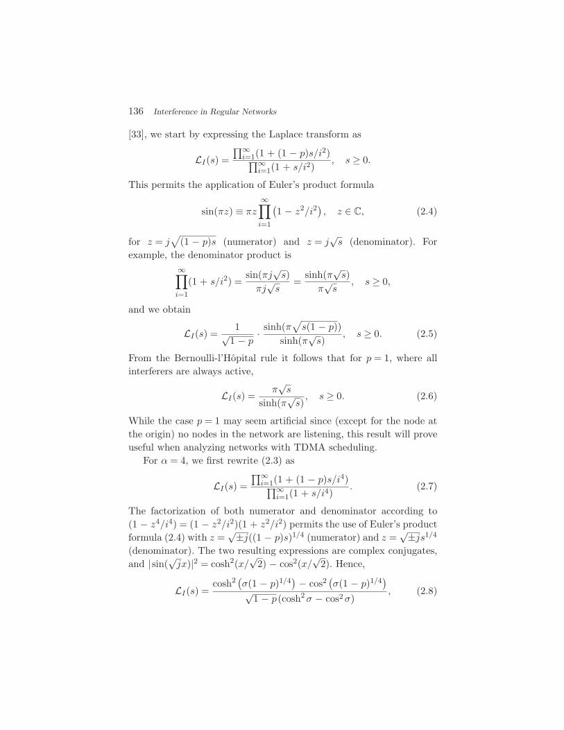
136 Interference in Regular Networks
[33], we start by expressing the Laplace transform as
LI(s) =∏∞i=1(1 + (1 − p)s/i2)∏∞
i=1(1 + s/i2), s ≥ 0.
This permits the application of Euler’s product formula
sin(πz) ≡ πz∞∏i=1
(1 − z2/i2
), z ∈ C, (2.4)
for z = j√
(1 − p)s (numerator) and z = j√s (denominator). For
example, the denominator product is∞∏i=1
(1 + s/i2) =sin(πj
√s)
πj√s
=sinh(π
√s)
π√s
, s ≥ 0,
and we obtain
LI(s) =1√
1 − p ·sinh(π
√s(1 − p))
sinh(π√s)
, s ≥ 0. (2.5)
From the Bernoulli-l’Hopital rule it follows that for p = 1, where allinterferers are always active,
LI(s) =π√s
sinh(π√s), s ≥ 0. (2.6)
While the case p = 1 may seem artificial since (except for the node atthe origin) no nodes in the network are listening, this result will proveuseful when analyzing networks with TDMA scheduling.
For α = 4, we first rewrite (2.3) as
LI(s) =∏∞i=1(1 + (1 − p)s/i4)∏∞
i=1(1 + s/i4). (2.7)
The factorization of both numerator and denominator according to(1 − z4/i4) = (1 − z2/i2)(1 + z2/i2) permits the use of Euler’s productformula (2.4) with z =
√±j((1 − p)s)1/4 (numerator) and z =
ñjs1/4
(denominator). The two resulting expressions are complex conjugates,and |sin(
√jx)|2 = cosh2(x/
√2) − cos2(x/
√2). Hence,
LI(s) =cosh2 (σ(1 − p)1/4
)− cos2
(σ(1 − p)1/4
)√
1 − p(cosh2σ − cos2σ), (2.8)
2.2 One-Dimensional Lattices 137
where σ πs1/4/√
2. For p = 1, this simplifies to
LI(s) =2σ2
cosh2σ − cos2σ=
π2√scosh2
(πs1/4√
2
)− cos2
(πs1/4√
2
) . (2.9)
2.2.2 Probability Densities
Next we would like to find an expression for the probability densityfunction (PDF) of I. Since a direct calculation does not seem possible,we aim at finding a series expression.
For a finite number of nodes n, unit transmit powers, p = 1 (allnodes transmit), and a general path loss exponent α, In is an n-stagehypoexponential random variable with Laplace transform
LIn(s) =n∏i=1
iα
iα + s, (2.10)
whose partial fraction expansion is given by
LIn(s) =n∑i=1
an,iiα
iα + s, where an,i
n∏k=1k =i
kα
kα − iα .
By inverse transformation of each term we obtain the PDF
fIn(x) =n∑i=1
an,iiα exp(−iαx), x ≥ 0. (2.11)
Since the product-form (2.10) has the product∏ni=1 i
α in the numerator(and no term in s), the residue coefficients an,i have the propertiesthat
∑ni=1an,i = 1, n ∈ N, and
∑ni=1an,ii
α = 0 for n > 1. It follows thatfIn(0) = 0 for n > 1. For n = 1, I1 follows an exponential distribution,which implies fI1(0) = 1.
For two special cases, α = 2 and α = 4, we can derive the limitingdistribution limn→∞ fIn(x).
138 Interference in Regular Networks
Special case α = 2. Using Euler’s summation formula again,
1a∞,i
= limx→i
∞∏k=1k =i
(1 − x2/k2)
= limx→i
sin(πx)πx(1 − (x/i)2)
= limx→i
π cos(πx)π(1 − (x/i)2) − πx(2x/i2)
=(−1)i+1
2.
The PDF of the interference as n→∞ is thus
fI(x) =
2∑∞
i=1(−1)i+1i2 exp(−i2x) if x > 0
0 if x = 0.(2.12)
Figure 2.1 shows the densities fIn(x) for n = 2,5,12,∞. The meaninterference in the infinite case is E(I) =
∑∞i=1 i
−2 = ζ(2) = π2/6. Thecorresponding cumulative distribution function (CDF) for finite n is
FIn(x) =n∑i=1
an,i(1 − exp(−i2x)), x ≥ 0, (2.13)
and, for n→∞, since∑n
i=1an,i = 1 for all n ∈ N,
FI(x) =
1 + 2
∑∞i=1(−1)i exp(−i2x) if x > 0
0 if x ≤ 0.(2.14)
Special case α = 4. Proceeding as for α = 2,
1a∞,i
= limx→i
∞∏k=1k =i
(1 − x4/k4)
= limx→i
n∏k=1k =i
(1 − i2/k2)n∏k=1k =i
(1 + i2/k2)
2.2 One-Dimensional Lattices 139
0 1 2 3 40
0.1
0.2
0.3
0.4
0.5
0.6
x
f n(x)
Fig. 2.1 The dashed curves show the probability density fIn (x) from (2.11) for α = 2 andn = 2 (left-most curve), n = 5, and n = 12, and the solid curve shows the limiting densityfI(x) from (2.12).
= limx→i
sin(πx)sinh(πx)(πx)2(1 − (x/i)4)
= limx→i
π cos(πx)sinh(πx) − π sin(πx)cosh(πx)2π2(1 − (x/i)4) − π2x(4x4/i4)
=(−1)i+1 sinh(iπ)
4πi.
Due to the sinh term, the coefficients a∞,i decay very quickly, and itis sufficient to consider only the nearest three or even two interferers.Considering only the nearest interferer yields approximately the righttail of the density, but the probabilities of seeing little interference aredrastically different. This is essentially a diversity effect.
The probability density for the interference as n→∞ is thus
fI(x) =
4π∞∑i=1
(−1)i+1i
sinh(iπ)i4 exp(−i4x) if x > 0
0 if x = 0.
(2.15)
Figure 2.2 shows the densities fIn(x) for n = 1,2,3,∞. The curve forn = 3 is virtually indistinguishable from the limiting case. The meaninterference in the infinite case is E(I) =
∑∞i=1 i
−4 = ζ(4) = π4/90.

140 Interference in Regular Networks
0 0.5 1 1.5 20
0.2
0.4
0.6
0.8
1
x
f n(x)
Fig. 2.2 The dashed curves show the probability density fIn (x) from (2.11) for α = 4 andn = 1,2,3, and the solid curve shows the limiting density fI(x) from (2.15).
2.3 Two-Dimensional Lattices
2.3.1 Square Lattice
Consider a network with nodes arranged in the integer lattice withoutthe origin Z
2 \ o. What is the interference measured at the origin(without fading), or what is the mean interference (with fading)? Thelattice sum
I =∑x∈Z
2
x =o
(‖x‖)
does not have a closed-form expression. However, by grouping the nodesinto rings of increasing distances from the origin, we can give goodbounds. For example, take the four nearest nodes (distance 1), the fournext-nearest (distance
√2), and then (square) rings of 8k nodes for
k = 2,3, . . .. Each node in ring k is at least at distance k and at mostat distance
√2k, which yields the bounds
4(1) + 4(√
2) +∞∑k=2
8k(√
2k) < I < 4(1) + 4(√
2) +∞∑k=2
8k(k).
2.3 Two-Dimensional Lattices 141
For (r) = r−α,
4(1 + 2−α/2) + 8 · 2−α/2(ζ(α − 1) − 1)
< I < 4(1 + 2−α/2) + 8(ζ(α − 1) − 1). (2.16)
For α = 4, this is approximately 5.4 < I < 6.6. The correct value is rightin between, I = 6.037. A better lower bound is obtained if the averagedistance to the nodes in ring k is upper bounded by k(1 +
√2)/2. This
is an upper bound since
k(1 +√
2)2
≥ 12
(√k2 + i2 +
√k2 + (k − i)2
), ∀0 ≤ i ≤ k.
This gives the bound
I ≥ 4(1 + 2−α/2) + 8 ·(
1 +√
22
)−α
(ζ(α − 1) − 1). (2.17)
For α = 4, this is about 5.76. Claiming that the average node distancein ring k is about k
√5/4, obtained from an estimate of k along one
axis and k/2 along the other, gives the very good approximation
I ≈ 4(1 + 2−α/2) + 8 · (5/4)−α/2(ζ(α − 1) − 1). (2.18)
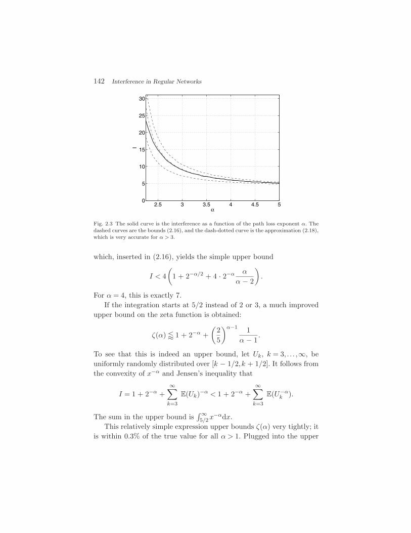
For α = 4, this gives I ≈ 5 + 8(4/5)2(ζ(3) − 1) = 6.034, which is veryaccurate. Figure 2.3 shows the exact value of I as a function of α, plusthe bounds (2.16) and the approximation (2.18).
To obtain closed-form results (without the zeta function) we notethat
∞∑k=3
k−α =∫ ∞
2x−αdx <
∫ ∞
2x−αdx,
whereas∞∑k=3
k−α =∫ ∞
3x−αdx >
∫ ∞
3x−αdx.
x and x denote the smallest integer larger than or equal to x andthe largest integer smaller than or equal to x, respectively. It followsthat
ζ(α) < 1 + 2−α +∫ ∞
2x−αdx = 1 + 2−αα + 1
α − 1, α > 1,
142 Interference in Regular Networks
2.5 3 3.5 4 4.5 50
5
10
15
20
25
30
α
I
Fig. 2.3 The solid curve is the interference as a function of the path loss exponent α. Thedashed curves are the bounds (2.16), and the dash-dotted curve is the approximation (2.18),which is very accurate for α > 3.
which, inserted in (2.16), yields the simple upper bound
I < 4(
1 + 2−α/2 + 4 · 2−α α
α − 2
).
For α = 4, this is exactly 7.If the integration starts at 5/2 instead of 2 or 3, a much improved
upper bound on the zeta function is obtained:
ζ(α) 1 + 2−α +(
25
)α−1 1α − 1
.
To see that this is indeed an upper bound, let Uk, k = 3, . . . ,∞, beuniformly randomly distributed over [k − 1/2,k + 1/2]. It follows fromthe convexity of x−α and Jensen’s inequality that
I = 1 + 2−α +∞∑k=3
E(Uk)−α < 1 + 2−α +∞∑k=3
E(U−αk ).
The sum in the upper bound is∫∞5/2x
−αdx.This relatively simple expression upper bounds ζ(α) very tightly; it
is within 0.3% of the true value for all α > 1. Plugged into the upper
2.3 Two-Dimensional Lattices 143
bound in (2.16), this yields 6.64 for α = 4, so indeed it does not appre-ciably weaken the bound.
In the case of the power law path loss, we may also use results onlattice sums, see, e.g., [55], which typically involve the zeta and otherspecial functions, to express the interference. For the square integerlattice,
I = 4ζ(α/2)β(α/2),
where
β(x) ∞∑i=1
(−1)i+1
(2i − 1)x
is the Dirichlet beta function. β(2) is Catalan’s constant K = 0.916.So, for α = 4, I = 2π2K/3 ≈ 6.03. Whereas for other even-dimensionalsquare lattices, similar expressions are known, there are only approxi-mations available for the three-dimensional case.
2.3.2 Triangular Lattices
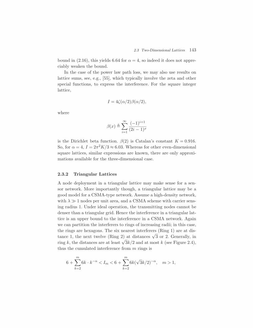
A node deployment in a triangular lattice may make sense for a sen-sor network. More importantly though, a triangular lattice may be agood model for a CSMA-type network. Assume a high-density network,with λ 1 nodes per unit area, and a CSMA scheme with carrier sens-ing radius 1. Under ideal operation, the transmitting nodes cannot bedenser than a triangular grid. Hence the interference in a triangular lat-tice is an upper bound to the interference in a CSMA network. Againwe can partition the interferers to rings of increasing radii; in this case,the rings are hexagons. The six nearest interferers (Ring 1) are at dis-tance 1, the next twelve (Ring 2) at distances
√3 or 2. Generally, in
ring k, the distances are at least√
3k/2 and at most k (see Figure 2.4),thus the cumulated interference from m rings is
6 +m∑k=2
6k · k−α < Im < 6 +m∑k=2
6k(√
3k/2)−α, m > 1,

144 Interference in Regular Networks
Fig. 2.4 A triangular lattice with three hexagonal rings of nodes. Assuming unit nearest-neighbor distances, the two circles indicate that the nodes in the second ring are at distanceat least
√3 and at most 2. Generally, the distance to the nodes in the k-th ring is lower
bounded by√
3k/2 and upper bounded by k. Ring k contains 6k nodes.
and, for m→∞,
6ζ(α − 1) < I < 6(
1 +(
2√3
)α(ζ(α − 1) − 1)
). (2.19)
2.4 Outage
As discussed in Section 1.2.2 (p. 133), the outage in Rayleigh fad-ing follows directly from the Laplace transform. So, in all the trans-forms derived, we obtain the (noise-free) success probability simplyby replacing s by the SINR threshold θ. The noise factor is pWs =exp(−θW/(P(r))), where P is the transmit power of the desired trans-mitter and r is the distance of the link. So the interference factor pIs ismuch more critical, and for notational simplicity, we henceforth dropthe superscript I in pIs.
As a sanity check, let us first consider the general case determin-istic case (2.3) and let θ→∞. We obtain limθ→∞ ps(θ) = (1 − p)n, asexpected, since a transmission can only succeed if there is no activeinterferer.
2.4.1 ALOHA in One-Dimensional Line Networks
The success probabilities for ALOHA for one-sided line networks followimmediately from the corresponding Laplace transforms. From (2.5) it

2.4 Outage 145
follows that for α = 2,
ps(θ) =1√
1 − p ·sinh(π
√θ(1 − p))
sinh(π√θ)
, (2.20)
and for α = 4, it follows from (2.8),
ps(θ) =cosh2 (σ(1 − p)1/4
)− cos2
(σ(1 − p)1/4
)√
1 − p(cosh2σ − cos2σ), (2.21)
where σ πθ1/4/√
2.
2.4.2 TDMA in One-Dimensional Line Networks
Here we assume that interferers are scheduled in an m-phase TDMAfashion. In a one-sided line network, this means that nodes 1,1 + m,1 +2m,. . . transmit in slot 1, nodes 2,2 + m,2 + 2m,. . . transmit in slot2, and so on, until slot m in which the nodes in mN transmit. Afterthat, the first set of nodes transmits again. In terms of interference,this means that the network is stretched by a factor m, i.e., all thedistances are increased by m, and the interference from each node isnow
∑∞i=1 (im) instead of just summing over (i). For the power law
path loss model, this means all powers are reduced by mα. But this isequivalent to reducing the SIR threshold θ by the same factor! So wecan simply take the Laplace transforms for p = 1, (2.6) and (2.9), andreplace s by θm−α instead of by θ to obtain the success probabilitiesfor TDMA.
For α = 2, we obtain from (2.6),
ps(θ) =σ
sinhσ, where σ π
√θ
m, (2.22)
and for α = 4, from (2.9),
ps(θ) =2σ2
cosh2σ − cos2σ, where σ πθ1/4
√2m
. (2.23)
Since θ enters these expressions only through θ1/α and m-phase TDMAreduces the threshold by mα, the exponents for m cancel, and theparameter σ is simply inversely proportional to m.
146 Interference in Regular Networks
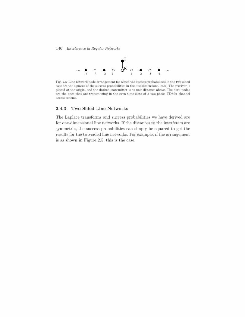
...
T
R4 3 2 1 1 2 3 4
...
Fig. 2.5 Line network node arrangement for which the success probabilities in the two-sidedcase are the squares of the success probabilities in the one-dimensional case. The receiver isplaced at the origin, and the desired transmitter is at unit distance above. The dark nodesare the ones that are transmitting in the even time slots of a two-phase TDMA channelaccess scheme.
2.4.3 Two-Sided Line Networks
The Laplace transforms and success probabilities we have derived arefor one-dimensional line networks. If the distances to the interferers aresymmetric, the success probabilities can simply be squared to get theresults for the two-sided line networks. For example, if the arrangementis as shown in Figure 2.5, this is the case.
3Interference in Poisson Networks
In this section we focus on networks whose nodes are distributed as ahomogeneous Poisson point process (PPP) (see Section A.1.2). Amongall stochastic node distribution models, the PPP and the closely relatedbinomial point process (see Section A.1.1), where a fixed number ofnodes is uniformly randomly placed in a certain area, are by far themost popular; they are used in certainly more than 95%, perhaps 99% ofthe analytical work on wireless network characterization. The completespatial randomness or independence property makes the PPP easy toanalyze. From the practical side, the PPP model is often justified byclaiming that it is suitable when large numbers of nodes are droppedfrom aircraft (in sensor networks), or when nodes move around inde-pendently and uniformly in a certain area.
While interference characterization in large wireless systems is arelatively new topic, a similar type of noise, the so-called shot noise,has been the subject of investigation for more than a century already.We start our discussion by drawing parallels between shot noise andinterference.
147
148 Interference in Poisson Networks
3.1 Shot Noise
If the nodes in the network are distributed according to a stochasticpoint process, the interference function stated in (1.1), can be viewedas a random field or, more specifically, as a shot noise process. In onedimension, a basic shot noise process is described as
I(t) =∞∑i=1
g(t − xi) =∑x∈Φ
g(t − x), (3.1)
where Φ = xi∞i=1 is a stationary Poisson process on R and g(x) is theimpulse response. Traditionally, shot noise is measured in time, i.e., thepoints in the PPP are time instants. To model interference in a (one-dimensional) wireless network, we replace the time axis by the spatialaxis and the impulse response g(x) with the path loss function (‖x‖).This spatial impulse response is two-sided and even, since the wirelesssignals are assumed to spread equally in both directions. This way, (3.1)becomes the expression for the interference in a one-dimensional net-work whose (transmitting) nodes are distributed as a Poisson process,with unit transmit powers and no fading.
A generalized shot noise process permits the incorporation of astochastic impulse response and multi-dimensional point processes:
I(y) =∞∑
x∈Φ
Kxg(y − x), (3.2)
where the coefficients Kx are iid random variables that can be used tomodel fading. Putting Kg(x) = h(‖x‖) shows that (1.1) is a specialcase of (3.2).
Shot noise processes have been studied at least dating back toCampbell in 1909 [6, 7], who characterized their mean and variance,more fully by Schottky in 1918 [41], while Rice [39] and later Gilbertand Pollak [15] performed extensive investigations on their distribu-tion. Since the path loss law (·) is typically a power law, power lawshot noise is most relevant in the context of wireless networks. It wasconsidered by Lowen and Teich in 1990 [32]. In particular, they showedthat it does not converge to a normal distribution as the intensity of thepoint process increases, in contrast to exponentially decaying impulse
3.2 Interference Distribution 149
responses. Heinrich and Schmidt studied normal convergence of shotnoise processes in detail in [25].
3.2 Interference Distribution
In this section we would like to characterize the total interference powermeasured at the origin, given by
I = I(o) ∑x∈Φ
hx(‖x‖), (3.3)
where Φ is a point process of interferers on Rd. In this case of a uniform
(or homogeneous) PPP, it does not matter where the interference ismeasured; due to Slivnyak’s theorem (Theorem A.5) it could even bemeasured at a point of the process as long as its contribution to I fromthat point is not considered. In all other cases, however, it does, sincethe interference seen by a typical point of the point process differs fromthe interference seen at an arbitrary point of the plane (see Section A.2on Palm distributions in the appendix).
For channel access, ALOHA is a natural match for the PPP, sinceALOHA maintains the distributional properties of the PPP: If all nodesform a PPP of intensity λ and transmit independently with probabil-ity p, the set of transmitters forms a PPP of intensity pλ. This followsfrom the (independent) thinning property of the PPP, see Section A.1.2in the appendix. This implies that if I(λ) is the interference in a PPPof intensity λ where all nodes transmit, I(pλ) is the interference in thesame network when ALOHA with probability p is used. Further, due tothe superposition property of the PPP, the interference is proportionalto λ, or pλ.
3.2.1 Mean Interference
We start the discussion with a brief derivation of the mean interference.From Campbell’s theorem (Theorem A.2), we have
E(I) =∑x∈Φ
hx(‖x‖) = λE(h)∫
Rd
(‖x‖)dx
= λcdd
∫ ∞
0(r)rd−1dr,

150 Interference in Poisson Networks
where cd = |b(o,1)| is the volume of the d-dimensional unit ball. Thefading distribution does not matter, as long as E(h) = 1. For (r) = r−α,
E(I) = λcdd
∫ ∞
0rd−α−1 =
λcdd
d − αrd−α
∣∣∣∞0. (3.4)
This diverges for α < d due to the upper integration bound, i.e., thecumulated interference from the large number of distance nodes. Forα > d, it diverges due to the lower bound, which is a consequence of thepath loss law and the property of the PPP that nodes can be arbitrarilyclose. For α = d, both the lower and upper bounds cause problems.
For finite networks, α < d guarantees a finite mean, but in the infi-nite case it results in infinite interference a.s. On the other hand, forα > d, the interference is finite a.s. even for infinite networks since theLaplace transform is non-degenerate, as we will show.
In practice, the path loss is bounded, which can be modeled by, e.g.,(r) = min(1, r−α). In this case, the mean exists for α > d. For finitetwo-dimensional networks of radius ρ > 1,
E(Iρ) = λ
(π +
2πα − 2
(1 − ρ2−α)) .
This simple calculation gives some guideline on how large to choosethe network area in a simulation, where the behavior of an infinitenetwork is to be explored. If the mean interference in the simulationarea (outside radius 1) should match the theoretical mean in an infinitenetwork up to a factor 1 − ε, we have
1 − ρ2−α > 1 − ε =⇒ ρ > ε−1/(α−2). (3.5)
For example, if ε = 10−3 and α = 2.5, the radius has to be at least 106.For values of α smaller than 2.1, the network can hardly be simulatedexactly. On the other hand, for α = 4, a radius of only 32 is sufficientto get within 0.1%. More details on the complexity of simulating PPPscan be found in [50]. The paper also describes how to add a correctionterm to the interference if the simulation area cannot be chosen largeenough to yield the desired accuracy.
3.2 Interference Distribution 151
3.2.2 Interference Distribution Without Fading
In this subsection we focus on the case of two-dimensional networksand assume there is no fading, i.e., hx ≡ 1 in (3.3), and our goal is tofind the characteristic function of the interference and from there, ifpossible, the distribution.
We follow a basic yet powerful technique as it was used, for example,in [43]. It consists of two steps:
1. Consider first a finite network, say on a disk of radius a cen-tered at the origin, and condition on having a fixed numberof nodes in this finite area. The nodes’ locations are then iid.
2. Then de-condition on the (Poisson) number of nodes and letthe disk radius go to infinity.
Step 1. Consider the interference from the nodes located within distancea of the origin:
Ia =∑
x∈Φ∩b(o,a)(‖x‖). (3.6)
For the path loss law (x), it is assumed that it is strictly monotonicallydecreasing (invertible), and that limx→∞ (x) = 0. In the limit a→∞,Ia = I. Let FIa be the characteristic function (Fourier transform) of Ia,i.e.,
FIa(ω) E(ejωIa). (3.7)
Conditioning on having k nodes in the disk of radius a,
FIa(ω) = E(E(ejωIa | Φ(b(o,a)) = k)
). (3.8)
Given that there are k points in b(o,a), these points are iid uniformlydistributed on the disk with radial density
fR(r) =
2ra2 if 0 ≤ r ≤ a0 otherwise,
(3.9)
and the characteristic function is the product of the k individual char-acteristic functions:
E(ejωIa | Φ(b(o,a)) = k) =(∫ a
0
2ra2 exp(jω(r))dr
)k. (3.10)
152 Interference in Poisson Networks
Step 2. The probability of finding k nodes in b(o,a) is given by thePoisson distribution, hence:
FIa(ω) =∞∑k=0
exp(−λπa2)(λπa2)k
k!E(ejωIa | Φ(b(o,a)) = k). (3.11)
Inserting (3.10), summing over k, and interpreting the sum as the Tay-lor expansion of the exponential function, we obtain
FIa(ω) = exp(λπa2
(−1 +
∫ a
0
2ra2 exp(jω(r))dr
)). (3.12)
Integration by parts, substituting r→ −1(x), where −1 is the inverseof , and letting a→∞ yields
lima→∞
a2(−1 +
∫ a
0
2ra2 exp(jω(r))dr
)=∫ ∞
0(−1(x))2jωejωxdx,
so that
FI(ω) = exp(jλπω
∫ ∞
0(−1(x))2ejωxdx
). (3.13)
To get more concrete results, we need to specify the path loss law. Forthe standard power law (r) = r−α, we obtain
FI(ω) = exp(jλπω
∫ ∞
0x−2/αejωxdx
). (3.14)
For α ≤ 2, the integral diverges, indicating that the interference is infi-nite almost surely. For α > 2,
FI(ω) = exp(−λπΓ(1 − 2/α)ω2/αe−jπ/α
), ω ≥ 0. (3.15)
The values for negative ω are determined by the symmetry conditionF∗I (−ω) = FI(ω). For α = 4,
FI(ω) = exp(−λπ3/2 exp(−jπ/4)
√ω). (3.16)
This case is of particular interest, since it is the only one where aclosed-form expression for the density exists:
fI(x) =πλ
2x3/2 exp(−π
3λ2
4x
). (3.17)
3.2 Interference Distribution 153
This is the so-called Levy distribution, which can also be viewed asan inverse gamma distribution, or as the inverse Gaussian distributionwith infinite mean. For other values of α, the densities may be expressedin an infinite series [43, Equation (22)].
The characteristic function (3.15) indicates that the interference dis-tribution is a stable distribution with characteristic exponent 2/α < 1,drift 0, skew parameter β = 1, and dispersion λπΓ(1 − 2/α)cos(π/α).See Section A.3 for an introduction to stable random variables, in par-ticular (A.14); many more details are given in [40]. The correspondingLaplace transform is (see (A.15))
LI(s) = exp(−λπΓ(1 − 2/α)s2/α). (3.18)
Stable distributions with characteristic exponents less than one donot have any finite moments. In particular, the mean interferencediverges, which is due to the singularity of the path loss law atthe origin. This also follows immediately from the fact that E(I) =− d
ds log(LI(s))|s=0 = lims→∞ cs2/α−1 =∞. In fact, even when only thenearest interferer, at distance R1, is considered, the mean E(I) doesnot exist: For α ≥ 2,
E(I1) = E(R−α1 ) =
∫ ∞
02πλx1−α exp(−λx2)dx =∞.
The method of conditioning on a fixed number of nodes, using theiid property of the node locations, and de-conditioning with respect tothe Poisson distribution is applicable to many other problems.
3.2.3 Interference Distribution with Fading
Here we derive the interference as given in (3.3) for Rayleigh fading.We pursue two separate approaches.
De-conditioning on deterministic network. A first approach,which has been used in [33], is to use the Laplace transform for gen-eral deterministic networks (2.3) and de-condition on the distances ofthe nodes from the origin. In the one-dimensional case, the n smallest

154 Interference in Poisson Networks
distances from the origin 0 ≤ R1 ≤ R2 ≤ . . . ≤ Rn are governed by thejoint distribution
f(R1,...,Rn)(r1, . . . , rn) = (2λ)n exp(−2λrn)1K(r1, . . . , rn),
where K = (r1, . . . , rn) | 0 ≤ r1 ≤ r2 ≤ . . . ≤ rn is the order cone orhyperoctant in R
n, and 1K is the indicator function (see, e.g., [20,Corollary 2]). The factor two stems from the fact that the networkextends over the whole real line R, so the point process of distancesfrom the origin |xi| has density two.
For α = 2, (2.3) is now the conditional Laplace transform
LcIn(s) = E(exp(−sIn) | R1 = r1, . . . ,Rn = rn)
=n∏i=1
r2ir2i + s
, s ≥ 0.
The superscript c indicates conditioning. Integrating with respect tothe joint density yields the de-conditioned Laplace transform
LIn(s) =∫Kλn exp(−2λrn)
n∏i=1
r2ir2i + s
dr1 · · ·drn
=(2λ)n+1
n!
∫ ∞
0exp(−2λr)
(r −√sarctan(r/
√s))ndr, (3.19)
where the second line is obtained using induction and partial integra-tion [33]. For all n ∈ N, LIn(0) = 1, and it can be shown that the limitlimn→∞LIn(s) exists for all s. So, by continuity, the distribution ofthe interference I∞ is not defective. Similarly, it can be shown that inthe two-dimensional case with α = 2, the interference distribution isdefective, i.e., P(I∞ =∞) = 1.
For α = 4 in the two-dimensional case, the squared distances fromthe origin form again a homogeneous PPP, this time of intensity λπ. So,merely by changing 2λ to πλ in (3.19), we obtain the Laplace transformof the interference caused by the first n interferers in two-dimensionalnetworks for α = 4. Figure 3.1 shows the Laplace transforms for theone- and two-dimensional cases. It can be seen that the transformsconverge quickly.

3.2 Interference Distribution 155
0 2 4 6 8 100.2
0.3
0.4
0.5
0.6
0.7
0.8
0.9
1one–dimensional network, α=2
s
Lapl
ace
tran
sfor
m L
(s)
n=1n=2n=5n=100
0 2 4 6 8 100.2
0.3
0.4
0.5
0.6
0.7
0.8
0.9
1two–dimensional network, α=4
s
Lapl
ace
tran
sfor
m L
(s)
n=1n=2n=5n=100
Fig. 3.1 Laplace transform LIn (s) for the one-dimensional (left) and two-dimensional(right) cases. n = 1,2,5,100. The curve for n = 1 is the top curve.
While these are useful results, they are not closed-form; in par-ticular, it does not seem possible to find an explicit expression for thelimiting Laplace transform for n→∞ from (3.19). Thus we will pursuea different approach to find the Laplace transform of the interferencein an infinite network.
Using the probability generating functional. As mentioned inSection 3.1, researchers have found an analogy to shot noise processesto analyze the distributional properties of I(x) [26, 32, 39].
Here we are using this insight to derive the Laplace transform of theinterference. First we map the d-dimensional PPP onto R
+ by lettingΦ ri = ‖xi‖ be the distances of the points of a d-dimensional uni-form PPP of intensity λ. Per the mapping theorem (Theorem A.1,see also [30]), Φ is an inhomogeneous PPP with intensity functionλ′(r) = λcddr
d−1, where cd = |b(o,1)| is the volume of the d-dimensionalunit ball. Considering the interference as a shot noise process (3.1), wecan identify the path loss law (r) = hrr
−α for iid h with the impulseresponse of the shot noise process. We would like to calculate theLaplace transform
LI(s) E[e−sI ] = E
[exp
(−s
∑r∈Φ
hrr−α)]
156 Interference in Poisson Networks
of the interference. The expectation is to be taken over both the pointprocess and the fading. Due to the independence of the fading,
LI(s) = EΦ
[∏r∈Φ
Eh
[exp
(−shrr−α
)]].
This is a probability generating functional (see Definition A.5) withv(r) = Eexp(−shrr−α), so we have from (A.3)
LI(s) = exp− Eh
(∫ ∞
0(1 − exp(−shr−α))λ′(r)dr︸ ︷︷ ︸
A
),
where we flipped the order of integration and expectation. First wecalculate the integral:
A = λcd
∫ ∞
0
(1 − exp(−shr−α)
)drd−1dr
= λcd
∫ ∞
0
(1 − exp(−shr−1/δ)
)dr (subst. r← rd)
= λcd
∫ ∞
0
(1 − exp(−sh/x)
)δxδ−1dx (subst. x← r1/δ),
where δ d/α. To calculate this integral, we note that it is the expectedvalue
E[((X/sh)−1)δ]
of an exponential random variable X with mean 1. Since E(Xp) =Γ(1 + p) by the definition of the gamma function,
Γ(p) ∫ ∞
0tp−1e−tdt,
it follows that
E[((X/sh)−1)δ] = (sh)δΓ(1 − δ).
So, with A = λcd(hs)δΓ(1 − δ), we obtain
LI(s) = exp(− λcdE[hδ]Γ(1 − δ)sδ
). (3.20)
3.2 Interference Distribution 157
The only difference to (3.18) is the additional term E(hδ), whichaccounts for the fading. For non-unit transmit powers Pt, s is simplyreplaced by Pts, i.e., the transmit powers enters the Laplace transformthrough an additional factor P δt in the exponential. Note that (3.20) isonly valid for δ < 1. So:
• For α ≤ d, we have I =∞ a.s. This is a consequence of thecumulated interference from the many far transmitters whosesignal powers do not decay fast enough to keep the interfer-ence power finite. For a finite network, the interference wouldbe finite.
• For α > d we have I <∞ a.s. but E(I) =∞ due to the sin-gularity of the path loss law at the origin. Even if we consideronly the nearest interferer, E(I) is infinite. If a bounded pathloss law is used, all moments exist.
In the case of Rayleigh fading, E(hδ) = Γ(1 + δ), using the propertiesof the gamma function, we obtain the closed-form result
LI(s) = exp(− λcdsδ
πδ
sin(πδ)
). (3.21)
As in the non-fading case, the interference has a stable distributionwith characteristic exponent δ, drift 0, and skew parameter β = 1; thedispersion here is λcdE(hδ)Γ(1 − δ)cos(δπ/2), see Section A.3.
As shown in (3.17), for δ = 1/2, the PDF and CDF exist. WithΓ(3/2) =
√π/2, the Levy PDF is in the two-dimensional case (α = 4)
fI(x) =λ
4
(πx
)3/2exp
(−π
4λ2
16x
), (3.22)
and the CDF is
FI(x) = 1 − erf(π2λ
4√x
), (3.23)
where erf(x) = 2∫ x0 exp(−t2)dt/
√π is the standard error function.
158 Interference in Poisson Networks
For general δ, the probability density of the interference can beexpressed as [32]
fI(x) =1πx
∞∑i=1
(−1)i+1Γ(1 + iδ)sin(πiδ)i!
·(λcdΓ(1 − δ)E(hδ)
xδ
)i.
(3.24)From this series it is apparent that as x→∞, the term for i = 1becomes dominant, and
fI(x) ∼1
πxδ+1λcdΓ(1 + δ)Γ(1 − δ)sin(πδ)︸ ︷︷ ︸πδ
E(hδ)
∼ λcdδE(hδ)x−(1+δ), x→∞. (3.25)
In the non-fading case, we may use the distribution of the distancesto the n-th nearest neighbor to generalize this result to the behavior ofthe tail probability for the n-th interferer. The CCDF of the distanceto the n-th nearest neighbor Rn is [19]
P(Rn > r) =n−1∑k=0
(λcdrd)k
k!exp(−λcdrd) =
Γ(n,λcdrd)Γ(n)
,
where Γ(·, ·) is the upper incomplete gamma function. So, with In =R−αn ,
P(In < x) =n−1∑k=0
(λcdx−δ)k
k!exp(−λcdx−δ) =
Γ(n,λcdx−δ)Γ(n)
. (3.26)
For the tail probability we need the CCDF, obtained by summingfrom n to ∞ instead of 0 to n − 1. For x→∞, the dominant term willbe the one for k = n. Since exp(−x−δ) ∼ 1 − x−δ,
P(In > x) ∼ (1 − λcdx−δ)(λcdx−δ)n
n!
∼ 1n!
(λcd)nx−nδ, x→∞. (3.27)
Plugging in n = 1 and taking the derivative, it is confirmed that this isconsistent with (3.25).
These results on the tail probabilities imply that E(Ipn) exists forp < nδ. For example, if interference-canceling techniques are used and
3.2 Interference Distribution 159
the interference from the k nearest interferers can be canceled, we needk > α in two-dimensional networks to have a finite second moment.
With fading, we can infer from (3.24) that a factor (E(hδ))n has tobe added.
The fact that the fading distribution only enters the Laplace trans-form (3.20) through its δ-th moment may appear surprising at first. Itis, however, an instance of a result by Gilbert and Pollak [15] (see also[32]) who have shown that in the one-dimensional case, an ensembleof stochastic response functions, in our case hx−α, has an equivalentdeterministic impulse response function eq(x) = cx−α satisfying
Eh|x : hx−α > y| = |x : cx−α > y| ∀y.
To find c, we note that the LHS is E(h1/α)x−1/α, and the RHS isc1/αx−1/α. So c = (E(h1/α))α. So, replacing (r) = r−α by eq(r) =(E(h1/α))αr−α gives the correct first-order statistics for the interferencewith fading process h in the one-dimensional case. In d dimensions, theLHS is cdE(hδ)x−δ, and the RHS is cdcδx−δ, and the equivalent deter-ministic path loss law is
eq(r) = (E(hδ))1/δr−α.
As an example, plugging in this deterministic path loss law in (3.14)yields the correct expression for the Laplace transform for the fad-ing case (3.20), since x−δ in (3.14) is replaced by (x/c)−δ, which pro-duces the factor E(hδ) as desired. The equivalence only holds up to themean, but since these distributions do not have any finite moments, theLaplace transforms for the cases with stochastic fading and with theequivalent deterministic path loss law are identical. As we can see fromthe series expression of the probability density (3.24), the completedensity cannot be derived using the equivalent path loss law.
In [26] the amplitude distribution of the interference was stud-ied; they show that if each interfering signal is spherically symmetric,the interference amplitude has a symmetric Levy-stable distribution(skew 0) with characteristic exponent 4/α. This is consistent with ourresult for the interference power, since the amplitude decays with dis-tance to the power α/2. They also analyzed the convergence properties
160 Interference in Poisson Networks
to stable distribution as the number of nodes increases, and they con-sidered lognormal fading (shadowing).
3.3 SIR Distribution and Outage
As mentioned in the introduction, the Laplace transform is exactlythe distribution of the SIR if the power from the desired transmittersS is exponentially distributed (Rayleigh fading). So while closed-formexpressions for the interference itself do not exist, they are available incertain cases for the SIR.
For a transmitter–receiver distance r, the received signal power Sis exponential with mean r−α. The success probability ps(θ) = P(S >Iθ) = Eexp(−Iθrα) is the Laplace transform of the interference evalu-ated at s = θrα. So, in a d-dimensional interference-limited networkswhose nodes are distributed as a uniform PPP of intensity λ withALOHA channel access with probability p, the outage probability forRayleigh fading desired signal strength S follows from (3.20), replacings by θrα:
ps(θ) = exp(− pλcdrdE(hδ)Γ(1 − δ)θδ
). (3.28)
Here we have used the fact that ALOHA channel access performs inde-pendent thinning of the PPP, which results in a PPP of lower intensity.While S needs to be Rayleigh, the interferers’ channels may be subjectto a different type of fading (or no fading), all that matters is E(hδ).For Rayleigh fading interferers, we obtain from (3.21)
ps(θ) = exp(−pλcdrd
πδ
sin(πδ)θδ). (3.29)
This result has been derived in [3, 54].Since the nearest-neighbor distance scales as λ−1/d, this shows that
nearest-neighbor communication is always possible with constant suc-cess probability, irrespective of the network density.
If the received signal strength from the desired transmitter isnot Rayleigh fading, there are no known closed-form expressions forthe outage. If the fading random variables have a square integrabledensity, an integral expression for the success probability is given

3.4 Extremal Behavior 161
in [4, Proposition 2.2]. Bounds on the outage probability have beenderived in [49, 51] in the context of the so-called transmission capac-ity, defined to be the maximum transmitter density given an outageconstraint for transmissions to a receiver at fixed distance.
3.4 Extremal Behavior
When analyzing the outage probabilities of nearest-neighbor transmis-sion or the benefits of interference cancellation, it is necessary to relatethe power from the strongest interferer to the total interference. Thisstrongest “interferer” may be the desired transmitter or the one to becanceled. Here we derive the extreme value statistics for the maximuminterference in two-dimensional networks. As in Section 3.2.2, we startby putting k nodes uniformly iid on a disk of radius a. For the powerpath loss law, without fading, the power at the origin from each node,R−α, is distributed as
P(R−α < x) = 1 − 1a2x
−2/α, x ≥ a−α.
Let δ 2/α. Let Mk be the maximum of the k interference powers andFMk
(x) its CDF:
FMk(x) =
(1 − 1
a2x−δ)k
, x ≥ a−α.
Since the CCDF decays like x−δ, the asymptotic extremal distribu-tion FM∞ is a Frechet distribution, which has the shape exp(−x−δ),up to a possible shift and dilatation (see, e.g., [18, Theorem 6.2]). Thismeans that there are sequences of shift parameters ak and dilatationparameters bk, such that
limk→∞
FMk(ak + bkx) = exp(−x−δ).
The standard Frechet distribution on the right side is the limitlimk→∞(1 − x−δ/k)k. So ak and bk are given by the identity
FMk(ak + bkx) ≡
(1 − x−δ
k
)k,
162 Interference in Poisson Networks
from which we find ak ≡ 0, bk = (k/a2)1/δ. Hence
FMk(x) ∼ exp(−(k/a2)x−δ) as k→∞. (3.30)
If we let k and a2 go to infinity such that the density λ = k/(πa2) staysconstant, we have
FM∞(x) = exp(−λπx−δ). (3.31)
In this limiting case, the nodes form a PPP on R2, so we should be
able to get the same result by simply calculating the interference R−α1
from the nearest interferer, assumed at distance R1. Indeed, P(R1 <
r) = 1 − exp(−λπr2), from which (3.31) follows immediately.Rewriting the CDF in (3.30) in terms of the rescaled variables
xk−1/δ such that the right side becomes independent of k shows thatMk = Θ(k1/δ). Since δ < 1, k1/δ k for large k, so the sum is not pro-portional to k, which is consistent with the fact that the mean diverges.We have found in Section 3.2 that the distribution of the sum of allinterferers is a Levy-stable distribution with the same power-law tailas the Frechet distribution, which shows that the maximum and thesum are of the same order. This implies, in turn, that if the powerfrom the nearest transmitter is the desired signal, the SIR convergesto a non-zero constant as k→∞. This fact has been exploited in, forexample, in [16] to derive the capacity scaling law for ad hoc networkswith mobile nodes. It hinges, however, critically on the homogeneity ofthe path loss law.
The situation is the same in the presence of fading — as long as theexpectation of the fading random variable is finite, which is generallythe case. Then the heavy tail of the interference distribution can onlybe due to the singularity of the path loss law.
3.5 Power Control
We introduce the notion of perceived transmit power P , which is thetransmit power multiplied by the fading coefficient. Previously, we didnot consider power control but fading, so we had P = h. With neitherfading nor power control, P ≡ 1. With power control and no fading,P is just the transmit power Pt, and with power control and fading,

3.5 Power Control 163
P = hPt. We assume that the power control schemes will result in theperceived transmit powers Pi to be iid across the transmitters, whichallows us to use the result (3.20) from the previous section since forthe interference it does not matter if the randomness is due to fadingor power control, or the combination of both. The main change is toreplace E(hδ) by E(P δ); hence our task in this section is mainly thedetermination of this δ-th moment.
We focus on pairwise power control between a transmitter and itsreceiver; in particular, we consider the case where each node trans-mits to its nearest neighbor, assumed at distance R1. As it would notmake sense to have all nodes in the network transmit, we introducean ALOHA parameter p to obtain a thinned PPP of intensity λp oftransmitters. This changes (3.20) slightly to
LI(s) = exp(− pλcdE(P δ)Γ(1 − δ)sδ
).
3.5.1 Channel Inversion Without Fading
In this case, nodes compensate for the large-scale path loss by channelinversion. The transmit power Pt = P = Rα1 is Weibull distributed
P(P ≤ x) = 1 − exp(− λcdxδ
)with the moments
E(Pm) =Γ(1 + m/δ)
(λcd)m/δ.
One might argue that instead of λ, λ(1 − p) should be used as therelevant density for the nearest-neighbor distance since this is the den-sity of the non-transmitting nodes. This would require a simple changein the network density. However, ALOHA is an uncoordinated MACscheme, so it is not possible for a transmitter to know when its intendedreceiver will be available to actually receive. Since E(P δ) = 1/(λcd) weobtain from (3.20)
LI(s) = exp(− pΓ(1 − δ)sδ
), (3.32)
which is independent of the network density! So, no matter how densewe make the network, if the transmitters talk to their nearest neighbors
164 Interference in Poisson Networks
and compensate for the path loss so that their signal arrives with unitpower, the interference distribution does not change. This is of coursenot a coincidence: If nodes are ordered according to their distancesRi from a given point, Rdi forms a homogeneous PPP of intensityλcd [20, Corollary 2]. So the mean distance to the first node R1 is1/(λcd)1/d. The transmit power is proportional to Rα1 , so P δ = Rd1,which is proportional to 1/(λcd).
Compared to the case without power control, where we assumed unittransmit power, the mean power here is E(P ) = Γ(1 + 1/δ)/(λcd)1/δ.If we compensate for the change in mean transmit power, the powerdistribution is
P(P ≤ x) = 1 − exp(− (Γ(1 + 1/δ)x)δ
),
and the Laplace transform takes the form
LI(s) = exp(− pλcdΓ(1 + 1/δ)−δΓ(1 − δ)sδ
). (3.33)
Comparing the resulting interference with the interference in Rayleighfading (without power control), we note that the coefficients Γ(1 + δ) >Γ(1 + 1/δ)−δ for δ < 1 and that the ratio diverges as δ→ 0 sincelimδ→0 Γ(1 + 1/δ)−δ = 0. This indicates that power control causesless interference than Rayleigh fading would, and that the differenceincreases with increasing path loss exponent α (for a fixed number ofdimensions d).
While the power levels are spatially iid, it cannot be assumed thatthey are also temporally iid, since the distance to a node’s nearestneighbor is unlikely to change from time slot to time slot. The temporalcorrelation structure depends on the level of mobility and the length ofa communication session between two nodes.
3.5.2 Power Control and Fading
Compensation for large-scale path loss. If the channel is Rayleigh fadingbut the transmitters only compensate for the large-scale path loss to thenearest receiver, each interferer’s power is the product of the Weibullrandom variable Rα1 and an exponential random variable h, P = Rα1h.Generally, the product of two independent random variables X and Y
3.5 Power Control 165
with distributions FX(x) and FY (x), respectively, is distributed as
FXY (z) = EY (FX(z/Y )) = EX(FY (z/X)).
In this case, the product distribution is
FP (x) =∫ ∞
0(1 − exp(x/r))λcdδrδ−1 exp(−λcdrδ)dr. (3.34)
This integral can be expressed using the infinite series [35]
FP (x) =(λcd)1/δx∞∑k=0
Γ(1 − 1
δ (k + 1))
(k + 1)!(−(λcd)1/δx)k
+ λcdxδ
∞∑k=0
Γ(1 − δ(k + 1))(k + 1)!
(−λcdxδ)k, (3.35)
which exhibits a striking symmetry between the two parts in thisexpression. This representation is only valid if 1/δ /∈ N since the gammafunction diverges for negative integers.
The moment E(P δ) is easy to find:
E(P δ) = E((Rα1 )δhδ) = E(Rd1)E(hδ) =1λcd
Γ(1 + δ). (3.36)
With this, we obtain
LI(s) = exp(− pΓ(1 + δ)Γ(1 − δ)sδ
), (3.37)
and, for the case where the transmit powers are normalized to 1,
LI(s) = exp(−pλcd
Γ(1 + δ)Γ(1 + 1/δ)δ
Γ(1 − δ)sδ). (3.38)
Compensation for path loss and fading. If the transmitters have thecomplete channel information, including the fading realization, theycan compensate for the complete path loss. The iid process governingthe interference power is Rα1h2/h1, where h1 is the fading coefficient ofthe channel to the transmitter’s destination and h2 is the coefficient ofthe channel to the point where interference is measured, see Figure 3.2.Let H h2/h1. In Rayleigh fading,
FH(x) =x
x + 1.

166 Interference in Poisson Networks
R1
α
h1 T R
h2
h1Pt=
Fig. 3.2 Illustration for the case where power control is used to compensate for large-scalepath loss and fading. Interference is measured at the location of the star. The transmitter Ttransmits at power Pt = Rα
1 /h1 to compensate for its channel to its receiver R. The channelfrom T to the location of the star is subject to fading with coefficient h2, so the perceivedpower is Rα
1 h2/h1.
With P = Rαh2/h1,
FP (x) =∫ ∞
0
1 − exp(−λcd(x/y)δ)(y + 1)2
dy. (3.39)
The δ-moment is of H is
E(Hδ) = E(hδ2) E(h−δ1 ) = Γ(1 + δ)Γ(1 − δ),
from which
E(P δ) =Γ(1 + δ)Γ(1 − δ)
λcd,
and
LI(s) = exp(− pΓ(1 + δ)Γ(1 − δ)2sδ
)(3.40)
follow.In Figure 3.3, the values of E(P δ) are shown for the different cases.
It can be seen that full channel inversion has the most drastic impacton the interference. Note that in this case, normalization by the meanpower is not possible, since E(1/h1) =∞.
A detailed discussion of the impact of power control to compensatefor path loss and fading can be found in [49].

3.5 Power Control 167
0 0.2 0.4 0.6 0.8 10
0.5
1
1.5
2
2.5
3
3.5
4
4.5
5
δ
δ–th
mom
ent
large–scale PC, no fadinglarge–scale PC with unit mean powerlarge–scale PC with fadingfull channel inversion
Fig. 3.3 δ-th Moment of perceived transmission power P for four cases of power control((3.32), (3.33), (3.37), (3.40)). The curves are normalized to λcd = 1.
3.5.3 Impact on Outage Probabilities
Until now, we have only studied the effect of power control on theinterference, and the conclusion is that power control in networks withfading usually increases the interference. In contrast, power controlleads to an improvement of the channel to the intended receiver. Thesetwo effects need to be traded off against each other. This trade-off wasstudied in [28] for the scenario where each transmitter has its intendedreceiver at a fixed distance, and power control is used to compensatefor the fading. They found that fractional power control is optimum,where the transmit power is chosen in proportion to h−1/2, rather thancomplete channel inversion, i.e., transmitting at power h−1. Fractionalpower control offers a better trade-off between improving the own linkversus causing more interference to the other users. It also has theadvantage that the mean transmit power E(h−1/2) is finite; it is equalto√π. [51] considered the case where the intended receiver is located
uniformly on an annulus.Here we discuss the effect of large-scale power control on the outage
probability in the case of nearest-neighbor communication. Without
168 Interference in Poisson Networks
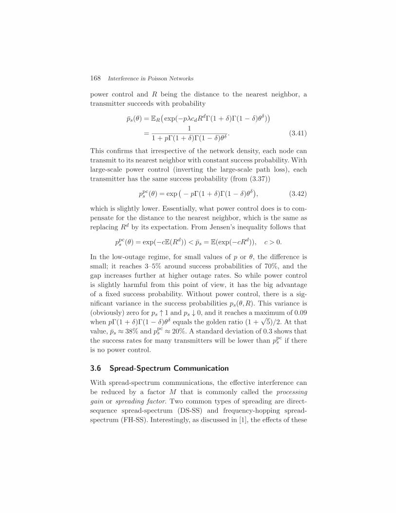
power control and R being the distance to the nearest neighbor, atransmitter succeeds with probability
ps(θ) = ER
(exp(−pλcdRdΓ(1 + δ)Γ(1 − δ)θδ)
)=
11 + pΓ(1 + δ)Γ(1 − δ)θδ . (3.41)
This confirms that irrespective of the network density, each node cantransmit to its nearest neighbor with constant success probability. Withlarge-scale power control (inverting the large-scale path loss), eachtransmitter has the same success probability (from (3.37))
ppcs (θ) = exp
(− pΓ(1 + δ)Γ(1 − δ)θδ
), (3.42)
which is slightly lower. Essentially, what power control does is to com-pensate for the distance to the nearest neighbor, which is the same asreplacing Rd by its expectation. From Jensen’s inequality follows that
ppcs (θ) = exp(−cE(Rd)) < ps = E(exp(−cRd)), c > 0.
In the low-outage regime, for small values of p or θ, the difference issmall; it reaches 3–5% around success probabilities of 70%, and thegap increases further at higher outage rates. So while power controlis slightly harmful from this point of view, it has the big advantageof a fixed success probability. Without power control, there is a sig-nificant variance in the success probabilities ps(θ,R). This variance is(obviously) zero for ps ↑ 1 and ps ↓ 0, and it reaches a maximum of 0.09when pΓ(1 + δ)Γ(1 − δ)θδ equals the golden ratio (1 +
√5)/2. At that
value, ps ≈ 38% and ppcs ≈ 20%. A standard deviation of 0.3 shows that
the success rates for many transmitters will be lower than ppcs if there
is no power control.
3.6 Spread-Spectrum Communication
With spread-spectrum communications, the effective interference canbe reduced by a factor M that is commonly called the processinggain or spreading factor. Two common types of spreading are direct-sequence spread-spectrum (DS-SS) and frequency-hopping spread-spectrum (FH-SS). Interestingly, as discussed in [1], the effects of these

3.7 CSMA and Interference Cancellation 169
techniques on the interference and outage are quite different, althoughthey both require an M -fold increase in system bandwidth.
With DS-SS, all transmitting nodes still cause interference, but theinterference is scaled by a factor M . The outage in Rayleigh fading isaffected by a reduction of the SIR threshold θ by a factor of M since
pDSs (θ,M) = E(e−θI/M ) = ps(θ/M).
So, from (3.29), we see that
DH-SS:logps(θ/M)
logps(θ)= M−δ.
On the other hand, with FH-SS, the density of interferers is reducedby a factor of M , which implies
FH-SS:logpFH
s (θ)logps(θ)
= M−1.
Since δ < 1, the benefit of FH-SS is larger; the difference is more drasticfor small δ, i.e., if the path loss exponent is large relative to the numberof network dimensions. More details are available in [1].
3.7 CSMA and Interference Cancellation
3.7.1 CSMA
Channel access schemes that are based on carrier sensing aim at upperbounding the interference at a receiver by prohibiting nearby nodesto transmit. The effect of CSMA-type MAC schemes on the interfer-ence can be investigated by calculating the residual interference thatstems from the transmitters outside the receiver’s carrier sensing range.Assuming a carrier sensing range of ρ, we obtain the Laplace transformof the residual interference using a modified path loss law
(r) = r−α1r>ρ,
and following the same steps as in the calculation of the entire inter-ference. In the non-fading case,
LI(s) = exp− λcd(sδγ(1 − δ,sρ−α) − ρd(1 − exp(−sρ−α)))
,
(3.43)
170 Interference in Poisson Networks
where γ(a,z) =∫ z0 exp(−t)ta−1dt is the lower incomplete gamma func-
tion. Since γ(a,z) < Γ(a) for finite z, this is larger than the Laplacetransform of the complete interference, as expected. For ρ > 0, the meanand variance are finite and given by
E(I) = − dds
log(LI(s))∣∣s=0 =
λcdd
α − dρd−α. (3.44)
var(I) =d2
ds2log(LI(s))
∣∣s=0 =
λcdd
2α − dρd−2α. (3.45)
These results follow from the fact that
lims→0
γ(1 − δ,sρ−α)s1−δ =
ρd−α
1 − δ .
In the fading case,
LI(s) =
exp− λcd(sδEh(hδγ(1 − δ,shρ−α)) − ρdEh(1 − exp(−shρ−α)))
.
The expectation of the term with the incomplete gamma function canbe evaluated numerically, or bounds can be used. In Rayleigh fading,the expectation of the exponential part is ρds/(s + ρα), and for δ = 1/2,
Eh(hδγ(1 − δ,shc)) =π
2− arctan
(1√sc
)+√sc
sc + 1.
Hence for Rayleigh fading and δ = 1/2,
LI(s) =
exp
−λcd
√s
(π
2− arctan
( 1√sρ−α
)+
√sρ−α
sρ−α + 1
)+λcdρ
ds
s + ρα
,
(3.46)
which confirms that the interference does not have a heavy tail forρ > 0.
Interpreting LI(θ) as the success probability in Rayleigh fading,the impact of CSMA on the outage can be quantified. Figure 3.4 showsthe success probability for ρ = 1/2,1,2 and ALOHA, for comparison.Strictly speaking, this formula is only an approximation, since the set
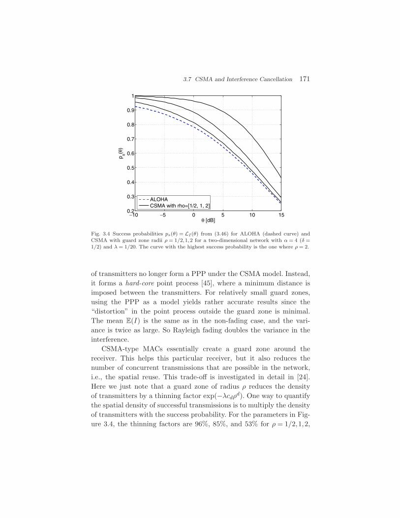
3.7 CSMA and Interference Cancellation 171
−10 −5 0 5 10 150.2
0.3
0.4
0.5
0.6
0.7
0.8
0.9
1
θ [dB]
p s(θ)
ALOHACSMA with rho=[1/2, 1, 2]
Fig. 3.4 Success probabilities ps(θ) = LI(θ) from (3.46) for ALOHA (dashed curve) andCSMA with guard zone radii ρ = 1/2,1,2 for a two-dimensional network with α = 4 (δ =1/2) and λ = 1/20. The curve with the highest success probability is the one where ρ = 2.
of transmitters no longer form a PPP under the CSMA model. Instead,it forms a hard-core point process [45], where a minimum distance isimposed between the transmitters. For relatively small guard zones,using the PPP as a model yields rather accurate results since the“distortion” in the point process outside the guard zone is minimal.The mean E(I) is the same as in the non-fading case, and the vari-ance is twice as large. So Rayleigh fading doubles the variance in theinterference.
CSMA-type MACs essentially create a guard zone around thereceiver. This helps this particular receiver, but it also reduces thenumber of concurrent transmissions that are possible in the network,i.e., the spatial reuse. This trade-off is investigated in detail in [24].Here we just note that a guard zone of radius ρ reduces the densityof transmitters by a thinning factor exp(−λcdρd). One way to quantifythe spatial density of successful transmissions is to multiply the densityof transmitters with the success probability. For the parameters in Fig-ure 3.4, the thinning factors are 96%, 85%, and 53% for ρ = 1/2,1,2,

172 Interference in Poisson Networks
respectively. For ρ = 1, the product of success probability and densityof transmitters is higher than in the ALOHA case as soon as θ > 0dB. Generally, the optimum width of the guard zone depends on thereliability and energy efficiency requirements.
In [37], the authors analyzed the performance of CSMA in dense802.11 networks. They used a Matern-type hard-core process to modelthe impact of CSMA on the node distribution.
3.7.2 Interference Cancellation
Multi-user receivers can achieve significantly higher performance inwireless networks. Successive interference cancellation (SIC) is a par-ticularly appealing technique when the received powers from the usersdiffer greatly [47, 38]. In a large wireless network, one can expect sub-stantial benefits if the interference from one or a few of the strongestinterferers can be canceled. A similar effect as in CSMA can beachieved, albeit without the reduction in transmitter density. We havepreviously derived an expression for the distribution of the interfer-ence from each individual interferer (3.26); however, using this resultin the present context is complicated by the fact that the distance dis-tributions are not independent. The tail probabilities of the individualinterference powers (3.27) tell us how heavy the tail remains if a certainnumber of nearby interferers are canceled, but again this does not helpwith analyzing the outage probabilities.
The Laplace transforms of the interference from the nearest n trans-mitters is given in (3.19) for Rayleigh fading and δ = 1/2. Let ps(θ,I),I ⊂ N, be the success probability if the i-th nearest interferers, i ∈ I,are present and active. From ps(θ, [n]) = LIn(θ) we define as the n-thinterferer’s contribution to the outage
ps(θ,n) ps(θ, [n])ps(θ, [n − 1])
.
and the success probability when the k nearest interferers are canceled,
ps(θ,N \ [k]) ps(θ,N)ps(θ, [k])
.
Using (3.19), these probabilities can easily be found numerically. Fig-ure 3.5 (left) shows the success probabilities for k = 0 (no SIC) and
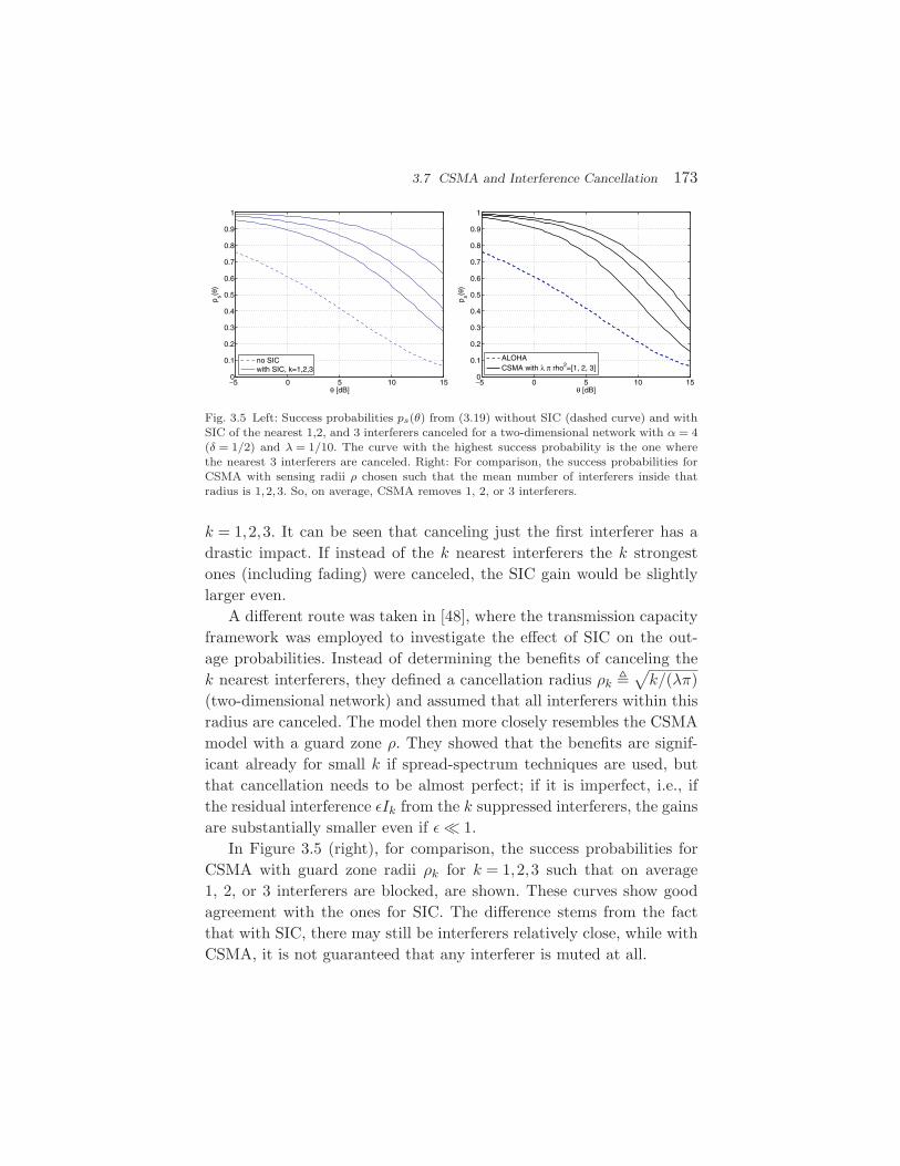
3.7 CSMA and Interference Cancellation 173
−5 0 5 10 150
0.1
0.2
0.3
0.4
0.5
0.6
0.7
0.8
0.9
1
θ [dB]
p s(θ)
no SICwith SIC, k=1,2,3
−5 0 5 10 150
0.1
0.2
0.3
0.4
0.5
0.6
0.7
0.8
0.9
1
θ [dB]
p s(θ)
ALOHACSMA with λ π rho2=[1, 2, 3]
Fig. 3.5 Left: Success probabilities ps(θ) from (3.19) without SIC (dashed curve) and withSIC of the nearest 1,2, and 3 interferers canceled for a two-dimensional network with α = 4(δ = 1/2) and λ = 1/10. The curve with the highest success probability is the one wherethe nearest 3 interferers are canceled. Right: For comparison, the success probabilities forCSMA with sensing radii ρ chosen such that the mean number of interferers inside thatradius is 1,2,3. So, on average, CSMA removes 1, 2, or 3 interferers.
k = 1,2,3. It can be seen that canceling just the first interferer has adrastic impact. If instead of the k nearest interferers the k strongestones (including fading) were canceled, the SIC gain would be slightlylarger even.
A different route was taken in [48], where the transmission capacityframework was employed to investigate the effect of SIC on the out-age probabilities. Instead of determining the benefits of canceling thek nearest interferers, they defined a cancellation radius ρk
√k/(λπ)
(two-dimensional network) and assumed that all interferers within thisradius are canceled. The model then more closely resembles the CSMAmodel with a guard zone ρ. They showed that the benefits are signif-icant already for small k if spread-spectrum techniques are used, butthat cancellation needs to be almost perfect; if it is imperfect, i.e., ifthe residual interference εIk from the k suppressed interferers, the gainsare substantially smaller even if ε 1.
In Figure 3.5 (right), for comparison, the success probabilities forCSMA with guard zone radii ρk for k = 1,2,3 such that on average1, 2, or 3 interferers are blocked, are shown. These curves show goodagreement with the ones for SIC. The difference stems from the factthat with SIC, there may still be interferers relatively close, while withCSMA, it is not guaranteed that any interferer is muted at all.
174 Interference in Poisson Networks
3.8 Interference Correlation
From the previous section we observe that the interference distribu-tion in a Poisson network does not depend on the spatial location dueto the stationarity of the PPP. Even though the interference distribu-tion is identical on the entire plane (in the two-dimensional case), theinterference is not independent across the plane. This is because theinterference is caused by common randomness, namely the point pro-cess Φ. The spatial and temporal correlation of the interference is oftenignored in the literature, or removed by the assumption that a newrealization of the point process is drawn in each time slot [46]. This isclearly not the case in practical networks, and thus there is a need toanalyze the correlation structure of the interference if the point processrealization does not change. This is the topic of this section.
Since each node in a wireless network uses a MAC protocol to decidewhether to transmit or receive, the transmitting set in time slot k,denoted as Φk, changes with time k but is always a subset of Φ; asa consequence, the interference becomes correlated over time becauseof the common randomness Φ. In this section we consider ALOHAas the MAC protocol in which each node transmits with probabilityp and receive with 1 − p independently of other nodes. We observethat ALOHA as a MAC protocol introduces no correlations since thetransmitters are independently chosen in space and time. Neverthelessthe presence of the common randomness Φ causes the interference tobe temporally correlated.
When (x) = ‖x‖−α the interference is heavy-tailed with parame-ter 2/α. As mentioned earlier the average interference and the highermoments are not finite since an interfering transmitter can be very closeto the origin (where the interference is calculated). The correlation coef-ficient cannot be defined when the moments are not finite. Hence weuse a bounded path loss model and calculate the spatio-temporal cor-relation coefficient for (x) = ‖x‖−α as a limiting case.
(x) is assumed to have the following properties:
(1) Depends only on ‖x‖.(2) Monotonically decreases with ‖x‖.
3.8 Interference Correlation 175
(3) Integrable: ∫ ∞
0x(x)dx <∞. (3.47)
For example, a valid path loss model is given by
ε(x) =1
ε + ‖x‖α , ε ∈ (0,∞), α > 2. (3.48)
The standard singular path loss model (x) = ‖x‖−α is obtained bytaking the limit limε→0 ε(x). Since in ALOHA, each node makes anindependent decision to transmit at every time instant, the set of trans-mitters at a time instant is a thinned version of the original PPP Φ,and the resulting transmitter process at time instant k, Φk, is again aPPP. This can be easily verified by considering the void probability:For any bounded set B ⊂ R
2, we have
P(Φk(B) = 0) = E
∏x∈Φ∩B
1(x not a transmitter at time k)
(a)=
∏x∈Φ∩B
P(x not a transmitter at time k)
= E[(1 − p)Φ(B)](b)= exp(−λp|B|).
(a) follows since each node decides to not transmit independently fromeach other. Since Φ is a PPP, Φ(B) is a Poisson random variable withmean λ|B|, (b) follows from the moment generating function of thePoisson random variable. From the above we see that the void prob-ability of the transmitting process at time k is exp(−pλ|B|), whichcorresponds to that of a PPP. We also observe that Φk has densitypλ which is intuitive. The interference at time instant k and (spatial)location z is given by
Ik(z) =∑x∈Φ
1(x ∈ Φk)hxz(k)(x − z). (3.49)
We assume that the fading is independent across time (block fading)and space.
176 Interference in Poisson Networks
3.8.1 Spatio-Temporal Correlation of the Interference
We calculate the correlation coefficient of the random variables, Ik(u)and Il(v),k = l,u = v. In order to calculate the joint moments of therandom variables, the joint Laplace transform of the random variablesIk(u) and Il(v) will be used.
Theorem 3.1. The joint Laplace transform of Ik(u) and Il(v), k = l, is
L(s1,s2) = exp(−λ
∫R2
[1 − ξ(s1,u − x)ξ(s2,v − x)]dx),
where
ξ(s,x) = 1 − p + pLh(s(x)),
and Lh denotes the Laplace transform of the fading process.
Proof. The interference at time k and location u ∈ R2 is given by
Ik(u) =∑x∈Φk
hxu(k)(x − u),
and the interference at v ∈ R2 at time l is
Il(v) =∑y∈Φl
hyv(l)(y − v).
So the joint Laplace transform is
L(s1,s2) = Eexp
−s1 ∑
x∈Φk
hxu(k)(x − u) − s2∑y∈Φl
hyv(l)(y − v)
.
Rewriting this as a product,
L(s1,s2) = E
∏x∈Φ
exp(−s11(x ∈ Φk)hxu(k)(x − u))
× exp(−s21(x ∈ Φl)hxv(l)(x − v)).Since in ALOHA each node decides to transmit independently of othernodes and across time, taking the expectation with respect to ALOHA,
L(s1,s2) = E
∏x∈Φ
[1 − p + pexp(−s1hxu(k)(x − u))]
× [1 − p + pexp(−s2hxv(l)(x − v))].
3.8 Interference Correlation 177
Since fading is assumed to be independent across time and space, mov-ing the expectation with respect to fading inside we get
L(s1,s2) = E
∏x∈Φ
[1 − p + pLh(s1(x − u))][1 − p + pLh(s2(x − v))]
= E
∏x∈Φ
ξ(s1,x − u)ξ(s2,x − v)
(c)= exp(−λ
∫R2
[1 − ξ(s1,x − u)ξ(s2,x − v)]dx).
The last step follows from the PGFL of the PPP (A.3).
The above proof can be generalized to obtain the joint Laplacetransform of the m random variables Ik1(u1), . . . , Ikm(um), k1 =k2, . . . , = km and u1 = u2, . . . , = um:
LIK(s1, . . . ,sm) = exp
(−λ
∫R2
[1 −
m∏i=1
ξ(si,x − ui)]
dx
).
In the above theorem, we have considered the interference at two dif-ferent time slots and at different spatial locations.
By a similar approach as in the theorem above, the joint Laplacetransform of the random variables Ik(u) and Ik(v), i.e., interference atthe same time instant but at different locations can be shown to be
LI(u)I(k)(s1,s2) = exp(−λ
∫R2
[1 − Lh(s1(x − u))Lh(s2(x − v))]dx).
(3.50)The mean of the interference is
EIk(u) = − ∂
∂s1L(s1,0)
∣∣∣s1=0
= − ∂
∂s1exp
(−λ
∫R2
[1 − ξ(s1,x − u)ξ(0,x − v)]dx)∣∣∣
s1=0
= λp
∫R2
∂
∂s1Lh(s1(x − u))dx
∣∣∣s1=0
= pλE[h]∫
R2(x − u)dx
= pλ
∫R2(x)dx, (3.51)
178 Interference in Poisson Networks
since E[h] = 1. The second moment of the interference is
E[Ik(u)2] =∂2
∂2s1L(s1,0)
∣∣∣s1=0
,
and by simple algebraic manipulations, the second moment
E[Ik(u)2] = pE[h2]λ∫
R22(x)dx
+p2E[h]2λ2
∫R2
∫R2(x)(y)dxdy. (3.52)
is obtained. When the path loss is given by ε(x) and the fading isRayleigh, we can use the above theorem to obtain the Laplace transformof the interference as
LIΦ(s) = exp(−πλps(ε + s)δ−1 πδ
sin(πδ)
),
where δ = 2/α.The mean and the variance do not depend on either the position or
the time index. When the fading follows a Nakagami-m distribution andthe path loss model is given by ε(x), the variance of the interferencefollows from (3.51) and (3.52) and is given by
var[Ik(u)] =pλπ
ε2−δπδ
sin(πδ)(1 − δ)(1 + m−1).
We observe that the variance is maximum, when the fading is Rayleighand the minimum exactly half of the maximum when there is no fading(i.e., m =∞). As expected, the mean and the variance diverge whenε = 0. The mean of the product of Ik(u) and Il(v) at times k and l, k = l,which is required for the calculation of the correlation coefficient, is
E[Ik(u)Il(v)] =∂2
∂s2∂s1L(s1,s2)
∣∣∣(s1,s2)=(0,0)
= p2λ
∫R2(x − u)(x − v)dx + λ2p2
(∫R2(x)dx
)2
.
Lemma 3.2. The spatio-temporal correlation coefficient of the inter-ferences Ik(u) and Il(v), k = l, for ALOHA and path loss functions (x)

3.8 Interference Correlation 179
satisfying (3.47) is
ζ(u,v) =p∫
R2 (x)(x − ‖u − v‖)dxE[h2]
∫R2 2(x)dx
. (3.53)
Proof. Since Ik(u) and Il(v) are identically distributed, we have
ζ(u,v) =E[Ik(u)Il(v)] − E[Ik(u)]2
E[Ik(u)2] − E[Ik(u)]2.
By substituting for the above quantities we have
ζ(u,v) =p∫
R2 (x − u)(x − v)dxE[h2]
∫R2 2(x)dx
(a)=
p∫
R2 (x)(x − ‖u − v‖)dxE[h2]
∫R2 2(x)dx
, (3.54)
where (a) follows by substituting y = x − u and the fact that (x)depends only on ‖x‖.
We observe that the correlation coefficient does not depend on k
and l and is equal for any two time instants. From (3.50) we obtain thefollowing lemma on the spatial correlation:
Lemma 3.3. The spatial correlation coefficient of the interference, i.e.,the correlation coefficient of Ik(u) and Ik(v), u = v is
ζs(u,v) =
∫R2 (x)(x − ‖u − v‖)dx
E[h2]∫
R2 2(x)dx. (3.55)
By setting ‖u − v‖ = 0 in Lemma 3.2, we obtain the temporal correla-tion coefficient:
Lemma 3.4. The temporal correlation coefficient for ALOHA is
ζt =p
E[h2], (3.56)
independent of (x). When the fading is Nakagami-m, the correlationcoefficient is ζt = pm
m+1 . In particular, for m = 1 (Rayleigh fading), the
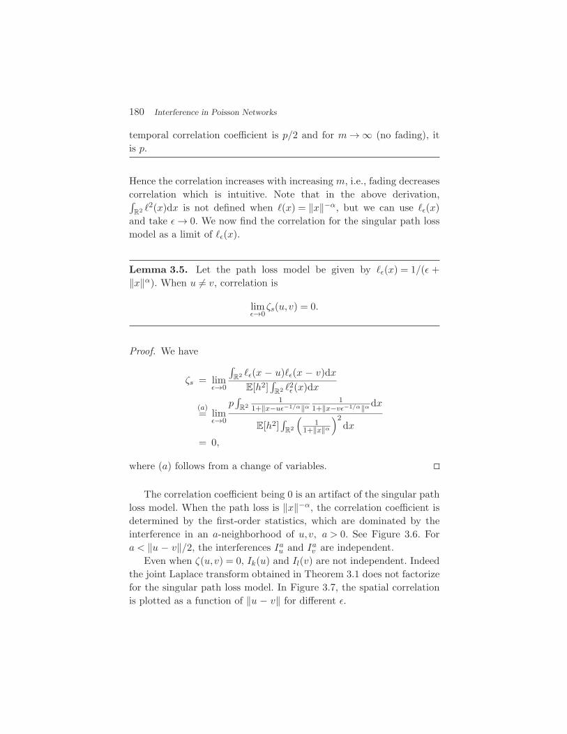
180 Interference in Poisson Networks
temporal correlation coefficient is p/2 and for m→∞ (no fading), itis p.
Hence the correlation increases with increasing m, i.e., fading decreasescorrelation which is intuitive. Note that in the above derivation,∫
R2 2(x)dx is not defined when (x) = ‖x‖−α, but we can use ε(x)
and take ε→ 0. We now find the correlation for the singular path lossmodel as a limit of ε(x).
Lemma 3.5. Let the path loss model be given by ε(x) = 1/(ε +‖x‖α). When u = v, correlation is
limε→0
ζs(u,v) = 0.
Proof. We have
ζs = limε→0
∫R2 ε(x − u)ε(x − v)dx
E[h2]∫
R2 2ε (x)dx
(a)= lim
ε→0
p∫
R21
1+‖x−uε−1/α‖α1
1+‖x−vε−1/α‖α dx
E[h2]∫
R2
(1
1+‖x‖α
)2dx
= 0,
where (a) follows from a change of variables.
The correlation coefficient being 0 is an artifact of the singular pathloss model. When the path loss is ‖x‖−α, the correlation coefficient isdetermined by the first-order statistics, which are dominated by theinterference in an a-neighborhood of u,v, a > 0. See Figure 3.6. Fora < ‖u − v‖/2, the interferences Iau and Iav are independent.
Even when ζ(u,v) = 0, Ik(u) and Il(v) are not independent. Indeedthe joint Laplace transform obtained in Theorem 3.1 does not factorizefor the singular path loss model. In Figure 3.7, the spatial correlationis plotted as a function of ‖u − v‖ for different ε.
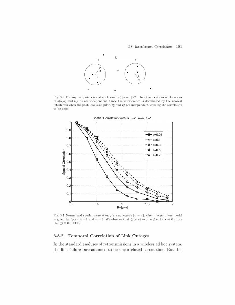
3.8 Interference Correlation 181
a
auv
R
Fig. 3.6 For any two points u and v, choose a < ‖u − v‖/2. Then the locations of the nodesin b(u,a) and b(v,a) are independent. Since the interference is dominated by the nearestinterferers when the path loss is singular, Ia
u and Iav are independent, causing the correlation
to be zero.
0 0.5 1 1.5 20
0.1
0.2
0.3
0.4
0.5
0.6
0.7
0.8
0.9
1
R=|u–v|
Spa
tial C
orre
latio
n
Spatial Correlation versus |u–v|, α=4, λ =1
ε=0.01
ε=0.1
ε=0.3
ε=0.5
ε=0.7
Fig. 3.7 Normalized spatial correlation ζ(u,v)/p versus ‖u − v‖, when the path loss modelis given by ε(x), λ = 1 and α = 4. We observe that ζs(u,v) → 0, u = v, for ε → 0 (from[14] c© 2009 IEEE).
3.8.2 Temporal Correlation of Link Outages
In the standard analyses of retransmissions in a wireless ad hoc system,the link failures are assumed to be uncorrelated across time. But this

182 Interference in Poisson Networks
is not so, since the interference is temporally correlated. We now pro-vide the conditional probability of link formation assuming a successfultransmission.
We assume that a transmitter at the origin has a destination locatedat z ∈ R
2. Let Ak denote the event that the origin is able to connectto its destination z at time instant k, i.e.,
SIR =hoz(k)(z)Ik(z)
> θ.
For simplicity we shall assume the fading is Rayleigh (similar methodscan be used for Nakagami-m). We now provide the joint probability ofsuccess P(Ak,Al), k = l. We have
P(Ak,Al)
= P(hoz(k) > θzIk(z),hoz(l) > θzIl(z))
(a)= E [exp(−θzIk(z))exp(−θzIl(z))]
= E
[exp
(−θz
∑x∈Φ
(x)[1(x ∈ Φk)hxz(k) + 1(x ∈ Φl)hxz(l)]
)]
(b)= E
[∏x∈Φ
(p
1 + θz(x)+ 1 − p
)2]
(c)= exp
(−λ
∫R2
1 −(
p
1 + θz(x)+ 1 − p
)2
dx
), (3.57)
where θz = θ/(z). (a) follows from the independence of hoz(k) andhoz(l), k = l, (b) follows by taking the average with respect tohxz(k), hxz(l) and ALOHA, (c) follows from the probability generatingfunctional of the PPP. Similarly, we have
P(Al) = exp(−λ
∫R2
1 −(
p
1 + θz(x)+ 1 − p
)dx).
Hence the conditional probability is
P(Ak | Al) = exp
(−λ
∫R2
pθz(x)1 + θz(x)
−(
pθz(x)1 + θz(x)
)2
dx
).

3.8 Interference Correlation 183
The ratio of conditional and the unconditional probability is given by
P(Ak | Al)P(Al)
=P(Ak,Al)P(Al)2
= exp
(λp2
∫R2
(θz(x)
1 + θz(x)
)2
dx
).
> 1. (3.58)
When (x) = ‖x‖−α, we have
P(Ak | Al)P(Al)
= exp(p2λπ‖z‖2(1 − δ) πδ
sin(πδ)θδ),
where δ = 2/α. In Figures 3.8 and 3.9, we plot the conditional and theunconditional link success probabilities versus the ALOHA parameter,p and z, respectively.
0 0.2 0.4 0.6 0.8 10.2
0.3
0.4
0.5
0.6
0.7
0.8
0.9
1
p
α=4, λ =1, θ=1, z=0.5
Unconditional: P(Al)
Conditional: P(Ak|A
l)
Fig. 3.8 P(Ak | Al) and P(Al) versus the ALOHA parameter p. λ = 1, (x) = ‖x‖−4, z = 0.5,θ = 1 (from [14] c© 2009 IEEE).

184 Interference in Poisson Networks
0 0.5 1 1.50
0.1
0.2
0.3
0.4
0.5
0.6
0.7
0.8
0.9
1
z
α=4, λ =1, θ=1, z=0.5
Unconditional: P(Al)
Conditional: P(Ak|A
l)
Conditional:P(Ak|A
lc)
Fig. 3.9 P(Ak | Al) and P(Al) versus the distance z. λ = 1, (x) = ‖x‖−4, p = 0.5, θ = 1.
We make the following observations:
(1) The link formation is correlated across time (see (3.58)).(2) If a transmission succeeds at a time instant k, there is a
higher probability that a transmission succeeds at a timeinstant l.
(3) From (3.58), we also have P(Ack|Acl ) > P(Acl ). So a link in out-age is always more likely to be in outage; hence the retrans-mission strategy should reduce the rate of transmission orchange the density of transmitters rather than retransmit“blindly”.
(4) P(Ak|Al)P(Al)
always increases with θ,λ,p, and ‖z‖. The increasein λ and p is because of the larger transmit set due to whichthe probability of the same subset of nodes transmitting atdifferent times increases, thereby causing more correlation.When θ is large, the outage is a result of the interfering
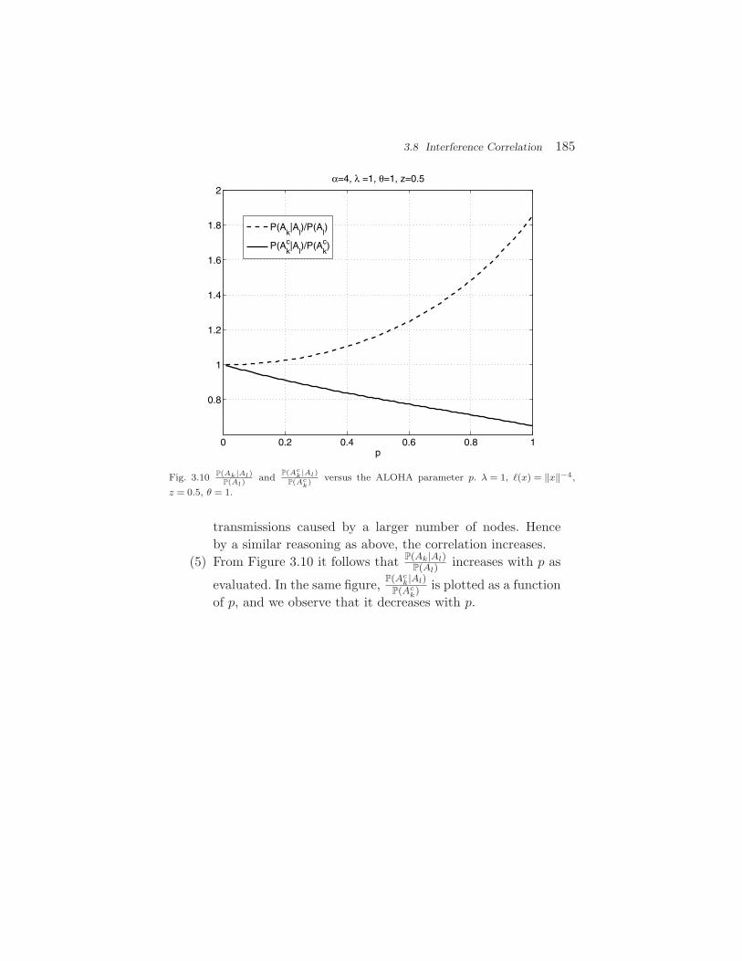
3.8 Interference Correlation 185
0 0.2 0.4 0.6 0.8 1
0.8
1
1.2
1.4
1.6
1.8
2
p
α=4, λ =1, θ=1, z=0.5
P(Ak|A
l)/P(A
l)
P(Akc|A
l)/P(A
kc)
Fig. 3.10 P(Ak|Al)P(Al)
and P(Ack|Al)
P(Ack) versus the ALOHA parameter p. λ = 1, (x) = ‖x‖−4,
z = 0.5, θ = 1.
transmissions caused by a larger number of nodes. Henceby a similar reasoning as above, the correlation increases.
(5) From Figure 3.10 it follows that P(Ak|Al)P(Al)
increases with p as
evaluated. In the same figure, P(Ack|Al)
P(Ack) is plotted as a function
of p, and we observe that it decreases with p.
4Interference in Poisson Cluster Networks
In the previous section we have analyzed the interference when theunderlying transmitter set is a PPP. While this may be the case forcertain networks, it is much more likely that the node distribution isnot “completely spatially random” (CSR), i.e., that nodes are eitherclustered or more regularly distributed. Moreover, even if the completeset of nodes constitutes a PPP, the subset of active nodes may notbe homogeneously Poisson. Instead, the transmitting node set may beclustered or regularly arranged (see Section 2).
The clustering of transmitting nodes may be due to geographicalfactors; for example, in a social gathering, people tend to cluster intosmall groups, or in a battlefield, the soldiers move in small groups in acoordinated fashion, or in a down-town region, wireless nodes are clus-tered in buildings, or in a cognitive network, the active cognitive userstend to be clustered. The clustering may also be “artificially” inducedby MAC protocols. We denote the former as geographical clusteringand the latter as logical clustering. See Figure 4.1. Also the benefits ofrandomly arranged transmissions as compared to clustered transmis-sions are not a priori clear. In this section we analyze the interferenceand outage properties when the transmitters are clustered as a Poisson
186
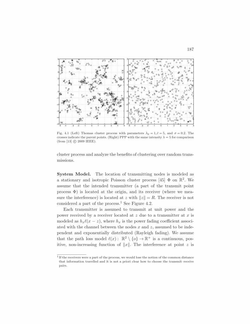
187
−5 −4 −3 −2 −1 0 1 2 3 4 5−5
−4
−3
−2
−1
0
1
2
3
4
5
−5 −4 −3 −2 −1 0 1 2 3 4 5−5
−4
−3
−2
−1
0
1
2
3
4
5
Fig. 4.1 (Left) Thomas cluster process with parameters λp = 1, c = 5, and σ = 0.2. Thecrosses indicate the parent points. (Right) PPP with the same intensity λ = 5 for comparison(from [13] c© 2009 IEEE).
cluster process and analyze the benefits of clustering over random trans-missions.
System Model. The location of transmitting nodes is modeled asa stationary and isotropic Poisson cluster process [45] Φ on R
2. Weassume that the intended transmitter (a part of the transmit pointprocess Φ) is located at the origin, and its receiver (where we mea-sure the interference) is located at z with ‖z‖ = R. The receiver is notconsidered a part of the process.1 See Figure 4.2.
Each transmitter is assumed to transmit at unit power and thepower received by a receiver located at z due to a transmitter at x ismodeled as hx(x − z), where hx is the power fading coefficient associ-ated with the channel between the nodes x and z, assumed to be inde-pendent and exponentially distributed (Rayleigh fading). We assumethat the path loss model (x) : R
2 \ o → R+ is a continuous, pos-
itive, non-increasing function of ‖x‖. The interference at point z is
1 If the receivers were a part of the process, we would lose the notion of the common distancethat information travelled and it is not a priori clear how to choose the transmit–receivepairs.
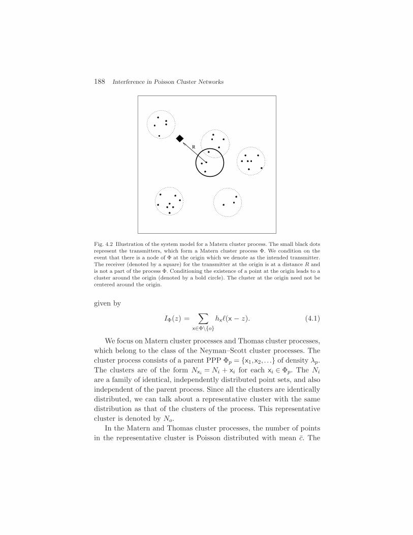
188 Interference in Poisson Cluster Networks
R
Fig. 4.2 Illustration of the system model for a Matern cluster process. The small black dotsrepresent the transmitters, which form a Matern cluster process Φ. We condition on theevent that there is a node of Φ at the origin which we denote as the intended transmitter.The receiver (denoted by a square) for the transmitter at the origin is at a distance R andis not a part of the process Φ. Conditioning the existence of a point at the origin leads to acluster around the origin (denoted by a bold circle). The cluster at the origin need not becentered around the origin.
given by
IΦ(z) =∑
x∈Φ\ohx(x − z). (4.1)
We focus on Matern cluster processes and Thomas cluster processes,which belong to the class of the Neyman–Scott cluster processes. Thecluster process consists of a parent PPP Φp = x1,x2, . . . of density λp.The clusters are of the form Nxi = Ni + xi for each xi ∈ Φp. The Ni
are a family of identical, independently distributed point sets, and alsoindependent of the parent process. Since all the clusters are identicallydistributed, we can talk about a representative cluster with the samedistribution as that of the clusters of the process. This representativecluster is denoted by No.
In the Matern and Thomas cluster processes, the number of pointsin the representative cluster is Poisson distributed with mean c. The

189
daughter points of the representative cluster No are scattered indepen-dently and with a identical spatial distribution
Fcl(A) =∫Afcl(x)dx, A ⊂ R
2,
around the origin. For the Matern cluster process each point is uni-formly distributed in a ball of radius a around the origin. So the densityfunction fcl(x) is given by
fcl(x) =
1πa2 , ‖x‖ ≤ a0 otherwise.
(4.2)
In the Thomas cluster process, each point is scattered using a sym-metric normal distribution with variance σ2 around the origin. So thedensity function fcl(x) is given by
fcl(x) =1
2πσ2 exp(−‖x‖
2
2σ2
).
The complete process Φ is given by
Φ =⋃
x∈Φp
Nx,
and the PGFL is (see (A.4))
G[ν] E
[∏x∈Φ
ν(x)
]
= exp(−λp
∫Rd
1 −M(∫
Rd
ν(x + y)fcl(x)dx))
,
where M(z) = exp(c(z − 1)). The second-order product density of theMatern and the Thomas cluster processes [45, Section 5.3] is
ρ(2)(z) = λpc2[(fcl ∗ fcl)(z) + λp]. (4.3)
See Section A.1.3 and [45, Section 5.3] for a detailed description ofclustered point processes.

190 Interference in Poisson Cluster Networks
4.1 Interference Characterization
In this section, we will derive the statistical characteristics of the inter-ference when the transmitters are distributed as a PCP. As shall beevident in the next section, we will derive the interference propertiesconditioning on a transmitter being at the origin (the desired transmit-ter). Differently from the PPP, placing an additional transmitter at theorigin (even though it does not contribute to the interference) makesthe distribution of the interference non-stationary, i.e., the interferenceIΦ(z) distribution depends on z. The average interference (conditionedon the event that there is a point of the process at the origin) is
E!o[IΦ(z)] = E
!o
[∑x∈Φ
hx(x − z)]
= E[h]λ∫
R2(x − z)K2(dx), (4.4)
where K2 is the second-order moment measure (A.8) and E!o is the
expectation with respect to the reduced Palm measure. Equivalently,by the relation (A.9), we have
E!o[IΦ(z)] =
E[h]λ
∫R2(x − z)ρ(2)(x)dx. (4.5)
Example: Thomas Cluster Process. In this case, from [45, p. 160],
ρ(2)(x)λ2 = 1 +
14πλpσ2 exp
(−‖x‖24σ2
),
where λ = λpc. We obtain
E!o[IΦ(z)] = EIPoi (λ) +
cE[h]4πσ2
∫R2(x − z)exp
(−‖x‖24σ2
)dx. (4.6)
EIPoi (λ) is the average interference when the nodes are distributedas a PPP with intensity λ. EIPoi (λ) is finite only when (x) is boundedat the origin. The above expression also shows that the mean inter-ference is indeed larger than for the PPP, and that E
!o[IΦ(z)]→ EIPoi
when ‖z‖ →∞, which is intuitive since the effect of the cluster at theorigin vanishes as ‖z‖ increases. We now derive the conditional Laplacetransform of the interference. First we show that it can be expressedusing the conditional PGFL of Φ.
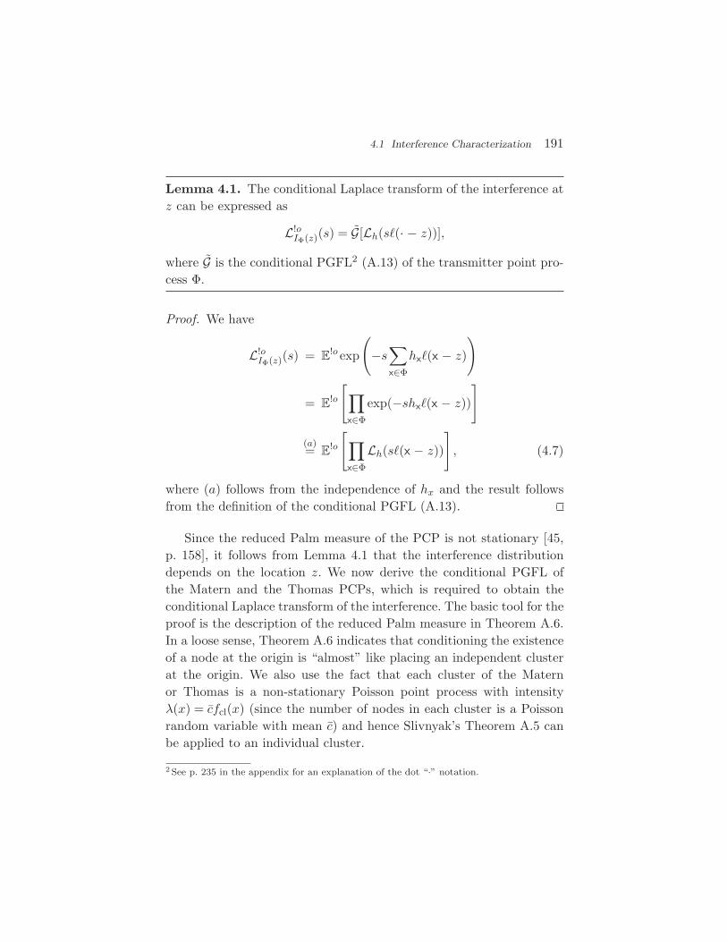
4.1 Interference Characterization 191
Lemma 4.1. The conditional Laplace transform of the interference atz can be expressed as
L!oIΦ(z)(s) = G[Lh(s(· − z))],
where G is the conditional PGFL2 (A.13) of the transmitter point pro-cess Φ.
Proof. We have
L!oIΦ(z)(s) = E
!o exp
(−s
∑x∈Φ
hx(x − z))
= E!o
[∏x∈Φ
exp(−shx(x − z))]
(a)= E
!o
[∏x∈Φ
Lh(s(x − z))], (4.7)
where (a) follows from the independence of hx and the result followsfrom the definition of the conditional PGFL (A.13).
Since the reduced Palm measure of the PCP is not stationary [45,p. 158], it follows from Lemma 4.1 that the interference distributiondepends on the location z. We now derive the conditional PGFL ofthe Matern and the Thomas PCPs, which is required to obtain theconditional Laplace transform of the interference. The basic tool for theproof is the description of the reduced Palm measure in Theorem A.6.In a loose sense, Theorem A.6 indicates that conditioning the existenceof a node at the origin is “almost” like placing an independent clusterat the origin. We also use the fact that each cluster of the Maternor Thomas is a non-stationary Poisson point process with intensityλ(x) = cfcl(x) (since the number of nodes in each cluster is a Poissonrandom variable with mean c) and hence Slivnyak’s Theorem A.5 canbe applied to an individual cluster.
2 See p. 235 in the appendix for an explanation of the dot “·” notation.
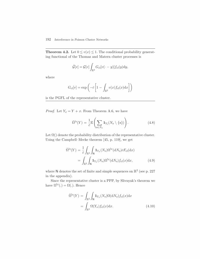
192 Interference in Poisson Cluster Networks
Theorem 4.2. Let 0 ≤ v(x) ≤ 1. The conditional probability generat-ing functional of the Thomas and Matern cluster processes is
G[v] = G[v]∫
R2Gcl[v(· − y)]fcl(y)dy,
where
Gcl[v] = exp(−c
[1 −
∫R2v(x)fcl(x)dx
])
is the PGFL of the representative cluster.
Proof. Let Yx = Y + x. From Theorem A.6, we have
Ω!o(Y ) =1cE
(∑x∈No
1Yx(No \ x)). (4.8)
Let Ω() denote the probability distribution of the representative cluster.Using the Campbell–Mecke theorem [45, p. 119], we get
Ω!o(Y ) =1c
∫R2
∫N1Yx(No)Ω!x(dNo)cFcl(dx)
=∫
R2
∫N1Yx(No)Ω!x(dNo)fcl(x)dx, (4.9)
where N denotes the set of finite and simple sequences on R2 (see p. 227
in the appendix).Since the representative cluster is a PPP, by Slivnyak’s theorem we
have Ω!x(.) = Ω(.). Hence
Ω!o(Y ) =∫
R2
∫N1Yx(No)Ω(dNo)fcl(x)dx
=∫
R2Ω(Yx)fcl(x)dx. (4.10)
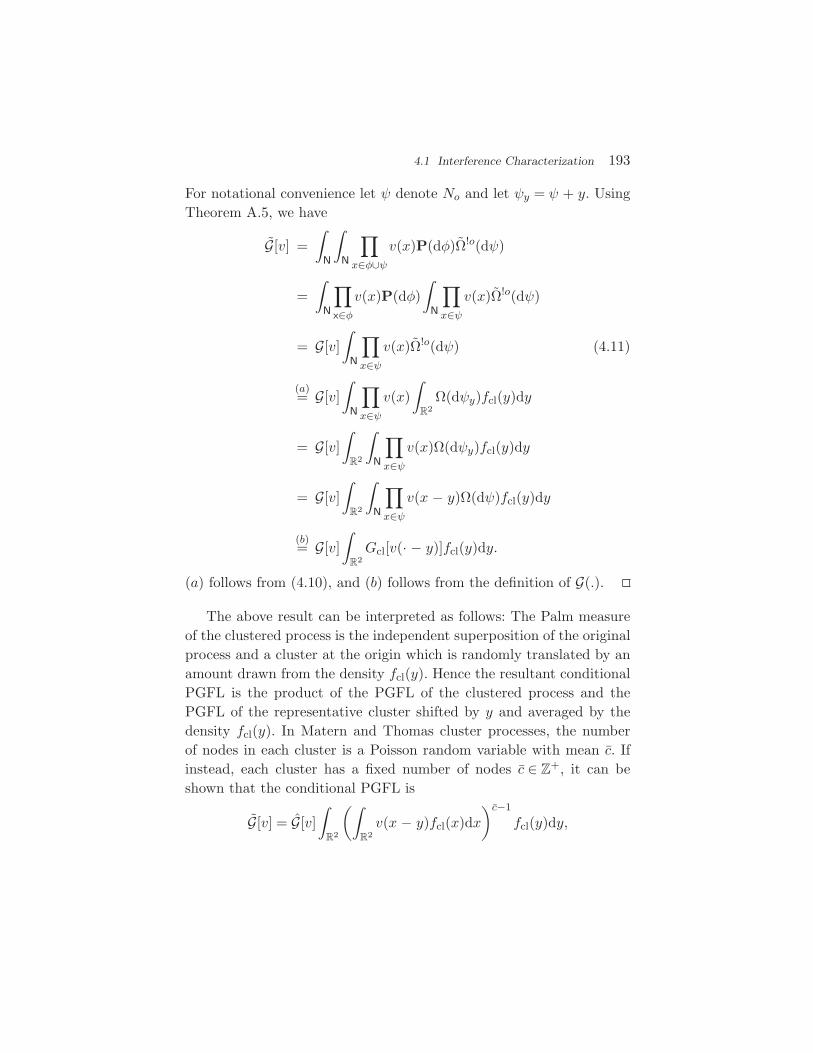
4.1 Interference Characterization 193
For notational convenience let ψ denote No and let ψy = ψ + y. UsingTheorem A.5, we have
G[v] =∫
N
∫N
∏x∈φ∪ψ
v(x)P(dφ)Ω!o(dψ)
=∫
N
∏x∈φ
v(x)P(dφ)∫
N
∏x∈ψ
v(x)Ω!o(dψ)
= G[v]∫
N
∏x∈ψ
v(x)Ω!o(dψ) (4.11)
(a)= G[v]
∫N
∏x∈ψ
v(x)∫
R2Ω(dψy)fcl(y)dy
= G[v]∫
R2
∫N
∏x∈ψ
v(x)Ω(dψy)fcl(y)dy
= G[v]∫
R2
∫N
∏x∈ψ
v(x − y)Ω(dψ)fcl(y)dy
(b)= G[v]
∫R2Gcl[v(· − y)]fcl(y)dy.
(a) follows from (4.10), and (b) follows from the definition of G(.).
The above result can be interpreted as follows: The Palm measureof the clustered process is the independent superposition of the originalprocess and a cluster at the origin which is randomly translated by anamount drawn from the density fcl(y). Hence the resultant conditionalPGFL is the product of the PGFL of the clustered process and thePGFL of the representative cluster shifted by y and averaged by thedensity fcl(y). In Matern and Thomas cluster processes, the numberof nodes in each cluster is a Poisson random variable with mean c. Ifinstead, each cluster has a fixed number of nodes c ∈ Z
+, it can beshown that the conditional PGFL is
G[v] = G[v]∫
R2
(∫R2v(x − y)fcl(x)dx
)c−1
fcl(y)dy,
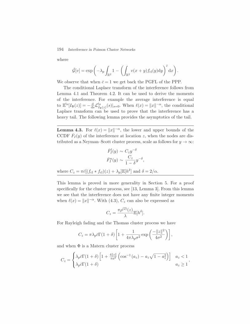
194 Interference in Poisson Cluster Networks
where
G[v] = exp(−λp
∫R2
1 −(∫
R2v(x + y)fcl(y)dy
)cdx).
We observe that when c = 1 we get back the PGFL of the PPP.The conditional Laplace transform of the interference follows from
Lemma 4.1 and Theorem 4.2. It can be used to derive the momentsof the interference. For example the average interference is equalto E
!o[IΦ(z)] = − ddsL!o
IΦ(z)(s)|s=0. When (x) = ‖x‖−α, the conditionalLaplace transform can be used to prove that the interference has aheavy tail. The following lemma provides the asymptotics of the tail.
Lemma 4.3. For (x) = ‖x‖−α, the lower and upper bounds of theCCDF FI(y) of the interference at location z, when the nodes are dis-tributed as a Neyman–Scott cluster process, scale as follows for y→∞:
F lI(y) ∼ Czy−δ
F uI (y) ∼ Cz1 − δ y
−δ,
where Cz = πc[(fcl ∗ fcl)(z) + λp]E[hδ] and δ = 2/α.
This lemma is proved in more generality in Section 5. For a proofspecifically for the cluster process, see [13, Lemma 3]. From this lemmawe see that the interference does not have any finite integer momentswhen (x) = ‖x‖−α. With (4.3), Cz can also be expressed as
Cz =πρ(2)(z)
λE[hδ].
For Rayleigh fading and the Thomas cluster process we have
Cz = πλpcΓ(1 + δ)[1 +
14πλpσ2 exp
(−‖z‖24σ2
)],
and when Φ is a Matern cluster process
Cz =
λpcΓ(1 + δ)
[1 + 4‖z‖
πa2
(cos−1 (az) − az
√1 − a2
z
)]az < 1
λpcΓ(1 + δ) az ≥ 1,
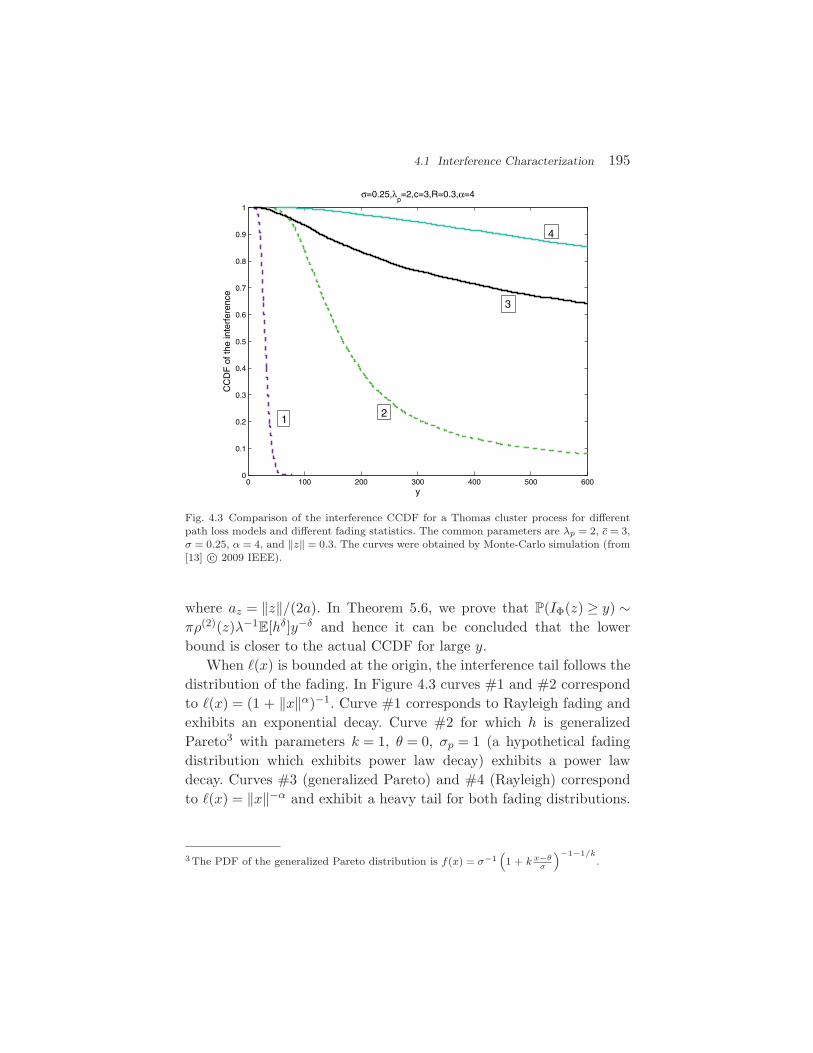
4.1 Interference Characterization 195
0 100 200 300 400 500 6000
0.1
0.2
0.3
0.4
0.5
0.6
0.7
0.8
0.9
1
y
CC
DF
of t
he in
terf
eren
ce
σ=0.25,λp=2,c=3,R=0.3,α=4
12
4
3
Fig. 4.3 Comparison of the interference CCDF for a Thomas cluster process for differentpath loss models and different fading statistics. The common parameters are λp = 2, c = 3,σ = 0.25, α = 4, and ‖z‖ = 0.3. The curves were obtained by Monte-Carlo simulation (from[13] c© 2009 IEEE).
where az = ‖z‖/(2a). In Theorem 5.6, we prove that P(IΦ(z) ≥ y) ∼πρ(2)(z)λ−1
E[hδ]y−δ and hence it can be concluded that the lowerbound is closer to the actual CCDF for large y.
When (x) is bounded at the origin, the interference tail follows thedistribution of the fading. In Figure 4.3 curves #1 and #2 correspondto (x) = (1 + ‖x‖α)−1. Curve #1 corresponds to Rayleigh fading andexhibits an exponential decay. Curve #2 for which h is generalizedPareto3 with parameters k = 1, θ = 0, σp = 1 (a hypothetical fadingdistribution which exhibits power law decay) exhibits a power lawdecay. Curves #3 (generalized Pareto) and #4 (Rayleigh) correspondto (x) = ‖x‖−α and exhibit a heavy tail for both fading distributions.
3 The PDF of the generalized Pareto distribution is f(x) = σ−1(1 + k x−θ
σ
)−1−1/k.

196 Interference in Poisson Cluster Networks
We can also use the conditional Laplace transform to obtain thenearest-neighbor distribution as N(r) = G[1b(o,r)c(x)]. All the reducedPalm moments of the PCP can be derived from the conditional PGFLobtained before.
4.2 Outage Analysis
The probability of success for the transmitter located at the origin andits receiver at z is
ps(θ) = P
( h(z)W + IΦ\o(z)
≥ θ | transmitter at the origin)
= P!o( h(z)W + IΦ(z)
≥ θ). (4.12)
For Rayleigh fading,
ps(θ) =∫ ∞
0e−sθ/(z)dP
!o(W + IΦ(z) ≤ s)
= L!oIΦ(z)(θ/(z))LW (θ/(z)). (4.13)
L!oIΦ(z) is the conditional Laplace transform of the interference and LW
denotes the Laplace transform of the noise. We now use the conditionalPGFL of PCP and (4.13) to evaluate the success probability.
Theorem 4.4 (Success probability). The probability of successfultransmission between the transmitter at the origin and the receiverlocated at z ∈ R
2, when W ≡ 0 (no noise), is
Ps(θ) = exp− λp
∫R2
[1 − exp(−cβ(z,y))
]dy
︸ ︷︷ ︸T1
×∫
R2exp(−cβ(z,y))fcl(y)dy︸ ︷︷ ︸
T2
, (4.14)
where
β(z,y) =∫
R2
(x − y − z)(z)θ + (x − y − z)
fcl(x)dx. (4.15)
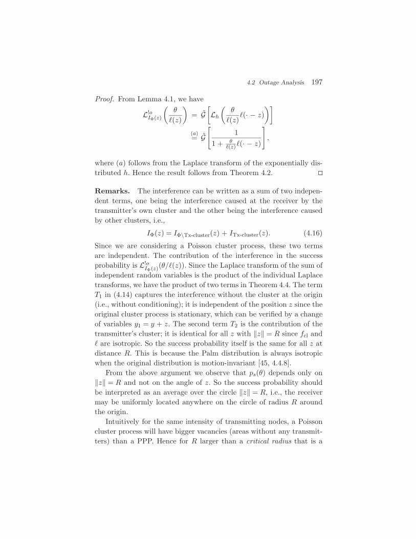
4.2 Outage Analysis 197
Proof. From Lemma 4.1, we have
L!oIΦ(z)
(θ
(z)
)= G
[Lh
(θ
(z)(· − z)
)](a)= G
[1
1 + θ(z)(· − z)
],
where (a) follows from the Laplace transform of the exponentially dis-tributed h. Hence the result follows from Theorem 4.2.
Remarks. The interference can be written as a sum of two indepen-dent terms, one being the interference caused at the receiver by thetransmitter’s own cluster and the other being the interference causedby other clusters, i.e.,
IΦ(z) = IΦ\Tx-cluster(z) + ITx-cluster(z). (4.16)
Since we are considering a Poisson cluster process, these two termsare independent. The contribution of the interference in the successprobability is L!o
IΦ(z)(θ/(z)). Since the Laplace transform of the sum ofindependent random variables is the product of the individual Laplacetransforms, we have the product of two terms in Theorem 4.4. The termT1 in (4.14) captures the interference without the cluster at the origin(i.e., without conditioning); it is independent of the position z since theoriginal cluster process is stationary, which can be verified by a changeof variables y1 = y + z. The second term T2 is the contribution of thetransmitter’s cluster; it is identical for all z with ‖z‖ = R since fcl and are isotropic. So the success probability itself is the same for all z atdistance R. This is because the Palm distribution is always isotropicwhen the original distribution is motion-invariant [45, 4.4.8].
From the above argument we observe that ps(θ) depends only on‖z‖ = R and not on the angle of z. So the success probability shouldbe interpreted as an average over the circle ‖z‖ = R, i.e., the receivermay be uniformly located anywhere on the circle of radius R aroundthe origin.
Intuitively for the same intensity of transmitting nodes, a Poissoncluster process will have bigger vacancies (areas without any transmit-ters) than a PPP. Hence for R larger than a critical radius that is a
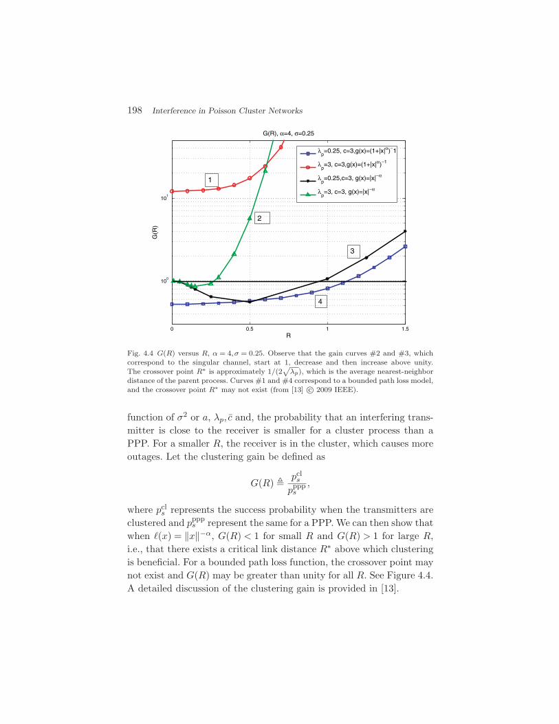
198 Interference in Poisson Cluster Networks
0 0.5 1 1.5
100
101
R
G(R
)
G(R), α=4, σ=0.25
λp=0.25, c=3,g(x)=(1+|x|α)−1
λp=3, c=3,g(x)=(1+|x|α)−1
λp=0.25,c=3, g(x)=|x|−α
λp=3, c=3, g(x)=|x|−α
1
2
3
4
Fig. 4.4 G(R) versus R, α = 4,σ = 0.25. Observe that the gain curves #2 and #3, whichcorrespond to the singular channel, start at 1, decrease and then increase above unity.The crossover point R∗ is approximately 1/(2
√λp), which is the average nearest-neighbor
distance of the parent process. Curves #1 and #4 correspond to a bounded path loss model,and the crossover point R∗ may not exist (from [13] c© 2009 IEEE).
function of σ2 or a, λp, c and, the probability that an interfering trans-mitter is close to the receiver is smaller for a cluster process than aPPP. For a smaller R, the receiver is in the cluster, which causes moreoutages. Let the clustering gain be defined as
G(R) pcls
pppps
,
where pcls represents the success probability when the transmitters are
clustered and pppps represent the same for a PPP. We can then show that
when (x) = ‖x‖−α, G(R) < 1 for small R and G(R) > 1 for large R,i.e., that there exists a critical link distance R∗ above which clusteringis beneficial. For a bounded path loss function, the crossover point maynot exist and G(R) may be greater than unity for all R. See Figure 4.4.A detailed discussion of the clustering gain is provided in [13].
5Interference in General Motion-Invariant
Networks
5.1 System Model
In this section, we consider transmitters distributed in a stationaryand isotropic fashion on the plane. Stationary and isotropic point pro-cesses are also called motion-invariant. Please refer to the appendixfor a mathematical description of such point processes. We give fourexamples:
Homogeneous Poisson point process: A PPP of constant density λ
is a stationary and isotropic point process and hence motion-invariant.Also any point process with finite number of points in the plane cannotbe stationary and hence cannot be motion-invariant.
Poisson cluster process: Poisson cluster processes, defined in theappendix and analyzed in Section 4, are motion-invariant.
Shifted lattice process: This point process Φ is the randomly translatedand rotated square lattice. More precisely,
Φ =√λZ
2ejβ + U,
where β is uniformly distributed in [0,2π] and U is uniformly dis-tributed in [0,
√λ].
199

200 Interference in General Motion-Invariant Networks
Hole-1 process: Consider two stationary PPPs Φs and Φp of intensitiesλs and λp with λp < λs. The lower intensity process Φp models theprimary users and Φs the secondary users in a cognitive network. Asecondary user x ∈ Φs with no primary user in a disk of radius a arounditself is allowed to transmit. More formally,
Φts = x ∈ Φs : b(x,a) ∩ Φp = ∅.
The average number of secondary transmitters in a set B is
EΦts(B) = E
∑x∈Φs∩B
∏y∈Φp
(1 − 1b(x,a)(y)
)(a)= E
∑x∈Φs∩B
E
∏y∈Φp
(1 − 1b(x,a)(y)
)(b)= E
∑x∈Φs∩B
exp(−λp
∫R2
1b(x,a)(y)dy)
(c)= λs exp(−λpπa2)|B|,
where (a) follows from the independence of the two point process, (b)follows from the PGFL of Φp, and (c) follows from the Campbell theo-rem applied to Φs. From the above, we observe that the density of Φt
s
is λs exp(−λpπa2).Every transmitter is assumed to transmit with unit power. The
intended transmitter is located at the origin and is a part of the trans-mit point process Φ. The interference observed at z ∈ R
2 is
IΦ(z) =∑
x∈Φ\ohx(x − z), (5.1)
where the fading process hx is iid with CDF Fh, PDF fh, and unit mean.In this section we provide the characterization of the (complementary)CDF of IΦ(z) given that there is a transmitting node at the origin. So allprobabilities are conditioned on the event that there is a transmittingnode at the origin, i.e., we are using Palm probabilities [8, 29, 45]. LetG[v] denote the conditional probability generating functional of thepoint process Φ, i.e.,
G[v] = E!o
[∏x∈Φ
v(x)
], (5.2)
5.2 Properties of the Interference 201
where v : R2→ [0,∞) is a well-behaved function [8].
In this section, we will also consider the effect of the path loss func-tion (x) on the distribution of the interference. We consider the fol-lowing path loss models:
(1) Singular model: (x) = ‖x‖−α, α > 2.(2) Non-singular (bounded) model: (x) = (1 + ‖x‖α)−1, α > 2.
We require α > 2 since we want∫b(o,1)c l(x) <∞, i.e., the path loss
model should be well-behaved except possibly at the origin. In the liter-ature [11], an exponential path loss model i.e., (x) = exp(−γ‖x‖)/‖x‖αis also used. But from the interference perspective, it is similar to thesingular path loss model. As before, we will use δ to denote 2/α.
5.2 Properties of the Interference
We first start by deriving the first and the second conditional momentsof the interference.
Lemma 5.1. The mean interference is
E!o[IΦ(z)] =
1λ
∫R2(x − z)ρ(2)(x)dx.
Proof.
E!o[IΦ(z)] = E
!o∑x∈Φ
hx(x − z)
(a)= E[h]λ
∫R2(x − z)K2(dx)
(b)=
1λ
∫R2(x − z)ρ(2)(x)dx.
(a) follows from the definition of the n-th factorial moment measure,see (A.10) and (b) from the definition of ρ(2)(x).
The average interference is finite for the non-singular path loss model.For (x) = ‖x‖−α, the average interference is finite if and only if ρ(2)(x)
202 Interference in General Motion-Invariant Networks
is zero in a small neighborhood of z. From the definition of ρ(2)(x) thisimplies that there should not be any interfering transmitter close tothe receiver located at z. For a PPP and PCP ρ(2)(z) = 0 for z > 0 andhence the average interference is infinite. For the shifted lattice process,ρ(2)(x) = 0 for ‖x‖ <
√λ and hence the average interference is finite for
z <√λ.
Lemma 5.2. The second moment of the interference is
E!o[I2
Φ(z)] =E[h2]λ
∫R22(x − z)ρ(2)(x)dx
+E[h]2
λ
∫R2
∫R2(x1 − z)(x2 − z)ρ(3)(x1,x2)dx1dx2.
Proof. We have
E!o[I2
Φ(z)]
= E!o[∑
x∈Φ
hx(x − z)]2
= E!o
[∑x∈Φ
h2x
2(x − z)]
+ E!o
=∑
x1,x2∈Φ
hx1hx2(x1 − z)(x2 − z)
(a)= E[h2]E!o
[∑x∈Φ
2(x − z)]
+ E[h]2E!o
=∑
x1,x2∈Φ
(x1 − z)(x2 − z)
,
where∑= indicates that the summation is to be taken over all pairs of
distinct points in Φ. (a) follows from the independence of the fading.For the first term,
E!o
[∑x∈Φ
2(x − z)]
(a)= λ
∫R22(x − z)K2(dx)
(b)=
1λ
∫R22(x − z)ρ(2)(x)dx.
5.3 Bounds on the Interference Distribution 203
Similarly, for the second term,
E!o
[ =∑x1,x2∈Φ
(x1 − z)(x2 − z)]
(c)= λ2
∫R2
∫R2(x1 − z)(x2 − z)K3(dx1 × dx2)
(d)=
1λ
∫R2
∫R2(x1 − z)(x2 − z)ρ(3)(x1,x2)dx1dx2.
(a), (b), (c), and (d) follow from the definition of the n-th order productdensity in the appendix.
When Φ is PPP, we have ρ(2)(x) = λ2 and ρ(3)(x) = λ3 and hence
E!o[I2
Φ(z)] = E[h2]λ∫
R22(x)dx + E[h]2λ2
(∫R2(x)dx
)2
,
in agreement with (3.52). We observe that the interference momentsand hence the distribution depend on the location z for a general pointprocess. The distribution of the IΦ(z) does not depend on the direc-tion of z because of the isotropy of the Palm distribution for motion-invariant processes.
5.3 Bounds on the Interference Distribution
In the previous sections, we have derived the Laplace transform of theinterference for the PPP and the PCP. Although in theory, the Laplacetransform provides the complete description of the interference, it ismore beneficial to know the CDF or the PDF of the interference explic-itly. In this section we provide bounds on the CCDF of the interferencewhen the transmitting nodes are homogeneously distributed on theplane.
The basic idea behind the proof is easy to understand when fading isabsent, (x) = ‖x‖−α and for a PPP. In this case the interference at theorigin is given by I =
∑x∈Φ (x). We can then divide the transmitting
set into two subsets, denoted as the near set and the far set. The near
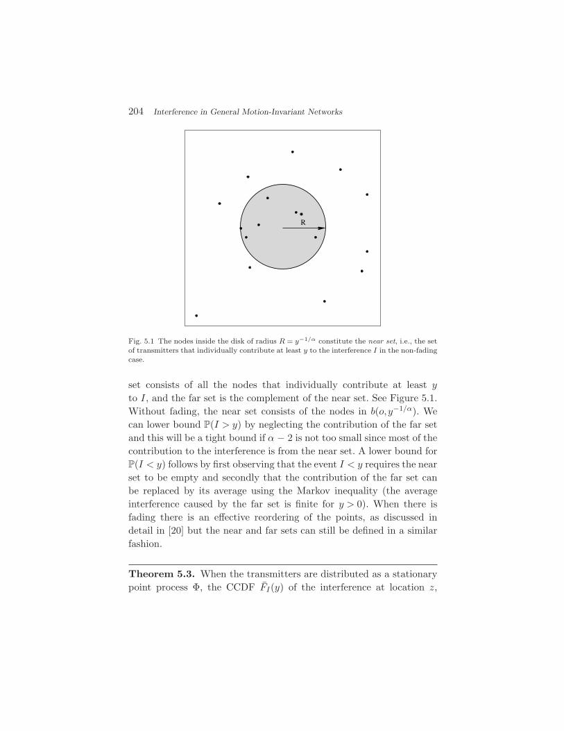
204 Interference in General Motion-Invariant Networks
R
Fig. 5.1 The nodes inside the disk of radius R = y−1/α constitute the near set, i.e., the setof transmitters that individually contribute at least y to the interference I in the non-fadingcase.
set consists of all the nodes that individually contribute at least yto I, and the far set is the complement of the near set. See Figure 5.1.Without fading, the near set consists of the nodes in b(o,y−1/α). Wecan lower bound P(I > y) by neglecting the contribution of the far setand this will be a tight bound if α − 2 is not too small since most of thecontribution to the interference is from the near set. A lower bound forP(I < y) follows by first observing that the event I < y requires the nearset to be empty and secondly that the contribution of the far set canbe replaced by its average using the Markov inequality (the averageinterference caused by the far set is finite for y > 0). When there isfading there is an effective reordering of the points, as discussed indetail in [20] but the near and far sets can still be defined in a similarfashion.
Theorem 5.3. When the transmitters are distributed as a stationarypoint process Φ, the CCDF FI(y) of the interference at location z,
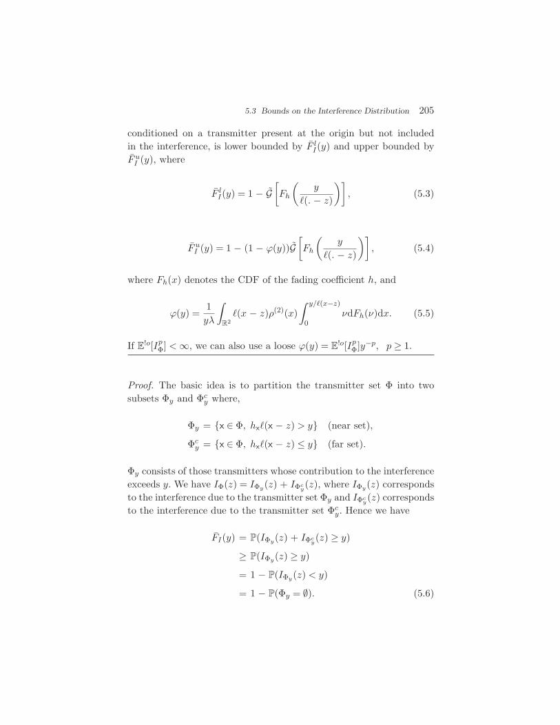
5.3 Bounds on the Interference Distribution 205
conditioned on a transmitter present at the origin but not includedin the interference, is lower bounded by F lI(y) and upper bounded byF uI (y), where
F lI(y) = 1 − G[Fh
(y
(. − z)
)], (5.3)
F uI (y) = 1 − (1 − ϕ(y))G[Fh
(y
(. − z)
)], (5.4)
where Fh(x) denotes the CDF of the fading coefficient h, and
ϕ(y) =1yλ
∫R2(x − z)ρ(2)(x)
∫ y/(x−z)
0νdFh(ν)dx. (5.5)
If E!o[IpΦ] <∞, we can also use a loose ϕ(y) = E
!o[IpΦ]y−p, p ≥ 1.
Proof. The basic idea is to partition the transmitter set Φ into twosubsets Φy and Φc
y where,
Φy = x ∈ Φ, hx(x − z) > y (near set),
Φcy = x ∈ Φ, hx(x − z) ≤ y (far set).
Φy consists of those transmitters whose contribution to the interferenceexceeds y. We have IΦ(z) = IΦy(z) + IΦc
y(z), where IΦy(z) corresponds
to the interference due to the transmitter set Φy and IΦcy(z) corresponds
to the interference due to the transmitter set Φcy. Hence we have
FI(y) = P(IΦy(z) + IΦcy(z) ≥ y)
≥ P(IΦy(z) ≥ y)
= 1 − P(IΦy(z) < y)
= 1 − P(Φy = ∅). (5.6)

206 Interference in General Motion-Invariant Networks
We can find the probability P(Φy = ∅) that Φy is empty using the con-ditional Laplace functional as follows:
P(Φy = ∅) = E!o∏x∈Φ
1hx(x−z)≤y
(a)= E
!o∏x∈Φ
Eh
(1hx(x−z)≤y
)= E
!o∏x∈Φ
Fh
(y
(x − z)
)
= G[Fh
(y
(· − z)
)], (5.7)
where (a) follows from the independence of hx. To obtain the upperbound,
FI(y) = P(IΦ > y | IΦy > y)F lI(y) + P(IΦ > y | IΦy ≤ y)(1 − F lI(y))(a)= 1 − G
[Fh
(y
(· − z)
)]
+P(IΦ > y | IΦy ≤ y) G[Fh
(y
(· − z)
)]
= 1 − (1 − P(IΦ > y | IΦy ≤ y)) G[Fh
(y
(· − z)
)], (5.8)
where (a) follows from the lower bound we have established. To boundP(IΦ > y | IΦy ≤ y) we use the Markov inequality. We have
P(IΦ > y | IΦy ≤ y) = P(IΦ > y | Φy = ∅)(a)≤ E
!o (IΦ | Φy = ∅)y
=1y
E!o∑x∈Φ
hx(x − z)1hx(x−z)≤y
=1y
E!o∑x∈Φ
(x − z)∫ y/(x−z)
0νdFh(ν)
(b)=
1yλ
∫R2(x − z)
∫ y/(x−z)
0νdFh(ν)ρ(2)(x)dx,

5.3 Bounds on the Interference Distribution 207
where (a) follows from the Markov inequality, and (b) follows from aprocedure similar to the calculation of the mean interference in theprevious section.
Since isotropy is not used in the proof, Theorem 5.3 holds for sta-tionary point processes, not just motion-invariant ones.
When Φ is a PPP, we have G[v] = exp(−λ∫
1 − v(x)dx) (A.3). ForRayleigh fading and (x) = ‖x‖−α, the lower bound is
F lI(y) = 1 − exp(−πλy−δΓ(1 + δ)),
and the upper bound is
F uI (y) = 1 −(
1 − 2πλΓ(1 + δ)α − 2
y−δ)
exp(−πλy−δΓ(1 + δ)).
From Figure 5.2, we observe that the lower bound is closer to the actualCCDF than the upper bound. In the above derivation, the upper boundmay be loose because a simple Markov inequality is used to boundP(IΦ > y | IΦy ≤ y), and a better bound may be obtained by using theChernoff bound. The upper bound diverges as α ↓ 2 since the averageinterference contribution from the far set diverges. From the upper andlower bounds we can (once again) infer that the interference in a PPPnetwork is heavy-tailed with parameter δ for the singular path lossmodel.
In the next lemma we prove that the upper and lower bounds areasymptotically tight when (x) = ‖x‖−α. We will use g1(x) ∼ g2(x) todenote limx→∞ g1(x)/g2(x) = 1.
Lemma 5.4. When (x) = ‖x‖−α, α > 2, z ∈ R2 and ρ(2)(z) continu-
ous in a small neighborhood of z,
ϕ(y)
∼ πρ(2)(z)E[hδ ]
λ(δ−1−1) y−δ ρ(2)(z) = 0
= o(y−δ) ρ(2)(z) = 0.

208 Interference in General Motion-Invariant Networks
0 10 20 30 40 50
0.4
0.5
0.6
0.7
0.8
0.9
1
y
CC
DF
of
I Φ
α=4, λ=1
Lower bound
Actual
Upper bound
Fig. 5.2 The CCDF of the interference is plotted when Φ is a PPP and (x) = ‖x‖−4. In thiscase the interference is a Levy-stable distribution (3.20).
Proof. When (x) = ‖x‖−α,α > 2, we have
ϕ(y) =1yλ
∫R2‖x − z‖−αρ(2)(x)
∫ ‖x−z‖α
0νdFh(ν)dx
(a)=
1yλ
∫ ∞
0ν
∫R2‖x‖−α1‖x‖α>νy−1ρ(2)(x + z)dxdFh(ν)
(b)=
y−δ
λ
∫ ∞
0ν
∫R2‖x‖−α1‖x‖α>νρ
(2)(
x
y1/α + z
)dxdFh(ν),
where (a) follows from the substitution x→ x + z and interchangingthe integrals. (b) follows by the substitution y1/αx→ x. So by the dom-inated convergence theorem, we have for ρ(2)(z) = 0
limy→0
ϕ(y)y−δ =
ρ(2)(z)λ
∫ ∞
0ν
∫R2‖x‖−α1‖x‖α>νdxdFh(ν)
=2πρ(2)(z)E[h2/α]
λ(α − 2).
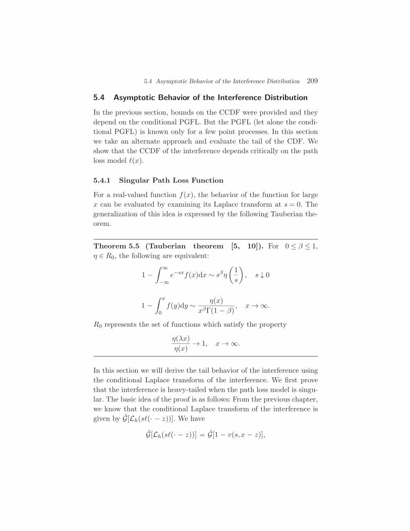
5.4 Asymptotic Behavior of the Interference Distribution 209
5.4 Asymptotic Behavior of the Interference Distribution
In the previous section, bounds on the CCDF were provided and theydepend on the conditional PGFL. But the PGFL (let alone the condi-tional PGFL) is known only for a few point processes. In this sectionwe take an alternate approach and evaluate the tail of the CDF. Weshow that the CCDF of the interference depends critically on the pathloss model (x).
5.4.1 Singular Path Loss Function
For a real-valued function f(x), the behavior of the function for largex can be evaluated by examining its Laplace transform at s = 0. Thegeneralization of this idea is expressed by the following Tauberian the-orem.
Theorem 5.5 (Tauberian theorem [5, 10]). For 0 ≤ β ≤ 1,η ∈ R0, the following are equivalent:
1 −∫ ∞
−∞e−sxf(x)dx ∼ sβη
(1s
), s ↓ 0
1 −∫ x
0f(y)dy ∼ η(x)
xβΓ(1 − β), x→∞.
R0 represents the set of functions which satisfy the property
η(λx)η(x)
→ 1, x→∞.
In this section we will derive the tail behavior of the interference usingthe conditional Laplace transform of the interference. We first provethat the interference is heavy-tailed when the path loss model is singu-lar. The basic idea of the proof is as follows: From the previous chapter,we know that the conditional Laplace transform of the interference isgiven by G[Lh(s(· − z))]. We have
G[Lh(s(· − z))] = G[1 − v(s,x − z)],
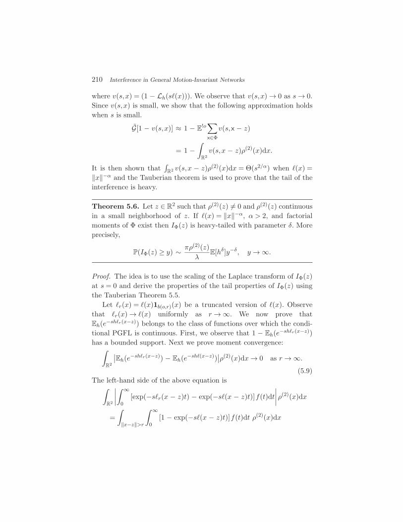
210 Interference in General Motion-Invariant Networks
where v(s,x) = (1 − Lh(s(x))). We observe that v(s,x)→ 0 as s→ 0.Since v(s,x) is small, we show that the following approximation holdswhen s is small.
G[1 − v(s,x)] ≈ 1 − E!o∑x∈Φ
v(s,x − z)
= 1 −∫
R2v(s,x − z)ρ(2)(x)dx.
It is then shown that∫
R2 v(s,x − z)ρ(2)(x)dx = Θ(s2/α) when (x) =‖x‖−α and the Tauberian theorem is used to prove that the tail of theinterference is heavy.
Theorem 5.6. Let z ∈ R2 such that ρ(2)(z) = 0 and ρ(2)(z) continuous
in a small neighborhood of z. If (x) = ‖x‖−α, α > 2, and factorialmoments of Φ exist then IΦ(z) is heavy-tailed with parameter δ. Moreprecisely,
P(IΦ(z) ≥ y) ∼ πρ(2)(z)λ
E[hδ]y−δ, y→∞.
Proof. The idea is to use the scaling of the Laplace transform of IΦ(z)at s = 0 and derive the properties of the tail properties of IΦ(z) usingthe Tauberian Theorem 5.5.
Let r(x) = (x)1b(o,r)(x) be a truncated version of (x). Observethat r(x)→ (x) uniformly as r→∞. We now prove thatEh(e−shr(x−z)) belongs to the class of functions over which the condi-tional PGFL is continuous. First, we observe that 1 − Eh(e−shr(x−z))has a bounded support. Next we prove moment convergence:∫
R2
∣∣Eh(e−shr(x−z)) − Eh(e−sh(x−z))∣∣ρ(2)(x)dx→ 0 as r→∞.
(5.9)The left-hand side of the above equation is∫
R2
∣∣∣∣∫ ∞
0[exp(−sr(x − z)t) − exp(−s(x − z)t)]f(t)dt
∣∣∣∣ρ(2)(x)dx
=∫
‖x−z‖>r
∫ ∞
0[1 − exp(−s(x − z)t)]f(t)dt ρ(2)(x)dx
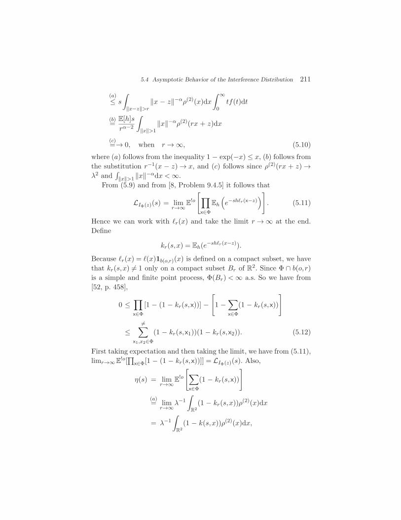
5.4 Asymptotic Behavior of the Interference Distribution 211
(a)≤ s
∫‖x−z‖>r
‖x − z‖−αρ(2)(x)dx∫ ∞
0tf(t)dt
(b)=
E[h]srα−2
∫‖x‖>1
‖x‖−αρ(2)(rx + z)dx
(c)=→ 0, when r→∞, (5.10)
where (a) follows from the inequality 1 − exp(−x) ≤ x, (b) follows fromthe substitution r−1(x − z)→ x, and (c) follows since ρ(2)(rx + z)→λ2 and
∫‖x‖>1 ‖x‖−αdx <∞.
From (5.9) and from [8, Problem 9.4.5] it follows that
LIΦ(z)(s) = limr→∞
E!o
[∏x∈Φ
Eh
(e−shr(x−z)
)]. (5.11)
Hence we can work with r(x) and take the limit r→∞ at the end.Define
kr(s,x) = Eh(e−shr(x−z)).
Because r(x) = (x)1b(o,r)(x) is defined on a compact subset, we havethat kr(s,x) = 1 only on a compact subset Br of R
2. Since Φ ∩ b(o,r)is a simple and finite point process, Φ(Br) <∞ a.s. So we have from[52, p. 458],
0 ≤∏x∈Φ
[1 − (1 − kr(s,x))] −[1 −
∑x∈Φ
(1 − kr(s,x))]
≤=∑
x1,x2∈Φ
(1 − kr(s,x1))(1 − kr(s,x2)). (5.12)
First taking expectation and then taking the limit, we have from (5.11),limr→∞ E
!o[∏
x∈Φ[1 − (1 − kr(s,x))]] = LIΦ(z)(s). Also,
η(s) = limr→∞
E!o
[∑x∈Φ
(1 − kr(s,x))]
(a)= lim
r→∞λ−1
∫R2
(1 − kr(s,x))ρ(2)(x)dx
= λ−1∫
R2(1 − k(s,x))ρ(2)(x)dx,
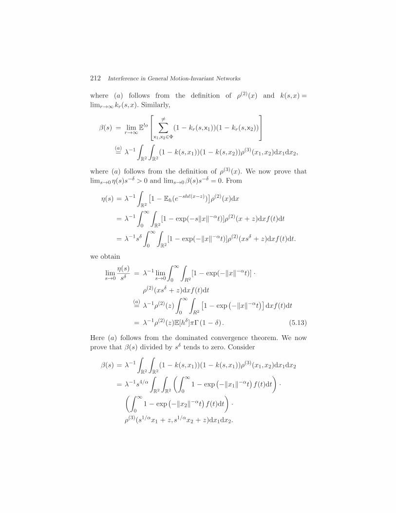
212 Interference in General Motion-Invariant Networks
where (a) follows from the definition of ρ(2)(x) and k(s,x) =limr→∞kr(s,x). Similarly,
β(s) = limr→∞
E!o
=∑
x1,x2∈Φ
(1 − kr(s,x1))(1 − kr(s,x2))
(a)= λ−1
∫R2
∫R2
(1 − k(s,x1))(1 − k(s,x2))ρ(3)(x1,x2)dx1dx2,
where (a) follows from the definition of ρ(3)(x). We now prove thatlims→0 η(s)s−δ > 0 and lims→0β(s)s−δ = 0. From
η(s) = λ−1∫
R2
[1 − Eh(e−sh(x−z))
]ρ(2)(x)dx
= λ−1∫ ∞
0
∫R2
[1 − exp(−s‖x‖−αt)]ρ(2)(x + z)dxf(t)dt
= λ−1sδ∫ ∞
0
∫R2
[1 − exp(−‖x‖−αt)]ρ(2)(xsδ + z)dxf(t)dt.
we obtain
lims→0
η(s)sδ
= λ−1 lims→0
∫ ∞
0
∫R2
[1 − exp(−‖x‖−αt)] ·
ρ(2)(xsδ + z)dxf(t)dt
(a)= λ−1ρ(2)(z)
∫ ∞
0
∫R2
[1 − exp
(−‖x‖−αt
)]dxf(t)dt
= λ−1ρ(2)(z)E[hδ]πΓ(1 − δ) . (5.13)
Here (a) follows from the dominated convergence theorem. We nowprove that β(s) divided by sδ tends to zero. Consider
β(s) = λ−1∫
R2
∫R2
(1 − k(s,x1))(1 − k(s,x1))ρ(3)(x1,x2)dx1dx2
= λ−1s4/α∫
R2
∫R2
(∫ ∞
01 − exp
(−‖x1‖−αt
)f(t)dt
)·(∫ ∞
01 − exp
(−‖x2‖−αt
)f(t)dt
)·
ρ(3)(s1/αx1 + z,s1/αx2 + z)dx1dx2.
5.4 Asymptotic Behavior of the Interference Distribution 213
The integral is finite because ρ(3)(x,y) < log(‖x‖) log(‖y‖) for large |x|and |y|. Hence
lims→0
β(s)sδ
= 0. (5.14)
From (5.12), we have
0 ≤ LIΦ(z)(s) − (1 − η(s)) ≤ β(s).
Dividing both sides by sδ, taking the limit s→ 0 and using (5.13) and(5.14),
lims→0
1 − LIΦ(z)(s)sδ
=πρ(2)(z)
λE[hδ]Γ(1 − δ) .
So we have
1 − LIΦ(z)(s) ∼πρ(2)(z)
λE[hδ]Γ(1 − δ)sδ.
So using the Tauberian Theorem 5.5,
P(IΦ(z) ≥ y) ∼ πρ(2)(z)λ
E[hδ]y−δ.
From the above theorem we observe that interference at z is alwaysheavy-tailed with parameter δ when the path loss model is singular andρ(2)(z) = 0. This is because the receiver is not a part of the process anda transmitter can be arbitrarily close to it, which causes the interferenceto be very large with finite probability. This is consistent with (3.25).
5.4.2 Non-singular Path Loss Function
We now investigate the interference distribution when the path loss isnon-singular or bounded. In this case, the existence of an interferer closeto a receiver will not alter the magnitude of the interference drastically.Instead the fading becomes an important factor, and the distributiontail depends mainly on the tail of the fading. We will use the followingtheorem that connects the convergence region of the Laplace transformof a random variable and the decay of its CCDF.
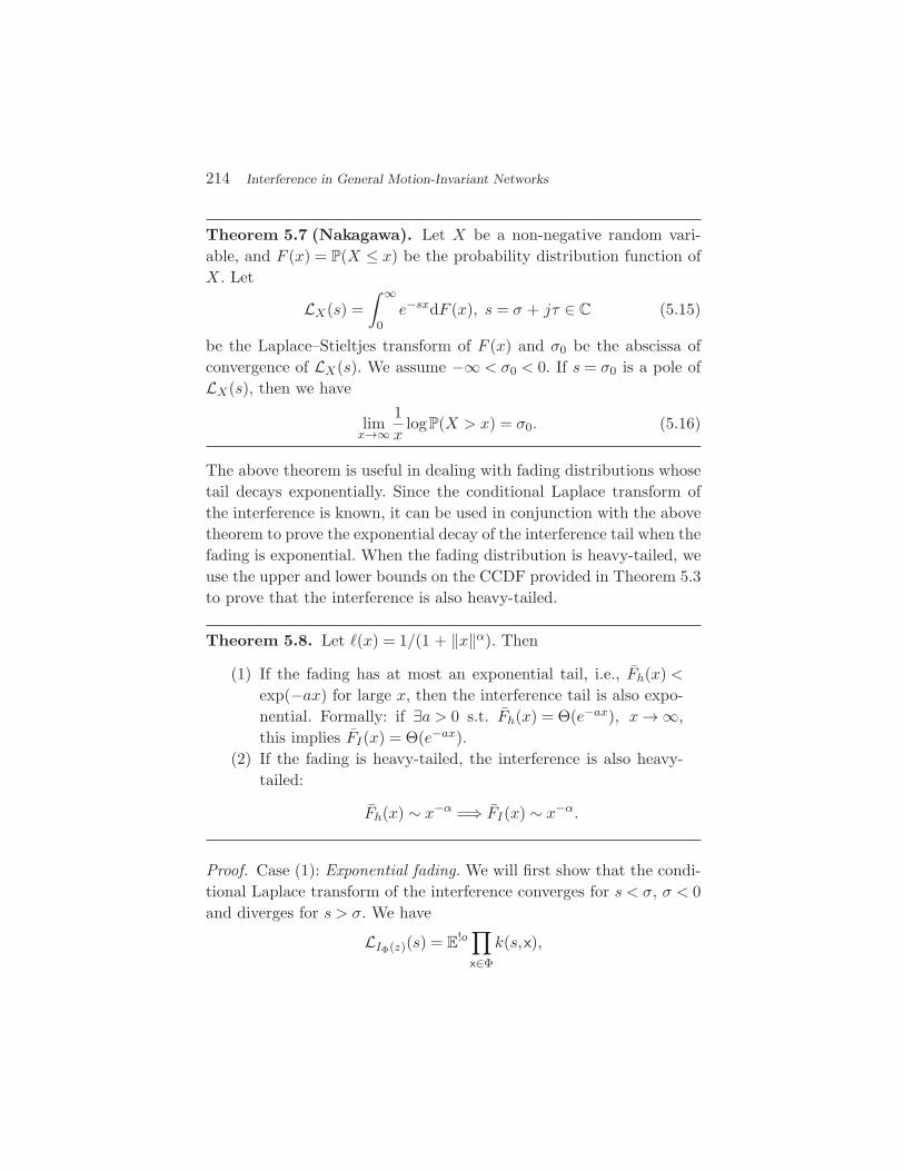
214 Interference in General Motion-Invariant Networks
Theorem 5.7 (Nakagawa). Let X be a non-negative random vari-able, and F (x) = P(X ≤ x) be the probability distribution function ofX. Let
LX(s) =∫ ∞
0e−sxdF (x), s = σ + jτ ∈ C (5.15)
be the Laplace–Stieltjes transform of F (x) and σ0 be the abscissa ofconvergence of LX(s). We assume −∞ < σ0 < 0. If s = σ0 is a pole ofLX(s), then we have
limx→∞
1x
logP(X > x) = σ0. (5.16)
The above theorem is useful in dealing with fading distributions whosetail decays exponentially. Since the conditional Laplace transform ofthe interference is known, it can be used in conjunction with the abovetheorem to prove the exponential decay of the interference tail when thefading is exponential. When the fading distribution is heavy-tailed, weuse the upper and lower bounds on the CCDF provided in Theorem 5.3to prove that the interference is also heavy-tailed.
Theorem 5.8. Let (x) = 1/(1 + ‖x‖α). Then
(1) If the fading has at most an exponential tail, i.e., Fh(x) <exp(−ax) for large x, then the interference tail is also expo-nential. Formally: if ∃a > 0 s.t. Fh(x) = Θ(e−ax), x→∞,this implies FI(x) = Θ(e−ax).
(2) If the fading is heavy-tailed, the interference is also heavy-tailed:
Fh(x) ∼ x−α =⇒ FI(x) ∼ x−α.
Proof. Case (1): Exponential fading. We will first show that the condi-tional Laplace transform of the interference converges for s < σ, σ < 0and diverges for s > σ. We have
LIΦ(z)(s) = E!o∏x∈Φ
k(s,x),
5.4 Asymptotic Behavior of the Interference Distribution 215
where k(s,x) = Lh(s(x − z)). From the above equation we observethat LIΦ(z)(s) is finite if and only if
η(s) = E!o∑x∈Φ
| logk(s,x)| <∞.
We now show that the abscissa of convergence σ of LIΦ(z)(s) is strictlyless than zero, i.e., η(s) <∞ for some s < 0.
Let β(s,x,h) = exp( −sh
(1+‖x−z‖α)
). We have
η(s) = E!o∑x∈Φ
| logk(s,x)|
=∫
R2|log(Eh[β(s,x,h)])|ρ(2)(x)dx.
When s > 0, it is trivial to see that η(s) <∞. The rest of the proof canbe better understood by considering s < 0. Since Fh(x) ∼ exp(−ax),x→∞, it can be assumed without any loss of generality that the fadingPDF is f(x) = aexp(−ax), x > R, for some large R. We have
k(s,x) =∫ R
0β(s,x, t)dF (t)
+a∫ ∞
Rexp
(−t
[a +
s
(1 + ‖x − z‖α)
])dt. (5.17)
The first term is always finite. Considering the second term, we observethat the term in the exponent will be positive for all x when s > −a.Hence the integral converges when s > −a and k(s,x) is well-defined(especially in the neighborhood of z).1
Also observe that k(s,x) > 1 for s ∈ (−a,0). Let b ∈ (−a,0). We nowprove that η(b) <∞. Since k(b,x) > 1, we have log(k(b,x)) ≤ k(b,x) −1. Hence
η(s) ≤∫
R2[k(b,x) − 1]ρ(2)(x)dx
=∫b(o,κ)
[k(b,x) − 1]ρ(2)(x)dx +∫b(o,κ)c
[k(b,x) − 1]ρ(2)(x)dx
1 Observe the importance of 1 in the denominator of the second term. Without it ∀s < 0,k(s,x) would be undefined in an open neighborhood of z.
216 Interference in General Motion-Invariant Networks
for κ ∈ (0,∞). Since b > −a, k(b,x) is a well-behaved function, i.e.,bounded and smooth, and hence the first term in the above equationis bounded for any κ <∞. So if we prove that the second term isfinite, then η(b) <∞. For large ‖x‖ we have ρ(2)(x)→ λ2. We chooseκ such that for all ‖x‖ > κ , ρ(2)(x) is very close to λ2. Hence ρ(2)(x)is essentially a constant and proving∫
b(o,κ)c
(k(b,x) − 1)dx <∞
will be sufficient. We have∫b(o,κ)c
(k(b,x) − 1)dx =∫b(o,κ)c
∫ R
0[β(−|b|,x, t) − 1]f(t)dtdx︸ ︷︷ ︸
A
+∫b(o,κ)c
∫ ∞
R[β(−|b|,x, t) − 1]f(t)dtdx︸ ︷︷ ︸
B
.
Considering the first term A, we can increase κ such that
β(−|b|,x, t) = exp(
|b|t(1 + ‖x − z‖α)
)≈ 1 +
|b|t(1 + ‖x − z‖α)
. (5.18)
This can be done since t < R. Hence we have
A =∫b(o,κ)c
∫ R
0
|b|t(1 + ‖x − z‖α)
f(t)dtdx <∞.
Considering the second integral B, substituting for the fading PDF andafter some algebraic manipulation, we get
B = e−aR∫b(o,κ)c
a(1 + ‖x − z‖α)(β(−|b|,x,R) − 1)a(1 + ‖x − z‖α) − |b| dx
+e−aR∫b(o,κ)c
|b|a(1 + ‖x − z‖α) − |b|dx.
Since κ is large, using the approximation (5.18), it follows that B <∞.So we have shown that η(b) <∞ for all b ∈ (−a,∞). We also observethat η(s) =∞ for s < −a. So the abscissa is equal to −a < 0. From[36, Theorem 3], it then follows that the tail falls exponentially withparameter a.
5.4 Asymptotic Behavior of the Interference Distribution 217
Case (2): Fh ∼ h−a is a heavy-tailed distribution. In this casek(s,x) =∞ for all s < 0, and hence [36, Theorem 3] cannot be applied.We will use Theorem 5.3 that provides upper and lower bounds for theCCDF of the interference. We first evaluate G
[Fh( y(.−z)
)]for large y:
G[Fh
(y
(. − z)
)]= G [1 − [1 − Fh (y(1 + ‖x − z‖α))]]
(a)∼ G(1 − [y(1 + ‖x − z‖α)]−a
)(b)∼ 1 − y−aλ−1
∫R2
[(1 + ‖x − z‖α)]−a ρ(2)(x)dx,
where (a) follows by the continuity of G and the fact that y is large.(b) follows from an argument similar to Theorem 5.6. We also havefrom Theorem 5.3, that ϕ(y) = y−a
E!o[IΦ(z)a]. Here E
!o[IΦ(z)a] <∞because of the bounded nature of (x) and its sufficiently fast decayingtail. So from the upper bound in Theorem 5.3, we have
P(IΦ(z) > y)
< y−a[λ−1
∫R2
[(1 + ‖x − z‖α)]−α ρ(2)(x)dx + E!o[IΦ(z)a]
],
and from the lower bound
P(IΦ(z) > y) > y−aλ−1∫
R2[(1 + ‖x − z‖α)]−α ρ(2)(x)dx.
So the tail decays like y−a.
We now show that the distribution of interference decays exponentiallyfast at the origin. The basic idea is that there is some contribution fromsome point of the process, however, small it is.
Theorem 5.9. The CDF of the interference decays faster than anypolynomial at the origin, i.e., ∀n ∈ N,
P(IΦ(z) < y) = o(yn), y→ 0.

218 Interference in General Motion-Invariant Networks
Proof. Find a such that Fh(x) = o(xa). Choose k ∈ N such that k >n/a. From Theorem 5.3, we have
P(IΦ(z) < y) < G(Fh
(y
(. − z)
))
= E!o
[∏x∈Φ
Fh
(y
(x − z)
)| Φ has at least k points
].
Multiply both sides by y−n and take the limit y→ 0. On the right-handside, the limit can be moved inside the expectation by the dominatedconvergence theorem. Since there are at least k points almost surely onthe plane (because Φ is stationary), we have that the limit on the rightgoes to zero by our choice of k.
5.5 Examples and Simulation Results
In this section we give examples of the interference for different pointprocesses and fading distributions and give approximations for the dis-tribution.
5.5.1 Examples
We concentrate on three different point processes: the PPP, the Thomascluster process, and the shifted lattice process.
Poisson point processes. (1) Singular path loss model: (x) =‖x‖−αFrom Section 3, the Laplace transform of the interference is LIΦ(s) =exp(−λπsδE[hδ]Γ(1 − δ)). The Laplace transform is independent of z,hence the distribution is independent of the location z. Also LIΦ(s) isthe Laplace transform of a stable random variable with parameter δand hence heavy-tailed.
(2) Bounded path loss model: (x) = (1 + ‖x‖α)−1
We first consider the case of exponential fading, i.e., fh(x) =µexp(−µx). In this case,
LIΦ(s) = exp(−λπ πδ
sin(πδ)s
(µ + s)1−δ
).
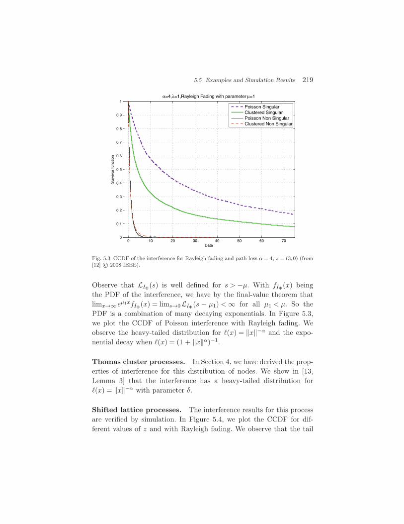
5.5 Examples and Simulation Results 219
0 10 20 30 40 50 60 700
0.1
0.2
0.3
0.4
0.5
0.6
0.7
0.8
0.9
1
Data
Sur
vivo
r fu
nctio
n
α=4,λ=1,Rayleigh Fading with parameter µ=1
Poisson SingularClustered SingularPoisson Non SingularClustered Non Singular
Fig. 5.3 CCDF of the interference for Rayleigh fading and path loss α = 4, z = (3,0) (from[12] c© 2008 IEEE).
Observe that LIΦ(s) is well defined for s > −µ. With fIΦ(x) beingthe PDF of the interference, we have by the final-value theorem thatlimx→∞ eµ1xfIΦ(x) = lims→0LIΦ(s − µ1) <∞ for all µ1 < µ. So thePDF is a combination of many decaying exponentials. In Figure 5.3,we plot the CCDF of Poisson interference with Rayleigh fading. Weobserve the heavy-tailed distribution for (x) = ‖x‖−α and the expo-nential decay when (x) = (1 + ‖x‖α)−1.
Thomas cluster processes. In Section 4, we have derived the prop-erties of interference for this distribution of nodes. We show in [13,Lemma 3] that the interference has a heavy-tailed distribution for(x) = ‖x‖−α with parameter δ.
Shifted lattice processes. The interference results for this processare verified by simulation. In Figure 5.4, we plot the CCDF for dif-ferent values of z and with Rayleigh fading. We observe that the tail
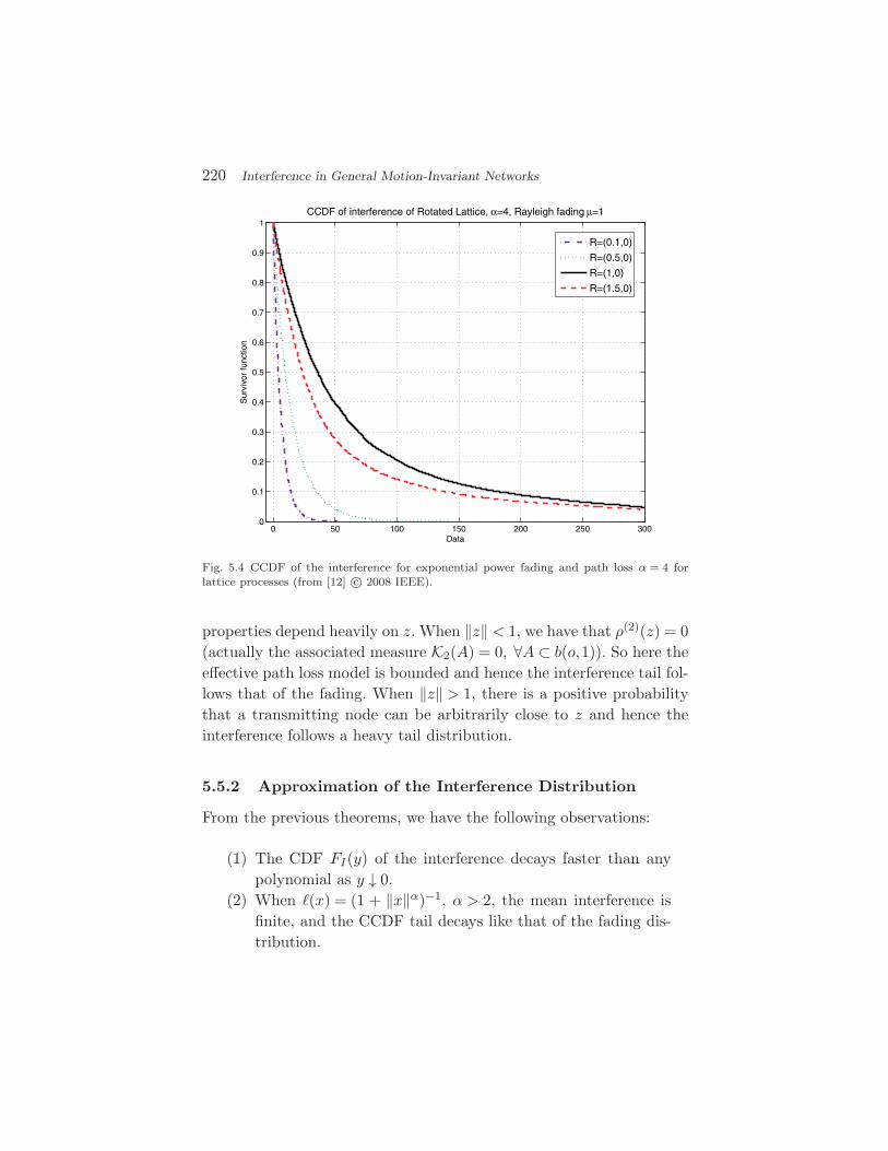
220 Interference in General Motion-Invariant Networks
0 50 100 150 200 250 3000
0.1
0.2
0.3
0.4
0.5
0.6
0.7
0.8
0.9
1
Data
Sur
vivo
r fu
nctio
n
CCDF of interference of Rotated Lattice, α=4, Rayleigh fading µ=1
R=(0.1,0)
R=(0.5,0)
R=(1,0)
R=(1.5,0)
Fig. 5.4 CCDF of the interference for exponential power fading and path loss α = 4 forlattice processes (from [12] c© 2008 IEEE).
properties depend heavily on z. When ‖z‖ < 1, we have that ρ(2)(z) = 0(actually the associated measure K2(A) = 0, ∀A ⊂ b(o,1)). So here theeffective path loss model is bounded and hence the interference tail fol-lows that of the fading. When ‖z‖ > 1, there is a positive probabilitythat a transmitting node can be arbitrarily close to z and hence theinterference follows a heavy tail distribution.
5.5.2 Approximation of the Interference Distribution
From the previous theorems, we have the following observations:
(1) The CDF FI(y) of the interference decays faster than anypolynomial as y ↓ 0.
(2) When (x) = (1 + ‖x‖α)−1, α > 2, the mean interference isfinite, and the CCDF tail decays like that of the fading dis-tribution.

5.5 Examples and Simulation Results 221
(3) When (x) = ‖x‖−α, the mean diverges, and the CDF has aheavy tail.
Observation 1 eliminates the use of Gaussian distribution to model theinterference except when the mean µ = E[IΦ] is very large (but finite),so that exp(−µ2/2σ2) is small. We choose three probability distribu-tions which have the desired properties. The gamma distribution, theinverse Gaussian distribution, and the inverse gamma distribution.
(1) Gamma distribution: f(x) = xk−1 exp(−x/a)/Γ(k)ak. Mean:ka, variance: ka2.
(2) Inverse Gaussian distribution:
f(x) =[ ν
2πx3
]1/2exp
(−κ(x − ν)
2
2ν2x
)
Mean: ν, variance: ν3/κ.
2 4 6 8 10 12 14 16 180
0.05
0.1
0.15
0.2
Data
Den
sity
PDF of Interference α =4
Interference Monte–Carlo simulationNonsingular Exponential fading
Inverse Gaussian,ν=4.9,κ=20.8
Gamma, k=5.1, θ=0.96
Normal
Inverse Gamma a=3, β =9.8
Fig. 5.5 Empirical PDF of the interference and the corresponding fits for (x) = (1 +‖x‖4)−1 and Rayleigh fading (mean 1) (from [12] c© 2008 IEEE).
222 Interference in General Motion-Invariant Networks
(3) Inverse gamma distribution:
f(x) = βax−a−1 exp(−β/x)Γ(a)−1
Mean: β/(a − 1), variance: β2/((a − 1)2(a − 2)).
In the inverse Gaussian distribution, the mean and variance can bechosen independently of each other. The gamma distribution only hasa (k − 1)-th order of decay at the origin and has an exponential tail.On the other hand, the inverse Gaussian distribution has an exponen-tial decay at origin and a slightly super-exponential tail. In Figure 5.5,we have plotted2 the PDF of the interference using Monte-Carlo sim-ulation when the underlying node distribution is PPP and the fadingis Rayleigh with a non-singular path loss model. We observe that thenormal fit performs the worst. Both the gamma and inverse Gaussiangive us a good fit. The inverse gamma PDF is a bad fit since it has afourth-order decaying tail, while the fading is exponentially decaying.In finite networks, where the number of nodes is finite and fixed andthe nodes are distributed on a bounded subset of the Euclidean plane,the interference does not decay superpolynomially fast at the origin,but only goes to zero like yna where n is the number of transmittersand a the decay of the fading CDF at the origin.
2 We have used a square of size 40 × 40 for simulation and averaged over 200,000 instances.
6Conclusions
The cumulated interference power in wireless networks can be sharplycharacterized in certain cases. Most notably, in the case of a homo-geneous Poisson network, at least the Laplace transform of the inter-ference can be derived. For the power law path loss with singularityat the origin, the interference follows a stable distribution if the pathloss exponent α exceeds the number of network dimensions d, other-wise the interference is infinite a.s. This result holds irrespective of thefading statistics and the number of network dimensions, and it impliesthat the mean interference does not exist. The dimensionality of thenetwork and the path loss exponent enter the Laplace transform onlythrough their ratio δ = d/α, which is exactly the characteristic expo-nent of the stable distribution, and the fading process only through itsδ-th moment. The Laplace transform, evaluated at the SIR thresholdθ, is the success probability of a transmission where the desired sig-nal power is exponentially distributed, e.g., due to Rayleigh fading. Soin this case, the SIR distribution is known for all parameters α andd, whereas the PDF of the interference only exists when the ratio isδ = 1/2.
223
224 Conclusions
ALOHA is the only MAC scheme that preserves the Poisson dis-tribution, since it performs independent thinning from the process ofall nodes to the process of transmitting nodes. Accordingly, ALOHAhas naturally received considerable attention in the literature, see, e.g.,[2, 3, 51]. In addition to its analytical advantages, ALOHA also servesas an important benchmark, since it is the only completely distributedand overhead-free MAC scheme. A more elaborate channel access mech-anism may appear to yield much higher throughput, but the inducedcommunication overhead needs to be subtracted, and the net gain rel-ative to ALOHA can be used as an objective metric. It is also inter-esting to note that ALOHA achieves the Θ(1/
√n) scaling law, so from
that perspective, nothing is lost if ALOHA is employed in the analysis.Due to its independent thinning property, ALOHA is also the extremecase for the interference correlation: non-ALOHA MACs also introducestronger correlations, so the results in correlation section (Section 3.8)are lower bounds.
As a generalization to the ubiquitous Poisson model, we havederived interference results for Poisson cluster processes in Section 4.Not surprisingly, clustering increases the interference, since the localdensity of interferers is higher than for the homogeneous PPP of thesame overall density. On the other hand, as shown in [53], clusteringcan be beneficial if spread-spectrum communication is used.
The counterparts of cluster processes are hard-core processes, wherea minimum separation between nodes is enforced. While such processesare a natural model for networks with CSMA-type MAC schemes, theiranalysis is complicated by the fact that probability generating func-tionals do not exist. As in many cases, there is tension between theanalytical tractability and the practicality of the models. As long asmotion-invariance, i.e., stationarity and isotropy, is preserved, precisestatements about the interference are still possible. In Section 5 wehave shown that the heavy tail of the interference is present wheneverthe point process model (and MAC scheme) allows two nodes to bearbitrarily close and the path loss law is singular. If either of these twoconditions is not met, the tail of the interference is governed by the fad-ing distribution. This is intuitive, since if the interference is bounded,either by a minimum distance between nodes or by the path loss law,
225
the only reason why the interference can get large is fading. So greatcare should be exercised when choosing the network models, both fortheoretical and simulation studies, to ensure that the models are notused outside the regime they are intended for.
The interference, SIR, and outage results are fundamental localphysical-layer metrics, which enable the calculation of global andhigher-layer metrics such as the maximum spatial throughput, opti-mum routing progress, and end-to-end delay [3, 21, 44]. Similarly, thederivation of asymptotic results (scaling laws) requires knowledge ofthe interference or SIRs, typically in the form of bounds. The pointprocess and path loss models are equally critical for these types of anal-yses. Some results, in particular for so-called dense networks where thenode density goes to infinite while the area remains constant, rely onthe homogeneity of the path loss law, which makes nearest-neighborcommunication possible irrespective of the network density [16, 17].For a bounded path loss law, the situation changes drastically. Indeed,as shown in [9], the capacity scaling law changes to from Θ(1/
√n) to
Θ(1/n). For a detailed account on how the singularity of the path lossmodel affects network performance, see [27].
The interference and outage analyses in this monograph may helpdevise guidelines for the design of large wireless system. Some examplesof design decisions facilitated by the theory developed are:
• Improved receivers can be designed that are tailored tothe interference statistics encountered. These statistics alsodetermine when it is optimum to consider interference asnoise [42].
• Transmission to the nearest neighbor in a PPP is successfulwith a probability that does not go to zero with increasingnetwork density. This is the reason why multihopping overnearby neighbors is successful even in highly dense network.
• The optimum ALOHA transmit probability can be derivedby maximizing the unconditional success probability p(1 − p)ps(p), which includes the probabilities that the transmit-ter actually transmits and the receiver listens [21]. Thesensitivity to the path loss exponent shows that transmit
226 Conclusions
probabilities need to be drastically reduced if the path lossexponent is close to the number of network dimensions. Othermetrics to maximize include the spatial density of progressor spatial throughput [3].
• The density of transmitters can be maximized under an out-age constraint. This is the purpose of the transmission capac-ity framework [51].
• SINR thresholds can be optimized if the rate of transmissionis factored in by putting R = log2(1 + θ) or R = E(log2(1 +SINR)) and maximizing the product of rate and success prob-ability Rps(R). The same framework also permits the anal-ysis of the benefits of adaptive modulation.
• Different physical-layer techniques, including spread-spectrum techniques, power control, and interferencecancellation, can be analyzed [1, 48, 49].
• The correlation structure of the interference is importantwhen designing ARQ mechanism. The positive correlationof subsequent transmission success events means that thetypical assumption of an independent success when retrans-mitting is invalid. In a static network, the probability thatthe k-th transmission succeeds if the first k − 1 failed goesto zero as k→∞, even with ALOHA and iid block Rayleighfading.
• The impact of clustering can be assessed. The analysis ofclustered networks yields the conditions under which it isbeneficial to cluster users, or use a MAC scheme that inducesclustering.
• Generally, the results for the ALOHA MAC with single-user receivers provide lower bounds for the achievable per-formance. More sophisticated solutions at the lower layerscan be compared with this benchmark. In some cases, whenthe necessary control or overhead traffic for the improvedcoordination is taken into account, it may turn out that thesimplest schemes actually perform comparatively well.

AMathematical Preliminaries
In this appendix, we provide a brief summary of the main mathematicaltechniques and concepts used: Point process theory, Palm theory, anda characterization of stable random variables.
A.1 Point Process Theory
In a wireless network, the geographical locations of the nodes is gener-ally modelled as a point process on the plane and here we review somebasic mathematical foundations of point process theory. For a detaileddescription and analysis of point processes, the reader is referred to [45]and [8].
Let N be the set of all sequences of points in Rd, such that any
sequence φ ∈ N:
• is finite, i.e., has only a finite number of points in anybounded subset of R
d; and• is simple, i.e., x = y for any x,y ∈ φ.
Informally a point process on Rd is random variable which takes values
from the set of simple and finite sequences N. The formal definition of
227

228 Mathematical Preliminaries
point processes can be best understood by its relation to a real-valuedrandom variable.
Numerical random variable. Let X be a real-valued random variable on(Ω,A,P), i.e., an A-measurable function X: Ω→ R. The distribution ofX is the measure
F P X−1
on (R,B), where B is the Borel sigma algebra of R, defined by
F (B) = P X−1(B) = P(X ∈ B) ∀B ∈ B.
So measurability is the requirement that X−1(B) ∈ A for all B ∈ B. Fora numerical random variable X : Ω→ R, we almost always focus on thedistribution function of X:
F (x) F ((−∞,x]) = P(X ≤ x) (right-continuous).
Point process. We shall use the notation φ(B), φ ∈ N and B ⊂ Rd, to
denote the number of points of φ in B. Let N denote the smallest sigmaalgebra so that the maps φ→ φ(B) are measurable for all Borel subsetsB of R
d. N is the equivalent of the Borel sigma algebra on the real linefor the set of point sequences N.
Definition A.1. A point process Φ on Rd is a measurable mapping
from a probability space (Ω,A,P) to (N,N ), i.e.,
Φ : Ω→ N.
So a point process is a random variable that takes values in the setof sequences N. Each elementary outcome ω ∈ Ω determines an entirepoint sequence Φ(ω). The distribution of Φ is
P(E) = P Φ−1(E) = P(Φ ∈ E) ∀E ∈ N .
Measurability requires that Φ−1(E) ∈ A. An element of N is an eventand can be viewed as a property of the point sequence. For example ina wireless network, Y ∈ N may represent the event that there are 10

A.1 Point Process Theory 229
wireless nodes in a unit ball around the origin, or it can represent theevent that the minimum distance between any pair of nodes is greaterthan unity.
Random measure representation. Alternatively, a simple point pro-cess can be decomposed as the sum of discrete measures, i.e.,
Φ =∞∑i=1
δxi , (A.1)
where δx is the Dirac measure δx(B) = 1B(x) for B ∈ B.Void probabilities. A simple point process is fully characterized by
its void probability on compact subsets of Rd, i.e., P(Φ(K) = 0) for
compact subsets K of Rd. So to verify the equivalence of two simple
point processes, it is sufficient to check the equality of their void prob-abilities on all compact sets.
We now provide some examples of point processes.
A.1.1 Binomial Point Process (BPP)
A BPP is generally used to model the location of a fixed number of wire-less nodes in a bounded domain. It is a simple point process obtainedby placing n points Φ = x1, . . . ,xn ⊂ R
d independently and uniformlyin a closed and bounded set B ⊂ R
d. The probability that there arek < n nodes in A ⊂ B of a BPP is
P(Φ(A) = k) =(n
k
)(|A||B|
)k(1 − |A||B|
)n−k,
where |A| represents the Lebesgue measure of the set |A|. We observethat the random variables Φ(A) and Φ(B) are not independent evenif A ∩ B = ∅, which makes the analysis of the interference and relatedquantities difficult.
We now describe the Poisson point process which exhibits betterindependence properties than the BPP and is obtained as a limit ofthe BPP, by increasing |B| → ∞ while keeping n−1|B| constant.
A.1.2 Poisson Point Process (PPP)
The PPP is perhaps the most well-studied point process, and itsimportance stems from its ease of analysis. A stationary PPP of density
230 Mathematical Preliminaries
(or intensity) λ is characterized by the following two properties:
• The number of points in any set B ⊂ Rd is a Poisson random
variable with mean λ|B|.• The number of points in disjoint sets are independent random
variables.
From the definition we observe that
P(Φ(B) = k) = exp(−λ|B|)(λ|B|)kk!
,
and in particular the void probability is given by exp(−λ|B|). Someinteresting properties of the PPP are the following:
• The superposition of two PPPs of densities λ1 and λ2 resultsin a PPP of density λ1 + λ2.
• The thinning of a PPP (i.e., selecting a point of the processwith probability p independently of the other points and dis-card it with probability 1 − p) results in two independentPPPs of intensity measures pλ and (1 − p)λ. For example,using ALOHA as the MAC protocol in a wireless networkleads to a thinning of the node set, and when the underly-ing nodes form a PPP, the resulting transmitter and receivernode locations also form a PPP.
• Conditioned on the number of points of Φ in a compact setB ⊂ R
d, the set of points Φ ∩ B form a BPP. This fact canbe used for the simulation of a PPP.
An inhomogeneous PPP of intensity measure Λ is defined in a similarmanner as the stationary PPP, except that the number of points ina set B is a Poisson random variable with mean Λ(B). For exampleusing Λ(B) = (2π)−1 ∫
B exp(−‖x‖2/2)dx results in a PPP with Gaus-sian density. Another example is the finite PPP: A PPP with density λ,restricted to a bounded domain A, results in an inhomogeneous PPPwith Λ(B) = λ|A ∩ B|. Observe that a stationary PPP is a special caseof the inhomogeneous PPP with Λ(B) = λ|B|.
The independence properties of a PPP are retained if each point ofthe process is subject to an independent random operation. Indepen-

A.1 Point Process Theory 231
dent thinning of the point process is one such operation and as men-tioned earlier results in two independent PPPs. The following mappingtheorem illustrates the effect of applying a function f to each point ofa PPP.
Theorem A.1 (Mapping theorem). Let Φ be an inhomogeneousPPP on R
d with intensity function Λ, and let f : Rd→ R
s be measur-able and Λ(f−1y) = 0 for all y ∈ R
s. Assume further that
µ(B) = Λ(f−1(B)),
satisfies µ(B) <∞ for all bounded B. Then f(Φ) is a non-homogeneousPPP on R
s with intensity measure µ.
From the above theorem, we observe that if Φ is a stationary PPP ofintensity λ and A is a nonsingular linear mapping, then AΦ = Ax :x ∈ Φ is also a stationary PPP with intensity λdet(A−1).
A.1.3 Poisson Cluster Process (PCP)
A PCP consists of a parent PPP Φp = x1,x2, . . . of density λp. Theclusters are of the form Nxi = Ni + xi for each xi ∈ Φp. The Ni are afamily of identical, independently distributed point sets and also inde-pendent of the parent process. The complete process Φ is given by
Φ =⋃
x∈Φp
Nx.
The daughter points of the representative cluster No are scattered inde-pendently and with an identical spatial distribution
Fcl(A) =∫Afcl(x)dx, A ⊂ R
2,
around the origin. The number of points in a cluster may be random,and we denote its mean by c.
We now provide some basic definitions and intensity measures asso-ciated with point processes.
232 Mathematical Preliminaries
Definition A.2. A point process Φ = xn is said to be stationary if
P(Φ ∈ Y ) = P(Φx ∈ Y )
for all Y ∈ N , where Φx = xn + x. A point process Φ is said to beisotropic if
P(Φ ∈ Y ) = P(Φx ∈ rY ),
where r is a rotation in Rd.
A point process that is both stationary and isotropic is said to bemotion-invariant. From the above definition we observe that a BPP isnot a stationary point process, and that it is isotropic if the domainis isotropic. A PPP with constant intensity measure, i.e., with mea-sure proportional to the Lebesgue measure, is stationary and isotropic,and the proportionality constant is the intensity. We now define anequivalent of the mean of random variables for the point processes.
Definition A.3. The intensity measure of a point process Φ is equalto the average number of points in a set B ⊂ R
d, i.e.,
Λ(B) = E(Φ(B)).
If Φ is stationary, then Λ(B) = λ|B| where λ is called the intensity(density) of the stationary point process Φ. We have
• The intensity measure Λ(B) of a BPP is equal to n|B∩A||A| .
• For a stationary PPP, the intensity measure is equal to λ|B|.• For a PCP, the intensity measure is equal to λpc|B|.
It is often necessary to evaluate the average sum of a function evaluatedat the point of the process Φ. For example when (x) represents thepath loss model, the average interference seen at the origin when thetransmitting nodes form a point process Φ is given by E
∑x∈Φ (x).
The next theorem helps in evaluating such sums.

A.1 Point Process Theory 233
Theorem A.2. Campbell’s Theorem: Let f(x) : Rd→ [0,∞] be a mea-
surable function. Then
E
(∑x∈Φ
f(x)
)=∫
Rd
f(x)Λ(dx).
Proof. Interpreting Φ as the random measure (A.1), the sum of f(x)over the point process Φ is∑
x∈Φ
f(x) =∫
Rd
f(x)Φ(dx).
Taking the average on both sides we have
E
[∑x∈Φ
f(x)
]= E
[∫Rd
f(x)Φ(dx)]
(a)=
∫N
∫Rd
f(x)φ(dx)P(dφ)
(b)=
∫Rd
f(x)∫
Nφ(dx)P(dφ)
(c)=
∫Rd
f(x)E[Φ(dx)]
(d)=
∫Rd
f(x)Λ(dx).
In (a) the average is written as an integral over the set of pointsequences and the distribution measure P. (b) results by interchangingthe integrals (which is essentially an application of Fubini’s theorem),(c) follows by rewriting the inner integral as an expectation operator(inverse step of (a)) and (d) follows from the definition of the intensitymeasure.
When Φ is stationary with intensity λ the right side is equal toλ∫
Rd f(x)dx. Hence in a wireless network the mean interference seenat the origin, when the transmitters have density λ, is λ
∫Rd (x)dx.
We also observe that the average sum depends only on the (first-order) intensity of the process, and hence any two stationary node

234 Mathematical Preliminaries
distributions with the same intensity measure lead to equal averageinterference.
Definition A.4. The second-order product density ρ(2) of a point pro-cess is defined by the following relation:
E
=∑
x1,x2∈Φ
f(x1,x2)
=
∫Rd
∫Rd
f(x1,x2)ρ(2)(x1,x2)dx1dx2
for any non-negative and measurable function f .∑=x,y represents summation only over distinct x and y. When Φ is
stationary, ρ(2)(x1,x2) depends only on x1 − x2. ρ(2)(x1,x2)dx1dx2 canbe interpreted as the probability that there exist two points of Φ in theinfinitesimal regions dx1 and dx2. ρ(2)(x1,x2) can be used to evaluatethe second-order properties of the interference I. We have
E[I2] = E
[∑x∈Φ
(x)2]
+ E
=∑
x1,x2∈Φ
(x1)(x2)
=∫
Rd
(x)2Λ(dx)
+∫
Rd
∫Rd
(x1)(x2)ρ(2)(x1,x2)dx1dx2.
For a stationary PPP of density λ, we have the following lemma for themean and the variance which follow from Campbell’s theorem and thesecond-order product density.
Lemma A.3. For a PPP of density λ, the mean of the sum∑x∈Φ f(x) is
E
[∑x∈Φ
f(x)
]= λ
∫Rd
f(x)dx,
and the variance is
var
[∑x∈Φ
f(x)
]= λ
∫Rd
f(x)2dx.
A.1 Point Process Theory 235
Proof. Follows from Campbell’s theorem and the fact thatρ(2)(x1,x2) = λ2 for a PPP of density λ.
We now provide an equivalent of the moment generating functional forthe point process.
Definition A.5 (Probability generating functional (PGFL)).Let ν(x) : R
d→ [0,∞) be measurable. The PGFL of the point processΦ is defined as
G[ν] = E
∏x∈Φ
ν(x).
Observe that the PGFL is a functional, i.e., acts on a function and whenthe function is a multivariate, a dot “·” is used to represent the variablethat the PGFL acts on. For example G[v(· + y)] = E
∏x∈Φ v(x + y).
The probability generating functional of a BPP is given by
G[ν] =( 1|A|
∫Rd
ν(x)dx)n. (A.2)
For a PPP it is equal to
G[ν] = exp(−∫
Rd
(1 − ν(x))Λ(dx)). (A.3)
The probability generating functional of the PCP is given by
G[ν] = exp(−λp
∫Rd
1 −M(∫
Rd
ν(x + y)fcl(x)dx))
, (A.4)
where M(z) is the moment generating function of the number of pointsin the representative cluster.
A PGFL completely characterizes a simple point process and canbe used to derive all the density measures of a point process. A PGFLis very useful to evaluate the Laplace transform of the sum
∑x∈Φ f(x).
We have
Eexp
(−s
∑x∈Φ
f(x)
)= E
∏x∈Φ
exp(−sf(x))
= G[exp(−sf(·))].
236 Mathematical Preliminaries
In a wireless network the above procedure can be used to derive theLaplace transform of the interference. Another simple application of thePGFL is the derivation of the first-contact distribution of a stationarypoint process, which is equal to the distribution of the nearest pointdistance of the process from the origin, i.e.,
D(r) = P(Φ(b(o,r)) = 0)
= E
∏x∈Φ
1 − 1b(o,r)(x)
= G[1b(o,r)c(x)
]. (A.5)
In general, Campbell’s theorem is used to evaluate the average of a sumand the PGFL for the average of a product of a function over the pointprocess.
In the next section, we provide the equivalent of conditional prob-ability for the point process.
A.2 Palm Distributions
Palm distributions are the counterparts to the conditional distributionsfor the point processes, and they arise when the point process is con-ditioned to have a point at x ∈ R
d. The use of Palm measures arisesin a wireless network when we calculate outage probabilities whichrequires conditioning on either the receiver or the transmitter location.We provide the definition of Palm distribution in terms of the Campbellmeasure, which is a measure on R
d × N.
Definition A.6. The reduced Campbell measure of a point process isdefined as
C !(A × Y ) = E
[ ∑x∈Φ∩A
1(Φ \ x ∈ Y )
]
for any Borel set A ⊂ Rd and Y ∈ N .

A.2 Palm Distributions 237
An immediate consequence of this definition is the following theorem:
Theorem A.4 (Mecke). Let f(x,φ) be a measurable function onRd × N. Then,
E
∑x∈Φ
f(x,Φ \ x) =∫
Rd
∫Nf(x,φ)dC !(x,φ).
If C(. × Y ) is absolutely continuous with respect to the intensity mea-sure Λ, we have by the Radon–Nikodym theorem
C !(A × Y ) =∫
Rd
P!x(Y )dΛ(x). (A.6)
P!x is called the reduced Palm measure of the process Φ. Intuitively,this is equal to conditioning on the point process having a point at xbut not counting it. From (A.6), Mecke’s theorem, and the definitionof the Campbell measure, we have
E
∑x∈Φ
f(x,Φ \ x) =∫
Rd
E!x(f(x,Φ))Λ(dx). (A.7)
We now provide a brief description of the reduced Palm probabilitymeasure for PPP and PCP conditioned on a point being at the origin.The following theorem, often referred to as Slivnyak’s theorem, is inthis generality actually due to Mecke [34].
Theorem A.5 (Mecke; Slivnyak). For a PPP,
P!o ≡ P,
i.e., the reduced Palm distribution equals the distribution of the PPPitself.
This is also a complete characterization of the PPP. It says that an addi-tional point at o does not change the distribution of the other points ofthe PPP. Hence for a stationary PPP, Mecke’s theorem Theorem A.4reads
E
∑x∈Φ
f(x,Φ \ x) = λ
∫Rd
Ef(x,Φ)dx.

238 Mathematical Preliminaries
As an application we calculate the average number of transmitters thatcan connect to a receiver in the presence of interference. Suppose thetransmitters form a PPP Φ of intensity λ on the plane and a receiver islocated at the origin. A transmitter x can connect to the receiver at o ifthe signal-to-interference ratio SIRφ\x(o,x) > β, where SIRψ(o,x) =(x)/
∑y∈ψ (y). Let η denote the average number of transmitters that
connect to the receiver at o. We then have
η = E
∑x∈Φ
1(SIRΦ\x(o,x) > β
)= λ
∫Rd
E1(SIRΦ(o,x) > β)dx
= λ
∫Rd
P(SIRΦ(o,x) > β)dx.
So the calculation of η is reduced to the problem of deducing the linkformation probability of a pair of nodes.
Next we provide a characterization of the Palm measure for a PCP.
Theorem A.6. The Palm measure of a PCP is given by
P!o = P ∗ Ω!o,
where Ω!o is the reduced Palm measure of the representative clusterNo, given by
Ω!o(Y ) =1cE
∑x∈No
1Y ((No − x) \ o).
∗ denotes the convolution of the distributions, which corresponds tothe superposition of the two point measures.
Definition A.7. For a point process Φ, the second-order moment mea-sure is defined as
K2(B) = E!o∑x∈Φ
1B(x) (A.8)
for any Borel set B ⊂ Rd.
A.2 Palm Distributions 239
It is equal to the average number of points in the set B given thatthere is a point at the origin but without counting the point. We alsohave the following relation between the second-order moment measureand the second-order product measure
λ2K2(B) =∫Bρ2(x)dx. (A.9)
An important characteristic of a stationary point process is Ripley’sK-function defined as K(r) = K2(b(o,r)). For a d-dimensional PPP, itis cdrd, where cd is equal to the volume of the unit ball in d-dimensions.For any stationary point process K(r) ∼ cdrd, r→∞.
Similar to the reduced second moment measure, the reduced n-thfactorial moment measure [8, 45] of a point process Φ, is defined as
λn−1Kn(B) E!o
xi =xj∑
x1,...,xn−1∈Φ
1B(x1, . . . ,xn−1)
, (A.10)
where B = B1 × . . . × Bn−1, Bi ⊂ R2. When Kn(B) is absolutely con-
tinuous with respect to the Lebesgue measure, the n-th order productdensity ρ(n) exists, and we can write (in the stationary case) [23, 45]
Kn(B) =1λn
∫Bρ(n)(x1,,x2, . . . ,xn−1)dx. (A.11)
One of the fundamental distance distributions of a point process isthe nearest-neighbor distribution. For a stationary process, we condi-tion on the fact that there is a point at the origin and find the distancedistribution of the nearest neighbor as follows:
FN (r) = P(the nearest-neighbor distance of
the point at the origin is less than r)
= 1 − P!o(Φ(b(o,r)) = 0) (A.12)
The nearest-neighbor distribution which depends on the reduced Palmmeasure is in general different from the first-contact distributionD(r) (A.5). Indeed the metric J(r) = (1 − FN (r))/(1 − D(r)), calledthe J-function, is used to distinguish between different point processes.For a PPP, since P!o = P we have FN (r) = 1 − exp(−Λ(b(o,r))) which
240 Mathematical Preliminaries
is equal to the first-contact distribution and hence J(r) = 1. The n-thnearest-neighbor distributions of the PPP are provided in [19].
Similar to the definition of the PGFL, the conditional PGFL isdefined as:
Definition A.8 (Conditional PGFL). Let v(x) : Rd→ (0,∞). The
conditional PGFL is
G[v] = E!o
[∏x∈Φ
v(x)
]. (A.13)
For a PPP, by Slivnyak’s theorem the conditional PGFL is equal to thePGFL, i.e.,
G[v] = exp(−∫
Rd
(1 − v(x))Λ(dx)).
A.3 Stable Distributions
The interference in a wireless network follows a heavy-tailed distribu-tion when the path loss model is given by (x) = ‖x‖−α, α > d, and itfollows a stable distribution when the transmitting nodes form a PPP.In this section, we introduce stable distributions and their importantproperties. A random variable X is stable if for some a,b,c ∈ (0,∞),d ∈ R,
aX1 + bX2 = cX + d,
where X1 and X2 are some independent copies of X. The only knownstable distributions with closed-form density functions are the Gaus-sian, the Levy, and the Cauchy distribution.
Theorem A.7. For any stable random variable X, there is a 0 < δ ≤ 2such that the number c in the definition satisfies
aδ + bδ = cδ.
δ is called the characteristic exponent of the stable random variable.

A.3 Stable Distributions 241
A stable distribution can be characterized by its characteristic function:
E[ejtX] =
exp
(jtµ − γ|t|δ(1 − jβsgn(t)tan(πδ/2))
)δ = 1
exp(jtµ − γ|t|(1 + j 2β
π sgn(t) log(|t|)))
δ = 1,(A.14)
where sgn(t) is the sign of t. β ∈ [−1,1] is the skew parameter, µ isthe drift, and γ is the dispersion parameter. Alternatively, a stablerandom variable with δ < 1 and β = 1 can be described by its Laplacetransform, which is given by
E[e−sX
]= exp
(−γ
cos(πδ/2)sδ). (A.15)
Except for the Gaussian (δ = 2), all the stable distributions are heavy-tailed with parameter δ, i.e.,
limt→∞
tδP(X > t) = C, 0 ≤ δ < 2.
The p-th moment of a stable random variable with δ < 2 is finite if andonly if p < δ. For a stable random variable with drift 0 and skew 1, thep-th moment is given by
E|X|p =(sec(δπ/2))p/δΓ(1 − p/δ)
Γ(1 − p) γδ/p, p < δ, δ = 1,
where Γ(x) is the standard gamma function.
Acknowledgments
The authors would like to thank Francois Baccelli and Steven Weberfor their valuable comments on the manuscript.
The partial support of the U.S. National Science Foundation andthe DARPA/IPTO IT-MANET program is gratefully acknowledged.
242
Notations and Acronyms
Notation and Symbols:
Symbol Definition/explanationZ,N integers, positive integersR,R+ real numbers, positive real numbersC complex numbers[k] the set 1,2, . . . ,kj
√−1
1A(x) indicator function1x>b = 1(x > b) shortcut for 1x : x>b(x)u(x) 1x≥0 (unit step function)d number of dimensions of the network#A cardinality of AP(A) probability of event AE(X) expectation of random variable XLX(s) = E(e−sX) Laplace transform of random variable X| · | Lebesgue measureo origin in R
d
B a Borel subset of Rd
243
244 Notations and Acronyms
BcRd \ B
b(x,r) y ∈ Rd : ‖y − x‖ < r
(ball of radius r centered at x)cd |b(o,1)| = πd/2/Γ(1 + d/2)
(volume of the d-dim. unit ball)FX(x) = P(X ≤ x) distribution of random variable X (CDF)Φ = xi ⊂ R
d point process in d dimensionsΛ,λ counting measure and density for Φh (power) fading random variable (E(h) = 1)θ ∈ R
+ min. SIR or SINR for successful communication : R
d→ R+ (isotropic) large-scale path loss function
α path loss exponentδ d/α ratio of number of dim. to path loss exponentW thermal noiseN,N space of simple sequences, its σ-algebra
Acronyms:
LHS left-hand side (of equation)RHS right-hand side (of equation)a.s. almost surely (with probability 1)iid independent and identically distributedPPP Poisson point processPDF Probability density functionCDF Cumulative distribution functionCCDF Complementary CDFPGFL Probability-generating functional
References
[1] J. G. Andrews, S. Weber, and M. Haenggi, “Ad hoc networks: To spread or notto spread?,” IEEE Communications Magazine, vol. 45, pp. 84–91, December2007.
[2] J. C. Arnback and W. van Blitterswijk, “Capacity of slotted ALOHA inrayleigh-fading channels,” IEEE Journal on Selected Areas in Communications,vol. SAC-5, pp. 261–269, February 1987.
[3] F. Baccelli, B. Blaszczyszyn, and P. Muhlethaler, “An Aloha protocol for mul-tihop mobile wireless networks,” IEEE Transactions on Information Theory,vol. 52, pp. 421–436, February 2006.
[4] F. Baccelli, B. Blaszczyszyn, and P. Muhlethaler, “Stochastic analysis of spatialand opportunistic Aloha,” IEEE Journal on Selected Areas in Communications,vol. 27, pp. 1105–1119, September 2009.
[5] N. H. Bingham, C. M. Goldie, and J. L. Teugels, Regular Variation. CambridgeUniversity Press, 1989.
[6] N. Campbell, “Discontinuities in light emission,” Mathematical Proceedings ofthe Cambridge Philosophical Society, vol. 15, pp. 310–328, 1909.
[7] N. Campbell, “The study of discontinuous phenomena,” Mathematical Proceed-ings of the Cambridge Philosophical Society, vol. 15, pp. 117–136, 1909.
[8] D. J. Daley and D. Vere-Jones, An Introduction to the Theory of Point Pro-cesses: Volume II: General Theory and Structure. Springer, second edition,2007.
[9] O. Dousse and P. Thiran, “Connectivity vs Capacity in Dense Ad Hoc Net-works,” in IEEE INFOCOM, Hong Kong, March 2004.
[10] W. Feller, An Introduction to Probability Theory and its Applications, Vol. 2.Wiley, second edition, 1970.
245
246 References
[11] M. Franceschetti, J. Bruck, and L. Schulman, “A random walk model ofwave propagation,” IEEE Transactions on Antennas and Propagation, vol. 52,pp. 1304–1317, May 2004.
[12] R. K. Ganti and M. Haenggi, “Interference in ad hoc networks with generalmotion-invariant node distributions,” in 2008 IEEE International Symposiumon Information Theory (ISIT’08), Toronto, Canada, July 2008.
[13] R. K. Ganti and M. Haenggi, “Interference and outage in clustered wireless adhoc networks,” IEEE Transactions on Information Theory, vol. 55, pp. 4067–4086, September 2009.
[14] R. K. Ganti and M. Haenggi, “Spatial and temporal correlation of the inter-ference in ALOHA Ad Hoc networks,” IEEE Communications Letters, vol. 13,pp. 631–633, September 2009.
[15] E. N. Gilbert and H. O. Pollak, “Amplitude distribution of shot noise,” BellSystems Technical Journal, vol. 39, pp. 333–350, March 1960.
[16] M. Grossglauser and D. Tse, “Mobility increases the capacity of ad hoc wire-less networks,” IEEE/ACM Transactions on Networking, vol. 10, pp. 477–486,August 2002.
[17] P. Gupta and P. R. Kumar, “The capacity of wireless networks,” IEEE Trans-actions on Information Theory, vol. 46, pp. 388–404, March 2000.
[18] A. Gut, Probability: A Graduate Course, Springer Texts in Statistics. Springer,2005.
[19] M. Haenggi, “On distances in uniformly random networks,” IEEE Transactionson Information Theory, vol. 51, pp. 3584–3586, October 2005.
[20] M. Haenggi, “A geometric interpretation of fading in wireless networks: The-ory and applications,” IEEE Transactions on Information Theory, vol. 54,pp. 5500–5510, December 2008.
[21] M. Haenggi, “Outage, local throughput, and capacity of random wireless net-works,” IEEE Transactions on Wireless Communications, vol. 8, pp. 4350–4359, August 2009.
[22] K. Hamdi, “Exact probability of error of BPSK communication links subjectedto asynchronous interference in Rayleigh fading environment,” IEEE Transac-tions on Communications, vol. 50, no. 10, pp. 1577–1579, 2002.
[23] K.-H. Hanisch, “Reduction of n-th moment measures and the special case ofthe third moment measure of stationary and isotropic planar point processes,”Mathematische Operationsforschung und Statistik, Serie Statistik, vol. 14, no. 3,pp. 421–435, 1983.
[24] A. Hasan and J. Andrews, “The guard zone in wireless ad hoc networks,” IEEETransactions on Wireless Communications, vol. 6, pp. 897–906, March 2007.
[25] L. Heinrich and V. Schmidt, “Normal convergence of multidimensional shotnoise and rates of this convergence,” Advances in Applied Probability, vol. 17,no. 4, pp. 709–730, 1985.
[26] J. Ilow and D. Hatzinakos, “Analytical alpha-stable noise modeling in a pois-son field of interferers or scatterers,” IEEE Transactions on Signal Processing,vol. 46, no. 6, pp. 1601–1611, 1998.
[27] H. Inaltekin, M. Chiang, H. V. Poor, and S. B. Wicker, “On unboundedpath-loss models: effect of singularity on wireless network performance,” IEEE
References 247
Journal on Selected Areas in Communications, vol. 27, pp. 1078–1092, Septem-ber 2009.
[28] N. Jindal, S. Weber, and J. Andrews, “Fractional power control for decen-tralized wireless networks,” IEEE Transactions on Wireless Communications,vol. 7, pp. 5482–5492, December 2008.
[29] O. Kallenberg, Foundations of Modern Probability. Springer, second edition,2001.
[30] J. F. C. Kingman, Poisson Processes. Oxford Science Publications, 1993.[31] J.-P. M. G. Linnartz, “Exact analysis of the outage probability in multiple-user
radio,” IEEE Transactions on Communications, vol. 40, pp. 20–23, January1992.
[32] S. B. Lowen and M. C. Teich, “Power-law shot noise,” IEEE Transactions onInformation Theory, vol. 36, pp. 1302–1318, November 1990.
[33] R. Mathar and J. Mattfeldt, “On the distribution of cumulated interferencepower in Rayleigh fading channels,” Wireless Networks, vol. 1, pp. 31–36, Febru-ary 1995.
[34] J. Mecke, “Eine charakteristische Eigenschaft der doppelt stochastischen Pois-sonschen Prozesse,” Zeitschrift fur Wahrscheinlichkeitstheorie und VerwandteGebiete, vol. 11, pp. 74–81, 1968.
[35] S. Nadarajah and S. Kotz, “On the product and ratio of gamma and weibullrandom variables,” Econometric Theory, vol. 22, no. 02, pp. 338–344, 2006.
[36] K. Nakagawa, “Application of Tauberian theorem to the exponential decay ofthe tail probability of a random variable,” IEEE Transactions on InformationTheory, vol. 53, pp. 3239–3249, September 2007.
[37] H. Q. Nguyen, F. Baccelli, and D. Kofman, “A stochastic geometry analysis ofdense 802.11 networks,” in IEEE INFOCOM, Anchorage, AK, May 2007.
[38] P. Patel and J. Holtzman, “Analysis of a simple successive interference can-cellation scheme in a DS/CDMA system,” IEEE Journal on Selected Areas inCommunications, vol. 12, no. 5, pp. 796–807, 1994.
[39] S. O. Rice, “Mathematical analysis of random noise,” Bell System TechnicalJournal, vol. 23, pp. 282–332, July 1944.
[40] G. Samorodnitsky and M. S. Taqqu, Stable Non-Gaussian Random Processes:Stochastic Models with Infinite Variance. Chapman & Hall, Jan 1994.
[41] W. Schottky, “Uber spontane Stromschwankungen in verschiedenen Elek-trizitatsleitern,” Annalen der Physik, vol. 57, pp. 541–567, 1918.
[42] X. Shang, G. Kramer, and B. Chen, “A new outer bound and the noisy-interference sum-rate capacity for Gaussian interference channels,” IEEETransactions on Information Theory, vol. 55, pp. 689–699, February 2009.
[43] E. S. Sousa and J. A. Silvester, “Optimum transmission ranges in a direct-sequence spread-spectrum multihop packet radio network,” IEEE Journal onSelected Areas in Communications, vol. 8, pp. 762–771, June 1990.
[44] K. Stamatiou, F. Rossetto, M. Haenggi, T. Javidi, J. R. Zeidler, and M. Zorzi,“A delay-minimizing routing strategy for wireless multihop networks,” in 2009Workshop on Spatial Stochastic Models for Wireless Networks (SpaSWiN’09),Seoul, Korea, June 2009.
[45] D. Stoyan, W. S. Kendall, and J. Mecke, Stochastic Geometry and its Applica-tions. John Wiley & Sons, second edition, 1995.
248 References
[46] H. Takagi and L. Kleinrock, “Optimal transmission ranges for randomly dis-tributed packet radio terminals,” IEEE Transactions on Communications,vol. COM-32, pp. 246–257, March 1984.
[47] A. Viterbi, “Very low-rate convolutional codes for maximum theoretical perfor-mance of spread-spectrum multiple-access channels,” IEEE Journal on SelectedAreas in Communications, vol. 8, no. 4, pp. 641–649, 1990.
[48] S. Weber, J. Andrews, X. Yang, and G. D. Veciana, “Transmission capacityof wireless ad hoc networks with successive interference cancellation,” IEEETransactions on Information Theory, vol. 53, pp. 2799–2814, August 2007.
[49] S. Weber, J. G. Andrews, and N. Jindal, “The effect of fading, channel inver-sion, and threshold scheduling on ad hoc networks,” IEEE Transactions onInformation Theory, vol. 53, pp. 4127–4149, November 2007.
[50] S. Weber and M. Kam, “Computational complexity of outage probability sim-ulations in mobile ad hoc networks,” in Proceedings of the 39th Annual Confer-ence on Information Sciences and Systems (CISS’05), Baltimore, MD, March2005.
[51] S. Weber, X. Yang, J. G. Andrews, and G. de Veciana, “Transmission capacityof wireless ad hoc networks with outage constraints,” IEEE Transactions onInformation Theory, vol. 51, pp. 4091–4102, December 2005.
[52] M. Westcott, “The probability generating functional,” The Journal of the Aus-tralian Mathematical Society, vol. 14, pp. 448–466, 1972.
[53] X. Yang and G. de Veciana, “Inducing multiscale clustering using multistageMAC contention in CDMA ad hoc networks,” IEEE/ACM Transactions onNetworking, vol. 15, pp. 1387–1400, December 2007.
[54] M. Zorzi and S. Pupolin, “Optimum transmission ranges in multihop packetradio networks in the presence of fading,” IEEE Transactions on Communica-tions, vol. 43, pp. 2201–2205, July 1995.
[55] I. J. Zucker, “Exact results for some lattice sums in 2, 4, 6 and 8 dimensions,”Journal of Physics A: Mathematical and General, vol. 7, pp. 1568–1575, 1974.