Guidelines for the use of spectrum by oceanographic radars ... · oceanographic radars in the...

Report ITU-R M.2321-0 (11/2014)

Guidelines for the use of spectrum by oceanographic radars in the frequency

range 3 to 50 MHz

M Series

Mobile, radiodetermination, amateur

and related satellite services

ii Rep. ITU-R M.2321-0

Foreword

The role of the Radiocommunication Sector is to ensure the rational, equitable, efficient and economical use of the radio-

frequency spectrum by all radiocommunication services, including satellite services, and carry out studies without limit

of frequency range on the basis of which Recommendations are adopted.

The regulatory and policy functions of the Radiocommunication Sector are performed by World and Regional

Radiocommunication Conferences and Radiocommunication Assemblies supported by Study Groups.

Policy on Intellectual Property Right (IPR)

ITU-R policy on IPR is described in the Common Patent Policy for ITU-T/ITU-R/ISO/IEC referenced in Annex 1 of

Resolution ITU-R 1. Forms to be used for the submission of patent statements and licensing declarations by patent holders

are available from http://www.itu.int/ITU-R/go/patents/en where the Guidelines for Implementation of the Common

Patent Policy for ITU-T/ITU-R/ISO/IEC and the ITU-R patent information database can also be found.

Series of ITU-R Reports

(Also available online at http://www.itu.int/publ/R-REP/en)

Series Title

BO Satellite delivery

BR Recording for production, archival and play-out; film for television

BS Broadcasting service (sound)

BT Broadcasting service (television)

F Fixed service

M Mobile, radiodetermination, amateur and related satellite services

P Radiowave propagation

RA Radio astronomy

RS Remote sensing systems

S Fixed-satellite service

SA Space applications and meteorology

SF Frequency sharing and coordination between fixed-satellite and fixed service systems

SM Spectrum management

Note: This ITU-R Report was approved in English by the Study Group under the procedure detailed in

Resolution ITU-R 1.

Electronic Publication

Geneva, 2015

ITU 2015

All rights reserved. No part of this publication may be reproduced, by any means whatsoever, without written permission of ITU.

http://www.itu.int/ITU-R/go/patents/en

http://www.itu.int/publ/R-REP/en

Rep. ITU-R M.2321-0 1

REPORT ITU-R M.2321-0

Guidelines for the use of spectrum by oceanographic radars

in the frequency range 3 to 50 MHz

(2014)

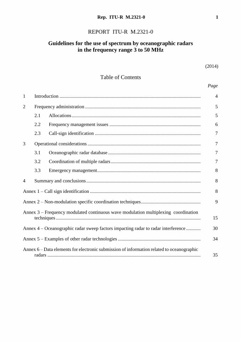
Table of Contents

Page

1 Introduction .................................................................................................................... 4

2 Frequency administration ............................................................................................... 5

2.1 Allocations .......................................................................................................... 5

2.2 Frequency management issues ........................................................................... 6

2.3 Call-sign identification ....................................................................................... 7

3 Operational considerations ............................................................................................. 7

3.1 Oceanographic radar database ............................................................................ 7

3.2 Coordination of multiple radars .......................................................................... 7

3.3 Emergency management ..................................................................................... 8

4 Summary and conclusions .............................................................................................. 8

Annex 1 – Call sign identification ........................................................................................... 8

Annex 2 – Non-modulation specific coordination techniques ................................................. 9

Annex 3 – Frequency modulated continuous wave modulation multiplexing coordination

techniques ....................................................................................................................... 15

Annex 4 – Oceanographic radar sweep factors impacting radar to radar interference ............ 30

Annex 5 – Examples of other radar technologies .................................................................... 34

Annex 6 – Data elements for electronic submission of information related to oceanographic

radars .............................................................................................................................. 35

2 Rep. ITU-R M.2321-0

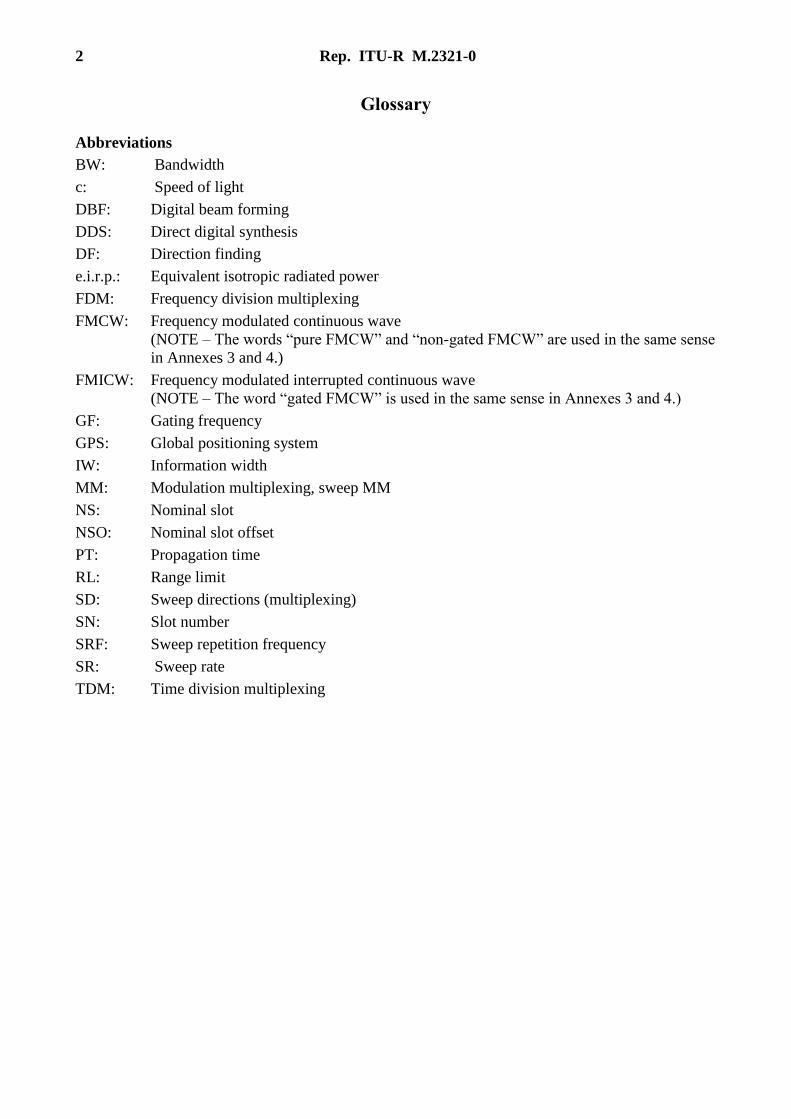
Glossary

Abbreviations

BW: Bandwidth

c: Speed of light

DBF: Digital beam forming

DDS: Direct digital synthesis

DF: Direction finding

e.i.r.p.: Equivalent isotropic radiated power

FDM: Frequency division multiplexing

FMCW: Frequency modulated continuous wave

(NOTE – The words “pure FMCW” and “non-gated FMCW” are used in the same sense

in Annexes 3 and 4.)

FMICW: Frequency modulated interrupted continuous wave

(NOTE – The word “gated FMCW” is used in the same sense in Annexes 3 and 4.)

GF: Gating frequency

GPS: Global positioning system

IW: Information width

MM: Modulation multiplexing, sweep MM

NS: Nominal slot

NSO: Nominal slot offset

PT: Propagation time

RL: Range limit

SD: Sweep directions (multiplexing)

SN: Slot number

SRF: Sweep repetition frequency

SR: Sweep rate

TDM: Time division multiplexing

Rep. ITU-R M.2321-0 3

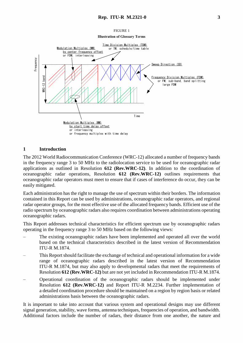
FIGURE 1

Illustration of Glossary Terms

Time

Frequency

Time Division Multiplex (TDM) or TM, schedule/time table Modulation Multiplex (MM)

by center frequency offset or FDM, interleaving

Modulation Multiplex (MM) by start time delay offset or interleaving or frequency multiplex with time delay

Frequency Division Multiplex (FDM) or FM, sub-band, band splitting large FDM

Sweep Direction (SD)

WRC-

12 band

1 Introduction

The 2012 World Radiocommunication Conference (WRC-12) allocated a number of frequency bands

in the frequency range 3 to 50 MHz to the radiolocation service to be used for oceanographic radar

applications as outlined in Resolution 612 (Rev.WRC-12). In addition to the coordination of

oceanographic radar operations, Resolution 612 (Rev.WRC-12) outlines requirements that

oceanographic radar operators must meet to ensure that if cases of interference do occur, they can be

easily mitigated.

Each administration has the right to manage the use of spectrum within their borders. The information

contained in this Report can be used by administrations, oceanographic radar operators, and regional

radar operator groups, for the most effective use of the allocated frequency bands. Efficient use of the

radio spectrum by oceanographic radars also requires coordination between administrations operating

oceanographic radars.

This Report addresses technical characteristics for efficient spectrum use by oceanographic radars

operating in the frequency range 3 to 50 MHz based on the following views:

– The existing oceanographic radars have been implemented and operated all over the world

based on the technical characteristics described in the latest version of Recommendation

ITU-R M.1874.

– This Report should facilitate the exchange of technical and operational information for a wide

range of oceanographic radars described in the latest version of Recommendation

ITU-R M.1874, but may also apply to developmental radars that meet the requirements of

Resolution 612 (Rev.WRC-12) but are not yet included in Recommendation ITU-R M.1874.

– Operational coordination of the oceanographic radars should be implemented under

Resolution 612 (Rev.WRC-12) and Report ITU-R M.2234. Further implementation of

a detailed coordination procedure should be maintained on a region by region basis or related

administrations basis between the oceanographic radars.

It is important to take into account that various system and operational designs may use different

signal generation, stability, wave forms, antenna techniques, frequencies of operation, and bandwidth.

Additional factors include the number of radars, their distance from one another, the nature and

4 Rep. ITU-R M.2321-0

geometry of paths (sea, land, mixed) between them, the required timeliness and duration period of

radar output data, their mode of operation (whether or not multi-static operations among neighbouring

radars is planned), required multi-function capability, intended application(s) of the oceanographic

radar network, the spatial resolution needed to achieve intended application goals, the signal

parameters of nearby radars that have already been assigned a frequency and the need to mitigate

other-source interference within allocated bands. All of these factors affect the frequency sharing

conditions

Oceanographic radars may require coordination and use of sharing techniques outlined in this report

when they have separation distances less than 920 km while operating at frequencies near 5 MHz,

670 km while operating at frequencies near 9 MHz, 520 km while operating in the 13 to 17 MHz

range, and 320 km above 20 MHz.

The coordination technique used for each radar should be selected or defined regarding its operation,

frequency parameter, output power, environment, number of radars simultaneously operated, and

cost, across multiple technologies.

At frequencies below 20 MHz, where available allocated spectrum is limited, division of these among

different users is desirable via FDM. However, too narrow a bandwidth per radar can result in too

large a radar cell to be useful for many applications. This leads one toward operation via several

techniques (e.g. MM (modulation multiplexing) and other techniques).

At frequencies above 20 MHz, mutual interference among nearby radars becomes considerably less

limiting. Radars can be more closely packed together without needing precise timing because

simultaneous operation on the same frequency becomes possible.

Descriptions of coordination technologies such TDM, FDM and beam steering are discussed

in Annex 2. Modulation multiplexing techniques are discussed in Annex 3.

Other annexes detail complementary techniques: Annex 1 describes a technique that could be used

for call sign identification; Annex 4 addresses oceanographic radar sweep factors, Annex 5 describes

radar technologies other than FMCW and Annex 6 contains a detailed description of the data elements

used for electronic submission of information related to oceanographic radars.

2 Frequency administration

In order to effectively use the spectrum that has been allocated for oceanographic radar operations, a

global approach will need to be taken to the management of the available spectrum.

– Administrations should coordinate with each other under resolves 6 of

Resolution 612 (Rev.WRC-12), which defines the separation distances between

the oceanographic radar and the border of other countries, and Report ITU-R M.2234;

– Frequency assignment to the radiolocation service to be used for the oceanographic radar of

each country should be managed by each administration.

2.1 Allocations

A number of frequency bands have been allocated to the radiolocation service for operation of

oceanographic radars. The frequency bands are listed in Table 1 below. In some cases the allocated

bandwidth is not significantly larger than the typical radar transmit bandwidth for the given frequency

range of operation. Therefore careful planning and spectrum sharing between radars is required to

ensure access to the frequency bands by all oceanographic radar operators. This is especially

important for real-time operation of permanent, extended coastal networks fulfilling societal needs.

Mitigation techniques allowing for an efficient use of the allocated frequency bands for

Rep. ITU-R M.2321-0 5

oceanographic radar purposes is covered in Annexes 2, 3 and 4. Operation of experimental radars

could also use the same coordination techniques.

TABLE 1

Allocated frequency bands (kHz)

ITU

Region 1

ITU

Region 2

ITU

Region 3

4 438-4 488 (S)** 4 438-4 488 (P)** 4 438-4 488 (S)**

5 250-5 275 (S)** 5 250-5 275 (P)** 5 250-5 275 (S)**

9 305-9 355 (S)* No allocation 9 305-9 355 (S)*

13 450-13 550 (S)** 13 450-13 550 (P)** 13 450-13 550 (S)**

16 100-16 200 (S)* 16 100-16 200 (P)* 16 100-16 200 (S)*

24 450-24 600 (S)** 24 450-24 650 (P)** 24 450-24 600 (S)**

26 200-26 350 (S)** 26 200-26 420 (P)** 26 200-26 350 (S)**

39 000-39 500 (S)** No allocation 39 500-40 000 (P)**

42 000-42 500 (S)** No allocation No allocation

P – Indicates a primary allocation

S – Indicates a secondary allocation

* RR No. 5.145A states that “Stations in the radiolocation service shall not cause harmful interference to,

or claim protection from, stations operating in the fixed service. Applications of the radiolocation service

are limited to oceanographic radars operating in accordance with Resolution 612 (Rev.WRC 12).”

** RR No. 5.132A states that “Stations in the radiolocation service shall not cause harmful interference to,

or claim protection from, stations operating in the fixed or mobile services. Applications of the

radiolocation service are limited to oceanographic radars operating in accordance with Resolution 612

(Rev.WRC 12).”

RR No. 5.161A: Additional allocation: in Korea (Rep. of) and the United States, the frequency bands

41.015-41.665 MHz and 43.35-44 MHz are also allocated to the radiolocation service on a primary

basis. Stations in the radiolocation service shall not cause harmful interference to, or claim protection

from, stations operating in the fixed or mobile services. Applications of the radiolocation service are

limited to oceanographic radars operating in accordance with Resolution 612 (Rev.WRC-12).

Secondary stations can claim protection, however, from harmful interference from stations of

the same or other secondary service(s) to which frequencies may be assigned at a later date

(Ref. RR Volume 1 – RR No. 5.31).

2.2 Frequency management issues

As of 2012 there are approximately 500 oceanographic radars in operation. The majority of these

radars are operated worldwide in real time and the expectation is that their numbers will continue

to increase. In the past, the majority of these systems were operated under assignments based on

RR No. 4.4. Total spectral usage was spread over approximately 7 MHz of spectrum. As a result of

Resolution 612 (Rev.WRC-12), nearly all of these radars operating on a permanent basis below 30

MHz are now required to fit within allocated frequency bands totalling no greater than 700 kHz.

Furthermore, from an operational perspective, it has been shown that a majority of radars must operate

within a 200 kHz bandwidth between 10 and 20 MHz in order to meet their mission objectives. This

means that many radars must operate simultaneously within the same frequency band within a

6 Rep. ITU-R M.2321-0

geographic region. Since many of these radars will be within radio reception range of each other they

can mutually interfere and impede their collective ability to perform sea state measurements. This

results in the need for coordinated operation of radar stations installed within a geographic area and

possibly under the jurisdiction of multiple administrations. In order to achieve interference free

operation a variety of different system parameters and design options need to be taken into account.

In addition to coordination with other allocated services and between oceanographic radar operators,

a requirement imposed by Resolution 612 (Rev.WRC-12) requires that oceanographic radar stations

must transmit station identification in international Morse code at manual speed, at the end of each

data acquisition cycle, but at an interval of no more than 20 minutes. In practice the purpose of the

call sign is to identify a station that may be interfering with other radio services.

2.3 Call-sign identification

A call sign in Morse code should be detectable by international monitoring stations (Article 16 of the

RR). Experienced Morse code listeners can receive at rates of 15 words per minute or more. In

accordance with Resolution 612 (Rev.WRC-12) the call sign shall be transmitted on the assigned

frequency. The call sign signal heard by the impacted radio should be transmitted at the same power

level as the normal radar signal. The details that are associated with several call sign identification

techniques can be found in Annex 1.

3 Operational considerations

3.1 Oceanographic radar database

WRC-12 allocated a number of frequency bands in the frequency range of 3-50 MHz to

the radiolocation service limited to oceanographic radars operating in accordance with Resolution 612

(Rev.WRC-12). The Resolution resolves, inter alia, that the oceanographic radars shall be

coordinated with neighboring administrations if they are located at certain distances to the border.

The establishment of a database on existing and planned oceanographic radars may considerably

facilitate this coordination process. Such a database would serve as reference information for

coordination purposes and would not have any regulatory status. Administrations wishing to obtain

the status of international recognition for their radars still need to record the frequency assignments

in the master international frequency register.

Given a worldwide nature of this potential database and a significant involvement of the ITU in the

regulation of oceanographic radars, it might be appropriate that such a database is established and

maintained by the Radiocommunication Bureau and populated by the ITU administrations.

The data elements of the database are described in Annex 6.

3.2 Coordination of multiple radars

Taking into account the present development and usage of oceanographic radars, as well as

the expectation that their numbers will continue to increase, considerations that are fundamental to

any coordination effort and be found in Annex 2 “Non-modulation specific coordination techniques”

and Annex 3 “Frequency modulated continuous wave modulation multiplexing coordination

techniques”.

The bandwidth of oceanographic radars determines the range cell size, where an inverse relationship

exists between bandwidth and range cell size. For example, a 50 kHz bandwidth leads to a 3 km range

cell; 150 kHz leads to a 1 km range cell, etc. Selecting the appropriate bandwidth is a trade-off

between achieving the best possible range resolution while minimizing bandwidth utilization. Radars

which are operating at the same frequency could, depending upon the stability, modulation and

Rep. ITU-R M.2321-0 7

bandwidth, have a potential for interfering with one another’s operation. A detailed discussion of the

impact that these factors could have on an operational network can be found in Annex 4 –

“Oceanographic radar sweep factors impacting radar to radar interference”.

3.3 Emergency management

Oceanographic radars are generally designed for reporting current data and sea state once or twice an

hour. In the case an emergency event, (e.g. tsunami, search and rescue, oil spills, etc.) the radars are

required to report data immediately and continuously using short time intervals without interference

from other radars which are located within the same region.

Therefore, when several radars coexist in the same region and there is a possibility of interference

between them, the following methods are recommended for emergency operation:

1) To prioritize in advance the radars for emergency use in this area.

2) To stop transmission of the radars with low priority for an appropriate period after the

emergency event occurs.

In order for the above arrangement in certain area, coordination among the radar operators may be

required. This depends on licensing policy of each Administration. This method is applicable when

the radar is required to perform continuous monitoring immediately after the emergency event.

4 Summary and conclusions

Efficient use of the radio spectrum by oceanographic radars requires coordination between

Administrations authorizing the operation of these radars. The information that has been presented in

this Report and its’ annexes can be used by Administrations, oceanographic radar operators, spectrum

managers, regulators and regional operator groups to achieve effective use of the allocated frequency

bands.

Annex 1

Call sign identification

1 A1A/A2A Method

Operation of the oceanographic radar should be in accordance with Resolution 612 (Rev.WRC-12),

which resolves that each oceanographic radar station shall transmit station identification (call sign)

on the assigned frequency, in international Morse code at manual speed, at the end of each data

acquisition cycle, but at an interval of no more than 20 minutes.

Table 1 shows requirements for transmitting the call-sign under the Resolution 612 (Rev.WRC-12).

Based on this, the call-sign is transmitted in standard CW (A1A/A2A) signal, and can be demodulated

by a general HF receiver such as a receiver with single side band (SSB) reception. This method is in

accordance with Recommendation ITU-R M.1677.

8 Rep. ITU-R M.2321-0

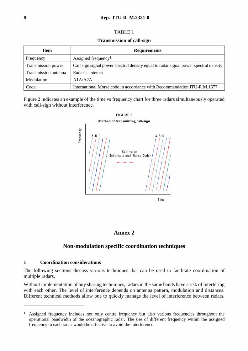
TABLE 1

Transmission of call-sign

Item Requirements

Frequency Assigned frequency1

Transmission power Call sign signal power spectral density equal to radar signal power spectral density

Transmission antenna Radar’s antenna

Modulation A1A/A2A

Code International Morse code in accordance with Recommendation ITU-R M.1677

Figure 2 indicates an example of the time vs frequency chart for three radars simultaneously operated

with call-sign without interference.

FIGURE 2

Method of transmitting call-sign

Annex 2

Non-modulation specific coordination techniques

1 Coordination considerations

The following sections discuss various techniques that can be used to facilitate coordination of

multiple radars.

Without implementation of any sharing techniques, radars in the same bands have a risk of interfering

with each other. The level of interference depends on antenna pattern, modulation and distances.

Different technical methods allow one to quickly manage the level of interference between radars,

1 Assigned frequency includes not only centre frequency but also various frequencies throughout the

operational bandwidth of the oceanographic radar. The use of different frequency within the assigned

frequency to each radar would be effective to avoid the interference.

Time

Freq

uenc

y

Call-sign(International Morse Code)

A B C A B C

Rep. ITU-R M.2321-0 9

especially if users and operators try to perform some planning and identify the best method before

starting the deployment process.

For radars using the same family of modulation, “fine tuning and fine synchronization” methods allow

optimization of coordination, and yield increased radar capacity in the frequency band. This is the

subject of the Annex 3 for the frequency modulated continuous wave (FMCW) class of modulation.

For sequence coded radars of the Annex 5, the use of the same family of orthogonal sequences may

be a way to obtain a higher radar capacity.

The approaches described in the following sections in this Annex have the advantage of not putting

any restrictions on modulation schemes or waveforms. The three approaches are independent and can

be combined. Nevertheless, considering the potential need, they yield a limited number of

independent channels in comparison to modulation multiplexing (Annex 3).

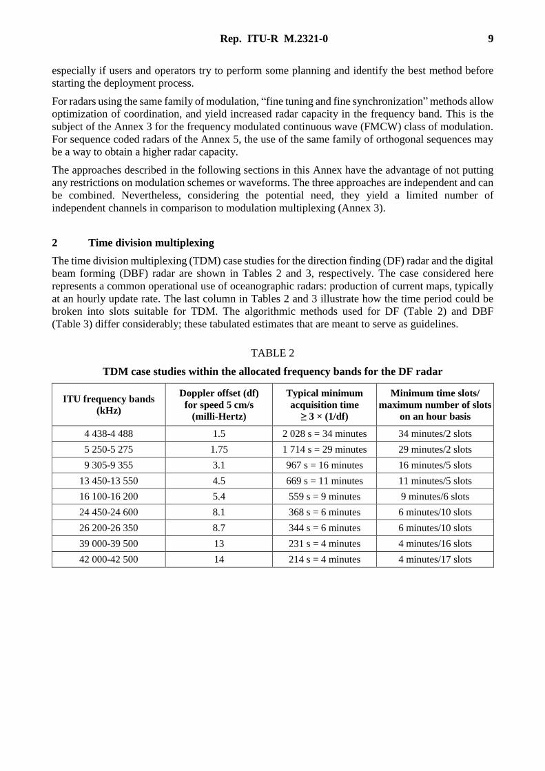
2 Time division multiplexing

The time division multiplexing (TDM) case studies for the direction finding (DF) radar and the digital

beam forming (DBF) radar are shown in Tables 2 and 3, respectively. The case considered here

represents a common operational use of oceanographic radars: production of current maps, typically

at an hourly update rate. The last column in Tables 2 and 3 illustrate how the time period could be

broken into slots suitable for TDM. The algorithmic methods used for DF (Table 2) and DBF

(Table 3) differ considerably; these tabulated estimates that are meant to serve as guidelines.

TABLE 2

TDM case studies within the allocated frequency bands for the DF radar

ITU frequency bands

(kHz)

Doppler offset (df)

for speed 5 cm/s

(milli-Hertz)

Typical minimum

acquisition time

≥ 3 × (1/df)

Minimum time slots/

maximum number of slots

on an hour basis

4 438-4 488 1.5 2 028 s = 34 minutes 34 minutes/2 slots

5 250-5 275 1.75 1 714 s = 29 minutes 29 minutes/2 slots

9 305-9 355 3.1 967 s = 16 minutes 16 minutes/5 slots





39 000-39 500 13 231 s = 4 minutes 4 minutes/16 slots

42 000-42 500 14 214 s = 4 minutes 4 minutes/17 slots

10 Rep. ITU-R M.2321-0

TABLE 3

TDM case studies within the allocated frequency bands for the DBF radar

ITU frequency bands

(kHz)

Doppler offset (df)

for speed 5 cm/s

(milli-Hertz)

Proposed minimum

acquisition time

≥ (1/df)

Minimum time slots/

maximum number of slots

on an hour basis



9 305-9 355 3.1 322 s = 5.4 minutes 5.4 minutes/11 slots





39 000-39 500 13 77 s = 1.3 minutes 1.3 minutes/47 slots

42 000-42 500 14 71 s = 1.2 minutes 1.2 minutes/50 slots

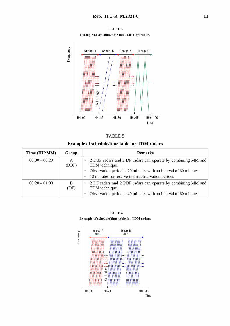
TDM can be applied in various time patterns and can be used to coordinate systems of different brands

and modulation types, Table 4 and Fig. 3 show an example of schedule/time table for the TDM radars

combining the modulation multiplexing (MM) (refer to Annex 3) and the TDM technique. If

operational coordination between these radars is carried out based on Table 4, flexible multiplexing

can be realized between several radars with different technical characteristics as shown in Fig. 3. The

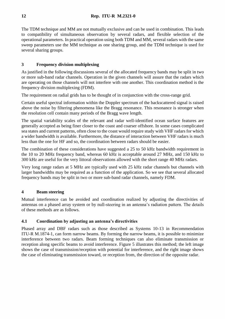
TDM technique makes it possible to select the parameters flexibly. Table 5 and Fig. 4 show another

example of two DBF radars and two DF radars operation in the same area.

TABLE 4

Example of schedule/time table for TDM radars

Time (HH:MM) Group Remarks

00:00 – 00:15 A • Multiple radars can operate by combining MM and TDM technique.

• Observation period is 15 minutes with an interval of 30 minutes.

00:15 – 00:30 B • Multiple radars can operate by combining MM and TDM technique.


00:30 – 00:45 A Second window for Group A.

00:45 – 01:00 C For experimental radars with characteristics that do not conform to

Group A or Group B.

Rep. ITU-R M.2321-0 11

FIGURE 3


Time

Frequency

Group A

HH:00 HH:15 HH:30 HH:45

Call-sign

Group B Group A Group C

HH+1:00

TABLE 5


Time (HH:MM) Group Remarks

00:00 – 00:20 A

(DBF)

• 2 DBF radars and 2 DF radars can operate by combining MM and

TDM technique.


• 10 minutes for reserve in this observation periods

00:20 – 01:00 B

(DF)

• 2 DF radars and 2 DBF radars can operate by combining MM and

TDM technique.


FIGURE 4


Time

Frequency Group A(DBF)

HH:00 HH:20

Group B(DF)

HH+1:00

Call-sign

12 Rep. ITU-R M.2321-0

The TDM technique and MM are not mutually exclusive and can be used in combination. This leads

to compatibility of simultaneous observation by several radars, and flexible selection of the

operational parameters. In practical operation using both TDM and MM, several radars with the same

sweep parameters use the MM technique as one sharing group, and the TDM technique is used for

several sharing groups.

3 Frequency division multiplexing

As justified in the following discussions several of the allocated frequency bands may be split in two

or more sub-band radar channels. Operation in the given channels will assure that the radars which

are operating on those channels will not interfere with one another. This coordination method is the

frequency division multiplexing (FDM).

The requirement on radial grids has to be thought of in conjunction with the cross-range grid.

Certain useful spectral information within the Doppler spectrum of the backscattered signal is raised

above the noise by filtering phenomena like the Bragg resonance. This resonance is stronger when

the resolution cell contain many periods of the Bragg wave length.

The spatial variability scales of the relevant and radar well-identified ocean surface features are

generally accepted as being finer closer to the coast and coarser offshore. In some cases complicated

sea states and current patterns, often close to the coast would require study with VHF radars for which

a wider bandwidth is available. Furthermore, the distance of interaction between VHF radars is much

less than the one for HF and so, the coordination between radars should be easier.

The combination of these considerations have suggested a 25 to 50 kHz bandwidth requirement in

the 10 to 20 MHz frequency band, whereas 60 kHz is acceptable around 27 MHz, and 150 kHz to

300 kHz are useful for the very littoral observations allowed with the short range 40 MHz radars.

Very long range radars at 5 MHz are typically used with 25 kHz radar channels but channels with

larger bandwidths may be required as a function of the application. So we see that several allocated

frequency bands may be split in two or more sub-band radar channels, namely FDM.

4 Beam steering

Mutual interference can be avoided and coordination realized by adjusting the directivities of

antennas on a phased array system or by null-steering in an antenna’s radiation pattern. The details

of these methods are as follows.

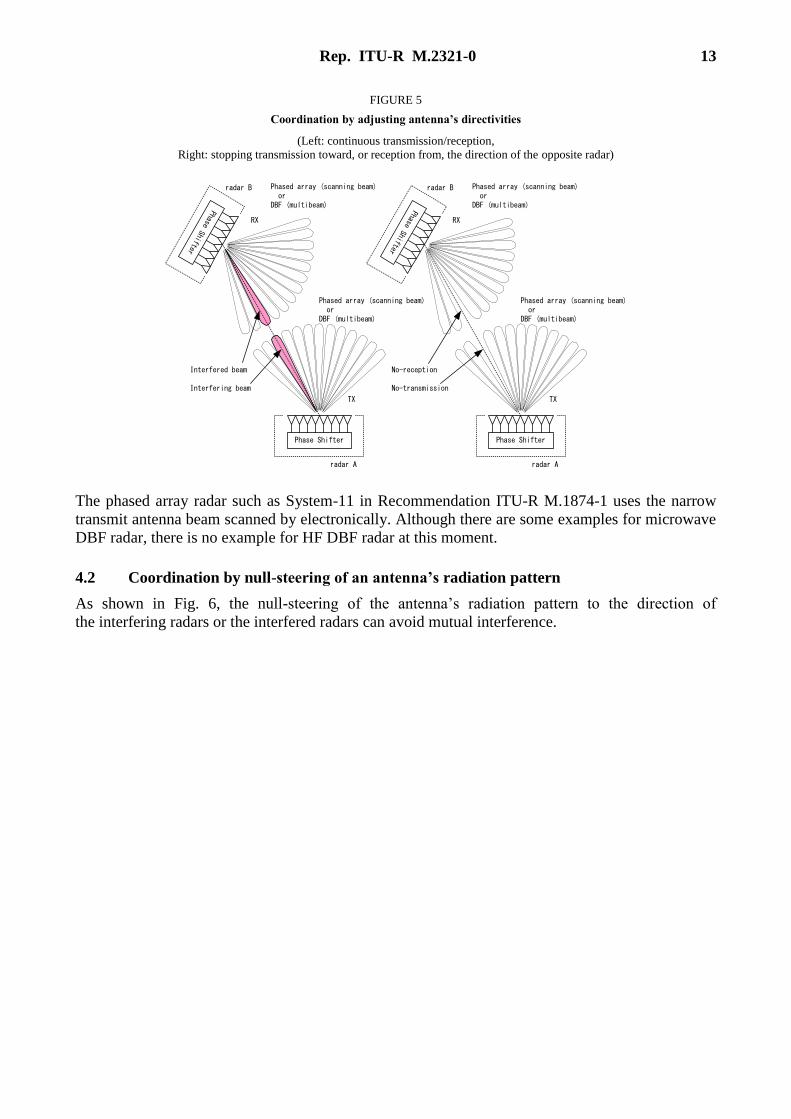
4.1 Coordination by adjusting an antenna’s directivities

Phased array and DBF radars such as those described as Systems 10-13 in Recommendation

ITU-R M.1874-1, can form narrow beams. By forming the narrow beams, it is possible to minimize

interference between two radars. Beam forming techniques can also eliminate transmission or

reception along specific beams to avoid interference. Figure 5 illustrates this method; the left image

shows the case of transmission/reception with potential for interference, and the right image shows

the case of eliminating transmission toward, or reception from, the direction of the opposite radar.

Rep. ITU-R M.2321-0 13

FIGURE 5

Coordination by adjusting antenna’s directivities

(Left: continuous transmission/reception,

Right: stopping transmission toward, or reception from, the direction of the opposite radar)

Phase Shifter

Phase Shifter

Phase Shifter

Phase Shifter

radar A

radar B

Interfered beam

Interfering beam

No-reception

No-transmission

radar A

radar B

TX

RX

TX

RX

Phased array (scanning beam) orDBF (multibeam)




The phased array radar such as System-11 in Recommendation ITU-R M.1874-1 uses the narrow

transmit antenna beam scanned by electronically. Although there are some examples for microwave

DBF radar, there is no example for HF DBF radar at this moment.

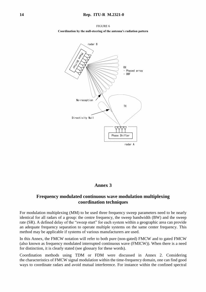
4.2 Coordination by null-steering of an antenna’s radiation pattern

As shown in Fig. 6, the null-steering of the antenna’s radiation pattern to the direction of

the interfering radars or the interfered radars can avoid mutual interference.

14 Rep. ITU-R M.2321-0

FIGURE 6

Coordination by the null-steering of the antenna’s radiation pattern

Phase Shifter

Directivity Null

radar A

radar B

Phase Shifter

TX

No-reception

RX- Phased array- DBF

Annex 3

Frequency modulated continuous wave modulation multiplexing

coordination techniques

For modulation multiplexing (MM) to be used three frequency sweep parameters need to be nearly

identical for all radars of a group: the centre frequency, the sweep bandwidth (BW) and the sweep

rate (SR). A defined delay of the “sweep start” for each system within a geographic area can provide

an adequate frequency separation to operate multiple systems on the same center frequency. This

method may be applicable if systems of various manufacturers are used.

In this Annex, the FMCW notation will refer to both pure (non-gated) FMCW and to gated FMCW

(also known as frequency modulated interrupted continuous wave (FMICW)). When there is a need

for distinction, it is clearly stated (see glossary for these words).

Coordination methods using TDM or FDM were discussed in Annex 2. Considering

the characteristics of FMCW signal modulation within the time-frequency domain, one can find good

ways to coordinate radars and avoid mutual interference. For instance within the confined spectral

Rep. ITU-R M.2321-0 15

space of the allocated frequency bands, or when TDM is not an acceptable solution, one should

consider the MM approach.

1 Method 1 (Modulation multiplexing with slot allocation)

1.1 Modulation multiplexing within the frequency modulated continuous wave

linear sweeps

In this section, two simple and powerful coordination methods of the radar sweeps are presented.

They are not manufacturer specific, and can be achieved within available clock stability constraints.

They yield, for a given geographic area, a capacity over 25 radar stations. Finer sweep coordination

may facilitate the deployment of an even larger number of stations, as well as bi-static and multi-static

systems.

In the linear frequency sweep that is used for FMCW oceanographic radar, the carrier frequency slope

(in Hz per second) which is called the SR is constant during the sweep, and discontinuity only occurs

during the very short flyback.

The SR is the product of the bandwidth (BW) and SRF. The BW is related to the range resolution,

whereas the SRF defines the Doppler unambiguity and it has to be chosen in relation to the maximum

speed of the targets within the cell (e.g. Bragg waves, current, moving vessels, etc.).

The SR, in combination with the selected SRF, is in fact, the key parameter for FMCW radar

coordination. In the time-frequency domain, the sweeping FMCW carrier is described by a straight

line, whether it is ascending or descending, according to the sweep direction.

In this time-frequency space, the delayed sea scattered signals are occupying a close-by information

band on one side of the carrier. The backscatter offset frequency is the product of the SR by

the propagation delay. The maximum information bandwidth is determined by the maximum

expected range. The signals from the farther distances are the weaker ones. The full information

bandwidth must not be contaminated. Thus, radar channels are the useful spectral sweeps that cross

the time-frequency space.

For instance, with a 100 kHz/s SR and a 150 km maximum expected range, the maximum propagation

delay is 1 millisecond and the information bandwidth is 100 Hz.

Two parallel well separated spectral sweep generated with the same SR and SRF will never overlap,

except during the sweep flybacks. Flybacks are made very short and significantly reduce interactions

between FMCW radars.

Considerations leading to the SRF selection and sweep-start offset selection, as well as tradeoffs, will

be discussed later. The optimum choice for SR depends on the allocated frequency band, but its value

should be agreed upon over areas where several radars are or will be operated. Once a SRF and a BW

are chosen, the SR is also defined by the direct calculation SR = SRF × BW. Under these conditions

FMCW radar coordination by MM is achieved by the selection of an inter-radar spectral sweep offset

acting as a spectral separation “distance”, wide enough to isolate the information bandwidth.

Whereas very well synchronized and highly compatible radars could be operated with a very small

offset, radars with differing stabilities, drifts or hardware performance limitations may need a wider

separation. If there is an agreed upon common offset separation value, the so called nominal slot

offset (NSO) may be defined for each allocated frequency band. Once such a spectral sweep (offset)

is defined, nominal slots (NS) may be defined. The slots should be allocated on a given geographic

area basis.

There are several ways to associate a radar or groups of radars to nominal slots. The simplest way to

go is to give one radar one slot. As very highly synchronized radars will not need a large offset, and

16 Rep. ITU-R M.2321-0

as the information bandwidth are quite narrow, several well synchronized radars may be grouped

within only one such nominal slot. This technique is already applied on some radar networks.

1.2 Possible technical performance on carrier and time base stability to maintain the radar

slots

To maintain the separation between two radar spectral sweeps, we can identify two kinds of

requirement. First, the carrier accuracy and drift must be maintained to keep the required separation.

Second, the radar time base must ensure that the sweep start time accuracy is maintained. The two

needs may be simultaneously achieved through the use of a high quality master clock, but several

scenarios may also be used for resynchronization from external references. This is discussed further

in § 1.7 after technical performance has been analysed.

1.3 Compatibility of the modulation multiplexing method for pure frequency modulated

continuous wave and gated frequency modulated continuous wave radars

The compatibility for pure FMCW and gated FMCW (FMICW) is assumed. Due to their modulation

technique, FMICW transmitters produce a few sidebands. The number of these sidebands is normally

kept to a minimum by use of appropriate filtering and pulse shaping.

As a result, the data contained in the transmitters’ signal is replicated in sidebands. So the FMICW

radar produces a wider occupation of the time-frequency space. The Gating Frequency (GF), and the

gating shape determine this expansion. (See Report ITU-R M.2234.)

From a radar to radar compatibility perspective, a first cautious implementation should be considered

to maintain a larger time-frequency separation between a FMICW radar and other FMCW radars.

Several adjacent nominal slots (NS’s) may be dedicated to one FMICW radar or to a group of such

radars (see § 1.5 Annex 3).

For example, the rapid GF with respect to the slow SRF lays down a modulation pattern of circular

peaks/nulls on the received amplitude from the sea surface within the distance over which the radar

can see. The gate width and GF must be carefully designed to accommodate the expected maximum

range. For example, assume a pure FMCW radar would see out to about 75 km. Then with

square-wave gating, to match this 75 km range we need a 1 000 microsecond gating period. With the

corresponding 1 kHz GF, the gating duty factor reaches a maximum at a range of 75 km. At exactly

twice this range (150 km), the duty factor has dropped to zero, and we call this null a blind zone (it is

named range limit in Table 6, Annex 3), at and near which, targets cannot be detected. Such maxima

and blind zones repeat periodically at 150 km range intervals for this example. So a 1 kHz GF is

compatible with this range example. The correct values will inversely scale with the range limit of

the allocated band on which the radar operates (see Table 6, Annex 3).

With a smooth gating and a 50% gating duty cycle, the spectrum replica will be concentrated near the

carrier and near the sidelobes corresponding to the first odd harmonics of the GF. See Fig. 92 page

121 in Report ITU-R M.2234. With a 1 kHz GF, the first sidelobes are then sitting on both sides of

the carrier at 1 kHz, 3 kHz, 5 kHz, with decreasing amplitudes at higher baseband frequencies.

A more careful approach to avoid interference from an FMICW radar may be achieved, if the nominal

slot offset is an even harmonic of the GF, since there are no FMICW sidelobes around the even

harmonics for the 50% gating. It is found for this example that 2 kHz2 is a good candidate as a

common NSO.

2 This 2 kHz value is compatible with already available radar characteristics.

Rep. ITU-R M.2321-0 17

So, in the 13 500 MHz example below in § 1.4, we see that a FMCW may operate at least 6 kHz (i.e.

3 × NSO) away from an FMICW radar. Nevertheless, the FMICW to FMICW radar separation must

be kept about twice as wide since their relative sidelobes may overlap.

1.4 Slot allocation according to different frequency modulated continuous wave radar

technology

For each allocated frequency band, to ease the heterogeneous radar coordination, gated frequency

FMICW radars should be operated at 50% duty cycle as is stated before in § 1.3, and with a nominal

GF, compatible with the allocated frequency band range limit.

For instance, for the 13 500 MHz and at 16 100 MHz bands, with a 1 kHz GF, the NSO could be set

to 2 kHz, yielding 50 slots over both 100 kHz bandwidth.

Then, a FMICW radar or a FMICW group of synchronized radars (as described in § 1.5) could be

attributed a set of 6 to 10 slots. Some pure FMCW radars could be attributed one single slot, whereas

less stable radars could be attributed to a couple of adjacent slots.

1.5 Coordinating modulated continuous wave radar with synchronization by global

navigation satellite systems signals or other highly accurate frequency sources

If a more accurate clock stability and synchronization between radars can be achieved (as with GPS

synchronized radars), and when using radars with state machines directly driven by similar master

clocks and circuitry (typically same brand and same generation radars), then almost no relevant

relative drift will occur, and it is possible to use very close spectrum sweeps.

The number of usable information bandwidths depends on the information bandwidth and on the GF.

As the information bandwidth is on the order of 100 Hz or less, using high stability, the separation

offset can be reduced, and the band capacity is accordingly improved.

With FMICW radars, for a 1 kHz GF, within the 1 kHz gap between the carrier and the first sideband,

ten 100 Hz spectrum sweeps may be installed, this means 10 radars. But in fact, the total spectral foot

print is spreading over several kHz on both sides, due to the side lobe replication. Then several very

finely synchronized FMICW radars can be gathered in groups, but such groups have to be separated

by a gap of about 10 kHz.

1.6 Modulation multiplexing carrier offset methods

This offset can be achieved by two methods:

– offsetting the sweep central frequency;

– offsetting the sweep start time.

The two methods are briefly discussed in the next sections.

1.6.1 Modulation multiplexing by centre frequency offset

With the centre frequency offset method, as the bandwidth which is used for each of the radars is

shifted, the total bandwidth required by all radars increases with the number of radars, and the fixed

spectral sub band splitting required for FDM coordination as proposed in Annex 2 may not be

applicable to all configurations.

The advantage of this method is that all radar flybacks occur at almost the same time and this reduces,

even farther, the risk of interference. Radars with excessive carrier drift would also be easier to

identify.

18 Rep. ITU-R M.2321-0

1.6.2 Modulation multiplexing by start time delay offsets

To separate the parallel radar spectral sweeps, one can delay the different radar sweep starts by

a portion of the sweep period. Once the SR and the NSO are defined, the slot to slot start nominal

delay step is the ratio of NSO over SR. For instance, a 2 kHz NSO with a 100 kHz/s SR gives a 20 ms

start delay step. Then the slots can be defined by a slot number (SN) and the sweeps start with a delay

equals to SN × 20 ms. A common, accurate time base needs to be shared between operators in order

that the sweep start drift stability over the acquisition period should be small enough in the

comparison of the 20 ms start delay step.

As this delay method maintains the same bandwidth use independent of the number of operating

radars, it is the preferred way to generate the separation between FMCW radar sweeps. The main way

to accommodate this method is to use three identical parameters for the frequency sweeps: the center

frequency, the BW and the SRF. As a consequence, the two SR are also identical.

1.7 Carrier frequency and sweep time base accuracy and stability

Section 1.2 provided the general conditions that are required to maintain the radar slots. This section

details the calculation of the required accuracy and stability figures. It should be conducted for each

allocated band, once SR, GF and NSO are chosen.

Carrier accuracy and stability: assuming the 13.500 MHz frequency band, with a 2 kHz NSO, the

maximum allowable carrier drift could be standardized, for instance, to one third of the NSO: 650 Hz,

then the carrier accuracy and stability is 650 Hz / 13 MHz, that is just about 50 ppm. The maximum

allowable carrier drift is such that two operating radars will not overlap their information sweeps.

Sweep time base: assuming the 13.500 MHz frequency band, and a 100 kHz/s SR, we found that

the sweep start delay offset is equal to 2 kHz/100 kHz/s = 20 ms. Assuming a maximum allowable

drift of one third of the NSO, we find a maximum start drift of 6 ms over the full acquisition period,

or between two sweeps. For an acquisition or resynchronization interval of 10 minutes, the relative

clock to clock limit is equal to 6/(10 × 60 × 1 000), i.e. a 10 ppm requirement. For a one hour

acquisition or resynchronization interval, the requirement is 1.5 ppm.

If both the carrier generator and sweep timing are driven from the same time base, then the most

stringent requirement has to be chosen.

For some existing radars those figures may be difficult to achieve. Instead of defining a less stringent

NSO to accommodate them, one should adopt reasonably fine NSO, and allocate multiple successive

slots to those radars operating at lesser accuracy, as stated before in § 1.4 of this Annex.

1.8 Band capacity using the sweep offset modulation multiplexing method

Using the 13.500 MHz example from the previous section, i.e. a slot offset of 2 kHz, we see

that 25 radars (or groups of radars) can operate together within the same area within each of two

50 kHz sub-bands (yielding a total of 50 radars over the full width).

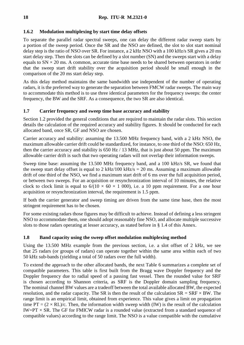
To extend the approach to the other allocated bands, the next Table 6 summarizes a complete set of

compatible parameters. This table is first built from the Bragg wave Doppler frequency and the

Doppler frequency due to radial speed of a passing fast vessel. Then the rounded value for SRF

is chosen according to Shannon criteria, as SRF is the Doppler domain sampling frequency.

The nominal channel BW values are a tradeoff between the total available allocated BW, the expected

resolution, and the radar capacity. The SR is then the result of the calculation SR = SRF × BW. The

range limit is an empirical limit, obtained from experience. This value gives a limit on propagation

time PT = (2 × RL)/c. Then, the information width sweep width (IW) is the result of the calculation

IW=PT × SR. The GF for FMICW radar is a rounded value (extracted from a standard sequence of

compatible values) according to the range limit. The NSO is a value compatible with the cumulative

Rep. ITU-R M.2321-0 19

IW, GF harmonics consideration, general clock drift consideration, and the goal for a good allocated

band capacity. Then, the geographic area radar capacity per channel is the ratio between the channel

BW and the NSO.

TABLE 6

Example of a set of parameters compatible with MM

Allocated

Band

FBragg FDopp

for a

20

knot

vessel

Nominal

sweep

repetition

Freq.

(SRF)

Nominal

channel

BW*

Nominal

SR

Range

limit

Info.

band

width

Nominal

gating

freq.

(GF)

NSO Area

radar

capacity

per

channel

Area

radar

capacity

per

allocated

band

kHz Hz Hz Hz kHz kHz/s km Hz Hz kHz

4 438-4 488 0.21 0.3 1 25 25 600 100 250 2 12 24

5 250-5 275 0.23 0.3 1 25 25 600 100 250 2 12 12

9 305-9 355 0.30 0.6 2 25 50 300 100 500 2 12 24

13 450-13 550 0.37 0.9 2 50 100 150 100 500 2 25 50

16 100-16 200 0.40 1.1 2 50 100 150 100 1 000 2 25 50

24 450-24 600 0.50 1.5 4 75 300 100 180 1 000 2 37 74

26 200-26 350 0.51 1.8 4 75 300 100 180 1 000 2 37 74

39 000-39 500 0.63 2.7 4 (or 8) 250 1 000 50 330 2 000 8 32 64

42 000-42 500 0.65 2.8 4 (or 8) 250 1 000 50 330 2 000 8 32 64

* There may be more than one channel per allocated frequency band.

2 Method 2 (Modulation multiplexing with 50 ppm stability3)

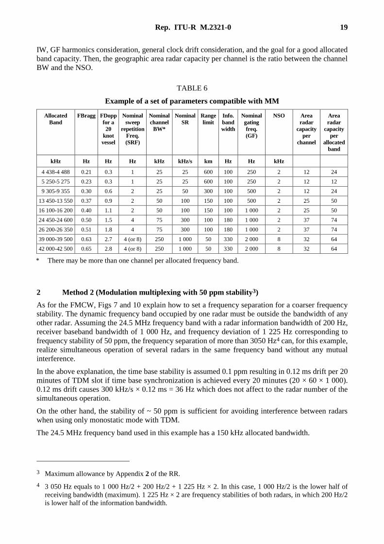
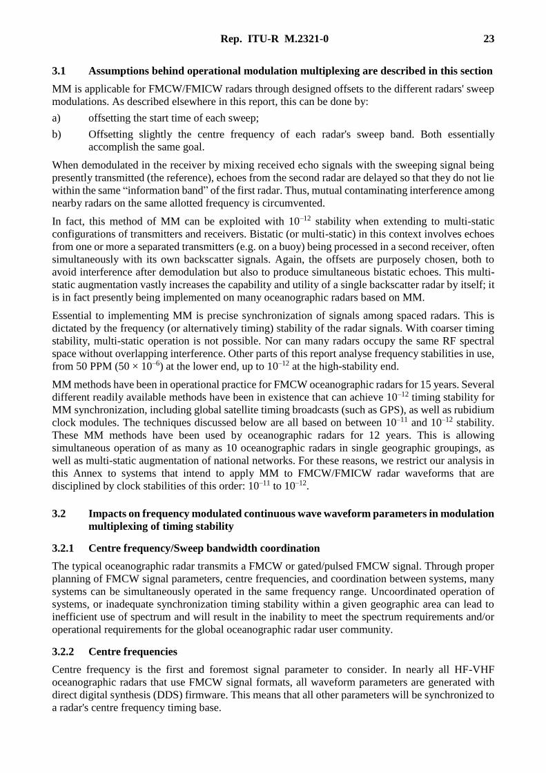
As for the FMCW, Figs 7 and 10 explain how to set a frequency separation for a coarser frequency

stability. The dynamic frequency band occupied by one radar must be outside the bandwidth of any

other radar. Assuming the 24.5 MHz frequency band with a radar information bandwidth of 200 Hz,

receiver baseband bandwidth of 1 000 Hz, and frequency deviation of 1 225 Hz corresponding to

frequency stability of 50 ppm, the frequency separation of more than 3050 Hz4 can, for this example,

realize simultaneous operation of several radars in the same frequency band without any mutual

interference.

In the above explanation, the time base stability is assumed 0.1 ppm resulting in 0.12 ms drift per 20

minutes of TDM slot if time base synchronization is achieved every 20 minutes (20 × 60 × 1 000).

0.12 ms drift causes 300 kHz/s × 0.12 ms = 36 Hz which does not affect to the radar number of the

simultaneous operation.

On the other hand, the stability of ~ 50 ppm is sufficient for avoiding interference between radars

when using only monostatic mode with TDM.

The 24.5 MHz frequency band used in this example has a 150 kHz allocated bandwidth.

3 Maximum allowance by Appendix 2 of the RR.

4 3 050 Hz equals to 1 000 Hz/2 + 200 Hz/2 + 1 225 Hz × 2. In this case, 1 000 Hz/2 is the lower half of

receiving bandwidth (maximum). 1 225 Hz × 2 are frequency stabilities of both radars, in which 200 Hz/2

is lower half of the information bandwidth.

20 Rep. ITU-R M.2321-0

In case of FMCW monostatic mode, referring Figs 7 and 10, 49 radars (= 150 kHz/3 050 Hz) can be

simultaneously operated with 50 ppm stability.

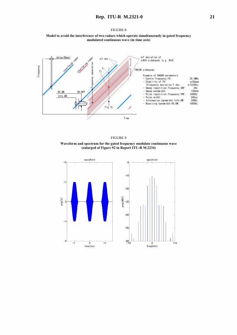
In case of FMICW monostatic mode, referring to Figs 8 and 11, 16 radars (= Sweep bandwidth /(pulse

repletion frequency × 6 + frequency separation) = 150 kHz/(1 kHz × 6 + 3.05 kHz)) can be

simultaneously operated with 50 ppm stability.

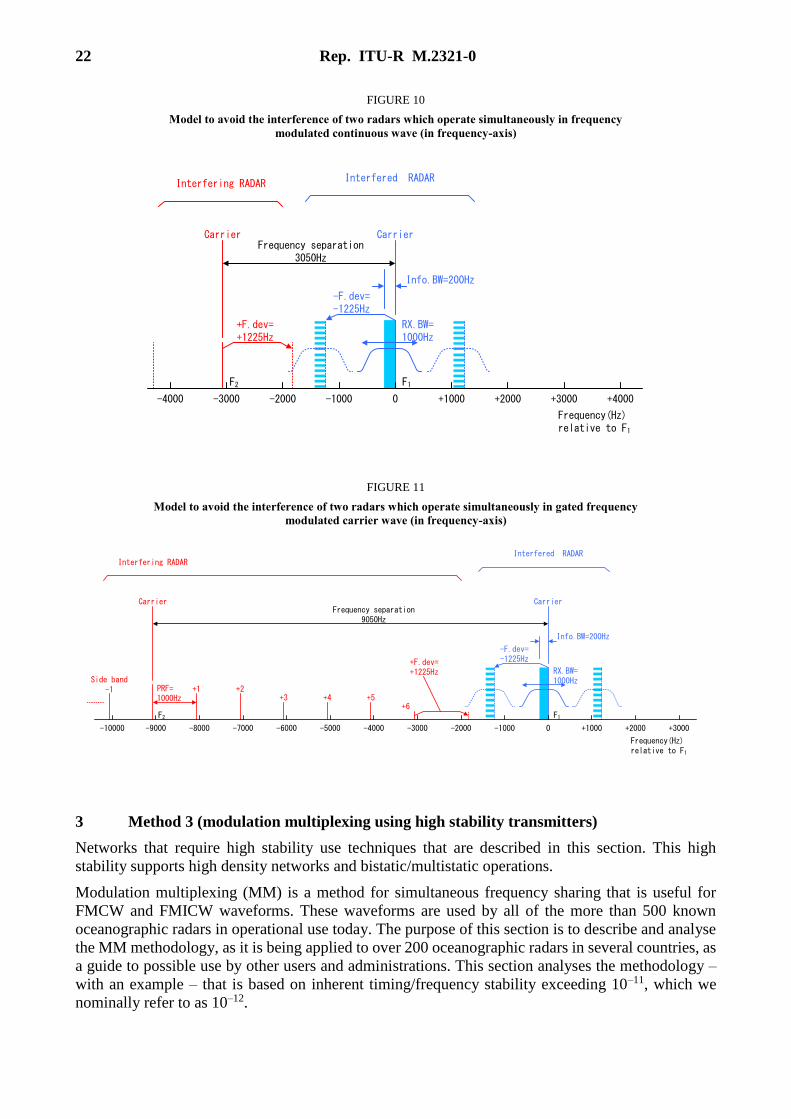
As for FMICW, it is necessary to take into account higher order harmonics of the GF as mentioned

in § 1.3 of Annex 3 and are shown in Figs 8, 9 and 11. Its waveform and spectrum are shown as Fig. 9

which is an enlargement of Fig. 92 in Report ITU-R M.2234. Figures 9 and 11 explains how to

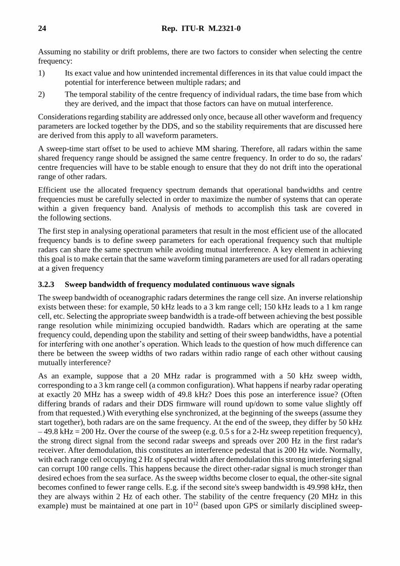
separate the frequency when not more than six harmonics are taken into account. In this case, the

separation frequency is 9 050 Hz (= 1 000 Hz × 6 + 1 000 Hz/2 + 200 Hz/2 + 1 225 Hz × 2) with

using the above mentioned FMCW parameters and 1 000 Hz of the GF. In the above explanation, the

clock stability is assumed 0.1 ppm and the drift caused by sweep rate is 36 Hz. This value does not

affect the number radars in simultaneous operation.

FIGURE 7

Model to avoid the interference of two radars which operate simultaneously in frequency

modulated continuous wave (in time axis)

interfered radar

interfering radar

Example of RADAR parameters- Centre frequency F0: 24.5MHz- Stability of F0: ±50ppm (Frequency deviation F.dev: ±1225Hz)- Sweep repetition frequency SRF: 2Hz- Sweep bandwidth: 150kHz- Information bandwidth Info.BW: 200Hz- Receiving bandwidth RX.BW: 1000Hz

±F.dev

Frequency separation

delay(Rmax)

Time

Frequency

RX-BPFFig.1D

±F.dev

RX.BW

Info.BW

F1F2

Rep. ITU-R M.2321-0 21

FIGURE 8

Model to avoid the interference of two radars which operate simultaneously in gated frequency

modulated continuous wave (in time axis)

Example of RADAR parameters- Centre frequency F0: 24.5MHz- Stability of F0: ±50ppm (Frequency deviation F.dev: ±1225Hz)- Sweep repetition frequency SRF: 2Hz- Sweep bandwidth: 150kHz- Pulse repetition frequency PRF: 1000Hz- Pulse width: 500us- Information bandwidth Info.BW: 200Hz- Receiving bandwidth RX.BW: 1000Hz

Frequency separation

Time

Frequency

FMICW sidebands

Fig.1E

delay(Rmax)

interfered radar

interfering radar ±F.deviation of

±Nth sidebands (e.g. N=6)

RX-BPFRX.BW

Info.BW

±F.dev

F1F2

FIGURE 9

Waveform and spectrum for the gated frequency modulate continuous wave

(enlarged of Figure 92 in Report ITU-R M.2234)

22 Rep. ITU-R M.2321-0

FIGURE 10

Model to avoid the interference of two radars which operate simultaneously in frequency

modulated continuous wave (in frequency-axis)

0-1000-2000-3000

Frequency separation3050Hz

RX.BW=1000Hz

Info.BW=200Hz

Carrier

-4000 +1000 +2000 +3000 +4000

Interfered　RADARInterfering RADAR

Carrier

+F.dev=+1225Hz

Frequency(Hz)relative to F1

-F.dev=-1225Hz

F1F2

FIGURE 11

Model to avoid the interference of two radars which operate simultaneously in gated frequency

modulated carrier wave (in frequency-axis)

0-1000-2000-3000

Frequency separation9050Hz

RX.BW=1000Hz

Info.BW=200Hz

CarrierCarrier

Side band-1 +2

+3 +4 +5+6

+F.dev=+1225Hz

+1000 +2000 +3000-9000 -8000 -7000 -6000 -5000 -4000-10000

+1PRF=1000Hz

Frequency(Hz)relative to F1

-F.dev=-1225Hz

Interfered　RADARInterfering RADAR

F1F2

3 Method 3 (modulation multiplexing using high stability transmitters)

Networks that require high stability use techniques that are described in this section. This high

stability supports high density networks and bistatic/multistatic operations.

Modulation multiplexing (MM) is a method for simultaneous frequency sharing that is useful for

FMCW and FMICW waveforms. These waveforms are used by all of the more than 500 known

oceanographic radars in operational use today. The purpose of this section is to describe and analyse

the MM methodology, as it is being applied to over 200 oceanographic radars in several countries, as

a guide to possible use by other users and administrations. This section analyses the methodology –

with an example – that is based on inherent timing/frequency stability exceeding 10–11, which we

nominally refer to as 10–12.

Rep. ITU-R M.2321-0 23

3.1 Assumptions behind operational modulation multiplexing are described in this section

MM is applicable for FMCW/FMICW radars through designed offsets to the different radars' sweep

modulations. As described elsewhere in this report, this can be done by:

a) offsetting the start time of each sweep;

b) Offsetting slightly the centre frequency of each radar's sweep band. Both essentially

accomplish the same goal.

When demodulated in the receiver by mixing received echo signals with the sweeping signal being

presently transmitted (the reference), echoes from the second radar are delayed so that they do not lie

within the same “information band” of the first radar. Thus, mutual contaminating interference among

nearby radars on the same allotted frequency is circumvented.

In fact, this method of MM can be exploited with 10–12 stability when extending to multi-static

configurations of transmitters and receivers. Bistatic (or multi-static) in this context involves echoes

from one or more a separated transmitters (e.g. on a buoy) being processed in a second receiver, often

simultaneously with its own backscatter signals. Again, the offsets are purposely chosen, both to

avoid interference after demodulation but also to produce simultaneous bistatic echoes. This multi-

static augmentation vastly increases the capability and utility of a single backscatter radar by itself; it

is in fact presently being implemented on many oceanographic radars based on MM.

Essential to implementing MM is precise synchronization of signals among spaced radars. This is

dictated by the frequency (or alternatively timing) stability of the radar signals. With coarser timing

stability, multi-static operation is not possible. Nor can many radars occupy the same RF spectral

space without overlapping interference. Other parts of this report analyse frequency stabilities in use,

from 50 PPM (50 × 10–6) at the lower end, up to 10–12 at the high-stability end.

MM methods have been in operational practice for FMCW oceanographic radars for 15 years. Several

different readily available methods have been in existence that can achieve 10–12 timing stability for

MM synchronization, including global satellite timing broadcasts (such as GPS), as well as rubidium

clock modules. The techniques discussed below are all based on between 10–11 and 10–12 stability.

These MM methods have been used by oceanographic radars for 12 years. This is allowing

simultaneous operation of as many as 10 oceanographic radars in single geographic groupings, as

well as multi-static augmentation of national networks. For these reasons, we restrict our analysis in

this Annex to systems that intend to apply MM to FMCW/FMICW radar waveforms that are

disciplined by clock stabilities of this order: 10–11 to 10–12.

3.2 Impacts on frequency modulated continuous wave waveform parameters in modulation

multiplexing of timing stability

3.2.1 Centre frequency/Sweep bandwidth coordination

The typical oceanographic radar transmits a FMCW or gated/pulsed FMCW signal. Through proper

planning of FMCW signal parameters, centre frequencies, and coordination between systems, many

systems can be simultaneously operated in the same frequency range. Uncoordinated operation of

systems, or inadequate synchronization timing stability within a given geographic area can lead to

inefficient use of spectrum and will result in the inability to meet the spectrum requirements and/or

operational requirements for the global oceanographic radar user community.

3.2.2 Centre frequencies

Centre frequency is the first and foremost signal parameter to consider. In nearly all HF-VHF

oceanographic radars that use FMCW signal formats, all waveform parameters are generated with

direct digital synthesis (DDS) firmware. This means that all other parameters will be synchronized to

a radar's centre frequency timing base.

24 Rep. ITU-R M.2321-0

Assuming no stability or drift problems, there are two factors to consider when selecting the centre

frequency:

1) Its exact value and how unintended incremental differences in its that value could impact the

potential for interference between multiple radars; and

2) The temporal stability of the centre frequency of individual radars, the time base from which

they are derived, and the impact that those factors can have on mutual interference.

Considerations regarding stability are addressed only once, because all other waveform and frequency

parameters are locked together by the DDS, and so the stability requirements that are discussed here

are derived from this apply to all waveform parameters.

A sweep-time start offset to be used to achieve MM sharing. Therefore, all radars within the same

shared frequency range should be assigned the same centre frequency. In order to do so, the radars'

centre frequencies will have to be stable enough to ensure that they do not drift into the operational

range of other radars.

Efficient use the allocated frequency spectrum demands that operational bandwidths and centre

frequencies must be carefully selected in order to maximize the number of systems that can operate

within a given frequency band. Analysis of methods to accomplish this task are covered in

the following sections.

The first step in analysing operational parameters that result in the most efficient use of the allocated

frequency bands is to define sweep parameters for each operational frequency such that multiple

radars can share the same spectrum while avoiding mutual interference. A key element in achieving

this goal is to make certain that the same waveform timing parameters are used for all radars operating

at a given frequency

3.2.3 Sweep bandwidth of frequency modulated continuous wave signals

The sweep bandwidth of oceanographic radars determines the range cell size. An inverse relationship

exists between these: for example, 50 kHz leads to a 3 km range cell; 150 kHz leads to a 1 km range

cell, etc. Selecting the appropriate sweep bandwidth is a trade-off between achieving the best possible

range resolution while minimizing occupied bandwidth. Radars which are operating at the same

frequency could, depending upon the stability and setting of their sweep bandwidths, have a potential

for interfering with one another’s operation. Which leads to the question of how much difference can

there be between the sweep widths of two radars within radio range of each other without causing

mutually interference?

As an example, suppose that a 20 MHz radar is programmed with a 50 kHz sweep width,

corresponding to a 3 km range cell (a common configuration). What happens if nearby radar operating

at exactly 20 MHz has a sweep width of 49.8 kHz? Does this pose an interference issue? (Often

differing brands of radars and their DDS firmware will round up/down to some value slightly off

from that requested.) With everything else synchronized, at the beginning of the sweeps (assume they

start together), both radars are on the same frequency. At the end of the sweep, they differ by 50 kHz

– 49.8 kHz = 200 Hz. Over the course of the sweep (e.g. 0.5 s for a 2-Hz sweep repetition frequency),

the strong direct signal from the second radar sweeps and spreads over 200 Hz in the first radar's

receiver. After demodulation, this constitutes an interference pedestal that is 200 Hz wide. Normally,

with each range cell occupying 2 Hz of spectral width after demodulation this strong interfering signal

can corrupt 100 range cells. This happens because the direct other-radar signal is much stronger than

desired echoes from the sea surface. As the sweep widths become closer to equal, the other-site signal

becomes confined to fewer range cells. E.g. if the second site's sweep bandwidth is 49.998 kHz, then

they are always within 2 Hz of each other. The stability of the centre frequency (20 MHz in this

example) must be maintained at one part in 1012 (based upon GPS or similarly disciplined sweep-

Rep. ITU-R M.2321-0 25

alignment). This follows from the fact that the frequencies at the start and the end of the sweep shift

with the same unstable offsets as the modulation centre frequency.

3.2.4 Sweep repetition frequencies of frequency modulated continuous wave signals –

example of stability impact

For all oceanographic radars employing FMCW signals, a low sweep repetition frequency (SRF)

between 1-8 Hz is typically employed. The minimum SRF that can be used is dictated by the expected

velocities of targets (e.g. ocean waves), through the Doppler relation. An SRF much higher than

needed to resolve target echoes leads to file sizes larger than necessary and increased computational

burden.

Changes to waveform parameters such as SRF are typically made in powers of two. As an example,

assume that two radars are operating within the same geographical area where radars can mutually

interfere: one with an SRF of 2 Hz and an adjacent companion with SRF 4-Hz SRF. Unfortunately,

even if frequency and timing parameter choices are identical this mode of operation will result in

unacceptable mutual interference. With a 50 kHz sweep bandwidth, the difference frequency between

the two return signals, after demodulation, will vary linearly by exactly 50 kHz over the ½-second

sweep repetition period (SRP) corresponding to the 2 Hz SRF. Thus, the strong direct signal from

one of the radars will, after demodulation, be spread across the baseband of the companion radar

raising its noise floor to a level which will result in a severe reduction in the radar's range.

From an interference analysis perspective, assume as a second example that one of the radars is

operating with an SRF of 2 Hz while its companion radar is operating at an SRF of 1.99 Hz. In this

example both of the radars are sweeping over the same 50 kHz sweep bandwidth. The difference in

SRF, however, means that one site ends its sweep modulation at a 0.5 s, while the other site ends at

0.5025 s. After 0.5 s their frequencies are 50 000 × (1 – 1.99/2) = 250 Hz apart. This effect becomes

cumulative over multiple sweep periods, and at the end of the second (SRP) period the sites are now

500 Hz apart. This slow linear sweep difference continues to accumulate until a complete “beat”

period is achieved, i.e. the reciprocal of (1/1.99 – 1/2), or t = 398 s after the start at t = 0. At that time,

the sites are 50 kHz apart. Then the cycle starts over.

In the above case, the direct signal from the radar site whose SRF is off by only 0.5% from the

companion radar is intense and, after demodulation, drifts through the baseband information

bandwidth of the companion radar in ~400 s. The contaminated baseband width is exactly the same

amount as that of the radar whose SRF is twice that of the companion radar. But in that case the

contamination of the baseband took 0.5 s.

The severity of the interference is the same, because a typical Doppler FFT integration period is

several hundred seconds, and so the cumulative interfering energy in the spectral contamination is

the same. The interference in both cases is intolerable and must be eliminated.

In either example discussed above, the only way to remove the inter-site interference that occurs

because of unequal SRFs is to lock to the same SRF within one part in 10–12, achievable with satellite-

broadcasted timing or other similarly precise synchronization.

Some systems operate in a bistatic mode with a separate stand-alone transmitter on a buoy or offshore

rig where no pulsing modulation is applied to the FMCW sweep at all. This can be considered a

degenerate case of pulsing where there is no off time. These can (and are) operated interspersed with

pulsed/gated (or FMICW) radars, using the MM method and frequency stabilities discussed here.

To ensure that different brands of radars that use FMCW do not mutually interfere with one another

one effectively offsets the start of each other's modulations in a controlled synchronized way.

It is noted here (and elsewhere in this report) that MM can be implemented by either issuing different

sweep start timings or by issuing different centre frequencies; they effectively accomplish the same

26 Rep. ITU-R M.2321-0

thing as GPS synchronization, as there is a simple mathematical relationship between the two.

However, both techniques require the same level of timing stability (one part in ten to the twelfth).

3.2.5 Pulse/Gate repetition frequencies of frequency modulated continuous wave signals –

example of stability impact

Except for tapering which is done at the leading/trailing edges of the pulse to reduce out-of-band

interference the pulse/gating waveform is essentially a square wave with a 50% duty cycle. Over 90%

of the worldwide oceanographic radars use this pulsed-gated (FMICW) waveform. Pulsing is done at

a more rapid rate than sweeping. For example, the pulse repetition frequency (PRF) for a 20 MHz

radar would be about 2 kHz, having a pulse repetition period (PRP) about 0.5 milliseconds. This

allows a range of about 75 km before the first “blind range” is reached. Thus the SRF is much slower

than the PRF: 2 Hz compared to 2 kHz.

Range to target is obtained from the sweeping, and its bandwidth determines the range-cell size. The

sole purpose of the pulsing is to avoid saturating the receiver front end when the two are collocated

for backscatter radars. The PRP is adjusted to give the maximum target-echo duty factor at a distance

commensurate with the expected range of the radar (e.g. based on the power transmitted, path loss,

etc.). For the example in the previous paragraph, this “maximum duty-factor distance” is 75/2 =

37.5 km.

In some cases, a more complex pulse coding modulation is overlain onto the FMCW signal over

the PRP. Instead of the uniform square wave, the PRP begins with rapid on/off intervals, but then

slows this periodicity until the end of the PRP is reached; then the sequence starts again. Duty factor

is still ~50%. This technique redistributes the echo-energy “duty-factor” spatial pattern so that more

signal-to-noise ratio (SNR) is achieved at short radar ranges, at the expense of slightly less at distant

ranges. This allows, for example, better retrieval of wave sea-state information near the radar when

radiated power is limited (e.g. the 25 dBW e.i.r.p. limit approved by WRC-12).

Other systems operate in a bistatic mode with a separate stand-alone transmitter, for example on

a buoy. In this example no pulsing modulation is applied to the FMCW sweep.

From an interference perspective, if the waveform and all aspects of its parameters are generated

by DDS methodology, pulsing of any kind, or no pulsing at all, can be made not to cause mutual

interference or mutual inter-radar signal degradations, with the 10–12 stability understood herein.

In fact, different pulse repetition frequencies can be synchronized together if they differ by a factor

of two. And, FMCW radar formats with no pulsing at all can be (and are being) used with the MM

method disclosed herein. This is demonstrated with examples. It is assumed that the pulsing

waveform identically repeats in its pattern for every sweep period. This is proven by the operation of

up to 10 radars within a close geographical grouping that has been in practice for over 12 years.

If a radar is assigned a frequency that falls in the centre of the allocated band and uses the full allocated

bandwidth use of that spectrum by other radars in the same geographic area would be limited. In order

to efficiently use the allocated frequency spectrum, these centre frequencies will need to be modified

in order to maximize the number of systems that can operate within a given frequency band, i.e.

employ FDM to efficiently use available spectral space. Methods to accomplish this task have been

covered in this section of this document.

Table 7 summarizes recommended sweep parameters that should be used when configuring

oceanographic radars in order to optimize spectral use and ensure mutual compatibility among

adjacent radars.

Rep. ITU-R M.2321-0 27

TABLE 7

Summary of suggested sweep parameter settings

Frequency

Sweep

bandwidth

(kHz)

Sweep up

or down

Sweep rate

(Hz/sec)

Sweep repetition

frequency

(Hz)

4 438-4 488 kHz 25 either 25 000 1

5 250-5 275 kHz 25 either 25 000 1

9 305-9 355 kHz 25 either 25 000 1

13 450-13 550 kHz 50 either 100 000 2

16 100-16 200 kHz 50 either 100 000 2

24 450-24 600 kHz 150 either 300 000 2

24 450-24 650 kHz 150 either 300 000 2

26 200-26350 kHz 150 either 300 000 2

26 200-26 420 kHz 150 either 300 000 2

39.0-39.5 MHz 250 either 1 000 000 4

39.5-40.0 MHz 250 either 1 000 000 4

43.35-44.0 MHz 325 either 1 300 000 4

3.3 Summary example of modulation multiplexing of operational parameters

Methods based on sweep timing of the FMCW modulation allow multiple contiguous radars to

operate simultaneously without mutual interference. In one administration at least 50 radars operate

in this manner where centre frequencies of up to 11 radars are identically the same. Sharing the same

licensed waveform, FMCW sweep offset timings have been established that space their signals at

baseband so that there is no overlapping mutual interference. Table 8 is an example that includes

parameters of an existing case where eight radars are synchronized together in this manner and have

operated without mutual interference on the East coast of the United States of America. The distance

span of this radar grouping is over 1 000 km.

TABLE 8

Summary of example system operational parameter settings for eight HF radars

with modulation starts synchronized together

Radar site

identifier

code

Modulation

sweep start

timing

offset

(µs)

Centre

frequency

(MHz)

Required

centre

frequency

stability

(ppm)

Sweep

bandwidth

(kHz)

Sweep

repetition

frequency

(Hz)

Pulse/Gate

repetition

period

(µs)

NAUS 6.8 4.513 10–12 25 1 2 600

NANT 3 666 4.513 10–12 25 1 2 600

MVCO 6 888 4.513 10–12 25 1 2 600

BLCK 10 135 4.513 10–12 25 1 2 600

HEMP 19 881 4.513 10–12 25 1 2 600

BRIG 21 683 4.513 10–12 25 1 2 600

WILD 35 000 4.513 10–12 25 1 2 600

MRCH 45 000 4.513 10–12 25 1 2 600

28 Rep. ITU-R M.2321-0

4 Method 4 The selection of one of the two different sweep directions

The modulation can sweep through the bandwidth upward or downward. Two radars or two groups

of radars can be swept in opposite directions.

This coordination method is easy to implement and can be used with all types of FMCW radars. This

method can also be implemented without any time synchronization between the radars or groups.

Nevertheless, the crossing of upward and downward sweeps is a much more serious concern than the

flyback crossing issue. As the crossings last for a non-negligible time within the information

bandwidth, some energy leaks from one group to the other one. A minimum separation distance

(on the order a few tens of kilometers) will help in facilitating successful coordination between radars.

Applicability of this technique must be analysed on a case by case basis.

5 Combination of techniques in one geographic area

FDM and MM techniques can be used together within each sub band. TDM is also compatible with

MM within each time slot. Sweep direction (SD) coordination, when applicable, is also compatible

with TDM, FDM, and MM. In practical operation using both TDM and MM, several radars with

the same sweep parameters use the MM technique as one sharing group, and the TDM technique is

used for several sharing groups.

6 Frequency modulated continuous wave radar compatibility, compatibility tests and

future work

From what was discussed, the most common radars, i.e. the FMCW radars, where the different brands

of radars can accommodate very similar parameters for sweep repetition frequency and sweep rate,

will be able to drastically improve the frequency band capacity (for instance by using time-frequency

slots). Of course, the different brands of FMCW radars will have to operate more or less the same

way. Possible coordination between heterogeneous radars will require careful analysis and may

require the use of FDM.

The MM method that was described in this Annex is an important coordination means and it should

be tested between different manufacturers in the next decade.

Rep. ITU-R M.2321-0 29

Annex 4

Oceanographic radar sweep factors impacting radar to radar interference

1 Sensitivity to centre frequency

Centre frequency is the first and foremost signal parameter to be considered when selecting system

parameters. In nearly all HF-VHF oceanographic radars that use of FMCW signal formats, all

waveform parameters are generated with direct digital synthesis (DDS)5 firmware. This means that

all other parameters will be synchronized to a radar’s centre frequency time base.

Assuming no stability or drift problems, there are two factors to consider when selecting the centre

frequency. Firstly the exact value and how incremental differences in the value of the centre frequency

could impact the potential for interference between multiple radars. Secondly the temporal stability

of the centre frequency of individual radars, the time base from which the centre frequency is derived

can have on mutual interference.

Considerations regarding stability are only addressed here because all other waveform and frequency

parameters are locked together by the DDS and so the stability requirements that are discussed here

apply to all waveform parameters.

The necessary frequency stability depends on a bistatic mode or monostatic mode (FMCW/FMICW)

as follows.

In the bistatic mode, centre frequency drift must be stabilized by orders of magnitude in order to

achieve useful compatibility between systems which operate on the same frequency. Suppose we had

0.05 parts per million (ppm) stability (five parts in 10–8) instead of 50 ppm, so that the systems could

hold within 2 Hz of each other, rather than 2 kHz. Then the second system could be offset, for example

so that its direct signal and information bandwidth are well outside of the information bandwidth of

the first radar. However, if we also want to make use of the signals from the second radar in a bistatic

mode (a proven capability presently being added to the US IOOS national network), then we need

much greater stability than this, because Doppler shift stability must be maintained to the milli-Hertz

level (i.e. 0.001 Hz). This is possible with GPS6 timing synchronization, which has stability of nearly

one part in 10–12. Other commercial off-the-shelf technologies besides GPS allow such timing

stabilities, e.g. rubidium clock modules.

Each of the radars within a grouping will sweep its FMCW signal within ±half –BW off the radar

centre frequency, where BW is the sweep bandwidth of the FMCW signal. To avoid crossing swept

radar signals, all radars within a frequency range should be assigned the same centre frequency.

In order to do so, the radars centre frequency will have to be stable enough to ensure that its signal

does not drift into the operational range of another radar.

In order to efficiently use the allocated frequency spectrum, operational bandwidths and centre

frequencies will need to be carefully selected in order to maximize the number of systems that can

operate within a given frequency band.

5 Direct digital frequency synthesis (DDFS or simply DDS, is a technique using digital-data and

mixed/analog-signal processing blocks as a means to generate real-life waveforms that are repetitive in

nature. It is used especially for a precise, fast frequency and phase tuneable output.

6 In addition to positioning and navigation applications, GPS signals are widely used as low-cost precision

time or frequency references. By capitalizing on atomic clocks which are onboard positioning satellites,

GPS signals can be used to synchronize equipment to within 15 µs.

30 Rep. ITU-R M.2321-0

The first step in coordinating operational parameters that result in the most efficient use of

the allocated frequency bands is to define sweep parameters for each operational frequency such that

multiple radars can share the same spectrum while avoiding mutual interference.

2 Sensitivity to sweep bandwidth

How much difference can there be between the sweep widths of two radars within radio range of each

other without causing mutual interference?

As an example, suppose that a 24.5 MHz radar is programmed with a 50 kHz sweep width,

corresponding to a 3 km range cell (a common configuration). What happens if a nearby radar

operating at exactly 24.5 MHz has a sweep width of 49.8 kHz? Does this pose an interference issue?

(Often differing brands of radars and their DDS firmware will round up/down to some value slightly

off from that requested.) With everything else synchronized, at the beginning of the sweeps (assume

they start together), both radars are on the same frequency. At the end of the sweep, they differ by

50 kHz – 49.8 kHz = 200 Hz. Over the course of the sweeps (e.g. 0.5 s for a 2-Hz sweep repetition

frequency), the strong direct signal from the second radar sweeps and spreads over 200 Hz in the first

radar's receiver. After demodulation, this constitutes an interference pedestal that is 200 Hz wide.

Normally, with each range cell occupying 2 Hz of spectral width after demodulation this strong

interfering signal can corrupt 100 range cells. This happens because the direct other-radar signal is

much stronger than desired echoes from the sea surface. As the sweep widths become closer to equal,

the other-site signal becomes confined to fewer range cells.

Example 1:

The second site's sweep bandwidth is 49.998 kHz, then they are always within 2 Hz of each other.

The stability of the centre frequency (24.5 MHz in this example) must be maintained at one part in

10–7 (see footnote 7).

Example 2:

Figure 12 shows an appropriate sweep delay considering sweep bandwidth error for avoiding

interference. The image on the left illustrates that when two radars with a small difference between

sweep bandwidth, start sweeping simultaneously on the same frequency band, the interfering signal

frequency changes in the receive bandwidth of the interfered radar. If one radar delays the timing of

the sweep, the frequency and time relation is illustrated in the right image of Fig. 12. As shown in

this, when the difference between sweep bandwidths is small, well-controlled sweep timings help to

keep the frequency separation between the radars in a sharing group.

7 10–7 = 2 Hz/24.5 MHz

Rep. ITU-R M.2321-0 31

FIGURE 12

Appropriate sweep delay considering sweep bandwidth error

3 Sensitivity to sweep repetition frequency

For all oceanographic radars employing FMCW signals, a low SRF between 1-8 Hz is typically

employed. The minimum SRF that can be used is dictated by the expected velocities of targets

(e.g. ocean waves), through the Doppler relation. An SRF much higher than needed to resolve target

echoes leads to file sizes larger than necessary and increased computational burden.

The risk of interference increases during the portion of time at which radars in proximity to each other

operate on the same frequency. In this case the transmit signal of one radar will directly be received

by the other.

Changes to waveform parameters such as SRF are typically made in powers of two. So let’s assume

that two radars are operating within the same geography; one with an SRF of 2 Hz and an adjacent

companion with an SRF of 4 Hz. Unfortunately, even if frequency and timing parameter choices are

identical this mode of operation will result in mutual interference. With a 50 kHz sweep bandwidth,

the difference frequency between the two return signals, after demodulation, will vary linearly by

exactly 50 kHz over the 0.5 s sweep repetition period (which is 1/SRF). Thus, the strong direct signal

from one of the radars will, after demodulation, be spread across the baseband of the companion radar

raising its “noise” floor to a level which will result in a severe reduction in the radar's range.

From an interference analysis perspective, let’s assume as a second example that one of the radars is

operating with an SRF of 2 Hz while its companion radar is operating at an SRF of 1.99 Hz for 0.5%

or 1.9999 Hz for 50 ppm. In this example both of the radars are sweeping over the same 50 kHz sweep

bandwidth. The difference in SRF, however, means that one site ends its sweep modulation at a 0.5 s,

while the other site ends at 0.5025 s or 0.500025 s. After 0.5 s their frequencies are 50 000 × (1-1.99

or 1.9999/2) = 250 Hz or 2.5 Hz apart. This effect becomes cumulative over multiple sweep periods,

and at the end of the second sweep the sites are now 500 Hz or 5 Hz apart.

This slow linear sweep difference continues to accumulate until a complete “beat” period is achieved,

i.e. 1/(2-1.99 or 1.9999)8, or t = 100 s or 10000 s after the start at t = 0. At that time, the sites are

50 kHz apart. Then the cycle starts over.

8 Supposing the sweep time is N in one beat period, the sweep time of T1 is N + 1. Then, (N + 1) × T1 = N ×

T2. It leads N = T1(T2 − T1). Therefore, T = N × T2 = T1 × T2/(T2 − T1) = (1/SRF1) × (1/SRF2) / (1/SRF2

− 1/SRF1) = 1/(SRF1 − SRF2). Where T is beat period and T1 (= 1/SRF1) and T2 (= 1/SRF2) are the SRF

for two radars each other.

Time

Freq

uenc

y

Sweep start

+50.0kHz

+49.8kHz

Time

Freq

uenc

y

Sweep start simultaneously.

Appropriate delay

32 Rep. ITU-R M.2321-0

In the above case, the direct signal from the radar site whose SRF is off by only 0.5% or 50 ppm from

the companion radar is intense and, after demodulation, drifts through the baseband information

bandwidth of the companion radar in ~100 s or 10 000 s. The contaminated baseband width is exactly

the same amount as that of the radar whose SRF is twice that of the companion radar. But in that case

the contamination of the baseband took 0.5 s.

The severity of the interference is the same, because a typical Doppler FFT integration period is

several hundred seconds, and so the cumulative energy in the interfering contamination to this spectral

analysis is the same. The interference in both cases is intolerable and must be eliminated.

To remove the inter-site interference that occurs because of unequal SRFs is to lock to the same SRF

by GPS timing or another precise synchronization. For example, timing calibrations every an hour

achieves 0.36 ms of timing error, corresponding to the time-base stability of 0.1 ppm. This stability

is achieved by using the crystal oscillator (i.e. OCXO), the standard frequency and time signal (i.e.

radio-controlled clock) and the timing signal via dedicated circuits (i.e. optical data transmission).

4 Effect of channel crossing

Here we shall distinguish channel crossing due to channel drifts, channel crossing between upward

and downward sweeping radars, and channel crossing due to sweep flybacks (when one of the radar

carrier frequency returns rapidly to the bandwidth start). The analysis of frequency band crossing

effect must encompass the situation with several radars operating in the same area. The nominal area

extension size has to be stated for each frequency band.

If the evolution of the carrier to carrier relative phases of the different radars is not known,

then the Doppler extension of the radar to radar interference is not known, and cannot be

properly discussed. So, the discussion is focusing on the main parameter: the duration of the channel

crossings.

The duration of a channel crossing depends on the radar to radar relative SR. The interference energy

is proportional to the crossing time: the period when the carrier of one radar 1 is crossing and polluting

the information band of the radar 2 (the sea scatter from radar 1 contains much lesser energy than the

carrier direct path contribution).

The summation over the long observation (typically 15 minutes) of the crossings events (from all

radars) will deliver a total interference energy that will impact on the quality of the measurements.

Even though the radar to radar interferences have known directions of arrival, this might not always

help. A beam-forming (BF) radar will receive a higher noise level in some directions, and some of

these radar to radar directions might be common or ambiguous with the sea backscatters, and over all

distances. A DF radar might have to deal with more sources than it can.

During the total acquisition time (typically over more than 15 minutes), the gap between spectral

sweeps must be wide enough to avoid, the slow overlapping drift of one spectral sweep over the other.

Other situations: opposite sweeps, and flyback crossing are evaluated below.

The numbers discussed here are dedicated to the 10 to 20 MHz frequency band. A table shall present

the respective values for the 5 MHz, 9 MHz, 13 MHz, 16 MHz, 27 and 40 MHz.

Assuming radars sweeping at 2 Hz over 50 kHz (sweep period 500 ms), the corresponding SR is 100

kHz per second. With a max unambiguous range of 150 km, the information band is 100 Hz wide.

Radar to radar interaction over an area extension of 300 km will be considered below.

The radar to radar relative SR between an upward sweeping radar and a downward sweeping radar is

200 kHz/s, the time to cross the information bandwidth is 0.5 ms, which is 1/1 000 of the sweep

duration. If 5 radars are installed in the same area, the polluted sweep support is about 5/1 000. This

may be a non-negligible figure as the direct path signals are very strong compared to the scattered

Rep. ITU-R M.2321-0 33

signals. For a given allocated frequency band (or for a sub-band as discussed before at the large FDM

level), the same SD should be defined and used by all radars operating in the same area.

During the sweep flyback, the frequency change is very fast, more than 20 times the normal SR, and

the crossing duration is very short. Unless the radars are very close to one another, the flyback

crossing interaction can probably be totally neglected. Tests should be reported to confirm this

important point.

The next step is to define the nominal channel spectral distance for pure FMCW heterogeneous radars:

For a 300 km area and a 100 kHz/s SR, propagation time produces up to 100 Hz offset on direct

carrier signals. As stated before, the Information band width is also 100 Hz. A 2 ms uncertainty

on sweep start (over the total acquisition) will result in a ±200 Hz offset between spectral sweeps.

This 2 ms uncertainty over 15 minutes corresponds to a 2 ppm clock to clock offset, which is quite

achievable.

So, a 1 kHz channel to channel separation distance would be sufficient. As extra room should be

provided for multistatic observations, in order to keep more than one information band within

the radar channel. Those very close channels, the “inner slots”, need very fine synchronization. Inner

slots have been tested in other administrations, some of which routinely use this fine tuning method.

Annex 5

Examples of other radar technologies

A pseudo-random sequence radar

Radars with pseudo-random sequences modulation, or continuous codes, have been existing for a long

time. A characteristic of the continuous codes is to allow at the same time a good resolution in distance

(proportional to the duration of the code step) and the good rejection of the space ambiguity

(proportional to the code period).

At the spectrum level, within the allowed frequency band, just like a FMCW radar work on all

harmonics of the sweep, the coded radars work on all the harmonics of the code repetition rate. It

exploits their relative phases, dependent on the particular code. Just like in a FMCW oceanography

radar, the Doppler is tracked from the successive reconstructed responses.

The coded radars offer the possibility to decouple several coded radars (up to 90 dB9 for some

systems) by using several codes of the same length but which sequences are orthogonal or almost

orthogonal. These performances may be achieved only if the modulation (type, code used, length of

code…) and other technical parameters (antenna pattern…) are compatible for all radar stations.

9 OCOOS 2010 – IEEE conference publishing – Long Range HFWR radar.

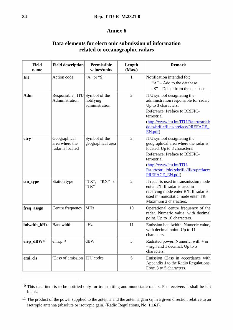
34 Rep. ITU-R M.2321-0

Annex 6

Data elements for electronic submission of information

related to oceanographic radars

Field

name

Field description Permissible

values/units

Length

(Max.)

Remark

Int Action code “A” or “S” 1 Notification intended for:

“A” – Add to the database

“S” – Delete from the database

Adm Responsible ITU

Administration

Symbol of the

notifying

administration

3 ITU symbol designating the

administration responsible for radar.

Up to 3 characters.

Reference: Preface to BRIFIC-

terrestrial

(http://www.itu.int/ITU-R/terrestrial/

docs/brific/files/preface/PREFACE_

EN.pdf)

ctry Geographical

area where the

radar is located

Symbol of the

geographical area

3 ITU symbol designating the

geographical area where the radar is

located. Up to 3 characters.

Reference: Preface to BRIFIC-

terrestrial

(http://www.itu.int/ITU-

R/terrestrial/docs/brific/files/preface/

PREFACE_EN.pdf)

stn_type Station type “TX”, “RX” or

“TR”

2 If radar is used in transmission mode

enter TX. If radar is used in

receiving mode enter RX. If radar is

used in monostatic mode enter TR.

Maximum 2 characters.

freq_assgn Centre frequency MHz 10 Operational centre frequency of the

radar. Numeric value, with decimal

point. Up to 10 characters.

bdwdth_kHz Bandwidth kHz 11 Emission bandwidth. Numeric value,

with decimal point. Up to 11

characters.

eirp_dBW10 e.i.r.p.11 dBW 5 Radiated power. Numeric, with + or

– sign and 1 decimal. Up to 5

characters.

emi_cls Class of emission ITU codes 5 Emission Class in accordance with

Appendix 1 to the Radio Regulations.

From 3 to 5 characters.

10 This data item is to be notified only for transmitting and monostatic radars. For receivers it shall be left

blank.

11 The product of the power supplied to the antenna and the antenna gain Gi in a given direction relative to an

isotropic antenna (absolute or isotropic gain) (Radio Regulations, No. 1.161).

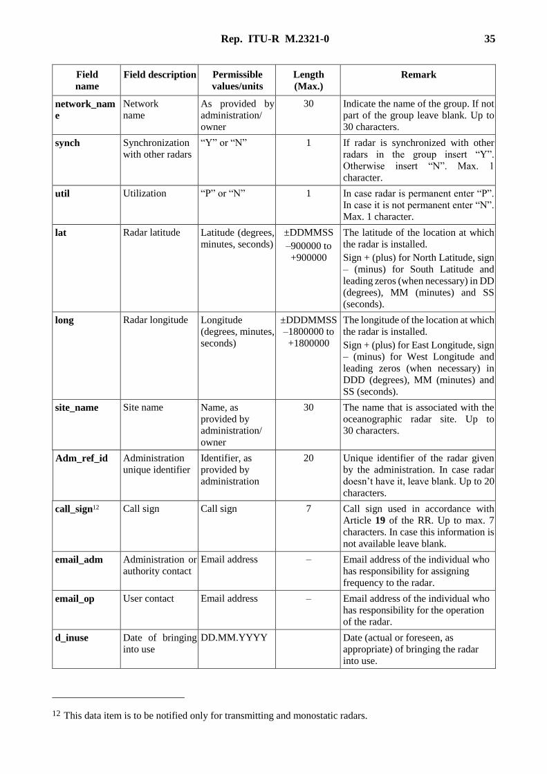
http://www.itu.int/ITU-R/terrestrial/docs/brific/files/preface/PREFACE_EN.pdf






Rep. ITU-R M.2321-0 35

Field

name


values/units

Length

(Max.)

Remark

network_nam

e

Network

name

As provided by

administration/

owner

30 Indicate the name of the group. If not

part of the group leave blank. Up to

30 characters.

synch Synchronization

with other radars

“Y” or “N” 1 If radar is synchronized with other

radars in the group insert “Y”.

Otherwise insert “N”. Max. 1

character.

util Utilization “P” or “N” 1 In case radar is permanent enter “P”.

In case it is not permanent enter “N”.

Max. 1 character.

lat Radar latitude Latitude (degrees,

minutes, seconds)

±DDMMSS

–900000 to

+900000

The latitude of the location at which

the radar is installed.

Sign + (plus) for North Latitude, sign

– (minus) for South Latitude and

leading zeros (when necessary) in DD

(degrees), MM (minutes) and SS

(seconds).

long Radar longitude Longitude

(degrees, minutes,

seconds)

±DDDMMSS

–1800000 to

+1800000

The longitude of the location at which

the radar is installed.

Sign + (plus) for East Longitude, sign

– (minus) for West Longitude and

leading zeros (when necessary) in

DDD (degrees), MM (minutes) and

SS (seconds).

site_name Site name Name, as

provided by

administration/

owner

30 The name that is associated with the

oceanographic radar site. Up to

30 characters.

Adm_ref_id Administration

unique identifier

Identifier, as

provided by

administration

20 Unique identifier of the radar given

by the administration. In case radar

doesn’t have it, leave blank. Up to 20

characters.

call_sign12 Call sign Call sign 7 Call sign used in accordance with

Article 19 of the RR. Up to max. 7

characters. In case this information is

not available leave blank.

email_adm Administration or

authority contact

Email address – Email address of the individual who

has responsibility for assigning

frequency to the radar.

email_op User contact Email address – Email address of the individual who

has responsibility for the operation

of the radar.

d_inuse Date of bringing

into use

DD.MM.YYYY Date (actual or foreseen, as

appropriate) of bringing the radar

into use.

12 This data item is to be notified only for transmitting and monostatic radars.

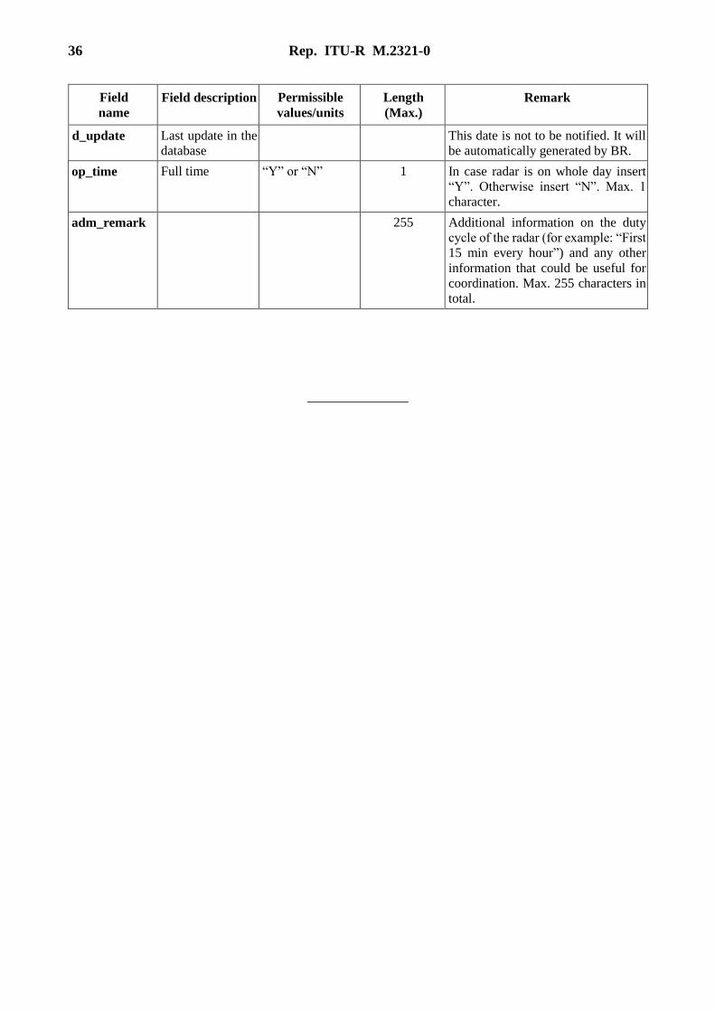
36 Rep. ITU-R M.2321-0

Field

name


values/units

Length

(Max.)

Remark

d_update Last update in the

database

This date is not to be notified. It will

be automatically generated by BR.

op_time Full time “Y” or “N” 1 In case radar is on whole day insert

“Y”. Otherwise insert “N”. Max. 1

character.

adm_remark 255 Additional information on the duty

cycle of the radar (for example: “First

15 min every hour”) and any other

information that could be useful for

coordination. Max. 255 characters in

total.

______________

Guidelines for the use of spectrum by oceanographic radars ... · oceanographic radars in the...

Documents

Transcript of Guidelines for the use of spectrum by oceanographic radars ... · oceanographic radars in the...