Kuo, Zeng, and Lord Paper No.: 12-3788

GUIDELINES FOR CHOOSING HOT-SPOT ANALYSIS TOOLS BASED ON DATA CHARACTERISTICS, NETWORK RESTRICTIONS, AND

TIME DISTRIBUSTIONS

Pei-Fen Kuo* Research Assistant

Zachry Department of Civil Engineering Texas A&M University

3136 TAMU College Station, TX 77843-3136 Email: p-kuo@ttimail.tamu.edu

Xiaosi Zeng

Research Assistant Zachry Department of Civil Engineering

Texas A&M University 3136 TAMU

College Station, TX 77843-3136 Email:

Dominique Lord

Associate Professor Zachry Department of Civil Engineering

Texas A&M University 3136 TAMU

College Station, TX 77843-3136 Tel. (979) 458-3949 Fax. (979) 845-6481

Email: d-lord@tamu.edu

*Corresponding Author November 14, 2011

Submitted for Presentation at the 91st Annual Meeting of the Transportation Research Board

Word Count: 4,925 + 2,500 (10 Figures) = 7,425 Words

Kuo, Zeng, and Lord

2

ABSTRACT A number of studies have shown different results in identifying crash hot-spots using different methods such as repeatability analysis, Moran I, Getis-Ord (Gi*), and Kernel Density Estimation (KDE). However, few researchers have discussed the reasons explaining the above differences; nor have they provided guidelines for selecting the most appropriate method for identifying hot-spots. Moreover, only a limited number of studies have analyzed crash data in conjunction with other types of data, such as those related to crime. In this research, a strategy is presented for choosing the most appropriate analysis tool to identify hot-spots that are consistent with the study’s limitations, data characteristics, and objectives. This study used crash and crime data provided by the College Station Police Department. Two important issues were addressed: (1) How to apply data characteristics to the problem of hot-spot identification (e.g., network restrictions for crashes, different hot-spot definitions for crimes and crashes); and, (2) How to incorporate spatial-time distributions in order to identify hot-spots. First, the solution was to apply network distance instead of straight-line distance as the point distance for any calculations, set a spatial limit of KDE, and combined KDE and Gi* maps to capture high risk areas and cluster patterns. Second, a spider graph was used to identify the temporal patterns of events occurring at different time scales: daily and weekly. Then, a co-map that combined a series of KDE maps according to the time of events was used to illustrate the spatial-temporal relationship of crash data to other events. The framework of this study can be used to identify high-risk areas for crash hot-spots and crime events.

Kuo, Zeng, and Lord

3

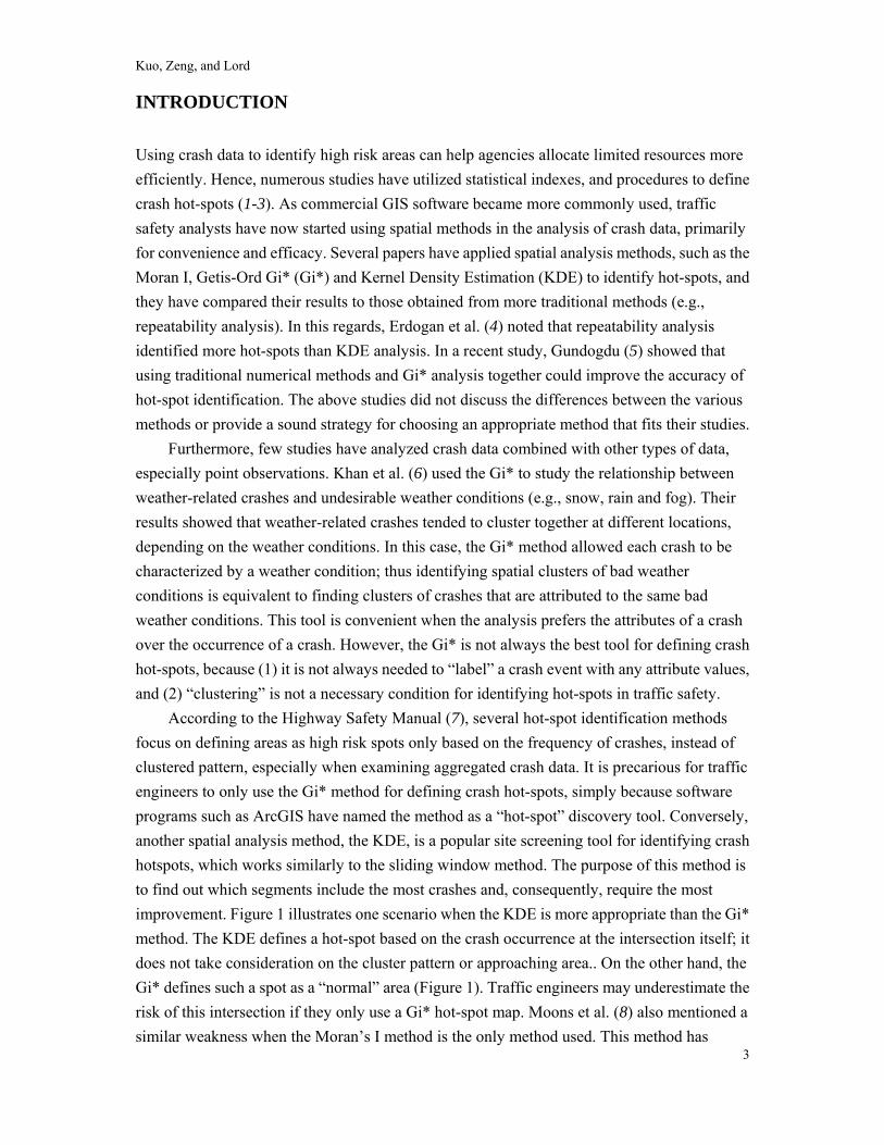
INTRODUCTION Using crash data to identify high risk areas can help agencies allocate limited resources more efficiently. Hence, numerous studies have utilized statistical indexes, and procedures to define crash hot-spots (1-3). As commercial GIS software became more commonly used, traffic safety analysts have now started using spatial methods in the analysis of crash data, primarily for convenience and efficacy. Several papers have applied spatial analysis methods, such as the Moran I, Getis-Ord Gi* (Gi*) and Kernel Density Estimation (KDE) to identify hot-spots, and they have compared their results to those obtained from more traditional methods (e.g., repeatability analysis). In this regards, Erdogan et al. (4) noted that repeatability analysis identified more hot-spots than KDE analysis. In a recent study, Gundogdu (5) showed that using traditional numerical methods and Gi* analysis together could improve the accuracy of hot-spot identification. The above studies did not discuss the differences between the various methods or provide a sound strategy for choosing an appropriate method that fits their studies.

Furthermore, few studies have analyzed crash data combined with other types of data, especially point observations. Khan et al. (6) used the Gi* to study the relationship between weather-related crashes and undesirable weather conditions (e.g., snow, rain and fog). Their results showed that weather-related crashes tended to cluster together at different locations, depending on the weather conditions. In this case, the Gi* method allowed each crash to be characterized by a weather condition; thus identifying spatial clusters of bad weather conditions is equivalent to finding clusters of crashes that are attributed to the same bad weather conditions. This tool is convenient when the analysis prefers the attributes of a crash over the occurrence of a crash. However, the Gi* is not always the best tool for defining crash hot-spots, because (1) it is not always needed to “label” a crash event with any attribute values, and (2) “clustering” is not a necessary condition for identifying hot-spots in traffic safety.

According to the Highway Safety Manual (7), several hot-spot identification methods focus on defining areas as high risk spots only based on the frequency of crashes, instead of clustered pattern, especially when examining aggregated crash data. It is precarious for traffic engineers to only use the Gi* method for defining crash hot-spots, simply because software programs such as ArcGIS have named the method as a “hot-spot” discovery tool. Conversely, another spatial analysis method, the KDE, is a popular site screening tool for identifying crash hotspots, which works similarly to the sliding window method. The purpose of this method is to find out which segments include the most crashes and, consequently, require the most improvement. Figure 1 illustrates one scenario when the KDE is more appropriate than the Gi* method. The KDE defines a hot-spot based on the crash occurrence at the intersection itself; it does not take consideration on the cluster pattern or approaching area.. On the other hand, the Gi* defines such a spot as a “normal” area (Figure 1). Traffic engineers may underestimate the risk of this intersection if they only use a Gi* hot-spot map. Moons et al. (8) also mentioned a similar weakness when the Moran’s I method is the only method used. This method has

Kuo, Zeng, and Lord

4

theoretical properties very close to that of the Gi*. In summary, a traffic engineer should first define “hot-spots” according to the contexts and goals of their safety analysis before applying GIS tools.

FIGURE 1 Different hot-spots defined by KDE and Gi* methods

Besides the different definitions of hot-spots, another challenge for identifying hot-spots related to crash data is the network restrictions. Crashes are limited to the road network, but other data (e.g., crimes) may happen anywhere, such as within a university campus building without any direct road access (or one on private property). Generally, there are two techniques for incorporating these network restrictions. The first one is to adjust the geographical weight matrix using network distances instead of 2-D planar distances. See Moons et al. (8) and Steenberghen et al.(9) for details regarding the updated Moran’s I and Gi* methods. The second technique is to set a spatial limit of KDE, with no KDE outside the boundary (10, 11). The above studies applied network restrictions with respect to Gi* and KDE, separately. This study applied either no restrictions or network restrictions to Gi* and KDE, simultaneously; thus illustrating the differences between the two techniques.

The third challenge is to identify hot-spots by considering the different time distributions of crash and other data. For example, crimes and crashes may happen in the same neighborhood, but there is often no causality between these two events (12). The temporal distribution of crimes may relate to the specific characteristics of criminals or victims’ daily activities, while crashes may relate to the characteristics of traffic flows or drivers such as the peak period or Driving While Intoxicated (DWI). Although several Data-Driven Approaches to Crime and Traffic Safety (DDACT) studies have shown the benefits of connecting hot-spots of crimes and crashes to aid in designing police patrol routes; how different time distributions affect the effectiveness of DDACT is still unclear. It would be over-simplistic to state that

Kuo, Zeng, and Lord

5

previous studies assumed that the time distributions of crimes and crashes were the same, which resulted in no recordable temporal effects.

After reviewing a number of related studies, this study focused on two important issues: (1) How to apply certain data characteristics to hot-spot identification (e.g., network restrictions for crash data, different hot-spot definitions for crimes and crashes), and (2) How to incorporate spatial-time distributions to locate hot-spots.

The next section explains the methodology and study data.

METHODS This study uses four methods: (1) Gi* and KDE without restriction, (2) Gi* and KDE with Network Restrictions, (3) Spider Graphs, and (4) Co-maps. The following paragraphs discuss the theoretical background and application of each method. Getis Ord Gi*and Kernel Density without Network Restrictions Numerous studies have shown the formula for Gi*and KDE as equations (1) and (2). The reasons why they are explained here are as follows:

• Example data are applied to equations (1) and (2) in order to demonstrate the different results they produce;

• Examples of the two methods serve as a basic foundation for the analysis that follows, which explains how to add network restrictions to these equations.

, ,1 1*

2 2, ,

1 1

( )

( )

1

n n

i j j i jj j

n n

i j i jj j

w D X X wGi

n w wS

n

= =

= =

−=

−

−

∑ ∑

∑ ∑ (1)

Where,

Gi*: The Getis Ord Gi* value for feature i; Wi,j(D): Weight between feature i and j D: The distance between feature i and j;

jX : The frequency at location j;

X : The average of crash frequency; S: Standard deviation of xj; and, n: The number of all features.

Kuo, Zeng, and Lord

6

22

2 2

3( ) (1 )d

dK iτ πτ τ<

= −∑ (2)

Where, K: Kernel density value; d: The distance from event; and, τ: Bandwidth.

Getis Ord Gi* and Kernel Density with Network Restrictions In this study, we used the same definition as Steenberghen et al. (9) to apply network restrictions. The distance in network restriction is called the “network distance,” while the straight-line distance is called the “planar distance”. Figure 2 illustrates the principal differences between the planar and network distances using two common scenarios: (1) when the center of measurement is on a freeway segment, and (2) when the center of measurement is near a complex highway interchange structure. As shown in Figure 2(a), it is easy to see that defining the neighborhood by using the planar distance may include any accidents occurring on the parallel frontage road. However, if the neighborhood can be defined within the network, as shown in Figure 2(b), accidents on the frontage road will not be “falsely” picked up. The situation is similar to those interchanges described in Figures 2(c) and (d).

FIGURE 2 Examples of Differences using Network and Planar Distances

R R

Point of Measurement

Accident Excluded

Accident Included

Coverage on the Network

Coverage on the Plane

Road Network

(a) Planar coverage on a freeway segment (c) Planar coverage on an interchange

(b) Network coverage on a freeway segment (d) Network coverage on an interchange

Kuo, Zeng, and Lord

7

Planar Kernel Density versus Network Kernel Density Generally, the KDE has a density at any location within the study region, while the network KDE has a density only on its network (10, 11). Instead of calculating the KDE density by area unit, the network KDE is estimated by liner unit. The density estimator of the network KDE (the Quartic function) is updated as:

22

2

3( ) (1 )d

dK uτ τ τ<

= −∑

(3)

The network KDE is very similar to the planar KDE, except that the normalizing constant

is τ instead of 2πτ . This is because the intensity of event i does not spread out over a unit area,

but rather only along the network links (see Figure 3). In general, 2πτ τ> unless 1τπ

< .

Therefore, each event may have a much stronger influence on their neighbors on the network rather than on a 2-D plane, given that the search radius τ stays constant. See Xie and Yan (11) and Sugihara et al. (10) for further details. This study used SANET (13) to calculate the network KDE.

(a) Planar KDE (b) Network KDE

FIGURE 3 Examples of Differences Using Planar KDE and Network KDE.

Kuo, Zeng, and Lord

8

Spider Graph An important question to ask when identifying hot-spots is “How long time-wise is a hot-spot ‘hot’?” (14); as a result, it is necessary to have access to an easy to use tool when identifying temporal hot-spots. Unlike a normal frequency figure which has time in the x-axis and frequency in the y-axis, a spider graph connects the beginning and the end times together, which results in the time axis acting as a circle. Its circular nature makes examining the complete time distribution much easier, because there is no interruption. Co-map Co-map is an extension of Co-plot. Co-plot uses point plots to show the effects of changing two variables; a co-map, however, uses a spatial distribution pattern map, much like KDE or a point density map (15). Co-map has been applied to several types of data, such as rainfall, fire, crime, and crashes (15-18) . After Plug et al. (19) integrated the use of a spider map into co-map, their results successfully demonstrated the spatial-temporal distribution of different types of crashes, just by the use of one figure, and without any animation or spatial modeling. Co-map is a useful exploratory tool for examining the spatial patterns of multivariate data, but other statistical models might be necessary for further analyses and predictions. However, Co-map is an excellent tool for showing the relationships between the crime and crash data collected for this study, because crime and crash data generally have no direct cause and effect relationships with each other. See Plug et al. (19) for additional details regarding the advantages and disadvantages of co-maps. The motivation behind combining crime and crash hot-spots when designing quality police patrol routes can be found in (20).

DATA AND STUDY AREA This study used the same observed data set as in (20) in order to compare the differences between hot-spots with and without network restrictions and time distributions. The study area is limited by the service area of the College Station Police Department (CSPD). Data were collected from January of 2005 to September of 2010. All crime and crash data were provided by the CSPD. There were 65,461 crime offense reports and 14,712 crash reports in total. The road shapefile, “All Line Data,” was downloaded from the Census Bureau's MAF/TIGER database website. The coordinate system used was the North America Datum 1983 (NAD83). The bandwidth was 2000 feet.

Kuo, Zeng, and Lord

9

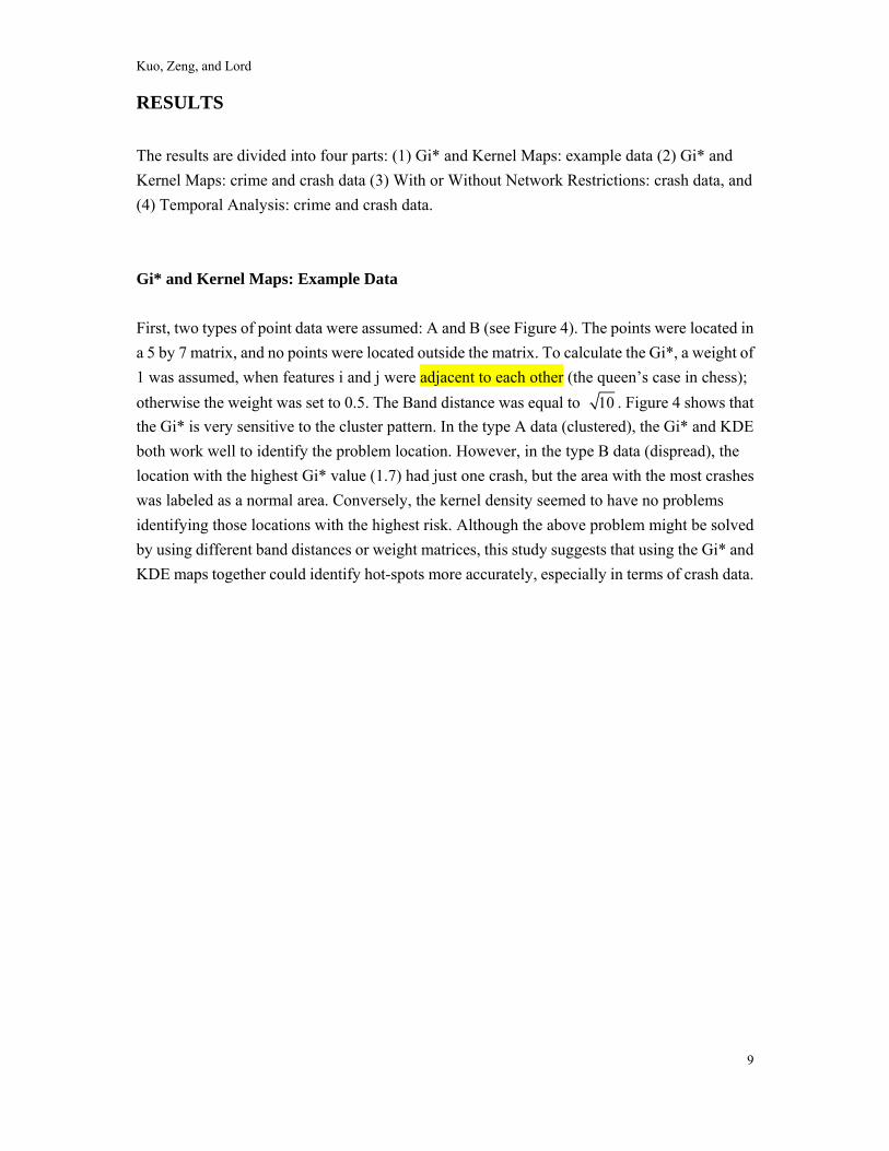
RESULTS The results are divided into four parts: (1) Gi* and Kernel Maps: example data (2) Gi* and Kernel Maps: crime and crash data (3) With or Without Network Restrictions: crash data, and (4) Temporal Analysis: crime and crash data. Gi* and Kernel Maps: Example Data First, two types of point data were assumed: A and B (see Figure 4). The points were located in a 5 by 7 matrix, and no points were located outside the matrix. To calculate the Gi*, a weight of 1 was assumed, when features i and j were adjacent to each other (the queen’s case in chess); otherwise the weight was set to 0.5. The Band distance was equal to 10 . Figure 4 shows that the Gi* is very sensitive to the cluster pattern. In the type A data (clustered), the Gi* and KDE both work well to identify the problem location. However, in the type B data (dispread), the location with the highest Gi* value (1.7) had just one crash, but the area with the most crashes was labeled as a normal area. Conversely, the kernel density seemed to have no problems identifying those locations with the highest risk. Although the above problem might be solved by using different band distances or weight matrices, this study suggests that using the Gi* and KDE maps together could identify hot-spots more accurately, especially in terms of crash data.

Kuo, Zeng, and Lord

10

FIGURE 4 Different Hot-spots Locations Found by Using the Gi* and Kernel Methods

Gi* and Kernel Maps without Network Restriction: Crime and Crash Data In Figure 5, the differences between the Gi* and KDE maps were compared for crime and crash data. At a glance, there seem to be no obvious differences between the crime-related hot-spots for the Gi* and KDE maps. However, for the crash data, the Gi* and KDE maps seem to identify different hot-spot areas. It is evident that the Gi* and KDE both show the largest hot-spots, all of which occur at the intersection with the highest traffic exposure in College Station, but they label different areas as secondary hot-spot areas. The Gi* shows secondary hot-spots on a highway segment located in the north, but the KDE shows secondary hot-spots in the Northgate area where bars and restaurants are concentrated. See circles in Figures (c) and (d). After zooming in on these two areas for a more detailed analysis, it is found that the Gi* map focused on clustered points, while the KDE map focused on points with extremely high values. These findings are consistent with the previous example.

Kuo, Zeng, and Lord

11

Crime

(a) Gi* (b) Kernel Crash

(c) Gi* (d) Kernel FIGURE5 Gi* and Kernel Maps of Crime and Crash Data without Network restrictions Gi* and Kernel Maps With Network Restriction: Crash Data Figure 6 includes the Gi* and the KDE maps for the crash data with network restrictions. Similar to the planar version comparison, the major hot-spots identified by both methods are comparable but they arrive at different locations for secondary hot-spots. From Figure 6-(a), one can notice that the Network Gi* identifies more hot-spots clustered close to the northern-most highway interchange and another hot-spot cluster in the western region of the city, as shown within the two red circles. On the other hand, the network KDE points out that the secondary hot-spots are still in the North-gate area where a mix of accidents locations with both high and low frequency counts, thus the Gi* method is insensitive in detecting it.

By comparing Figures 5 and 6, the hot-spot patterns are slightly different. Most differences are near major intersections and interchanges. This similarity is expected because the road network in College Station is rather simple; there were no complex interchanges in place during the period of analysis.

Kuo, Zeng, and Lord

12

However, there are fewer “hot-spots” and “cold-spots” in the network Gi*. Planar-based methods tend to over-detect crash hot-spots by capturing other hot-spots, while the network-based methods provide the crash hot-spot identification more accurately. This observation is consistent with findings elsewhere (11, 21). In highway accident analyses, network-based method should therefore be considered. Crash

(a) Gi* (b) KDE FIGURE 6 Gi* and Kernel maps of Crime and crash data with Network restrictions

Temporal Analysis According to spider graphs in Figure 7, the daily temporal patterns of crimes and crashes are very different. Crimes occurred fairly evenly from morning (8:00am) to late at night (02:00am), while crashes were most frequent during the afternoon rush hours (4:00pm to 6:00pm). For further analysis, crash and crime data were separated into two time periods (day and night) in order to draw KDE maps. Figure 7 shows the hot-spots for the crime and crash data, and how those hot-spots change from day to night. During the daytime, the hot-spots of crime were located in a local shopping mall and on the South Texas Avenue, while the hot-spots of crashes were located in one intersection that regularly experiences very heavy traffic (South Texas Avenue and Harvey Road). As for nighttime, the hot-spots of crimes and crashes were all located in the Northgate.

Kuo, Zeng, and Lord

13

Day (07:00-19:00) Night(19:00-7:00)

FIGURE 7 Co-map for comparison of Crimes and Crashes in College Station (daily)

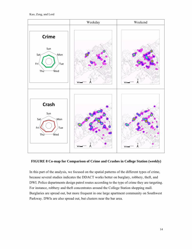
Figure 8 shows the weekly temporal patterns of crimes and crashes. Crimes occurred regularly and every day, while crashes were more frequent on Fridays and less often on Sunday. For further analyses, crash and crime data were separated into two time periods (weekday and weekend) for drawing KDE maps. Figure 8 shows how the hot-spots of crime change from weekday to weekend, but the hot-spots of crashes are almost the same for the weekdays and weekends. During the weekdays, most crimes happened in the bar area; however, during the weekend, most crime happened in the shopping mall and near South Texas Avenue. As for crashes, the hot-spots appeared along several main intersections and in the Northgate area.

12 3

456789

101112

131415

161718192021222324

Crime

12 3

456789

101112

131415

161718192021222324

Crash

Kuo, Zeng, and Lord

14

Weekday Weekend

FIGURE 8 Co-map for Comparison of Crime and Crashes in College Station (weekly)

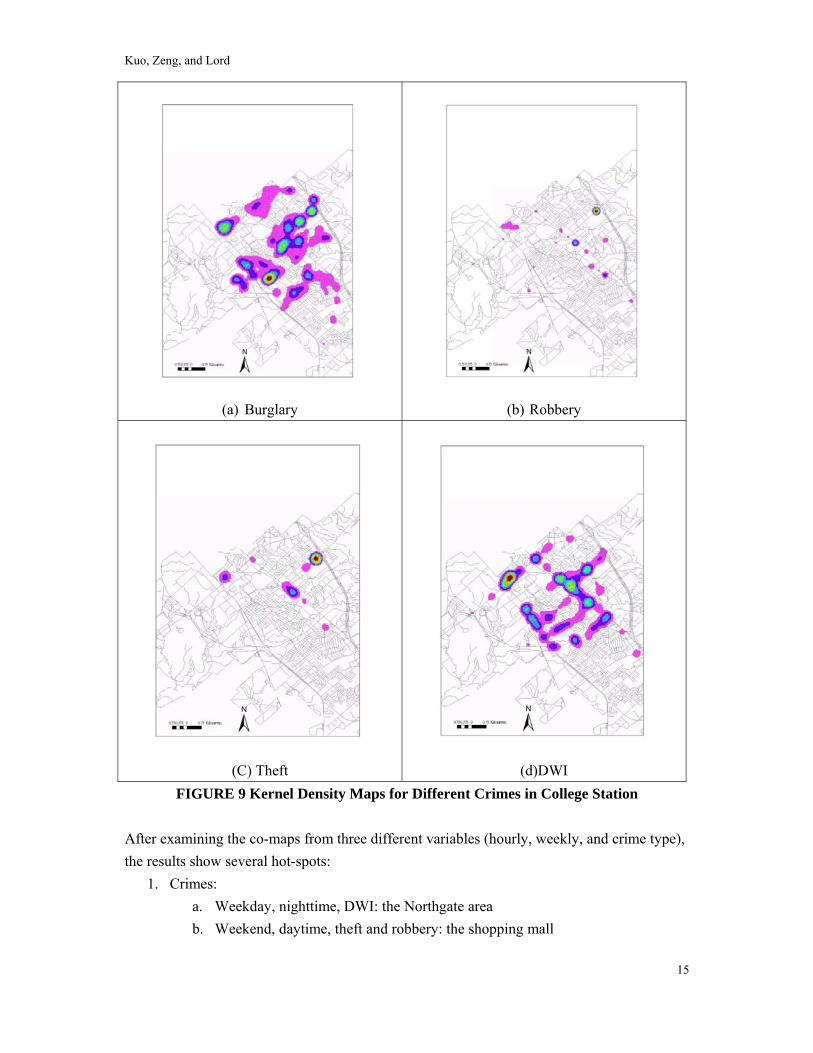
In this part of the analysis, we focused on the spatial patterns of the different types of crime, because several studies indicates the DDACT works better on burglary, robbery, theft, and DWI. Police departments design patrol routes according to the type of crime they are targeting. For instance, robbery and theft concentrates around the College Station shopping mall. Burglaries are spread out, but more frequent in one large apartment community on Southwest Parkway. DWIs are also spread out, but clusters near the bar area.

Sun

Mon

Tue

WedThu

Fri

Sat

Crime

Sun

Mon

Tue

WedThu

Fri

Sat

Crash

Kuo, Zeng, and Lord

15

(a) Burglary

(b) Robbery

(C) Theft

(d)DWI

FIGURE 9 Kernel Density Maps for Different Crimes in College Station After examining the co-maps from three different variables (hourly, weekly, and crime type), the results show several hot-spots:

1. Crimes: a. Weekday, nighttime, DWI: the Northgate area b. Weekend, daytime, theft and robbery: the shopping mall

Kuo, Zeng, and Lord

16

2. Crashes: a. Daytime (especially 4:00pm to 6:00pm): intersections with heavy traffic b. Nighttime (especially ~2:00am): the bar area

Using this type of mapping procedure, police departments can more easily organize their patrol routes using the above patterns, and target specific crimes. For example, focusing on the bar area during the weekdays and at night may be cost-effective, because this is clearly a temporal-spatial hot-spot. If the goal is to improve traffic safety, reducing the crime rate would be an extra bonus. Operating Route 1 and Route 2, as described in (20), would also work, because these Routes catch the hot-spots of crashes and crimes, such as DWI and robbery. However, if police departments want to reduce the rates of theft and robbery, increasing law enforcement in the shopping mall area during the weekend might be a better strategy. This study provides the framework for future law enforcement programs to organize their enforcement methods based on spatial-temporal hot-spots. The results of hourly and weekly analyses challenge the previous DDACT studies’ collective conclusion that the time distributions of crime and crashes are similar.

The findings described in this research advances the knowledge in identifying hotspots using different types of data. From this analysis, the following limitations of using Gi*, KDE maps, and co-maps were identified: 1. It may not be worthwhile to apply network restrictions to analyze crash data, especially in

places where most road networks are at the same elevations. In flat areas, a planar KDE would suffice.

2. Unlike KDE maps, the Gi* offers poor visual effects and cannot provide a clear boundary of risk. Take burglary and robbery data, for example. Using the KDE can define the region with the highest risk, including the region’s boundaries (Figure 9.a, 9.b). However, the Gi* only shows a large area covered in clusters illustrating a general high crime risk, and users cannot identify boundary line for high risk areas based on the point data (Figure 10.a,b).

3. The Gi* may have different definitions of the term “hot-spot” from those used by traffic safety professionals. Hot-spot in Gi* is defined as a point or area where incidents are clustered together by high values, but this is not necessarily a condition affecting traffic safety. Figure 10 (c) shows an area that KDE defines as a hot-spot while Gi* does not. The brown area includes several data points, but only one has an extremely high value. It is understandable why Gi* would show an area as normal that does not include a clustered pattern. However, traffic engineers could underestimate the risk in these areas, if they only use a Gi* map. A more cautious method of identifying hot-spots is to combine Gi* maps with other tools, such as the KDE maps.

4. The hot-spot results from using Gi* might be different, depending on the scale, location and aggregation units (19, 22).

5. The Gi* might have an unreliable Z-value for small or spread out data sets because of the limitations that come with a fixed distance band. A distance band should be large enough to

Kuo, Zeng, and Lord

17

ensure that all features have at least one neighbor, but the band should also not be so large that it lets in too many features. Also, for skewed data, the distance band should be large enough to ensure that several neighbors (for the best results, approximately eight) are included for each feature. In rural areas, crash rates tend to be very low (skewed right) and the locations are usually widely spread out. Hence, if one uses the GI* under these circumstances, the user is likely to receive a biased Z-value.

6. The hot-spots resulting from the KDE map are not statistically significantly, and different cell sizes and search bands may obviously affect the results. Researchers should be vigilant with the area of treatment, the study area, and the study scale.

7. Co-maps provide better visual effects, because a co-map combines several maps into one figure. This study recommends using KDE or 3D KDE maps to present spatial data instead of a Gi* map.

Kuo, Zeng, and Lord

18

(a) Burglary

(b) Robbery

FIGURE 10 (C) Differences between Kernel and Gi*

CONCLUSIONS AND FUTURE WORK Many studies have shown that using different methods of identifying crash hot-spots lead to different outcomes. Few researchers have tried to explain why such differences exist, nor have they provided appropriate guidelines for selecting appropriate methods of defining hot-spots. Moreover, few studies have analyzed crash data in conjunction with other types of data, such as those related to crime.

Kuo, Zeng, and Lord

19

This study presented a strategy for choosing the appropriate hot-spot analysis tool, that was dependent upon the study limitations, data characteristics, and the researchers’ interests or study objectives. Unlike prior research conducted by geographers and spatial statisticians, this research was designed by traffic engineers to solve real-life traffic problems. Two important issues were addressed in this study: (1) how to apply data characteristics to hot-spot identification (e.g., network restrictions for crash data, different hot-spot definitions for crime and crashes), and (2) how to incorporate spatial-time distributions in order to locate hot-spots. First, the study results have shown that the Gi* is very sensitive to the data cluster patterns, and combing KDE and Gi* maps can identify problem areas by overlaying high risk areas and cluster patterns. Hence, this technique provides a solution to the problem of using different definitions of hot-spots for crash and crime data. Second, this study used the network Gi* and network KDE methods, simultaneously. The results have shown that setting network restrictions does, indeed, separate some hot-spots that cluster at intersections or interchanges. This finding is not obvious from this particular study, since the road network in College Station is rather simple. Lastly, a spider graph and co-map were used to demonstrate the spatial-temporal interaction. Based on the co-maps of three different variables - hourly, weekly, and crime type - several hot-spots were identified, and the police department can now organize their patrol routes based on the above-mentioned hot-spots and the particular issues they seek to target. The results of hourly and weekly analyses challenge the DDACT assumption that the time distributions of crime and crashes are similar.

This study provides the framework for future research from screening networks, to identifying problem locations, to organizing responses based on spatial-temporal hot-spots. Future studies should compare the differences between using spatial analysis tools (i.e., Network KDE, Network Gi*) and Empirical Bayesian (EB) methods. Future work might also incorporate crash prediction models to identify those hot-spots with an unreasonably high crash risk.

REFERENCES 1. Geurts, K. and G. Wets. Black Spot Analysis Methods: Literature Review. Report,

Flemish Research Center for Traffic Safety, Belgium, 2003. 2. Hauer, E., J. Kononov, B. Allery and M. S. Griffith. Screening the Road Network for

Sites with Promise. In Transportation Research Record: Journal of the Transportation Research Board, No. 1784, Transportation Research Board of the National Academies, Washington, D.C., 2002, pp. 27-32.

3. Miranda-Moreno, L. F. Statistical Models and Methods for Identifying Hazardous Locations for Safety Improvements. PhD thesis, University of Waterloo, 2006.

4. Erdogan, E., I. Yilmaz, T. Baybura and M. Gullu. Geographical Information Systems Aided Traffic Accident Analysis System Case Study: City of Afyonkarahisar. Accident

Kuo, Zeng, and Lord

20

Analysis Prevention, Vol. 40, No. 1, 2008, pp. 174-181. 5. Gundogdu, I. B. Applying Linear Analysis Methods to GIS-supported Procedures for

Preventing Traffic Accidents: Case Study of Konya. Safety Science, Vol. 48, No. 6, 2010, pp. 763-769.

6. Khan, X. Q. and D. A. Noyce. Spatial Analysis of Weather Crash Patterns. ASCE Journal of Transportation Engineering Vol. 134, No. 5, 2008, pp. 191-202.

7. Highway Safety Manual, First Edition, American Association of State Highway and Transportation Officials 2010.

8. Moons, E., T. Brijs and G. Wets. Improving Moran’s Index to Identify Hot Spots in Traffic Safety. Geocomputation and Urban Planning, Vol. 176, 2009, pp. 117-132.

9. Steenberghen, T., K. Aerts and I. Thomas. Spatial Clustering of Events on a Network. Journal of Transport Geography, Vol. 18, No. 3, 2010, pp. 411-418.

10. Sugihara, K., T. Satoh and A. Okabe, in The 2010 International Symposium on Communications and Information Technologies, IEEE, Tokyo, Japan, 2010, pp. 827 - 832.

11. Xie, Z. and J. Yan. Kernel Density Estimation of Traffic Accidents in a Network Space. Computers, Environment, and Urban Systems, Vol. 35, No. 5, 2008, pp. 396-406.

12. Wilson, R. E. Place as the Focal Point: Developing a Theory for the DDACTS Model. Geography & Public Safety, Vol. 2, No. 3, 2010, pp. 3-4.

13. Okabe, A. and K.-i. Okunuki. SANET: A Spatial Analysis along Networks (Ver.4.0), http://sanet.csis.u-tokyo.ac.jp/sub_en/program.html, Accessed Jul, 15th.

14. Harries, K. Mapping Crime: Principle and Practice. Report, U.S. Department of Justice, https://www.ncjrs.gov/html/nij/mapping/pdf.html, Washington, DC, 1999.

15. Brunsdon, C. The Comap: Exploring Spatial Pattern via Conditional Distributions. . Computers, Environment and Urban Systems, Vol. 25, 2001, pp. 53-68.

16. Asgary, A., A. Ghaffari and J. Levy. Spatial and Temporal Analysis of Structural Fire Incidents and Their Causes: A Case of Toronto, Canada. Fire Safety Journal, Vol. 45, No. 1, 2010, pp. 44-57.

17. Brunsdon, C., J. Corcoran and G. Higgs. Visualizing Space and Time in Crime Patterns: A Comparison of Methods. Computers, Environment and Urban Systems, Vol. 31, No. 1, 2007, pp. 52-75.

18. Corcoran, J., G. Higgs, C. Brunsdon and A. Ware. The Use of Comaps to Explore the Spatial and Temporal Dynamics of Fire Incidents: A Case Study in South Wales, UK. The Professional Geographer, Vol. 59, No. 4, 2007, pp. 521-536.

19. Plug, C., J. C. Xia and C. Caulfield. Spatial and Temporal Visualisation Techniques for Crash Analysis. Accident Analysis & Prevention, In Press, Corrected Proof, 2011.

20. Kuo, P.-F., D. Lord and T. D. Walden, in 3rd International Conference on Road Safety and Simulation, Indianapolis, USA, 2011.

21. Yamada, I. and J.-C. Thill. Comparison of Planar and Network K-Functions in Traffic

Kuo, Zeng, and Lord

21

Accident Analysis. Journal of Transport Geography, Vol. 12, No. 2, 2003, pp. 149-158.

22. O’Sullivan, D. and D. J. Unwin. Geographic Information Analysis, John Wiley & Sons, Inc, Hoboken, New Jersey, 2010.