GST 105: Introduction to Remote Sensing Lab 6: Supervised ... · PDF fileThe development of...

GST 105: Introduction to Remote Sensing Lab 6: Supervised Classification

Objective – Perform a Supervised classification

Document Version: 2014-08-08 (Beta)

Copyright © National Information Security, Geospatial Technologies Consortium (NISGTC) The development of this document is funded by the Department of Labor (DOL) Trade Adjustment Assistance Community College and Career Training (TAACCCT) Grant No. TC-22525-11-60-A-48; The National Information Security, Geospatial Technologies Consortium (NISGTC) is an entity of Collin College of Texas, Bellevue College of Washington, Bunker Hill Community College of Massachusetts, Del Mar College of Texas, Moraine Valley Community College of Illinois, Rio Salado College of Arizona, and Salt Lake Community College of Utah. This work is licensed under the Creative Commons Attribution 3.0 Unported License. To view a copy of this license, visit http://creativecommons.org/licenses/by/3.0/ or send a letter to Creative Commons, 444 Castro Street, Suite 900, Mountain View, California, 94041, USA.

Author: Richard Smith, Ph.D. Texas A&M University – Corpus Christi

:

Lab 6:Supervised Classification

Contents 1 Introduction ................................................................................................................. 3 2 Objective: Perform an Image Rectification ................................................................ 3 3 How Best to Use Video Walk Through with this Lab ................................................ 4 Task 1 Define New GRASS Location ............................................................................. 4 Task 2 Import and Group Imagery, and Set Region ........................................................ 6 Task 3 Create Training Dataset ...................................................................................... 10 Task 4 Perform Supervised Classification ..................................................................... 18 Task 5 Reclassify Spectral Classes to Information Classes ........................................... 22 Task 6 Challenge: Perform a Second Class Supervised Classification ......................... 24 5 Conclusion ................................................................................................................ 25 6 Discussion Questions ................................................................................................ 25

8/23/2014 of 25


1 Introduction

The Supervised classification method is another of the two commonly used “traditional” image classification routines. This method (as well as the unsupervised method) is often used with medium (> 20m) and coarse (> 1km) resolution multispectral remotely sensed imagery. More commonly the unsupervised and supervised classification methods are used together to form a hybrid image classification process to categorize pixels into land cover or land use types. The primary difference between the unsupervised and the supervised methods is the supervised classification process requires a spectral signature file (sometimes referred to as the “training samples” or “training signatures”). Creating and evaluating spectral signatures were discussed in the lecture material. This lab will provide an opportunity for student learn how to create and evaluate spectral signatures that can be used in a supervised image classification. This lab includes the following tasks:

• Task 1 – Define New GRASS Location • Task 2 – Import and Group Imagery, and Set Region • Task 3 – Create Training Dataset • Task 4 – Perform Supervised Classification • Task 5 – Reclassify Spectral Classes to Information Classes • Task 6 – Challenge: Perform a Second Class Supervised Classification

2 Objective: Perform a Supervised Classification Students will be introduced to the supervised classification method. QGIS and GRASS Tools do not provide access to GRASS’s classification functions, therefore, in this lab, the student will learn how to classify an image using the GRASS GIS Graphical User Interface (GUI). The primary objectives of this lab are:

1. Create and Evaluate Spectral Signatures 2. Perform a Supervised Classification 3. Recode Spectral Classes to Information Classes

A simple classification scheme will be used for the lab:

• Water • Agriculture • Grassland • Forest • Urban

8/23/2014 of 25


3 How Best to Use Video Walk Through with this Lab To aid in your completion of this lab, each lab task has an associated video that demonstrates how to complete the task. The intent of these videos is to help you move forward if you become stuck on a step in a task, or you wish to visually see every step required to complete the tasks. We recommend that you do not watch the videos before you attempt the tasks. The reasoning for this is that while you are learning the software and searching for buttons, menus, etc…, you will better remember where these items are and, perhaps, discover other features along the way. With that being said, please use the videos in the way that will best facilitate your learning and successful completion of this lab. Task 1 Define New GRASS Location In this task, we will define a new GRASS Location and Mapset to serve as our working environment for the unsupervised classification. Let’s create the Location and Mapset.

1. The data for this lab is located at C:\GST 105\Lab 6 on the lab machine. Copy this data to a new working directory of your choosing.

2. Open GRASS 6.4.3 GUI. In Windows, this can be found at StartAll ProgramsQGIS ChugiakGRASS GIS 6.4.3GRASS 6.4.3 GUI

This will open the ‘Welcome to GRASS GIS’ window (shown in Figure 1) and possibly a command prompt. You can ignore the command prompt for this exercise. We will use this Welcome window to create our new location.

8/23/2014 of 25


Figure 1: Welcome to GRASS GIS Window

3. Click Browse button and navigate to the ‘Lab 6 Data’ folder that you extracted

to your hard drive. 4. Create a new folder named ‘grassdata’ in your lab directory and select the new

folder as the database. 5. Click ‘Location wizard’ button on the ‘Welcome to GRASS GIS’ window.

This will open the ‘Define new GRASS Location’ wizard. 6. Verify that the GIS Data Directory points to the lab directory. 7. Set the Project Location and Location Title both to ‘Sacramento’. 8. Press Next. 9. Select ‘Select EPSG code of spatial reference system’. 10. Click Next. 11. Search for EPSG code 3309. Select 3309 NAD27 / California Albers. (Shown

in Figure 2).

8/23/2014 of 25


Figure 2: Choose EPSG Code 3309

12. Click Next to set the CRS. The ‘Select datum transformation’ window will appear.

13. Choose ‘1: Used in whole nad27 region’ as the datum transformation. 14. Click OK to set the datum transformation. 15. Click Finish on the summary to return to the GRASS Welcome window.

a. Note: If you receive a dialog telling you to change the default GIS data directory, press OK to dismiss.

16. A dialog box named ‘Location <Sacramento> created’ will appear asking if we wish to set the default region extents and resolution now. Click No.

17. A dialog box named ‘Create new mapset’ will appear asking if we wish to create a new mapset. Enter ‘Classification’, then press OK to create the mapset.

You should now have the Sacramento and two Mapsets created in the GIS Database (shown in Figure 3). We can now start our GRASS GIS Project.

Figure 3: Sacramento Location and Two Mapsets

18. Select ‘Classification’ from the Accessible mapsets list then click ‘Start GRASS’ button. This will open the GRASS GUI.

Task 2 Import and Group Imagery, and Set Region In this task, we will import the raster file that we will perform a supervised classification on, and create an image group. This will prepare the imagery for input for classification.

1. Click FileImport Raster DataCommon formats import [r.in.gdal]. This will open the ‘Import raster data’ module window.

2. Set the following options (see Figure 4 for reference): a. Source Type: File b. Source settings

8/23/2014 of 25


i. Format: Erdas Imagine Images (.img) ii. File: <lab directory>\tm_sacsub.img

c. List of GDAL layers i. tm_sacsub.img: checked

d. Add imported layers into layer tree: unchecked

Figure 4: Import raster data Options to Import tm_sacsub.img

3. Click ‘Import’ button then click ‘Close’ button to close the dialog. 4. Select the Layer Manager window and select the ‘Command console’ tab if it is

not already selected (shown in Figure 5). The console displays the results of the import function.

8/23/2014 of 25


Figure 5: Results of Raster Import Module Tool

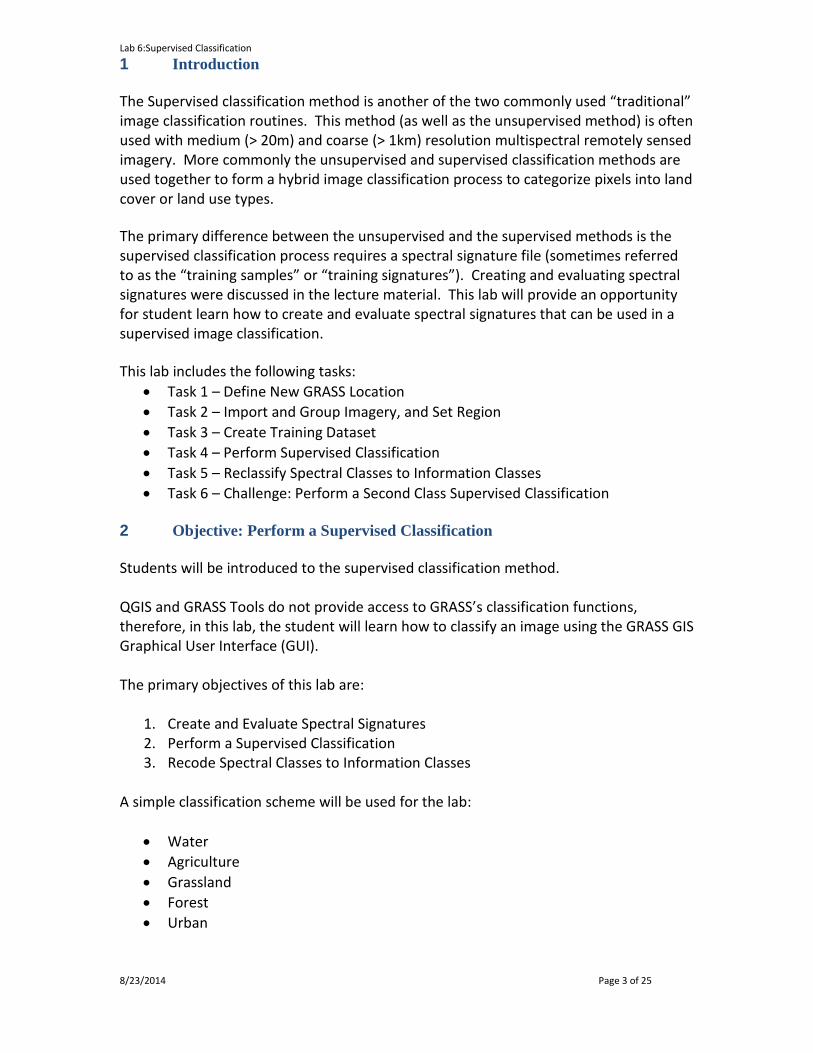
Note that the tool imported six rasters; one raster for each raster band. GRASS treats each band as a separate raster map. Each band can be visualized separately, or, if desired, a composite can be created, such as the composite created in Lab 3 for this course. To perform an image classification, the raster maps (bands) must be combined in to a group and subgroup. A group is a collection of raster maps. A subgroup is a subset of the group’s raster maps that will be utilized in the image classification. So, for instance, if you had a group of bands 1,2,3,4,5,6, but only wanted to use bands 3, and 4 for analysis, you would create a subgroup containing only bands 3 and 4. When we imported tm_sacsub, GRASS created a group for us named ‘tm_sacsub’. We will edit the group containing all 6 raster maps to add a subgroup containing all of the raster maps, since we will use all bands for our unsupervised classification.

5. Click ImageryDevelop images and groupsCreate/edit group [i.group]. This will open the ‘Create or edit imagery groups’ tool.

6. Enter ‘tm_sacsub_group’ as the group name in the top dropdown box. The ‘Layers in selected group’ should automatically populate with the six tm_sacsub raster maps (see Figure 6).

a. If the layers do not populate, click ‘Add’ and check the boxes next to the six tm_sacsub.n maps.

8/23/2014 of 25


Figure 6: Editing tm_sacsub Imagery Group

7. Check ‘Define also sub-group…’. 8. Click OK to add the sub-group and dismiss the tool.

Now that the imagery has been loaded, and a group and subgroup have been specified, the last step is to set the region. If you recall from Lab 3, a Region is a subset of a Location defined by a rectangular bounding box. The Region is important for raster and imagery operations as it bounds the area (region) that will participate in any raster and imagery operations executed in GRASS. A Region is an operating parameter set when working in GRASS. Let’s set the region equal to one of the tm_sacsub raster maps.

9. Click SettingsRegionSet region [region] on the Layer Manager window. This will open the region tool.

10. Set the following options: a. [multiple] Set region to match this raster map:

tm_sacsub.1@Classification i. Note: The ‘@Classification’ denotes that tm_sacsub.1 is stored in

the ‘Classification’ mapset. 11. Click ‘Run’. The tool will switch to the ‘Command output’ tab. If you do not see

any line that begins with the word ‘ERROR’, then the region has been successfully set.

12. Click ‘Close’ to close the region tool. With the imagery loaded, group and subgroup defined, and region set, we can now perform the unsupervised classification. 8/23/2014 of 25


Task 3 Create Training Dataset In this task, we will perform a supervised classification. There are two steps when performing a supervised classification: training, and classification. In the training step, a training dataset is created that classifies sample portions of the input imagery. This training dataset will then be passed to step two where it will be used when determining how to classify the image. You can think of it as the user (you) showing the computer a few examples of how you would like have the image classified, and then letting the computer rely on your examples to classify the rest of the image based on what it learned from you. For the first step, training, we will create a new vector map and digitize a few sample areas of the image and set the classes we wish to have similar areas classified as when the computer performs the supervised classification. Next, we will convert the vector map to a raster map which will then be pass to step two for use in classification. Let’s perform the training step now.

1. Click VectorDevelop vector mapCreate new vector map from the Layer Manager menu bar. This will open the ‘Create new vector map’ dialog.

2. Set the following options: a. Name: Training b. Create attribute table: checked

i. Key column: category c. Add created map into layer tree: checked

3. Click OK to create the Training vector map and add it to the layer tree. 4. In the layer tree, right-click on the Training vector map and choose ‘Show

attribute data’ from the contextual menu. This will open the ‘GRASS GIS Attribute Table Manager’ window which allows for display, query, and modification of the vector map’s attribute table.

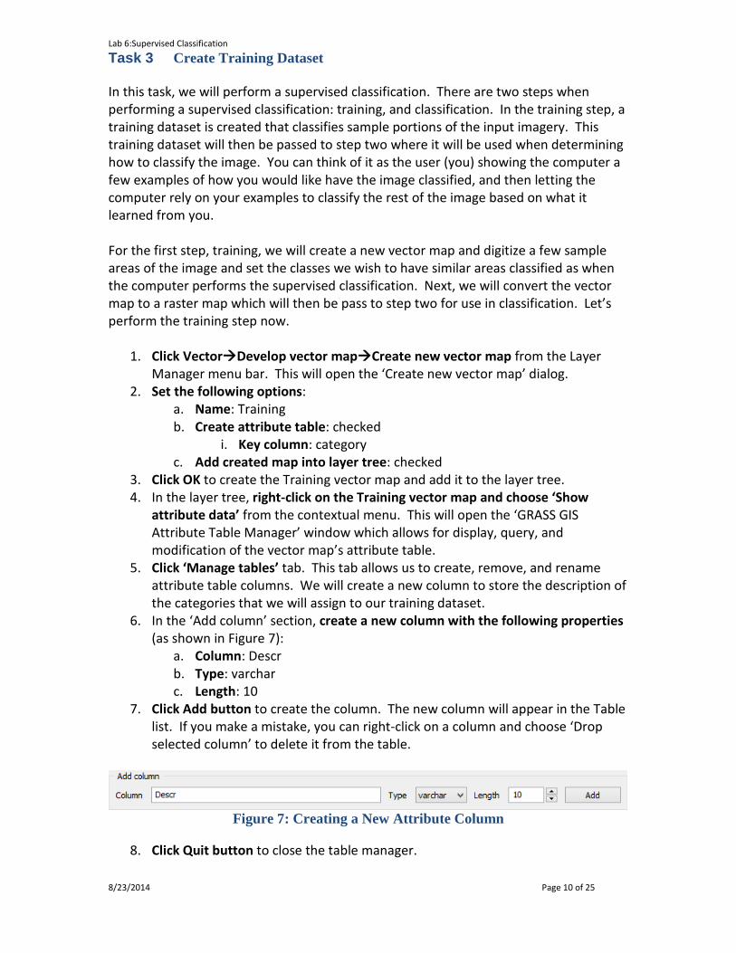
5. Click ‘Manage tables’ tab. This tab allows us to create, remove, and rename attribute table columns. We will create a new column to store the description of the categories that we will assign to our training dataset.

6. In the ‘Add column’ section, create a new column with the following properties (as shown in Figure 7):

a. Column: Descr b. Type: varchar c. Length: 10

7. Click Add button to create the column. The new column will appear in the Table list. If you make a mistake, you can right-click on a column and choose ‘Drop selected column’ to delete it from the table.

Figure 7: Creating a New Attribute Column

8. Click Quit button to close the table manager.

8/23/2014 of 25


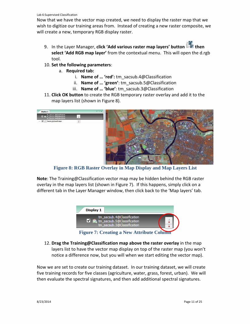
Now that we have the vector map created, we need to display the raster map that we wish to digitize our training areas from. Instead of creating a new raster composite, we will create a new, temporary RGB display raster.

9. In the Layer Manager, click ‘Add various raster map layers’ button then select ‘Add RGB map layer’ from the contextual menu. This will open the d.rgb tool.

10. Set the following parameters: a. Required tab:

i. Name of … ‘red’: tm_sacsub.4@Classification ii. Name of … ‘green’: tm_sacsub.5@Classification

iii. Name of … ‘blue’: tm_sacsub.3@Classification 11. Click OK button to create the RGB temporary raster overlay and add it to the

map layers list (shown in Figure 8).

Figure 8: RGB Raster Overlay in Map Display and Map Layers List

Note: The Training@Classification vector map may be hidden behind the RGB raster overlay in the map layers list (shown in Figure 7). If this happens, simply click on a different tab in the Layer Manager window, then click back to the ‘Map layers’ tab.

Figure 7: Creating a New Attribute Column

12. Drag the Training@Classification map above the raster overlay in the map layers list to have the vector map display on top of the raster map (you won’t notice a difference now, but you will when we start editing the vector map).

Now we are set to create our training dataset. In our training dataset, we will create five training records for five classes (agriculture, water, grass, forest, urban). We will then evaluate the spectral signatures, and then add additional spectral signatures.

8/23/2014 of 25


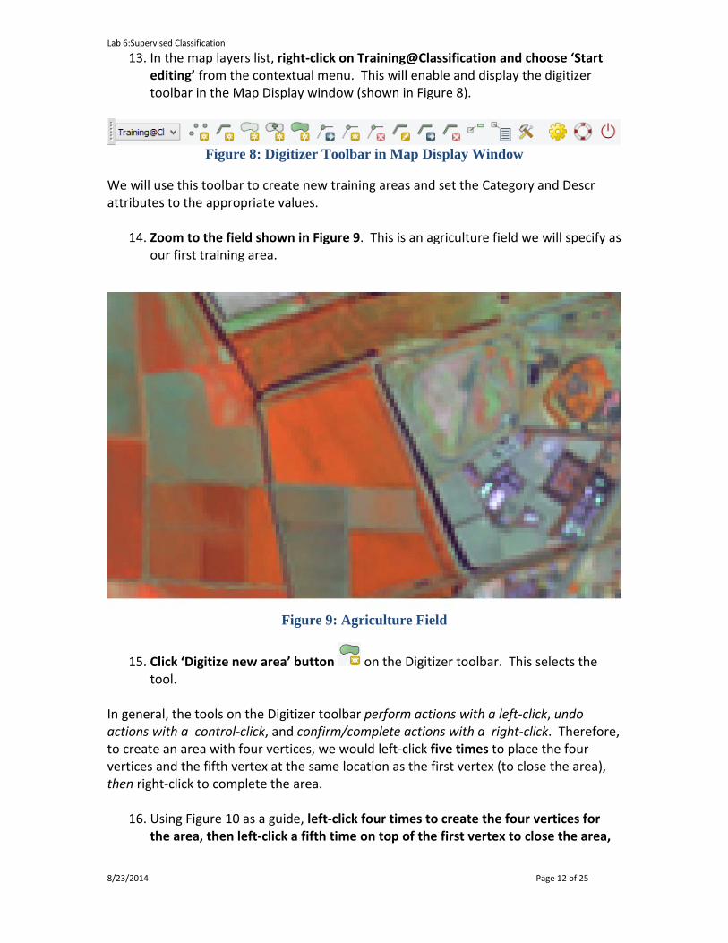
13. In the map layers list, right-click on Training@Classification and choose ‘Start editing’ from the contextual menu. This will enable and display the digitizer toolbar in the Map Display window (shown in Figure 8).

Figure 8: Digitizer Toolbar in Map Display Window

We will use this toolbar to create new training areas and set the Category and Descr attributes to the appropriate values.

14. Zoom to the field shown in Figure 9. This is an agriculture field we will specify as our first training area.

Figure 9: Agriculture Field

15. Click ‘Digitize new area’ button on the Digitizer toolbar. This selects the tool.

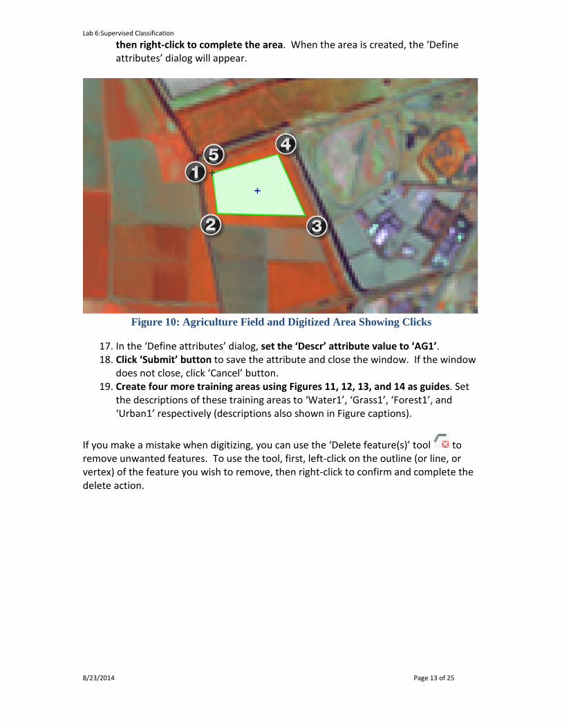
In general, the tools on the Digitizer toolbar perform actions with a left-click, undo actions with a control-click, and confirm/complete actions with a right-click. Therefore, to create an area with four vertices, we would left-click five times to place the four vertices and the fifth vertex at the same location as the first vertex (to close the area), then right-click to complete the area.

16. Using Figure 10 as a guide, left-click four times to create the four vertices for the area, then left-click a fifth time on top of the first vertex to close the area,

8/23/2014 of 25


then right-click to complete the area. When the area is created, the ‘Define attributes’ dialog will appear.

Figure 10: Agriculture Field and Digitized Area Showing Clicks

17. In the ‘Define attributes’ dialog, set the ‘Descr’ attribute value to ‘AG1’. 18. Click ‘Submit’ button to save the attribute and close the window. If the window

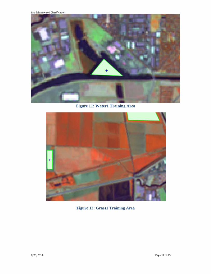
does not close, click ‘Cancel’ button. 19. Create four more training areas using Figures 11, 12, 13, and 14 as guides. Set

the descriptions of these training areas to ‘Water1’, ‘Grass1’, ‘Forest1’, and ‘Urban1’ respectively (descriptions also shown in Figure captions).

If you make a mistake when digitizing, you can use the ‘Delete feature(s)’ tool to remove unwanted features. To use the tool, first, left-click on the outline (or line, or vertex) of the feature you wish to remove, then right-click to confirm and complete the delete action.

8/23/2014 of 25


Figure 11: Water1 Training Area

Figure 12: Grass1 Training Area

8/23/2014 of 25


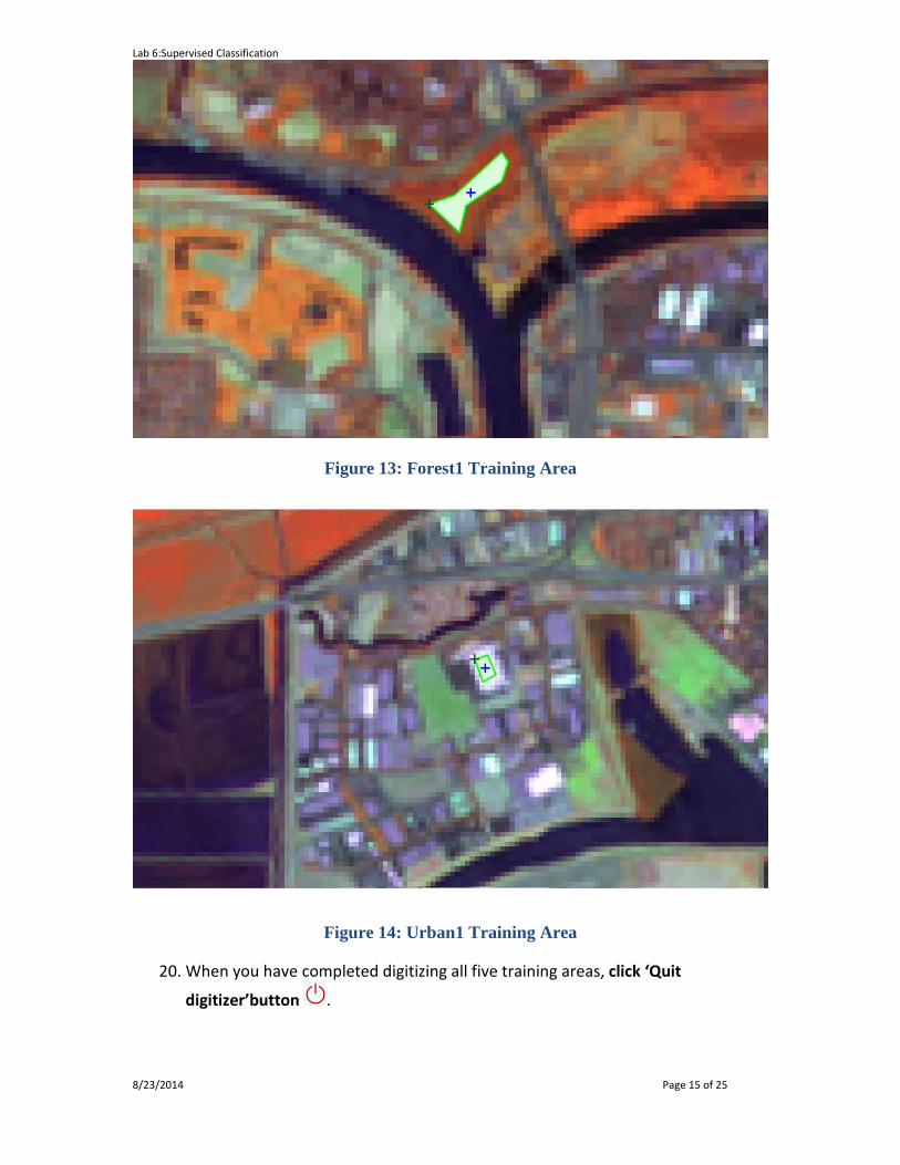
Figure 13: Forest1 Training Area

Figure 14: Urban1 Training Area

20. When you have completed digitizing all five training areas, click ‘Quit

digitizer’button .

8/23/2014 of 25


21. Click ‘Yes’ to the ‘Save changes?’ dialog to save your digitized training areas. The digitized areas will now display in a bland grey color letting you know that they have been saved to the vector map.

With the vector training map completed, the next step is to convert it to a raster map so it can be used for input into the first pass (i.gensig) of the supervised classification process.

22. Click VectorMap type conversionsVector to raster (v.to.rast) on the Layer Manager window. This will open the v.to.rast tool.


i. Name of input vector map: Training@Classification ii. Name for output raster map: TrainingAreas

iii. Source of raster values: attr b. Attributes tab:

i. Name of column for ‘attr’ parameter: category ii. Name of column...category labels: Descr

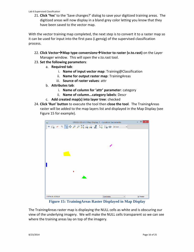
c. Add created map(s) into layer tree: checked 24. Click ‘Run’ button to execute the tool then close the tool. The TrainingAreas

raster will be added to the map layers list and displayed in the Map Display (see Figure 15 for example).

Figure 15: TrainingAreas Raster Displayed in Map Display

The TrainingAreas raster map is displaying the NULL cells as white and is obscuring our view of the underlying imagery. We will make the NULL cells transparent so we can see where the training areas lay on top of the imagery.

8/23/2014 of 25


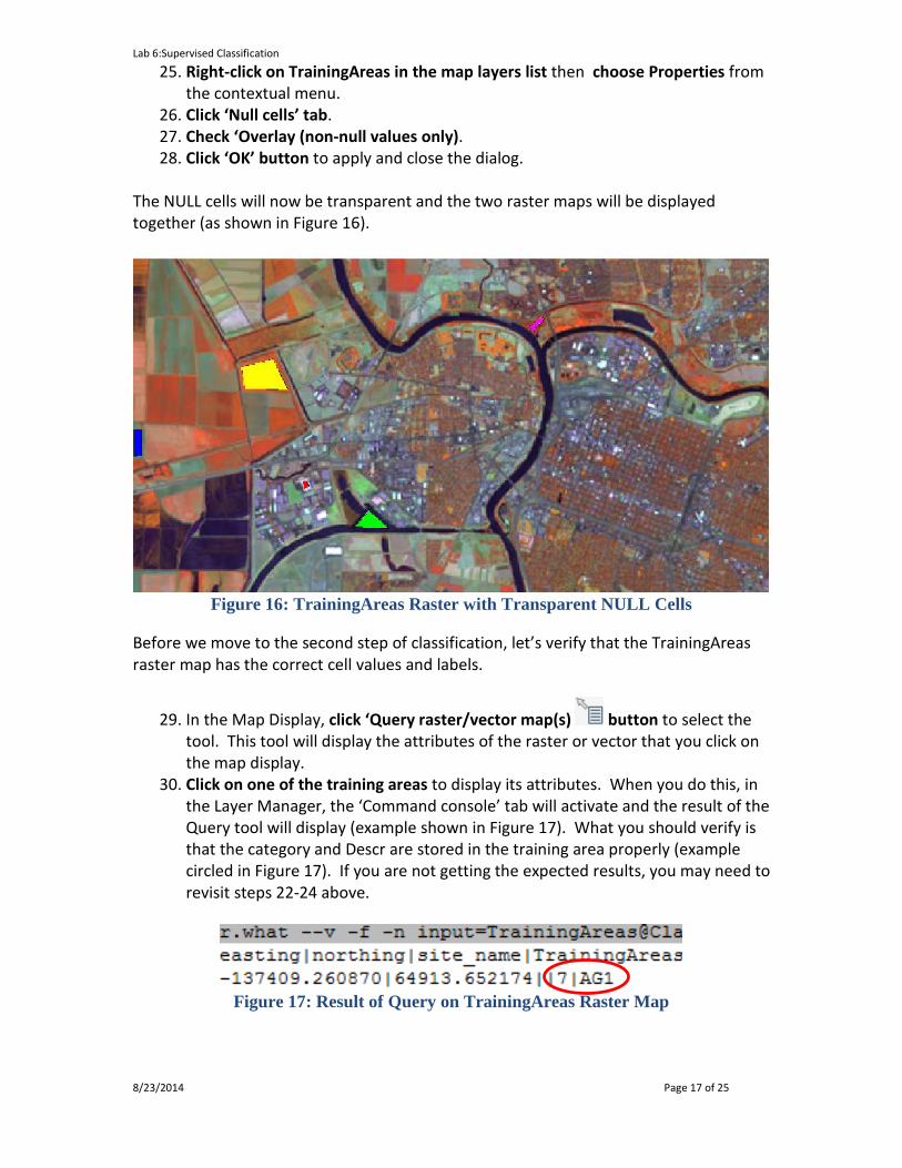
25. Right-click on TrainingAreas in the map layers list then choose Properties from the contextual menu.

26. Click ‘Null cells’ tab. 27. Check ‘Overlay (non-null values only). 28. Click ‘OK’ button to apply and close the dialog.

The NULL cells will now be transparent and the two raster maps will be displayed together (as shown in Figure 16).

Figure 16: TrainingAreas Raster with Transparent NULL Cells

Before we move to the second step of classification, let’s verify that the TrainingAreas raster map has the correct cell values and labels.

29. In the Map Display, click ‘Query raster/vector map(s) button to select the tool. This tool will display the attributes of the raster or vector that you click on the map display.

30. Click on one of the training areas to display its attributes. When you do this, in the Layer Manager, the ‘Command console’ tab will activate and the result of the Query tool will display (example shown in Figure 17). What you should verify is that the category and Descr are stored in the training area properly (example circled in Figure 17). If you are not getting the expected results, you may need to revisit steps 22-24 above.

Figure 17: Result of Query on TrainingAreas Raster Map

8/23/2014 of 25


Task 4 Perform Supervised Classification In this task, we will perform the second step of a supervised classification. In this step, we will first generate and review the spectral signatures of the training areas that we specified in the Task 3. Next, we will perform the supervised classification and review the results. Let’s start with generating the spectral signatures.

1. Click ImageryClassify imageInput for supervised MLC (i.gensig) on the Layer Manager window. This will open the i.gensig tool.

2. Read the manual for the i.gensig tool to learn what it does and what parameters it expects.

3. Set the following parameters for the i.gensig tool: a. Required tab:

i. Ground truth training map: TrainingAreas ii. Name of input imagery group: tm_sacsub_group

iii. Name of input imagery subgroup: tm_sacsub_group iv. Name for output file…: TrainingSignatures

4. Click ‘Run’ button to execute the tool. If no errors were reported, Close i.gensig dialog.

5. Open a text editor, such as Notepad and open <lab directory>\grassdata\ Sacramento\Classification\group\tm_sacsub_group\subgroup\ tm_sacsub_group\sig\TrainingSignatures. Tree structure shown in Figure 18.

Figure 18: Path to TrainingSignatures File

Let’s take a few moments to review and discuss the spectral signatures file partialy shown in Figure 19. Once the spectral signature is created, it can be evaluated to see if it looks like a high quality signature (that is, one that has a single bell-shaped histogram, and small standard deviations, and variances for each band).

8/23/2014 of 25


Figure 19: Portion of TrainingSignatures Spectral Signature File

The first line display the text label of the class, in this case, ‘AG1’ representing agriculture. The second line reports the number of cells in the class. The third line is the mean values per band of the class. The remaining lines are the semi-matrix of band-band covariance. Remember, the covariance matrix shows both the variance (the diagonal values shown in red in Figure 19) for a specific image band as well as how the spectral signature varies between different image bands (off-diagonal values). Ideally, each spectral signature will have a single ‘hump’, or peak value, on the diagonal, which tends to indicate a high quality spectral signature (as shown in Figure 19). If multiple ‘humps’ were returned, or the standard deviations and variances are very large, that would support the theory that the signature may be comprised of more than one land cover type.

6. Review the remaining classes in the spectral signature file. If any signatures seem to be a low quality signature, take note of them for discussion later.

Normally, you would re-create the training areas to gain a higher quality spectral signature, but for the purposes of learning, we will continue as you will be provided with a full set of training areas for the next few steps. A full set of training areas has been provided for you in the lab folder. We will import the vector training areas and convert them to a raster.

7. Click FileImport Vector DataCommon formats import [v.in.ogr]. This will open the ‘Import vector data’ module window.

8. Set the following options: a. Source Type: File b. Source settings

i. Format: ESRI Shapefile

Peak Value

8/23/2014 of 25


ii. File: <lab directory>\Spectral_Sigs_Training.shp c. List of GDAL layers

i. tm_sacsub.img: checked d. Add imported layers into layer tree: unchecked

9. Click ‘Import’ button then click ‘Close’ button to close the dialog. 10. Click VectorMap type conversionsVector to raster (v.to.rast) on the Layer

Manager window. This will open the v.to.rast tool. 11. Set the following parameters:

a. Required tab: i. Name of input vector map: Spectral_Sigs_Training@Classification

ii. Name for output raster map: TrainingAreas iii. Source of raster values: attr

b. Attributes tab: i. Name of column for ‘attr’ parameter: Classvalue

ii. Name of column...category labels: Classname c. Optional tab:

i. Allow output files to overwrite existing files: checked d. Add created map(s) into layer tree: checked

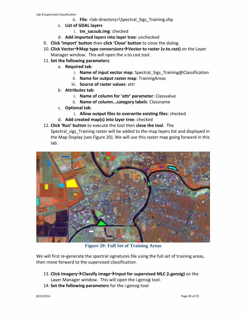
12. Click ‘Run’ button to execute the tool then close the tool. The Spectral_sigs_Training raster will be added to the map layers list and displayed in the Map Display (see Figure 20). We will use this raster map going forward in this lab.

Figure 20: Full Set of Training Areas

We will first re-generate the spectral signatures file using the full set of training areas, then move forward to the supervised classification.

13. Click ImageryClassify imageInput for supervised MLC (i.gensig) on the Layer Manager window. This will open the i.gensig tool.

14. Set the following parameters for the i.gensig tool: 8/23/2014 of 25


a. Required tab: i. Ground truth training map: Spectral_Sigs_Training@PERMANENT

ii. Name of input imagery group: tm_sacsub_group iii. Name of input imagery subgroup: tm_sacsub_group iv. Name for output file…: TrainingSignatures

15. Click ‘Run’ button to execute the tool. If no errors were reported, Close i.gensig dialog.

16. Review the newly created spectral signature file. Note that we now have 4 or 5 classes for each type of land cover.

With the spectral signature file review complete, we can now move on to the next step of the unsupervised classification: running the i.maxlik tool.

17. Click ImageryClassify ImageMaximum likelihood classification (MLC) [i.maxlik]. This will open the MLC tool.

18. Click the ‘Manual’ tab and read the manual for the MLC tool. When you are done reading the manual, proceed to the next step.

19. Click ‘Required’ tab and set the following options: a. Name of input imagery group: tm_sacsub_group@Classification b. Name of input imagery subgroup: tm_sacsub_group c. Name of file containing signatures: TrainingSignatures d. Name for raster map holding classification results: tm_sacsub_sup_class e. Add created map(s) into layer tree: checked

20. Click ‘Run’ to execute the MLC tool. 21. Check the Command output for errors. If none exist, click ‘Close’ to close the

MLC tool. 22. On the Layer Manager window, click Map layers. You should see our classified

image listed. On the Map Display, you should see the classified image (shown in Figure 21).

f. Note: if you do not see the image in the map display, right-click on the layer in the Map Layers list, and choose ‘Zoom to selected map(s)’ from the contextual menu.

8/23/2014 of 25


Figure 21: Supervised Classification Visualization

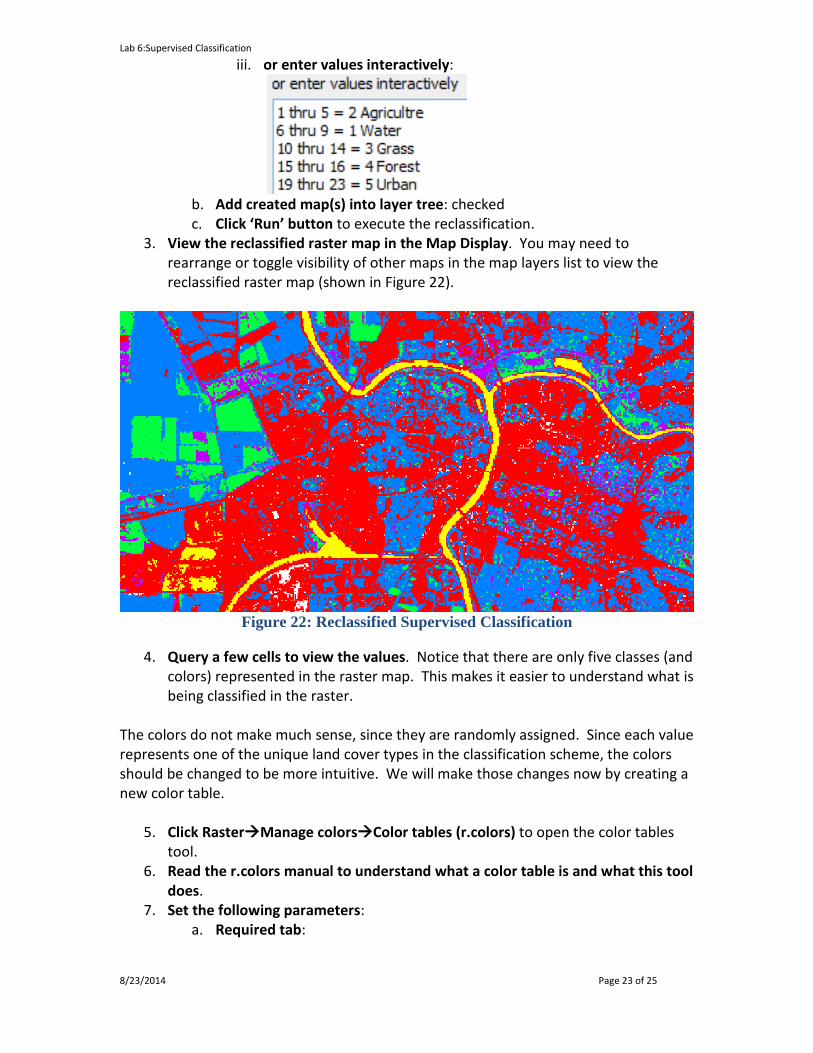
With the classification completed, we will now move to interpreting the result. Task 5 Reclassify Spectral Classes to Information Classes The final step in an image classification (and before an accuracy assessment is conducted) is to reclassify the spectral classes (that is the individual classes that represent the same land cover type to information classes (a single class for each unique land cover type). Recoding the spectral classes to information classes can be accomplished using the r.reclass tool. The following list can be used to reclassify existing spectral classes to information classes. Review the table, then let’s perfrom the reclassification. Spectral Class Number Information Class Number 1-5 2 - Agriculture 6-9 1 – Water 10-14 3 – Grass 15-16 4 – Forest 19-23 5 - Urban

1. Click RasterChange category values and labelsReclassify (r.reclass) to open the Reclassify tool.


i. Raster map to be reclassified: tm_sacsub_sup_clascs ii. Name for output raster map: tm_sacsub_sup_reclass

8/23/2014 of 25


iii. or enter values interactively:

b. Add created map(s) into layer tree: checked c. Click ‘Run’ button to execute the reclassification.

3. View the reclassified raster map in the Map Display. You may need to rearrange or toggle visibility of other maps in the map layers list to view the reclassified raster map (shown in Figure 22).

Figure 22: Reclassified Supervised Classification

4. Query a few cells to view the values. Notice that there are only five classes (and colors) represented in the raster map. This makes it easier to understand what is being classified in the raster.

The colors do not make much sense, since they are randomly assigned. Since each value represents one of the unique land cover types in the classification scheme, the colors should be changed to be more intuitive. We will make those changes now by creating a new color table.

5. Click RasterManage colorsColor tables (r.colors) to open the color tables tool.

6. Read the r.colors manual to understand what a color table is and what this tool does.


8/23/2014 of 25


i. Name of input raster map: tm_sacsub_sup_reclass b. Color tab:

i. or enter values interactively:

1. You can optionally save the color rules by clicking the ‘Save

As…’ button. These can later be loaded by clicking the ‘Load’ button.

8. Click ‘Run’ button to set the color table for the raster map. If no errors are displayed, close the Color tables dialog. You should now see the reclassified and recolored raster shown in Figure 23.

Figure 23: Recolored and Reclassified Supervised Classification

Task 6 Challenge: Perform a Second Class Supervised Classification Perform another supervised classification on the same data, however, this time, choose training areas you think would best represent the five land cover classes. Use as many training areas you see fit to get optimal results. Assign land cover classes in the same manner as above, perhaps combing a few classes together (if appropriate) using the r.reclass tool. Discuss the following:

1. Briefly describe your strategy in defining suitable training areas. 2. Compare your classified image to the classified image completed in Task 5. Were

you able to achieve a more accurate classified (based on your observations)? 8/23/2014 of 25


How and why did you deviate from what you did previously? Did your deviations improve or degrade the classification? Why/why not?

5 Conclusion This lab has introduced the primary steps to perform a supervised classification:

a. Creating and evaluate spectral signatures. b. The supervised classification method was implemented that uses the

spectral signature file. c. The Reclass and Color Table tools were used to convert spectral classes to

information classes. Students should have a good understanding of these steps and processes required to create a categorized image based on the supervised classification method. At the end of this lab, the final image classification is ready for an accuracy assessment. The accuracy assessment will be performed in Lab 7. 6 Discussion Questions

1. Submit your answers to the Task 6 questions. Include a picture of your classified image.

2. Describe the characteristics that define a ‘high quality’ spectral signature. 3. What is the purpose of performing a recode or reclassification? 4. In this lab, we digitized the training areas using GRASS GIS. This can also be done

in QGIS. List the steps required to digitize the training areas in QGIS and how you would import them into your GRASS Mapset.

8/23/2014 of 25

GST 105: Introduction to Remote Sensing Lab 6: Supervised ... · PDF fileThe development of...

Documents

Transcript of GST 105: Introduction to Remote Sensing Lab 6: Supervised ... · PDF fileThe development of...