Growth Options and Optimal Default under Liquidity

Constraints: The Role of Corporate Cash Balances

Attakrit Asvanunt Mark Broadie Suresh Sundaresan ∗

October 16, 2007

Abstract

In this paper, we develop a structural model that captures the interaction betweenthe cash balance and investment opportunities for a firm that has already some debtoutstanding. We consider a firm whose assets produce a stochastic cash flow stream.The firm has an opportunity to expand its operations, which we call a growth option.The exercise cost of the growth option can be financed either by cash or costly equityissuance. In absence of cash, we derive implicit solutions for equity and debt prices whenthe option is exercised optimally, under both firm value and equity value maximizationobjectives. We characterize the optimal exercise boundary of the option, and its impacton the optimal capital structure and the debt capacity of the firm. Next, we developa binomial lattice method to investigate the interaction between cash accumulationand the growth option. In this framework, the firm optimally balances the payout ofdividends with the buildup of a cash balance to finance the growth option in the “goodstates” (i.e., high asset value states), and to provide liquidity in the “bad states” (i.e.,low asset value states). We provide a complete characterization of the firm’s strategy interms of its investment and dividend policy. We find that while the ability to maintaina cash balance does not add significant value to the firm in absence of a growth option,it can be extremely valuable when a growth option is present. Finally, we demonstratehow our method can be extended to firms with multiple growth options.

Keywords: corporate policy, real options, binomial method

JEL Classification: C61, G12, G33

∗Asvanunt, aa2181@columbia.edu, Department of Industrial Engineering and Operations Re-search, Columbia University, New York, NY 10027; Broadie, mnb2@columbia.edu, and Sundaresan,ms122@columbia.edu, Graduate School of Business, Columbia University, New York, NY 10027. This workwas supported in part by NSF grant DMS-0410234, the JP Morgan Chase academic outreach program anda grant from the Moody’s Foundation.

1

1 Introduction

Management of cash plays a crucial role in the profitability and survival of companies. Early

literature on corporate debt valuation ignores the importance of cash by assuming that firms

can dilute equity at zero cost to finance coupon payments (e.g., Black and Cox (1976),

Leland (1994), Longstaff and Schwartz (1995), and Leland and Toft (1996)). Similarly,

standard literature on investment under uncertainty assumes that funds can be raised at

no cost to finance the investments (e.g., Brennan and Schwartz (1985) and McDonald and

Siegel (1986)). These models have been extended to address numerous issues, such as the

effects of strategic debt service, debt renegotiation, and U.S. bankruptcy provisions and

their effects on corporate debt valuation, and optimal financing and equity-bond holders’

conflict over timing of investments. While we provide a survey of this literature later in

the paper, it is important to note at the outset that there has been little work to address

important roles of cash and liquidity. In particular, we do not have coherent models of

corporate cash balances in a valuation setting, to help us understand the distinct roles

played by cash in good and bad states of the world, from a corporate perspective.

In this paper, we develop a structural model that captures two very essential roles of cash: i)

to provide liquidity during the time of financial distress, which may lead to bankruptcy and

costly liquidation, and ii) to finance future investment and growth opportunities. When

a firm is in a bad state (i.e., its asset value is low), its revenue may not be sufficient to

cover the coupon payments. In absence of cash, the firm will need to issue additional

equity, which may be costly, or declare bankruptcy. However, if the firm has accumulated

enough cash reserves, it can use it to postpone equity dilution and delay bankruptcy, or

even avoid them altogether if its asset value improves. On the other hand, when the firm

is in a good state (i.e., its asset value is high), it may wish to expand its operation by

investing in additional assets. The cost of raising capital in the future may be high (due

to informational asymmetry, for example), and it may be worthwhile to forego some of the

dividend distribution today to save up for future investments. The literature of seasoned

equity has documented that there are significant costs to issuing equity.1 Our framework1Corwin (2003) shows that seasoned equity offers were underpriced on average by 2.2% during the 1980s

2

allows us to characterize an optimal strategy for the firm regarding its dividend distribution,

cash holding, timing of investment and declaration of bankruptcy.

1.1 Literature Review

The real options approach to analyzing investment decisions under uncertainty was intro-

duced by Brennan and Schwartz (1985) and McDonald and Siegel (1986). They showed

that simple net present value analysis can lead to suboptimal decisions when projects are

irreversible. Dixit and Pindyck (1994) provide a good overview of the real options literature.

While many papers focus on the optimal time of an initial investment, our model considers

a firm that is already operational, and is looking for the optimal time to expand.

In the classical model of McDonald and Siegel (1986), the firm has an opportunity to invest

in a project whose value follows a geometric Brownian motion. They assume that the

investment decision is independent of the capital structure, and that the firm has unlimited

sources of funding to finance the project. More recent papers use the structural model

approach of Merton (1974) to evaluate growth options. The structural approach assumes

that the firm’s asset value follows a diffusion process, and the equity holders have a call

option on this asset. Mauer and Sarkar (2005) solve an investment problem in this setting,

as well as the optimal investment boundary and the optimal capital structure to finance

the project. In addition, they study the conflict between equity and debt holders, and

find that equity holders have a tendency to over-invest (compared to an investment policy

that maximizes the firm value), as they benefit from the up-side gain while the down-side

lost is shared by the debt holders. Titman and Tsyplakov (2006) further investigate this

conflict when the firm has the ability to adjust its capital structure dynamically. In a similar

setting, Sundaresan and Wang (2007b) consider an investment problem with strategic debt

service. Investment and financing distortions when there are multiple growth options are

investigated by Sundaresan and Wang (2007a).

Investment with liquidity constraints has been considered in several papers. Boyle and

Guthrie (2003) consider a firm with a cash reserve and existing assets whose market value

and 1990s, and that such discounts have increased substantially over time.

3

is constant. The existing assets produce a stochastic cash flow stream that contributes to

the growth of the cash reserve, in addition to the interest earned at a risk-free rate. The

firm must finance the investment internally, i.e., from the cash reserve and/or asset sales.

Hirth and Uhrig-Homburg (2006) consider a firm with a fixed amount of cash, equity and

debt outstanding, awaiting for the optimal time to invest in the production facility. During

the waiting period, the firm is not generating any revenue and is diluting equity to make

the coupon payments. Consequently, the firm may default even before the investment takes

place. If this happens, debt holders seize control, and the firm operates as if it were an

all-equity firm. They simultaneously solve for the optimal default and investment boundary.

In contrast to these models, our model considers a firm with a production facility already in

place, and is waiting to invest in another identical facility. In addition, instead of starting

with a fixed amount of cash (i.e., liquid assets), the firm in our model optimally distributes

dividends and accumulates cash from its revenue.

There are a few papers that model the cash reserve as a diffusion process instead of the asset

value. Jeanblanc-Picque and Shiryaev (1995) consider a cash process that follows standard

Brownian motion and solve for the optimal dividend policy as an optimal control problem.

Decamps and Villeneuve (2007) extend this model to incorporate a growth option, which

increases the drift of the cash process when exercised. Using a similar setting, Radner and

Shepp (1996) solve an investment problem where the firm has finitely many projects to

choose from.

1.2 Overview of Major Results

When maintaining a cash reserve is not permitted, we extend the result of Leland (1994) to

derive analytical solutions for equity and debt values of a firm with a growth option when

equity issuance is costly. Endogenous default and exercise boundaries are characterized by

a system of non-linear equations, which can be solved by standard numerical procedures.

In contrast to previous investment literature, we incorporate a cost of equity dilution in our

analysis. First, we show that the value of the growth option is increasing in both the equity

issuance cost and the asset’s volatility. While our result regarding volatility is consistent

4

with the investment literature (see Dixit and Pindyck (1994)), it is different from the results

of Decamps and Villeneuve (2007), where they find that volatility has ambiguous effects

on the value of a growth option. They discuss how an increase in the volatility can make

the option worthless in their model. Consistent with the results of Mauer and Ott (2000),

Titman and Tsyplakov (2006) and Moyen (2007), we find that equity value maximization

leads to a policy that exercises the option later (i.e., the exercise boundary is higher),

compared to a policy that maximizes the firm value. This is in contrast with the result

of Mauer and Sarkar (2005), where they find that an equity value maximizing policy leads

to exercising the option earlier. This is because in their setting, the cost of exercise is

partially financed through debt issuance. Our result shows that the difference between the

boundaries given by the two policies increases as the firm’s leverage increases. We also

find that having a growth option reduces the debt capacity and the leverage in the optimal

capital structure. This is consistent with the reported results in the literature.

In the second part of this paper, we develop a binomial method to determine equity and debt

values when the firm optimally distributes dividends and accumulates cash. In addition to

using it to pay for an exercise of a growth option, the firm also uses cash for coupon payments

whenever current revenue is not sufficient. Our method is robust, and can be easily extended

to accommodate different cost structures and multiple growth options. We solve for the

optimal strategy, and show that before the option is exercised, the firm’s strategy can be

completely characterized by three distinct regions, where the firm will either a) exercise the

option, b) not exercise and pay no dividend, or c) not exercise and pay dividends. After the

growth option is exercised, the strategy reduces to two regions where the firm either pays or

does not pay dividends. We find that the region where the firm neither exercises nor pays

dividends (case (b) above) is larger when the equity issuance cost or the liquidation cost

is higher. We show how the growth option and the ability to hold cash complement one

another. The benefit of one is greatly enhanced by the presence of the other, especially when

market frictions are significant. We investigate how the optimal levels of cash differ between

firms of different characteristics. Under firm value maximization, we find that the optimal

level is increasing with the riskiness of the firm, as measured by its default probability. This

5

result is consistent with empirical evidence that the correlation between the amount of cash

held in the firm and its credit spread is positive (e.g., Acharya et al. (2007)). We also study

the impact of a growth option and the firm’s leverage on its optimal cash level. Finally, we

extend our method to evaluate firms with multiple investment options.

The remainder of this paper is organized as follow. We introduce the general setup of the

model in Section 2, and provide the analysis of growth option without cash reserves in

Section 3. Cash reserves are included in the analysis in Section 4. Section 5 discusses the

extension of our results to multiple growth options, and Section 6 concludes the paper.

2 The Model

We assume that the firm’s asset value, denoted by Vt, is independent of its capital structure,

and follows a diffusion process whose evolution under the risk neutral measure Q is given

bydVtVt

= (r − q)dt+ σdWt,

where r is the risk-free rate, q is the instantaneous revenue rate, σ is the volatility of the

asset value, and Wt is a standard Brownian motion under Q.

The instantaneous revenue generated by the firm is given by

δt = qVt

At time zero, the firm issues debt with principal P , a continuous coupon rate C, and a

maturity T . There is a tax benefit of rate τ associated with coupon payments, such that

the effective coupon rate to the firm is (1 − τ)C. The firm uses its revenue δt to make

the coupon payment, and distribute the surplus as dividends to shareholders at the rate

dt ≤ δt− (1− τ)C. Any remaining revenue is accumulated in a cash reserve, whose current

balance is denoted by xt. The cash reserve is earning interest at a rate rx ≤ r, reflecting an

agency cost associated with leaving cash inside the firm.

6

Additionally, the firm has an option to increase its asset size by a factor g, at a fixed cost

K. In other words, exercising the option increases the asset value from Vt to (1 + g)Vt. At

the time of the exercise, if the firm has accumulated enough cash, i.e., if xt ≥ K, then it

uses cash to pay for the expansion. Otherwise, the firm issues additional equity to make

up the difference. We model frictions in the equity market by introducing a cost of equity

dilution, γ. Thus, when xt < K, the firm must issue (K − xt)/(1 − γ) dollars worth of

equity to exercise the option. The dilution cost, γ, does not only represent the physical

cost of issuing equity, such as underwriting and administrative fees, but other frictions in

equity issuance, such as agency and asymmetric informational cost as well. As noted by

Choe et al. (1993), the proportion of external financing by equity issuance is substantially

higher in expansionary phases. They suggest that the firms issue equity in such periods to

minimize the costs of adverse selection.

Finally, if the firm declares bankruptcy and liquidates its asset at time t, it incurs a liqui-

dation cost of αVt, leaving the debt holders with the remaining (1− α)Vt.

3 Welfare and Pricing in the Presence of a Growth Option

In this section, we provide analytical solutions for the equity and debt values, when the

firm is restricted from holding cash, and both the debt and the growth option have infinite

maturities.

Specifically, we restrict the dividend payout rate to be dt = (δt − C)+.2 We will assume

without loss of generality that τ = 0.3 We first derive closed-form solutions for equity and

debt values when bankruptcy and exercise boundaries are specified exogenously. In other

words, we assume that there is a lower boundary on the asset value VB, below which the

firm declares bankruptcy, and an upper boundary VG, above which the firm exercises the

growth option. Upon bankruptcy, the firm liquidates its asset and incurs a liquidation cost

of α, i.e., the proceeds from the liquidation are (1− α)VB.2The + operator is defined such that y+ = max(y, 0).3This assumption is just for expositional convenience. The role of debt is dependent on the existence of

corporate tax benefits in our model.

7

It is well known (e.g., Duffie (1988)) that for any security whose payoff depends on the asset

value Vt, its value f(Vt, t), must satisfy the following PDE:

12σ2V 2

t fV V + (r − q)VtfV − rf + ft + g(Vt, t) = 0 (1)

where g(Vt, t) is the payout received by the holders of this security.

In the perpetuity case, the security value becomes time-independent, and hence the previous

PDE reduces to the ODE:

12σ2V 2fV V + (r − q)V fV − rf + g(V ) = 0 (2)

Equation (2) has the general solution

f(V ) = A0 +A1V +A2V−Y +A3V

−X , (3)

where

X =

(r − q − σ2

2

)+

√(r − q − σ2

2

)2+ 2σ2r

σ2(4)

Y =

(r − q − σ2

2

)−√(

r − q − σ2

2

)2+ 2σ2r

σ2(5)

3.1 Equity Value

Consider a firm that issues perpetual debt, with a continuous coupon paid at the rate

C. When the firm’s revenue rate exceeds the coupon rate, i.e., qV ≥ C, equity holders

receive dividends at the rate qV −C. Otherwise the firm dilutes equity to make the coupon

payment, which is equivalent to receiving negative dividends at the rate β(qV −C), where

β = 1/(1− γ).

Let VG denote the exercise boundary of the growth option. Therefore, the equity value, E,

8

prior to exercising the option must satisfy:

12σ2V 2EV V + (r − q)V EV − rE + β(qV − C) = 0 for VB ≤ V ≤ C/q (6)

12σ2V 2EV V + (r − q)V EV − rE + qV − C = 0 for C/q ≤ V ≤ VG, (7)

together with the boundary, continuity and smooth pasting conditions:

(BC I): E(VB) = 0

(CC): E((C/q)−) = E(C/q)

(SP): EV ((C/q)−) = EV (C/q)

(BC II): E(VG) = E0((1 + g)VG)− βK,

(8)

where E0(V ) is the equity value under costly equity dilution in absence of the growth option,

as given in Asvanunt, Broadie, and Sundaresan (2007).

(BC I) follows from the assumption that shareholders get nothing when the firm declares

bankruptcy. (CC) and (SP) ensure that the equity value at the equity dilution boundary is

continuous and smooth. (BC II) follows from the fact that at the time of the exercise, the

firm’s asset value increases from V to (1+g)V , and since the firm only has one growth option,

its equity value must be the same as that of a firm without a growth option, evaluated at

(1+g)VG, less the cost of exercise βK. The expression for the equity value and its derivation

can be found in Appendix A.

3.2 Debt Value

Debt holders receive a constant payout rate of C as long as the firm remains solvent, i.e.,

while V ≥ VB. Therefore the debt value, D, must satisfy:

12σ2V 2DV V + (r − q)V DV − rD + C = 0 for V ≥ VB (9)

9

Equation (9) has a general solution:

D(V ) = B0 +B1V +B2V−Y +B3V

−X , (10)

where X and Y are given by (4) and (5).

Similar to solving for the equity value, we use the fact that D(V ) must satisfy the following

boundary conditions:

(BC I): D(VB) = (1− α)VB

(BC II): D(VG) = D0((1 + g)VG),(11)

where D0(V ) is the debt value under costly equity dilution in absence of the growth option

as given in Asvanunt, Broadie, and Sundaresan (2007).

(BC I) follows from the assumption on bankruptcy cost. (BC II) is the debt value when

the growth option is exercised. The debt value must be the same as that of a firm without

a growth option, evaluated at (1 + g)VG. The cost of the exercise is fully funded by equity,

hence there is no cost to the debt holders. The expression for the debt value and its

derivation can be found in Appendix A.

3.3 Endogenous Default and Exercise Boundaries

When the bankruptcy and the exercise of a growth option are determined endogenously by

the firm, we consider the two cases where the firm is maximizing the total firm value and

the equity value.

First we can determine the optimal bankruptcy boundary after the growth option is exer-

cised by numerically solving ∂v0

∂V

∣∣∣V=V 0

B

= 0 or ∂E0

∂V

∣∣∣V=V 0

B

= 0 for firm value maximization

or equity value maximization, respectively.

Prior to exercising the growth option, the optimal bankruptcy and exercise boundaries are

determined by similar smooth pasting conditions.

10

For firm value maximization, the optimal bankruptcy and exercise boundaries must satisfy:

∂v

∂V

∣∣∣∣V=VB

= 0 (12)

∂v

∂V

∣∣∣∣V=VG

=∂vL∂V

∣∣∣∣V=(1+g)VG

, (13)

where v(V ) = E(V ) +D(V ) is the total firm value.

Similarly, for equity value maximization, the boundaries must satisfy:

∂E

∂V

∣∣∣∣V=VB

= 0 (14)

∂E

∂V

∣∣∣∣V=VG

=∂EL∂V

∣∣∣∣V=(1+g)VG

(15)

We will sometimes refer to the result of firm value maximization as “first-best,” that of

equity value maximization as “second-best.” See Leland (1994) for a discussion of the

smooth pasting conditions.

The results presented in Sections 3.4 – 3.5 are computed as follows. First, we simultaneously

solve the smooth pasting conditions, (12) – (13) or (14) – (15), for the optimal boundaries,

VB and VG, numerically. Then, we use these boundaries in the closed-form solutions derived

in this section.

3.4 Optimal Exercise Boundary

In this section, we examine how the optimal exercise boundary changes with various model

parameters. We also look at the difference between the first-best and second-best policy.

Figure 1 plots the optimal exercise boundary for the growth option as a function of γ and

σ. We observe that the level of asset value above which the firm exercises the option is

increasing in both γ and σ. An increase in equity dilution cost effectively increases the cost

of exercising the option. Therefore, the firm would require a higher payoff from the option

when γ is higher. As a result, firms with higher equity dilution cost tend to wait longer

before they exercise. Volatility of the asset value impacts the riskiness of the firm. Since

11

the growth option in our model is an expansion of the existing operation, the riskier the

firm is, the riskier the new project is as well. It is well known from the standard growth

option literature (see, e.g., Dixit and Pindyck (1994)) that the value of the investment

increases with the project’s volatility, due to its upside potential. For the very same reason,

the firm will wait for the asset value to reach a higher level before exercising the option.

Consequently, we observe that the exercise boundary is increasing in σ.

0 0.05 0.1 0.15 0.2 0.25 0.3200

300

400

!

Firm

Max

VX*

Optimal Exercise Boundary versus Dilution Cost

0 0.05 0.1 0.15 0.2 0.25 0.30.5

1

1.5

Equi

ty M

ax V

X* (as

% in

crea

se o

ver F

irm M

ax)

Firm Max.Equity Max.

0.3 0.35 0.4 0.45 0.5 0.55 0.6400

600

800

1000

!

Firm

Max

VX*

Optimal Exercise Boundary versus Asset Volatility

0.3 0.35 0.4 0.45 0.5 0.55 0.62

2.2

2.4

2.6

Equi

ty M

ax V

X* (as

% in

crea

se o

ver F

irm M

ax)Firm Max.

Equity Max.

Figure 1: The left panel plots the optimal exercise boundary under first-best policy against equity dilutioncost, γ, when the firm has no cash balance. The boundary is increasing with γ. The right panel plotsit against the asset volatility, σ. The optimal boundary is also increasing with σ. Both panels also plotthe percentage change in exercise boundary if the firm follows second-best policy instead. In all cases, theboundary under first-best policy is always lower than under second-best policy. (V = 100, σ = 0.2, q =0.03, r = 0.05, C = 3, α = 0.3, τ = 0.15, γ = 0.15, g = 1, K = 100)

Figure 2 plots the exercise boundary versus the firm’s leverage. We define leverage as a

ratio of debt to total firm value. The left panel of Figure 2 shows that the asset value

exercise boundary is decreasing with leverage under the first-best policy, but is increasing

in leverage under the second-best policy. As the firm’s leverage increases, the equity value

decreases significantly. Hence, the boundary for an equity value maximizing firm needs to

be higher to compensate for the decrease in equity value. At the same time, an increase

in leverage has a relatively small impact on the total firm value. Therefore, the boundary

under firm value maximization decreases with leverage, as the default probability increases.

The right panel of Figure 2 shows that boundary on equity value is decreasing with leverage

under both policies.

In all of the cases discussed above, we find that the exercise boundary under the first-best

12

0 0.2 0.4 0.6 0.8 1240

250

260

270

280

290

300

Leverage

V X*

Optimal Exercise Boundary (Asset Value) versus Leverage

Firm Max.Equity Max.

0 0.2 0.4 0.6 0.8 1200

250

300

350

400

450

Leverage

E X*

Optimal Exercise Boundary (Equity Value) versus Leverage

Firm Max.Equity Max.

Figure 2: The left panel plots the optimal exercise boundary on asset value against leverage. The boundaryis decreasing with leverage under the first-best policy, but is increasing under the second-best policy. Theright panel plots the optimal exercise boundary on equity value. The optimal boundary in terms of the equityvalue is decreasing under both policies. The boundary is always lower for first-best policy than second-best.(V = 100, σ = 0.2, q = 0.03, r = 0.05, α = 0.3, τ = 0.15, γ = 0.15, g = 1, K = 100)

policy is always lower than that under the second-best policy. This means that the exercise

will occur later under the equity value maximization compared to firm value maximization.

The gap between the boundaries of the first-best and the second-best policy is small for firms

with low leverage, and rapidly increases as leverage increases. The driving factor behind

this result is the fact that the entire cost of investment is financed by the shareholders,

while the benefits are shared with the debt holders as well. As a result, an equity value

maximizing firm will demand a higher return from the investment.

3.5 Value of the Growth Option and its Impact on Capital Structure

In this section, we first look at how the value of the growth option varies across firms with

different characteristics, and its impact on optimal capital structure. The results under

the first-best and the second-best policy are very similar, so we will only discuss the results

under the first-best policy. The value of the growth option is the difference between the firm

(or equity) value, with and without the option. The left panel of Figure 3 plots the value

of the growth option against the equity dilution cost. As the equity dilution cost increases,

the option effectively becomes more expensive and hence we find that its value is decreasing

in γ. The right panel of Figure 3 plots the value of the growth option against the firm’s

13

asset volatility. As mentioned in Section 3.4, the value of the option is increasing in the

volatility of the project. We also find that under both first- and second-best policies, most

of the benefit of the growth option goes to the shareholders. Benefit to the debt holders

becomes larger as the volatility increases and the firm becomes riskier. This is because the

option reduces the probability of default and the dead-weight loss upon liquidation, which

is more prominent for riskier firms.

0 0.1 0.2 0.3 0.4 0.522

24

26

28

30

32

34

36Growth Option Values versus Dilution Cost (Firm Max)

!

Opt

ion

Valu

e

Firm ValueEquity Value

0.1 0.2 0.3 0.4 0.5 0.6 0.7 0.820

30

40

50

60

70

80Growth Option Values versus Asset Volatility (Firm Max)

!

Opt

ion

Valu

e

Firm ValueEquity Value

Figure 3: The left panel plots the value of the growth option versus equity dilution cost, γ. The benefitof the growth option to both the firm and equity holders is decreasing in γ. The right panel plots theoption values against asset volatility, σ. The benefit to both the firm and equity holders is increasing in σ.Furthermore, the value to the debt holders of a stable firm (small σ) is essentially zero, but increases as thefirm becomes more volatile. (V = 100, σ = 0.2, q = 0.03, r = 0.05, C = 3, α = 0.3, τ = 0.15, γ = 0.15, g= 1, K = 100)

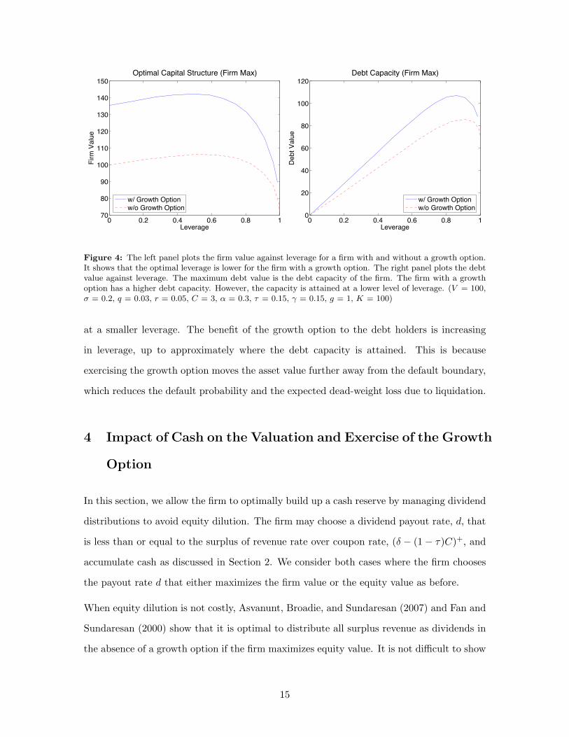
Next we investigate the impact of the growth option on the optimal capital structure of

the firm. The left panel of Figure 4 shows that having a growth option reduces the firm’s

leverage at the optimal capital structure. This is consistent with the empirical observation

that firms with many growth opportunities are not as highly leveraged as the others (Billett

et al. (2007)). We can also see from this plot that the firm benefits more from the growth

option when its leverage is small. This may also be a contributing factor for firms with a

growth option to have lower leverage.

Debt capacity is the maximum value of debt that can be sustained by the firm. The right

panel of Figure 4 shows the growth option’s impact on the debt capacity. We find that the

growth option increases the debt capacity of the firm. However, the capacity is attained

14

0 0.2 0.4 0.6 0.8 170

80

90

100

110

120

130

140

150

Leverage

Firm

Val

ue

Optimal Capital Structure (Firm Max)

w/ Growth Optionw/o Growth Option

0 0.2 0.4 0.6 0.8 10

20

40

60

80

100

120

Leverage

Debt

Val

ue

Debt Capacity (Firm Max)

w/ Growth Optionw/o Growth Option

Figure 4: The left panel plots the firm value against leverage for a firm with and without a growth option.It shows that the optimal leverage is lower for the firm with a growth option. The right panel plots the debtvalue against leverage. The maximum debt value is the debt capacity of the firm. The firm with a growthoption has a higher debt capacity. However, the capacity is attained at a lower level of leverage. (V = 100,σ = 0.2, q = 0.03, r = 0.05, C = 3, α = 0.3, τ = 0.15, γ = 0.15, g = 1, K = 100)

at a smaller leverage. The benefit of the growth option to the debt holders is increasing

in leverage, up to approximately where the debt capacity is attained. This is because

exercising the growth option moves the asset value further away from the default boundary,

which reduces the default probability and the expected dead-weight loss due to liquidation.

4 Impact of Cash on the Valuation and Exercise of the Growth

Option

In this section, we allow the firm to optimally build up a cash reserve by managing dividend

distributions to avoid equity dilution. The firm may choose a dividend payout rate, d, that

is less than or equal to the surplus of revenue rate over coupon rate, (δ − (1− τ)C)+, and

accumulate cash as discussed in Section 2. We consider both cases where the firm chooses

the payout rate d that either maximizes the firm value or the equity value as before.

When equity dilution is not costly, Asvanunt, Broadie, and Sundaresan (2007) and Fan and

Sundaresan (2000) show that it is optimal to distribute all surplus revenue as dividends in

the absence of a growth option if the firm maximizes equity value. It is not difficult to show

15

that this result remains true in the presence of a growth option. Therefore in our model,

the firm is holding cash only when equity dilution is costly, or when it is maximizing the

firm value.

In order to determine the optimal policy for the firm that is maintaining a cash reserve, we

develop a binomial lattice method similar to that of Asvanunt, Broadie, and Sundaresan

(2007). The detailed description and the convergence of the method can be found in Ap-

pendix B. The results presented in the remaining of this paper are obtained by the binomial

procedure with a maturity of 200 years and 9,600 time steps.

4.1 Optimal Exercise Boundary and Cash Level

When the firm is holding cash, the exercise boundary becomes a function of both the asset

value, V , and the cash level, x. Figure 5 shows the optimal exercise boundary for various

equity dilution costs. When there is no cost of equity dilution, the amount of cash the firm

has is irrelevant since it can raise money by diluting equity at no cost. However, with a

positive dilution cost, the optimal exercise boundary is decreasing in x, up to x = K. For

the values of x > K, it is no longer necessary for the firm to dilute equity, and hence the

exercise boundary is the same as in the case of γ = 0. At this point, equity dilution cost

becomes irrelevant. This result is very intuitive. When the firm does not have enough cash

reserve, it has to undergo costly equity dilution to make up for the shortfall. The more

case it needs to raise, the more return it demands from the growth option. Therefore, the

boundary decreases as the level of cash balance increases. For the same reason, the exercise

boundary is increasing in the dilution cost, γ, for any fixed value of cash, x ≤ K. As

observed in Section 3.4, the boundary is lower under the first-best policy than it is under

the second-best policy.

Next, we investigate the optimal level of cash, x∗, which also determines the optimal divi-

dend policy. At any given time, if the current cash level, x, is less than the optimal level,

x∗, then the firm withholds any revenue surplus until x reaches x∗. On the other hand, if

x > x∗, then the firm will pay out x− x∗ as dividends so that it gets to the optimal level.

Figure 6 shows the optimal cash levels with and without the growth option, under the

16

Figure 5: This figure shows the plots of optimal exercise region as a function cash and asset value, underthe first- and second-best policies. The optimal exercise boundary is decreasing with cash level, and becomesconstant after cash exceeds the cost of the exercise. The boundary is increasing in the equity dilution cost, γ,when the amount of cash is less than the cost of the exercise. The boundary is always lower under first-bestpolicy than under second-best policy. (V = 100, σ = 0.2, q = 0.03, r = 0.05, C = 3, α = 0.3, τ = 0.15, γ= 0.15, g = 1, K = 100, rx = 0.05)

0 200 400 600 8000

20

40

60

80

100

120

V

x*

Optimal Level of Cash Balance (Firm Max.)

w/ Growth Optionw/o Growth Option

0 200 400 600 8000

20

40

60

80

100

120

V

x*

Optimal Level of Cash Balance (Equity Max.)

w/ Growth Optionw/o Growth Option

Figure 6: This figure shows the plots of optimal cash level, x∗, versus asset value, V , with and without agrowth option under both first- and second-best policies. Under the first-best policy, x∗ is decreasing withV when the firm has no growth option, and is increasing with V when the firm has a growth option. Underthe second-best policy, the relationship between x∗ and V is similar, except that for the values of V that arevery close to VB , the optimal cash level is zero. This is because equity holders will consume the cash beforedebt holders get it upon liquidation. (V = 100, σ = 0.2, q = 0.03, r = 0.05, C = 3, α = 0.3, τ = 0.15, γ =0.15, g = 1, K = 100, rx = 0.05)

first-best and the second-best policies. First let us consider the first-best policy. Without

a growth option, the firm holds cash to avoid future equity dilution and costly bankruptcy.

The optimal level of cash, x∗, is decreasing with the asset value, V . The higher the value

17

of V , the further away the firm is from equity dilution and bankruptcy, so the incentive for

holding cash is less. Under the second-best policy, x∗ is also decreasing in V , but only when

V is above a certain threshold (V ≥ 25 in Figure 6). The optimal level of cash below this

threshold is zero. This is because when an equity value maximizing firm is very close to

bankruptcy, it will pay out all remaining cash as dividends so that the debt holders will not

get it upon liquidation. The optimal cash level is also generally lower under the second-best

policy for the same reason. With a growth option, the firm will maintain a much higher level

of cash in both cases. The optimal cash level is increasing in V , but never exceeds the cost

of exercising the option, K. This is because at higher values of V , the firm is more likely

to exercise the option so it starts saving toward it. The optimal cash level, x∗, is capped at

K because there is no need to maintain more cash than is necessary to exercise the option.

The same region where the firm does not keep cash still exists under the second-best policy

with a growth option.

Figure 7 shows the impact of agency and equity dilution cost on the optimal cash level when

the firm has a growth option. As expected, agency cost reduces the optimal amount of cash

held inside the firm. As explained earlier, there is no incentive for holding cash under the

second-best policy, as depicted in the right panel of Figure 7. However, under the first-best

policy, it is optimal for the firm to maintain a cash reserve even when equity issuance is

not costly. The left panel of Figure 7 shows that the optimal cash level is decreasing in

V when γ = 0, as opposed to increasing when γ > 0. This is because the sole purpose of

holding cash is to prolong the life of the firm instead of financing the growth option. By

prolonging its life, the firm benefits from receiving more tax deductions and an increase in

the probability of the option getting exercised.

The optimal exercise boundary shown in Figure 5 and the optimal cash level in Figure 6

completely characterize an optimal strategy for the firm. In Figure 8, we superimpose the

two plots onto one another. For simplicity of the discussion, we will refer to xt as the

amount of cash after the coupon payment is made. The optimal strategy is as follows. The

firm makes two decisions sequentially. First, given its current asset value and cash level,

(Vt, xt), it decides whether or not to exercise the option. Suppose that the current state

18

0 100 200 300 400 5000

20

40

60

80

100

120

V

x*

Optimal Level of Cash Balance w/ Growth Option (Firm Max.)

! = 0%! = 15%

0 100 200 300 400 5000

20

40

60

80

100

120

V

x*

Optimal Level of Cash Balance w/ Growth Option (Equity Max.)

! = 0%! = 15%

Figure 7: This figure completely characterizes the optimal policy regarding cash and the exercise of thegrowth option. The left panel corresponds to the decisions before the growth option is exercised. In regionA, the firm will exercise the option, and all subsequent decisions are determined in the right panel. In regionB, V is not high enough to exercise and x is below the optimal level so the firm will not dividends. In regionC, x is above the optimal level so the firm will pay excess above the optimal level as dividend. Once theoption is exercised, the decisions in regions D and E and similar to those in regions B and C, respectively.(V = 100, σ = 0.2, q = 0.03, r = 0.05, C = 3, α = 0.3, τ = 0.15, γ = 0.15, g = 1, K = 100, rx = 0.049)

Figure 8: This figure completely characterizes the optimal policy regarding cash and the exercise of thegrowth option. The left panel corresponds to the decisions before the growth option is exercised. In regionA, the firm will exercise the option, and all subsequent decisions are determined in the right panel. In regionB, V is not high enough to exercise and x is below the optimal level so the firm will not dividends. In regionC, x is above the optimal level so the firm will pay excess above the optimal level as dividend. Once theoption is exercised, the decisions in regions D and E and similar to those in regions B and C, respectively.(V = 100, σ = 0.2, q = 0.03, r = 0.05, C = 3, α = 0.3, τ = 0.15, γ = 0.15, g = 1, K = 100, rx = 0.05)

(Vt, xt) is not in the exercise region A in the left panel. Then it has to decide how much of

its revenue to save and how much to pay out as dividends. If (Vt, xt) is in region B, then

the firm will do nothing (pay no dividend), and will instantaneously move horizontally to

19

(Vt, xt + (qVt − C)dt). Note that depending on the value of Vt, qVt − C could be either

positive or negative. Otherwise, the firm is in region C, and will pay out dividends such

that it instantaneously moves to (Vt, x∗t ). On the other hand, suppose that (Vt, xt) is in

the exercise region A. Then the firm will exercise the option, and instantaneously move to

((1 + g)Vt, (xt −K)+). Then, the decision on the dividend payout depends on whether its

new state is in the region D or E in the right panel. The dividend decision is similar to when

the growth option is not yet exercised. Figure 9 shows how the liquidation cost, α, and the

equity dilution cost, γ, affect boundaries of these regions. We find that when γ increases

from 15% to 30%, region B becomes significantly larger. This is due to a significant increase

in the exercise boundary. The dilution cost has little to no impact on the firm’s decisions

once the option is already exercised. When α decreases from 30% to 0%, we find that region

D becomes significantly smaller as the optimal cash level decreases. However, we find that

the liquidation cost has no significant impact on the firm’s decisions before the option is

exercised. This suggests that the dominating incentive for holding cash for a firm with a

growth option is to finance the option, rather than to avoid bankruptcy.

Figure 9: This figure shows how the equity dilution cost, γ, affects the various regions. Increasing γincreases the region where the firm is neither exercising nor paying out dividend. (V = 100, σ = 0.2, q =0.03, r = 0.05, C = 3, α = 0.3, τ = 0, γ = 0.15, g = 1, K = 100, rx = 0.05)

20

4.2 Values of Holding Cash and a Growth Option

In this section, we investigate the interactions between the growth option and the cash

balance. Specifically, we compare the value of the growth option to the firm when it can

hold cash to when it cannot, and the value of holding cash with and without a growth

option. The left panel of Figure 10 shows the value of the option as a function of γ. As

explained in Section 3.5, the value of the growth option is the difference in the firm (equity)

value between having and not having a growth option. We consider only the results of the

first-best policy in this section. As before, we find the option value is decreasing in γ, but

we find that the decrease is at a much slower rate when the firm is holding a cash reserve.

This is because the firm saves cash to reduce the amount of equity dilution required to

exercise the option. As observed in the previous section, most of the benefit of the option

goes to the shareholders.

0 0.1 0.2 0.3 0.4 0.522

24

26

28

30

32

34

36

!

Opt

ion

Valu

e

Option Value on Firm and Equity (Firm Max.)

Firm w/ Cash BalanceFirm w/o Cash BalanceEquity w/ Cash BalanceEquity w/o Cash Balance

0 0.1 0.2 0.3 0.4 0.5!2

0

2

4

6

8

10

12

!

Cash

Val

ue

Cash Value on Firm and Equity (Firm Max.)

Firm w/ Growth OptionFirm w/o Growth OptionEquity w/ Growth OptionEquity w/o Growth Option

Figure 10: The left panel plots the value of the growth option versus equity dilution cost, γ. The optionvalue is decreasing in γ. It is much less sensitive to γ when the firm is holding cash. The right panel plotsthe value of holding cash against γ. The cash value is increasing in γ. It is much more sensitive to γ whengrowth option is present. In all cases, the growth option and cash balance are more valuable to equityholders than they are to debt holders. (V = 100, σ = 0.2, q = 0.03, r = 0.05, C = 3, α = 0.3, τ = 0.15, g= 1, K = 100, rx = 0.05)

The right panel of Figure 10 shows the value of holding cash, with and without a growth

option, as a function of γ. Similarly, this is the difference between the firm (equity) value of

a firm that optimally accumulates cash reserve and a firm that always pays out dividends in

full. The main purpose of cash is to reduce equity dilution cost, and therefore holding cash is

21

more valuable when the dilution cost is higher. The value of holding cash (in both equity and

firm value) is very small in the absence of a growth option, but increases significantly when

it is present. Under the first-best policy, holding cash may actually have a negative impact

on the equity value when γ is small. However, with a growth option present, its impact

increases rapidly and becomes positive as γ increases. The results in this section illustrate

the importance of cash and the dividend policy for firms with growth opportunities. While

dividend policy may not have significant impact for firms without investment opportunities,

it can be crucial for start-up firms with substantial growth potentials.

4.3 Cash Reserve Properties across Different Firms

A recent empirical study by Acharya et al. (2007) shows that the correlation between the

amount of cash held within a firm and its credit spread is positive. Despite the common

belief that firms with large cash reserves are safer, it may be the case that riskier firms

need cash to remain liquid in order to avoid default and bankruptcy. We use our model to

explore this question. In Figure 11, we reproduce the plot of the optimal cash level (from

Figure 6) in terms of optimal cash-to-asset ratio versus the default probability, which is

a good proxy for credit spread. In this figure, we use the probability that the firm will

default within the next 200 years (the length of our binomial lattice). Our model suggests

that firms with higher spreads should hold more cash than firms with lower spreads. As

explained earlier, this is because risker firms are more likely to have cash flow shortages,

so they hold on to more cash to provide additional liquidity to avoid equity dilution. The

presence of a growth option systematically increases the optimal level of the cash-to-asset

ratio for all firms.

In the previous results, we looked at the optimal cash ratio for firms with different asset

values V , but with the same coupon rate C. What happens if these firms are operating at

their optimal capital structure? Figure 12 compares the optimal cash-to-asset ratio under

the first-best policy between firms with fixed and optimal coupon. We are plotting cash-to-

asset ratio against V instead of the default probability because when C is chosen optimally,

the default probability does not change as the value of V changes. Recall that in absence of

22

0 0.2 0.4 0.6 0.8 10

0.5

1

1.5

2

2.5

3

3.5

Default Probability

Cas

h/As

set R

atio

Optimal Cash!to!Asset Ratio versus Default Probability (Firm Max)

w/ Growth Optionw/o Growth Option

0 0.2 0.4 0.6 0.8 10

0.5

1

1.5

2

2.5

3

Default Probability

Cash

/Ass

et R

atio

Optimal Cash!to!Asset Ration versus Default Probability (Equity Max)

w/ Growth Optionw/o Growth Option

Figure 11: This figure plots the optimal cash-to-asset ratio, under first- and second-best policies, againstthe default probability. Under the first-best policy, optimal cash-to-asset ratio is increasing with defaultprobability. Under the second-best policy, it is also increasing, but only up to a value of probability close toone. Beyond that, the optimal cash ratio is zero. (V = 100, σ = 0.2, q = 0.03, r = 0.05, C = 3, α = 0.3, τ= 0.15, γ = 0.15, g = 1, K = 100, rx = 0.05)

a growth option, cash is solely used for protection against costly dilution in the bad states.

Hence we find that the optimal cash-to-asset ratio is constant with respect to V under the

optimal leverage, because C proportionately increases or decreases with V . When a growth

option is present, however, firms with lower asset values hold more cash than firms whose

asset values are higher. This is because the optimal leverage takes into account the future

exercise of the growth option. As such, the coupon level is considerably high for the current

asset level, and firms with low asset values will hold a large amount of cash to ensure that

they survive long enough to exercise the option. Intuitively, the amount of cash these firms

hold decreases as V increases. In the fixed coupon case, we choose C to be the optimal

coupon for V = 100. Consequently, we find that the optimal cash ratio is higher for the

fixed coupon case than it is for the optimal coupon case when V < 100, and lower when

V > 100.

5 Extension: Multiple Growth Options

The binomial method described in Appendix B can be easily extended to evaluate firms

with multiple growth options of different sizes and cost structures. Appendix C provides a

23

0 50 100 150 200 250 3000

1

2

3

4

5

6Optimal Cash!to!Asset Ratio versus Asset Value

Asset Value

Cash

/Ass

et R

atio

w/ Growth Option ! Fixed Couponw/o Growth Option ! Fixed Couponw/ Growth Option ! Optimal Couponw/o Growth Option ! Optimal Coupon

Figure 12: The figure plots the optimal cash-to-asset ratio versus the asset value, V , for a firm with andwithout a growth option, for both fixed and optimal leverage case. Without a growth option, the optimalcash ratio is decreasing in V when C is fixed. It is constant in V when C is chosen optimally. With a growthoption, the optimal cash ratio is decreasing in V for both fixed and optimal C. (V = 100, σ = 0.2, q = 0.03,r = 0.05, C = 3 (for fixed coupon), α = 0.3, τ = 0.15, γ = 0.15, g = 1, K = 100, rx = 0.05)

detailed description of the binomial method for multiple options, when their sizes and costs

are the same. For a simple illustration, we consider the first-best policy of a firm with a

single opportunity to acquire two additional units of its current asset (g1 = 2) at a cost of

K1 = 2V0, and a firm with two opportunities to acquire a single unit (g2 = 1) at a cost

K2 = V0 each time. Essentially, we are comparing between at a firm that must expand its

operation in one execution to a firm that can expand its operation by the same amount, but

in multiple phases (two in this example). We can also think of these as the same option,

where one must be exercised once, while the other can be exercised in two halves. The

left panel of Figure 13 shows the optimal exercise boundaries for the two cases. Compared

with the boundary of the option with a single exercise, we find that the boundary for the

first (of two) exercise is lower, while that for the second (of two) exercise is higher. The

right panel of Figure 13 shows the optimal cash level before and after each of the exercises.

The optimal cash level is increasing up to $200, when there are two exercises left, and only

up to $100, when there is only one exercise left. Once all the options are exercised, the

optimal cash level for both cases are the same. Figure 14 plots the option value against

equity dilution cost, γ. It shows that the option value increases when it can be exercised it

in two halves, and that the difference is increasing in γ. The option becomes more valuable

24

because the firm does not need to accumulate as much cash for each exercise.

Figure 13: The left panel compares the exercise boundaries for a firm with one and two options. Boundaryfor the first (of two) exercise is lower than that of a single option, while the boundary for the second (of two)exercise is higher. The right panel shows the optimal cash levels. For the cash of two options, the optimalcash level is increasing up to $200 before the 1st option is exercised, and up to $100 after the it is exercised.Once all options are exercised, the optimal cash level is the same as the single option case. (V = 100, σ =0.2, q = 0.03, r = 0.05, C = 3 (for fixed leverage), α = 0.3, τ = 0.15, γ = 0.15, g1 = 2, g2 = 1, K1 = 200,K2 = 100, rx = 0.05)

0 0.1 0.2 0.3 0.4 0.556

58

60

62

64

66

68

70

72

!

Opt

ion

Valu

e

Option Value on Firm and Equity: 1 vs 2 Exercises

Firm w/ Single ExerciseFirm w/ 2 ExercisesEquity w/ Single ExerciseEquity w/ 2 Exercises

Figure 14: The figure compares the value of growth option between 1 and 2 exercises. The ability toexercise in 2 steps increases the value of the option. The increase is larger when equity dilution is morecostly. (V = 100, σ = 0.2, q = 0.03, r = 0.05, C = 3 (for fixed leverage), α = 0.3, τ = 0.15, γ = 0.15, g1 =2, g2 = 1, K1 = 200, K2 = 100, rx = 0.05)

25

6 Conclusions

In this paper, we investigate optimal decisions for companies with growth opportunities.

First, we provide analytical solutions for the firm’s security values when equity dilution is

costly and dividends are paid out in full (i.e., no cash reserve). We show that firms with

growth opportunities have lower leverage at the optimal capital structure. We model capital

market friction by assuming that equity dilution is costly. A binomial method is developed

to determine the optimal dividend policy and the optimal exercise boundary of the growth

option. We completely characterize the firm’s optimal strategy by computing the regions

where the firm exercises the option, builds up a cash reserve, and distributes dividends. The

choice of dividend policy is shown to be extremely important when the firm has investment

opportunities, as illustrated by a significant increase in the firm value when it is permitted

to hold cash. We also investigate why different firms across different rating categories carry

different amounts of cash. We show that the optimal cash-to-asset ratio is increasing with

the default probability.

Finally, we illustrate how our binomial method can be extended to evaluate firms with

multiple growth opportunities. Through a simple example, we show how the firm’s policy

changes if it can implement the expansion in two phases rather than one.

26

Appendix A

Derivation for Equity Value in Section 3.1

Writing the general solution (3) for E(V ) as

E(V ) =

A0 +A1V +A2V−Y +A3V

−X for VB ≤ V ≤ C/q

A0 + A1V + A2V−Y + A3V

−X for C/q ≤ V ≤ VG,(16)

and substitute it in (6), we get

12σ

2A2Y (Y + 1)V −Y + 12σ

2A3X(X + 1)V −X − (r − q)A1V − (r − q)A2Y V−Y

−(r − q)A3XV−X − r(A0 +A1V +A2V

−Y +A3V−X) + β(qV − C) = 0

(17)

A0 and A1 can be solved by collecting the constant and the coefficient of the linear term in

(17) as follows:

−rA0 − βC = 0⇒ A0 = −βCr

(r − q)A1 − rA1 + βq = 0⇒ A1 = β

Similarly, we can substitute (16) in (7) and solve for the coefficients A0 and A1.

−rA0 − C = 0⇒ A0 = −Cr

(r − q)A1 − rA1 + β = 0⇒ A1 = 1

A2, A3, A2 and A3 are determined by solving the system of four linear equations imposed

27

by the conditions in (8), namely

A2V−YB +A3V

−XB + βVB −

βC

r= 0 (18)

A2

(C

q

)−Y

+A3

(C

q

)−X

+βC

q− βC

r= A2

(C

q

)−Y

+ A3

(C

q

)−X

+C

q− C

r(19)

−A2Y

(C

q

)−Y−1

−A3X

(C

q

)−X−1

+ β = −A2Y

(C

q

)−Y−1

− A3X

(C

q

)−X−1

+ 1 (20)

A2V−YG + A3V

−XG + VG −

C

r= (1 +G)VG −

C

r− βK (21)

+[(β − 1)

(C

q− C

r

)(V 0

B

)−X+ β

(C

q

)−X (C

r−(V 0

B

))] (V 0

B

)X+Y((1 + g)VG)−X

+ (β − 1)(XC

r−XC

q− C

q

)((V 0

B

)−X −(V 0

B

)−Y(C

q

)Y−X) (

V 0B

)X+Y

X − Y((1 + g)VG)−X ,

where V 0B is the bankruptcy boundary of a firm without a growth option.

Hence the equity value before exercising the growth option is given by

E(V ) =

−βCr + βV +A2V

−Y +A3V−X for V 0

B ≤ V < C/q

−Cr + V + A2V

−Y + A3V−X for C/q ≤ V ≤ VG,

where

A2 =1

qr(Y −X) (V YB V X

G − V XB V Y

G )

(V Y

B ((g + 1)VG)−X (V 0B

)−Y

(C

(C

q

)Y

(Xr + r − qX)(β − 1)

V XG

(V 0

B

)Y((g + 1)VG)X +

(q(X − Y )βV X

B (C − rVB) − C

(C

q

)X

(Y r + r − qY )(β − 1)

)

V YG

(V 0

B

)Y((g + 1)VG)X − gqr(X − Y )V X+Y +1

G

(V 0

B

)Y((g + 1)VG)X + V X+Y

G

(− C

(C

q

)Y

(Xr + r − qX)(β − 1)(V 0

B

)X+

(C(Y r + r − qY )(β − 1)

(C

q

)X

+Kqr(X − Y )β ((g + 1)VG)X

)(V 0

B

)Y − Cq(X − Y )β(V 0

B

)X+Y+ qr(X − Y )β

(V 0

B

)X+Y +1

)))

28

A3 =1

qr(Y −X) (V YB V X

G − V XB V Y

G )

(V X

B ((g + 1)VG)−X (V 0B

)−Y

((q(Y −X)βV Y

B (C − rVB) − C

(C

q

)Y

(Xr + r − qX)(β − 1)

)V X

G

(V 0

B

)Y((g + 1)VG)X + C

(C

q

)X

(Y r + r − qY )(β − 1)V YG

(V 0

B

)Y((g + 1)VG)X + gqr(X − Y )V X+Y +1

G

(V 0

B

)Y((g + 1)VG)X + V X+Y

G

(C

(C

q

)Y

(Xr + r − qX)(β − 1)

(V 0

B

)X+

(−C(Y r + r − qY )(β − 1)

(C

q

)X

−Kqr(X − Y )β ((g + 1)VG)X

)(V 0

B

)Y+ Cq(X − Y )

β(V 0

B

)X+Y − qr(X − Y )β(V 0

B

)X+Y +1

)))

A2 =1

qr(Y −X) (V YB V X

G − V XB V Y

G )

(V Y

G ((g + 1)VG)−X (V 0B

)−Y

(gqr(Y −X)V Y

B V X+1G

(V 0

B

)Y((g + 1)VG)X

+ qr(X − Y )βV YB

(V 0

B

)Y ((V 0

B

)X+1V X

G + ((g + 1)VG)X(KV X

G − V X+1B

))− C

(V Y

B V XG(

− (Y r + r − qY )(β − 1)(V 0

B

)Y (Cq

)X

+ (Xr + r − qX)(β − 1)(V 0

B

)X (Cq

)Y

+ q(X − Y )β(V 0

B

)X+Y

)

−

(−(Y r + r − qY )(β − 1)V Y

B

(C

q

)X

+ (Xr + r − qX)(β − 1)V XB

(C

q

)Y

+ q(X − Y )βV X+YB

)

((g + 1)VG)X (V 0B

)Y )))

A3 =1

qr(Y −X) (V YB V X

G − V XB V Y

G )

(V X

G ((g + 1)VG)−X (V 0B

)−Y

(gqr(X − Y )V Y +1

G ((g + 1)VG)X (V 0B

)YV X

B + qr(Y −X)β(V 0

B

)Y ((KV Y

G − V Y +1B

)((g + 1)VG)X + V Y

G

(V 0

B

)X+1)V X

B − C

(V Y

G

((Y r + r − qY )

(β − 1)(V 0

B

)Y (Cq

)X

− (Xr + r − qX)(β − 1)(V 0

B

)X (Cq

)Y

− q(X − Y )β(V 0

B

)X+Y

)V X

B +(−(Y r + r − qY )(β − 1)V Y

B

(C

q

)X

+ (Xr + r − qX)(β − 1)V XB

(C

q

)Y

+ q(X − Y )βV X+YB

)

((g + 1)VG)X (V 0B

)Y )))

29

Derivation for Debt Value in Section 3.2

Substituting the general solution (10) into (9), we get:

12σ2B2X(X + 1)V −X + (r − q)B1V − (r − q)B2XV

−X

− r(B0 +B1V +B2V−X) + C = 0 (22)

B0 and B1 can be solved by collecting the constant and the coefficient of the linear term in

(22) as follows:

−rB0 + C = 0⇒ B0 =C

r

(r − q)B1 − rB1 = 0⇒ B1 = 0

B2 and B3 are determined by solving the system of linear equations imposed by the bound-

ary conditions in (11), namely

C

r+B2V

−YB +B3V

−XB = (1− α)VB (23)

C

r+B2V

−YG +B3V

−XG =

C

r+(

(1− α)V 0B −

C

r

)((1 + g)VV 0B

)−X, (24)

Thus the debt value is given by

D(V ) =C

r+B2V

−Y +B3V−X , (25)

30

where

B2 =(VBVG)Y ((1 + g)VG)−X(

V YB V

XG − V X

B V YG

) [((1 + g)VG)XV X

B(C

r− (1− α)VB

)− V X

G

(V 0B

)X (Cr− (1− α)V 0

B

)](26)

B3 = −(VBVG)X ((1 + g)VG)−X(V YB V

XG − V X

B V YG

) [((1 + g)VG)XV Y

B(C

r− (1− α)VB

)− V Y

G

(V 0B

)X (Cr− (1− α)

(V 0B

))](27)

Appendix B

Binomial Lattice Method for Growth Option with Cash Balance

We extend the binomial lattice method of Broadie and Kaya (2007) and Asvanunt, Broadie,

and Sundaresan (2007) to evaluate the securities values in the presence of growth option

and cash balances. Following Cox et al. (1979), we divide time into N increments of length

h = T/N , then we write the evolution of the firm asset value Vt as follows:

Vt+h =

uVt with risk-neutral probability p

dVt with risk-neutral probability 1− p

Let V ut = uVt and V d

t = dVt. By imposing that u = 1/d, we have:

u = eσ√h

d = e−σ√h

a = e(r−q)h

p =a− du− d

In this setting, we approximate revenue during time interval h by:

∫ t+h

tqVtdt ≈ Vt(eqh − 1) =: δt

31

Similarly, we approximate the coupon payment by:

∫ t+h

tcPdt ≈ P (ech − 1) =: ζ

Incorporating the tax benefit of rate τ , the effective coupon payment is (1− τ)ζ.

We need to construct two lattices, one for the values before the growth option is exercised,

and another for the values after the growth option is exercised. Recall that when the firm

decides to exercise the growth option, the asset value increases from V to (1 + g)V . We

will denote the asset values in the exercised lattice by V = (1 + g)V , and all other security

values by E and D, etc.

Each node in the lattice is a vector of dimension M , where each element in the vector

corresponds to a different level of cash balance, x. The values of x are linearly spaced from

0 to xmax.4

We distinguish the cash before and cash after revenue and dividend by x and x+, respec-

tively.

Let Et(Vt, xt) be the equity value at time t when the firm’s asset value is Vt, and its

cash balance level is xt. Similarly, Dt(Vt, xt) is the corresponding debt value. We also let

Et[ft+h(Vt+h, xt+h)] be the expected value of the security f(·) at the next time period t+h,

given the information at time t, where f(·) can represent the equity value, E(·), or the debt

value, D(·), namely,

Et[ft+h(Vt+h, xt+h)] = pft+h(V ut+h, xt+h) + (1− p)ft+h(V d

t+h, xt+h).

Note that xt+h is deterministic because it only depends on the decision at time t. Since we

only know the values of ft+h(V, x) for a discrete set of values of x, we use linear interpolation

to estimate ft+h(V ut+h, xt+h) and ft+h(V d

t+h, xt+h).

Figure 15 illustrates what each node in the two lattices represents.4In our routine, we pick xmax arbitrarily and check if the optimal cash balance, x∗, is attained at xmax.

If it does, then we increase xmax and repeat the routine.

32

! "0,tt Vf . . .

! "max, xVf tt

! "0,uhtht Vf ##

.

.

. ! "max, xVf u

htht ##

! "0,dhtht Vf ##

.

.

. ! "max, xVf d

htht ##

p

1 – p

! "0,~~tt Vf

.

.

. ! "max,~~ xVf tt

! "0,~~ uhtht Vf ##

.

.

. ! "max,~~ xVf u

htht ##

! "0,~~ dhtht Vf ##

.

.

. ! "max,~~ xVf d

htht ##

p

1 – p

After Exercise

Before Exercise

Figure 15: This figure illustrates the vector in each node of the lattices. ft(·) in the lower lattice representsthe security value at each element of the vector before the growth option is exercised. ft(·) in the upperlattice represents the security value after the growth option is exercised.

First, we construct the exercised lattice. At maturity, the firm returns everything to share-

holders after meeting its debt obligations.

If VT + xT + δT ≥ (1− τ)ζ + P :

ET (VT , xT ) = VT + xT + δT − (1− τ)ζ − P

DT (VT , xT ) = ζ + P

If (VT , xT ) is such that the firm does not have enough value to meet its debt obligation, it

declares bankruptcy and liquidates its assets.

If VT + xT + δT < (1− τ)ζ + P :

ET (VT , xT ) = 0

DT (VT , xT ) = (1− α)(VT + xT + δT )

33

At other times t, if (Vt, xt) is such that the firm has enough cash from revenue and cash

balance to meet its debt obligations, then it has an option to retain some excess revenue in

the cash balance, or pay it out to shareholders as dividend.

1. If xt + δt ≥ (1− τ)ζ:

Choose x+t ∈ [0, xt + δt − (1− τ)ζ]

xt+h = erxhx+t

Et(Vt, xt) = e−rhEt[Et+h(Vt+h, xt+h)

]+ xt + δt − (1− τ)ζ − x+

t

Dt(Vt, xt) = e−rhEt[Dt+h(Vt+h, xt+h)

]+ ζ

x+t is chosen such that the objective value (firm or equity value) is maximized at time t.

The optimization is done by performing a search over K discrete points of feasible values

of x+t as given above.

If (Vt, xt) is such that the firm does not have enough from revenue and cash balance, then

it has to raise money by diluting equity.

2. If xt + δt < (1− τ)ζ:

If (Vt, xt) is such that the firm has enough equity to cover the shortfall:

2A. If (1− γ)e−rhEt[Et+h(Vt+h, 0)] ≥ (1− τ)ζ − xt − δt:

Et(Vt, xt) = e−rhEt[Et+h(Vt+h, 0)

]+ (xt + δt − (1− τ)ζ)/(1− γ)

Dt(Vt, xt) = e−rhEt[Dt+h(Vt+h, 0)

]+ ζ

If (Vt, xt) is such that the firm does not have enough equity value to cover the shortfall,

then it declares bankruptcy:

2B. If (1− τ)ζ − xt − δt > (1− γ)e−rhEt[Et+h(Vt+h, 0)]

Et(Vt, xt) = 0

Dt(Vt, xt) = (1− α)(Vt + xt + δt)

34

Once we know the securities values if the option is immediately exercised, we compute its

current value by comparing the continuation value with the exercised value. For each node

(Vt, xt), the continuation values is determined by the exact same routine as the exercised

values, with Vt and δt replaced by Vt and δt.

Let EXt and DXt be the equity and debt values if the firm exercises the growth option at

time t. These values can be determined as follow.

If (Vt, xt) is such that the firm has enough cash after making the coupon payments to

exercise the option.

1. If xt + δt − (1− τ)ζ > K:

EXt (Vt, xt) = Et(Vt, xt + δt − (1− τ)ζ −K)

DXt (Vt, xt) = Dt(Vt, xt + δt − (1− τ)ζ −K)

If (Vt, xt) is such that the firm does not have enough cash to exercise the option, then it

has to raise money by diluting equity.

2. If xt + δt − (1− τ)ζ < K:

EXt (Vt, xt) = Et(Vt, 0) + (xt + δt − (1− τ)ζ −K)/(1− γ)

DXt (Vt, xt) = Dt(Vt, 0)

Then at each node, we simply replace the values of Et and Dt by EXt and DXt if EXt +

DXt > Et + Dt under the firm value maximization, or if EXt > Et under the equity value

maximization. Note that if the firm does not have enough equity to dilute to exercise the

option, then EXt will be negative and the option will not be exercised.

To determine the rate of convergence of this method, we set rx = −∞ to force the firm to

pay out maximum dividend (not holding any cash). In this case, the results converge to the

security values derived in Section 3.

Figure 16 below shows the convergence results of the binomial routine under costly equity

dilution, for both equity and firm value maximization. As in Broadie and Kaya (2007), the

equity value converges linearly to the true value while the error on the debt value oscillates

35

sharply.

102 103 104 10510!3

10!2

10!1

100

101

N

Abso

lute

Erro

rConvergence of Binomial Method (Firm Max.)

EquityDebt

102 103 104 10510!3

10!2

10!1

100

101

N

Abso

lute

Erro

r

Convergence of Binomial Method (Equity Max.)

EquityDebt

Figure 16: Convergence of Binomial Method for Equity and Debt Values.

Appendix C

Extension of Binomial Method for Multiple Growth Options

The binomial method described in Appendix B can be easily modified to handle multiple

options. Let H be the number of options the firm has. Then for each state (Vt, xt) in the

lattice, we add yet another dimension of length H + 1. Therefore, each state of the lattice

becomes (Vt, xt, ht), where ht is the number of options left for exercise. In order to keep

the size of each option consistent with each other, we assume that asset value increases by

gVt(0), where Vt(0) is the current asset value if the firm has never exercised the option. This

is equivalent to having options to acquire g unit of the original asset each time it exercises.

The first step is to compute the continuation values of Et and Dt at each state (Vt, xt, ht),

exactly as described in Appendix B. Then we need to determine whether or not to exercise

the option as follow.

For the states with ht > 0, if (Vt, xt, ht) is such that the firm has enough cash after making

the coupon payments to exercise the option.

36

1. If xt + δt − (1− τ)ζ > K:

EXt (Vt, xt, ht) = Et(Vt + gVt(0), xt + δt − (1− τ)ζ −K,ht − 1)

DXt (Vt, xt, ht) = Dt(Vt + gVt(0), xt + δt − (1− τ)ζ −K,ht − 1)

If (Vt, xt, ht) is such that the firm does not have enough cash to exercise the option, then it

has to raise money by diluting equity.

EXt (Vt, xt, ht) = Et(Vt + gVt(0), 0, ht − 1) + (xt + δt − (1− τ)ζ −K)/(1− γ)

DXt (Vt, xt, ht) = Dt(Vt + gVt(0), 0, ht − 1)

Then, we decide whether or not to exercise the option by comparing either EXt + DXt to

Et +Dt for firm value maximization, or EXt to Et for equity value maximization.

37

References

Acharya, V. V., S. A. Davydenko, and I. A. Strebulaev (2007). Cash Holdings and CreditSpreads. Working Paper, London Business School.

Asvanunt, A., M. Broadie, and S. M. Sundaresan (2007). Managing Corporate Liquidity:Welfare and Pricing Implications. Working Paper, Columbia University.

Billett, M. T., T.-H. D. King, and D. C. Mauer (2007). Growth Opportunities and theChoice of Leverage, Debt Maturity, and Covenants. Journal of Finance 62 (2), 697–730.

Black, F. and J. C. Cox (1976). Valuing Corporate Securities: Some Effects of BondIndenture Provisions. Journal of Finance 31 (2), 351–367.

Boyle, G. W. and G. A. Guthrie (2003). Investment, Uncertainty, and Liquidity. Journalof Finance 58 (5), 2143–2166.

Brennan, M. J. and E. S. Schwartz (1985). Evaluating Natural Resource Investments.Journal of Business 58 (2), 135–57.

Broadie, M. and O. Kaya (2007). A Binomial Lattice Method for Pricing. Corporate Debtand Modeling Chapter 11 Proceedings. Journal of Financial and Quantitative Analy-sis 42 (2), 279–312.

Choe, H., R. Masulis, and V. Nanda (1993). Common Stock Offerings Across the BusinessCycles: Theory and Evidence. Journal of Empirical Finance 1 (1), 3–31.

Corwin, S. A. (2003). The Determinants of Underpricing for Seasoned Equity Offers. Journalof Finance 58 (5), 2249–2279.

Cox, J. C., S. Ross, and M. Rubinstein (1979). Option Pricing: A Simplified Approach.Journal of Financial Economics 7, 633–664.

Decamps, J.-P. and S. Villeneuve (2007). Optimal Dividend Policy and Growth Option.Finance and Stochastic 11 (1), 3–27.

Dixit, A. K. and R. S. Pindyck (1994). Investment under Uncertainty. Princeton UniversityPress, Princeton, NJ.

Duffie, D. (1988). An Extension of the Black-Scholes Model of Security Valuation. Journalof Economic Theory 46 (1), 194–204.

Fan, H. and S. M. Sundaresan (2000). Debt Valuation, Renegotiations, and Optimal Divi-dend Policy. The Review of Financial Studies 13 (4), 1057–1099.

Hirth, S. and M. Uhrig-Homburg (2006). Investment Timing and Endogenous Default.Working Paper, University of Karlsruhe.

Jeanblanc-Picque, M. and A. N. Shiryaev (1995). Optimization of the Flow of Dividends.Russian Mathematical Surveys 50, 257–277.

Leland, H. E. (1994). Corporate Debt Value, Bond Covenants, and Optimal Capital Struc-ture. Journal of Finance 49 (4), 1213–1252.

38

Leland, H. E. and K. B. Toft (1996). Optimal Capital Structure, Endogenous Bankruptcy,and the Term Structure of Credit Spreads. Journal of Finance 51 (3), 987–1019.

Longstaff, F. A. and E. S. Schwartz (1995). A Simple Approach to Valuing Risky Fixedand Floating Rate Debt. Journal of Finance 50 (3), 789–819.

Mauer, D. C. and S. H. Ott (2000). Agency Costs, Underinvestment, and Optimal CapitalStructure: The Effect of Growth Options to Expand. In M. J. Brennan and L. Trigeorgis(Eds.), Project Flexibility, Agency, and Competition, pp. 151–180. Oxford UniversityPress, NY.

Mauer, D. C. and S. Sarkar (2005). Real Options, Agency Conflicts, and Optimal CapitalStructure. Journal of Banking & Finance 29 (6), 1405–1428.

McDonald, R. L. and D. Siegel (1986). The Value of Waiting to Invest. Quarterly Journalof Economics 101 (4), 707–727.

Merton, R. C. (1974). On the Pricing of Corporate Debt: The Risk Structure of InterestRates. Journal of Finance 29 (2), 449–470.

Moyen, N. (2007). How Big is the Debt Overhang Problem? Journal of Economic Dynamicsand Control 31 (2), 433–472.

Radner, R. and L. Shepp (1996). Risk vs. Profit Potential: A Model for Corporate Strategy.Journal of Economic Dynamics and Control 20 (8), 1373–1393.

Sundaresan, S. M. and N. Wang (2007a). Dynamic Investment, Capital Structure, and DebtOverhang. Working Paper, Columbia University.

Sundaresan, S. M. and N. Wang (2007b). Investment under Uncertainty with StrategicDebt Service. Forthcoming, American Economic Review Papers & Proceedings.

Titman, S. and S. Tsyplakov (2006). A Dynamic Model of Optimal Capital Structure.McCombs Research Paper Series No. FIN-03-06, University of Texas at Austin.

39