Neighborhood Risk Factors and Elementary School Achievement in the San Francisco Bay AreaNicole Tirado-Strayer, Koshlan Mayer-Blackwell, Becca Siegel, & Nicholas Biddle

Cartographic Model – November 22, 2013

1. Introduction and OverviewProblem StatementPrevious research shows that poverty and other neighborhood risk factors negatively impact childhood academic achievement.1 Causal mechanisms, however, are unclear. The majority of research modeling the effect of neighborhoods on school performance has been limited to examining correlations census tract data and school level outcomes.2 Researchers have identified several methodological shortcomings to this approach – shortcoming which we can overcome using spatial analysis tool.3 For instance, it is difficult to determine complete demographic data for schools without accurate addresses for each study, and that data alone may fail to differentiate between the consequences of poverty in the home versus negative neighborhood effects on a child’s school.

Research GoalsIn this project, we will build on past research designs to develop a new spatial analysis strategy based on assessing school neighborhoods. Geospatial tools allow for an analysis that would otherwise be impossible: instead of focusing on where students live, we wish to assess how the location of a school itself affects the academic achievement of the students who attend that school. We hypothesize that schools that are located closer to areas characterized as “high risk” will have lower academic achievement than schools that are located further from these areas.

1) Where in the San Francisco Bay Area are neighborhood risk factors spatially concentrated? These risk factors include low median income, low education, high unemployment, racial demographics, high distance from parks or green spaces and high noise pollution.

2) What is the distance from each elementary school to these risk factors?

3) Does the addition of school neighborhood predictors (noise, green space, etc.) improve the accuracy of school achievement predictions based only on demographic data?

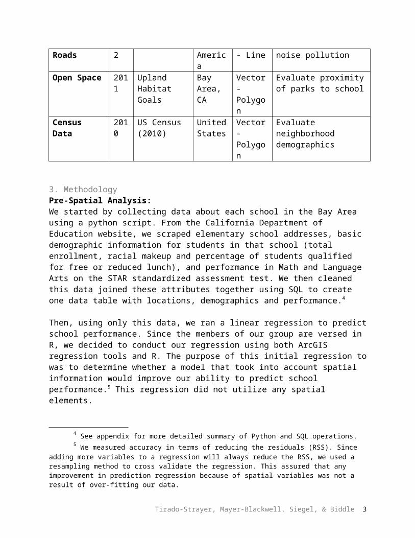
2. Data Sources

1 Brooks-Gunn, J., & Duncan, G. J. (1997). The Effects of Poverty on Children. The Future of Children, 7(2), 55-71.

2 Saporito, S., & Sohoni, D. (2007). Mapping Educational Inequality: Concentrations of Poverty among Poor and Minority Students in Public Schools. Social Forces, 85(3), 1227-1253.

3 Sampson, R., Morenoff, J. D., Gannon-Rowley, T. (2002). Assessing ‘Neighborhood Effects’: Social Processes and New Directions in Research.

Tirado-Strayer, Mayer-Blackwell, Siegel, & Biddle 1

Initial data sources:Year Source Extent Type Purpose

Counties 2012

Esri United States

Vector - Polygon

Determine scope of Bay Area as defined by 9 counties

School Addresses

2012

CA Department of Education

Bay Area, CA

Data Table

Locate elementary schools in the Bay Area

School Demographics

2012

CA Department of Education

Bay Area, CA

Data Table

Account for racial and free/reduced lunch demographics within each school

School Performance

2011

CA Department of Education

Bay Area, CA

Data Table

Measure effect of variables on STAR scores at each school

Major Roads 2012

Esri North America

Vector - Line

Use as proxy for noise pollution

Open Space 2011

Upland Habitat Goals

Bay Area, CA

Vector - Polygon

Evaluate proximity of parks to school

Census Data 2010

US Census (2010)

United States

Vector - Polygon

Evaluate neighborhood demographics

3. MethodologyPre-Spatial Analysis:We started by collecting data about each school in the Bay Area using a python script. From the California Department of Education website, we scraped elementary school addresses, basic demographic information for students in that school (total enrollment, racial makeup and percentage of students qualified for free or reduced lunch), and performance in Math and Language Arts on the STAR standardized assessment test. We then cleaned this data joined these attributes together using SQL to create one data table with locations, demographics and performance.4

Then, using only this data, we ran a linear regression to predict school performance. Since the members of our group are versed in R, we decided to conduct our regression using both ArcGIS regression tools and R. The purpose of this initial regression to was to determine whether a model that took into account spatial information would improve our ability to predict school performance.5 This regression did not utilize any spatial elements.

4 See appendix for more detailed summary of Python and SQL operations. 5 We measured accuracy in terms of reducing the residuals (RSS). Since adding more variables to a

regression will always reduce the RSS, we used a resampling method to cross validate the regression. This assured that any improvement in prediction regression because of spatial variables was not a result of over-fitting our data.

Tirado-Strayer, Mayer-Blackwell, Siegel, & Biddle 2

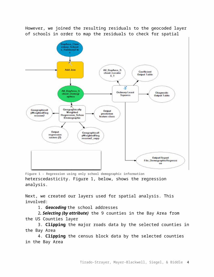
However, we joined the resulting residuals to the geocoded layer of schools in order to map the residuals to check for spatial heterscedasticity. Figure 1, below, shows the regression analysis.

Next, we created our layers used for spatial analysis. This involved:1. Geocoding the school addresses 2. Selecting (by attribute) the 9 counties in the Bay Area from the US Counties layer3. Clipping the major roads data by the selected counties in the Bay Area4. Clipping the census block data by the selected counties in the Bay Area5. Deleting fields containing irrelevant census data (in order to reduce size)6. Normalizing for differing populations of census block groups by creating new fields that calculated percent of adults without any college, percent African American, and percent Latino.

Figure 2, below, shows the model used for the pre-spatial analysis outlined above.

Tirado-Strayer, Mayer-Blackwell, Siegel, & Biddle

Figure 1 - Regression using only school demographic information

3

Finally, we reprojected each of the created layers into California State Plane III (Feet). Our entire study area is contained in California State Plane III.

Figure 2 - Pre-spatial analysis model

Tirado-Strayer, Mayer-Blackwell, Siegel, & Biddle 4

Spatial AnalysisAfter the above steps, we were left with the following layers for analysis:1. Bay Area Elementary Schools (with data) (Vector – Point)2. Bay Area Major Roads (Vector – Line)3. Bay Area Open Space (Vector – Polygon)4. Bay Area Census Block Groups (with selected, normalized data) (Vector – Polygon)

Roads:Distance to nearest major roads was a proxy variable for noise pollution. Since the effects of being close to a major road are only substantial within 100 feet of the road, we created a 100-foot buffer around the major roads. Then, we did a spatial join between the Bay Area School layer and the Roads Buffer, keeping only schools that fell completely within the Roads Buffer. We then created a binary variable for proximity to roads – schools received a “1” if they fell within the Roads Buffer, and a “0” if they did not. This became part of our final regression.

Open Space:We used the near tool to determine the distance between each school and its closest open space.

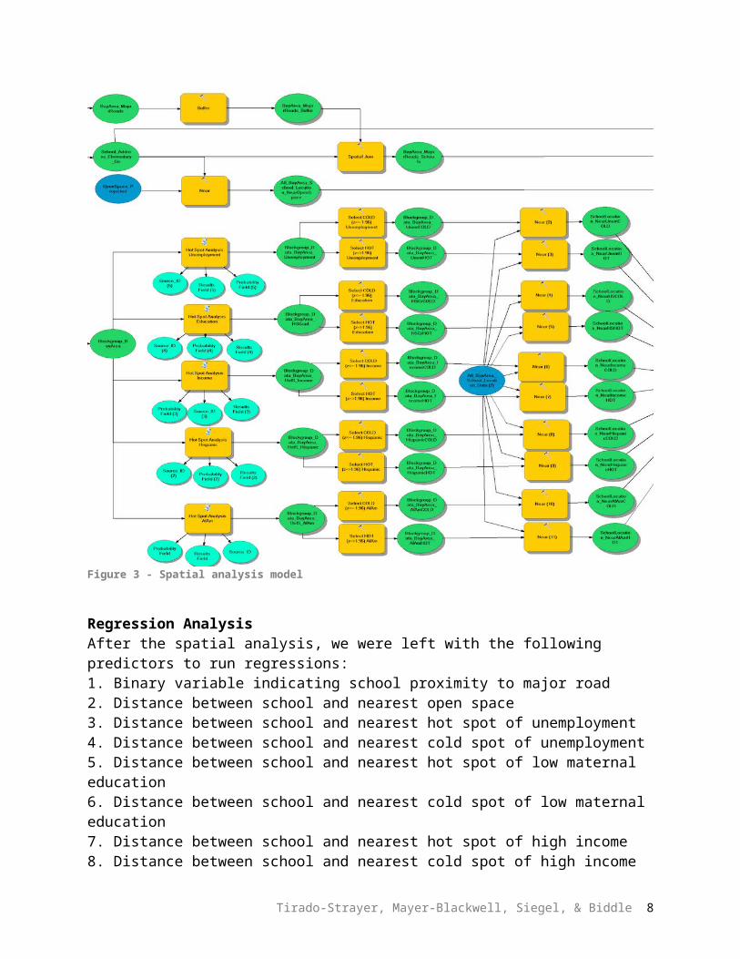
Census Block Group Data: We performed a hot spot analysis on each variable: unemployment, education, income, percent African American, and percent Hispanic. Next, using the output layer from the hot spot analysis, we selected by attribute to determine block groups where the z-score was greater than or equal 1.96 – these were our hot spots for each variable. We also selected by attribute to determine block groups where the z-scores were less than or equal to -1.96 – these were our cold spots for each variable. Finally, we used the near tool to determine the distance between each school and the nearest hot and cold spot for each census variable.

Figure 3, below, shows the model for our spatial analysis processes.

Tirado-Strayer, Mayer-Blackwell, Siegel, & Biddle 5

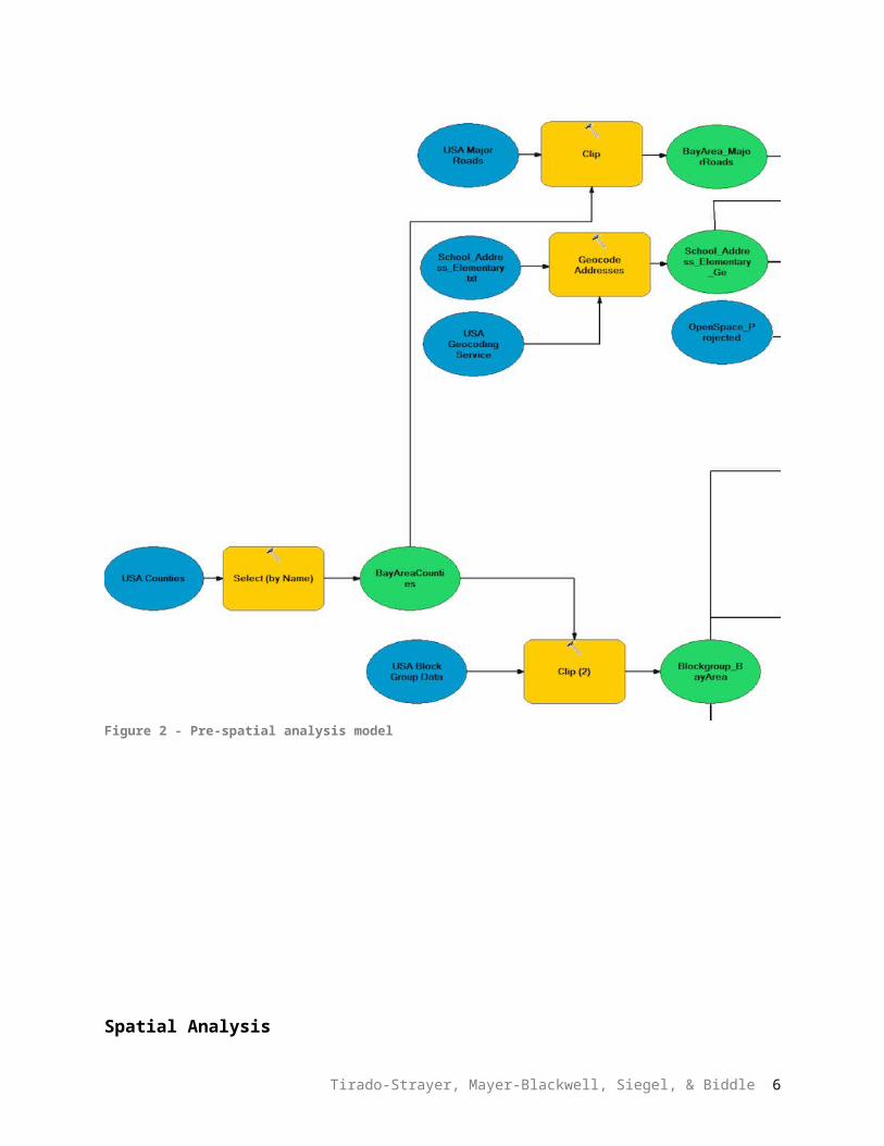
Figure 3 - Spatial analysis model

Regression AnalysisAfter the spatial analysis, we were left with the following predictors to run regressions:1. Binary variable indicating school proximity to major road2. Distance between school and nearest open space3. Distance between school and nearest hot spot of unemployment4. Distance between school and nearest cold spot of unemployment5. Distance between school and nearest hot spot of low maternal education6. Distance between school and nearest cold spot of low maternal education7. Distance between school and nearest hot spot of high income8. Distance between school and nearest cold spot of high income9. Distance between school and nearest hot spot of African American inhabitants10. Distance between school and nearest cold spot of African American inhabitants11. Distance between school and nearest hot spot of Hispanic inhabitants12. Distance between school and nearest cold spot of Hispanic inhabitants

Tirado-Strayer, Mayer-Blackwell, Siegel, & Biddle 6

13. Percent Hispanic students at each school14. Percent African American students at each school15. Percent of students that qualify for free or reduced lunch at each school16. Total enrollment of each school

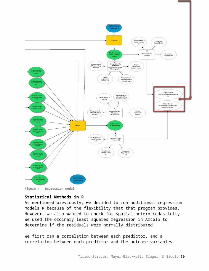
Our goals was to accurately predict the overall school STAR achievement in Language Arts ad overall school STAR achievement in Math at each school. We then aimed to compare the residuals from our model using spatial features with our model using only demographic data. First, we used summary statistics in ArcGIS to gain a better understanding of the range of our predictors. Next, we used the Ordinary Least Squares tool in ArcGIS to evaluate correlations and residuals.

Figure 4 - Regression model

Tirado-Strayer, Mayer-Blackwell, Siegel, & Biddle 7

Statistical Methods in RAs mentioned previously, we decided to run additional regression models R because of the flexibility that that program provides. However, we also wanted to check for spatial heteroscedasticity. We used the ordinary least squares regression in ArcGIS to determine if the residuals were normally distributed.

We first ran a correlation between each predictor, and a correlation between each predictor and the outcome variables. This allowed use to determine the effect that each predictor had on the outcome variable, and whether or not that effect was statistically significant. By also testing the correlations between each predictor, we were able to determine colinearities (for example, cold spots are negatively correlated with hot spots of the same variable). It was important to test for colinearity prior to running regressions so that we would not have redundant variables in our regression.

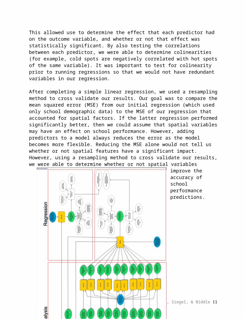
After completing a simple linear regression, we used a resampling method to cross validate our results. Our goal was to compare the mean squared error (MSE) from our initial regression (which used only school demographic data) to the MSE of our regression that accounted for spatial factors. If the latter regression performed significantly better, then we could assume that spatial variables may have an effect on school performance. However, adding predictors to a model always reduces the error as the model becomes more flexible. Reducing the MSE alone would not tell us whether or not spatial features have a significant impact. However, using a

resampling method to cross validate our results, we were able to determine whether or not spatial variables improve the accuracy of school performance predictions.

Tirado-Strayer, Mayer-Blackwell, Siegel, & Biddle 8

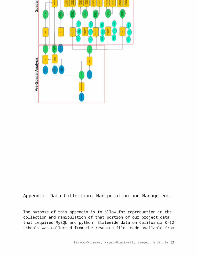
Appendix: Data Collection, Manipulation and Management.

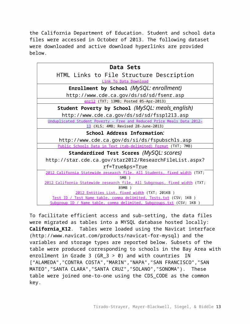
The purpose of this appendix is to allow for reproduction in the collection and manipulation of that portion of our project data that required MySQL and python. Statewide data on California K-12 schools was collected from the research files made available from the California Department of Education. Student and school data files were accessed in October of 2013. The following dataset were downloaded and active download hyperlinks are provided below.

Data SetsHTML Links to File Structure Description

Link To Data Download

Enrollment by School (MySQL: enrollment)

Tirado-Strayer, Mayer-Blackwell, Siegel, & Biddle 9

http://www.cde.ca.gov/ds/sd/sd/fsenr.aspenr12 (TXT; 13MB; Posted 05-Apr-2013)

Student Poverty by School (MySQL: meals_english)http://www.cde.ca.gov/ds/sd/sd/fssp1213.asp

Unduplicated Student Poverty – Free and Reduced Price Meals Data 2012 –13 (XLS; 4MB; Revised 28-June-2013)

School Address Information:http://www.cde.ca.gov/ds/si/ds/fspubschls.aspPublic Schools Data in Text (tab-delimited) Format (TXT; 7MB)

Standardized Test Scores (MySQL: scores)http://star.cde.ca.gov/star2012/ResearchFileList.aspx?rf=True&ps=True

2012 California Statewide research file, All Students, fixed width (TXT; 5MB )2012 California Statewide research file, All Subgroups, fixed width (TXT; 89MB )

2012 Entities List, fixed width (TXT; 201KB )Test ID / Test Name table, comma delimited, Tests.txt (CSV; 1KB )

Subgroup ID / Name table, comma delimited, Subgroups.txt (CSV; 1KB )

To facilitate efficient access and sub-setting, the data files were migrated as tables into a MYSQL database hosted locally: California_K12. Tables were loaded using the Navicat interface (http://www.navicat.com/products/navicat-for-mysql) and the variables and storage types are reported below. Subsets of the table were produced corresponding to schools in the Bay Area with enrollment in Grade 3 (GR_3 > 0) and with countries IN [“ALAMEDA","CONTRA COSTA","MARIN","NAPA","SAN FRANCISCO","SAN MATEO","SANTA CLARA","SANTA CRUZ","SOLANO","SONOMA"). These table were joined one-to-one using the CDS_CODE as the common key.

Tirado-Strayer, Mayer-Blackwell, Siegel, & Biddle 10

enrollment

+-----------+--------------+------+-----+---------+-------+| Field | Type | Null | Key | Default | Extra |+-----------+--------------+------+-----+---------+-------+| CDS_CODE | varchar(255) | YES | | NULL | || COUNTY | varchar(255) | YES | | NULL | || DISTRICT | varchar(255) | YES | | NULL | || SCHOOL | varchar(255) | YES | | NULL | || ETHNIC | int(11) | YES | | NULL | || GENDER | varchar(255) | YES | | NULL | || KDGN | int(11) | YES | | NULL | || GR_1 | int(11) | YES | | NULL | || GR_2 | int(11) | YES | | NULL | || GR_3 | int(11) | YES | | NULL | || GR_4 | int(11) | YES | | NULL | || GR_5 | int(11) | YES | | NULL | || GR_6 | int(11) | YES | | NULL | || GR_7 | int(11) | YES | | NULL | || GR_8 | int(11) | YES | | NULL | || UNGR_ELM | int(11) | YES | | NULL | || GR_9 | int(11) | YES | | NULL | || GR_10 | int(11) | YES | | NULL | || GR_11 | int(11) | YES | | NULL | || GR_12 | int(11) | YES | | NULL | || UNGR_SEC | int(11) | YES | | NULL | || ENR_TOTAL | int(11) | YES | | NULL | || ADULT | int(11) | YES | | NULL | |+-----------+--------------+------+-----+---------+-------+

scores

+---------------------------------------+--------------+------+-----+---------+-------+| Field | Type | Null | Key | Default | Extra |+---------------------------------------+--------------+------+-----+---------+-------+| CDS_CODE | varchar(50) | YES | | NULL | || County_Code | varchar(50) | YES | | NULL | || District_Code | varchar(50) | YES | | NULL | || School_Code | varchar(50) | YES | | NULL | || Charter_Number | varchar(50) | YES | | NULL | || Test_Year | varchar(50) | YES | | NULL | || Subgroup_ID | varchar(50) | YES | | NULL | || Test_Type | varchar(50) | YES | | NULL | || CAPA_Assessment_Level | varchar(50) | YES | | NULL | || Total_STAR_Enrollment | mediumint(9) | YES | | NULL | || Total_Tested_At_Entity_Level | mediumint(9) | YES | | NULL | || Total_Tested_At_Subgroup_Level | mediumint(9) | YES | | NULL | || Grade | tinyint(4) | YES | | NULL | || Test_Id | tinyint(4) | YES | | NULL | || STAR_Reported_EnrollmentCAPA_Eligible | mediumint(9) | YES | | NULL | || Students_Tested | mediumint(9) | YES | | NULL | || Percent_Tested | float | YES | | NULL | || Mean_Scale_Score | float | YES | | NULL | || Percentage_Advanced | float | YES | | NULL | || Percentage_Proficient | float | YES | | NULL | || Percentage_At_Or_Above_Proficient | float | YES | | NULL | || Percentage_Basic | float | YES | | NULL | || Percentage_Below_Basic | float | YES | | NULL | || Percentage_Far_Below_Basic | float | YES | | NULL | || Students_with_Scores | float | YES | | NULL | || CMASTS_Average_Percent_Correct | float | YES | | NULL | |+---------------------------------------+--------------+------+-----+---------+-------+

Tirado-Strayer, Mayer-Blackwell, Siegel, & Biddle 11

meals_english

+------------------------------+--------------+------+-----+---------+-------+| Field | Type | Null | Key | Default | Extra |+------------------------------+--------------+------+-----+---------+-------+| CDS_CODE | varchar(255) | YES | | NULL | || COUNTY_CODE | varchar(255) | YES | | NULL | || DISTRICT_CODE | varchar(255) | YES | | NULL | || SCHOOL_CODE | varchar(255) | YES | | NULL | || CHARTER_NUMBER | varchar(255) | YES | | NULL | || PROVISION_2_3 | varchar(255) | YES | | NULL | || DATA_ON_PROVISION | varchar(255) | YES | | NULL | || COUNTY | varchar(255) | YES | | NULL | || LEA | varchar(255) | YES | | NULL | || SCHOOL | varchar(255) | YES | | NULL | || LOW_GRADE | varchar(255) | YES | | NULL | || HIGH_GRADE | varchar(255) | YES | | NULL | || CALPADS_ENROLMENT | varchar(255) | YES | | NULL | || FREE_MEAL | varchar(255) | YES | | NULL | || PERECENT_FREE_MEAL | varchar(255) | YES | | NULL | || FREE_OR_REDUCED_MEAL | varchar(255) | YES | | NULL | || PERCENT_FREE_OR_REDUCED_MEAL | varchar(255) | YES | | NULL | |+------------------------------+--------------+------+-----+---------+-------+

Percentage of students in each self-declared ethnic category is not directly reported. This required calculation from enrollment counts divided by a school’s total enrollment. Enrollment counts by each self-reported category by school were extracted from the MySQL database and written to individual files, one for each ethnic group.

Code 0 = Not reportedCode 1 = American Indian or Alaska Native, Not HispanicCode 2 = Asian, Not HispanicCode 3 = Pacific Islander, Not HispanicCode 4 = Filipino, Not HispanicCode 5 = Hispanic or LatinoCode 6 = African American, not HispanicCode 7 = White, not Hispanic Code 9 = Two or More Races, Not Hispanic

Tirado-Strayer, Mayer-Blackwell, Siegel, & Biddle

mysql -h localhost -u root --local-infile –p

USE California_K12

CREATE TABLE bay_en_eth_1 SELECT CDS_CODE, COUNTY, SCHOOL, ETHNIC, sum(ENR_TOTAL) FROM enrollment WHERE COUNTY IN ("ALAMEDA","CONTRA COSTA","MARIN","NAPA","SAN FRANCISCO","SAN MATEO","SANTA CLARA","SANTA CRUZ","SOLANO","SONOMA") AND ETHNIC =1 GROUP BY CDS_CODE;

12

Schools were tracked by their CDS code (1st column). According to California Department of Education, “this 14-digit code is the official, unique identification each school within California. The first two digits identify the county. The next five digits identify the school district, and the last seven digits identify the school.” Percentages of students in each self-reported ethnic group were calculated from individual files using a custom python script compile.py:

Tirado-Strayer, Mayer-Blackwell, Siegel, & Biddle

compile.pyimport sysl = [1,2,3,4,5,6,7,8,9,"T"] # LIST OF ETHNIC CODESlf = ["bay_en_eth_1.txt","bay_en_eth_2.txt","bay_en_eth_3.txt","bay_en_eth_4.txt","bay_en_eth_5.txt","bay_en_eth_6.txt","bay_en_eth_7.txt","bay_en_eth_8.txt","bay_en_eth_9.txt","bay_enr_tot.txt"] # LIST OF INDIVIDUAL COUNT FILES

D = {}for eth,file in zip(l,lf): eth = str(eth) fh = open(file, 'r') for line in fh: if eth !="T": cds,county,school,ethnic, count = line.strip().split("\t") else: cds,county,school, count = line.strip().split("\t") count = int(count) if cds not in D.keys(): D[cds] = {"1":0,"2":0,"3":0,"4":0,"5":0,"6":0,"7":0,"8":0,"9":0, "T":0} else: D[cds][eth] = count fh.close()

Dp = {}for c in D.keys(): if c not in Dp.keys(): Dp[c] ={"1":float(5),"2":float(0),"3":float(0),"4":float(0),"5":float(0),"6":float(0),"7":float(0),"8":float(0),"9":float(0), "T":float(0)} for i in l[0:-1]: i = str(i) try: Dp[c][i] = float(D[c][i])/float(D[c]['T']) except ZeroDivisionError: Dp[c][i] = float(0)

for c in sorted(D.keys()): sys.stdout.write(c) for i in l[0:-1]: i = str(i) a = round(Dp[c][i],2) sys.stdout.write("\t"+str(a)) sys.stdout.write("\n")

Individual Files (example: bay_en_eth_1.txt)01100170109835 Alameda FAME Public Charter 1 1401100170112607 Alameda Envision Academy for Arts & Technology 1 401100170125567 Alameda Urban Montessori Charter 1 1

13

Using the CDS_CODE as foreign key, we joined these percentages to our BayArea_Elementary_Schools_Summary3.txt using the python script join.py:

The resulting file was BayArea_Elementary_Schools_Summary4.txt. Which was imported into ArcGIS and used for geocoding and subsequent analysis.

Tirado-Strayer, Mayer-Blackwell, Siegel, & Biddle

join.pyimport sysD= {}fh1 = open(sys.argv[1], 'r')fh2 = open(sys.argv[2],'r')for line in fh1: units = line.strip().split("\t") my_key = units[0] D[my_key] = line.strip()

for line in fh2: units = line.strip().split("\t") CDS = units[0].replace("'","") sys.stdout.write(line.strip() + "\t" + D[CDS] + "\n")

The resulting file bay_en_percentages.txt summarizes the percent of total enrollment in each ethnic category.

CDS_CODE ETH_NAT_AM ETH_ASIAN ETH_PAC_ISL ETH_FILIPINO ETH_LATINOETH_AFR_AM ETH_WHITE NULL ETH_TWO_RACES

01100170109835 0.0 0.19 0.02 0.03 0.13 0.09 0.52 0.0 0.001100170112607 0.0 0.02 0.01 0.0 0.37 0.47 0.05 0.0 0.0201100170118489 0.0 0.0 0.01 0.01 0.65 0.32 0.0 0.0 0.001100170123968 0.0 0.0 0.0 0.01 0.39 0.28 0.15 0.0 0.11

14