Greenhouse gas monitoring at the Zeppelin station, Ny ...
67
Greenhouse gas monitoring at the Zeppelin station, Ny-Ålesund, Svalbard, Norway Annual report 2003 Report: TA reference no.: ISBN no. Employer: Executing research institution: Authors: NILU OR 59/2004 TA-2042/2004 82-425-1610-3 Norwegian Pollution Control Authority (SFT) Norwegian Institute for Air Research (NILU) N. Schmidbauer, C. Lunder, O. Hermansen, F. Stordal, J. Schaug, I.T. Pedersen, K. Holmén, O.-A. Braathen (all NILU), J. Ström (Stockholm University) Greenhouse gas monitoring at the Zeppelin station, Ny-Ålesund, Svalbard, Norway Annual report 2003 Report 907/04
Transcript of Greenhouse gas monitoring at the Zeppelin station, Ny ...

Greenhouse gas monitoring at the Zeppelin station, Ny-Ålesund, Svalbard, Norway Annual report 2003
Report: TA reference no.: ISBN no. Employer: Executing research institution: Authors:
NILU OR 59/2004 TA-2042/2004 82-425-1610-3 Norwegian Pollution Control Authority (SFT) Norwegian Institute for Air Research (NILU) N. Schmidbauer, C. Lunder, O. Hermansen, F. Stordal, J. Schaug, I.T. Pedersen, K. Holmén, O.-A. Braathen (all NILU), J. Ström (Stockholm University)
Greenhouse gas monitoring at the Zeppelin station, Ny-Ålesund, Svalbard, Norway Annual report 2003
Report 907/04

Greenhouse gas monitoring at the Zeppelin station, Ny-Ålesund, Svalbard, Norway: Annual report 2003 - Annual report 2003 (TA-2042/2004)
2

Greenhouse gas monitoring at the Zeppelin station, Ny-Ålesund, Svalbard, Norway: Annual report 2003 - Annual report 2003 (TA-2042/2004)
3
Preface In 1999 the Norwegian Pollution Control Authority (SFT) and NILU signed a contract commissioning NILU to run a programme for monitoring greenhouse gases at the Zeppelin station, close to Ny-Ålesund at Svalbard. At the same time NILU started to coordinate a project funded by the European Commission called SOGE (System for Observation of halogenated Greenhouse gases in Europe) The funding from SFT enabled NILU to broadly extend the measurement programme and associated activities, making the Zeppelin station a major contributor of data on a global as well as a regional scale. The unique location together with the infrastructure of the scientific research community at Ny-Ålesund makes it a well suited platform for monitoring the global changes of ozone depleting substances (ODS) and greenhouse gases. The measurement programme includes a range of chlorofluorocarbons (CFC), hydrofluoro-carbons (HFC), hydrochlorofluorocarbons (HCFC), halones as well as other halogenated organic gases, sulphurhexafluoride (SF6), methane (CH4) and carbon monoxide (CO). The amount of particles in the air is measured by the use of an aethalometer and a Precision-Filter-Radiometer (PFR) sun photometer. The station is also basis for measurements of carbon dioxide (CO2) and particles performed by Stockholm University (SU). These activities are funded by the Swedish Environmental Protection Agency. Data from the monitoring activities are processed and used as input data in the work on international agreements like the Kyoto and the Montreal Protocols. This report summarises the activities and results of the climate monitoring programme during year 2003.

Greenhouse gas monitoring at the Zeppelin station, Ny-Ålesund, Svalbard, Norway: Annual report 2003 - Annual report 2003 (TA-2042/2004)
4

Greenhouse gas monitoring at the Zeppelin station, Ny-Ålesund, Svalbard, Norway: Annual report 2003 - Annual report 2003 (TA-2042/2004)
5
Contents
Preface....................................................................................................................................... 3
Summary ................................................................................................................................... 7
1. Greenhouse gases and aerosols ................................................................................. 9 1.1 Radiative forcing.......................................................................................................... 9 1.2 Natural greenhouse gases ............................................................................................. 9 1.3 Synthetic greenhouse gases........................................................................................ 10 1.4 Aerosols...................................................................................................................... 11
2. The Zeppelin station ................................................................................................ 12 2.1 Description of the station ........................................................................................... 12 2.2 Activities at the station............................................................................................... 13 2.2.1 NILU activities........................................................................................................... 13 2.2.2 Stockholm University (SU)........................................................................................ 13 2.2.3 NOAA ........................................................................................................................ 15 2.3 SOGE ......................................................................................................................... 15
3. Measurements........................................................................................................... 17 3.1 Instruments and methods............................................................................................ 17 3.1.1 Halocarbons................................................................................................................ 17 3.1.2 Methane...................................................................................................................... 19 3.1.3 Carbon Monoxide....................................................................................................... 22 3.1.4 Sun photometer measurements at Ny-Ålesund, Spitzbergen during 2003 ................ 23 3.2 Measurements ............................................................................................................ 26
4. Trends........................................................................................................................ 27 4.1 GC-MS in situ observations ....................................................................................... 27
5. Indirect methods for quantification of emissions .................................................. 34 5.1 General approach ....................................................................................................... 35 5.2 Emissions on a global scale........................................................................................ 35 5.3 Emissions on regional and country scales.................................................................. 37 5.3.1 Dispersion models ...................................................................................................... 37 5.3.2 Inverse modelling....................................................................................................... 41
6. Background information on Montreal and Kyoto Protocol................................. 43 6.1 The Montreal Protocol on substances that deplete the ozone layer ........................... 44 6.2 Amendments and Adjustments to the Protocol.......................................................... 45 6.2.1 London 1990 .............................................................................................................. 45 6.2.2 Copenhagen 1992....................................................................................................... 45 6.2.3 Vienna 1995 ............................................................................................................... 45 6.2.4 Montreal 1997 ............................................................................................................ 46 6.2.5 Beijing 1999 ............................................................................................................... 46 6.3 What might have happened without the Montreal Protocol?..................................... 46 6.4 Climate change and the Kyoto Protocol..................................................................... 47 6.5 In conclusion .............................................................................................................. 48

Greenhouse gas monitoring at the Zeppelin station, Ny-Ålesund, Svalbard, Norway: Annual report 2003 - Annual report 2003 (TA-2042/2004)
6
7. References ................................................................................................................. 49
8. Acknowledgement .................................................................................................... 51
Appendix A Measurement results ........................................................................................ 53

Greenhouse gas monitoring at the Zeppelin station, Ny-Ålesund, Svalbard, Norway: Annual report 2003 - Annual report 2003 (TA-2042/2004)
7
Summary This annual report describes the activities in the project Greenhouse gas monitoring at the Zeppelin station, year 2003. The report presents the Zeppelin monitoring station and some of the activities at the station, as well as current status for instruments and measurement methods used for climate gas monitoring. Results from the measurements are presented as monthly averages and plotted as daily averages. A wide range of anthropogenic as well as natural forcing mechanisms may lead to climate change. At present the known anthropogenic forcing mechanisms include well mixed greenhouse gases (carbon dioxide, nitrous oxide, methane, SF6 and halogenated hydrocarbons including CFCs, HFCs, HCFCs, halones and perfluorocarbons), ozone, aerosols (direct and indirect effects), water vapour and land surface albedo. In 1999 the Norwegian Pollution Control Authority (SFT) and NILU signed a contract commissioning NILU to run a programme for monitoring of climate gases at the Zeppelin station. The funding from SFT enables NILU to extend the greenhouse gas measurement programme and associated activities, making the Zeppelin station a major contributor of data on a global as well as a regional scale. The measurement programme at the Zeppelin station covers all major greenhouse gases - except N2O (due to lack of instrumentation). Measurements of greenhouse gases at the Zeppelin station are used together with data from other remote stations for monitoring of global changes as well as for assessment of regional emissions and tracing of emission sources. Results from the greenhouse gas monitoring are used for assessment of compliance with the Montreal and Kyoto Protocols. The Montreal Protocol, signed in 1987 and came into force in 1989, is a very flexible instrument, which has been adjusted several times in the following years. It is still of vital interest that the scientific community is continuing and even expanding efforts in atmospheric measurements and modelling in order to follow the process over the next decades. Vital inputs in models like the lifetimes, atmospheric trends, emissions of compounds are still undergoing continuous review processes and for example the lifetime of carbon tetrachloride was corrected with over 25 % during the last Scientific Assessment of Ozone Depletion in 2002 Climate Change and the Kyoto Protocol is a great environmental challenge to governments and the scientific community. Although there is superficial similarity between the topics of ozone depletion and those of climate change, and indeed much scientific interactions between the two, climate change has much wider implications. The range of materials and activities to be considered in regulations and the range of consequences are far larger and because of the long lifetime of carbon dioxide, the recovery from any effect on climate is far longer. There is a much larger gap to fill with both measurements and modelling. For Kyoto Protocol substances only a very limited number of measurement sites exist that can deliver high quality and high time-frequent measurements. For Europe the number of sites, which can be used by modellers, is still far below 10. The measurements at Ny-Ålesund are an important contribution for European emission modelling.

Greenhouse gas monitoring at the Zeppelin station, Ny-Ålesund, Svalbard, Norway: Annual report 2003 - Annual report 2003 (TA-2042/2004)
8
Measurements so far confirm the Zeppelin station's status as a global background station for climate gas monitoring. As the data series are expanded over time, they will make a good basis for investigations of global levels and trends. The first trend analysis of halogenated compounds based on three years data from Zeppelin are presented within this report The high frequency of data sampling enables studies of polluted air transport episodes. Combined with meteorological data and measurements from other European measurement stations, this is used for the investigation of regional emission inventories. The mean values for 2002 and 2003 presented in Table A follow the calculated long term trends. Carbon dioxide and methane slightly increasing, while the CFCs are about to level out or in case of CFC-11 decreasing, the HCFCs showing moderate increase rates, while the HFC concentrations in the atmosphere are still showing substantial yearly increase. Table A: Monthly mean concentration levels of climate gases at the Zeppelin station year 2003. All concentrations in pptv, except for methane (ppbv), carbon monoxide (ppbv), and carbon dioxide (ppmv).
Compound Mean 2002
Jan 2003
Feb 2003
Mar 2003
Apr 2003
May 2003
Jun 2003
Jul 2003
Aug 2003
Sep 2003
Oct 2003
Nov 2003
Dec 2003
Mean 2003
Methane 1813 1856 1851 1851 1839 1830 1810 1804 1810 1826 1842 1846 1861 1836 Carbon monoxide 126 161 175 178 170 149 128 102 103 119 126 138 150 141 Carbon dioxide* 374 381 381 377 371 366 367 374 379 382 375 Chlorofluorocarbons (CFC) CFC-11 267 267 264 264 264 264 261 260 260 261 CFC-12 562 561 559 565 564 563 565 567 563 561 563 565 564 CFC-113 82.0 83.3 82.7 82.9 83.0 82.9 82.8 83.3 82.8 82.8 CFC-114 18.2 17.9 17.4 17.8 17.5 17.5 17.7 17.0 17.5 17.4 17.4 17.2 17.3 CFC-115 8.60 8.62 8.48 8.51 8.42 8.48 8.57 8.61 8.67 8.68 8.57 Hydrofluorocarbons (HFC) HFC-125 2.55 3.54 3.36 3.26 3.26 3.20 3.58 3.56 3.74 3.72 3.42 HFC-134a 26.3 28.8 28.9 29.0 29.1 29.5 30.0 30.6 32.0 32.8 33.4 33.6 30.8 HFC-152a 3.40 3.87 4.07 4.18 4.24 4.18 3.86 4.20 4.52 4.83 4.12 Hydrochlorofluorocarbons (HCFC) HCFC-22 167 170 169 169 170 170 170 170 171 174 174 171 HCFC-123 1.06 1.14 1.19 1.27 1.16 1.16 1.09 1.00 0.96 0.97 0.89 1.00 HCFC-124 1.69 1.72 1.76 1.77 1.76 1.74 1.83 1.87 1.83 1.76 HCFC-141b 19.2 19.0 19.1 19.0 18.9 18.9 19.0 19.1 18.8 19.6 19.5 19.1 HCFC-142b 15.8 16.0 16.2 16.2 16.4 16.3 16.4 16.6 16.5 16.6 16.9 16.8 16.5 Halons H-1301 3.16 3.26 3.31 3.30 3.31 3.39 3.25 3.25 3.29 3.28 3.27 H-1211 4.52 4.58 4.55 4.56 4.59 4.60 4.51 4.56 4.60 4.61 4.56 Halogenated compounds Methylchloride 521 533 546 556 566 561 544 514 461 473 499 510 520 Methylbromide 9.40 8.64 8.44 8.68 8.63 8.48 8.00 7.83 8.64 8.85 8.47 Methyliodide 0.90 0.56 0.32 0.42 0.73 0.91 0.92 0.99 0.59 0.95 0.92 0.64 0.69 Methylendichloride 30.1 34.2 35.7 37.1 37.8 36.5 32.7 29.9 24.5 27.0 28.6 33.0 32.0 Chloroform 11.1 11.9 12.0 11.9 11.5 10.7 10.0 10.2 11.5 12.4 12.3 11.4 Methylchloroform 32.4 30.1 29.8 29.9 29.7 29.5 30.0 29.9 27.0 24.8 24.6 28.2 Carbontetrachloride 94.0 95.9 92.7 88.9 95.0 96.9 103.1 105.5 102.7 86.4 96.7 Perchloroethylene 4.20 4.40 5.95 4.28 3.20 4.26 3.99 3.69 2.85 3.61 4.20 4.14 3.95 Sulphurhexafluoride 5.0 5.0 5.0 5.0 5.1 5.2 5.2 5.2 4.9 5.0 5.1 5.1 5.1
*Measurements of CO2 performed by SU.

Greenhouse gas monitoring at the Zeppelin station, Ny-Ålesund, Svalbard, Norway: Annual report 2003 - Annual report 2003 (TA-2042/2004)
9
1. Greenhouse gases and aerosols
1.1 Radiative forcing
Changes in climate are caused by internal variability within the climate system and external factors, natural and anthropogenic. The effect can be described through the effect on radiative forcing caused by each factor. Increasing concentrations of greenhouse gases tends to increase radiative forcing, hence contributing to a warmer global surface, while some types of aerosols have the opposite effect. Natural factors such as changes in solar output or explosive volcanic activities will also influence on radiative forcing. Changes in radiative forcing, relative to pre industrial time, are indicated in Figure 1.
Figure 1: Known factors and their influence on radiative forcing relative to pre industrial time. The vertical lines indicate the uncertainties for each factor. (Source: IPCC.)
1.2 Natural greenhouse gases
Some gases in the atmosphere absorb the infrared radiation emitted by the Earth and emit infrared radiation upward and downward, hence raising the temperature near the Earth’s surface. These gases are called greenhouse gases. Some of these gases have large natural sources, like carbon dioxide (CO2), methane (CH4) and nitrous oxide (N2O). They have sustained a stable atmospheric abundance for the centuries prior to the industrial revolution. Emissions due to human activities have caused large increases in their concentration levels over the last century (figure 2), adding to radiative forcing. The atmospheric concentration of CO2 has increased by 30% since 1750. The rate of increase has been about 1.5 ppm (0.4%) per year over the last two decades. About three quarters of the anthropogenic emissions to the atmosphere is due to fossil fuel burning, the rest is mainly due to land-use change, especially deforestation.

Greenhouse gas monitoring at the Zeppelin station, Ny-Ålesund, Svalbard, Norway: Annual report 2003 - Annual report 2003 (TA-2042/2004)
10
The atmospheric concentration of CH4 has increased by 1060 ppb (150%) since 1750 and continues to increase. More than half of the current emissions are anthropogenic; use of fossil fuel, cattle, rice plants and landfills. Carbon monoxide (CO) emissions have been identified as a cause of increasing CH4 concentration. This is caused by CO reacting with reactive OH, thus preventing OH from reacting with CH4, a primary loss reaction for methane (ref. Daniel, Solomon). The atmospheric concentration of N2O has increased by 45 ppb (17%) since 1750 and continues to increase. About a third of the emissions are anthropogenic; agriculture, cattle feed lots and chemical industry.
Climate gases, historic trends
250
300
350
400
1000 1200 1400 1600 1800 2000Year
CO
2 ppm
/ N
2O p
pb
600
1000
1400
1800
CH
4 ppb
Nitrous oxide
Carbon dioxide
Methane
Figure 2: Changes in concentration levels over time for some natural climate gases.
Ozone (O3) is a reactive gas with relatively large variation in concentration levels. The amount of tropospheric O3 has increased by 35% since 1750, mainly due to anthropogenic emissions of O3-forming gases like volatile organic compounds (VOCs), carbon monoxide (CO) and nitrogen oxides. O3 forcing varies considerably by region and responds more quickly to changes in emissions than more long-lived greenhouse gases. Water vapour in the lower stratosphere is an effective greenhouse gas. The amount of water vapour is temperature dependent, increasing with higher temperatures. Another source of H2O is the oxidation of CH4 and possibly future direct injection of H2O from high-flying aircrafts. 1.3 Synthetic greenhouse gases
Another class of gases are the man made greenhouse gases, such as CFCs, HCFCs, HFCs PFCs, SF6 and halons. These gases did not exist in the atmosphere before the 20th century. Although these gases have much lower concentration levels than the natural gases mentioned above, they are strong infrared absorbers, many of them with extremely long atmospheric lifetimes resulting in high global warming potentials (Table 1). Some of these gases are ozone depleting, and they are regulated by the Montreal protocol. Concentrations of these gases are increasing more slowly than before 1995, some of them are decreasing. Their substitutes, however, mainly HFCs, and other synthetic greenhouse gases are currently increasing.

Greenhouse gas monitoring at the Zeppelin station, Ny-Ålesund, Svalbard, Norway: Annual report 2003 - Annual report 2003 (TA-2042/2004)
11
Table 1: Halocarbons measured at Ny-Ålesund and their relevance to the Montreal and Kyoto Protocols.
Species Chemical structure
Lifetime (years)
GWP1 Trend
Montreal or Kyoto Protocol
Comments on use
Chlorofluorocarbons (CFCs) F-11 CCl3F 45 4600 →↓ M phased out foam blowing, aerosol propellent F-12 CCl2F2 100 10600 →↓ M phased out temperature control
F-113 CCl2FCClF2 85 6000 →↓ M phased out solvent, electronics industry F-114 CClF2CClF2 300 9800 →↓ M phased out
F-115 CF3CClF2 1700 7200 →↓ M phased out Hydrochlorofluorocarbons (HCFCs) F-22 CHClF2 12 1700 ↑ M freeze temperature control, foam blowing
F-124 CF3CHClF 6 405 → M freeze temperature control F-141b CH3CFCl2 9 700 ↑ M freeze foam blowing, solvent
F-142b CH3CF2Cl 19 2400 ↑ M freeze foam blowing Hydrofluorocarbons (HFCs) F-125 C2HF5 29 3400 ↑ K temperature control F-134a CH2FCF3 14 1300 ↑ K temperature control, foam blowing,
solvent , aerosol propellent F-152a C2H4F2 1.4 120 ↑ K foam blowing
Halons F-1211 CBrClF2 11 1300 → M phased out fire extinguishing
F-1301 CBrF3 65 6900 → M phased out fire extinguishing Perfluorinated compounds (PFCs)
Sulfur hexafluoride SF6 3200 22200 →↑ K Mg-production,electronics industry Hexafluoro ethane C2F6 10000 11900 →↑ K Al-production,electronics industry
Other halogenated hydrocarbons Trichloroethane (Methyl chloroform)
CH3CCl3 5 140 ↓↓ M phased out solvent
Tetrachloro methane CCl4 35 1800 →↓ M phased out solvent
Methyl chloride CH3Cl 1.5 (→↓) natural emissions (algae) Dichloro methane CH2Cl2 0.5 9 →↓ solvent
Chloroform CHCl3 0.5 4 →↓ solvent
Trichloro ethylene CCl2CHCl →↓ solvent Perchloro ethylene C2Cl4 →↓ solvent
Methyl bromide CH3Cl 1.2 →↓ M freeze: 1995
agriculture, natural emissions (algae)
Methyl iodide CH3I → natural emissions
1GWP(Global warming potensial) 100 years time periode, CO2 = 1 1.4 Aerosols
Major sources of anthropogenic aerosols are fossil fuel and biomass burning. Aerosols like sulphate, biomass burning aerosols and fossil fuel organic carbon produce negative radiative forcing, while fossil fuel black carbon has a positive radiative effect. Aerosols vary considerably by region and respond quickly to changes in emissions. Natural aerosols like sea salt, dust and sulphate and carbon aerosols from natural emissions are expected to increase as a result of climate change. In addition to their direct radiative forcing, aerosols have an indirect radiative forcing through their effect on cloud formation.

Greenhouse gas monitoring at the Zeppelin station, Ny-Ålesund, Svalbard, Norway: Annual report 2003 - Annual report 2003 (TA-2042/2004)
12
2. The Zeppelin station
2.1 Description of the station
The monitoring station is located on the Zeppelin Mountain, close to Ny-Ålesund at Svalbard. At 79° north the station is placed in an undisturbed arctic environment, away from major pollution sources. Situated 474 meters asl and most of the time above the inversion layer, there is minimal influence from local pollution sources in the nearby small community of Ny-Ålesund.
Figure 3: The monitoring station is located at the Zeppelin Mountain 474 meters asl.
The Zeppelin station is owned and maintained by the Norwegian Polar Institute. NILU is responsible for the scientific activities at the station. The station was built in 1989-1990. After 10 years of use, the old building was no longer sufficient for operation of advanced equipment and the increasing amount of activities. The old building was removed to give place to a new modern station that was opened in May 2000. The new monitoring station was realised by funds from the Norwegian Ministry of Environment and the Wallenberg Institution via Stockholm University (SU). The station building was constructed using selected materials to minimise contamination and influence on any ongoing measurements. All indoor air is ventilated away down from the mountain. The building contains several separate laboratories, some for permanent use by NILU and SU, others intended for short-term use like measurement campaigns and visiting scientists. A permanent data communication line permits on-line contact with the station for data reading and instrument control.

Greenhouse gas monitoring at the Zeppelin station, Ny-Ålesund, Svalbard, Norway: Annual report 2003 - Annual report 2003 (TA-2042/2004)
13
The unique location of the station makes it an ideal platform for the monitoring of global atmospheric change. The measurement activities at the Zeppelin station contributes to a number of global, regional and national monitoring networks:
• SOGE (System for Observation of halogenated Greenhouse Gases in Europe) • AGAGE (Advanced Global Atmospheric Gases Experiment) • EMEP (European Monitoring and Evaluation Programme under "UN Economic
Commission for Europe") • Network for detection of stratospheric change (NDSC under UNEP and WMO) • Global Atmospheric Watch (GAW under WMO) • Arctic Monitoring and Assessment Programme (AMAP)
2.2 Activities at the station
2.2.1 NILU activities The main goals of NILU’s research activities at the Zeppelin station are:
• Studies of climate related matters and stratospheric ozone • Exploration of atmospheric long range transport of pollutants • Characterization of the arctic atmosphere and studies of atmospheric processes and
changes NILU performs measurements of halogenated greenhouse gases as well as methane and carbon monoxide using automated gas chromatographs with high sampling frequencies. A mass spectrometric detector is used to determine more than 30 halogenated compounds, automatically sampled 6 times per day. Methane and CO are sampled 3 times per hour. This high sampling frequency gives valuable data for the examination of episodes caused by long-range transport of pollutants as well as a good basis for the study of trends and global atmospheric change. Close cooperation with SOGE-partners on the halocarbon instrument and audits on the methane and CO-instruments (performed by EMPA on the behalf of GAW/WMO) show that the instruments deliver data of high quality. The amount of particles in the air are monitored by a continuous aethalometer and by the use of a Precision-Filter-Radiometer (PFR) sun photometer. The aethalometer measures the total amount of particles at ground level, while the sun photometer measures the amount and size distribution through a total column. The station at Zeppelin Mountain is also used for a long range of measurements, which are not directly related to climate gas monitoring, including daily measurements of sulphur and nitrogen compounds (SO2, SO4
2-, (NO3- + HNO3) and (NH4
+ + NH3), main compounds in precipitation, mercury, persistent organic pollutants (HCB, HCH, PCB, DDT, PAH etc.), as well as tropospheric and stratospheric ozone. 2.2.2 Stockholm University (SU) At the Zeppelin station carbon dioxide (CO2) and atmospheric particles are measured by Stockholm University (Institute of Applied Environmental Research, ITM).

Greenhouse gas monitoring at the Zeppelin station, Ny-Ålesund, Svalbard, Norway: Annual report 2003 - Annual report 2003 (TA-2042/2004)
14
SU maintains a continuous infrared CO2 instrument, which has been monitoring since 1989. The continuous data are enhanced by the weekly flask sampling programme in co-operation with NOAA CMDL. Analysis of the flask samples provide CH4, CO, H2, N2O and SF6 data for the Zeppelin station. The CO2 monitoring project at the Zeppelin station has three goals:
• Provide a baseline measurement of European Arctic CO2 concentrations. • Allow detailed analysis of the processes behind CO2 variations in the Arctic on time-
scales from minutes to decades. • Understand how human activities and climate change perturb the global carbon cycle
and thus give variations of atmospheric CO2 and CH4. SU has several instruments at Zeppelin station, which measure particles in the atmosphere. Aerosol particles tend to reflect light and can therefore alter the Earth’s radiation balance. The Optical Particle Counter (OPC) gives the concentration of aerosol particles and, combined with data from the Nephelometer, clues to the particles’ age and origin. Size distribution is acquired from a Differential Mobility Analyser (DMA). Understanding atmospheric chemical processes requires more than just CO2 and aerosols and scattering data. A total filter allows creating a bi-daily record of the chemical composition of aerosol particles.
Figure 4: SU has been measuring CO2 at Mt. Zeppelin since 1989.

Greenhouse gas monitoring at the Zeppelin station, Ny-Ålesund, Svalbard, Norway: Annual report 2003 - Annual report 2003 (TA-2042/2004)
15
2.2.3 NOAA NOAA CMDL (The Climate Monitoring and Diagnostics Laboratory at The National Oceanic and Atmospheric Administration in USA) operates a global air sampling network. The Zeppelin station is included in this network (Figure 5). Air is sampled on a weekly basis in glass canisters and shipped to the laboratories at Boulder, Colorado (USA). The measurement programme includes CH4, CO, H2, N2O and SF6. Results from the analysis are used in studies of trends, seasonal variations and global distribution of greenhouse gases.
CMDL observatoryHalocarbon air samplingCarbon cycle air samplingCarbon cycle tower measurementsCarbon cycle aircraft samplingAircraft measurements
Easter Island
South PoleHalley Bay
FortalezaSantarem
Barbados
Key Biscayne
Island
Palmer Station
Christmas Island
Niwot Ridge
WLEFUtah
MidwayIsland
PointArena
Shemya
Cold Bay Poker Flats
Barrow
American Samoa
Rarotonga
Pacific Ocean Cruises
Baring HeadTierra Del Fuego
Mauna Loa
Carr
Harvest Forest
Summit
Alert
Bermuda
KWKT
Cape Grim
Syowa
Crozet
Seychelles
Azores
Tenerife
Mace Head
Baltikum
Polarfront
Zeppelin
Negev desert
Romania
Namibia
AscensionIsland
MaldivesGuam
Tae-Ahn Pen.
MongoliaKazakstan
Hungary
AlgeriaMalta
Figure 5: NOAA’s global air sampling network.
2.3 SOGE
SOGE is an integrated system for observation of halogenated greenhouse gases in Europe. SOGE builds on a combination of observations and modelling. High resolution in situ observation at four background stations forms the backbone of SOGE. A network is being developed between the four stations. This includes full inter-calibration and common quality control, which is adopted from the global monitoring network of Advanced Global Atmospheric Gases Experiment (AGAGE). The in situ measurements will be combined with vertical column measurements, which have been made at two of the network sites for up to about 15 years, as a part of Network for Detection of Stratospheric Change (NDSC). One purpose of this combination is determination of trends in the concentrations of the gases under consideration. Integration of the observations with a variety of model tools will allow extensive and original exploitation of the data. The integrated system will be used to verify emissions of the measured substances in Europe down to a regional scale. This will be obtained by the use of a model labelling air-parcels with their location and time of origin, so it is possible to identify the various sources that contribute to the concentrations measured at the network sites. The results will contribute

Greenhouse gas monitoring at the Zeppelin station, Ny-Ålesund, Svalbard, Norway: Annual report 2003 - Annual report 2003 (TA-2042/2004)
16
to the assessment of compliance with the Kyoto and Montreal protocols, and they will be utilised also to define criteria for future monitoring of halocarbons in Europe. Global models are used to estimate impacts of the observed compounds on climate change and the ozone layer. The impacts will be evaluated in terms of radiative forcing and Global Warming Potential (GWP), and ozone destruction and Ozone Depletion Potential (ODP), respectively. SOGE is funded by European Commission Directorate General Research 5th Framework Programme Energy, Environment and Sustainable Development.
Figure 6: The SOGE climate gas monitoring stations.
Mt Zeppelin
Mace Head
Jungfraujoch
Mt Cimone
SOGE stations
Mt. Zeppelin Svalbard, Norway 78º54’ N, 11º53’ E 475 m asl
Mace Head
Ireland 53º20’ N, 9º54’ W 14 m asl
Jungfraujoch
Switzerland 46º32’ N, 7º59’ E 3500 m asl
Mt. Cimone
Italy 44º12’ N, 10º42’ E 2165 m asl

Greenhouse gas monitoring at the Zeppelin station, Ny-Ålesund, Svalbard, Norway: Annual report 2003 - Annual report 2003 (TA-2042/2004)
17
3. Measurements
3.1 Instruments and methods
3.1.1 Halocarbons To perform long-term high quality observations of volatile halocarbons at the Zeppelin station a specially designed instrument was installed in late spring 2000. The instrument currently monitors more than 20 compounds, including CFCs, HFCs, HCFCs, Halons and a range of other halogenated species. The gases monitored by the instrument are listed together with CH4, CO and CO2 in Table 1. The instrument is a fully automated adsorption/desorption sampling device (ADS) coupled with an automatic gas chromatograph with a mass spectrometric detector (GC-MS). The system provides 6 air samples during 24 hours. The instrument is the same instrument as the ones located at the SOGE stations Mace Head and Jungfraujoch and all the five AGAGE sites. The four sites within the SOGE project are using calibration tanks, which are pressurized simultaneously at Mace Head and then calibrated to AGAGE (Advanced Global Atmospheric Gases Experiment) scale. The instrument is remote controlled from NILU, but there is a daily inspection at the site from personnel from the Norwegian Polar Institute. There are about 4 to 6 visits from NILU each year for major maintenance work. All data are transferred to NILU on a daily basis. All data are processed by software, which is common for all AGAGE and SOGE stations. Hard disc crash in January, lack of calibration gas in beginning of April, bad instrument performance in July – September due to leak problems and broken turbo pump in the MS and broken water trap in November, resulted in data losses in these periods. In consideration of these periods of data losses, the overall data coverage is considered to be good for the year 2003. As member of the SOGE network and due to the good quality of data produced, the Zeppelin station is accepted as an associated member of the AGAGE network. Results from the outlined trending methods are illustrated in Figure 7 for HFC-134a for Zeppelin (2001-2003) where the panels show (a) The raw observed GC-MS data, (b) the baseline filtered data with trend curve and filter, (c) the algorithm derived growth rate in pptv/year and (d) %/year. Note that the annual yearly growth rate is not shown in this data, just the filtering results from the data using the 650-day smoothing after filtering of the seasonal cycle. The averaged seasonal cycle for HFC-134a for Zeppelin is shown in Figure 8. For more about trends and results go to Chapter 4 and Appendix.

Greenhouse gas monitoring at the Zeppelin station, Ny-Ålesund, Svalbard, Norway: Annual report 2003 - Annual report 2003 (TA-2042/2004)
18
1998 1999 2000 2001 2002 2003 2004 2005
1998 1999 2000 2001 2002 2003 2004 2005
1998 1999 2000 2001 2002 2003 2004 2005
Figure 7: Generation of trends in HFC-134a from observations at Zeppelin for 2001-2003. See text for panel description. Reproduced with permission, P.B. Krummel, CSIRO, Australia.

Greenhouse gas monitoring at the Zeppelin station, Ny-Ålesund, Svalbard, Norway: Annual report 2003 - Annual report 2003 (TA-2042/2004)
19
Figure 8: Annually averaged (2001-2003) seasonal cycle for HFC-134a from GC-MS observations at Zeppelin. Reproduced with permission, P.B. Krummel, (CSIRO).
3.1.2 Methane CH4 is the second most significant greenhouse gas, and its level has been increasing since the beginning of the 19th century. Global mean concentrations reflect an annual increase, and the annual averaged concentration was 1782 ppb in 2001. The annual concentrations produce a peak in the northernmost latitudes and decrease toward the southernmost latitudes, suggesting significant net sources in northern latitudes. The global growth rate is 8 ppb/year on average for the period 1984-2001, but the rates show a distinct decrease from the 1980s to 1990s. Growth rates decreased significantly in some years, including 1992, when negative values were recorded in northern high latitudes, and 1996, when growth almost stopped in many regions. However, both hemispheres experienced high growth rates in 1998, caused by an exceptionally high global mean temperature. And the global growth rates decreased again largely to record negative values in 2000 for the first time during the analysis period. Monthly mean concentrations have a seasonal variation with high concentrations in winter and low ones in summer. Unlike CO2 , amplitudes of the seasonal cycle are large for CH4 not only in the Northern Hemisphere but also in southern high and mid-latitudes. In southern low latitudes, a distinct semi-annual component with a secondary maximum in boreal winter overlays the annual component. This is attributed to the large-scale transport of CH4 from the Northern Hemisphere (GAW homepage). At Mt. Zeppelin methane is monitored by the use of an automatic gas chromatograph with a flame ionisation detector (GC/FID). Air is sampled three times an hour and calibrated against an air standard once an hour. The instrument produces a large amount of data requiring a specially made system for the extensive data handling. The installation of new data collection equipment was the first step to enable the methane data being processed by the same system as the halocarbon data. This data system is specially made at the Scripps Institution of Oceanography in California, but needs an upgrade before it can include the methane measurements. All methane data will be recalculated when this system is in place. The instrument is quite old and there have been some problems with valve switching, detector function and the computer collecting the data, resulting in small periods of reduced data

Greenhouse gas monitoring at the Zeppelin station, Ny-Ålesund, Svalbard, Norway: Annual report 2003 - Annual report 2003 (TA-2042/2004)
20
availability. In consideration of these periods of data losses, the overall data coverage is considered to be good for the year 2003. It is expected that an almost complete data series can be recovered when transferred to the new data system. The instrument is calibrated against new traceable standards with references to standards used under the AGAGE programme. The last major audit was performed in September 2001 by personnel from the Swiss Federal Laboratories for Materials Testing and Research (EMPA) which is assigned by the World Meteorological Organization’s (WMO) to operate the Global Atmospheric Watch (GAW) World Calibration Center for Surface Ozone, Carbon Monoxide and Methane. The results are published in EMPA-WCC report 01/3, concluding that methane measurements at the Zeppelin station can be considered to be traceable to the GAW reference standard. A new major audit will be performed in 2005. The continuous data are enhanced by the weekly flask sampling programme performed by NOAA CMDL. Figure 9 shows nice correlation between the flask samples and the in situ measurements, both in seasonal variation and pollution events.
Zeppelin Daily 1998-2003
1700
17201740
1760
17801800
18201840
1860
18801900
1920
19401960
19802000
07.98 07.99 07.00 07.01 07.02 07.03
Date (mm.yy)
Met
hane
(ppb
v)
Figure 9: Methane measurements at Mt. Zeppelin 1998 – 2003. Weekly flask samples (red dots) performed by CMDL compared with daily averaged in situ measurements (black line) performed by NILU.
All the flask data for Zeppelin and the daily mean of all data are plotted in Figure 10 together with a fitted harmonic function. The blue function fitted to the flask data (red stars) has a gradient (methane concentration increase rate) of 3.63 ppb/year and crosses the y-axis in –5428 (i.e. x=0). The green function fitted to the daily mean data from Zeppelin (light blue cross) has a gradient of 3,21 and crosses the y-axis in –4609. The global growth rate of methane, determined using the measurements from the NOAA CMDL cooperative air sampling network, has since 2002 been between 1 and 5. The difference of the two curves is not constant, but in the region where they overlap, it is around 20 ppb. This system difference is comparable to other sites where both continuous and flask data are collected. Compared to the harmonic function fitted to the data (Figure 11), there are 41 peaks that deviate more than 20 ppb from the function. In addition, in the period 1.4 –22.5 2002 the GC measurements are systematically lower than the function, and in the period 13.4-8.6 2003 the measurements are systematically higher than the function without crossing it. In the first period there is a deviation in the continuous data from the flask measurements, which we have not been able to

Greenhouse gas monitoring at the Zeppelin station, Ny-Ålesund, Svalbard, Norway: Annual report 2003 - Annual report 2003 (TA-2042/2004)
21
explain. In the second period the continuous data are consistent with the flask measurements. The form of the harmonic function can be an artefact of the first period hence creating the deviation also in the second.
Figure 10: Zeppelin flask data (red stars) with harmonic function (blue) together with GC daily mean data (light blue) with harmonic function (green) from year 1990 to 2010.
Figure 11: Zeppelin GC data (green line) with harmonic function (blue) from 2001 to 2004.

Greenhouse gas monitoring at the Zeppelin station, Ny-Ålesund, Svalbard, Norway: Annual report 2003 - Annual report 2003 (TA-2042/2004)
22
When more data have been collected in a year, we expect to have a sufficient time series to allow fitting the harmonic function whist dropping the suspect data in April-May 2002. Year to year shifts in increase rates should then also be possible to extract from the record. 3.1.3 Carbon Monoxide Tropospheric carbon monoxide CO is not a significant greenhouse gas, but brings about changes in the concentrations of greenhouse gases by interacting with hydroxyl radicals (OH). Concentrations of CO have increased in northern high latitudes since the mid-19th century, but have not changed significantly over Antarctica during the previous two millennia. The annual averaged concentration was about 93 ppb in 2001. The annual mean concentration is high in the Northern Hemisphere and low in the Southern Hemisphere, suggesting substantial anthropogenic emissions in the Northern Hemisphere. Though the level of CO was increasing before the mid-1980s, the averaged global growth rate was -0.8 ppb/year for the period from 1992 to 2001. The variability of the growth rates is large. High positive growth rates and subsequent high negative growth rates were observed in northern latitudes and southern low latitudes from 1997 to 1999. Monthly mean concentrations show a seasonal variation with large amplitudes in the Northern Hemisphere and small ones in the Southern Hemisphere. This seasonal cycle is driven by variations in OH concentration as a sink, emission by industries and biomass burning, and transportation on a large scale (GAW homepage). CO is closely liked to the cycles of methane and ozone and like methane plays a key role in the control of the OH radical. Its emissions have influence on the increasing tropospheric ozone and methane concentrations. The CO instrument at the Zeppelin station was reinstalled in September 2001. An inter-national calibration during an audit from Swiss Federal Laboratories for Material Testing and Research (EMPA) was performed the same month to assess the quality of the measurements. EMPA represented the Global Atmosphere Watch (GAW) programme to include the measurements on the Zeppelin Mountain in the GAW programme. The results are published in EMPA-WCC report 01/3, concluding that methane measurements at the Zeppelin station can be considered to be traceable to the GAW reference standard. The instrument is an automatic gas chromatograph with mercury oxide reduction followed by UV detection. It is performing analysis of 5 air samples and one standard within a time period of 2 hours. The standards are calibrated directly to a Scott-Marine Certificated standard and the Mace Head standards, which are related to the AGAGE-scale. The instrument has been running without serious interruptions since installation. Only small breaks with power fail on sample pump and hard disk crash on the computer collecting the data. The instrument uses the same system for data collection as the methane instrument. The overall data coverage is considered to be good for the year 2003. The continuous data are enhanced by the weekly flask sampling programme performed by NOAA CMDL. Figure 12 shows nice correlation between the flask samples and the in situ measurements, both in seasonal variation and pollution events (e.g. Dec. 2002).

Greenhouse gas monitoring at the Zeppelin station, Ny-Ålesund, Svalbard, Norway: Annual report 2003 - Annual report 2003 (TA-2042/2004)
23
CO, Mt. Zeppelin
0
50
100
150
200
250
10.00 04.01 11.01 05.02 12.02 06.03 01.04 08.04
Date
ppb v NILU
CMDL - flask
Figure 12: CO measurements at Mt. Zeppelin 2001 – 2003. Weekly flask samples performed by CMDL compared with hourly in situ measurements performed by NILU.
3.1.4 Sun photometer measurements at Ny-Ålesund, Spitzbergen during 2003 The sun photometer at Ny-Ålesund is a precision-filter-radiometer that accurately measures the direct sun radiation in four narrow spectral bands at 862, 500, 412, and 368 nm. The aerosol optical depth (AOD) can be determined from the measurements through a set of algorithms. The instrument is calibrated every year at the Physikalisch-Meteorologisches Observatorium Davos, World Radiation Center, (PMOD/WRC) by comparison with standard instruments that are calibrated at high altitude sites like Jungfraujoch or Mauna Loa. The main application of the instrument is to provide high quality spectral irradiance data to determine the AOD for the World Meteorological Organization, Global Atmosphere Watch (WMO GAW) programme in a small network of 12 stations established worldwide to test and demonstrate the feasibility of this concept and the methods. A sun tracker directs the photometer to the sun disc and leads the spectrometer to follow the sun across the sky during the day. The sun photometer is a passive remote sensing instrument that records the sun irradiance only, and it cannot carry out measurements during dark hours or during foggy or cloudy conditions. Fog and low clouds often occur in Ny-Ålesund, and this reduces the data completeness seriously. In 2002 and 2003, the instrument had a clear line-of-sight to the Sun during 13% of the time when the Sun was above the mathematical horizon. A relocation of the instrument at the Zeppelin mountain station (474 m asl) would give more results since the fog in this case often will be lower than the instrument, and the instrument could have a longer active period not being in the shade of surrounding mountains. So far, however, no sun tracker is available at the Zeppelin station. 2003 was not a good year with respect to data completeness since technical problems occurred in addition to fog and clouds conditions. The instrument temperature sensor failed in April, and the pointing of the sun photometer to the sun disc fell frequently out of range from May to July causing a loss of data. The requirement to data completeness was set rather strict

Greenhouse gas monitoring at the Zeppelin station, Ny-Ålesund, Svalbard, Norway: Annual report 2003 - Annual report 2003 (TA-2042/2004)
24
below; two 3-hour periods with 45 values each was needed in order to have a valid daily average a specific day. A reporting to EMEP applying a more tight cloud and tracking filtered data set than used here, and with comparison of the Ny-Ålesund 2003 data with corresponding results from Jungfraujoch in Switzerland and Hohenpeissenberg in Germany has also been given (Schaug and Wehrli, 2004). Figure 13 shows the AOD measured at Ny-Ålesund from the middle of April to the beginning of October. The Figure also gives the aerosol sulphate concentrations as measured at the Zeppelin mountain (475 m asl ) for comparison. The high aerosol load during spring and during winter that gives high AOD values and high aerosol sulphate concentrations compared to the summer measurements is typical. The arctic haze phenomenon has been observed for more than fifty years. Aircraft measurements revealed that most of the wintertime arctic haze was found in the boundary layer, but that distinct layers of haze also could be found at different altitudes up to 5 km (Ottar et al., 1986). There are strong inversions during winter that inhibits the exchange of air between the layers and prevents the formation of precipitation giving clouds. Removal mechanisms are therefore suppressed during winter and spring, and the cold and stable winter arctic boundary layer may extend into the industrial sources in the south. In summer precipitation occurs resulting in a fast removal of aerosols as well as water-soluble gases. The arctic haze is very well described by AMAP (1998) in their assessment report that additionally give a large number of references to related topics.
0.00
0.05
0.10
0.15
0.20
0.25
0.30
0.35
20-Apr-
03
27-A
pr-03
4-May
-03
11-M
ay-03
18-M
ay-03
25-M
ay-03
1-Jun
-03
8-Jun-0
3
15-Ju
n-03
22-Ju
n-03
29-Jun
-03
6-Jul-0
3
13-Ju
l-03
20-Ju
l-03
27-Ju
l-03
3-Aug
-03
10-A
ug-03
17-Aug
-03
24-A
ug-03
31-A
ug-03
7-Sep
-03
14-S
ep-03
Date
AO
D, d
aily
ave
rage
s
0
0.1
0.2
0.3
0.4
0.5
0.6
0.7
0.8
0.9
Aer
osol
sul
phat
e co
nc.,
daily
ave
rage
, in
ug
S/m
3
midAOD-863midAOD-501midAOD-412midAOD-368SO4 aero
Figure 13. Daily AOD averages at 368, 412, 501, and 863 nm measured in Ny Ålesund, and daily averages of sulphate concentrations in airborne particles measured at the Zeppelin mountain station.

Greenhouse gas monitoring at the Zeppelin station, Ny-Ålesund, Svalbard, Norway: Annual report 2003 - Annual report 2003 (TA-2042/2004)
25
0.00
0.05
0.10
0.15
0.20
0.25
0.30
0.35
20-A
pr
27-A
pr
4-May
11-M
ay
18-M
ay
25-M
ay1-J
un8-J
un
15-Ju
n
22-Ju
n
29-Ju
n6-J
ul
13-Ju
l
20-Ju
l
27-Ju
l
3-Aug
10-A
ug
17-A
ug
24-A
ug
31-A
ug7-S
ep
14-S
ep
21-S
ep
28-S
ep
Date
AO
D, d
aily
ave
rage
sAOD-501.2002AOD-368.2002AOD-501.2003AOD-368.2003
Figure 14. AOD daily averages at 368 and 501 nm in 2003 and 2002. Measurements from Ny-Ålesund.
Figure 14 compares the AOD for two particles sizes as measured at 368 and 501 nm in 2003 and in 2002. The 2002 results are given as open symbols. The results from one week in the beginning of May with valid data from both years indicate a higher particle load during spring 2003 than in the same period 2002. During summer from the middle of June until the end of September no systematic difference between the two years can be seen.

Greenhouse gas monitoring at the Zeppelin station, Ny-Ålesund, Svalbard, Norway: Annual report 2003 - Annual report 2003 (TA-2042/2004)
26
3.2 Measurements
Concentration levels for each compound monitored are plotted in Appendix A. Monthly and annual averages are shown in Table 1. Table 1: Monthly mean concentration levels of climate gases at the Zeppelin station year 2003 All concentrations in pptv, except for methane (ppb), carbon monoxide (ppb), and carbon dioxide (ppm).
Compound Formula Jan Feb Mar Apr May Jun Jul Aug Sep Oct Nov Dec Year
Methane CH4 1856 1851 1851 1839 1830 1810 1804 1810 1826 1842 1846 1861 1836 Carbon monoxide CO 161 175 178 170 149 128 102 103 119 126 138 150 141 Carbon dioxide* CO2 381 381 377 371 366 367 374 379 382 375 Chlorofluorocarbons (CFC) CFC-11 CFCl3 267 264 264 264 264 261 260 260 261 CFC-12 CF2Cl2 561 559 565 564 563 565 567 563 561 563 565 564 CFC-113 CF3Cl 83.3 82.7 82.9 83.0 82.9 82.8 83.3 82.8 82.8 CFC-114 CF2ClCF2Cl 17.9 17.4 17.8 17.5 17.5 17.7 17.0 17.5 17.4 17.4 17.2 17.3 CFC-115 CF3CF2Cl 8.62 8.48 8.51 8.42 8.48 8.57 8.61 8.67 8.68 8.57 Hydrofluorocarbons (HFC) HFC-125 CHF2CF3 3.54 3.36 3.26 3.26 3.20 3.58 3.56 3.74 3.72 3.42 HFC-134a CF3CH2F 28.8 28.9 29.0 29.1 29.5 30.0 30.6 32.0 32.8 33.4 33.6 30.8 HFC-152a CH3CHF2 3.87 4.07 4.18 4.24 4.18 3.86 4.20 4.52 4.83 4.12 Hydrochlorofluorocarbons (HCFC) HCFC-22 CHF2Cl 170 169 169 170 170 170 170 171 174 174 171 HCFC-123 CHCl2CF3 1.14 1.19 1.27 1.16 1.16 1.09 1.00 0.96 0.97 0.89 1.00 HCFC-124 CHFClCF3 1.72 1.76 1.77 1.76 1.74 1.83 1.87 1.83 1.76 HCFC-141b CH3CFCl2 19.0 19.1 19.0 18.9 18.9 19.0 19.1 18.8 19.6 19.5 19.1 HCFC-142b CH3CF2Cl 16.0 16.2 16.2 16.4 16.3 16.4 16.6 16.5 16.6 16.9 16.8 16.5 Halons H-1301 CF3Br 3.26 3.31 3.30 3.31 3.39 3.25 3.25 3.29 3.28 3.27 H-1211 CF2ClBr 4.58 4.55 4.56 4.59 4.60 4.51 4.56 4.60 4.61 4.56 Halogenated compounds Methylchloride CH3Cl 533 546 556 566 561 544 514 461 473 499 510 520 Methylbromide CH3Br 8.64 8.44 8.68 8.63 8.48 8.00 7.83 8.64 8.85 8.47 Methyliodide CH3I 0.56 0.32 0.42 0.73 0.91 0.92 0.99 0.59 0.95 0.92 0.64 0.69 Methylendichloride CH2Cl2 34.2 35.7 37.1 37.8 36.5 32.7 29.9 24.5 27.0 28.6 33.0 32.0 Chloroform CHCl3 11.9 12.0 11.9 11.5 10.7 10.0 10.2 11.5 12.4 12.3 11.4 Methylchloroform CH3CCl3 30.1 29.8 29.9 29.7 29.5 30.0 29.9 27.0 24.8 24.6 28.2 Carbontetrachloride CCl4 95.9 92.7 88.9 95.0 96.9 103.1 105.5 102.7 86.4 96.7 Perchloroethylene C2Cl4 4.40 5.95 4.28 3.20 4.26 3.99 3.69 2.85 3.61 4.20 4.14 3.95 Sulphurhexafluoride SF6 5.0 5.0 5.0 5.1 5.2 5.2 5.2 4.9 5.0 5.1 5.1 5.1
*Measurements of CO2 are performed by Stockholm University.

Greenhouse gas monitoring at the Zeppelin station, Ny-Ålesund, Svalbard, Norway: Annual report 2003 - Annual report 2003 (TA-2042/2004)
27
4. Trends
4.1 GC-MS in situ observations
Under the SOGE project, and as associated network to the AGAGE network, all SOGE data produced during it project has been processed in the AGAGE system to provide long term trends for the different species measured. The method used to drive long term trends entail: a. Deriving a baseline and pollution (i.e. above-baseline elevations) delineation of the raw
GC-MS data for the selected period using a statistical filtering algorithm developed under the AGAGE program at Georgia Institute of Technology, USA.
b. From the baseline data, aggregate data into monthly mean concentrations (Figure 15). c. The baseline is filtered to remove outliers and seasonal cycles to generate a smoothed
baseline for trend analysis using a 650 day moving average harmonics/polynomial fit algorithm developed by CSIRO, Australia as part of AGAGE methodology (Figure 16).
d. The detrending of the baseline by harmonics allows the generation of the seasonal cycle of each measured compound per year of data, which is then aggregated to develop an annually averaged seasonal cycle for each compound per station (Figure 17).
CH2Cl2 monthly means SOGE GC-MS
010203040506070
Jun-94 Oct-95 Feb-97 Jul-98 Nov-99 Apr-01 Aug-02 Dec-03
Year
Con
cent
ratio
n (p
ptv)
HFC-134a monthly means SOGE GC-MS
010
20
3040
50
jun.94 okt.95 feb.97 jul.98 nov.99 apr.01 aug.02 des.03Year
Con
cent
ratio
n (p
ptv)
Mace Head Jungfraujoch Ny Alesund Monte Cimone
Figure 15. Monthly mean baseline filtered concentrations from all 4 SOGE GC-MS stations for (a) CH2Cl2 and (b) HFC-134a. Data reproduced with permission, R.H.J Wang (Georgia Tech., USA).

Greenhouse gas monitoring at the Zeppelin station, Ny-Ålesund, Svalbard, Norway: Annual report 2003 - Annual report 2003 (TA-2042/2004)
28
Figure 15 illustrates the monthly mean baseline results for the SOGE GC-MS observations. The stations at the fringe of Europe (Mace Head, Ireland and Ny-Ålesund, Spitzbergen) show lower monthly average baselines than the central Western Europe stations at Jungfraujoch (Switzerland) and Monte Cimone (Italy). The magnitude of the baseline at the Italian station is due to the proximity to European source regions. Another important consideration is that the Georgia Tech data filter relies upon observations showing baseline periods in order to decouple the baseline from observed pollution events. The Swiss and Italian stations, although better positioned to observe emissions from sources, are less suited for defining a European baseline. Conversely, the Irish and Norwegian stations are better placed as background stations. Results from the outlined trending methods are illustrated in Figure 16 for HFC-152a for Zeppelin station (from 2001-2003) where the panels show (a) The raw observed GC-MS data, (b) the baseline filtered data with trend curve and filter, (c) the algorithm derived growth rate in pptv/year and (d) %/year. Note that the annual yearly growth rate is not shown in this data, just the filtering results from the data using the 650-day smoothing after filtering of the seasonal cycle. The averaged seasonal cycle for HFC-152a for Zeppelin is shown in Figure 17, clearly showing the spring maximum and summer minima associated with a compound whose predominant removal processing in the atmosphere is reaction with the OH radical.

Greenhouse gas monitoring at the Zeppelin station, Ny-Ålesund, Svalbard, Norway: Annual report 2003 - Annual report 2003 (TA-2042/2004)
29
Figure 16. Generation of trends in HFC-152a from observations at Zeppelin station for 2001-2003. See text for panel description. Reproduced with permission, P.B. Krummel, CSIRO, Australia.

Greenhouse gas monitoring at the Zeppelin station, Ny-Ålesund, Svalbard, Norway: Annual report 2003 - Annual report 2003 (TA-2042/2004)
30
Figure 17. Annually averaged (2001-2003) seasonal cycle for HFC-152a from GC-MS observations at Zeppelin station. Reproduced with permission, P.B. Krummel, (CSIRO).
Annual growth rate estimates based on observations at SOGE GC-MS stations are illustrated in Figures 18-20. Each estimate (shown as % per year per station) is generated by aggregation of the monthly mean baseline into a yearly estimate. Also shown for reference is an annualised average concentration for each compound observed for each station. The trends illustrated for HFC-134a (Figure 18) show that historically this compounds growth rate is slowing at Mace Head and that during the SOGE period the growth rate is consistent between observation stations and has slowed from 2000-2003. Figure 19 shows that the rate of growth in the HFC-152a baseline has increased over the period of SOGE observations (2001-2003). The growth rate was significantly greater in 2002 at all 4 SOGE GC-MS observation sites. This has also been shown in the emission estimates for Mace Head where the source strengths clearly have increased for HFC-152a. Again, the annual average baseline for Monte Cimone and Jungfraujoch is higher than other SOGE sites. Declining European emissions have been observed for most anthropogenic chlorocarbons, illustrated in Figure 20 for CH3CCl3. Such reductions are in-line with long-term AGAGE observations for this compound, whose atmospheric concentrations will continue to decline, as it is no longer emitted to any significant extent. The slowing of the rate of decline is also expected as its reaction with OH removes residual CH3CCl3 from the global atmosphere. Recent European emission estimates for CH3CCl3 based on observations at Jungfraujoch and Mace Head are the subject of a manuscript under review at the journal Nature, with a further publication planned to include all SOGE observations.

Greenhouse gas monitoring at the Zeppelin station, Ny-Ålesund, Svalbard, Norway: Annual report 2003 - Annual report 2003 (TA-2042/2004)
31
HFC-134a baseline Annual Growth rate SOGE GC-MS
0
5
10
15
20
25
30
35
40
45
1998 1999 2000 2001 2002 2003
Year
annu
al g
row
th ra
te (%
/yea
r)
0
5
10
15
20
25
30
35
40
aver
age
conc
entr
atio
n (p
ptv)
Mace Head (%/yr)
Jungfraujoch (%/yr)
Ny Alesund (%/yr)
Mte Cimone (%/yr)
MH (pptv)
JF (pptv)
NA (pptv)
MC (pptv)
Figure 18. Growth rate trends for HFC-134a from SOGE GC-MS observations 1998-2003.
HFC-152a baseline Annual Growth rate SOGE GC-MS
0
5
10
15
20
25
30
35
1998 1999 2000 2001 2002 2003
Year
annu
al g
row
th ra
te (%
/yea
r)
0
1
2
3
4
5
6av
erag
e co
ncen
trat
ion
(ppt
v)
Mace Head (%/yr)
Jungfraujoch (%/yr)
Ny Alesund (%/yr)
Mte Cimone (%/yr)
MH (pptv)
JF (pptv)
NA (pptv)
MC (pptv)
Figure 19. HFC-152a annual growth rate derived from GC-MS observations.

Greenhouse gas monitoring at the Zeppelin station, Ny-Ålesund, Svalbard, Norway: Annual report 2003 - Annual report 2003 (TA-2042/2004)
32
Figure 20. Decline observed in CH3CCl3 baselines 2000-2003 at SOGE GC-MS sites.
A summary of available trends derived from in situ GC-MS observations under SOGE and total column FTIR observations (in Ny-Ålesund performed by Alfred Wegner Institute, Germany) is included in Table 3 below. The growth rates shown are an average of the yearly growth rates for the SOGE period listed (mostly 2001-2003) but longer trend records are listed for Mace Head and Jungfraujoch (pre SOGE data). The listed average includes all periods, hence whilst e.g. CFC-12 at Mace Head is recently declining, the long term trend (1994-2003) is still positive. It is very important to note that the length of the available data record for each station will reflect in the quality of the trends data, given that the algorithms used to derive baselines, elevations, and smoothing have been developed for long-term observation sites in AGAGE (1978 to date). Hence, for example, the trends generated for Monte Cimone (as the most recently equipped station) are right on the lower limit of what can be usefully used to determine accurate trend information (650 day smoothing). In addition, losses of data due to mechanical failure of the monitoring equipment or poor quality data, which has to be removed, will also adversely affect the accuracy of the long term trend derivations. Conversely, the longer the data record that is available, the more accurate the trending algorithm becomes. Future continuation of in situ GC-MS observations and subsequent quality control filtering should enable more reliable trend estimations.

Greenhouse gas monitoring at the Zeppelin station, Ny-Ålesund, Svalbard, Norway: Annual report 2003 - Annual report 2003 (TA-2042/2004)
33
Table 2. Summary of all available trends. N/A stands for "Not Applicable".
Mace Head, Ireland
Jungfraujoch, Switzerland
Ny-Ålesund, Spitzbergen
Mte Cimone, Italy Ny-Ålesund, Spitzbergen
Jungfraujoch, Switzerland
# SPECIES in situ GC-MS (ppt/yr)*, (%/yr)*
(period)
in situ GC-MS (ppt/yr)*, (%/yr)*,
(period)
in situ GC-MS (ppt/yr)*,(%/yr)*,
(period)
in situ GC-MS (ppt/yr)*,(%/yr)*,
(period)
Total columns, FT-IR (ppt/yr),
(%/yr)
Total columns FT-IR (molec/cm2)
1 HFC-125 +0.39 (+20.38%) (1998-2003)
+0.42 (+18.52%) (2000-2003)
+0.74 (+34.92%) (2001-2003)
+0.60 (+18.68%) (2002-2003)
N/A N/A
2 CFC-115 +0.04 (+0.53%) (1998-2003)
-0.04 (-0.49%) (20002003)
+0.17 (+2.00%) (2001-2003)
-0.14 (-1.74%) (2002-2003)
N/A N/A
3 Halon-1301 +0.06 (+1.97%) (1998-2003)
+0.03 (+1.00%) (2000-2003)
+0.12 (+3.98%) (2001-2003)
+0.02 (+0.44%) (2002-2003)
N/A N/A
4 HFC-134a +3.98 (+23.0%) (1998-2003)
+3.95 (+16.11%) (2000-2003)
+4.53 (+17.45%) (2001-2003)
+4.57 (+13.31%) (2002-2003)
N/A N/A
5 HFC-152a +0.42 (+14.98%) (1998-2003)
+0.53 (+15.76%) (2000-2003)
+0.63 (+18.13%) (2001-2003)
+0.94 (+21.89%) (2002-2003)
N/A N/A
6 HCFC-22 +4.65 (+3.02%) (1999-2003)
N/A a +5.22 (+3.15%) (2001-2003)
+2.01 (+1.16%) (2002-2003)
+6.0 (+4.13%) (1992-2002)
+6.33E13 +2.9 %/yr
(1999-2003) 7 CFC-12 +0.13 (+0.33%)
(1994-2003) +1.80 (+0.34%)
(2000-2003) +5.74 (+1.04%)
(2001-2003) -7.17 (-1.28%) (2002-2003)
Nearly constant over the last four
years
-3.14E12 -0.04%/yr
(1999-2003) Not statistically
defined 8 HCFC-124 +0.09 (+6.79%)
(1998-2003) +0.08 (+5.25%)
(2000-2003) +0.12 (+7.22%)
(2001-2003) N/A N/A N/A
9 HCFC-142b +0.83 (+6.19%) (1998-2003)
N/A a +0.72 (+4.75%) (2001-2003)
N/A c N/A N/A
10 CH3Cl -6.33 (-1.15%) (1998-2003)
-4.06 (-0.74%) (20002003)
+6.67 (+1.32%) (2001-2003)
-21.06 (-3.77%) (2002-2003)
Not available Not available
11 CFC-114 -0.03 (-0.16%) (1998-2003)
-0.06 (-0.34%) (20002003)
+0.02 (+0.10%) (2001-2003)
N/A N/A
12 Halon-1211 +0.07 (+1.66%) (1998-2003)
+0.09 (+2.17%) (2000-2003)
+0.07 (+1.51%) (2001-2003)
-0.05 (-1.07%) (2002-2003)
N/A N/A
13 CH3Br -0.49 (-5.28%) (1998-2003)
-0.61 (-5.83%) (20002003)
+0.14 (+1.64%) (2001-2003)
+0.36 (+4.06%) (2002-2003)
N/A N/A
14 HCFC-123 +0.01 (+12.45%) (1999-2003)
N/A b N/A b N/A b N/A N/A
15 CFC-11 -1.54 (-0.58%) (1994-2003)
-2.07 (-0.80%) (20002003)
+0.07 (+0.02%) (2001-2003)
-4.50 (-1.72%) (2002-2003)
Not available yet Not available yet
16 HCFC-141b +1.42 (+10.2%) (1998-2003)
+0.90 (+5.07%) (2000-2003)
+1.28 (+7.38%) (2001-2003)
N/A c N/A N/A
17 CH2Cl2 -1.17 (-3.39%) (1998-2003)
-0.09 (-0.28%) (20002003)
+0.08 (+0.24%) (2001-2003)
-1.69 (-3.34%) (2002-2003)
N/A N/A
18 CFC-113 -0.52 (-0.64%) (1994-2003)
-0.52 (-0.64%) (20012003)
+0.81 (+0.99%) (2001-2003)
N/A N/A N/A
19 CHCl3 -0.14 (-1.14%) (1994-2003)
-0.27 (-2.82%) (20002003)
+0.13 (+1.15%) (2001-2003)
-0.90 (-7.80%) (2002-2003)
N/A N/A
20 CH3CCl3 -11.0 (-16.91%) (1994-2003)
-6.96 (-19.09%) (2000-2003)
-3.82 (-12.47%) (2001-2003)
-3.85 (-13.55%) (2002-2003)
N/A N/A
21 CCl4 -1.00 (-1.01%) (1994-2003)
+2.61 (+2.67%) (2000-2003)
+0.30 (+0.32%) (2001-2003)
N/A d Not available Not available yet
22 CHClCCl2 -0.07 (-5.67%) (1998-2003)
-0.27 (-16.69%) (2000-2003)
N/A N/A N/A N/A
SF6 N/A N/A N/A N/A +0.31±0.08 (1993-2002)
+2.55E12 +(0.24±0.01) ppt/yr
(1993-2002) Notes: * The in situ trend (in ppt/year) is the instantaneous growth rate and is calculated by taking the first
derivative of the long-term trend curve (TR). The long term trend curve data is calculated with 650 day smoothing of the baseline selected data (baseline as defined by AGAGE/Georgia Tech filtering algorithms) with harmonics removed. All of the above are calculated as daily values and the annual values are simply the average of the daily values for each year. Presently there is insufficient long term data to accurately apply this technique to the Ny-Ålesund or Monte Cimone SOGE datasets with the same confidence as for the Mace Head and Jungfraujoch stations. Reproduced with permission of Paul Krummel, CSIRO, Australia.
a. In situ measurements compromised by foam blowing agents used in lift shaft construction b. Below instrument limit of detection
c. Data for HCFC-142b and HCFC-141b at Monte Cimone is irregular in terms of it’s baseline determination. Using the algorithm, the growth rates are both negative. The negative values are distortions due to the lack of baseline periods and close proximity to source regions. Longer time series may allow more accurate trends to be determined at Monte Cimone for these species. d. Data quality and baseline poor for Monte Cimone site

Greenhouse gas monitoring at the Zeppelin station, Ny-Ålesund, Svalbard, Norway: Annual report 2003 - Annual report 2003 (TA-2042/2004)
34
5. Indirect methods for quantification of emissions
Most Kyoto greenhouse gases (GHG) are currently observed in the atmosphere. Their concentrations depend on levels of emissions, and hence GHG emissions can be studied from their observed concentration. Figure 21 shows an example of measured time series of one of the Kyoto GHG gases, HFC-125, at four observational sites in Europe (part of the network SOGE, System for Observation of halogenated Greenhouse gases in Europe). The results reflect that different air masses arriving at the measurement sites are polluted with HFC-125 to a variable extent. HFC-125 is removed from the atmosphere very slowly. Once emitted into the atmosphere it will accumulate and mix globally as it is transported around the world by the wind systems. The observations show a baseline representing air masses that have not been influenced be emissions recently, reflecting a global average background level. As HFC-152 is currently emitted at a rate that is higher than the rate of removal from the atmosphere, the background concentration is increasing. Superimposed on the baseline is a series of spikes, representing air masses that have more recently been exposed to emissions. The spikes arrive at the four stations at different times, according to the variations in the wind systems. Typically the spikes are higher at the locations that are closer to the high emission regions (higher at Jungfraujoch, Switzerland and Monte Cimone, Italy than at Mace Head, Ireland and Ny-Ålesund, Spitsbergen) as the high concentrations near the emissions are diluted during transport to more remote areas.
0
5
10
15
20
25
30
01/00 07/00 01/01 07/01 01/02 07/02
ppt
JungfraujochMace HeadNy-AlesundMonte Cimone
Figure 21: Data series of HFC-125 at four observational sites in the European SOGE network.
In general and in principal, results as depicted in Figure 21 can be used to deduce information on emissions in two ways. First, the baseline can be used to deduce global emissions as it

Greenhouse gas monitoring at the Zeppelin station, Ny-Ålesund, Svalbard, Norway: Annual report 2003 - Annual report 2003 (TA-2042/2004)
35
represents a global background concentration. Second, the spikes can be used to deduce regional emissions, when coupled to other information, as meteorological data that can be used to determine the history of the air masses arriving at the stations. On this background, various tools and approaches used to study emissions of Kyoto GHG based on observed concentrations in the atmosphere will be presented and discussed. 5.1 General approach
Determining emissions from observed concentrations requires knowledge about the processes governing the distribution of the GHG in the atmosphere. The processes can be described in various kinds of numerical models. A combination of observations and modelling results are needed in the estimation of the emissions. When it comes to processes, firstly one needs to know the sinks of the gas to take into account losses underway from the location of the emissions to the sites of observations. For SF6, PFC, most HFCs and N2O such losses can usually be neglected as they are very slow and take place at high levels in the atmosphere. CH4 on the other hand is removed from the atmosphere by reaction with the hydroxyl radical, OH. Depending on the application this loss needs to be taken into account in indirect estimation of methane emissions. Much more complex is the situation for CO2, which has strong sinks in the ocean as well as the biosphere. Secondly, sources other than those relevant within the Kyoto Protocol also need to be known, as they will also contribute to the observed concentration. Again, this is not a problem for the fluorinated gases (SF6, PFC and HFCs) that only have anthropogenic emissions that are covered by the Kyoto Protocol. CH4 and N2O, however have significant natural sources that sometimes should not be considered in the Kyoto Protocol. Again, CO2 stands out as the most complicated species, with strong oceanic and biospheric sources. Finally, the transport in the atmosphere needs to be known. This involves winds on spatial and temporal scales from the global and hemispheric scale, transporting gases horizontally over long distances over days to months, down to the local scale where e.g. vertical transport in convection cells plays an important role over seconds to hours. Estimates of emissions by the use of observations also set certain requirements for the measurements. Again, important issues are spatial and temporal resolutions. Simple analyses can be made with only a few measurement sites and only sampling that is sparse in time (e.g. weekly so called grab sampling which was common for many GHG in the 1970s and 1980s). However, more detailed analyses require a time resolution of only a few hours or better, to resolve the variations in wind systems bringing air masses towards the measurement stations. The spatial density of the observations is also important. This will restrict the spatial scale on which one can resolve the derived emissions, as will be discussed in the following. 5.2 Emissions on a global scale
The simplest approach one can take is the global one. In the model the atmosphere is then treated as a single box. This represents a strong simplification since transport effects are neglected. Neglecting transport means that uncertainties related to the transport do not influence the results, yielding results with smaller uncertainties. On the observation side, one would use globally averaged concentrations. The method is most suitable for components that are relatively well mixed in the atmosphere, which includes most Kyoto Protocol substances.

Greenhouse gas monitoring at the Zeppelin station, Ny-Ålesund, Svalbard, Norway: Annual report 2003 - Annual report 2003 (TA-2042/2004)
36
The most problematic gas is probably CO2, perhaps also some very short-lived HFCs. This approach can only be used to derive global total emissions. However, constraining global emissions can be useful in an evaluation of whether the emissions reported by the Parties are in agreement with the Kyoto Protocol on a global scale, i.e. it can be used to assess the effectiveness of the climate regime as a whole. As part of a system for verification of emissions, the global approach gives useful information about whether the total budget is correct, and can thus be used to determine whether further control of national inventories or improvement in the guidelines for reporting emissions is necessary. We present one example of a study taking a global approach, applied to two fluorinated gases for which such an approach can best be used, namely HFC-134a (a CFC replacement gas) and SF6 (Höhne and Harnisch, 2002). The results are depicted in Figures 22 and 23. The shaded areas in the figures show the reported emissions from the main emitting countries, accumulated on top of each other. Only emissions from Annex I countries have been taken intro account. The lines represent global emissions based on atmospheric observations of concentrations and estimated loss, as calculated in a simple global box model. Whereas the loss for HFC-134a is large on the timescale of the 10 years studied (residence time 13.8 yr, yielding a loss of slightly above 50% in 10 yr) it is negligible for SF6 (residence time 3200 yr, 0.3% loss over 10 yr).
0
20
40
60
80
100
120
1990 1991 1992 1993 1994 1995 1996 1997 1998 1999 2000
Emis
sion
s in
Gg
United StatesJapan
United KingdomFranceGermany
ItalySpa in
OtherAtm. Meas this study (ALE/GAGE/AGAGE)Atm. Meas. this study (CMDL NOAA)Atm. meas. Oram e t al. (1996)Atm. meas. Simmonds et al. (1998)
AF EAS (2001)
Figure 22: Emission estimates of HFC-134a (Höhne and Harnisch, 2002).
0
1
2
3
4
5
6
7
8
9
1990 1991 1992 1993 1994 1995 1996 1997 199 8 1999
Em
issi
ons
in G
g
United S tates
Japan
Germ any
Franc e
Other
Atm . m eas. this s tudy (NOA A /CM DL)
Atm . m eas. [a]
Atm . m eas. Zander et al. (2000 )Atm . m eas. Gel ler et al. (199 7)
Atm . m eas. M aiss & B renn in km ei jer (2000)Atm . m eas. M aiss & B renn in km ei jer (1998)
Figure 23: Emission estimates of SF6 as estimated by Höhne and Harnisch (2002) (see their paper for references to the various observations upon which the estimated have been based).

Greenhouse gas monitoring at the Zeppelin station, Ny-Ålesund, Svalbard, Norway: Annual report 2003 - Annual report 2003 (TA-2042/2004)
37
HFC-134a is an example of a compound in rapid growth. Its production started in 1980 and has increased rapidly since the early 1990s. Figure 22 shows that the calculated emissions for HFC-134a are in good agreement with the reported emissions in the 1990-1995 period. After 1995 the emissions reported by the Annex I countries are significantly lower than those derived from the observations, possibly due to increasing emissions in the developing countries. There are uncertainties in the model estimates, reflecting mainly uncertainties in the observations. The model calculations have thus been performed with several observational datasets (see legend in Figure 22 and references which can be found in Höhne and Harnisch, (2002)). For SF6, shown in Figure 23, the evolution of the reported and the indirectly derived emissions agree in that there was a slight increase in the beginning of the 1990s, followed by stabilization around the mid 1990s and thereafter a weak decline in the emissions. However there is a large deviation between the levels, as the reported emissions are only approximately half of the estimated ones. This could be due to emissions not yet reported from e.g. Russia or in China and other developing countries, although Höhne and Harnisch (2002) consider this as unlikely. This is thus an example of how the simple global approach can point to cases where there is a major gap in our knowledge. 5.3 Emissions on regional and country scales
Going from global to smaller scales can be done by adopting a range of approaches and models, with various degrees of sophistication. In any event, this introduces increasing uncertainties in the calculations. The results depend on our knowledge about natural sources and sinks, meteorological data to derive winds and on the accuracy of the model that is used, besides the accuracy of the measurements. The use of dispersion models are showing promising results when applied to pollutants measured in extensive monitoring networks. When applied to Kyoto protocol substances, these would strongly benefit from an increased number of monitoring stations. Inverse models are based on emission estimates. It is indicated that the uncertainties in natural sources and sinks must be greatly reduced to estimate anthropogenic emissions to the required accuracy when applied to Kyoto protocol substances. 5.3.1 Dispersion models For the Kyoto Protocol substances only a very limited number of stations exist (four in Europe with sufficient temporal resolution measuring fluorinated Kyoto Protocol substances), as instrumentation and observation infrastructure have been expensive and designed mostly for the purpose of monitoring of global trends. There is probably a large potential in the use of dispersion model based methods for derivation of emissions of Kyoto Protocol substances by increasing the number of stations. An increasing number of stations will allow estimates of emissions at a decreasing spatial scale down to the level of individual countries in Europe. Three models (F.Stordal et al 2004) have been used to infer emissions of halogenated source gases from high frequency observations from three European stations in a network developed in SOGE (System for Observation of halogenated Greenhouse gases in Europe). It has been found that European emissions of CFC-11, CFC-12, HCFC-141b and methyl chloroform have decreased substantially as a result of the Montreal protocol. For HFCs European emissions are increasing (HCF-152a) or stable (HFC-134a).

Greenhouse gas monitoring at the Zeppelin station, Ny-Ålesund, Svalbard, Norway: Annual report 2003 - Annual report 2003 (TA-2042/2004)
38
The results presented in this study are based on in situ high frequency real-time gas chromatographic measurements of a range of halogenated source gases measured in the SOGE project, which is operated as a network closely linked to the Advanced Global Atmospheric Gases Experiment (AGAGE) network, e.g. with a common calibration system. Data from three SOGE stations are used; Mace Head, Ireland, Jungfraujoch, Switzerland and Ny-Ålesund, Spitzbergen. Measurements have been made at Mace Head since 1994 within AGAGE. Since 2000 observations have been made at the three stations as part of the SOGE project. Three different models have been used in estimation of emissions in this study: The NAME model is a Lagrangian particle dispersion model (Manning et al., 2003). In the model abstract particles are moved around in the model domain according to three-dimensional meteorology fields from the complex numerical weather prediction model of the UK Meteorological Office. Each particle moves under the influence of the mean flow as well as wind meander and sub-grid turbulence, using a random walk technique. A simulated annealing technique is used to attribute elevated levels of the halogenated source gases back to their sources (Manning et al., 2004). A trajectory approach has been taken in a second model (Reimann et al., 2004). Three-dimensional diabatic trajectories have been calculated using wind fields from Swiss Meteorological Institute MeteoSwiss up to July 2001, since then from the small scale alpine Local Model (aLMo). The model has been used in this study to identify potential emission source regions based on observations from the Jungfraujoch station, taking into account not only the position of the trajectories, but also the residence time of the trajectory spent over certain areas. The 3D Chemistry Transport Model (CTM) Oslo CTM-2 (Grini et al., 2002) is being used also to constrain European emissions of halogenated source gases. The transport is driven by meteorological data from the European Centre for Medium-range Weather Forecasts (ECMWF). In this study we have used T42 and T21 horizontal resolutions. The transport scheme includes deep convection and boundary layer mixing. Results The halogenated source gases studied here have a background level which is unaffected by local or regional sources. In the calculations these values have been subtracted to allow studies of local and regional emissions. Calculated concentrations of HCFC-141b from the Oslo CTM2, which has been run using bottom-up derived emissions, are compared to the observations at Mace Head in Figure 24, showing a strong correlation between the two. The agreement between model results and observations are slightly better for the T42 than T21 resolution. The good correlation is a prerequisite for the model’s capability as a tool to estimate regional emissions. The NAME model has been used to derive integrated European emissions. Figure 25 shows the evolution of emissions from 1996 for several gases. The emissions have naturally been reduced strongly for CFC-11, CFC-12, HCFC-141b and methyl chloroform as a result of the Montreal protocol. For HFCs, which have been developed as substitutes, European emissions are increasing (HCF-152a) or stable (HFC-134a).

Greenhouse gas monitoring at the Zeppelin station, Ny-Ålesund, Svalbard, Norway: Annual report 2003 - Annual report 2003 (TA-2042/2004)
39
Distributions of emissions in Europe have been derived from the NAME model and the trajectory model. The distribution of emissions of HCFC-141b in Figure 26 shows large emissions in particular in the Po Valley, but significant sources also elsewhere in continental Europe. The emissions were strongly reduced from 2000 to 2003, in line with the results in Figure 25, still exhibiting a similar pattern.
10 12 14 16 18 20 22 24 26 28 3010
12
14
16
18
20
22
24
26
28
30Mace Head 2000, HCFC141b
Observations
Mod
el
t21t42
Figure 24: Observed concentrations of HCFC-141b at Mace Head vs. model concentration from the Oslo CTM-2 model (T21 and T42 resolutions).

Greenhouse gas monitoring at the Zeppelin station, Ny-Ålesund, Svalbard, Norway: Annual report 2003 - Annual report 2003 (TA-2042/2004)
40
Figure 25: Evolution of European emissions of selected halogenated source gases as estimated in the NAME model.

Greenhouse gas monitoring at the Zeppelin station, Ny-Ålesund, Svalbard, Norway: Annual report 2003 - Annual report 2003 (TA-2042/2004)
41
Figure 26. Potential source regions for HCFC-141b resulting from trajectory modelling for year 2000 (upper) and 2003 (lower panel).
5.3.2 Inverse modelling The methods described so far are based on modelling of GHG concentrations from given emissions and thereafter comparing the estimated concentrations with the measured concentrations. Alternatively, inverse models are set up to estimate emissions directly from the measured concentrations. As in most of the approaches above, one needs an atmospheric model describing all relevant atmospheric processes. Inverse models are computationally expensive and to some extent conceptually more complicated that the methods described previously in this section. Inverse models have mainly been used to study emissions of CO2 (e.g. Bousquet et al., 1999a; b; Kaminski et al., 1999a; b), but also CH4 has been subject of study (e.g. Houweling et al., 1999). Inverse modelling of CO2 has been successful in estimation of emissions on a continental scale, helping greatly in constraining the total budget of CO2. Several models have been developed. Results from 8 different models were compared and interpreted in IPCC

Greenhouse gas monitoring at the Zeppelin station, Ny-Ålesund, Svalbard, Norway: Annual report 2003 - Annual report 2003 (TA-2042/2004)
42
(2001). In a more recent study, Gurney et al. (2002) reported emissions of sources and sinks for CO2 in 22 different regions based on altogether 16 different models adopting two different inversion techniques. Although the results quite importantly improves the estimates of natural oceanic and terrestrial sources and sinks, they have not proven useful in constraining anthropogenic emissions. This is because the natural sources and sinks are much larger than the anthropogenic emissions, and because uncertainties are still large in the natural CO2 budget components (see discussion in Kaminski and Heimann, 1999). A huge reduction is needed in uncertainties of natural sources and sinks, a factor 20, in order for current inverse models to be able to estimate anthropogenic emissions to a degree of accuracy which will be needed to resolve the reductions in emissions required by the Kyoto Protocol (5.2% of the total GHG emissions from industrialised (Annex I) countries should be reduced from 1990 to 2008-12)(Gurney et al., 2002). Thus it is clear that for CO2 there is a long way to go before inverse models can be of practical use in the emission work within the UNFCCC.

Greenhouse gas monitoring at the Zeppelin station, Ny-Ålesund, Svalbard, Norway: Annual report 2003 - Annual report 2003 (TA-2042/2004)
43
6. Background information on Montreal and Kyoto Protocol
This chapter is a shortened and somewhat changed version of Chapter 8 International Regulations on Halocarbons by P.M. Midgley and A. McCulloch in The Handbook of Environmental Chemistry 4E , Reactive Halogen Compounds in the Atmosphere editor P. Fabian. CFC 11 and CFC 12 were introduced in the 1930s as replacements for toxic and flammable refrigerants. Production and emissions first remained low but increased rapidly in the 1960s with the spread of refrigeration in the developed world and as new uses, such as aerosol spray cans, were developed. By the early 1970s – CFC 11 and CFC 12 - had become ubiquitous trace constituents of the troposphere. Actually the Association of Chemical Manufacturers itself started a research programme to investigate possible effects of CFCs on the environ-ment. The original aim was to assess the smog-forming potential but was soon altered when the later Nobel Price winners Molina and Rowland propounded their hypothesis of ozone depletion by CFCs in 1974. The essence of the hypothesis was that, because of their exceptionally high chemical stability, CFCs would be totally stable in the troposphere and would diffuse unchanged to the stratosphere, where they would photolyse under the reaction of the sun’s UV radiation to produce Cl atoms. In effect, chlorine atoms resulting from the photolysis of CFCs would increase the destruction of ozone that already was taking place by Cl atoms arising from naturally occurring chlorocarbons in the stratosphere. Owing to the cyclic nature of the reaction, each Cl atom could destroy many ozone molecules before it reacted with other species to form a stable and inactive molecule like HCl. That was the basic hypothesis but, at that time, no ozone depletion had been observed and mathematical models of the atmosphere were incapable of describing all the processes consistently. Throughout the 1970s and early 1980s, the scientific community strove both to detect trends in stratospheric ozone, and improve the models. In the meantime the releases of CFC 11 and CFC 12 continued to grow, as did releases of other compounds that could be transported to the stratosphere and decompose there to release chlorine or bromine: CFC 113, CFC 114, CFC 115, Halon 1211, Halon 1301, carbon tetrachloride and methyl chloroform all showed growth, although for many compounds this was not documented sufficient. The growth in emissions was reflected in growth in atmospheric concentrations and was sufficiently alarming to set regulations in process, notwithstanding the inability of atmospheric models to agree or real ozone depletion to be detected. In the mid 1970s, the widespread use of CFCs in aerosols was banned in USA. This resulted in an immediate reduction in emissions, but the long term trend of releases remained positive. Production was capped at the then current capacity in Europe, with a requirement to reduce the quantities used in aerosol propulsion by 30 %. This form of regulation – controlling total production and consumption, rather than each end use – was subsequently adopted in the Montreal Protocol and its revisions. In 1981 there was still no evidence that the ozone layer was being affected, but – with the expectation that it could be depleted – the United Nations Environment Programme started a

Greenhouse gas monitoring at the Zeppelin station, Ny-Ålesund, Svalbard, Norway: Annual report 2003 - Annual report 2003 (TA-2042/2004)
44
working group with legal and technical experts with the aim of securing a general treaty to tackle ozone depletion. This was finally agreed upon in Vienna 1985 as the Convention for the Protection of the Ozone layer, signed by 28 nations and subsequently ratified by 168. The nations agreed to take “appropriate measures ... to protect human health and environment against activities which are likely to modify the Ozone Layer – but the measures where unspecified. The main goal of the Convention was to encourage research, cooperation among countries and exchange of information. The Vienna Convention set an important precedent: for the first time nations agreed in principle to tackle a global environmental problem before its effects were felt – or even scientifically proven. One fact that helped here was the fact that there are relatively few producers of ozone-depleting substances. This meant that those drafting the treaty could envisage controls on particular substances, rather than control on society’s activities. In this respect, ozone-depleting substances are very different from greenhouse gases like carbon dioxide or methane, which are released as by products of societal activities, such as energy conversion and agriculture, rather than production and consumption. 6.1 The Montreal Protocol on substances that deplete the ozone layer
At the same time as the legal and technical experts were developing treaties, the scientific experts in the Coordinating Committee on the Ozone Layer (CCOL 1977) were reviewing results of atmospheric measurements and the models using them, and developing projects to extend understanding of ozone layer behaviour. The first real evidence of ozone depletion came from Farman et al. who, in 1985, linked severe seasonal ozone depletion in the Antarctic to the growth in chlorine from CFCs in the Antarctic stratosphere. This paper was instrumental in promoting the Montreal Protocol , signed by 24 countries in 1987 and subsequently ratified by 165. The Protocol, which came into force on 1st January 1989, is a flexible instrument; the provisions must be modified in the light of a virtually continuous scientific review process that reported to the Parties (Scientific Assessment of Ozone Depletion 1989, 1991, 1994, 1998, 2002). Reviews of the technologies available for providing substitutes for ODS (ozone depleting substances) occur with similar frequency together with reviews of the possible effects of ozone depletion. The protocol also contains clauses to cover the special circumstances of several groups of countries, especially developing countries with low consumption rates that do not want the Protocol to hinder their development. As a result, regulations have evolved since 1989 as the scientifically driven requirements have changed and as the political and societal needs of countries have changed. For the developed world the Protocol set out to control national production and consumption of CFCs (11, 12, 113, 114 and 115) and halons (1211, 1301,and 2402) as two distinct groups: the CFCs were to be reduced by the year 1998 to 50% of their level in 1986, and production and consumption of halons were to be frozen at their 1986 levels in 1993. In both cases the different potency for ozone depletion of substances within each group was taken into account, using ODP (Ozone Depletion Potential) of each substance as a multiplier of the masses produced or consumed.

Greenhouse gas monitoring at the Zeppelin station, Ny-Ålesund, Svalbard, Norway: Annual report 2003 - Annual report 2003 (TA-2042/2004)
45
6.2 Amendments and Adjustments to the Protocol
6.2.1 London 1990 The CFCs controlled in the original version of the Protocol have lifetimes in the order of decades to several centuries. Consequently their atmospheric concentrations will be maintained by comparatively modest emissions. New calculations showed that a 77% reduction in emissions for CFC-11 and a 85% reduction in the emissions of CFC-12 would be required, simply to stabilise atmospheric concentrations on 1989 levels. Furthermore, the increases in concentration arising from production that were still allowed were not trivial – the CFC-12 levels could have been doubled by 2050 had the Protocol not been changed. At the same time it became apparent that other compounds were capable of being transported into the ozone layer and augmenting ozone depletion by releasing chlorine there. Carbon tetrachloride (CCl4), used principally as raw material for CFC-11 and CFC-12 production. The long atmospheric lifetime of 42 years made it an important ODS, even though the quantities released were smaller than CFC releases. Methyl chloroform (CCl3CH3) has a much shorter lifetime (5 years) but because of larger releases its tropospheric concentration was higher than that of CCl4. A significant part (over 10 %) could be expected to reach the stratosphere. There were also releases of hydrochlorofluorocarbons (HCFCs) to consider. One of them HCFC-22 (CHClF2), had been used as refrigerant in many years and in 1987 had a concentration of 100 ppt. There was concern that removing the option to use CFCs would result in a rapid and sustained increase in the use of HCFCs. Substitution in other than modest proportion could both increase the peak chlorine loading and sustain unprecedented levels of stratospheric chlorine. Based on that, the Parties to the Montreal Protocol, meeting in London in 1990, agreed to phase out CFCs and halons by the year 2000; to extend the controls to any fully halogenated CFC (previously only named compounds were covered); to phase out Carbon tetrachloride by 2000 and Methyl chloroform by 2005. These controls extended to the developed world only. 6.2.2 Copenhagen 1992 HCFCs were included in a formula that set a “cap” on consumption and progressively reduced it to virtually zero by 2020, with complete phase-out in 2030. For each nation, the cap was set at the sum of its 1989 consumption of HCFCs plus 3.1 % of its total consumption of CFCs in that year. The calculations for the cap are based on ODP tonnes (that is the mass of each substance consumed multiplied by its ozone depletion potential). In addition the Copenhagen amendments brought forward the dates for phase out of CFCs, CCl4 and CCl3CH3 all to 1996 and halons to 1994. In part, this was in recognition of the far greater potency of bromine for ozone depletion than chlorine. For the same reason, CH3Br (methyl bromide) was formally included in the protocol with a freeze on consumption in the developed world in 1995. 6.2.3 Vienna 1995 The first signs of the response of the environment to the Montreal Protocol could be discerned:

Greenhouse gas monitoring at the Zeppelin station, Ny-Ålesund, Svalbard, Norway: Annual report 2003 - Annual report 2003 (TA-2042/2004)
46
The increase in concentrations of CFC-11, 12, 113 and of Methyl chloroform had begun to slow down. However, the major review of ozone depletion in 1994 gave little ground for complacency, particularly because the extent and severity of Antarctic ozone holes continued to increase in 1992 and 1993. In 1995 CFCs, CCl4 and CCl3CH3 and halons were all about to be phased out in the developed world, so that there was scope for change only as regards HCFCs and Methyl bromide. The cap percentage was reduced from 3.1 to 2.8 % and a phase out schedule for Methyl bromide was implemented. Both affected only the developed world. 6.2.4 Montreal 1997 There was a clearly discernible response of the halogen loading of the atmosphere to the reductions in production and consumption of halocarbons that actually had gone significantly faster than was required by the Protocol. Tropospheric chlorine loading peaked in 1993, from which it could be inferred that maximum stratospheric chlorine concentrations would occur a few years later. The peak in bromine loading could be expected to occur between 2000 and 2010. The Montreal amendments concentrated on consolidating the environmental improvements that had been made by the developed countries and extending the controls on HCFCs and Methyl bromide to the developing world. Summarised the controls for developing countries are: CFCs, CCl4 and CCl3CH3,: freeze 1999 – phase out 2010 – Halons : freeze 2002 – phase out 2010 -HCFCs: freeze 2016 – phase out 2040 -Methyl bromide : freeze 2002 – phase out 2015. Between now and the phase out dates developing countries may continue to produce ODS at up to 15% of the rate in 1986. The quantity produced and the amount consumed is reported to UNEP. According to that the total production of CFCs in 1996 was less than 8% of the 1986 level. 6.2.5 Beijing 1999 The Beijing amendments include limits on the production of HCFCs in both developed (freeze in 2004) and developing countries (freeze in 2016). It also include stricter limits on the production of ODSs by developed countries for use in developing countries, as well as a global phaseout of a new species bromochloromethane (CH2BrCl) in 2002 6.3 What might have happened without the Montreal Protocol?
In the free market that existed before 1974, CFCs showed remarkable growth. At that date, the combined production of CFCs was more than 800 000 t year-1 and had been growing at 10 % every year for over two decades. Had the ozone depletion theory not been evinced by Molina and Rowland in 1974 and had there not been a history of Antarctic ozone measurements dating back to 1956, that enabled the ozone hole to be identified as a recurrent phenomenon only a few years after the first spring in which significant depletion was observed, the first signs might have been severe, sudden changes to the ozone distribution in populated regions of the southern hemisphere. Had the Antarctic ozone hole come as a surprise in the early 1990s with a global CFC ban in 2002 the ozone losses would have been more severe and have persisted well in the 22nd century. But as it looks now, stratospheric halogen will return by the early 2050 to the levels, which existed in the late 1970s, when the annual Antarctic ozone hole first became discernible.

Greenhouse gas monitoring at the Zeppelin station, Ny-Ålesund, Svalbard, Norway: Annual report 2003 - Annual report 2003 (TA-2042/2004)
47
6.4 Climate change and the Kyoto Protocol
This is arguably the next great environmental challenge to governments. The way that the threat of climate change from the accumulation of greenhouse gases has been addressed by international regulations bears some similarity to the negotiations of the Montreal Protocol and the scientific assessment of the two processes share a common heritage. The concept that atmospheric gases which absorb infrared radiation would affect the climate was already suggested in 1909 by S. Arrhenius. However, many years elapsed before the proposition was subjected to detailed examination. Two WMO reports, one in 1981 “The stratosphere: Theory and measurements” and the second in 1985 “Atmospheric ozone: assessment of our understanding of the processes controlling its present distribution and changes” included the climatic implications of increasing concentrations of greenhouse gases into assessments made by the Coordinating Committee on the Ozone Layer for the Vienna Convention. These examined the physics of the atmospheric effects of increasing greenhouse gases and ozone depletion. But the first scientific reports that addressed all the implications, from the dynamics and possible detection of climate change through to its potential impacts on society were those of the Intergovernmental Panel on Climate Change in 1990. These reports provided the scientific bases for the negotiations that resulted in the Rio Convention in 1991. This has the ultimate objective of stabilisation of greenhouse gas concentrations in the atmosphere at a level that would prevent dangerous anthropogenic interference with the climate system. The Rio Convention bears the same relationship to climate change as the Vienna Convention to ozone depletion; similarly, the more rigorous controls are contained in Protocols to the Convention, the first of which is the Kyoto Protocol In order for a gas to be implicated in climate change, it must both absorb infrared radiation and accumulate in the atmosphere. The first can be calculated relatively simply from its infrared absorption spectrum and a model of the natural transmittance of infrared radiation through the atmosphere. The second is a consequence of imbalance between the rate of addition of a compound to the atmosphere – the source flux – and its rate of removal – its atmospheric lifetime. Gases with long lifetimes like C2F6 (10 000 years) can accumulate in the atmosphere even if their fluxes are relatively small. At the other extreme, a gas that has a short lifetime can accumulate to relatively important concentrations, provided that its flux is large enough. This is the case for tropospheric ozone that has a lifetime of a few weeks at the earth’s surface, but accounts for 15 % of the calculated climate forcing, due to the very large “secondary” flux arising from atmospheric reactions of hydrocarbons and oxides of nitrogen. The most important primary atmospheric greenhouse gas is carbon dioxide (CO2), which accounts for 64 % of the increase in radiative forcing since pre-industrial times. Methane (CH4) and nitrous oxide (N2O), together, are calculated to contribute 28 % and halocarbons the remaining 6 %. The halocarbon contribution is expected to fall to 1.5 % by the year 2050. Carbon dioxide is, intrinsically, not a particularly powerful greenhouse gas but it has a very long environmental lifetime, so that the influence of an emission persists for many hundreds of years. Because of its position as the pre-eminent greenhouse gas, CO2 is the reference compound against which the intrinsic effects of other greenhouse gases are judged, expressed as the ratio of the radiative forcing effect of a release of one kilogram of the target compound to the effect of a kilogram of CO2. The problem that the effect of CO2 changes with time has been addressed by integrating its radiative forcing effect, as well as that of other greenhouse gases, only up to a particular time horizon. The effect of this is to include progressively more

Greenhouse gas monitoring at the Zeppelin station, Ny-Ålesund, Svalbard, Norway: Annual report 2003 - Annual report 2003 (TA-2042/2004)
48
of the effect of CO2 as the time horizon lengthens, so that - as a general rule – GWPs decrease with longer time horizons. For most purposes, a time horizon of 100 years is used. Halo-carbons are effective absorbers of infrared radiation, so their GWPs are in the range of several thousands. Consequently halocarbons in the form of hydrofluorocarbons and perfluorocarbons have been included in the Kyoto protocol as a part of the “basket” of greenhouse gases, emissions of which must be reduced. The other gases included are CO2, CH4, N2O and sulphur hexafluoride (SF6). A significant commitment under the Rio Convention was the provision of inventories of national emissions of greenhouse gases. Secondary greenhouse gases, such as non-methane hydrocarbons and oxides of nitrogen, that can generate tropospheric ozone, are also included in the methodology of the emissions inventory. Using 1990 emissions as the baseline, the “aggregate anthropogenic carbon dioxide equivalent emissions” of the greenhouse gases described above must be reduced overall by at least 5% in the period 2008 to 2012. Carbon dioxide equivalence is actually the mass of the emissions multiplied by the 100 year Global Warming Potential of the gas concerned. The targets are, in fact, variable. The EU have targets within the Kyoto Protocol of 8 %, while the target for the USA is 7 % and some nations are allowed to increase releases of greenhouse gases – notably Australia, which is allowed an 8 % increase. In recognition of the fact that, in 1990, emissions of the halocarbon greenhouse gases not controlled by the Montreal Protocol were very small, 1995 is used as the base year for HFCs, PFCs and SF6. 6.5 In conclusion
The Montreal Protocol is beginning to have the desired effect – although unambiguous detection of the beginning of the recovery of the ozone layer is expected to be well after the maximum loading of ozone depleting gases – still talking about time frames of decades. Although there is superficial similarity between the topics of ozone depletion and those of climate change, and indeed much scientific interaction between the two, climate change has much wider implications. The range of materials and activities to be considered in regulations and the range of consequences are far larger for climate change and, because of the very long lifetime of carbon dioxide, the timescale for recovery from any effect on climate is far longer. Nevertheless, the Kyoto Protocol is an important first step.

Greenhouse gas monitoring at the Zeppelin station, Ny-Ålesund, Svalbard, Norway: Annual report 2003 - Annual report 2003 (TA-2042/2004)
49
7. References
AMAP (1998) AMAP Assessment Report: Arctic Pollution Issues. Arctic Monitoring and Assessment Programme (AMAP), Oslo, Norway.
Bousquet, P., Ciais, P., Peylin, P., Ramonet, M. and Monfray, P. (1999a) Inverse modeling of
annual atmospheric CO2 sources and sinks. 1. Method and control inversion. J. Geophys. Res., 104, 26,161-26,178.
Bousquet, P., Peylin, P., Ciais, P., Ramonet, M. and Monfray, P. (1999b) Inverse modeling of annual atmospheric CO2 sources and sinks. 2. Sensitivity study. J. Geophys. Res., 104, 26,179-26,193.
Derwent, R.G., Ryall, D.B., Manning, A.J., Simmonds, P.G., O'Doherty, S., Biraud, S., Ciais, P., Ramonet, M. and Jennings, S.G. (2002) Continuous observations of carbon dioxide at Mace Head, Ireland from 1995 to 1999 and its net European ecosystem exchange. Atmos. Environ., 36, 2799-2807.
Derwent, R.G., Simmonds, P.G., O'Doherty, S., Ciais, P. and Ryall, D.B. (1998a) European source strengths and northern hemisphere baseline concentrations of radiatively active trace gases at Mace Head, Ireland. Atmos. Environ., 32, 3703-3715.
Derwent, R.G., Simmonds, P.G., O'Doherty, S. and Ryall, D.B. (1998b) The impact of the Montreal protocol on halocarbon concentrations in northern hemisphere baseline and European air masses at Mace Head, Ireland over a ten year period from 1987-1996. Atmos. Environ., 32, 3689-3702.
GAW homepage: http://gaw.kishou.go.jp/wdcgg.html
Grini, A., Myhre, G., Sundet, J.K. and Isaksen, I.S.A. (2002) Modeling the annual cycle of sea salt in the global 3D-model Oslo CTM-2, concentrations, fluxes and radiative impact. J. Climate, 15, 1717-1730.
Gurney, K.R. et al. (2002) Towards robust regional estimates of CO2 sources and sinks using
atmospheric transport models. Nature, 415, 626-629.
Heimann, M., and Kaminski, T. (1999) Inverse modelling approaches to infer surface trace gas fluxes from observed mixing ratios. In: Approaches to scaling trace gas fluxes in ecosystems. Ed. by A.F. Bowman. Amsterdam, Elsevier Science, pp. 277-295.
Houweling, S., Kaminski, T., Dentener, F., Lelieveld, J. and Heimann, M. (1999) Inverse modeling of methane sources and sinks using the adjoint of a global transport model. J. Geophys. Res., 104, 26,137-26,160.
Höhne, N. and Harnisch, J. (2002) Comparison of emission estimates derived from atmospheric measurements with national estimates of HFCs, PFCs and SF6. In: Proceedings of Third International Symposium on Non-CO2 Greenhouse Gases (NCGG-3), Maastricht, the Netherlands, 21-23 January 2002. Rotterdam, Millpress.
Høst, G. (1999) Bayesian estimation of European sulphur emissions using monitoring data and an acid deposition model. Environ. Ecolog. Stat., 6, 381-399.

Greenhouse gas monitoring at the Zeppelin station, Ny-Ålesund, Svalbard, Norway: Annual report 2003 - Annual report 2003 (TA-2042/2004)
50
Junge, C. (1963) Air chemistry and radioactivity. New York, Academic Press.
Kaminiski, T. and Heimann, M. (1999a) A coarse grid three-dimensional global inverse model of the atmospheric transport. 1. Adjoint model and Jacobian matrix. J. Geophys. Res., 104, 18,535-18,553.
Kaminiski, T. and Heimann, M. (1999b) A coarse grid three-dimensional global inverse model of the atmospheric transport. 2. Inversion of the transport of CO2 in the 1980s. J. Geophys. Res., 104, 18,555-18,581.
Manning, A.J., Ryall, D.B., Derwent, R.G., Simmonds, P.G. and O´Doherty, S. (2003) Estimating European emissions of ozone-depleting and greenhouse gases using observations and a modeling back-attribution technique. J. Geophys. Res., 108, 4405, doi:10.1029/2002JD002312.
Ottar, B., Gotaas, Y., Hov, Ø., Iversen, T., Joranger, E., Oehme, M., Pacyna, J., Semb, A.,
Thomas, W. and Vitols, V. (1986) Air Pollutants in the Arctic. Final report of a research programme conducted on behalf of British Petroleum, LTD. Lillestrøm, Norwegian Institute for Air Research (NILU OR 30/86).
Reimann, S., Schaub, D., Weiss, A., Stemmler, K. and Hofer, P. (2002) Estimated emissions
of halogenated greenhouse gases by analysis of on-line measurements at a high Alpine station (Jungfraujoch). In: Proceedings of Third International Symposium on Non-CO2 Greenhouse Gases (NCGG-3), Maastricht, the Netherlands, 21-23 January 2002. Rotterdam, Millpress.
Reimann, S., Schaub, D., Stemmler, K., Folini, D., Hill, M., Hofer, P., Buchmann, B., Simmonds, P.G., Greally, B.R. and O´Doherty, S. (2004) Halogenated greenhouse gases at the Swiss High Alpine Site of Jungfraujoch (3580 m asl): Continuous measurements and their use for regional European source allocation, J. Geophys. Res., 109, D05307, doi:10.1029/2003JD003923.
Ryall, D.B., Derwent, R.G., Manning, A.J., Simmonds, P.G. and O'Doherty, S. (2001)
Estimating source regions of European emissions of trace gases from observations at Mace Head. Atmos. Environ., 35, 2507-2523.
Schaug, J., Hansen, J.E., Nodop, K., Ottar, B. and Pacyna, J.M. (1987) Summary report from
the the Chemical Co-ordination Centre for the third phase of EMEP. Lillestrøm, Norwegian Institute for Air Research (EMEP/CCC-Report 3/87).
Schaug, J. and Wehrli, C. (2004) Sun photometer measurements within WMO GAW in Ny-Ålesund at Spitzbergen, and in continental Europe during 2003. In: Measurements of Particulate Matter: Status Report 2004. Ed. by J. Schaug. Kjeller, Norwegian Institute for Air Research (EMEP/CCC-Report 3/2004).
Stordal F., Ellingsen K., Isaksen I.S.A., Manning A.J., Folini D. and Reimann S. (2004) Use
of in situ observations and model calculations to constrain emissions of halogenated source gases. In: Proceedings of the Quadrennial Ozon Symposium, Intern. Ozone Commission, Kos, Greece, June 2004.

Greenhouse gas monitoring at the Zeppelin station, Ny-Ålesund, Svalbard, Norway: Annual report 2003 - Annual report 2003 (TA-2042/2004)
51
8. Acknowledgement
The AOD data from Gotland and Ispra have kindly been provided by Dr. Bertil Hakansson (SMHI) and Dr. Giuseppe Zibordi (JRC, Ispra). To SOGE and Dr. Brian Greally, University of Bristol for providing data and trend results for the four SOGE stations. To R.H.J. Wang (Georgia Tech., USA) and P.B. Krummel, CSIRO, Australia for kindly have been processed halocarbon data and trend analysis.

Greenhouse gas monitoring at the Zeppelin station, Ny-Ålesund, Svalbard, Norway: Annual report 2003 - Annual report 2003 (TA-2042/2004)
52

Greenhouse gas monitoring at the Zeppelin station, Ny-Ålesund, Svalbard, Norway: Annual report 2003 - Annual report 2003 (TA-2042/2004)
53
Appendix A
Measurement results

Greenhouse gas monitoring at the Zeppelin station, Ny-Ålesund, Svalbard, Norway: Annual report 2003 - Annual report 2003 (TA-2042/2004)
54

Greenhouse gas monitoring at the Zeppelin station, Ny-Ålesund, Svalbard, Norway: Annual report 2003 - Annual report 2003 (TA-2042/2004)
55
Methane
Carbonmonoxide
Zeppelin CO, all data
0
50
100
150
200
250
06.2001 11.2001 04.2002 09.2002 01.2003 06.2003 11.2003 04.2004Date
ppb v

Greenhouse gas monitoring at the Zeppelin station, Ny-Ålesund, Svalbard, Norway: Annual report 2003 - Annual report 2003 (TA-2042/2004)
56
Carbondioxide
Zeppelin CO 2 all data (preliminary)
350
355
360
365
370
375
380
385
390
395
03.2000 01.2001 11.2001 09.2002 06.2003 04.2004

Greenhouse gas monitoring at the Zeppelin station, Ny-Ålesund, Svalbard, Norway: Annual report 2003 - Annual report 2003 (TA-2042/2004)
57
Chlorofluorocarbons (CFC) Raw GCMS data plotted in blue. Baseline (red) of the raw GC-MS data for the selected period using a statistical filtering algorithm developed under the AGAGE program at Georgia Institute of Technology, USA. Smoothed baseline (green) for trend analysis using a 650-day moving average harmonics/polynomial fit algorithm developed by CSIRO, Australia as part of AGAGE methodology. Reproduced with permission, R.H.J Wang (Georgia Tech., USA) and P.B. Krummel, CSIRO, Australia.
1998 1999 2000 2001 2002 2003 2004 2005
Year
1998 1999 2000 2001 2002 2003 2004 2005
Year
1998 1999 2000 2001 2002 2003 2004 2005
Year

Greenhouse gas monitoring at the Zeppelin station, Ny-Ålesund, Svalbard, Norway: Annual report 2003 - Annual report 2003 (TA-2042/2004)
58
1998 1999 2000 2001 2002 2003 2004 2005
Year
1998 1999 2000 2001 2002 2003 2004 2005
Year

Greenhouse gas monitoring at the Zeppelin station, Ny-Ålesund, Svalbard, Norway: Annual report 2003 - Annual report 2003 (TA-2042/2004)
59
Hydrofluorocarbons (HFC) Raw GCMS data plotted in blue. Baseline (red) of the raw GC-MS data for the selected period using a statistical filtering algorithm developed under the AGAGE program at Georgia Institute of Technology, USA. Smoothed baseline (green) for trend analysis using a 650-day moving average harmonics/polynomial fit algorithm developed by CSIRO, Australia as part of AGAGE methodology. Reproduced with permission, R.H.J Wang (Georgia Tech., USA) and P.B. Krummel, CSIRO, Australia.
1998 1999 2000 2001 2002 2003 2004 2005
Year
1998 1999 2000 2001 2002 2003 2004 2005
Year
1998 1999 2000 2001 2002 2003 2004 2005
Year

Greenhouse gas monitoring at the Zeppelin station, Ny-Ålesund, Svalbard, Norway: Annual report 2003 - Annual report 2003 (TA-2042/2004)
60
Hydrochlorofluorocarbons (HCFC) Raw GCMS data plotted in blue. Baseline (red) of the raw GC-MS data for the selected period using a statistical filtering algorithm developed under the AGAGE program at Georgia Institute of Technology, USA. Smoothed baseline (green) for trend analysis using a 650-day moving average harmonics/polynomial fit algorithm developed by CSIRO, Australia as part of AGAGE methodology. Reproduced with permission, R.H.J Wang (Georgia Tech., USA) and P.B. Krummel, CSIRO, Australia.
1998 1999 2000 2001 2002 2003 2004 2005
Year
1998 1999 2000 2001 2002 2003 2004 2005
Year
1998 1999 2000 2001 2002 2003 2004 2005 Year

Greenhouse gas monitoring at the Zeppelin station, Ny-Ålesund, Svalbard, Norway: Annual report 2003 - Annual report 2003 (TA-2042/2004)
61
1998 1999 2000 2001 2002 2003 2004 2005
Year
1998 1999 2000 2001 2002 2003 2004 2005
Year
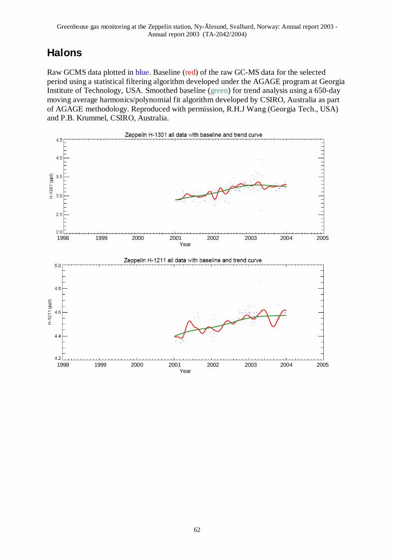
Greenhouse gas monitoring at the Zeppelin station, Ny-Ålesund, Svalbard, Norway: Annual report 2003 - Annual report 2003 (TA-2042/2004)
62
Halons Raw GCMS data plotted in blue. Baseline (red) of the raw GC-MS data for the selected period using a statistical filtering algorithm developed under the AGAGE program at Georgia Institute of Technology, USA. Smoothed baseline (green) for trend analysis using a 650-day moving average harmonics/polynomial fit algorithm developed by CSIRO, Australia as part of AGAGE methodology. Reproduced with permission, R.H.J Wang (Georgia Tech., USA) and P.B. Krummel, CSIRO, Australia.
1998 1999 2000 2001 2002 2003 2004 2005
Year
1998 1999 2000 2001 2002 2003 2004 2005
Year

Greenhouse gas monitoring at the Zeppelin station, Ny-Ålesund, Svalbard, Norway: Annual report 2003 - Annual report 2003 (TA-2042/2004)
63
Other halogenated compounds Raw GCMS data plotted in blue. Baseline (red) of the raw GC-MS data for the selected period using a statistical filtering algorithm developed under the AGAGE program at Georgia Institute of Technology, USA. Smoothed baseline (green) for trend analysis using a 650-day moving average harmonics/polynomial fit algorithm developed by CSIRO, Australia as part of AGAGE methodology. Reproduced with permission, R.H.J Wang (Georgia Tech., USA) and P.B. Krummel, CSIRO, Australia.
1998 1999 2000 2001 2002 2003 2004 2005
Year
1998 1999 2000 2001 2002 2003 2004 2005
Year
1998 1999 2000 2001 2002 2003 2004 2005
Year

Greenhouse gas monitoring at the Zeppelin station, Ny-Ålesund, Svalbard, Norway: Annual report 2003 - Annual report 2003 (TA-2042/2004)
64
1998 1999 2000 2001 2002 2003 2004 2005
Year
1998 1999 2000 2001 2002 2003 2004 2005
Year
1998 1999 2000 2001 2002 2003 2004 2005
Year

Greenhouse gas monitoring at the Zeppelin station, Ny-Ålesund, Svalbard, Norway: Annual report 2003 - Annual report 2003 (TA-2042/2004)
65
1998 1999 2000 2001 2002 2003 2004 2005
Year
Zeppelin SF6 all data
0
1
2
3
4
5
6
7
03.2000 01.2001 11.2001 09.2002 06.2003 04.2004

Norsk institutt for luftforskning (NILU) Postboks 100, N-2027 Kjeller
REPORT SERIES
SCIENTIFIC REPORT
REPORT NO. NILU OR 59/2004
ISBN 82-425-1610-3
ISSN 0807-7207
DATE SIGN. NO. OF PAGES
65
PRICE
NOK 150.-
TITLE
Greenhouse gas monitoring at the Zeppelin station, Ny-Ålesund, Svalbard, Norway
PROJECT LEADER
Ove Hermansen
Annual report 2003 NILU PROJECT NO.
O-99093
CLASSIFICATION *
A
AUTHOR(S)
N. Schmidbauer, C. Lunder, O. Hermansen, F. Stordal, J. Schaug, I.T. Pedersen, K. Holmén, O.-A. Braathen (all NILU), J. Ström (Stockholm University) CONTRACT REF.
M.V. Pettersen, SFT
REPORT PREPARED FOR Norwegian Pollution Control Authority (SFT) P.O. Box 8100 Dep. NO-0032 OSLO NORWAY
KEYWORDS
Climate
Monitoring
Zeppelin station
ABSTRACT
The report summarises the activities and results of the greenhouse gas monitoring at the Zeppelin station situated on Svalbard in arctic Norway during year 2003.
The measurement programme is performed by the Norwegian Institute for Air Research (NILU) and funded by the Norwegian Pollution Control Authority (SFT).
NORWEGIAN TITLE
Klimagassovervåking ved Zeppelinstasjonen – Årsrapport 2003
ABSTRACT (in Norwegian)
Rapporten presenterer aktiviteter og måleresultater fra klimagassovervåkingen ved Zeppelinstasjonen på Svalbard i år 2003.
Måleprogrammet utføres av Norsk institutt for luftforskning (NILU) og er finansiert av Statens forurensningstilsyn (SFT).
* Classification: A
B C
Unclassified (can be ordered from NILU) Restricted distribution Classified (not to be distributed)

Statlig program for forurensningsovervåking omfatter overvåking av forurensningsforholdene i luft og nedbør, skog, grunnvann, vassdrag, fjorder og havområder. Overvåkingsprogrammet dekker langsiktige undersøkelser av: • overgjødsling av ferskvann og kystområder • forsuring (sur nedbør) • ozon (ved bakken og i stratosfæren) • klimagasser • miljøgifter Overvåkingsprogrammet skal gi informasjon om tilstanden og utviklingen av forurensningssituasjonen, og påvise eventuell uheldig utvikling på et tidlig tidspunkt. Programmet skal dekke myndighetenes informasjonsbehov om forurensningsforholdene, registrere virkningen av iverksatte tiltak for å redusere forurensningen, og danne grunnlag for vurdering av nye tiltak. SFT er ansvarlig for gjennomføringen av overvåkingsprogrammet.
Statens forurensningstilsyn Postboks 8100 Dep, 0032 Oslo Besøksadresse: Strømsveien 96
Norsk instiutt for luftforskning Postboks 100, 2027 Kjeller Besøksadresse: Instituttveien 18
Telefon: 22 57 34 00 Telefaks: 22 67 67 06 E-post: postmottakft.no Internett: www.sft.no
Telefon: 63 89 80 00 Telefaks: 63 89 80 50 E-post: [email protected] Internett: www.nilu.no
Bestilling: http://www.sft.no/skjema.html