Gravitational Waves

Notes for Lectures at the Azores School on

Observational Cosmology

September 2011

B F Schutz

Albert Einstein Institute (AEI), Potsdam, Germanyhttp://www.aei.mpg.de, Bernard.Schutz@aei.mpg.de

References:

B F Schutz, A First Course in General Relativity (2nd ed.), Cam-

bridge University Press 2009.

B F Schutz and F Ricci, Gravitational Waves, Sources, and De-

tectors, arxiv1005.4735 (Notes of lectures given at a summer school

at Lake Como in 1999).

C W Misner, K S Thorne, and J Wheeler, Gravitation, Freeman

(1983).

Living Reviews in Relativity has an extensive section of review ar-

ticles on gravitational waves at

http://relativity.livingreviews.org

These include:

• M Pitkin, S Reid, S Rowan, and J Hough, ”Gravitational Wave

Detection by Interferometry (Ground and Space)”

• B S Sathyaprakash and B F Schutz, ”Physics, Astrophysics and

Cosmology with Gravitational Waves”

• L Blanchet, ”Gravitational Radiation from Post-Newtonian Sources

and Inspiralling Compact Binaries”

1

• P Jaranowski and A Krolak, ”Gravitational-Wave Data Analy-

sis. Formalism and Sample Applications: The Gaussian Case”

2

Contents of Lecture 1. Elementary Theory of Gravita-

tional Waves and their Detection

1. Special and general relativity. Review of Minkowski ge-

ometry; gravitation as geometry; curvature of time and space.

2. Elements of gravitational waves. Linearized waves; prop-

agation; gauge conditions; tidal gravity.

3. Measuring gravity using light propagation. Analogy

with radar; return-time monitoring along one direction; compar-

ing two directions.

4. Beam detectors Types of detectors, basic principles.

5. Energy and gravitational radiation. How energy is de-

fined; practical applications of the energy formula.

6. Interferometric gravitational wave detectors. Present

status of detector development of LIGO, VIRGO, GEO; obser-

vational results so far; expected performance of Advanced De-

tectors, including LCGT, ET.

7. Networks of detectors. Confidence; determining polariza-

tion and direction; analogy with sound detection and micro-

phones.

3

Contents of Lecture 2. Gravitational Waves from Binary

Systems: Probes of the Universe

1. Historical importance of observing orbiting systems.

Clean physics; use of astronomy of binaries to develop fundamen-

tal laws by Newton and Galileo.

2. Mass-quadrupole radiation. Radiation generation in lin-

earized theory; energy radiated in waves; radiation generation in

the full Newtonian limit.

3. Gravitational waves from a binary system. Waveform

at Newtonian order; Hulse-Taylor binary pulsar as a test of GR;

binaries as standard sirens; post-Newtonian corrections; numer-

ical studies of binaries.

4. Expected science from Advanced Detectors. Popula-

tion statistics, gamma-ray burst science, measuring local Hubble

Constant.

5. Space-based binary science. Mergers of massive black

holes; Hubble constant; discriminating among models of BH

growth in early universe; dark energy measurements.

4

Contents of Lecture 3. A Stochastic Gravitational Wave

Cosmological Background

1. Introduction. Non-thermal radiation. Weak coupling. Infor-

mation content.

2. Tensor modes from inflation. Excitation, predictions of

spectrum.

3. Post-inflation physics. Phase transitions, cosmic strings,

brane-world scenarios.

4. Astrophysical backgrounds. Binaries at different frequen-

cies.

5. Current bounds Nucleosynthesis bound; pulsar timing bounds;

LIGO’s observational upper limits.

6. Detecting backgrounds. Cross-correlation of ground-based

detectors; using a space-based instrument; pulsar timing.

5

Gravitational Waves

Notes for Lectures at the Azores School on

Observational Cosmology

September 2011

B F Schutz

Albert Einstein Institute (AEI), Potsdam, Germanyhttp://www.aei.mpg.de, Bernard.Schutz@aei.mpg.de

Lecture 1 – Elementary Theory ofGravitational Waves and their Detection

Special and General Relativity

Lectures assume familiarity with relativistic electromagnetism and

with Minkowski geometry. The metric (interval) is

ds2 = ηαβdxαdxβ,

where the symbol η denotes the matrix diag(−1, 1, 1, 1). I will take

c = 1 and use the usual summation convention on repeated indices.

Greek indices sum over all four coordinates (0..3), Latin over the

three spatial coordinates (1..3).

General relativity describes gravitation as geometry. Inspiration:

the principle of equivalence, roots back to Galileo.

• Any smooth geometry is locally flat, and in GR this means that

it is locally Minkowskian. Local means in space and time: the

local Minkowski frame is a freely-falling observer.

1

• In a general coordinate system the Minkowski equation is re-

placed by

ds2 = gαβdxαdxβ,

where g is a position-dependent symmetric 4× 4 matrix. As in

special relativity, the metric measures proper time and proper

distance. Coordinates are arbitrary in GR, but most situations

are easier to analyse in appropriately chosen coordinates. A free

particle follows a geodesic of this metric, defined as a locally

straight world-line.

• There are 4 degrees of freedom to choose coordinates, and 10

components of g: 6 “true” functions left for the geometry. The

tensorial description of the geometry is through the Riemann

curvature tensor, which contains second derivatives of g. We

will explore its meaning later.

• Derived from the Riemann tensor is the Einstein tensor G, which

is basis of the field equations

Gαβ = 8πT αβ,

where T is the stress-energy tensor, whose components contain

the energy density, momentum density, and stresses inside the

source of the field. (We also take Newton’s constant G = 1. )

In GR momentum and stress as well as energy density create

gravity.

• In non-relativistic situations, the energy density dominates, which

is the 0-0 field equation. The most important curvature for

nearly-Newtonian systems is the curvature of time, which is

measurable by the gravitational redshift of clocks. All of New-

tonian orbital motion can be derived from time-curvature: if

2

you know the gravitational redshift everywhere, you know the

Newtonian gravitational field everywhere. Relativistic particles,

such as photons, are not described by Newtonian physics; their

motion is sensitive also to the spatial curvature.

• The coordinate invariance of the theory implies that not all field

equations are independent; mathematically the Einstein tensor

is divergence-free for any metric:

∇αGαβ = 0.

This is called the Bianchi identity. It implies, from the field

equation,

∇αTαβ = 0.

This is the equation of conservation of energy and momen-

tum in the matter sources. In field theory language, coordinate

invariance is a gauge group, the conservation laws of the Bianchi

identities arise as Noether identities.

• Derivatives like ∇α are defined so that in a freely-falling frame

they are the derivatives of special relativity. Called covariant

derivatives. In a general coordinate system they involve deriva-

tives of tensor components and of basis vectors eα, so expressions

are complicated. They involve Christoffel symbols Γαβδ:

∇δeβ = Γαβδeα.

The Christoffel symbols involve the first derivatives of the metric

tensor. They vanish in a local freely falling frame, but only at

the single event where the frame is perfectly freely falling. The

second derivatives of the metric cannot in general be made to

vanish by going to any special coordinate system. You first meet

3

the Christoffel symbols (but nobody introduces you to them by

name!) in elementary vector calculus in Euclidean space, when

you compute divergences in polar coordinates and find that you

need more than just the derivatives of vector components.

• It is important to understand what the conservation law of the

stress-energy tensor means. It is conservation in a freely-falling

frame. This is the equivalence principle: in a freely falling frame,

the local matter energies are conserved. It does not represent a

conservation law with gravitational potential energy, for exam-

ple. Such global energy conservation laws are valid only if the

metric is independent of time. (We will return to this important

point below.) The local conservation law is an equation of mo-

tion. It implies, for example, that isolated small particles fall on

geodesics of the metric.

• If a tensor has zero covariant derivative in a given direction, it

is said to be parallel-transported. Thus, a vector V is parallel-

transported in the direction W if

W α∇αVβ = 0

for all β. Parallel-transport means that the field is held constant

in a freely-falling frame.

• A special case of parallel transport is the geodesic equation,

which is the statement that the four-velocity U — whose compo-

nents are Uα = dxα/dτ (where τ is proper time) — is parallel-

transported along itself:

dUα

dτ+ ΓαµνU

µU ν = 0.

4

• The second derivatives of the metric contain coordinate-invariant

information that is collected in the Riemann curvature tensor

R. An interesting definition of R involves the commutator of

covariant derivatives of a vector field V :

[∇α,∇β]V µ = RµναβV

ν.

In Minkowski spacetime, derivatives commute and the curvature

is zero. In a curved space(time), covariant derivatives in different

directions do not commute. This is most easily seen in terms

of parallel transport: vector fields that are parallel transported

tangent to a sphere along different great circles, for example, do

not coincide with one another when the great circles intersect

again.

• Another interpretation of the Riemann tensor is in terms of the

failure of parallelism in a curved space. If we start two nearby

geodesics off in the same direction, with a tangent vector U , and

if we place a connecting vector ξ between the two geodesics and

carry it along so it always links them at the same elapsed proper

time, then the connecting vector will not remain constant if the

space is not flat:

d2ξα

dτ 2= −Rα

µβνUµξβU ν.

This is called the equation of geodesic deviation.

• The mathematics of tensor calculus can get very complicated.

The expressions for the Riemann tensor in terms of the compo-

nents of the metric tensor are long and not very informative. We

will not go into such things in these lectures. They are treated

in the textbooks.

5

• Approximation methods are crucial in general relativity.

– We will deal mostly with linearized theory in these lec-

tures, where the curvature is small and spacetime is nearly

Minkowskian. Only terms of first order in the difference

between the true metric and the Minkowski metric are con-

sidered.

– Another important approximation is the post-Newtonian

approximation. GR contains Newtonian gravity as a (de-

generate) limit, where the field equations lose their time-

derivatives. One can develop an asymptotic approximation

to GR away from this limit. The limit links two parame-

ters: the gravitational field is weak and the velocities of the

sources are small. In linearized theory the field is weak but

the sources do not have to be non-relativistic.

– Perturbation theory is the study of solutions near a known

solution. This is a generalization of linearized theory. It can

study stellar stability, the orbits (with radiation reaction) of

particles near black holes, and so on.

– A final approximation method is numerical relativity: sim-

ulations of black holes and other situations are increasingly

useful in understanding GR. It can attack any problem in

principle, no matter how complicated, but of course one has

to be careful to be sure the result is a close enough approxi-

mation to the true solution.

6

Elements of gravitational waves

GR is nonlinear, fully dynamical ⇒ in general no clear distinction

between waves and the rest of the metric. The notion of a wave is

OK in certain limits:

• in linearized theory;

• as small perturbations of a smooth background metric (e.g. waves

propagating in cosmology or waves being gravitationally lensed

by the metric of a star, galaxy, or cluster);

• in post-Newtonian theory (far zone, i.e. more than one wave-

length distant from the source).

We will concentrate on linearized theory, but much of this work car-

ries over to the other cases in a straightforward way.

7

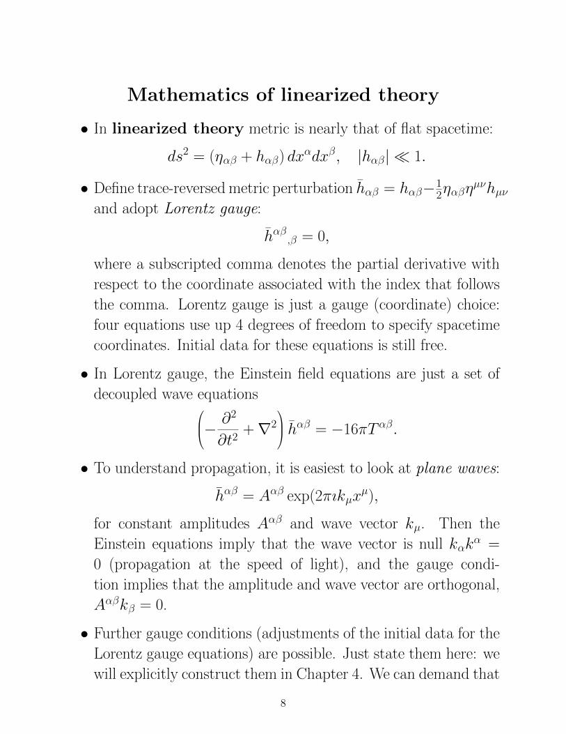
Mathematics of linearized theory

• In linearized theory metric is nearly that of flat spacetime:

ds2 = (ηαβ + hαβ) dxαdxβ, |hαβ| 1.

• Define trace-reversed metric perturbation hαβ = hαβ−12ηαβη

µνhµνand adopt Lorentz gauge:

hαβ,β = 0,

where a subscripted comma denotes the partial derivative with

respect to the coordinate associated with the index that follows

the comma. Lorentz gauge is just a gauge (coordinate) choice:

four equations use up 4 degrees of freedom to specify spacetime

coordinates. Initial data for these equations is still free.

• In Lorentz gauge, the Einstein field equations are just a set of

decoupled wave equations− ∂2

∂t2+∇2

hαβ = −16πT αβ.

• To understand propagation, it is easiest to look at plane waves:

hαβ = Aαβ exp(2πıkµxµ),

for constant amplitudes Aαβ and wave vector kµ. Then the

Einstein equations imply that the wave vector is null kαkα =

0 (propagation at the speed of light), and the gauge condi-

tion implies that the amplitude and wave vector are orthogonal,

Aαβkβ = 0.

• Further gauge conditions (adjustments of the initial data for the

Lorentz gauge equations) are possible. Just state them here: we

will explicitly construct them in Chapter 4. We can demand that

8

1. A0β = 0 ⇒ Aijkj = 0: Transverse wave; and

2. Ajj = 0: Traceless wave amplitude.

These conditions can only be applied outside a sphere surround-

ing the source. Together, they put the metric into the transverse-

traceless (TT) gauge. In TT gauge, hαβ = hαβ.

9

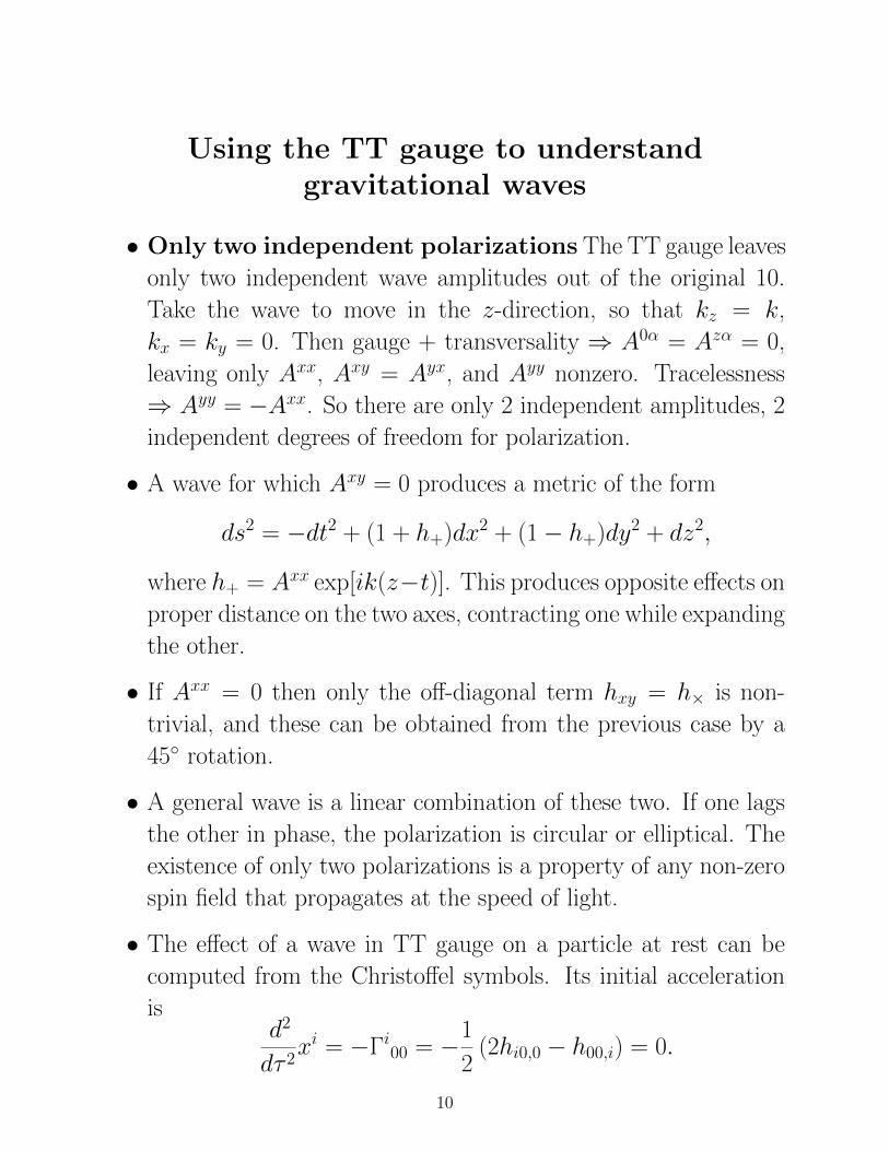
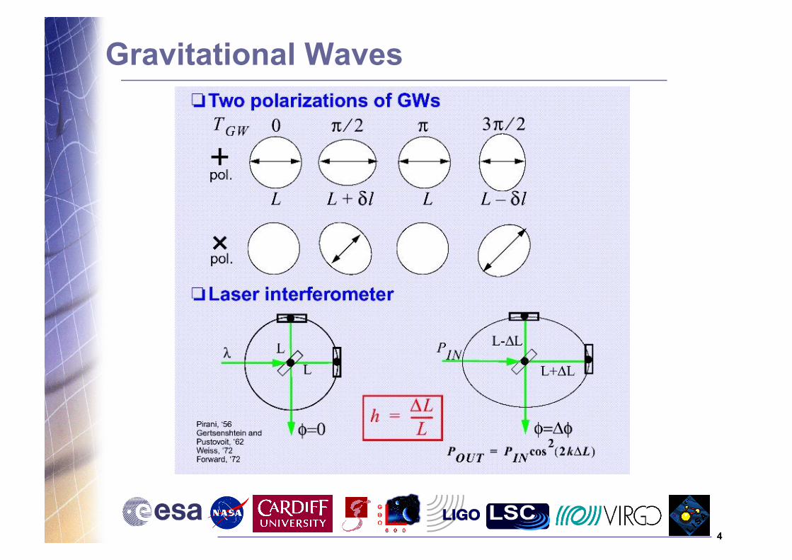
Using the TT gauge to understandgravitational waves

• Only two independent polarizations The TT gauge leaves

only two independent wave amplitudes out of the original 10.

Take the wave to move in the z-direction, so that kz = k,

kx = ky = 0. Then gauge + transversality ⇒ A0α = Azα = 0,

leaving only Axx, Axy = Ayx, and Ayy nonzero. Tracelessness

⇒ Ayy = −Axx. So there are only 2 independent amplitudes, 2

independent degrees of freedom for polarization.

• A wave for which Axy = 0 produces a metric of the form

ds2 = −dt2 + (1 + h+)dx2 + (1− h+)dy2 + dz2,

where h+ = Axx exp[ik(z−t)]. This produces opposite effects on

proper distance on the two axes, contracting one while expanding

the other.

• If Axx = 0 then only the off-diagonal term hxy = h× is non-

trivial, and these can be obtained from the previous case by a

45 rotation.

• A general wave is a linear combination of these two. If one lags

the other in phase, the polarization is circular or elliptical. The

existence of only two polarizations is a property of any non-zero

spin field that propagates at the speed of light.

• The effect of a wave in TT gauge on a particle at rest can be

computed from the Christoffel symbols. Its initial acceleration

isd2

dτ 2xi = −Γi00 = −1

2(2hi0,0 − h00,i) = 0.

10

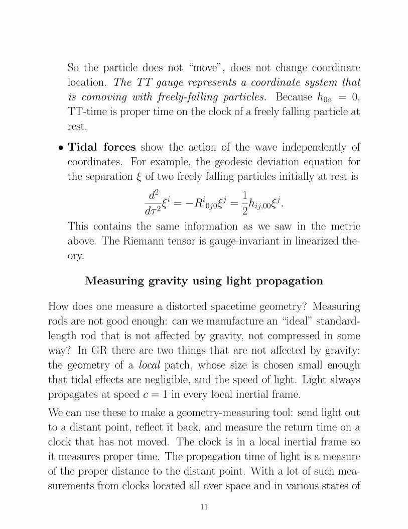
So the particle does not “move”, does not change coordinate

location. The TT gauge represents a coordinate system that

is comoving with freely-falling particles. Because h0α = 0,

TT-time is proper time on the clock of a freely falling particle at

rest.

• Tidal forces show the action of the wave independently of

coordinates. For example, the geodesic deviation equation for

the separation ξ of two freely falling particles initially at rest is

d2

dτ 2ξi = −Ri

0j0ξj =

1

2hij,00ξ

j.

This contains the same information as we saw in the metric

above. The Riemann tensor is gauge-invariant in linearized the-

ory.

Measuring gravity using light propagation

How does one measure a distorted spacetime geometry? Measuring

rods are not good enough: can we manufacture an “ideal” standard-

length rod that is not affected by gravity, not compressed in some

way? In GR there are two things that are not affected by gravity:

the geometry of a local patch, whose size is chosen small enough

that tidal effects are negligible, and the speed of light. Light always

propagates at speed c = 1 in every local inertial frame.

We can use these to make a geometry-measuring tool: send light out

to a distant point, reflect it back, and measure the return time on a

clock that has not moved. The clock is in a local inertial frame so

it measures proper time. The propagation time of light is a measure

of the proper distance to the distant point. With a lot of such mea-

surements from clocks located all over space and in various states of

11

motion, one can build up a database from which the overall geometry

can be reconstructed.

Although this sounds like a thought-experiment, we have been us-

ing light-clocks as distance measuring tools for decades. We call it

radar. Today it is even more practical to use such a technique be-

cause lasers give such precise control over the generation of the light

that ultra-precise measurements of distance are possible. Photon-

based distance measurements are the basis of all methods being used

today to directly measure time-dependent spacetime geometry, i.e.

to detect gravitational waves. Such detectors are called beam detec-

tors. To understand how beam detectors work we need to look at

the propagation of light in a gravitational wave geometry.

Let us compute the proper distance between two freely-falling bodies

(no forces on them other than gravity), which start off at rest with

respect to one another before the gravitational wave arrives. We

shall do the computation in TT gauge because in these coordinates

the bodies remain at fixed coordinate locations, which simplifies the

computation. We need to calculate the effect of the waves on the

coordinate speed of light. In the “+” metric earlier, where the wave is

traveling in the z-direction, a null geodesic moving in the x-direction

has effective speed dxdt

2 =1

1 + h+.

This is a coordinate speed, no contradiction to special relativity.

12

• Suppose light is directed along the x-direction and the gravita-

tional wave is moving in the z-direction with a +-polarization

of any waveform h+(t) along this axis. (It is a plane wave, so

its waveform does not depend on x.) Then a photon emitted

at time t from the origin reaches the distant object, which at a

fixed coordinate position x = L, at the coordinate time

tfar = t +∫ L0

[1 + h+(t(x))]1/2 dx,

where the argument t(x) denotes the fact that one must know the

time to reach position x in order to calculate the wave field. This

implicit equation can be solved in linearized theory by using the

fact that h+ is small. Then we can set t(x) = t+ x and expand

the square root. The result is

tfar = t + L +1

2

∫ L0h+(t + x)dx.

In our distance meter, the light is reflected back, so the whole

trip takes

treturn = t + 2L +1

2

[∫ L0h+(t + x)dx +

∫ L0h+(t + L + x)dx

].

• In practice, to see if a gravitational wave has arrived, one moni-

tors changes in the time for the return trip as a function of time

at the origin. The rate of change of the return time as a function

of the start time t:

dtreturndt

= 1 +1

2[h+(t + 2L)− h+(t)] .

This depends only on the wave amplitude when the beam leaves

and when it returns. Interestingly, for this special geometry, it

does not involve the wave amplitude at the other end.

13

• The wave amplitude at the other end does get involved if the

wave travels at an angle θ to the z-axis in the x − z plane.

If we re-do this calculation, allowing the phase of the wave to

depend on x in the appropriate way, and taking into account the

fact that hxx is reduced if the wave is not moving in a direction

perpendicular to x, we can find

dtreturndt

= 1 +1

2(1− sin θ)h+(t + 2L)− (1 + sin θ)h+(t)

+2 sin θh+[t + L(1− sin θ)] .

This three-term relation is the starting point for analyzing the

response of all beam detectors.

14

Beam detectors

If a detector is small compared to the wavelength λ of a gravitational

wave, then once can do a Taylor expansion on L. For the simple case

of light moving along the x-axis, we get from above

dtreturndt

= 1 + h+(t)L + O(L2).

(Since h+ ∼ 2πh+/λ, this really is a Taylor expansion in the small

dimensionless parameter L/λ.) If we take another time-derivative to

getd2treturndt2

= h+(t)L + O(L2),

we can link this with the equation of geodesic deviation that we wrote

down earlier:d2

dτ 2ξi =

1

2hij,00ξ

j.

From this point of view, the central body can consistently assume

that the distant body is subject to a simple force, proportional to the

second time-derivative of the metric. We call this the tidal force, and

it is a consistent approximation provided the experimental region is

small. This is true for laser interferometric detectors on the Earth,

and indeed for the question of how tides are raised on the Earth by

the Moon and Sun. But a gravitational wave detector in space would

be too large for this approximation to hold, and for pulsar timing the

approximation makes no sense at all.

The experiment as described assumes that we can measure time accu-

rately enough on the central clock to detect the gravitational wave.

Unfortunately, wave amplitudes are so small that the time varia-

tions are below the accuracies of our best clocks. The only way

15

to make such measurements is to compare two different directions.

An interferometer can be thought of as a light-time-return compari-

son machine, sending photons off in two perpendicular directions and

sensing variations in their relative return times by watching for shifts

in their interference patterns when they return. Since the action of a

gravitational wave is anisotropic (different in x, y, and z directions),

this comparison can detect the wave in almost all cases.

There are several kinds of beam detectors:

• Ranging to spacecraft. Both NASA and ESA perform ex-

periments in which they monitor the return time of communica-

tion signals with interplanetary spacecraft for the characteristic

effect of gravitational waves. For missions to Jupiter and Saturn,

for example, the return times are of order 2 − 4 × 103 s. Any

gravitational wave event shorter than this will appear 3 times

in the time-delay: once when the wave passes the Earth-based

transmitter, once when it passes the spacecraft, and once when

it passes the Earth-based receiver. Searches use a form of data

analysis using pattern matching. Using two transmission fre-

quencies and very stable atomic clocks, it is possible to achieve

sensitivities for h of order 10−13, and even 10−15 may soon be

reached. This technique really does use only one arm and a

clock, so it is limited by clock accuracies.

16

• Pulsar timing. Many pulsars, particularly the old millisecond

pulsars, are extraordinarily regular clocks, with random timing

irregularities too small for the best atomic clocks to measure. If

one assumes that they emit pulses perfectly regularly, then one

can use observations of timing irregularities of single pulsars to

set upper limits on the background gravitational wave field. Here

the 3-term formula is replaced by a simpler two-term expression,

because we only have a one-way transmission. Moreover, the

transit time of a signal to the Earth from the pulsar may be

thousands of years, so we cannot look for correlations between

the two terms in a given signal. Instead, the delay is a combi-

nation of the effects of waves at the pulsar when the signal was

emitted and waves at the Earth when it is received.

If one simultaneously observes two or more pulsars, the Earth-

based part of the delay is correlated, and this offers a means of

actually detecting long-period gravitational waves. Observations

require timescales of several years in order to achieve the long-

period stability of pulse arrival times, so this method is suited

to looking for strong gravitational waves with periods of sev-

eral years. Observations are currently underway at a number

of observatories. These include Parkes Pulsar Timing Array, the

European Pulsar Timing Array, and the American Nanograv col-

laboration. Detections of random backgrounds of gravitational

waves from the mergers of supermassive black holes may well

take place before 2020. Longer-range plans include SKA (the

Square Kilometer Array) and its pathfinders.

• Interferometry. As mentioned above, an interferometer es-

sentially measures the difference in the return times along two

different arms. The response of each arm will follow the three-

17

term formula, but with different values of θ, depending in a

complicated way on the orientation of the arms relative to the

direction of travel and polarization of the wave. Ground-based

interferometers are small enough to use the small-L formulas we

derived above. These include the two LIGO sites in the USA

(Hanford, Washington, and Livingston, Louisiana), the VIRGO

detector near Pisa, Italy, the GEO600 detector near Hannover,

Germany, and the LCGT detector under construction in Japan

in the Kamiokande underground facility.

But LISA, the proposed space-based interferometer, would be

larger than a wavelength of gravitational waves for frequencies

above 10 mHz, so a detailed analysis based on the 3-term formula

is needed.

18

Energy and Gravitational Radiation

• How waves carry energy. Energy has been one of the most

confusing aspects of gravitational wave theory and hence of gen-

eral relativity. It caused much controversy, and even Einstein

himself took different sides of the controversy at different times

in his life. Physicists today have reached a wide consensus. The

problem is difficult because of the equivalence principle: in a

local frame there are no waves and hence no local definition of

energy that can be coordinate-invariant. Moreover, a wave is a

time-dependent metric, and in such spacetimes there is no global

energy conservation law. (Recall that conservation laws are asso-

ciated with symmetry. Angular momentum is conserved only in

axisymmetric systems, or in systems governed by axisymmetric

forces or fields. Likewise, energy is conserved on in time-invariant

systems.) Energy is only well-defined in certain regimes, which

coincide with those for which waves can be cleanly separated

from ”background” metrics.

• Asymptotically flat spacetimes. Relativists have intro-

duced the concept of asymptotic flatness, which idealises an

isolated body, one whose geometry becomes flat far away. If the

body is stationary (time-independent) then test fields (falling

particles) will have conserved energy. If there is a small pertur-

bation that can be treated as a wave, then its energy will be

conserved, in the sense that the total mass-energy of the sys-

tem (as measured by planetary orbits far away) decreases as the

waves leave.

• Wave flux. The energy carried by a wave as it leaves a body

19

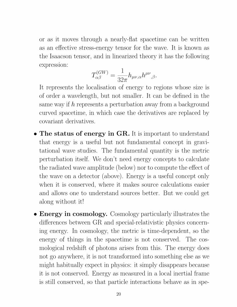
or as it moves through a nearly-flat spacetime can be written

as an effective stress-energy tensor for the wave. It is known as

the Isaacson tensor, and in linearized theory it has the following

expression:

T(GW )αβ =

1

32πhµν,αh

µν,β.

It represents the localisation of energy to regions whose size is

of order a wavelength, but not smaller. It can be defined in the

same way if h represents a perturbation away from a background

curved spacetime, in which case the derivatives are replaced by

covariant derivatives.

• The status of energy in GR. It is important to understand

that energy is a useful but not fundamental concept in gravi-

tational wave studies. The fundamental quantity is the metric

perturbation itself. We don’t need energy concepts to calculate

the radiated wave amplitude (below) nor to compute the effect of

the wave on a detector (above). Energy is a useful concept only

when it is conserved, where it makes source calculations easier

and allows one to understand sources better. But we could get

along without it!

• Energy in cosmology. Cosmology particularly illustrates the

differences between GR and special-relativistic physics concern-

ing energy. In cosmology, the metric is time-dependent, so the

energy of things in the spacetime is not conserved. The cos-

mological redshift of photons arises from this. The energy does

not go anywhere, it is not transformed into something else as we

might habitually expect in physics: it simply disappears because

it is not conserved. Energy as measured in a local inertial frame

is still conserved, so that particle interactions behave as in spe-

20

cial relativity. But when a particle is followed over a long time,

so that the local inertial frame is not a good approximation, then

the energy changes.

• Gravitational waves in cosmology. As remarked before, it

is not possible to talk sensibly about gravitational waves unless

the wavelength is small compared to the curvature scale. In

cosmology that is the “radius” of the universe, or the Hubble

scale/horizon size. So any perturbations smaller than the horizon

size will propagate as gravitational waves following the same

laws of geometrical optics that photons follow. In particular

the energy of the waves gets redshifted in the same way as for

photons.

21

Practical applications of the energy formula

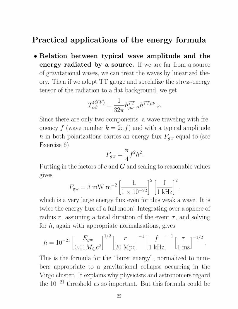
• Relation between typical wave amplitude and the

energy radiated by a source. If we are far from a source

of gravitational waves, we can treat the waves by linearized the-

ory. Then if we adopt TT gauge and specialize the stress-energy

tensor of the radiation to a flat background, we get

T(GW )αβ =

1

32πhTTµν ,αh

TTµν,β.

Since there are only two components, a wave traveling with fre-

quency f (wave number k = 2πf ) and with a typical amplitude

h in both polarizations carries an energy flux Fgw equal to (see

Exercise 6)

Fgw =π

4f 2h2.

Putting in the factors of c and G and scaling to reasonable values

gives

Fgw = 3 mW m−2 h

1× 10−22

2 f

1 kHz

2 ,which is a very large energy flux even for this weak a wave. It is

twice the energy flux of a full moon! Integrating over a sphere of

radius r, assuming a total duration of the event τ , and solving

for h, again with appropriate normalisations, gives

h = 10−21 Egw

0.01Mc2

1/2 r

20 Mpc

−1 f

1 kHz

−1 [ τ

1 ms

]−1/2.

This is the formula for the “burst energy”, normalized to num-

bers appropriate to a gravitational collapse occurring in the

Virgo cluster. It explains why physicists and astronomers regard

the 10−21 threshold as so important. But this formula could be

22

applied to binary systems radiating away their orbital gravita-

tional binding energy over long periods of time τ , for example.

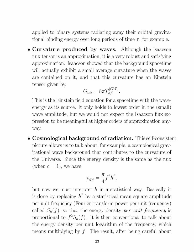
• Curvature produced by waves. Although the Isaacson

flux tensor is an approximation, it is a very robust and satisfying

approximation. Isaacson showed that the background spacetime

will actually exhibit a small average curvature when the waves

are contained on it, and that this curvature has an Einstein

tensor given by.

Gαβ = 8πT(GW )αβ .

This is the Einstein field equation for a spacetime with the wave-

energy as its source. It only holds to lowest order in the (small)

wave amplitude, but we would not expect the Isaacson flux ex-

pression to be meaningful at higher orders of approximation any-

way.

• Cosmological background of radiation. This self-consistent

picture allows us to talk about, for example, a cosmological grav-

itational wave background that contributes to the curvature of

the Universe. Since the energy density is the same as the flux

(when c = 1), we have

ρgw =π

4f 2h2,

but now we must interpret h in a statistical way. Basically it

is done by replacing h2 by a statistical mean square amplitude

per unit frequency (Fourier transform power per unit frequency)

called Sh(f ), so that the energy density per unit frequency is

proportional to f 2Sh(f ). It is then conventional to talk about

the energy density per unit logarithm of the frequency, which

means multiplying by f . The result, after being careful about

23

averaging over all directions of the waves and all independent

polarization components, is

dρgwd ln f

= 4π2f 3Sh(f ).

Finally, what is of most interest is the energy density as a frac-

tion of the closure or critical cosmological density, given by the

Hubble constant H0 as ρc = 3H20/8π. The resulting ratio is

called Ωgw(f ):

Ωgw(f ) =32π3

3H20

f 3Sh(f ).

24

Status of Interferometric detectors

The interferometric gravitational wave detectors operating today are

the most sensitive measuring instruments ever built. Capable of

measuring small changes in the proper separation of their mirrors of

order 10−16 cm, which is significantly smaller than the diameter of a

proton. It has taken decades of development to reach this sensitivity

and to be able to control the instruments well enough that they

remain on-line for most of the time during an observing run (over

90% of the time in the case of GEO600). The observing frequency

band of these detectors is from about 40 Hz up to a few kHz.

Yet even with this sensitivity the detectors would have to be very

lucky, on our present understanding of potential sources, to have

detected anything yet. LIGO, GEO600, and VIRGO have done two

observing runs, called S5 (2005-7) and S6 (2009-10) with a small

sensitivity upgrade in between, and from these runs have come a large

number of papers setting upper limits on possible sources, including

on the stochastic background from the Big Bang. We will consider

that limit in the third lecture. Other limits have constrained the

smoothness of some neutron stars (some are smoother than parts in

107, much smoother than the Earth) and the fraction of the energy-

loss of the Crab pulsar that is going into gravitational waves (less

than 1%). But a further upgrade is needed to make direct detections

happen within a reasonable amount of time.

LIGO at present is upgrading to what is called Advanced LIGO,

which will be 10 times more sensitive than in S5 when it begins

operating again, probably around 2015. VIRGO is currently in an

observing run (S6e) with GEO600 but will soon begin a similar up-

grade. GEO600 is upgrading in a different manner, aimed at higher

25

frequencies (several kHz), but is also mainly providing cover (”as-

trowatch”) while the bigger detectors are upgrading. Regular de-

tections are confidently expected starting in the time-frame 2015-16

because a factor of 10 increase in sensitivity translates in to a factor

10 improvement in the detection range, which increases the detection

volume by 1000. Even pessimistic source rate estimates suggest a few

events per year in such a volume, and optimistic scenarios suggest

hundreds of events per year.

Recently the Japanese have approved and funded the Large Cryo-

genic Gravitational-wave Telescope (LCGT), which will hopefully be

able to operate soon after 2016 (depending on the speed with which

funds can be released). It will compete in sensitivity with Advanced

LIGO, but will at the same time introduce two new technologies that

are needed for further improvements in sensitivity: cryogenic cooling

of the mirrors and going underground.

The Europeans have looked ahead and, after a multi-year study

funded by the EU, have proposed a design for a so-called third-

generation detector called the Einstein Telescope (ET). This would

advance the sensitivity a further factor of 10 beyond Advanced LIGO

and push the lower frequency limit down to a few Hz. This upgrade

cannot be done in the existing instruments, and would require a

new instrument, cryogenically cooled, 10 km long, and a few hun-

dred metres beneath the ground. The sensitivity, however, would be

enough to survey the entire universe for binary mergers of neutron

stars and/or black holes, a source that we will treat in more detail

in the second lecture.

Pulsar timing arrays were started about 5 years ago but are now

being very actively built up, and observatories are giving them more

26

and more time. Because pulsars are good clocks only when averaged

over a long time, these arrays are sensitivity to gravitational waves

of periods of a year or more. They are expecting that the largest

signal will be a random background from countless orbiting systems

of supermassive black holes, and we will return to this in the third

lecture.

The frequency band around 1 mHz is very rich in interesting sources,

including binaries in our Galaxy and binaries of massive black holes

in external galaxies. To observe in this band requires going into

space, and ESA adopted the proposed LISA mission as long ago as

1995. The new technology required for LISA will be launched in

LISA Pathfinder sometime in 2013-14. The recent funding problems

in NASA have caused it to withdraw from its partnership in LISA,

so ESA is again considering whether it can proceed with a somewhat

de-scoped mission by itself.

27

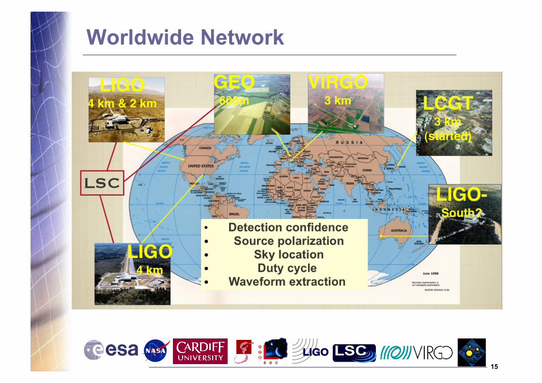
Detector Networks

The current suite of ground-based interferometers all work closely

together. LIGO and GEO are part of the same collaboration, the

LIGO Scientific Collaboration (LSC), where technologies pioneered

in GEO600 are transferred to LIGO for its upgrade, and where scien-

tists work in teams on the experiment and data analysis. Data from

the LSC detectors is exchanged with data from VIRGO, and jointly

analysed. When LCGT comes online it is expected that this model

will continue to hold.

This cooperation is driven by the needs of the science. No single

detector could have enough confidence to claim a detection of such

a weak signal by itself: one must see the signal in more than one

detector for confidence. But also recall that interferometers are not

highly directional; they are not pointed telescopes. So to get direc-

tional information one uses time-delays among the arrival time of

the signals at different detectors. Having multiple detectors also is

needed in order to measure both polarizations of the gravitational

wave. In these respects, detectors behave in the same way as sound

microphones: one needs stereo (or better) for directionality. Key

scientific results, like measuring the distance to binary systems (see

the next lecture), depend on having the information a network can

measure: polarization and sky location.

LIGO is currently exploring the possibility of moving one of the two

large Advanced detectors it has been planning for its Hanford loca-

tion, and putting it in Australia. This would greatly improve the

information available from multiple locations, especially the localiza-

tion of directions. it would also improve the ability of the network

to distinguish real signals from random background noise events. If

28

it is not possible to find the funding in Australia, another potential

good location for the detector would be India.

LISA’s design, with three spacecraft and three active arms measuring

the changes in the separations, allows the signals to be combined into

three different gravitational wave measurements, essentially treating

each spacecraft as the central station of an interferometer based on

the two arms that converge there. With these signals, LISA measures

the polarization of an incoming wave automatically, and the configu-

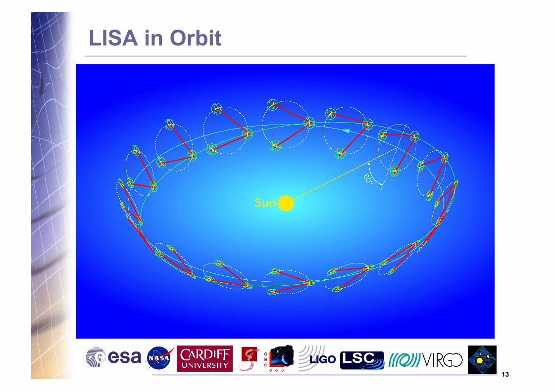
ration also gives some directional capabilities. But LISA’s direction

finding comes mainly from its orbital motion around the Sun and

the Doppler shift in the signals that this produces. For a short-lived

signal this does not help, but for a signal that lasts a good fraction of

a year, which is the case for most of LISA’s sources, then the Doppler

effect is measurable and points to the location of the source on the

sky.

29

LISA 1

Azores School on Cosmology

Gravitational Waves

1-5 September 2011 B F Schutz

Albert Einstein Institute (AEI), Potsdam, Germany and

School of Physics and Astronomy, Cardiff University

2

Download Lecture Notes

  You can find the lecture notes available for download at

http://www.aei.mpg.de/~schutz/download/lectures/AzoresCosmology

  There are 4 files: an outline, and the three lectures.

3

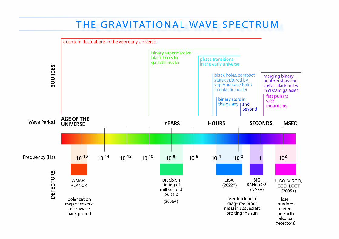
LIGO, VIRGO, GEO, LCGT

(2005+)

LISA (2022?)

(2005+)

WMAP, PLANCK

4

Gravitational Waves

5

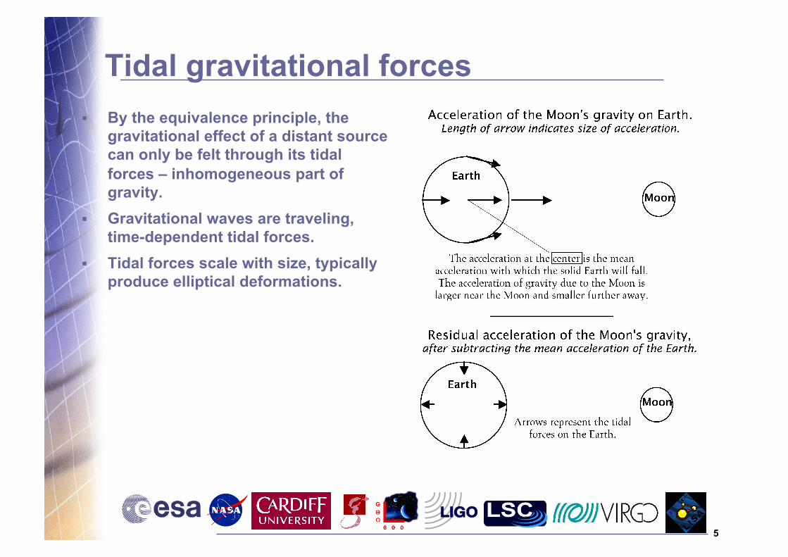
Tidal gravitational forces   By the equivalence principle, the

gravitational effect of a distant source can only be felt through its tidal forces – inhomogeneous part of gravity.

  Gravitational waves are traveling, time-dependent tidal forces.

  Tidal forces scale with size, typically produce elliptical deformations.

6

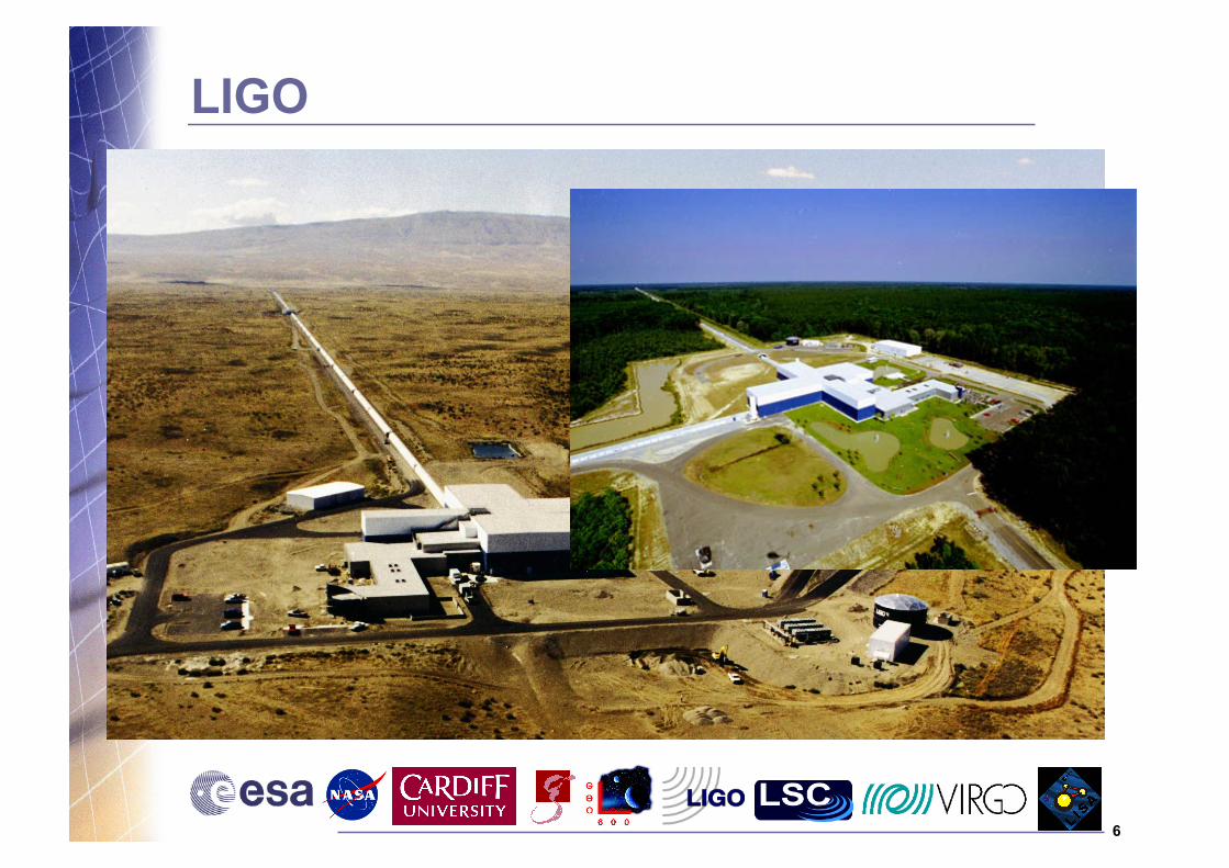
LIGO

  Locations: Hanford WA, Livingston, LA

  Partners: Caltech, MIT (NSF facility)

  Length: 4km, 2km at Hanford; 4 km at Livingston

  Target sensitivity 10-21 at 200 Hz reached in 2005

7

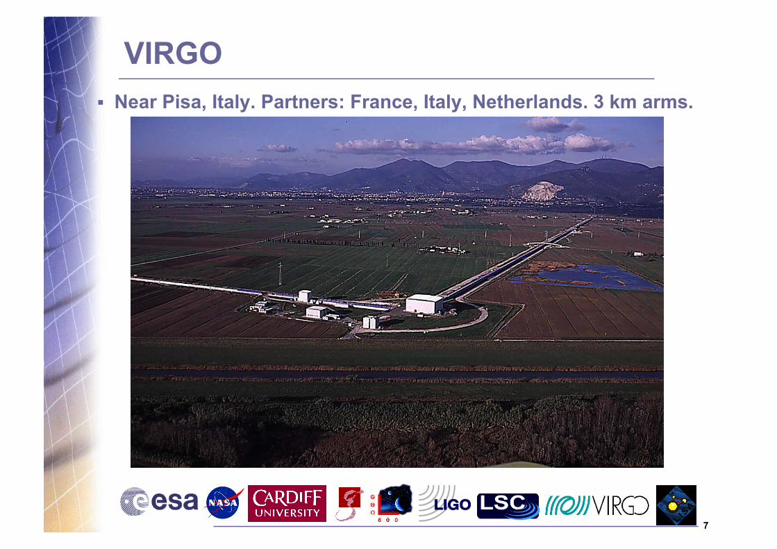
VIRGO   Near Pisa, Italy. Partners: France, Italy, Netherlands. 3 km arms.

8

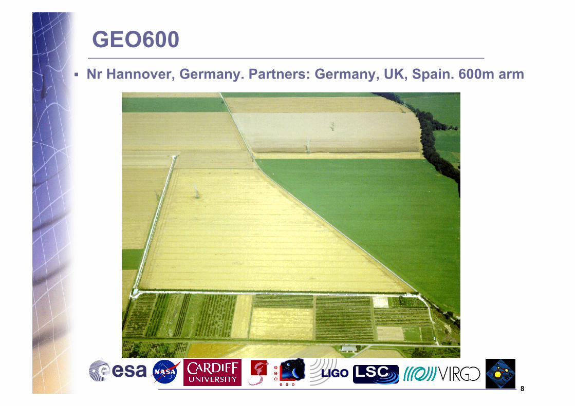
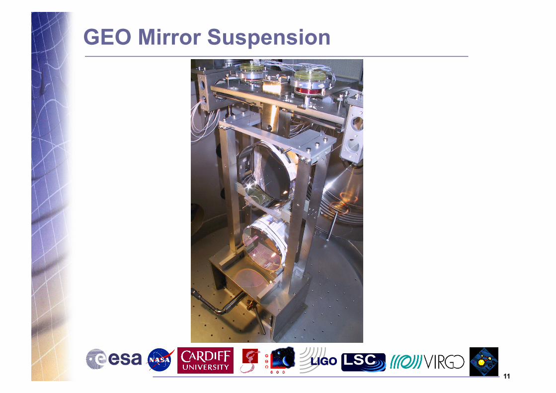
GEO600   Nr Hannover, Germany. Partners: Germany, UK, Spain. 600m arm

9

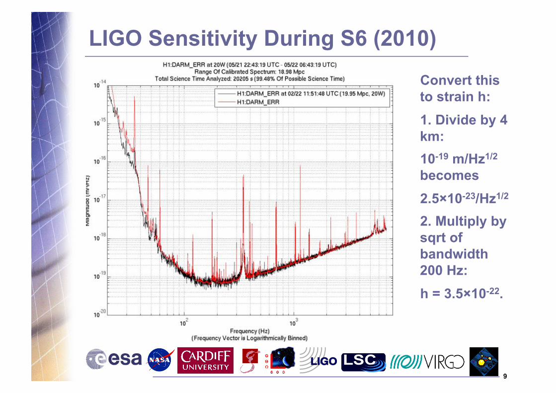
LIGO Sensitivity During S6 (2010)

  Convert this to strain h:

  1. Divide by 4 km:

  10-19 m/Hz1/2 becomes

  2.5×10-23/Hz1/2

  2. Multiply by sqrt of bandwidth 200 Hz:

  h = 3.5×10-22.

10

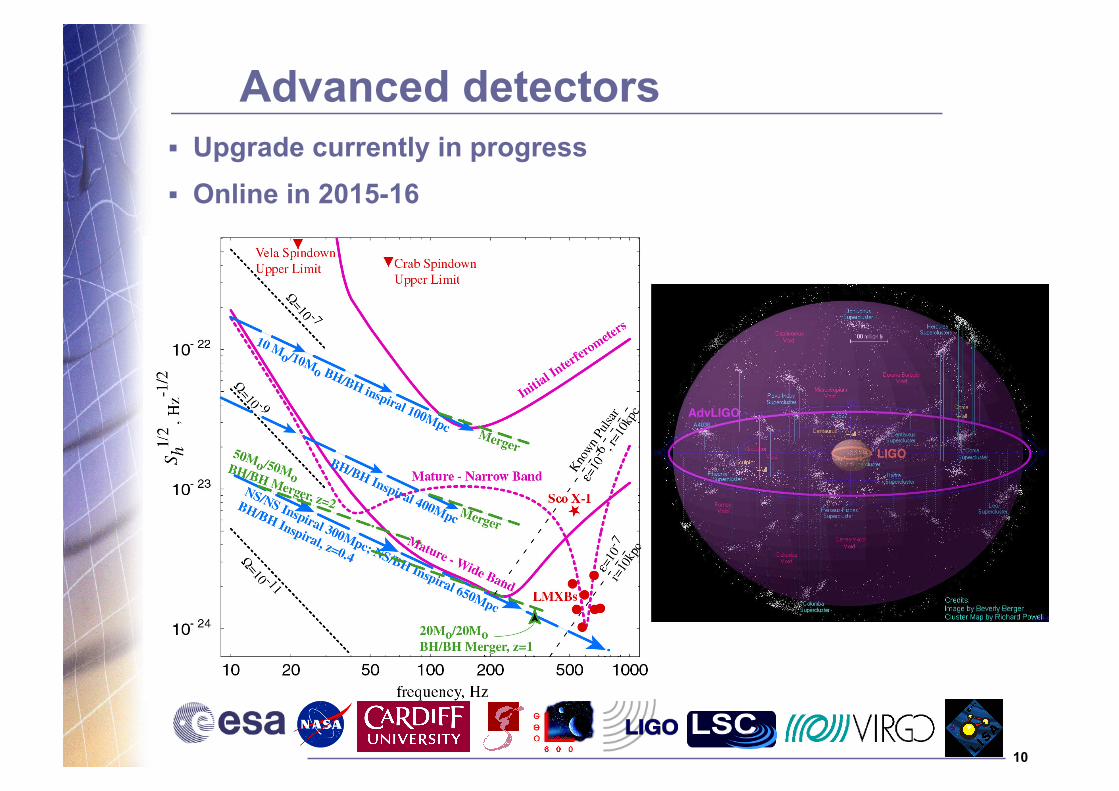
Advanced detectors   Upgrade currently in progress   Online in 2015-16

11

GEO Mirror Suspension

12

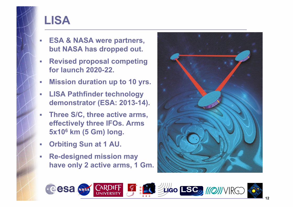
LISA   ESA & NASA were partners,

but NASA has dropped out.   Revised proposal competing

for launch 2020-22.   Mission duration up to 10 yrs.   LISA Pathfinder technology

demonstrator (ESA: 2013-14).   Three S/C, three active arms,

effectively three IFOs. Arms 5x106 km (5 Gm) long.

  Orbiting Sun at 1 AU.   Re-designed mission may

have only 2 active arms, 1 Gm.

13

LISA in Orbit

14

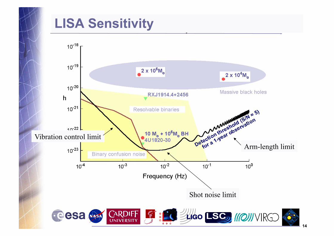
Vibration control limit

Shot noise limit

Arm-length limit

LISA Sensitivity

15

Worldwide Network