The Journal of Cosmology

Journal of Cosmology, 2011, Vol 13, In Press. JournalofCosmology.com, 2011

Observational Evidence Favors a Static Universe

Part 1

David F. CrawfordSydney Institute for Astronomy,

School of Physics, University of Sydney.NSW, Australia

ABSTRACT

The common attribute of all Big Bang cosmologies is that they are based on the assumption that the universe is expanding. However examination of the evidence for this expansion clearly favors a static universe. This is the first part (of a three part report) which investigates the topics: Tolman surface brightness, angular size, type 1a supernovae, gamma ray bursts, galaxy distributions, quasar distributions, radio source distributions, quasar variability in time and the Butcher–Oemler effect. An analysis of the best raw data for these topics shows that they are consistent with expansion only if there is evolution such that the effects of expansion are cancelled. Whereas the conclusions in Part 1 would be valid for any reasonable static cosmology the analysis of the topics in Part 2 require specific characteristics of curvature cosmology, which is a tiredlight cosmology that predicts a well defined static and stable universe. A complete description of curvature cosmology is provided in Part 3.

Keywords: Big Bang, Infinite Universe, Steady State Universe, Static Universe, Expanding Universe

Observational evidence favors a static universe

Part 1

1 Introduction

The common attribute of all Big Bang cosmologies (BB) is that they are based

on the assumption that the universe is expanding (Peebles, 1993). An early al-

ternative was the steady-state theory of Hoyle, Bondi and Gold (described with

later extensions by Hoyle et al. (2000)) that required continuous creation of

matter. However steady-state theories have serious difficulties in explaining the

cosmic microwave background radiation. This left BB as the dominant cosmol-

ogy but still subject to criticism. Recently Lal (2010) and Joseph (2010) have

continued major earlier criticisms of Big Bang cosmologies (Ellis, 1984; Lerner,

1991; Disney, 2000; Van Flandern, 2002). Whereas most of theses criticisms

have been of a theoretical nature this paper concentrates on whether observa-

tional data supports BB or a static cosmological model, curvature cosmology

(CC), described below.

Expansion produces two distinct effects. The first effect of expansion is the

increasing redshift with distance as described by Hubble’s law. This could be

due to either a genuine expansion or resulting from a tired-light phenomenon.

The second effect of expansion is time dilation resulting from the slowing down

of the arrival times of the photons as the source gets further away. Part 1 con-

centrates on the evidence for expansion as shown by time dilation and shows

that the evidence, with the exception of type 1a supernovae, is only consis-

tent with BB if there is evolution in both luminosity and in angular size that

3

closely cancels the effects of time dilation. To illustrate that a static cosmology

can explain the data, a particular model, curvature cosmology (CC), is used.

Curvature cosmology is based on the hypothesis of curvature redshift and the

hypothesis of curvature pressure. Curvature redshift arises from the principle

that any localized wave travelling in curved space time will follow geodesics and

be subject to geodesics focussing. Since this will alter the transverse properties

of the wave some of its properties such as angular momentum will be altered

which is contrary to quantum mechanics. For a photon the result is an interac-

tion that results in three new photons. One with almost identical energy and

momentum as the original and two extremely low energy secondary photons. In

effect the photon loses energy via an interaction with curved space-time. The

concept of curvature pressure arises from the idea that the density of particles

produce curved space-time. Then as a function of their velocity there will be a

reaction pressure that acts to decrease the local space-time curvature.

Part 2 extends the comparison of BB with CC and shows that many obser-

vations such as the background X-ray radiation and the cosmic microwave back-

ground radiation are consistent with CC. The main difference between Part 1

and Part 2 is that Part 1 uses the properties of CC that would be applicable

to most reasonable static cosmologies whereas Part 2 uses specific properties of

CC. Part 3 has the full description of curvature cosmology and several other

cosmological topics. In addition it shows that curvature pressure could explain

the solar neutrino deficiency and it is shown the Pioneer 10 anomalous accel-

eration can be explained by the effects of curvature redshift that is produced

by interplanetary dust provided the density of the dust is a little higher than

current estimates.

4

Since the major difference between BB and static cosmologies comes from

from the time dilation terms in BB, minor differences between different ex-

pansion cosmologies are not particularly important here; it is the broad brush

approach that is relevant. Nevertheless to provide appropriate numerical quan-

tities the evaluation is based on a particular BB cosmology, the (ΛCDM) model,

which is defined in Section 2.1 by the equations for angular size, volume and

distance modulus. A problem in evaluating a well established cosmology like

Big Bang cosmology is that all of the observations have been analyzed within

the BB paradigm. Thus there can be subtle effects that may lead to a possible

bias. In order to avoid this bias and wherever possible comparisons are made

using original observations.

Section 3 discusses the theoretical justification for the basic and additional

hypotheses that have been incorporated into the cosmologies. For BB these

includes inflation, dark matter and dark energy. For CC the hypotheses are

curvature redshift and curvature pressure.

The test for Tolman surface brightness in Section 4 is through the expected

variation of apparent surface brightness with redshift. The results strongly favor

a static universe but could be consistent with BB provided there is luminosity

evolution.

The relationship between angular size and linear size in BB includes a aber-

ration factor, due to time dilation, of (1 + z) that does not occur in static

cosmologies. However the available data does not support the inclusion of this

factor and is more consistent with a static universe.

Next it is argued that the apparent time dilation of the supernova light

curves is not due to expansion. The analysis is complex and is based on the

5

premise that the most constant characteristic of the supernova explosion is its

total energy and not its peak magnitude. If this is correct, then selection effects

can account for the apparent time dilation. The CC analysis is in complete

agreement with the known correlation between peak luminosity and light curve

duration. Furthermore the analysis overcomes a serious problem with the cur-

rent redshift distribution of supernovae. Finally using CC the distribution of

the total energy for each supernova as a function of (1 + z) has an exponent of

0.047 ± 0.089. This shows that there is no redshift dependence that occurs in

the BB analysis. Thus there is no need for dark energy.

The raw data of various time measures taken from the light curves for gamma

ray bursts (GRB) show no evidence of the time dilation that is expected in

BB. Since it can be argued that evolutionary and other effects that may have

cancelled the expected time dilation in BB are unlikely: a reasonable conclusion

is that there is no time dilation in GRB.

It is shown for galaxies with types E–Sa that have a well a defined peak

in their luminosity distribution the magnitude of this peak is independent of

redshift when the analysis was done using a static cosmology.

Analysis of quasar distributions in BB shows that luminosity evolution is

required to explain the observations. A novel method is used to analyst the

quasar distribution. Because the quasar distribution is close to an exponential

distribution in absolute magnitude (power law in luminosity) then for a small

redshift range it is also an exponential distribution in apparent magnitude.

Then for a small redshift range it is possible to use statistical averages to get an

estimate of the distance modulus directly from the raw data. The only input

required from the cosmological model is the variation of volume with redshift.

6

The results are shown in Fig. 4. They show much better agreement with CC

than with BB.

An analysis of the distribution of radio sources is included in this section not

because of explicit evidence of time dilation but because it has been generally

accepted that the distribution can only be explained by having strong evolution.

It is shown that a distribution of radio sources in a static universe can have a

good fit to the observations.

Hawkins (2010, 2001, 2003) has been monitoring quasar variability using a

Fourier method since about 1975 and finds no variation in their time scales with

redshift. Although it is generally accepted that the variations are intrinsic to

the quasar there is a possibility that they may be due to micro-lensing which

could place their origin to modulation effects in our own galaxy.

The Butcher–Oemler effect of the increasing proportion of blue galaxies in

clusters at higher redshift is shown to be non-existent or at least greatly exag-

gerated.

Except for a few cross-references the sub-sections on observational topics

are self contained and can be read independently. Since many of the topics

use statistical estimation methods and in particular linear regression. A brief

summary of the general linear regression and the treatment of uncertainties is

provided in the appendix.

2 Cosmographic Parameters

Just like the Doppler shift the cosmological redshift z is independent of the

wavelength of the spectral line. In terms of wavelength, the redshift z is z =

7

(λ0/λ−1) where λ0 is the observed wavelength and λ is the emitted wavelength.

In terms of frequency, ν, and photon energy, E, the redshift is z = ν/ν0 − 1 =

E/E0 − 1. The basic cosmological equations needed to analyst observations

provide the conversion from apparent magnitude to absolute magnitude, the

relationship between actual lateral measurement and angle and the volume as

a function of redshift.

The conversion from apparent magnitude, m, to absolute magnitude, M , is

given by the equation

M = m − µ(h) − Kz(λ0), (1)

where µ(h) is the distance modulus that strongly depends on the assumed cos-

mology and Kz(λ0) is the K-correction that allows for the difference in the

spectrum between the emitted wavelength and the observed wavelength (Rowan-

Robertson, 1985; Hogg et al., 2002) and is independent of the assumed cosmol-

ogy. For a small bandwidths and luminosity L(λ) it is

Kz(λ0) = −2.5 log(

L(λ)(1 + z)L(λ0)

). (2)

Note that the bandwidth ratio is included in the definition of the K-correction.

The Hubble constant H0 is the constant of proportionality between the appar-

ent recession speed v and distance d. That is v = Hd. It is usually written

H0 = 100h km s−1 Mpc−1 where h is a dimensionless number. Unless otherwise

specified it is assumed to have the value h = 0.7.

2.1 Big Bang cosmology (BB)

The fundamental premise of Big Bang cosmology is that the universe is expand-

ing with a scale factor proportional to (1 + z). A more detailed account can

8

be found in Peebles (1993); Peacock (1999). The analysis is simplified by using

comoving coordinates that describe the non-Euclidean geometry without expan-

sion. Note that in BB the Hubble constant is a function of redshift hence the

use of a zero subscript to denote the current value. A problem with BB is that

it is only the distances between large objects that are subject to the expansion.

It is generally accepted that any objects smaller than clusters of galaxies which

are gravitationally bound do not follow the Hubble flow.

The current version of Big-Bang cosmology is the cold dark matter (ΛCDM)

or concordance cosmology that has a complex expression for its parameters that

depends on the cosmological energy density ΩΛ. Regardless of the name, the

BB model used here is defined by the following equations. Following Goobar &

Perlmutter (1995) (with corrections from Perlmutter et al. (1997); Hogg (1999)),

the function f(x) is defined by

f(z) =∫ z

0

dz

(√

((1 + z)3 − 1)ΩM + 1. (3)

where ΩM is the cosmological energy-density parameter. For observations on

the transverse size of objects, such as galactic diameters that do not follow the

Hubble flow, the linear size SBB is

SBB =2.998 × 109θf(z)

h(1 + z)pc/radian. (4)

where θ is its angular size in radians. For θ in arcseconds the constant is

1.453 × 104. The total comoving volume out to a redshift z is

VBB =4π

3

(2.998f(z)

h

)3

. (5)

Note that the actual volume, which would be relevant for the cosmic gas density,

is the comoving volume divided by (1+z)3, which shows that the density of the

9

cosmic gas (i.e. inter-galactic gas outside clusters of galaxies) increases rapidly

with increasing redshift. The distance modulus is

µBB = 5 log(

(1 + z)f(z)h

)+ 42.384. (6)

2.2 Curvature cosmology (CC)

Curvature cosmology (Part 3, Crawford 2006, 2009a) is a complete cosmology

that shows excellent agreement with all major cosmological observations without

needing dark matter or dark energy and is fully described in Part 3. It is com-

patible with both (slightly modified) general relativity and quantum mechanics

and obeys the perfect cosmological principle that the universe is statistically the

same at all places and times. This new theory is based on two major hypothe-

ses. The first hypothesis is that the Hubble redshift is due to an interaction of

photons with curved spacetime where they lose energy to other very low energy

photons. Thus it is a tired-light model. It assumes a simple universal model

of a uniform high temperature plasma (cosmic gas) at a constant density. The

important result of curvature redshift is that the rate of energy loss by a photon

(to extremely low energy secondary photons) as a function of distance, ds, is

given by

1E

dE

ds= −

(8πGNMH

c2

)1/2

, (7)

where MH is the mass of a hydrogen atom and the density in hydrogen atoms

per cubic metrae is N = ρ/MH. Eq. 7 shows that the energy loss is proportional

to the integral of the square root of the density along the photon’s path. This

equation can be integrated to get

ln(E/E0) = ln(1 + z) (8)

10

=(

8πGMH

c2

)1/2 ∫ x

0

√N(x)dx. (9)

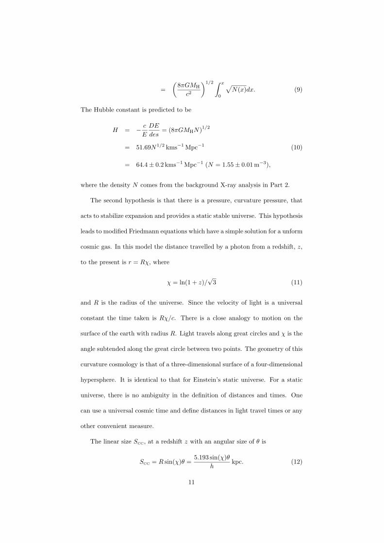
The Hubble constant is predicted to be

H = − c

E

DE

des= (8πGMHN)1/2

= 51.69N1/2 kms−1 Mpc−1 (10)

= 64.4 ± 0.2 kms−1 Mpc−1 (N = 1.55 ± 0.01m−3),

where the density N comes from the background X-ray analysis in Part 2.

The second hypothesis is that there is a pressure, curvature pressure, that

acts to stabilize expansion and provides a static stable universe. This hypothesis

leads to modified Friedmann equations which have a simple solution for a unform

cosmic gas. In this model the distance travelled by a photon from a redshift, z,

to the present is r = Rχ, where

χ = ln(1 + z)/√

3 (11)

and R is the radius of the universe. Since the velocity of light is a universal

constant the time taken is Rχ/c. There is a close analogy to motion on the

surface of the earth with radius R. Light travels along great circles and χ is the

angle subtended along the great circle between two points. The geometry of this

curvature cosmology is that of a three-dimensional surface of a four-dimensional

hypersphere. It is identical to that for Einstein’s static universe. For a static

universe, there is no ambiguity in the definition of distances and times. One

can use a universal cosmic time and define distances in light travel times or any

other convenient measure.

The linear size SCC, at a redshift z with an angular size of θ is

SCC = R sin(χ)θ =5.193 sin(χ)θ

hkpc. (12)

11

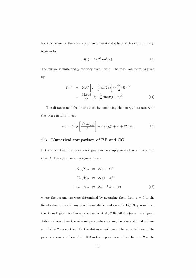
For this geometry the area of a three dimensional sphere with radius, r = Rχ,

is given by

A(r) = 4πR2 sin2(χ). (13)

The surface is finite and χ can vary from 0 to π. The total volume V , is given

by

V (r) = 2πR3

[χ − 1

2sin(2χ)

]≈ 4π

3(Rχ)3

=32.648

h3

[χ − 1

2sin(2χ)

]kpc3. (14)

The distance modulus is obtained by combining the energy loss rate with

the area equation to get

µCC = 5 log

[√3 sin(χ)

h

]+ 2.5 log(1 + z) + 42.384. (15)

2.3 Numerical comparison of BB and CC

It turns out that the two cosmologies can be simply related as a function of

(1 + z). The approximation equations are

SCC/SBB ≈ aS(1 + z)bS

VCC/VBB ≈ aV (1 + z)bV

µCC − µBB ≈ aM + bM (1 + z) (16)

where the parameters were determined by averaging them from z = 0 to the

listed value. To avoid any bias the redshifts used were for 15,339 quasars from

the Sloan Digital Sky Survey (Schneider et al., 2007, 2005, Quasar catalogue).

Table 1 shows these the relevant parameters for angular size and total volume

and Table 2 shows them for the distance modulus. The uncertainties in the

parameters were all less that 0.003 in the exponents and less than 0.002 in the

12

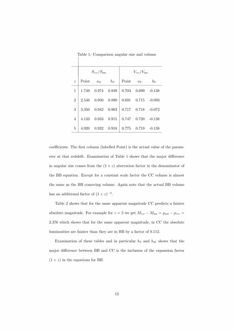
Table 1: Comparison angular size and volume

SCC/SBB VCC/VBB

z Point aS bS Point aV bV

1 1.749 0.974 0.839 0.703 0.699 -0.138

2 2.546 0.950 0.890 0.691 0.715 -0.093

3 3.350 0.942 0.903 0.717 0.718 -0.072

4 4.133 0.933 0.915 0.747 0.720 -0.138

5 4.920 0.932 0.918 0.775 0.719 -0.138

coefficients. The first column (labelled Point) is the actual value of the param-

eter at that redshift. Examination of Table 1 shows that the major difference

in angular size comes from the (1 + z) aberration factor in the denominator of

the BB equation. Except for a constant scale factor the CC volume is almost

the same as the BB comoving volume. Again note that the actual BB volume

has an additional factor of (1 + z)−3.

Table 2 shows that for the same apparent magnitude CC predicts a fainter

absolute magnitude. For example for z = 5 we get MCC − MBB = µBB − µCC =

2.376 which shows that for the same apparent magnitude, in CC the absolute

luminosities are fainter than they are in BB by a factor of 0.112.

Examination of these tables and in particular bS and bM shows that the

major difference between BB and CC is the inclusion of the expansion factor

(1 + z) in the equations for BB.

13

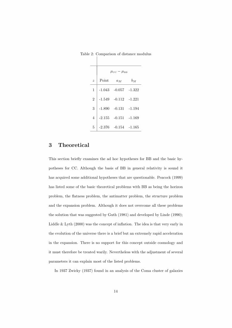
Table 2: Comparison of distance modulus

µCC − µBB

z Point aM bM

1 -1.043 -0.057 -1.322

2 -1.549 -0.112 -1.221

3 -1.890 -0.131 -1.194

4 -2.155 -0.151 -1.169

5 -2.376 -0.154 -1.165

3 Theoretical

This section briefly examines the ad hoc hypotheses for BB and the basic hy-

potheses for CC. Although the basis of BB in general relativity is sound it

has acquired some additional hypotheses that are questionable. Peacock (1999)

has listed some of the basic theoretical problems with BB as being the horizon

problem, the flatness problem, the antimatter problem, the structure problem

and the expansion problem. Although it does not overcome all these problems

the solution that was suggested by Guth (1981) and developed by Linde (1990);

Liddle & Lyth (2000) was the concept of inflation. The idea is that very early in

the evolution of the universe there is a brief but an extremely rapid acceleration

in the expansion. There is no support for this concept outside cosmology and

it must therefore be treated warily. Nevertheless with the adjustment of several

parameters it can explain most of the listed problems.

In 1937 Zwicky (1937) found in an analysis of the Coma cluster of galaxies

14

that the ratio of total mass obtained by using the virial theorem to the total

luminosity was 500 whereas the expected ratio was 3. This huge discrepancy was

the start of the concept of dark matter. It is surprising that in more than seven

decades since that time there is no direct evidence for dark matter. Similarly

the concept of dark energy (some prefer quintessence) has been introduced to

explain discrepancies in the observations of type 1a supernovae. The important

point is that these three concepts have been introduced in an ad hoc manner to

make BB fit the observations. None has any theoretical or experimental support

outside the field of cosmology.

As already stated CC is based on the hypotheses of curvature redshift and

that of curvature pressure. Both are described in Part 3 and are supported by

strong physical arguments. Curvature redshift is testable in the laboratory and

some support for curvature pressure may come from solar neutrino observations.

Nevertheless they are new hypotheses and must be subject to strong scrutiny.

4 Expansion and Evolution

The original models for BB had all galaxies being formed shortly after the be-

ginning of the universe. Then as stars aged the characteristics of the galaxies

changed. Consequently these characteristics are expected to show an evolution

that is a function of redshift. Since nearly all cosmological objects are associ-

ated with galaxies we would also expect their characteristics to show evolution.

Clearly in CC there is no evolution in the average characteristics of any ob-

ject. The individual objects will evolve but the average characteristics of the

population remain constant. Any strong evidence of evolution of the average

15

characteristics would constitute serious evidence against CC.

The simple BB evolution concept is complicated by galactic collisions and

mergers (Struck, 1999; Blanton & Moustakas, 2009). In many cases these can

produce new large star-forming regions. Clearly the influx of a large number

of new stars will alter the characteristics of the galaxy. It is likely that a sig-

nificant number of galaxies have been reformed by collisions and mergers and

consequently the average evolution may be very little or at least somewhat re-

duced over the simple model.

4.1 Tolman surface brightness

This test, suggested by Tolman (1934), relies on the observation that the sur-

face brightness of objects does not depend on the geometry of the universe.

Although it is obviously true for Euclidean geometry it is also true for non-

Euclidean geometries. For a uniform source, the quantity of light received per

unit angular area is independent of distance. However, the quantity of light is

also sensitive to non-geometric effects, which make it an excellent test to dis-

tinguish between cosmologies. For expanding universe cosmologies the surface

brightness is predicted to vary as (1 + z)−4, where one factor of (1 + z) comes

from the decrease in energy of each photon due to the redshift, another factor

comes from the decrease in rate of their arrival and two factors come from the

apparent decrease in area due to aberration. This aberration is simply the rate

of change of area for a fixed solid angle with redshift. In a static, tired-light,

cosmology (such as CC) only the first factor is present. Thus an appropriate

test for Tolman surface brightness is the value of this exponent.

16

4.1.1 Surface brightness in BB

The obvious candidates for surface brightness tests are elliptic and S0 galaxies

which have minimal projection effects compared to spiral galaxies . The major

problem is that surface brightness measurements are intrinsically difficult due to

the strong intensity gradients across their images. In a series of papers Sandage

& Lubin (2001); Lubin & Sandage (2001a,b,c) (hereafter SL01) have investigated

the Tolman surface brightness test for elliptical and S0 galaxies. More recently

Sandage (2010) has done a more comprehensive analysis but since he came to

the same conclusion as the earlier papers and since the earlier papers are better

known this analysis will concentrate on them. The observational difficulties are

thoroughly discussed by Sandage & Lubin (2001) with the conclusion that the

use of Petrosian metric radii helps solve many of the problems. Petrosian (1976);

Djorgovski & Spinrad (1981); Sandage & Perelmuter (1990) showed that if the

ratio of the average surface brightness within a radius is equal to η times the

surface brightness at that radius then that defines the Petrosian metric radius,

η. The procedure is to examine an image and to vary the angular radius until

the specified Petrosian radius is achieved.

Thus, the aim is to measure the mean surface brightness for each galaxy

at the same value of η. The choice of Petrosian radii greatly diminishes the

differences in surface brightness due to the luminosity distribution across the

galaxies. However, there still is a dependence of the surface brightness on the

size of the galaxy which is the Kormendy relationship (Kormendy, 1977). The

purpose of the preliminary analysis done by SL01 is not only to determine the

low redshift absolute luminosity but also to determine the surface brightness

verses linear size relationship that can be used to correct for effects of size

17

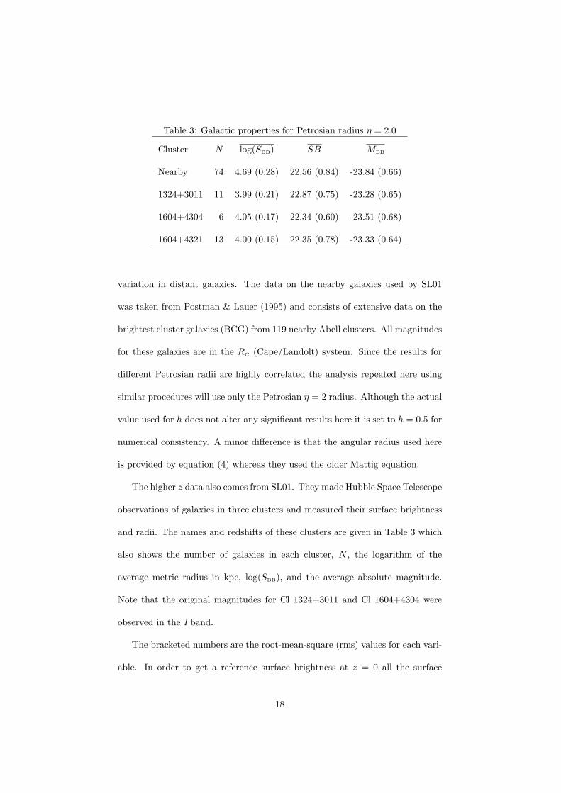
Table 3: Galactic properties for Petrosian radius η = 2.0

Cluster N log(SBB) SB MBB

Nearby 74 4.69 (0.28) 22.56 (0.84) -23.84 (0.66)

1324+3011 11 3.99 (0.21) 22.87 (0.75) -23.28 (0.65)

1604+4304 6 4.05 (0.17) 22.34 (0.60) -23.51 (0.68)

1604+4321 13 4.00 (0.15) 22.35 (0.78) -23.33 (0.64)

variation in distant galaxies. The data on the nearby galaxies used by SL01

was taken from Postman & Lauer (1995) and consists of extensive data on the

brightest cluster galaxies (BCG) from 119 nearby Abell clusters. All magnitudes

for these galaxies are in the RC (Cape/Landolt) system. Since the results for

different Petrosian radii are highly correlated the analysis repeated here using

similar procedures will use only the Petrosian η = 2 radius. Although the actual

value used for h does not alter any significant results here it is set to h = 0.5 for

numerical consistency. A minor difference is that the angular radius used here

is provided by equation (4) whereas they used the older Mattig equation.

The higher z data also comes from SL01. They made Hubble Space Telescope

observations of galaxies in three clusters and measured their surface brightness

and radii. The names and redshifts of these clusters are given in Table 3 which

also shows the number of galaxies in each cluster, N , the logarithm of the

average metric radius in kpc, log(SBB), and the average absolute magnitude.

Note that the original magnitudes for Cl 1324+3011 and Cl 1604+4304 were

observed in the I band.

The bracketed numbers are the root-mean-square (rms) values for each vari-

able. In order to get a reference surface brightness at z = 0 all the surface

18

brightness values, SB, of the nearby galaxies were reduced to absolute surface

brightnesses by using Eq. 17. Since all the redshifts are small, this reduction

is essentially identical for all cosmological models. However the calculation of

the metric radii for the distant galaxies is very dependent on the cosmological

model. This procedure of using the BB in analyzing a test of BB is discussed

in SL01. Their conclusion is that it reduces the significance of a positive result

from being strongly supportive to being consistent with the model. Of interest

is that Table 3 shows that on average the distant galaxies are smaller than the

nearby galaxies.

Then a linear least squares fit of the absolute surface brightness as a function

of log(SBB), the Kormendy relationship, for the nearby galaxies results in the

equation

SB = 9.29 ± 0.50 + (2.83 ± 0.11) log(SBB) (17)

whereas SL01 found a slightly different equation

SB = 8.69 ± 0.06 + (2.97 ± 0.05) log(SBB). (18)

Although a small part of the discrepancy is due to slightly different proce-

dures the main reason for the discrepancy is unknown. Of the 74 galaxies used

there were 19 that had extrapolated estimates for either the radius or the surface

brightness or both. In addition there were only three galaxies that differed from

the straight line by more than 2σ. They were A147 (2.9σ), A1016 (2.0σ)and

A3565 (-2.4σ). omission of all or some of these galaxies did not improve the

agreement. The importance of this preliminary analysis is that Eq. 17 contains

all the information that is needed from the nearby galaxies in order to calibrate

the distant cluster galaxies.

19

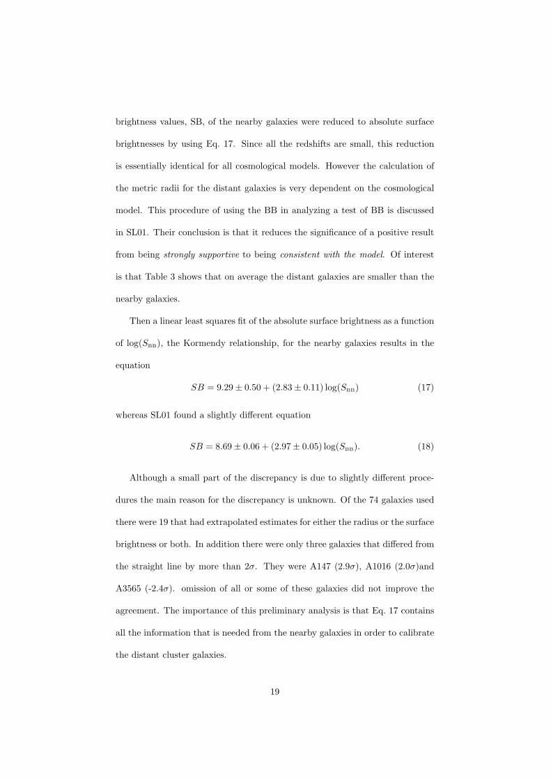
Table 4: Fitted exponents for distant clusters (η = 2.0)

Cluster Col z nBB nSL01

1324+3011 I 0.757 1.98±0.19 1.99±0.15

1604+4304 I 0.897 2.22±0.22 2.29±0.21

1604+4321 R 0.924 2.24±0.18 2.48±0.25

Next we use the galaxies’ radius and Eq. 17 to correct the apparent sur-

face brightness of the distant galaxies for the Kormendy relation and then do

least squares fit to the difference between the corrected surface brightness and

its absolute surface brightness as a function of 2.5 log(1 + z) to estimate the

exponent, n, where SB ∝ (1 + z)n. If needed the non-linear corrections given

by Sandage (2010) were applied to the nearby surface brightness values. For

the I band galaxies the absolute surface brightness included the color correction

< R−I >= 0.62 Lubin & Sandage (2001c). The results for the exponent, n, for

each cluster are shown in Table 4 together with the values from SL01 (column 5)

where the second column is the band (color) in which the cluster was observed.

Because the definition of magnitude contains a negative sign the expected

value for n in BB is four. Nearly all of the difference between these results

and those from SL01 arises from the use of a different Kormendy relationship.

If the Kormendy relationship used by SL01 (Eq. 18 is used instead of Eq. 17)

the agreement is excellent. If it is assumed that there is no evolutionary or

other differences between the three clusters and all the data are combined the

resulting exponent is nBB = 2.16 ± 0.13.

Clearly there is a highly significant disagreement between the observed ex-

ponents and the expected exponent of four. Both SL01 and Sandage (2010)

20

claim that the difference is due to the effects of luminosity evolution. Based on

a range of theoretical models SL01 show that the amount of luminosity evolu-

tion expressed as the exponent, p = 4−nBB, varies between p =0.85–2.36 in the

R band and p =0.76–2.07 in the I band. In conclusion to their analysis they

assert that they have either (1) detected the evolutionary brightening directly

from the SB observations on the assumption that the Tolman effect exists or

(2) confirmed that the Tolman test for the reality of the expansion is positive,

provided that the theoretical luminosity correction for evolution is real.

SL01 also claim that their results are completely inconsistent with a tired

light cosmology. Although this is explored for CC in the next sub-section it is

interesting to consider a very simple model. The essential property of a tired

light model is that it does not include the time dilation factor of (1 + z) in its

angular radius equation. Thus assuming BB but without the (1 + z) term all

values of log(SBB) will be increased by log(1 + z). Hence the predicted absolute

surface brightness will be (numerically) increased by (2.83/2.5)log(1 + z). For

example, the exponent for all clusters will be changed to

ntired light = 2.16 ± 0.16 − 2.832.5

= 1.03 ± 0.16

This is clearly close to the expected value of unity predicted by a tired-light

cosmology and thus disagrees with the conclusion of SL01 that the data are

incompatible with a tired light cosmology.

There are two major criticisms of this work. The first is that relying on

theoretical models to cover a large gap between the expected index and the

measured index makes the argument very weak. Although SL01 indirectly con-

sider the effects of relatively common galaxy interactions and mergers in the

very wide estimates they provide for the evolution, the fact that there is such a

21

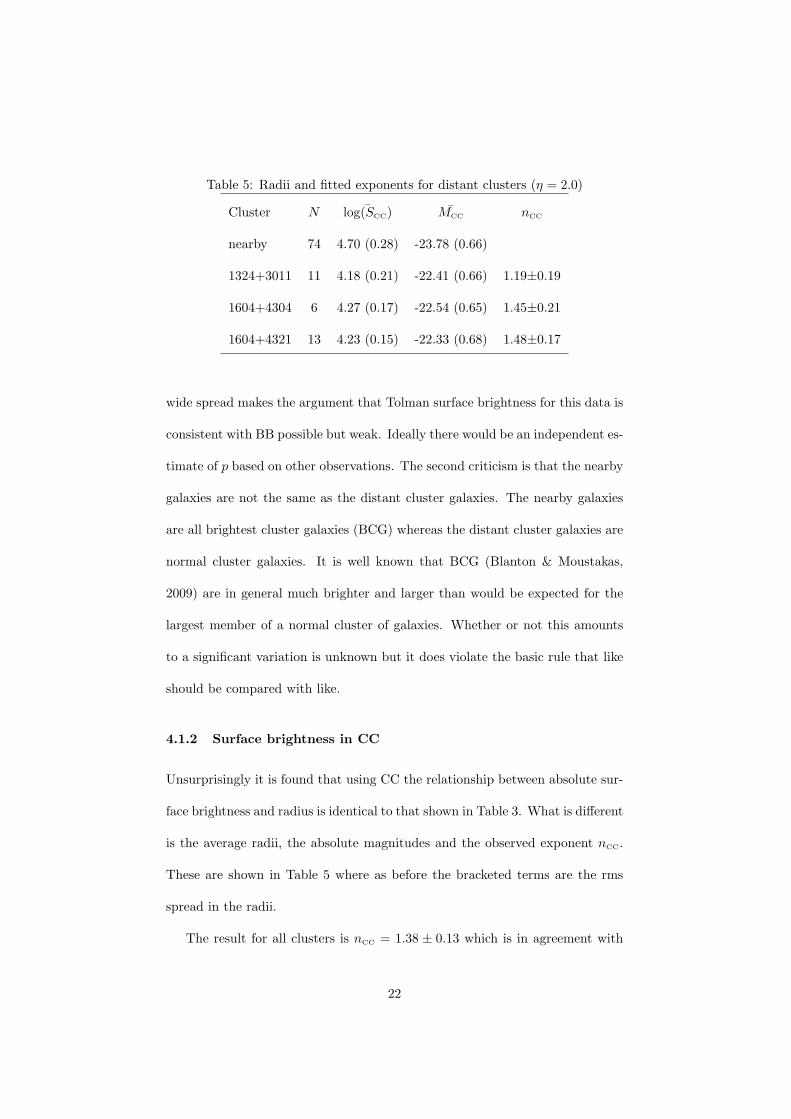
Table 5: Radii and fitted exponents for distant clusters (η = 2.0)

Cluster N ¯log(SCC) MCC nCC

nearby 74 4.70 (0.28) -23.78 (0.66)

1324+3011 11 4.18 (0.21) -22.41 (0.66) 1.19±0.19

1604+4304 6 4.27 (0.17) -22.54 (0.65) 1.45±0.21

1604+4321 13 4.23 (0.15) -22.33 (0.68) 1.48±0.17

wide spread makes the argument that Tolman surface brightness for this data is

consistent with BB possible but weak. Ideally there would be an independent es-

timate of p based on other observations. The second criticism is that the nearby

galaxies are not the same as the distant cluster galaxies. The nearby galaxies

are all brightest cluster galaxies (BCG) whereas the distant cluster galaxies are

normal cluster galaxies. It is well known that BCG (Blanton & Moustakas,

2009) are in general much brighter and larger than would be expected for the

largest member of a normal cluster of galaxies. Whether or not this amounts

to a significant variation is unknown but it does violate the basic rule that like

should be compared with like.

4.1.2 Surface brightness in CC

Unsurprisingly it is found that using CC the relationship between absolute sur-

face brightness and radius is identical to that shown in Table 3. What is different

is the average radii, the absolute magnitudes and the observed exponent nCC.

These are shown in Table 5 where as before the bracketed terms are the rms

spread in the radii.

The result for all clusters is nCC = 1.38 ± 0.13 which is in agreement with

22

unity. Note that the critical difference from BB is in the size of the radii. They

are not only much closer to the nearby galaxy radii but because they are larger

they do not require the non-linear corrections for the Kormendy relation. As

before we note that the nearby galaxies are BCG which may have a brighter

SB than the normal field galaxies. If this is true it would bias the exponent

to a larger value. If we assume that CC is correct then this data shows that

on average the BCG galaxies are −0.64 ± 0.08 mag (which is a factor of 1.8 in

luminosity) brighter than the general cluster galaxies.

4.1.3 Conclusion for surface brightness

The SL01 data for the surface brightness of elliptic galaxies is consistent with

BB but only if a large unknown effect of luminosity evolution is included. The

data do not support expansion and are in complete agreement with CC.

4.2 Angular size

Closely related to surface brightness is relationship between the observed angu-

lar size of a distant object and its actual linear transverse size. The variation

of angular size as a function of redshift is one of the tests that should clearly

distinguish between BB and CC. The major distinction is that CC like all tired-

light cosmologies does not include the (1+ z) aberration factor. Its relationship

(Eq. 12) between the observed angular size and the linear size is very close (for

small redshifts) to the Euclidean equation. Gurvits, Kellermann & Frey (1999)

provide a comprehensive history of studies for a wide range of objects that gen-

erally show a 1/z or Euclidean dependence. Most observers suggest that the

probable cause is some form of size evolution. Recently Lopez-Corredoira (2010)

23

used 393 galaxies with redshift range of 0.2 < z < 3.2 in order to test many

cosmologies. Briefly his conclusions are

The average angular size of galaxies is approximately proportional to z−α with

α between 0.7 and 1.2.

Any model of an expanding universe without evolution is totally unable to fit

the angular size data . . .

Static Euclidean models with a linear Hubble law or simple tired-light fit the

shape of the angular size vs z dependence very well: there is a difference

in amplitude of 20%–30%, which is within the possible systematic errors.

It is also remarkable that the explanation of the test results with an expanding

model require four coincidences:

1. The combination of expansion and (very strong evolution) size evolu-

tion gives nearly the same result as a static Euclidean universe with

a linear Hubble law: θ ∝ z−1.

2. This hypothetical evolution in size for galaxies is the same in normal

galaxies as in quasars, as in radio galaxies, as in first ranked cluster

galaxies, as the separation among bright galaxies in cluster

3. The concordance (ΛCDM) model gives approximately the same (dif-

ferences of less than 0.2 mag within z < 4.5) distance modulus in a

Hubble diagram as the static Euclidean universe with a linear law.

4. The combination of expansion, (very strong) size evolution, and dark

matter ratio variation gives the same result for the velocity dispersion

in elliptical galaxies (the result is that it is nearly constant with z)

24

as for a simple static model with no evolution in size and no dark

matter ratio variation.

With a redshift range of z < 3 the value of SCC is approximately proportional

to z0.68 which shows that it is consistent with these results. A full analysis re-

quires a fairly complicated procedure to correct the observed sizes for variations

in the absolute luminosity.

A simple example of the angular size test can be done using double-lobed

quasars. Using quasar catalogues, Buchalter et al. (1998) carefully selected

103 edge-brightened, double-lobed sources from the VLA FIRST survey and

measured their angular sizes directly from the FIRST radio maps. These are

Faranoff-Riley type II objects (Fanaroff & Riley, 1974) and exhibit radio-bright

hot-spots near the outer edges of the lobes. Since Buchalter et al. (1998) claim

that three different Friedmann (BB) models fit the data well but that a Eu-

clidean model had a relatively poor fit a re-analysis is warranted. The angular

sizes were converted to linear sizes for each cosmology and were divided into

six bins so that there were 17 quasars in each bin. Because these double-lobed

sources are essentially one dimensional a major part of their variation in size is

due to projection effects. For the moment assume that in each bin they have

the same size, S, and the only variation is due to projection then the observed

size is S sin(θ) where θ is the projection angle. Clearly we do not know the

projection angle but we can assume that all angles are equally likely so that if

the N sources, in each bin, are sorted into increasing size the i’th source in this

list should have, on average, an angle θi = π(2i − 1)/4N . Thus the maximum

25

likelihood estimate of S is

Sest =∑N

i=1 sin(θi)Si∑Ni=1 sin2(θi)

.

Note that the sum in the denominator is a constant and that the common

procedure of using median values is the same as using only the central term

in the sum. Next a regression (Section A) was done between logarithm of the

estimated linear size in each bin and log(1 + z) where z is the mean redshift.

Then the significance of the test was how close was the exponent, b, to zero.

For BB the exponent was b = −0.79 ± 0.44 and for CC it was b = 0.16 ± 0.44.

Although the large uncertainties show that this is not a decisive discrimination

between the two cosmologies the slope for BB suggests that no expansion is

likely. The overall conclusion is strongly in favor of no expansion.

4.3 Type 1a supernovae

Type 1a supernovae make ideal cosmological probes. Nearby observations show

that they have an essentially constant peak absolute magnitude and the widths

of the light curves provide an ideal probe to investigate the dependence of time

delay as a function of redshift. The current model for type 1a supernovae

(Hillebrandt & Niemeyer, 2000) is that of a white dwarf steadily acquiring mat-

ter from a close companion until the mass exceeds the Chandrasekhar limit

at which point it explodes. The light curve has a rise time of about 20 days

followed by a fall of about 20 days and then a long tail that is most likely

due to the decay of 56Ni. The widths are measured in the light coming from

the expanding shells before the radioactive decay dominates. Thus the widths

are a function of the structure and opacity of the initial explosion and have

little dependence on the radioactive decay. The type 1a supernovae are distin-

26

guished from other types of supernovae by the absence of hydrogen lines and

the occurrence of strong silicon lines in their spectra near the time of maximum

luminosity. Although the theoretical modeling is poor, there is much empirical

evidence, from nearby supernovae, that they all have remarkably similar light

curves, both in absolute magnitude and in their time scales. This has led to a

considerable effort to use them as cosmological probes. Since they have been

observed out to redshifts with z greater than one they have been used to test

the cosmological time dilation that is predicted by expanding cosmologies.

Several major projects have used both the Hubble space telescope and large

earth-bound telescopes to obtain a large number of type 1a supernova obser-

vations, especially to large redshifts. They include the Supernova Cosmology

Project (Perlmutter et al., 1999; Goldhaber et al., 2001; Knop et al., 2003), the

Supernova Legacy Survey (Astier et al., 2005), the Hubble Higher z supernovae

Search (Strolger et al., 2004) and the ESSENCE supernova survey (Wood-Vasey

et al., 2008; Davis et al., 2007). Recently Kowalski et al. (2008) have provided

a re-analysis of these survey data and all other relevant supernovae in the liter-

ature and have provided new observations of some nearby supernovae. Because

these Union data are comprehensive, uniformly analyzed and include nearly all

previous observations, the following analysis will be confined to this data. The

data provided (Bessel) B-band magnitudes, stretch factors, and B − V colors

for supernovae in the range 0.015 6 z 6 1.551. Since there is a very small

but significant dependence of the absolute magnitude on the B − V color , in

effect the K-correction, following Kowalski et al. (2008) the magnitudes were

reduced by a term β(B − V ) where β was determined by minimizing the χ2 of

the residuals after fitting MBB verses 2.5 log(1 + z). This gave β = 1.54 which

27

can be compared with β = 2.28 given by Kowalski et al. (2008).

The widths (relative to the standard width), w, of the supernova light curves

are derived from the stretch factors, s, provided by Kowalski et al. (2008) by the

equation w = (1 + z)s. The uncertainty in each width was taken to be (1 + z)

times the quoted uncertainty in the stretch value. For convenience in determin-

ing power law exponents a new variable W is defined by W = 2.5 log(w). Since

the width is relative to a standard template the reference value for W is W0 = 0.

Fig. 1 shows a plot of these widths as a function of redshift. An preliminary fit

for W as a function of 2.5 log(1+z) showed an offset −0.095±0.014. This offset

was removed from the supernova widths, W , before further analysis was done.

The same color correction and width offset will be used for both cosmologies.

What is relevant for both cosmologies is the selection procedure. The cur-

rent technique for the supernova observations is a two-stage process (Perlmutter

& Schmidt, 2003; Strolger et al., 2004; Riess et al., 2004). The first stage is to

conduct repeated observations of many target areas to look for the occurrence

of supernovae. Having found a possible candidate the second stage is to con-

duct extensive observations of magnitude and spectra to identify the type of

supernova and to measure its light curve. This second stage is extremely ex-

pensive of resources and it is essential to be able to determine quickly the type

of the supernova so that the maximum yield of type 1a supernovae is achieved.

Since current investigators assume that the type 1a supernovae have essentially

a fixed absolute BB magnitude (with possible corrections for the stretch factor),

one of the criteria they used is to reject any candidate whose predicted abso-

lute peak magnitude is outside a rather narrow range. The essential point is

that the absolute magnitudes are calculated using BB and hence the selection

28

of candidates is dependent on the BB luminosity-distance modulus. In a com-

prehensive description of the selection procedure for a major survey Strolger et

al. (2004) state: Best fits required consistency in the light curve shape and peak

color (to within magnitude limits) and in peak luminosity in that the derived

absolute magnitude in the rest-frame B band had to be consistent with observed

distribution of absolute B-band magnitudes shown in Richardson et al. (2002).

4.3.1 Supernovae in BB

Fundamental to any cosmology that explains the Hubble redshift as being due

to an expanding universe is the requirement that exactly the same dependence

must apply to time dilation. The raw data of the widths of the type 1a su-

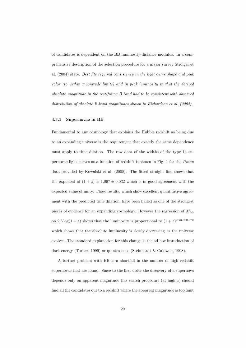
pernovae light curves as a function of redshift is shown in Fig. 1 for the Union

data provided by Kowalski et al. (2008). The fitted straight line shows that

the exponent of (1 + z) is 1.097 ± 0.032 which is in good agreement with the

expected value of unity. These results, which show excellent quantitative agree-

ment with the predicted time dilation, have been hailed as one of the strongest

pieces of evidence for an expanding cosmology. However the regression of MBB

on 2.5 log(1 + z) shows that the luminosity is proportional to (1 + z)0.230±0.070

which shows that the absolute luminosity is slowly decreasing as the universe

evolves. The standard explanation for this change is the ad hoc introduction of

dark energy (Turner, 1999) or quintessence (Steinhardt & Caldwell, 1998).

A further problem with BB is a shortfall in the number of high redshift

supernovae that are found. Since to the first order the discovery of a supernova

depends only on apparent magnitude this search procedure (at high z) should

find all the candidates out to a redshift where the apparent magnitude is too faint

29

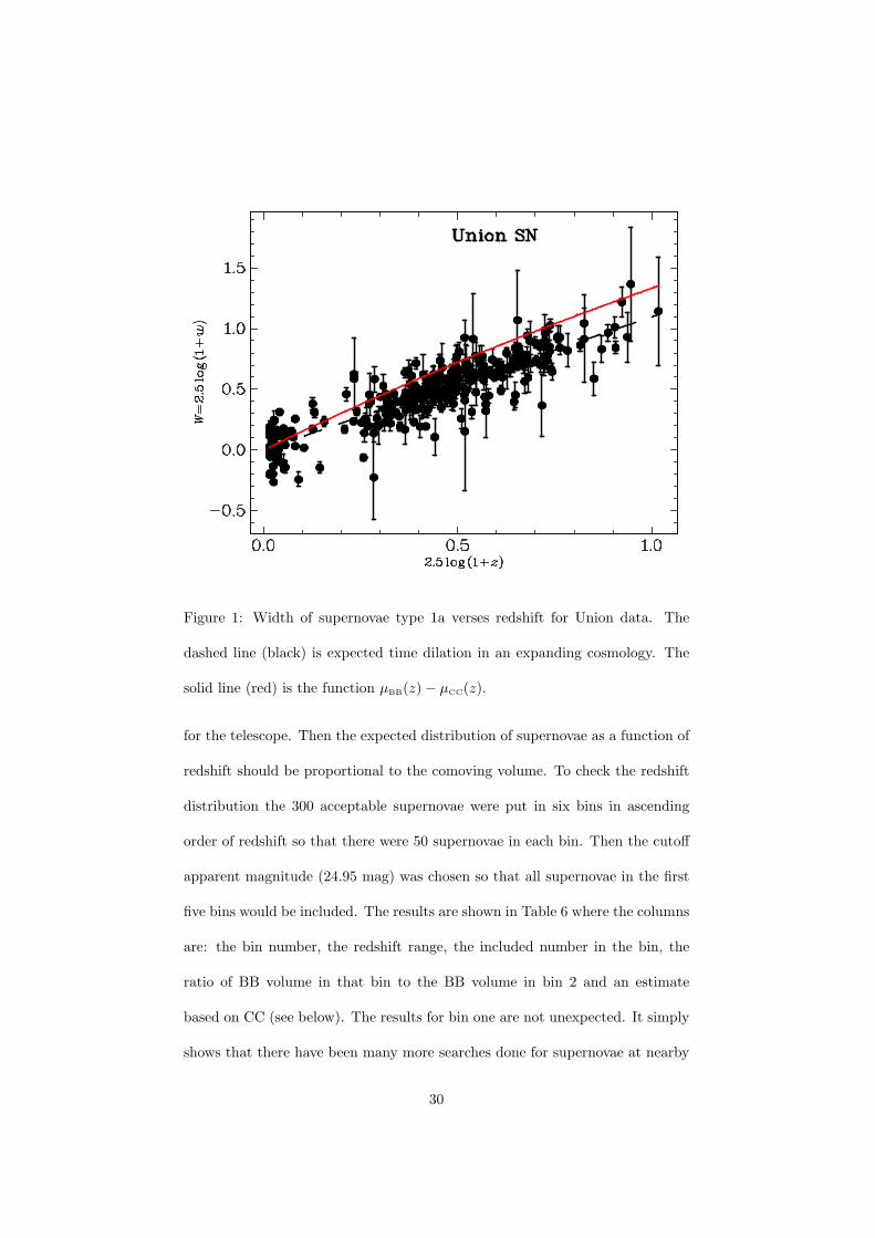
Figure 1: Width of supernovae type 1a verses redshift for Union data. The

dashed line (black) is expected time dilation in an expanding cosmology. The

solid line (red) is the function µBB(z) − µCC(z).

for the telescope. Then the expected distribution of supernovae as a function of

redshift should be proportional to the comoving volume. To check the redshift

distribution the 300 acceptable supernovae were put in six bins in ascending

order of redshift so that there were 50 supernovae in each bin. Then the cutoff

apparent magnitude (24.95 mag) was chosen so that all supernovae in the first

five bins would be included. The results are shown in Table 6 where the columns

are: the bin number, the redshift range, the included number in the bin, the

ratio of BB volume in that bin to the BB volume in bin 2 and an estimate

based on CC (see below). The results for bin one are not unexpected. It simply

shows that there have been many more searches done for supernovae at nearby

30

Table 6: Density distribution

bin z range Nbin VolBBa psVCC

b

1 0.014–0.123 50 0.04 0.10

2 0.123–0.387 50 1.00 1.00

3 0.387–0.495 50 0.89 0.49

4 0.495–0.612 50 1.29 0.43

5 0.612–0.821 50 3.09 0.51

6 0.821–1.560c 33 d 6.40 0.37

aThe ratio of volumes in BB: VBB(n)/VBB(2)

bThe ratio of selection probability times CC volume

cRedshift range used columns 4 and 5 is 0.821–1.139

dThe number brighter than the cutoff of 24.95 mag

redshifts. The results for bin six show that 33 out of 50 supernovae had an

apparent magnitude brighter than the cut-off. To compensate the volume for

bin 6 was computed for a redshift limit of z = 1.139 which was the highest

redshift for an included supernova. The problem with the BB results is that

there is a dramatic shortage of supernovae in the high redshift bins. The usual

explanation is that this shortage is due to evolutionary effects. However this

explanation must be able to show why there is a dramatic decrease in the rate

of occurrence of supernovae at redshifts for z near one when there is no obvious

change in the stellar contents of galaxies with these redshifts.

31

4.3.2 Supernovae in CC

Since the redshift in CC arises from an interaction with the intervening gas, it

is not always a good measurement of distance. In particular the halo around

our galaxy and that around any target galaxy will produce an extra redshift

that results in an overall redshift that is larger than would be expected from the

distance and a constant inter-galactic gas density. Since this is an additive effect

it is important only for nearby objects. In fact the nearby supernovae (defined

as those with z < 0.15) show an average absolute magnitude that is brighter

than the extrapolated magnitude from more distant supernovae. In order to

make a partial correction for this bias all redshifts were reduced by subtracting

0.006 from each redshift, z. This correction brought the near and more distant

magnitudes into agreement. A plot of absolute magnitude, MCC, verses width,

W , is shown in Fig. 2. For later analysis the data are divided into the same 6

redshift bins used in Table 6. The best-fit straight line to all the supernova has a

(global) slope of 0.695± 0.072 (for MBB it is −0.391± 0.056). This implies that

supernovae that are brighter have narrower widths, or the weaker are wider.

Table 7 gives the rms of the reduced magnitudes and the slope of the reduced

magnitudes verses the width, W , for each bin. However Phillips (1993); Hamuy

et al. (1996); Guy et al. (2005) argue for a local dependence of magnitude on

stretch that has the opposite sign to the fitted straight line.

In the first bin the stretch and magnitude are essentially identical so that

we can compare the local result of −1.19 ± 0.21 with −1.56 ± 0.25 reported by

Guy et al. (2005) to show good agreement. The slope for the other bins shows

that although this local slope is not so well defined it is clearly present at higher

redshifts. The challenge is to explain why the slope in a small redshift range is

32

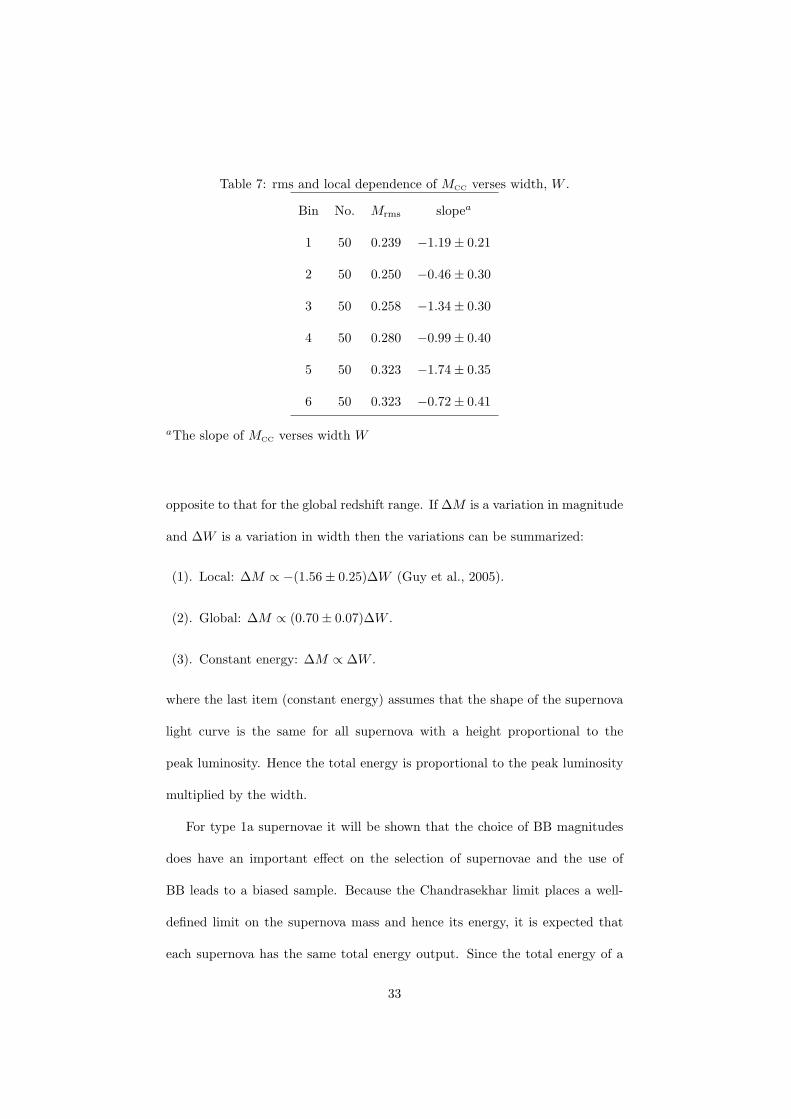
Table 7: rms and local dependence of MCC verses width, W .

Bin No. Mrms slopea

1 50 0.239 −1.19 ± 0.21

2 50 0.250 −0.46 ± 0.30

3 50 0.258 −1.34 ± 0.30

4 50 0.280 −0.99 ± 0.40

5 50 0.323 −1.74 ± 0.35

6 50 0.323 −0.72 ± 0.41

aThe slope of MCC verses width W

opposite to that for the global redshift range. If ∆M is a variation in magnitude

and ∆W is a variation in width then the variations can be summarized:

(1). Local: ∆M ∝ −(1.56 ± 0.25)∆W (Guy et al., 2005).

(2). Global: ∆M ∝ (0.70 ± 0.07)∆W .

(3). Constant energy: ∆M ∝ ∆W .

where the last item (constant energy) assumes that the shape of the supernova

light curve is the same for all supernova with a height proportional to the

peak luminosity. Hence the total energy is proportional to the peak luminosity

multiplied by the width.

For type 1a supernovae it will be shown that the choice of BB magnitudes

does have an important effect on the selection of supernovae and the use of

BB leads to a biased sample. Because the Chandrasekhar limit places a well-

defined limit on the supernova mass and hence its energy, it is expected that

each supernova has the same total energy output. Since the total energy of a

33

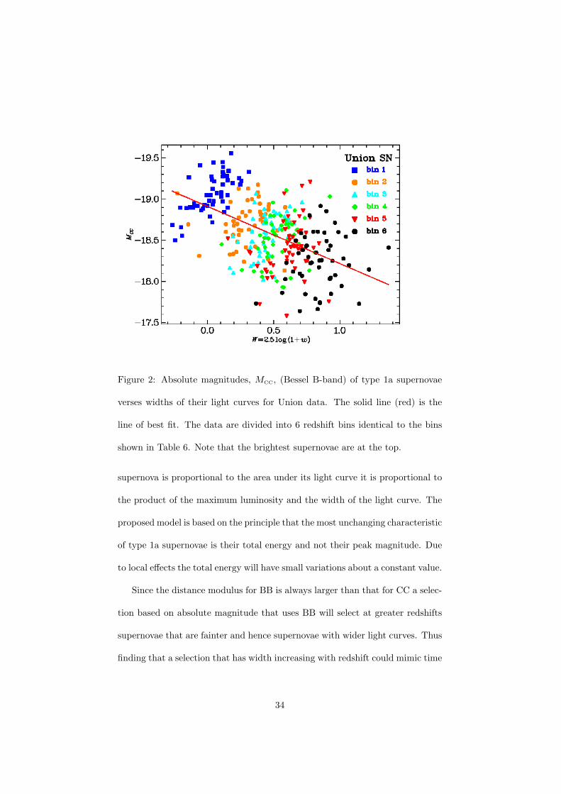
Figure 2: Absolute magnitudes, MCC, (Bessel B-band) of type 1a supernovae

verses widths of their light curves for Union data. The solid line (red) is the

line of best fit. The data are divided into 6 redshift bins identical to the bins

shown in Table 6. Note that the brightest supernovae are at the top.

supernova is proportional to the area under its light curve it is proportional to

the product of the maximum luminosity and the width of the light curve. The

proposed model is based on the principle that the most unchanging characteristic

of type 1a supernovae is their total energy and not their peak magnitude. Due

to local effects the total energy will have small variations about a constant value.

Since the distance modulus for BB is always larger than that for CC a selec-

tion based on absolute magnitude that uses BB will select at greater redshifts

supernovae that are fainter and hence supernovae with wider light curves. Thus

finding that a selection that has width increasing with redshift could mimic time

34

dilation.

Define the magnitude of the total energy, E, in the same way as the magni-

tude of the luminosity, that is E = −2.5 log(E/E′) where E′ is a reference energy.

Then the first assumption is that although individual supernovae will show vari-

ation in total energy, magnitude and width we expect that the averages over

many supernovae will satisfy the equation E = M − W . Since, by definition,

the reference width, W0, is zero the expected value of the energy is E0 = M0

where M0 is the reference magnitude. Since its expected value is constant E

will be a better standard candle than M .

To summarize, by relying on BB distance modulus the (distant) supernovae

search method consistently selects supernova that are weaker than expected.

This pushes the selection towards the limits of the natural variation and also

selects supernovae with wider light curves. If the error in the BB magnitudes

is due to the inclusion of the time dilation term the correct absolute luminosity

is smaller than the BB luminosity by a factor of (1 + z). Thus with constant

energy, the width is larger by a factor of (1 + z) which agrees with the results

shown in Fig. 1.

Using CC and a constant energy model the dependence is ∆M = MBB −

MCC = µCC − µBB we get ∆W = µBB − µCC which is shown as the solid (red)

line in Fig. 1. Considering that the selected supernovae are a biased sample the

agreement with the widths is reasonable. There is still a problem of explaining

the local slope. In BB the average of the local slope over the six bins is −1.24±

0.15 compared with the global slope of −0.391 ± 0.056 and for CC the average

local slope is −1.07 ± 0.20. Consider a supernovae with above average energy.

If the only change in the shape of the light curve is a larger scaling factor the

35

the peak luminosity will be proportional the the width which agrees with the

average local slope.

Finally this model can be used to get an approximate estimate of the ex-

pected number of supernovae that would be selected. The nearby supernovae

come from a wide range of heterogenous surveys and serendipitous observa-

tions. Consequently their selection probability is essentially unknown. However

the more recent, distant supernovae come from deliberate surveys that scan a

small area of the sky looking for sudden outbursts. The crucial point is that

provided the apparent magnitude of the supernova is within the observational

constraints the probability of detection is independent of redshift. Thus as a

first approximation all the surveys may be combined in order to determine the

expected number of supernovae that should be detected.

Assuming that the intrinsic distribution in magnitude is normal (with a stan-

dard deviation of σ) and that a supernova is selected if MBB falls with a narrow

range about the reference value, then the probability of selection is proportional

to exp(−(µBB(z) − µCC(z))2/2σ2). The test is whether the number of expected

supernovae as a function of redshift is similar to the observed number. The ex-

pected numbers (probability times volume, VCC), are shown for σ = 0.37 in the

last column of Table 6. Note that the redshift ranges for each bin are determined

by the observed supernovae which are heavily biased in bin 1 and probably also

in bin 2 due to the inclusion of supernovae from many local surveys that do

not fit the selection model. Consequently the value of σ = 0.35 was chosen to

provide roughly equal values for bins 3, 4 and 5. The average of the rms of MCC

shown in Table 7 is 0.32 mag which is reasonably consistent with σ = 0.37.

It has been argued that the total energy of type 1a supernovae makes a good

36

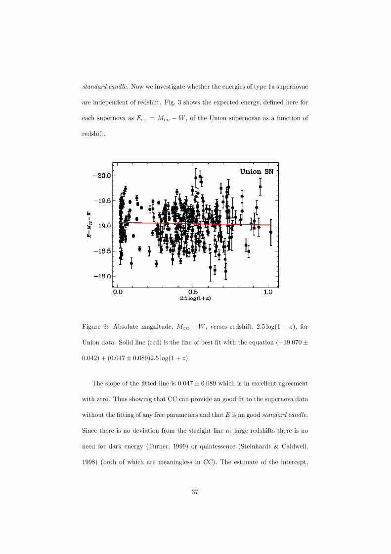
standard candle. Now we investigate whether the energies of type 1a supernovae

are independent of redshift. Fig. 3 shows the expected energy, defined here for

each supernova as ECC = MCC − W , of the Union supernovae as a function of

redshift.

Figure 3: Absolute magnitude, MCC − W , verses redshift, 2.5 log(1 + z), for

Union data. Solid line (red) is the line of best fit with the equation (−19.070±

0.042) + (0.047 ± 0.089)2.5 log(1 + z)

The slope of the fitted line is 0.047 ± 0.089 which is in excellent agreement

with zero. Thus showing that CC can provide an good fit to the supernova data

without the fitting of any free parameters and that E is an good standard candle.

Since there is no deviation from the straight line at large redshifts there is no

need for dark energy (Turner, 1999) or quintessence (Steinhardt & Caldwell,

1998) (both of which are meaningless in CC). The estimate of the intercept,

37

that is M0, is −19.070 ± 0.042. Riess et al. (2005) have measured accurate

distances to two galaxies containing nearby supernovae. Together with two

earlier measurements, they derive an absolute magnitude of type 1a supernovae

of −19.17±0.07. Hence the reduced Hubble constant, h, can be estimated from

−19.070 − 5 log(0.7) = −19.17 − 5 log(h) to get h = 0.638 ± 0.05. Thus the

measured Hubble constant is 63.8 ± 0.5 kms−1 Mpc−1.

4.3.3 Supernova conclusion

It has been shown that there is very strong support for the proposition that

the most invariant property of type 1a supernovae is their total energy and

not their peak magnitude. Given an essentially constant energy there is an

inverse relationship between the peak luminosity and the width of the light

curve. Since the prime characteristic used for selecting these supernovae is

the peak magnitude which is computed using BB there is a strong bias that

results in intrinsically weaker supernovae being selected at higher redshifts. For

constant energy these weaker supernovae must have wider light curves. Using a

simple model for the selection process it was shown that it predicts the observed

dependence for the light curve widths on redshift (Fig. 1). It is also consistent

with the observed local variation of magnitudes on widths. When the observed

magnitudes are corrected for the supernova width, they are independent of

redshift (Fig. 3). The conclusion is that with a simple selection model these

supernovae observations are fully compatible with CC and there is no need for

dark energy or quintessence. This is strong support for the premise that there

is no time dilation and hence no universal expansion.

38

4.4 Gamma ray bursts (GRB)

Gamma-Ray bursts (GRB) are transient events with time scales of the order

of seconds and with energies in the X-ray or gamma-ray region. Piran (2004)

provides (a mainly theoretical) review and Bloom, Frail & Kulkarni (2003) give

a review of observations and analysis. Although the reviews by Meszaros (2006)

and Zhang (2007) cover more recent research and provide extensive references

they are mainly concerned with GRB models. This paper considers only the

direct GRB observations and makes no assumptions about GRB models.

The search for the time dilation signature in data from GRB has a long his-

tory and before redshifts were available Norris et al. (1994); Fenimore & Bloom

(1995); Davis et al. (1994) claimed evidence for a time dilation effect by compar-

ing dim and bright bursts. However Mitrofanov et al. (1996) found no evidence

for time dilation. Lee, Bloom & Petrosian (2000) found rather inconclusive re-

sults from a comparison between brightness measures and timescale measures.

They also provide a brief summary of earlier results. Since redshifts have become

available Chang (2001) and Chang, Yoon & Choi (2002) using a Fourier energy

spectrum method and Borgonovo (2004) using an autocorrelation method claim

evidence of time dilation. The standard understanding, starting with Norris

(2002) and Bloom et al. (2003), is that time dilation is present but because of

an inverse relationship between luminosity and time measures it cannot be seen

in the raw data. Their argument is that because a strong luminosity-dependent

selection produces an average luminosity that increases with redshift there will

be a simultaneous selection for time measures that decrease with redshift which

can cancel the effects of time dilation.

Crawford (2009b) has argued that within the paradigm of BB that there is no

39

evidence for strong luminosity selection or luminosity evolution. Consequently

those time measures that show a strong relationship with luminosity must have

evolved in a similar manner. Although it is possible that a combination of

luminosity selection, selection of GRB by other characteristics and evolution

may be sufficient to cancel time dilation it does require a fortuitous coincidence

of these effects to completely cancel the effects of time dilation in the raw data.

Another explanation is that the universe is not expanding and thus there is no

time dilation.

4.5 Galaxy distribution

Recently, large telescopes with wide fields and the use of many filters have

enabled a new type of galactic survey. The light-collecting capability of the large

telescopes enables deep surveys to apparent magnitudes of 24 mag or better and

the wide field provides a fast survey over large areas. A major innovation is the

use of many filters whose response can be used to classify the objects with

great accuracy. Thus, galaxies can be separated from quasars without needing

morphological analysis. This photometric method of analysis works because

photometric templates are available for a wide range of types of galaxies and

other types of objects. In addition, accurate redshifts are obtained from fitting

the templates without the tedious procedure of measuring the spectrum of each

object.

A typical example of this photometric method is the COMBO-17 survey

(Classifying Objects by Medium-Band Observations in 17 filters) provided by

Wolf et al. (2004). The goal of this survey was to provide a sample of 50,000

galaxies and 1000 quasars with rather precise photometric redshifts based on

40

17 colors. In practice, such a filter set provides a redshift accuracy of 0.03 for

galaxies and 0.1 for quasars. The central wavelength of the 17 filters varied

from 364 nm to 914 nm and consisted of 5 broadband filters (U,B, V,R, andI)

and 12 narrower-band filters. Wolf et al. (2003) have analyzed this data and

claim that there is strong evolution for 0.2 < z < 1.2. Instead of using generic

K-corrections, the restframe luminosity of all galaxies are individually measured

from their 17-filter spectrum. For each galaxy, three restframe passbands are

considered, (i) the SDSS r-band, (ii) the Johnston B-band and (iii) a syn-

thetic UV continuum band centered at λrest= 280 nm with 40 nm FWHM and

rectangular transmission function. A spectral energy distribution, SED, was

determined for each galaxy by template matching. For the evolution analysis

they were assigned to one of four types. The only type that showed a well de-

fined peak in their luminosity distribution was Type 1 which covers the E-Sa

galactic types. The characteristics of the luminosity distribution were obtained

by fitting a Schechter function which is

ϕ(L)dLϕ∗(L/L∗)αeL/L∗dL

where the luminosity L∗ (and its magnitude M∗) is a measure of location and

α is a measure of shape. They found that a fixed value for α works quite well

for the luminosity functions of individual SED types. Examination of their

estimate of M∗ for Type 1 galaxies showed that if they were converted to CC

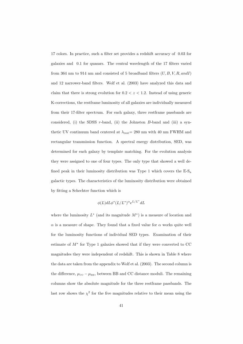
magnitudes they were independent of redshift. This is shown in Table 8 where

the data are taken from the appendix to Wolf et al. (2003). The second column is

the difference, µCC −µBB, between BB and CC distance moduli. The remaining

columns show the absolute magnitude for the three restframe passbands. The

last row shows the χ2 for the five magnitudes relative to their mean using the

41

Table 8: M∗CC for SED Type 1 galaxy luminosity distributions.

z ∆µ M∗r

a M∗B M∗

280

0.3 0.426 -20.49 -19.06 -17.38

0.5 0.642 -20.49 -19.15 -17.84

0.7 0.822 -20.77 -19.37 -17.62

0.9 0.975 -20.54 -19.09 -17.79

1.1 1.107 -20.87 -19.23 -18.23

χ2 3.70 2.32 12.81

aAbsolute magnitude for the the SDSS r-band

given uncertainties (all in the range 0.14-0.23).

With four degrees of freedom the first two bands show excellent agreement

with a constant value. The values for M∗280 have less than a 2.5% chance of

being constant. However since most of the discrepancy comes from the z = 0.3

value of -17.38 mag and most of this band at small redshifts is outside the range

of the 17 filters this discrepancy can be ignored. If this value is ignored the χ2 is

reduced from 12.81 to 6.12 (with 3 D0F) which is consistent with being constant.

Since α is independent of redshift the result is that if the data had been analyzed

using CC the magnitude for these Type 1 galaxies does not vary with redshift.

Thus we have the surprising result that using BB a class of galaxies has a well

defined luminosity evolution that is predicted by CC. In other words there is no

expansion.

42

4.6 Quasar distribution

A major difference between BB and CC is that at a redshift just greater than

z = 5 the absolute luminosity of a quasar is a factor of ten smaller for CC than

for BB. Richards et al. (2007) have made a comprehensive study of quasars

from the Sloan Digital Sky Survey (SDSS) and provide tables of absolute (BB)

magnitudes and selection probabilities for 15,343 quasars. The sample extends

from i = 15 to 19.1 at z 6 3 and i = 20.2 for z > 3. There was an additional

requirement that the absolute magnitude was MBB < −22 mag. Only some low

redshift quasars failed this test. The final selection criterion was that each had

a full width at half-maximum of lines from the broad-line region greater than

1000 km s−1. Richards et al. (2007) provided the redshift, apparent magnitude,

selection probability and the K-correction for each quasar. The K-correction

had two parts. The first part was a function only of the redshift and therefore

it was independent of the nature of each quasar. However the second part was

very important since it depended on the color difference g − i. They computed

the quasar luminosity function in eleven redshift bins and in each case it was

close to a power law in luminosity or an exponential function in magnitude.

Effectively this meant that distributions were scale free and that there was no

way the magnitudes could be directly used to compare cosmologies.

Let us assume that the magnitude distribution is exponential and can be

written as

ϕ(M) dM = V ρβ exp(βM) dM

where β is the basic parameter of the exponential distribution, V is the accessible

43

volume and ρ is the quasar density. Then using Eq. 1 we get

ϕ(M) dM = V ρβ expβ(m − µ(z) − K(z)) dM (19)

Now consider a small range of redshifts centered on zk, then because m will also

has an exponential distribution the expected number in this redshift range is

ϕk(M) dM = Vkρ exp(βk(mk − µk − Kk)) × (20)

βk exp(βk(m − mk − K(z) + Kk)) dm

where the mk is the cutoff for the apparent magnitude and Kz is the average K-

correction for this z range. This is necessary because there are color-dependent

corrections that are a property of the individual quasars. Another change is to

change the increment in the independent variable from dM to dm. The reason

for the separation of the two exponents in Eq. 20 is the first line is the same

for all quasars in the range and the second line contains all the details of the

quasar distribution. All variables that are common to the all the quasars in the

redshift range have a suffix of k. The result of integrating with respect to M on

the left and with respect to m on the right is the expected number of quasars

in this redshift range, Nk. Thus rearranging Eq. 20 we get

µk = log(

Vkρ

Nk

)/β + mk − Kk (21)

The essence of this method is that because the luminosity distribution is a power

law we can easily change the independent variable from absolute magnitude to

apparent magnitude. Thus Eq. 21) provides an estimate of the distance modulus

where cosmology enters only through the volume, Vk. The overall density ρ is

common to all redshift ranges and can be estimated by a least squares fit to all

the ranges.

44

The next step is to estimate the exponential parameter βk. A small com-

plication is that the apparent magnitudes have a measurement uncertainty so

that assuming a Gaussian error distribution the expected distribution is the

convolution of a Gaussian with the exponential distribution to get

p(m) dm = β exp(−β(m − m) +12β2σ2) dm

where σ is the standard deviation of the magnitude uncertainty. Note that

the second term shows that there is an excess of quasars moved from fainter

magnitudes compared to those moved to fainter magnitudes. The maximum

likelihood estimate for β is the solution to the quadratic equation β2σ2 − (m−

m)β + 1 where m is the mean magnitude and its variance is

var(β) =β2

N(1 − β2σ2)

This analysis has been done for the SDSS data (Richards et al., 2007) and

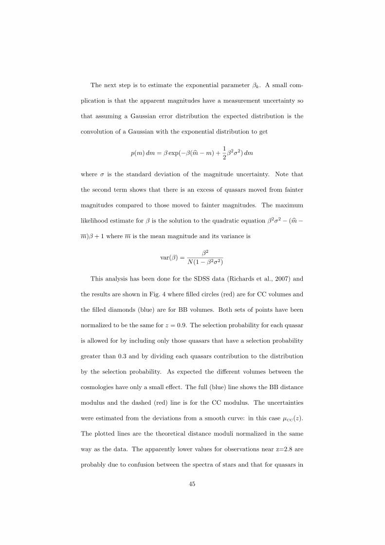
the results are shown in Fig. 4 where filled circles (red) are for CC volumes and

the filled diamonds (blue) are for BB volumes. Both sets of points have been

normalized to be the same for z = 0.9. The selection probability for each quasar

is allowed for by including only those quasars that have a selection probability

greater than 0.3 and by dividing each quasars contribution to the distribution

by the selection probability. As expected the different volumes between the

cosmologies have only a small effect. The full (blue) line shows the BB distance

modulus and the dashed (red) line is for the CC modulus. The uncertainties

were estimated from the deviations from a smooth curve: in this case µCC(z).

The plotted lines are the theoretical distance moduli normalized in the same

way as the data. The apparently lower values for observations near z=2.8 are

probably due to confusion between the spectra of stars and that for quasars in

45

this region which not only produces lower selection probabilities but also makes

their estimates more uncertain. The very clear result is that the quasars are

consistent with CC but they are not consistent with BB without evolution.

Figure 4: The distance modulus of SDSS quasars as a function of redshift. The

diamonds (blue) are for BB and the circles (red) are for CC. The full (blue) line

is the theoretical distance modulus for BB and the dotted (red) line is for CC.

All have been normalized to be the same at z = 0.9.

The conclusion is that CC clearly fits the data whereas BB would require

evolution that cancels the expansion term in its distance modulus.

4.7 Radio Source Counts

The count of the number of radio sources as a function of their flux density

is one of the earliest cosmological tests that arose from the development of

radio astronomy after World War II. Indeed, this test played a pivotal role

46

in the rejection of the steady state cosmology of Bondi, Gold, and Hoyle in

favor of the Big-Bang evolutionary model. In recent years, the study of radio

source counts has declined for several reasons both theoretical and experimental.

An important experimental problem is that many radio sources are double or

complex in structure. Whether or not they are resolved depends on their angular

size and the resolution of the telescope. Since their distance is unknown, the

counts are distorted in a way that cannot be readily determined. The main

theoretical problem in Big-Bang cosmology is that the counts are of a collection

of quite different objects such as galaxies and quasars that can have different

types of evolution. Thus, the radio source counts are not very useful in the study

of these objects. However, in CC, the source number density must be the same

at all places and at all times. Curvature cosmology demands that radio source

counts are consistent with a reasonable luminosity number density distribution

that is independent of redshift. Thus it provides a critical test of CC.

In order to clarify the nature of the radio source count distribution let us

start with a simple Euclidean model. Let the observed flux density of a source at

an observed frequency of ν0 be S(ν0) in units of W m−2 Hz−1 and its luminosity

at the emitted frequency ν be L(ν) in units of W Hz−1. For simplicity, let us

assume that all the sources have the same luminosity and that they have a

volume density of N sources per unit volume. Then using the inverse square

law, the observed number of sources with a flux density greater than S is

n(> S) =4πN

3

(L

4πS

)3/2

.

Thus the number density of observed sources is dn/ds = S−5/2. The importance

of this result is that it is customary to multiply the observed densities by S5/2

so that if the universe had Euclidean geometry the distribution as a function of

47

S would be constant. It has the further advantage in that it greatly reduces the

range of numbers involved. However this practice is not used in this analysis.

For CC the area at a distance r is A(r) = 4πR2 sin2(χ) where r = sin(χ)

and χ = ln(1 + z)/√

3. Note that the actual light travel distance is Rχ . Thus

S(ν0)dν0 =L(ν)dν

4πR2 sin2(χ)(1 + z),

where ν = (1+ z)ν0 and the (1+ z) in the divisor allows for the energy loss due

to curvature redshift. Since the ratio of the differentials (the bandwidth factor)

contributes a factor that cancels the energy loss, the result is

S(ν0) =L((1 + z)ν0)4πR2 sin2(χ)

. (22)

It is convenient to replace the distance variable by the redshift parameter z.

Then the differential volume is

dV (r) =4πR3 sin2(χ)√

3(1 + z)dz.

If the luminosity number density is N(L, (1 + z)ν0) the expected radio-

source-count distribution (allowing for the dS/dL term needed to match the

differentials) is

n(S, ν0) =16π2R5

√3

∫ zm

0

sin4 (χ)1 + z

N (L, (1 + z)ν0) dz,

where zm is the limiting redshift.

A major problem with the observations is the difficulty in knowing the se-

lection criteria. Typically, all sources greater than a chosen flux density are

counted in a defined area. Since the flux density measurements are uncertain

and the number of sources is a strong function of the flux density, it is difficult

to assess a statistically valid cut-off for the survey. In a static cosmology, the

48

change in the distribution due to the change in emitting frequency as a function

of z is an added complication. Thus, an essential test of CC is to show that

there is an intrinsic distribution of radio sources that is identical at all redshifts.

Unfortunately, it is not feasible to obtain a definitive distribution. What will be

done is to show that the observations are consistent with a possible distribution.

Thus the aim of this section is to show that there is a distribution N(L, νe) that

provides a reasonable fit to the observations at all frequencies.

A simple distribution has been found that provides a good first approxima-

tion to the intrinsic distribution. Define the variable x by

x =(

L

L∗

)(ν0(1 + z)1GHz

)β

, (23)

where L∗ and β are constants. The first term is the ratio of the absolute flux

density to a reference value, L∗, and the absolute flux density is obtained from

the measured flux density by using Eq. 22. The second term in Eq. 23 contains

the frequency of emission, ν0(1 + z), and is the only frequency contribution in

this simple model. Then the model for the intrinsic radio-source distribution is

N(L, ν) = Ax−α exp(−γx). (24)

where α, β, γ, and A are constants that are found by fitting the model to the

data listed in Table 9. In order to provide realistic values a value of h=0.7 has

been adopted. The results of fitting this distribution to the data are shown in

Table 10. The χ2 goodness of fit was 4360 for 252 DoF. Because of the poor fit,

the estimate of statistical uncertainties has been omitted.

A plot of the data (references in Table 9) with the flux densities in Jy, and the

results of this model is shown in Fig. 5. For clarity the source density (number

per Gpc3) for each set of points for a given frequency has been multiplied by a

49

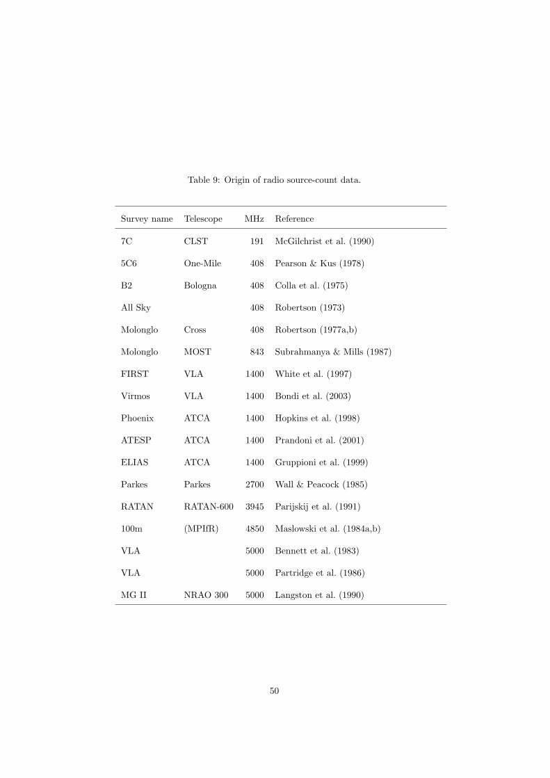
Table 9: Origin of radio source-count data.

Survey name Telescope MHz Reference

7C CLST 191 McGilchrist et al. (1990)

5C6 One-Mile 408 Pearson & Kus (1978)

B2 Bologna 408 Colla et al. (1975)

All Sky 408 Robertson (1973)

Molonglo Cross 408 Robertson (1977a,b)

Molonglo MOST 843 Subrahmanya & Mills (1987)

FIRST VLA 1400 White et al. (1997)

Virmos VLA 1400 Bondi et al. (2003)

Phoenix ATCA 1400 Hopkins et al. (1998)

ATESP ATCA 1400 Prandoni et al. (2001)

ELIAS ATCA 1400 Gruppioni et al. (1999)

Parkes Parkes 2700 Wall & Peacock (1985)

RATAN RATAN-600 3945 Parijskij et al. (1991)

100m (MPIfR) 4850 Maslowski et al. (1984a,b)

VLA 5000 Bennett et al. (1983)

VLA 5000 Partridge et al. (1986)

MG II NRAO 300 5000 Langston et al. (1990)

50

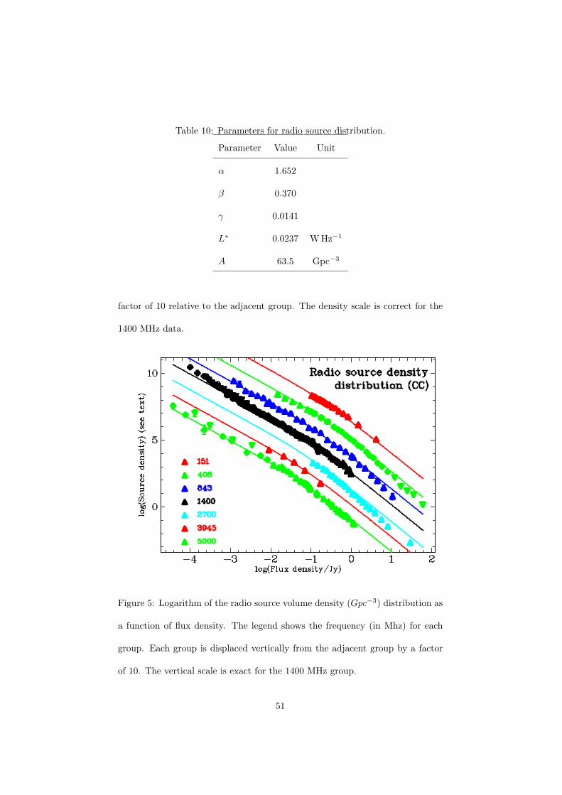
Table 10: Parameters for radio source distribution.

Parameter Value Unit

α 1.652

β 0.370

γ 0.0141

L∗ 0.0237 WHz−1

A 63.5 Gpc−3

factor of 10 relative to the adjacent group. The density scale is correct for the

1400 MHz data.

Figure 5: Logarithm of the radio source volume density (Gpc−3) distribution as

a function of flux density. The legend shows the frequency (in Mhz) for each

group. Each group is displaced vertically from the adjacent group by a factor

of 10. The vertical scale is exact for the 1400 MHz group.

51

Clearly, the model satisfies the basic structure of the distributions but there

is a poor fit at low flux densities, which is probably due to the limitations of

the simple distribution (Eq. 23). It should be emphasized that the only free

parameters are those shown in Table 10. Since the observed densities at low

flux densities are larger than those predicted by the model it suggests that there

may be a second population that is intrinsically fainter that the flux densities

fitted by the model. This analysis shows that a simple distribution of radio

source flux densities can be found that is consistent with the observations. In

Big-Bang cosmology even with the inclusion of evolution there is no model of

radio sources that is as simple as the one described here. Thus, the observations

of the number distribution of radio sources as a function of flux density and

frequency shows that they have no need for luminosity evolution.

4.8 Quasar variability in time

One of the major differences between a tired-light cosmology and an expanding

universe cosmology is that any expanding universe cosmology predicts that time

variations and clocks have the same dependence on redshift as does the frequency

of radiation. Hawkins (2010, 2001, 2003) has analyzed the variability of 800

quasars covering time scales from 50 days to 28 years. His data permitted

the straightforward use of Fourier analysis to measure the time scale of the

variability. He showed that there was no significant change in the time scale

of the variability with increasing redshift. He considered and rejected various

explanations including that the time scales of variations were shorter in bluer

pass bands or that the variations were not intrinsic but were due to intervening

processes such as gravitational micro-lensing. His conclusion was either that

52

the quasars are not at cosmological distances or that the expanding universe

cosmologies are incorrect in this prediction. Curvature cosmology on the other

hand would predict just such results. To summarize, the sparse data on quasar

variability strongly supports no time dilation.

4.9 The Butcher–Oemler effect

If there were evidence of significant change in the universe as a function of red-

shift, it would be a detrimental to any static cosmology. Probably the most

important evidence for this cosmic evolution that appears to be independent

of any cosmological model is the Butcher & Oemler (1978) effect. Although

they had discussed the effect in earlier papers, the definitive paper is Butcher

& Oemler (1984). They observed that the fraction of blue galaxies in galactic

clusters appears to increase with redshift. Clusters allow the study of large num-

bers of galaxies at a common distance and out to large redshifts, which makes

them ideal for studies in evolution. The core regions in a cluster are dominated

by early-type (elliptical and lenticular) galaxies, which have a tight correla-

tion between their colors and magnitudes. We can calculate R30, the projected

cluster-centric radius that contains 30% of the total galaxy population. The

blue fraction, fB , is defined to be the fraction of galaxies within R30 which are

bluer than the color-magnitude relationship for that cluster. At first sight, this

may appear to be a simple test that could be done with apparent magnitudes.

However to compare the ratio for distant clusters with that for nearby ones the

colors must be measured in the rest frame of each cluster, hence the need to use

K-corrections. The major advantage of the Butcher–Oemler effect is that it is

independent of the luminosity-distance relationship that is used. Therefore, to

53

be more precise fB is the fraction that has an absolute magnitude MV , whose

rest frame (B-V) color is at least 0.2 magnitudes bluer than expected. A review

by Pimbblet (2003) summaries the important observations.

In its original form the Butcher–Oemler effect is dependent on the apparent

magnitude cut-off limits. It is essential that selection effects are the same in

the rest frame for each cluster. There are further complications in that the

percentage of blue galaxies may or may not depend on the richness of the cluster

and the effect of contamination from background galaxies. Although Pimbblet

(2003) concluded there was a definite effect, his fig. 1 shows that this conclusion

is open to debate. Since then there have been several attempts to measure

an unambiguous effect. Even though they attempted to duplicate the original

methodology of Butcher & Oemler, de Propris et al. (2003a) found essentially

no effect for K-selected galaxies. Andreon, Lobo & Iovino (2004) examined

three clusters around z=0.7 and did not find clear-cut evidence for the effect.

To quote one of their conclusions: Twenty years after the original intuition

by Butcher & Oemler, we are still in the process of ascertaining the reality of

the Butcher–Oemler effect. The Butcher–Oemler effect remains uncertain, and

therefore does not provide evidence to refute a static cosmology.

5 Conclusion

The major conclusion from this evaluation of Big Bang cosmologies is that all

of the topics covered namely Tolman surface brightness, type 1a supernova,

angular size, gamma ray bursts, galaxy distribution, quasar distribution, radio

source counts, quasar variability in time and the Butcher–Oemler effect are

54

in good agreement with a static universe. Furthermore quantitative estimates

of evolution derived within the BB paradigm are very close to what would be

predicted by BB with a time dilation term of (1+z) removed from the equations.

Acknowledgments

This research has made use of the NASA/IPAC Extragalactic Database (NED)

that is operated by the Jet Propulsion Laboratory, California Institute of Tech-

nology, under contract with the National Aeronautics and Space Administra-

tion. The calculations have used Ubuntu Linux and the graphics have used the

DISLIN plotting library provided by the Max-Plank-Institute in Lindau.

A Analytic Methods

Traditional least squares regression provides two lines, the regression of y on

x and the regression of x on y. In general, these regression lines do not have

reciprocal slopes. If the data includes values for the uncertainties in both coordi-

nates, the traditional minimization of χ2 methods would ignore the uncertainty

in the independent variable. A better solution is obtained by the subroutine

fitexy provided by Press et al. (2007) in their book Numerical Recipes, which

also gives the basic references. This solution uses both sets of uncertainties in

a completely symmetric manner that has a single solution regardless of which

variable is deemed to be the independent. The method for estimating a and b

in y = a + bx is to minimize the χ2 function defined by

χ2 =∑

i

(yi − a − bxi)2

σ2i + b2ε2

i + η2,

55

where σi is the uncertainty in yi, εi is the uncertainty in xi and η is described

below. It is apparent that this equation has the basic symmetry in that if η is

zero then interchanging x and y will give the reciprocal of the slope b. If all the

ε are zero it has an analytic solution otherwise the minimization can be done

numerically.

A problem arises when the χ2 value is significantly different from the number

of degrees of freedom. The case where the value of χ2 is much less than the

number of degrees of freedom is handled by multiplying the uncertainties by

the square root of the ratio of χ2 to the degrees of freedom. If the χ2 is larger

than the number of degrees of freedom the approach used here is to assume

that there is an additional, unknown contribution which is uncorrelated with

the existing uncertainties. This is a common occurrence when the uncertainties

are measurement errors and may be precise but some other factor makes a

significant contribution the scatter of values. the solution is to add a quadratic

term, η2, to the denominator and estimate its value by making the χ2 equal to

the degrees of freedom. The prime advantage of this technique is that it provides

a smooth transition from the situation where the given uncertainties dominate

to the alternative where they are negligible. The main effect is a change in the

relative weights.

References

Andreon, A., Lobo, C. & Iovino, A., (2004). Extending the Butcher-Oemler

effect up to z 0.7. MNRAS, 349, 889.

Astier, A., Guy, J., Regnault, N., Pain, R., Aubourg, E., Balam, D., Basa, S.,

56

Carlberg, R. G., Fbbro, S., Fouchez, D., Hook, I.M., Howell, D. A., Lafoux,

H., Neill, J. D., Palanque-Delabrouille, N., Perrett, K., Pritchet, C.J., Rich,

J., Sullivan, M., Taillet, R., Aldering, G., Antilogus, P., Arsenijevic, V., Bal-

land, C., Baumont, S., Bronder, J., Courtois, H., Ellis, R. S., Filiol, M.,

Gonalves, A. C., Goobar, A., Guide, D., Hardin, D., Lusset, V., Lidman, C.,

McMahon, R., Mouchet, M., Mourao, A., Perlmutter, S., Ripoche, P., Tao,

C. & Walton, N., (2005). SNLS: Measurement of ΩM , ΩΛ and w from the

First Year Data Set. Astronomy and Astrophysics, 207, 1504.

Bennett, C.L., Lawrence, C.R., Hewitt, J.N. & Burke, B.F., (1983). The MIT-

Green Bank (MG) 5 GHz Survey. BAAS., 15, 935.

Blanton, M.R. & Moustakas, J., (2009). Physical Properties and Environments

of Nearby Galaxies. Annual Review of Astronomy and Astrophysics, 47, 159.

Bloom, J.S., Frail, D.A., & Kulkarni, S.R., (2003). Are there more EGRET

Blazars? Astrophysical Journal, 594, 674.

Bondi, M., Ciliegi, P., Zamorani, G., Gregorini, L., Vettolani, G., Parma, P., de

Ruiter, H., Le Fevre, O., Arnaboldi, M., Guzzo, L., Maccagni, D., Scaramella,

R., Adami, C., Bardelli, S., Bolzonella, M., Bottini, D., Cappi, A., Foucaud,

S., Franzetti, P., Garilla, B., Gwyn, S., Ilbert, O., Iovino, A., Le Brun, V.,

Marano, B., Marinoni, C., McCracken, H.J., Menaux, B., Pollo, A., Pozzetti,

L., Radovich, M., Ripepi, V., Rizzo, D., Scodeggio, M., Tresse, L., Zanichelli,

A. & Zucca, E., (2003). The VLA-VIRMOS Deep Field. I. Radio observations

probing the mu Jy source population. Astronomy and Astrophysics, 403, 857.

Borgonovo, L., (1994). Bimodal distribution of the autocorrelation function in

gamma-ray bursts. Astronomy and Astrophysics, 418, 487.

57

Buchalter, A., Helfand, D.J., Becker, R.H. & White, R.L., (1998). Constraining

Omega0 with the Angular Size–Redshift Relation of Double-lobed Quasars in

the FIRST Survey. Astrophysical Journal, 494, 503.

Butcher, H. & Oemler, A. Jr., (1978). The evolution of galaxies in clusters. I -

ISIT photometry of C1 0024+1654 and 3C 295. Astrophysical Journal, 219,

18.

Butcher, H. & Oemler, A. Jr., (1984). The evolution of galaxies in clusters. V

- A study of populations since Z approximately equal to 0.5. Astrophysical

Journal, 285, 426.

Chang, H.-Y, (2001). Fourier Analysis of Gamma-Ray Burst Light Curves:

Searching for a Direct Signature of Cosmological Time Dilation. Astrophysical

Journal, 557, L85.

Chang, H.-Y., Yoon, S.-J. & Choi, C.-S., (2002). A possible use of Fourier Trans-

form analysis method as a distance estimator. Astronomy and Astrophysics,

383, L1.

Colla, G., Fanti, C., Fanti, R., Gioia, C., Lari, C., Lequeux, J., Lucas, R. &

Ulrich, M.H., (1975). Radio and optical data on a complete sample of radio

faint galaxies. Astronomy and Astrophysics Supplement, 20, 1.

Crawford, D.F., (2006). Curvature Cosmology, Boca Ratan, BrownWalker

Press.

Crawford, D.F., (2009). (2nd ed. of CC),

http://www.davidcrawford.bigpondhosting.com.

58

Crawford, D.F., (2009). Observations of type 1a supernovae are consistent with

a static universe. arXiv:0901.4169.

Davis, T. M.; Mortsell, E., Sollerman, J., Becker, A. C., Blondin, S., Challis,

P., Clocchiatti, A., Filippenko, A. V., Foley, R. J., Garnavich, P. M., Jha,

S., Krisciunas, K., Kirshner, R. P., Leibundgut, B., Li, W., Matheson, T.,

Miknaitis, G., Pignata, G., Rest, A., Riess, A. G., Schmidt, B. P., Smith,

R. C., Spyromilio, J., Stubbs, C. W., Suntzeff, N. B., Tonry, J. L., Wood-

Vasey, W. M. & Zenteno, A., (2007). Scrutinizing Exotic Cosmological Models

Using ESSENCE Supernova Data Combined with Other Cosmological Probes.

Astrophysical Journal, 666, 716.

Davis, S.P., Norris, J.P., Kouveliotou, C., Fishman, C., Meegan, C.A. Pasiesas,

W.C., (1994). ”Pulse Width Distributions and Total Counts as Indicators of

Cosmological Time Dilation in Gamma-Ray Bursts” in AIP Conf. Proc. 307,

Gamma-Ray Bursts,ed. G. J. Fishman, J. J. Brainard & K. C. Hurley New

York, AIP, 182.

de Propris, R., Colless, M., Driver, S. P., Couch, W., Peacock, J. A., Baldry,

I. K., Baugh, C. M., Bland-Hawthorn, J., Bridges, T., Cannon, R., Cole, S.,

Collins, C., Cross, N., Dalton, G. B., Efstathiou, G., Ellis, R. S., Frenk, C.

S., Glazebrook, K., Hawkins, E., Jackson, C. Lahav, O., Lewis, I., Lumsden,

S., Maddox, S., Madgwick, D. S., Norberg, P., Percival, W., Peterson, B.,

Sutherland, W. & Tayloer, K., (2003a). The 2dF Galaxy Redshift Survey:

the luminosity function of cluster galaxies. MNRAS, 342, 725.

Disney, M.J., (2000). The Case Against Cosmology. General Relativity and

Gravitation, 32, 1125.

59

Djorgovski, S.G. & Spinrad H., (1981). Toward the application of metric size

function in galactic evolution and cosmology. Astrophysical Journal, 251, 417.

Ellis, G. F. R., (1984). Alternatives to the Big Bang. Annual Review of Astron-

omy and Astrophysics, 22, 157.

Faranoff, B.L. & Riley, J.M., (1974). The morphology of extragalactic radio

sources of high and low luminosity. MNRAS, 167, 31.

Fenimore, E.E. & Bloom J.S., (1995). Determination of Distance from Time

Dilation of Cosmological Gamma-Ray Bursts. Astrophysical Journal, 453,

25.

Goldhaber, G., Groom, D. E., Kim, A., Algering, G., Astier, P., Couley, A.,

Deustua, S. E., Ellis, R., Fabbro, S., Fruchter, A. S., Goobar, A., Hook, I.,

Orwin, M., Kim, M., Knop, R. A., Lidman, C., McMahon, R., Nugent, P. E.,

Pain, R., Panagia, N., Pennypacker, C. R., Perlmutter, S., Ruiz-Lapuente, P.,

Schaefer, B., Walton, N. A. & York, T., (2001). Timescale Stretch Parame-

terization of Type Ia Supernova B-Band Light Curves. Astrophysical Journal,

558, 359.

Goobar, A. & Perlmutter, S., (1995). Feasibility of Measuring the Cosmologi-

cal Constant Lambda and Mass Density Omega Using Type IA Supernovae.

Astrophysical Journal, 450, 14.

Gould, R.J. & Burbidge, G.R., (1963). X-Rays from the Galactic Center, Ex-

ternal Galaxies, and the Intergalactic Medium. Astrophysical Journal, 138,

969.

Gruppioni, C., Cilieg1, P., Rowan-Robinson, M., Cram, L., Hopkins, A., Ce-

60

sarsky, C., Danese, L., Franceschini, A., Genzel, R., Lawrence, A., Lemke, D.,

McMahone, R. G., Miley, G., Oliver, S., Puget, J.-L. & Rocca-Volmerange,

B., (1999). A 1.4-GHz survey of the southern European Large-Area ISO Sur-

vey region. MNRAS, 305, 297.

Gurvits, L.I., Kellermann K.I. & Frey S., (1999). The ”angular size - redshift”

relation for compact radio structures in quasars and radio galaxies. Astronomy

and Astrophysics, 342, 378.

Guth J.E., (1981). Inflationary universe: A possible solution to the horizon and

flatness problems. Phys. Rev. D, 23, 347.

Guy, J., Astier, P., Nobili, S., Regnault, N. & Pain R., (2005). SALT: a spec-

tral adaptive light curve template for type Ia supernovae. Astronomy and

Astrophysics, 443, 781.

Hamuy, M., Phillips, M.M., Schommer, R.A. & Suntzeff, N.B., (1996). The Ab-

solute Luminosities of the Calan/Tololo Type IA Supernovae. Astronomical

J., 112, 2391

Hawkins M.R.S., (2001). Time Dilation and Quasar Variability. Astrophysical

Journal, 553, L97.

Hawkins M.R.S., (2003). Colour changes in quasar light curves. MNRAS, 344,

492.

Hawkins M.R.S., (2010). On time dilation in quasar light curves. MNRAS, 405,

1940.

Hillebrandt, W. & Niemeyer, J.C., (2000). Type IA Supernova Explosion Mod-

els. Annual Review of Astronomy and Astrophysics, 38, 191.

61

Hogg D.W., (1999). Distance measures in cosmology. astro-ph/9905116.

Hogg, D.W., Baldry, I.K., Blanton, M.R. & Eisensteint D.J., 2002. The K cor-

rection. astr-ph/0210394.

Hopkins, A.M., Mobasher, B., Cram, L. & Rowan-Robinson, M., (1998). The

PHOENIX Deep Survey: 1.4-GHz source counts. MNRAS, 296, 839.

Hoyle, F., Burbidge, G. & Narlikar, J.V. (2002). ”A different approach to cos-

mology : from a static universe through the big bang towards reality”, Cam-

bridge Univerity Press.

Joseph, R. (2010). The Infinite Universe vs the Myth of the Big Bang: Red

Shifts, Black Holes,Acceleration, Life. Journal of Cosmology, 6, 1547.

Knop, R. A., Aldering, G., Amanullah, R., Astier, P., Blanc, G., Burns, M.

S., Conley, A., Deustua, S. E., Doi, M., Ellis, R., Fabbro, S., Folatelli, G.,

Fruchter, A. S., Garavini, G., Garmond, S., Garton, K., Gibbons, R., Gold-

haber, G., Goobar, A., Groom, D.E., Hardin, D., Hook, I., Howell, D.A., Kim,

A. G., Lee, B. C., Lidman, C., Mendez, J., Nobili, S., Nugent, P. E., Pain,

R., Panagia, N., Pennypacker, C. R., Perlmutter, S., Quimby, R., Raux, J.,

Regnault, N., Ruiz-Lapuente, P., Sainton, G., Schaefer, B., Schahmabeche,

K., Smith, E., Spadafora, A. L., Stanishev, V., Sullivan, M., Walton, N. A.,

Wang, L., Wood-Vasey, W. M. & Yasuda, N., (2003). New Constraints on Ωλ,

ΩM and w from an Independent Set of 11 High-Redshift Supernovae Observed

with the Hubble Space Telescope. Astrophysical Journal, 598, 102.

Kormendy, J., (1977). Brightness distributions in compact and normal galaxies.

II - Structure parameters of the spheroidal component. Astrophysical Journal,

218, 333.

62

Kowalski, M., Rubin, D., Aldering, G., Agostinho, R. J., Amadon, A., Aman-

ullah, R., Balland, C., Barbary, K., Blanc, G., Challis, P. J., Conley, A.,

Connolly, N. V., Covarrubias, R., Dawson, K. S., Deustua, S. E., Ellis, R.,

Fabbro, S., Fadeyev, V., Fan, X., Farris, B., Folatelli, G., Frye, B. L., Gar-

avini, G., Gates, E. L., Germany, L., Goldhaber, G., Goldman, B., Goobar,

A., Groom, D. E., Haissinski, J., Hardin, D., Hook, I., Kent, S., Kim, A. G.,

Knop, R. A., Lidman, C., Linder, E. V., Mendez, J., Meyers, J., Miller, G.

J., Moniez, M., Mourao, A. M., Newberg, H., Nobili, S., Nugent, P. E., Pain,

R., Perdereau, O., Perlmutter, S., Phillips, M. M., Prasad, V., Quimby, R.,

Regnault, N., Rich, J., Rubenstein, E. P., Ruiz-Lapuente, P., Santos, F. D.,

Schaefer, B. E., Schommer, R. A., Smith, R. C., Soderberg, A. M., Spadafora,

A. L., Strolger, L. -G., Strovink, M., Suntzeff, N. B., Suzuki, N., Thomas, R.

C., Walton, N. A., Wang, L., Wood-Vasey, W. M. & Yun, J. L., (2008). Im-

proved Cosmological Constraints from New, Old, and Combined Supernova

Data Sets. Astrophysical Journal, 686, 749.

Lal, A.K. (2010). Big Bang? A Critical Review. Journal of Cosmology, 6, 1533.

Langston. G.I., Heflin M.B., Conner. S.R., Lehr. J., Carrili C.L. & Burke B.F.,

1990. The second MIT-Green Bank 5 GHz survey. Astrophysical Journal Sup-

plement, 72, 621.

Lee, A., Bloom, E.D. & Petrosian, V., (2000). On the Intrinsic and Cosmological

Signatures in Gamma-Ray Burst Time Profiles: Time Dilation. Astrophysical

Journal, 131, 21.

Lerner, E. J. (1991). The big bang never happened. Random House, New York.

63

Liddle, A.E. & Lyth, D.H., 2000, Cosmological Inflation and Large-Scale Struc-

ture, Cambridge University Press.

Linde, A.D., (1990), Particle Physics and Inflationary Cosmology, Harwood,

New York.

Lopez-Corredoria M., (2010). Angular Size test.on the Expansion of the Uni-

verse. (arXiv 1002.0525v1) International Journal of Modern Physics D, 19,

245.

Lubin, L.M. & Sandage, A., (2001a). The Tolman Surface Brightness Test for

the Reality of the Expansion. II. The Effect of the Point-Spread Function and

Galaxy Ellipticity on the Derived Photometric Parameters. Astronomical J.,

121, 2289.

Lubin, L.M. & Sandage, A., (2001b). The Tolman Surface Brightness Test for

the Reality of the Expansion. III. Hubble Space Telescope Profile and Surface

Brightness Data for Early-Type Galaxies in Three High-Redshift Clusters.

Astronomical J., 122, 1071.

Lubin, L. M. & Sandage, A., (2001c). The Tolman Surface Brightness Test for

the Reality of the Expansion. IV. A Measurement of the Tolman Signal and

the Luminosity Evolution of Early-Type Galaxies. Astronomical J., 122, 1084.

McGilchrist, M.M., Baldwin, J.E., Riley, J.M. Titterington, D.J., Waldram,

E.M. & Warner, P.J., (1990). The 7c Survey of Radio Sources at 151-MHZ -

Two Regions Centred at Ra: 10H28M Dec: 41DEG and Ra: 06H28M Dec:

45DEG. MNRAS, 246, 110.

64

Maslowski, J. Pauliny-Toth, I.I.K., Witzel, A. & Kuhr, H., (1984a). A deep

survey of the 5C2 area at 4850 MHz. Astronomy and Astrophysics, 139, 85.

Maslowski, J., Pauliny-Toth, I.I.K., Witzel, A. & Kuhr H., (1984b). A 4850

MHz survey of a part of the ’GB region’ and the combined counts of sources.

Astronomy and Astrophysics, 141, 376.

Meszaros, P., (2006). Gamma-ray bursts. Rep. Prog. Phys., 2259.

Mitrofanov I.G., Chernenko A.M., Pozanenko A.S., Briggs M.S., Paciesas W.S.,

Fishman G.J., Meegan C.A., Sagdeev R. Z., Chernenko, Anton M.; Poza-

nenko, Alexei S.; Briggs, Michael S.; Paciesas, William S.; Fishman, Gerald

J.; Meegan, Charles A.; Sagdeev & Roald Z., (1996). The Average Intensity

and Spectral Evolution of BATSE Cosmic Gamma-Ray Bursts Astrophysical

Journal, 459,570.

Norris, J.P., (2002). Implications of the Lag-Luminosity Relationship for Unified

Gamma-Ray Burst Paradigms. Astrophysical Journal, 579, 386.

Norris, J.P., Nemiroff, R.J., Scargle, J.D., Kouveliotou, C., Fishman, G.J., Mee-

gan, C.A., Paciesas, W.S. & Bonnell, J.T., (1994). Detection of signature

consistent with cosmological time dilation in gamma-ray bursts. Astrophysi-

cal Journal, 424 540.

Parijskij, Yu. N., Bursov, N.N., Lipovka, N.M., Soboleva, N.S. & Temirova,

A.V., (1991). The RATAN-600 7.6 CM catalog of radio sources from ’Exper-

iment Cold-80’. Astronomy and Astrophysics Supplement, 87, 1.

Partridge, R.B., Hilldrup, K.C. & Ratner M.I., (1986). Radio source counts at

6 centimeters to 0.1 millijanskys. Astrophysical Journal, 308, 46.

65

Peacock, J.A., (1999), Cosmological Physics, Cambridge University Press.

Pearson, T.J. & Kus, A.J., (1978). The 5C 6 and 5C 7 surveys of radio sources.

MNRAS, 182, 273.

Peebles, P.J.E., (1993), Principles of Physical Cosmology, New Jersey, Prince-

ton.

Perlmutter, S., Gabi, S., Goldhaber, G., Goobar, A., Groom, D. E., Hook, I.

M., Kim, A. G., Kim, M. Y., Lee, J. C., Pain, R., Pennypacker, C. R., Small,

I. A., Ellis, R. S., McMahon, R. G., Boyle, B. J., Bunclark, P. S., Carter, D.,

Irwin, M. J., Glazebrook, K., Newberg, H. J. M, Filippenko, A. V.,Matheson,

T., Dopita, M. & Couch, W.J., (1997). Measurements of the Cosmological

Parameters Omega and Lambda from the First Seven Supernovae at Z ¿=

0.35. Astrophysical Journal, 483, 565.

Perlmutter, S., Aldering, G., Goldhaber, G., Knop, R.A., Nugent, P., Cas-

tro, P.G., Deustua, S., Fabbro, S., Goobar A., Groom, D. E., Hook, I. M.,

Kim, A. G., Kim, M, Y., Lee, J. C, Nunes, N. J., Pain, R., Pennypacker,

C. R., Quimby, R., Lidman, C., Ellis, R. S., Irwin, M., McMahon, R. G.,

Ruiz-Lapuente, P., Walton, N., Shaefer, B., Boyle, B. J., Filippenko, A. V.,

Matheson, T., Fruchter, A. S., Panagia, N., Newberg, H. J. M. & Couch,

W. J., (1999). Measurements of Omega and Lambda from 42 High-Redshift

Supernovae. Astrophysical Journal, 517, 565.

Perlmutter, S. & Schmidt, B.P. (2003). ” Measuring Cosmology with Super-

novae” in Supernovae, Gamma Ray Bursts, K. Weiler, ed. (Springer: New

York).

66

Petrosian, V. (1976). Surface brightness and evolution of galaxies. Astrophysical

Journal, 209, 1.

Phillips, M.M., (1993). The absolute magnitudes of Type IA supernovae. As-

trophysical Journal, 413, L105.

Pimbblet, K.A. (2003). At the Vigintennial of the Butcher-Oemler Effect. Pub.

Astr. Soc. Aust., 20, 294.

Piran, T., (2004). The physics of gamma-ray bursts. Rev. Mod. Phys, 76, 1143.

Postman, M. & Lauer, T.R., (1995). Brightest cluster galaxies as standard can-

dles. Astrophysical Journal, 440, 28.

Pound, R.V. & Snyder, J.L., (1965). Effect of Gravity on Gamma Radiation.

Phys. Rev. B, 140, 788.

Prandoni, I., Gregorini, L., Parma, P., de Ruiter, H.R., Vettolani, G., Wieringa,

M.H., Ekers R. D., (2001). The ATESP radio survey. III. Source counts.

Astronomy and Astrophysics, 365, 392

Press, W.H., Teukolsky, A.A., Vetterling, W.T., Flannery & B.P., (2007). Nu-

merical Recipes in Fortran 77, Cambridge University Press.

Richards, G. T., Strauss, M. A., Fan,X., Hall, P. B., Jester, S., Schneider, D. P.,

Vanden Berk, D. E., Stoughton, C., Anderson, S. F., Brunner, R. J., Gray, J.,

Gunn, J. E., Ivezic,Z., Kirkland, M. K., Knapp, G. R., Loveday, J., Meiksin,

A., Pope, A., Szalay, A. S., Thakar, A. R., Yanny, B., York, D. G., Barentine,

J. C., Brewington, H. J., Brinkmann, J., Fukugita, M., Harvanek, M.l, Kent,

S. M., Kleinman, S. J., Krzesin’ski, J., Long, D. C., Lupton, R. H., Nash, T.,

Neilsen, E. H., Jr., Nitta, A., Schlegel, D. J. & Snedden, S. A., (2007). The

67

Sloan Digital Sky Survey Quasar Survey: Quasar Luminosity Function from

Data Release 3. Astronomical J., 131, 2766.

Richardson, D., Branch, D., Casebeer, D., Millard, J., Thomas, R.C. & Baron,

E., (2002). Spectroscopic Target Selection in the Sloan Digital Sky Survey:

The Quasar Sample Astron. J. 123, 2945.

Riess, A. G., Strolger, L. -G., Tonry, J., Casertano, S., Fergusen, H. C.,

Mobasher, B., Challis, P., Filippenko, A. V., Jha, S., Li, W., Chornock,

R., Kirshner, R. P., Leibundgut, B., Dickinson, M., Livio, M., Giavalisco,

M., Steidel, C. C., Benitez, N. & Tsvetanov, Z., (2004). Type Ia Supernova

Discoveries at z ¿ 1 from the Hubble Space Telescope: Evidence for Past De-

celeration and Constraints on Dark Energy Evolution. Astrophysical Journal,

607, 665.

Riess, A. G., Li, W., Stetson, P. B., Filippenko, A. V., Jha, S., Kirshner, R. P.,

Challis, P. M., Garnavitch, P. M. & Chornock, R., (2005). Cepheid Calibra-

tions from the Hubble Space Telescope of the Luminosity of Two Recent Type

Ia Supernovae and a Redetermination of the Hubble Constant. Astrophysical

Journal, 627, 579.

Robertson, J.G., (1973). An all-sky catalogue of strong radio sources at 408

MHz. Aust. J. Phys., 26, 403.

Robertson, J.G., (1977a). The Molonglo deep sky survey of radio sources. I -

Declination zone -20 deg. Aust. J. Phys., 30, 209.

Robertson, J.G., (1977b). The Molonglo deep sky survey of radio sources. II.

Declination zone -62. Aust. J. Phys., 30, 231.

68

Rowan-Robertson, M., (1985). The Cosmological Distance Ladder, New York,

W. H. Freeman & Co.

Sandage, A., Lubin, L.M., 2001. The Tolman Surface Brightness Test for the

Reality of the Expansion. I. Calibration of the Necessary Local Parameters.

Astronomical J., 121, 2271.

Sandage, A., Perelmuter, J.-M., (1990). The surface brightness test for the ex-

pansion of the universe. I - Properties of Petrosian metric diameters. Astro-

physical Journal, 350, 481.

Sandage, A., (2010). The Tolman Surface Brightness Test for the Reality of the

Expansion. V. Provenance of the Test and a New Representation of the Data

for Three Remote Hubble Space Telescope Galaxy Clusters. Astronomical J.,

139,728.

Schneider, D. P., Hall, P. B., Richards, G. T., Vanden Berk, D. E., Anderson, S.

F., Fan, X., Jester, S., Stoughton, C., Strauss, M. A., SubbaRao, M., Brandt,

W. N., Gunn, J. E., Yanny, B., Bahcall, N. A., Barentine, J. C., Blanton, M.

R., Boroski, W. N., Brewington, H. J, Brinkmann, J., Brunner, R., Csabai, I.,

Doi, M., Eisenstein, D. J., Friemann, J. A., Fukugita, M., Gray, J., Harvanek,

M., Heckman, T. M., Ivezic,Z., Kent, S., Kleinman, S. J., Knapp, G. R., Kron,

R. G., Krzesinski, J., Long, D. C., Loveday, J., Lupton, R. H., Margon, B.,

Munn, J. A., Neilsen, E. H., Newberg, H. J., Newman, P. R., Nichol, R. C.,

Nitta, A., Pier, J.R., Rockosi, C. M., Saxe, D. H., Schlegel, D. J., Snedden, S.

A., Szalay, A. S., Thaker, A. R., Uomoto, A. & York, D. G., (2005). The Sloan

Digital Sky Survey Quasar Catalog. III. Third Data Release. Astronomical

J., 130, 367.

69

Schneider, D. P., Hall, P. B., Richards, G. T., Strauss, M. A., Vanden Berk, D.

E., Anderson, S. F., Brandt, W. N., Fan, X., Jester, S., Gray, J., Gunn, J.

E., SubbaRao, M. U., Thakar, A. R., Stoughton, C., Szalay, A. S., Yanny, B.,

York, D. G., Bahcall, N. A., Barentine, J., Blanton, M. R., Brewington, H.,

Brinkmann, J.,Brunner, R. J., Castander, F. J., Csabai, I., Frieman, J. A.,

Fukugita, M., Harvanek, M., Hogg, D. W., Ivezic, Z., Kent, S. M., Kleinman,

S. J., Knapp, G. R., Kron, R. G., Krzesin’ski, J., Long, D.l C., Lupton, R.

H., Nitta, A., Pier, J. R., Saxe, D. H., Shen, Y., Snedden, S. A., Weinberg,

D. H. & Wu, J., (2007). The Sloan Digital Sky Survey Quasar Catalog. IV.

Fifth Data Release. Astrophysical Journal, 134, 102.

Steinhardt, P.J. & Caldwell, R.R., (1998), Cosmic Microwave Background &

Large Scale Structure of the Universe, Astr. Soc. Pacif. Conf. Ser. 151, 13.

Struck, C., (1999). Galaxy collisions. Phys. Rev. 321,1.

Strolger, L. -G., Riess, A. G., Dahlen, T., Livio, M., Panagia, N., Challis, P.,

Tonry, J. L., Filippenko, A. V., Chornock, R., Fergusen, H., Koekemoer,

A., Mobasher, B., Dickinson, M., Giavalisco, M., Casertano, S., Hook, R.,

Blondin, S., Leibundgut, B., Nonino, M., Rosati, P., Spinrad, H., Steidel,

C.C., Stern, D., Garnavich, P. M., Matheson, T., Grogin, N., Hornschemeir,

A., Kretchmer, C., Laidler, V. G., Lee, K., Lucas, R., de Mello, D., Moustakas,

L. A., Ravindranath, S., Richardson, M. & Taylor, E., (2004). The Hubble

Higher z Supernova Search: Supernovae to z 1.6 and Constraints on Type

Ia Progenitor Models. Astrophysical Journal, 613, 200.

Subrahmanya, C.R. & Mills B.Y., (1987). Molonglo Deep Survey at 843 MHZ.

IAU Symposium, 124, 569.

70

Tolman, R.C., (1934), Relativity, Thermodynamics and Cosmology, Oxford Uni-

versity Press.

Turner, M.S., (1999). ”Dark Matter and Dark Energy in the Universe” in The

Third Stromlo Symposium: The Galactic Halo, Gibson, B. K., Axelrod, T.

S. & Putman, M. E. (eds), Astr. Soc. Pacific Conf. Ser. 165, 431.

Van Flandern, T.C. (2002) The Top 30 Problems with the Big Bang. Meta

Research Bulletin, 11, 6.

Wall, J.V. & Peacock, J.A., (1985). Bright extragalactic radio sources at 2.7

GHz. III - The all-sky catalogue. MNRAS, 216, 173.

White, R.L., Becker, R.H., Helfand, D.J. & Gregg, M.G., (1997). A Catalog of

1.4 GHz Radio Sources from the FIRST Survey. Astrophysical Journal, 475,

479.

Wolf, C., Meisenheimer, K., Rix, H.-W., Borch, A., Dye, S. & Kleinheinrich M.,

(2003). The COMBO-17 survey: Evolution of the galaxy luminosity function

from 25 000 galaxies with 0.2¡ z ¡1.2. Astronomy and Astrophysics, 401, 73.

Wolf, C., Meidenheimer, K., Kleinheinrich, M., Borch, A., Dye, S., Gray, M.,

Wisotski, L., Bell, E. F., Rix, H. -W., Cimatti, A., Hasinger, G. & Szokoly,

G., (2004). A catalogue of the Chandra Deep Field South with multi-colour

classification and photometric redshifts from COMBO-17. Astronomy and

Astrophysics, 421, 913.

Wood-Vasey, W. M.,; Friedman, A. S., Bloom, J. S., Hicken, M., Modjaz, M.,

Kirshner, R. P., Starr, D. L., Blake, C. H., Falco, E. E., Szentgyorgyi, A.

H., Challis, P., Blondin, S. & Rest, A., (2008). Type Ia Supernovae Are

71

Good Standard Candles in the Near Infrared: Evidence from PAIRITEL.

Astrophysical Journal, 689, 377.

Zhang, B., 2007. Gamma-Ray Bursts in the Swift Era. Chin. J. Astron. Astro-

phys., 7, 1.

Zel’dovich, Ya.B., (1963). Special Issue: the Theory of the Expanding Universe

as Originated by a. a. Fridman. Usp. Fiz. Nauk., 80, 357, (1964, Sov. Phys.-

Uspekhi. 6, 475).

Zwicky, F. 1937. On the Masses of Nebulae and of Clusters of Nebulae. Astro-

physical Journal, 86, 217.

72