Proceedings of Indian Geotechnical Conference December 13-15, 2012, Delhi (Paper No.C301.)

GPR SURVEY FOR UTILITY MAPPING AT TWO STATIONS OF HYDERABAD METRO B. Uday Kumar, Post Graduate student, Earthquake Engineering Research Centre IIIT Hyderabad. Akhila Manne, Research student, Earthquake Engineering Research Centre, IIIT Hyderabad. D. Neelima Satyam, Assistant professor, Earthquake Engineering Research Centre, IIIT Hyderabad Email: neelima.satyam@iiit.ac.in

ABSTRACT: Ground Penetration Radar (GPR) has been used to locate the soil characteristics, water table depth, depth of bedrock, buried utilities and cavities below the ground surface. GPR works by sending a tiny pulse of energy into a material and recording the strength and the time required for the return of any reflected signal. A series of pulses over a single area make up what is called a scan. Reflections are produced whenever the energy pulse enters into a material with different electrical conduction properties (dielectric permittivity) from the material it left. The strength, or amplitude, of the reflection is determined by the contrast in the dielectric constants of the two materials. This means that a pulse which moves from dry sand to wet sand will produce a very strong, brilliantly visible reflection, while one moving from dry sand to limestone will produce very weak reflections. Materials with a high dielectric are very conductive. Materials with a high dielectric are very conductive and thus attenuate the signal rapidly. Water saturation dramatically raises the dielectric of a material, so a survey area should be carefully inspected for signs of water penetration. Radar surveys should never be conducted through standing water, no matter how shallow. Depth penetration through a material with a high dielectric will not be very good. At Habsiguda and NGRI stations the GPR survey has been carried out in an area of 130m x 20m for identifying the utility and other service lines. Excavation was also made to check the efficiency of the survey carried out. Keywords: GPR, Utility Survey, Dielectric Permittivity, RADAN INTRODUCTION Prevailing records of the utilities are usually inaccurate and require excavations to confirm while taking up extensive projects like construction of Metro transport system. Even maintenance and upgrading of the utility networks is challenging with such data. Excavations especially that of roads are exhaustive and require ample time as it may result in disruption of traffic and cause accidents. Such problems resulted in over 120,000 utility strikes nationwide in 2007 [1]. Also, huge water supply networks have about 20% of losses caused by pipe leakage [2]. Supporting factors for the need of a rapid exploration technique are: the age and density of the infrastructure systems; utilities that are owned by multiple private sector companies or public agencies; a lack of ‘as built’ drawings and historical maps; undocumented modifications; poor record keeping; and the lack of a single entity responsible for accurate mapping and record keeping [3]. Surveys using sensors such as Ground Penetrating Radar (GPR) can be conducted to alleviate the extent and duration of excavation and benefitting health and safety. Ground penetrating radar (GPR) is a novel geophysical technique. GPR is quite accurate when a quality level C (ASCE 38-02) data is required. The last decade has seen major advances and the history of GPR is intertwined with the diverse applications of the technique [4]. It has the most extensive applications compared to any other technique and limitations too. GPR has been used successfully in a variety of applications such as for highways to identify pavement

thickness, asphalt density, moisture content of base materials, locating anomalies, rutting etc. In case of investigation of natural geologic materials and other construction works. Properties of EM waves explicitly show the possibility to detect pipes of different materials. Differences between reflected waves would be only in amplitude values (reflection strength) [5, 6]. Beside several another modern methods GPRs have a significant role in the process of quick and efficient detection of pipe leakage, especially in pipes with small diameter. Identification of pipe leakage is possible by detection of cavities created by leaking fluids, or analyzing changes in soil structure caused by moisture (change of dielectric permittivity ε) [2]. Suitability of the radar depends on site conditions. It works best for near surface, dry soil conditions where the dielectric contrast is greatest, and conversely does not work well in wet, clayey soil conditions where the dielectric contrast is negligible. In this paper, GPR survey has been employed for utility mapping for excavation, required for the construction of metro stations at two locations, Habsiguda and NGRI. THEORY AND BACKGROUND GPR consists of a control unit, antenna and power supply. The control unit has a hard disk, built-in computer and mechanism to trigger the pulse of radar energy (electromagnetic waves) into ground in shape of a cone. The control software allows for the processing of data implicitly

Uday Kumar B,Akhila Manne & ,D.Neelima Satyam

in the field. The antenna amplifies the received signals and transmits them into the ground. Antenna frequency is one major factor in depth penetration. The higher the frequency of the antenna, the shallower into the ground it will penetrate. Antenna choice is one of the most important factors in survey design. Table 1 shows antenna frequency, approximate depth penetration and appropriate application. Table 1 Application of GPR for different Antenna Frequency

GPR works by imparting electromagnetic waves into the ground, and those reflected back towards the surfaces are received by the antenna. Time taken for reflection and the strength of returned signal accounts for the working of GPR. Strength of the reflected energy pulse travelling form one medium to other depends on the difference in dielectric constants and conductivities of the materials. A pulse which moves from dry sand (dielectric of 5) to wet sand (dielectric of 30) will produce a very strong reflection, while moving from dry sand (5) to limestone (7) will produce a relatively weak reflection [5]. Attenuation or amplification of a material depends on the material properties and signal strength. Dielectric constant is is a major parameter in GPR study. Materials with high dielectric constant slow the radar wave penetration and those with high conductivity attenuate the signal. Care has to be taken to identify any water penetration in the survey area as water saturation content of the material affects the dielectric of the material. Metals reflect the signals and hence cannot be detected by GPR. Due to conical emission of energy from the control unit, travel time for energy at the leading edge of cone is longer than for that directly beneath the antenna. Any target is represented by an inverted ‘U’ in the recorded trace. When antenna crosses at a sharp angle above the pipeline axis, the hyperbola has a totally different shape, which is no longer hyperbolic. In an extreme case, when the antenna trajectory is along the pipeline axis, the hyperbola is distorted into a straight line [7]. Detection of pipe materials (non-metal pipe) is possible by measuring differences between reflected waves (reflection strength) [7].

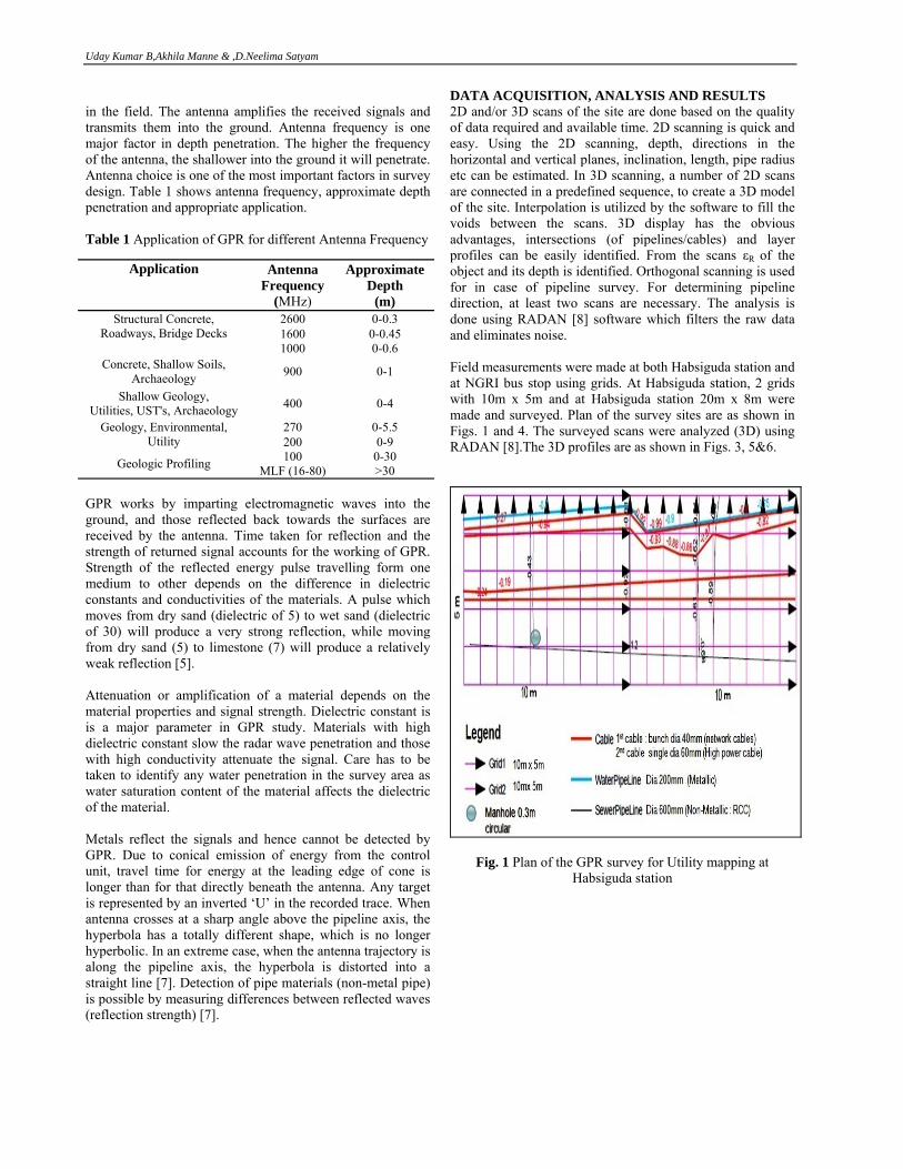
DATA ACQUISITION, ANALYSIS AND RESULTS 2D and/or 3D scans of the site are done based on the quality of data required and available time. 2D scanning is quick and easy. Using the 2D scanning, depth, directions in the horizontal and vertical planes, inclination, length, pipe radius etc can be estimated. In 3D scanning, a number of 2D scans are connected in a predefined sequence, to create a 3D model of the site. Interpolation is utilized by the software to fill the voids between the scans. 3D display has the obvious advantages, intersections (of pipelines/cables) and layer profiles can be easily identified. From the scans εR of the object and its depth is identified. Orthogonal scanning is used for in case of pipeline survey. For determining pipeline direction, at least two scans are necessary. The analysis is done using RADAN [8] software which filters the raw data and eliminates noise. Field measurements were made at both Habsiguda station and at NGRI bus stop using grids. At Habsiguda station, 2 grids with 10m x 5m and at Habsiguda station 20m x 8m were made and surveyed. Plan of the survey sites are as shown in Figs. 1 and 4. The surveyed scans were analyzed (3D) using RADAN [8].The 3D profiles are as shown in Figs. 3, 5&6.

Fig. 1 Plan of the GPR survey for Utility mapping at Habsiguda station

Application Antenna Frequency

(MHz)

Approximate Depth

(m) Structural Concrete,

Roadways, Bridge Decks

2600 0-0.3 1600 0-0.45 1000 0-0.6

Concrete, Shallow Soils, Archaeology 900 0-1

Shallow Geology, Utilities, UST's, Archaeology 400 0-4

Geology, Environmental, Utility

270 0-5.5 200 0-9

Geologic Profiling 100 0-30 MLF (16-80) >30

GPR Survey For Utility Mapping At Two Stations Of Hyderabad Metro

Fig. 2 Free Orbit View at Habsiguda station (sectional) Inferences from Habsiguda survey Two sets of cables (red colored) one in bunch (40mm dia) assumed to be network cables, and other running as single cable (60mm dia) high power cable (as shown in Figs. 2 & 3) are identified from the scans. One water pipe line, metallic of 200 mm dia was detected at 0.7m depth. Sewer pipeline (non-metallic) of 600 mm dia was detected with depths mentioned as in Fig. 6.

Fig. 3 3D Sectional View of utilities at Habsiguda station

Fig. 4 Plan of the Utility survey at NGRI bus stop

Fig. 5 3D sectional view of utilities at NGRI bus stop

Uday Kumar B,Akhila Manne & ,D.Neelima Satyam

Fig. 6 3D view of utilities at NGRI bus stop Manhole invert levels were detected approximately at 2.2 m below GL since the surveyed strata was highly saturated due to rain causing high noise levels. Rain water collection chamber was also identified. Inferences from NGRI bus stop survey At NGRI two water pipe lines of 100 mm were identified in the analysis at depths of 1.36 and 0.91 m below the ground surface. Electrical cable is located at a depth of 1.04 m from ground surface and at a distance of 2.2 m from reference line AD (in between two water lines shown, Fig. 4). Two optical fiber cables at a depth of 0.82 and 0.75 m respectively with a lateral difference of 0.75 m between two cables are observed in the analysis. Three cables were detected in transverse direction at depths of 0.99m, 1.02m and 0.99 m respectively. On excavating the area at five places some minor discrepancy was observed in the results of GPR survey conducted. Although, there is some error of judgment, the scans could be well explained through the excavations. The interpretation made through GPR survey vis a vis observations through pit photographs are as follows. The survey carried out at NGRI bus stop site was up to 55% accurate. One water pipe line was observed going through center of the road and was correctly identified through GPR survey as well. The electrical cable observed in the excavation has been mapped correctly through the survey. The purple colored cables in the longitudinal axis were also detected in the zone of excavation. The purple color cables in the transverse direction and dead cables shown at shallow depths in green color were not detected properly because of presence of loose

soil formations and embedded boulder below the ground. In one cross section line soil cavity was observed (soil loss) which has been misinterpreted as non metallic utility. CONCLUSIONS Utility mapping survey is very important in knowing the all kinds of utility lines for control of underground infrastructure systems. Classic mapping technologies (excavation, old maps) cannot be employed always. For such purpose GPR serves best. GPR is a high-speed, continuous, nondestructive field test and has variety of applications. Though GPR demands expertise to interpret the scans, it is a rapid technique for investigation of utilities. It works by transmitting electromagnetic waves through the survey area and recording the reflected waves and time. Based on the dielectric permittivity the non-metallic materials can be identified and through the analysis, the 2D/3D profile of the surveyed area can be generated. In this paper, two locations in Hyderabad have been surveyed for the purpose of the construction of Metro rail stations. A 3D analysis has been done with the scans generated in the field. The scans were collected orderly by sketching a grid. To verify the results test pits have been excavated. Correlation between GPR interpreted features and utilities observed in the test pit were good with respect to utility location and orientation. REFERENCES 1. DIRT Report (2007), Common Ground Alliance,

www.commongroundalliance.com, 2008. 2. Osama, H., (1998),GPR for detection of leaks in buried

plastic water distribution pipes,7th International Conference on GPR, 27-30 May, Lawrence, Cansas, USA.

3. Mooney, J.P.,Jr., Ciampa, J.D., Young, G.N., Kressner, A.R., Carbonara, J. (2010),GPR Mapping to Avoid Utility Conflicts Priorto Construction of the M-29 Transmission Line ,J. IEEE.

4. Annan A.P., (2002),GPR—History, Trends, and Future, J. Developments Subsurface Sensing Technologies and Applications, Plenum Publishing corporation, Vol. 3, No. 4, October .

5. What is GPR, Geophysical Survey Systems, Inc., www.geophysical.com/WhatisGPR, 2006.

6. Al-Nuaimy, W., Shihab,S., and Eriksen, A., (2004), Data fusion for accurate characterisation of buried cylindrical objects using GPR, 10th International Conference on GPR, 21-24 June, Delft, The Netherlands.

7. Paniagua, J., (2004), Test site for the analysis of subsoil GPR propagation, 10th International Conference on GPR, 21-24 June, Delft, The Netherlands.

8. GSSI, (2006), RADAN 6 User Manual, North Salem, USA.

Proceedings of Indian Geotechnical Conference December 13-15,2012, Delhi (Paper No.C304)

STUDY ON ADVANCED TECHNIQUES USED FOR INSTRUMENTATION AND MONITORING OF RAILWAY TRACK FORMATIONS

L.S. Sowmiya, Research Scholar, Civil Engineering Department, IIT Delhi, sowmiya_lazarus@yahoo.co.in J.T. Shahu, Associate Professor, Civil Engineering Department, IIT Delhi, shahu@civil.iitd.ac.in ABSTRACT: Railways form an important part of the transportation infrastructure of a country and plays an important role in sustaining a healthy economy. Instrumentation is very much useful on the sites where the subgrade failures like mud pumping, excessive settlement and shear failure etc have been experienced. This study includes the available advanced techniques used in the field of instrumentation in railway formations. These field instrumentations have been installed in the problematic sites provide valuable in-situ factors causing mud pumping and the other failures. In general, commercially available sensors such as piezometers, accelerometers, strain gauges and displacement sensors are used in the track monitoring system. To record the maximum values of pressure transmitted from the sleeper through the ballast and of tie reaction, pressure cells and load cells connected directly to the data logger. Remote monitoring system with advanced techniques is used in the developed countries to control the instrumentation sites and collect the in-situ data’s in any time. These different techniques of track monitoring systems can help to maintain the safety of railroad tracks by monitoring settlement, pressure, toe movement, heaving, etc. INTRODUCTION The railway track consists of the man-made superstructure (rail, ties, ballast and sub-ballast) overlying the in-situ ground (subgrade). The performance and serviceability of the superstructure is governed by its ability to provide smooth train rides and inability to do so results in the track maintenance. The performance of the railway track can be compromised by deterioration in the track superstructure (e.g. ballast degradation, bending in rails) and problematic subgrade. The aim of this study is to gain knowledge in the application of monitoring system at a railway site experiencing with problematic subgrade. Problematic subgrade can arise from a variety of mechanisms – mud pumping, progressive shear failure, excessive subgrade deformation etc. Problematic subgrade result in poor track conditions are viewed as a serious safety issue and tracks with historically poor performance are frequently monitored using track alignment-detection vehicles. Li (2000) investigated the track performance prior to and after installation of Hot-Mix-Asphalt (HMA) subgrade improvements using pressure cells and Linear-Variable-Displacement-Transducers (LVDT). Konrad et al. (2007) installed piezometers and wire potentiometers at Canadian National site to measure the settlement. Wong et al. (2006) installed vibrating-wire piezometers for a Canadian Pacific Railway site overlying one to three meters of peat. The site undergoes excessive settlement and form piping holes under repeated heavy axle loads. Indraratna et al. (2010) the track was constructed between two turnouts at Bulli along the New South Coast, Australia. The total length of the instrumented track section was 60 m and was divided into four sections, each of 15 m length. In advanced stage the remote monitoring system was used to record the data’s without man handling. Collecting and analyzing of data’s were easy and time saving also. Aw et al. (2003) gives the report of low cost monitoring system

used in USA for research purpose. This paper gives the summary of instrumentation and monitoring system used in the railway tracks over the world and the simplest method of instrumentation layout for the Indian railway system. The instrumentation included settlement pegs, displacement transducers, and pressure cells and data collection devices etc. INSTRUMENTATION IN RAILWAY TRACK A summary of the instrumentation that can be used for field measurement in railway tracks in the sub soil, blanket/subgrade soil and Ballast is given in Table 1.

Table 1 Summary of Instrumentations used in Railway Track Layers

Property to Measure Instrument to be UsedPore Pressure Pore Pressure Transducers /

PiezometersSettlement Settlement gauges /

settlement pegsHeaving of Ground Soil Heave/Settlement GaugeToe Movement InclinometerPressure Pressure CellSlope Movement InclinometerTie Reaction Load Cell

DETAILS OF INSTRUMENTS Pore Pressure Transducer / Piezometer Typical applications of pore pressure transducer / piezometer are monitoring pore water pressures to evaluate slope stability, monitoring dewatering systems used for excavations and monitoring ground improvement systems, such as vertical drains and sand drains. The other applications of piezometers are like, to check the performance of earth fill dams and embankments and to check containment systems at landfills and tailings dams. Figure 1 (a) shows that the typical pore pressure transducers used in the field.

L.S. Sowmiya, J.T. Shahu

Soil settlement Gauge / Soil heave Gauge / Soil Extensometer

Settlement gauges Settlement gauges can be used to monitor settlement or heave at discrete locations in soil. Settlement gauges are often installed to measure the deformation of the foundation or embankment or to monitor the movement of existing structures that are located adjacent to the area of construction. Fig. 1 (b) shows a typical soil settlement gauge (SSG). Typical applications of settlement gauge include monitoring settlement or heave in embankments and embankment foundations. The other applications are monitoring subsidence due to tunneling and mining, monitoring consolidation under storage tanks, monitoring settlement due to dewatering or preloading and monitoring settlement in fills.

Soil Extensometers Soil Extensometers monitor lateral and longitudinal deformation of soil and different types of embankments. A typical Vibrating Wire Soil Extensometer is shown in Fig 1 (c). The instrument consists of a vibrating wire displacement sensor encased in a sealed body. The body contains a telescopic outer PVC pipe fitted with two flanges and an inner stainless steel rod.

Pressure Cells A pressure cell measures the total stress (= sum of the effective stress and the pore-water pressure). The pressure cell can be manufactured from two circular plates of stainless steel. The edges of the plates are welded together to form a sealed cavity that is filled with fluid (Fig. 1 (d)). A pressure sensor is then attached to the top plate and the pressure cell is connected to a data logger. Typical applications include: determining the distribution, magnitude, and direction of total stresses in an embankment. Pressure cells also used for estimating the overburden pressure acting on foundation, measuring contact pressures in abutments and foundations.

Inclinometer The horizontal movement preceding or during the movement of slopes can be investigated by successive surveys of the

shape and passion of flexible vertical casing installed in the ground. The surveys are performed by lowering a probe into the flexible vertical casing. The inclinometer probe is capable of measuring its deviation from the vertical. Fig. 1 (e) shows a sketch of the inclinometer probe in the casing and the calculations used to obtain the lateral deformation. Typical applications of vertical inclinometers include: (i) monitoring slopes and landslides to detect zones of movement and establish whether movement is constant, accelerating, or responding to remedial measures. (ii) Monitoring diaphragm walls and sheet piles to check that deflections are within design limits; that struts and anchors are performing as expected; and the adjacent buildings are not affected by ground movements. (iii) Monitoring dams, dam abutments, and upstream slopes for movement during and after impoundment. (iv) Monitoring the effects of tunneling operations to ensure that adjacent structures are not damaged by ground movements. Typical applications of horizontal inclinometers include: (i) providing settlement profiles of embankments, foundations, and other structures. (ii) Monitoring deformation of the concrete face of a dam. LAYOUT OF INSTRUMENTATIONS USED IN RAILWAY TRACK A summary of possible instrumentations used for a railway track in the subsoil, blanket/subgrade soil and ballast is already given in Table 1. A data logger of dynamic variety is required to store the measured data. The detailed layout of possible instrumentation used in the Indian railway track condition is shown in Fig. 2. Once all the installations are over then the data collection process may start. The settlement pegs will be surveyed immediately after installation and again after 2 days, then at weekly intervals for 3 weeks, monthly intervals for the next 3 months, 3-month intervals for the next 9 months, and a final survey after 24 months. The measurements may be carried out using simple survey techniques recording the change in the reduced level of the surface of each layer with time. To record the maximum values of tie reaction and the pressure transmitted from the sleeper through the ballast, load cells and pressure cells may be connected directly to the data logger and triggering may be carried out manually for each train. Figure

Fig.1 Instrumentations used in the Railway Track (a) Pore Pressure Transducer, (b) Settlement Gauge, (c) Soil Extensometer, (d) Pressure Cells, (e) Inclinometer

(a) (b) (c) (d) (e)

Study on Advanced Techniques used for Instrumentation and Monitoring of Railway Track Formation

2 (a) shows the plan view of the instrumentation layout. The layout was divided into three control station.

Fig. 2 Layout of Possible Instrumentation Used in Indian Railway Track Condition

Fig. 2 (a) Plan View of Instrumentation Layout

Fig. 2 (b) Section A-A

Fig. 2 (c) Section B-B

Fig. 2 (d) Section C-C

L.S. Sowmiya, J.T. Shahu

These control stations will help to compare the recorded readings in transverse and vertical directions. Manual recording will be carried out throughout the duration of monitoring of the type of passing train (freight or passenger), number and types of cars in the train, nominal car load/wheel load, and the speed of train.

REMOTE (WIRELESS) MONITORING SYSTEM Remote or wireless monitoring system is the advanced technique used in the field of monitoring. Railroad operators generally maintain two different forms of monitoring program. In the regular track degradation detection, mobile instrumentation units are favored over stationary monitoring systems. Mobile instrumentation units often consist of sensors (e.g. inertia systems or Ground Penetrating Radar (GPR)) attached to track vehicles. Ground Penetrating Radar (GPR) is used for ballast degradation detection. Mobile instrumentation units are, however, not suitable for long term point based monitoring, especially at problematic remote locations. Figure 3 shows the schematic diagram of the major components of wireless monitoring system. Data collected from the sensor mesh are streamed to the base station, which are then transmitted through satellite communication and back to the customers via long range wireless Internet communication. The sensor nodes consist of a) swappable sensors such as strain gages and temperature sensors, and b) data acquisition platform, microprocessor and wireless data transmission. Bluetooth wireless communication was used to transmit data between sensor nodes to the base station. The base station contains the cluster head (which controls the sensor nodes) and acts as a gateway for information transmission with remote server (e.g. server network). The remote datacenter was the customer’s data receiving station. Once the data has been uploaded onto the database, users with a web browser can access the website and choose to either download the data or plot graphs.

CONCLUSIONS This paper presents the details of different instrumentations used in the field of track monitoring and a new method of wireless remote monitoring platform for railroad monitoring. The remote monitoring platform was capable of remote data capture, data transfer, and automatic data processing. This automatic data processing will help the users in terms of time saving and accurate data analyzing. REFERENCES 1. Aw E.S., Germaine J.T. and Whittle A.J. (2003),

Monitoring System to Diagnose Rail Track Settlement due to Subgrade Problems, Soil and Rock America 2003, 12th Panamerican Conference on Soil Mechanics and Geotechnical Engineering, Vol 2, 2715-2720.

2. Indraratna, B., Nimbalkar, S., Christie, D., Rujikiatkamjorn, C. and Vinod, J. (2010), Field Assessment of the Performance of a Ballasted Rail Track with and without Geosynthetics, Jl. of Geotech. and Geoenv. Engineering, ASCE, 136(7), 439–449.

3. Konrad, J.-M., Grenier, S. and Garnier, P. 2007. Influence of Repeated Heavy Axle Loading on Peat Bearing Capacity. In 60th Canadian Geotechnical Conference. Ottawa, 1551-1558.

4. Li, D (2000), “Deformations and Remedies for Soft Railway Subgrades Subjected to Heavy Axle Loads, Geotechnical-Special Publication, 103, ASCE, Reston, VA, USA, 307-321

5. Wong R. C. K., Thomson P.R, and Choi E.S.C. (2006), In-Situ Pore Pressure Responses of Native Peat and Soil and Train Load: A Case Study, Jl. of Geotechnical and Geoenvironmental Engineering, ASCE, 132(10), 1360-1369.

Satellite

Satellite Connection

Customer Location

User 1User 2

User 3

Receiving Station

Base Station

Bluetooth Link

GPRS Link

Data Storage

Sensor NodeSignal Processing

Fig. 3 Schematic of the Wireless Monitoring System with Applications in the Railroad

Proceedings of Indian Geotechnical Conference December 13-15,2012, Delhi (Paper No. C306)

EFFECT OF SAMPLE PREPARATION ON MECHANICAL RESPONSE OF SOIL Sruthi M., Post graduate student, Indian Institute of Technology Bombay, email:send_shruthi@yahoo.com Ashish Juneja, Associate professor, Indian Institute of Technology Bombay, email:ajuneja@iitb.ac.in ABSTRACT: This paper presents different methods of sample preparation that can be used to prepare soil samples for triaxial tests. Triaxial shear tests were conducted to evaluate the effect of specimen preparation on the mechanical response of the soil. Consolidated undrained triaxial compression tests were performed on reconstituted samples of Jhansi soil. The effect of the specimen preparation on the position of the steady state line under monotonic loading was evaluated for different methods of sample preparation namely wet tamping, dry Tamping, dry Funnel deposition and under- compaction. The test results indicate that the normalized steady state strength of a given material tends to vary to some extent depending upon the fabric formed by different modes of deposition. Based on the data presented, it is found that the stress-strain behavior of soil sample tested in triaxial equipment may be significantly affected by the method of sample preparation. INTRODUCTION Sample preparation is an important step for testing of soils in triaxial. A single procedure cannot be adopted for preparing sample for different soils [1, 2, 3]. These soils require different type of sample preparation techniques. The structural arrangement of the soil grains remains the most important criteria influencing the stress-strain behaviour of reconstituted cohesionless soil specimens in the laboratory tests The present study aims to prepare the soil sample by different methods but with the same void ratio. The objective of this work is to study different techniques that can be adopted to prepare soil samples for triaxial testing and to study the stress-strain response of these soil samples. The reasons may vary from the method used for sample preparation, effect of boundary conditions on the uniformity of the soil specimen and testing methodology. BACKGROUND A variety of methods have been developed and used by many researchers for reconstituting cohesionless soil specimens in the laboratory. Many researchers rely on preparing remoulded and reconstituted representative samples of sandy soils by dry or wet pluviation, slurry deposition, or moist-tamping [4] in layers by under-compacting each layer. Selection of the most suitable method of sample preparation becomes difficult because none of the above methods are shown to be unique. This is especially true since they all can affect the soil fabric and dry density during sample preparation, which results in variable mechanical response of the soil during testing. It is well documented in the literature that the shear strength of soils is strongly affected by the sample preparation method used in the laboratory [5]. The differences in yielding behaviour of the soil obtained using various placement methods are attributed to differences in soil fabric [6]. For this reason, subsequent research has been focused on developing sample preparation methods which provide a fabric that is most representative of the in-situ depositional history.

EXPERIMENTAL SETUP Undrained cyclic tests were conducted on silty sand. The properties of the soil are summarised in Table 1 Table 1 Summary of Soil Properties

Soil Parameter Value Specific gravity 2.54 Optimum moisture content 10%Maximum dry density 2.1 g/cc Liquid limit 20.11% Plastic limit 14.20%Plasticity Index 5.91%

Tamper for compaction: In all the experiments conducted, tamping is not done by the usual conventional technique. A special tamping rod has been used to compact the soil. The tamping rod is of 50 mm diameter, weight 175 g with a free fall of 144 mm. The energy given by this tamper for each layer is 1/15th of the standard proctor hammer. The soil was laid in 10 layers and each layer is given 25 blows with this tamper

144 mm

50mm

Weight = 174g

Tamper

Fig.1 Tamper used for compaction

Sruthi, M. & Juneja, Ashish.

Experimental Procedure In the present case consolidated undrained (CU) tests were conducted on the soil samples prepared by using various sample preparation techniques and are explained below Dry funnel deposition: In this method the soil was poured into the mould with funnel kept at a height of 30cm from the bottom of the mould. Moist tamping technique: In this method about 18% of water content was added to the soil and the soil was laid in 10 layers and each layer was given 25 blows for each layer with the tamping rod shown in Fig. 1 Dry tamping by under compaction: In this method of sample preparation, the soil was laid in 10 layers and each layer was given increasing number of blows as shown in Table 3 In consolidated undrained tests that were conducted drainage is allowed to consolidate the sample after applying the confining pressure and then preventing further drainage during compression which is applied slowly enough to equalize the pore pressures. The following are the three stages by which testing of the sample is done in triaxial

1. Saturation stage 2. Consolidation stage 3. Shearing stage

Fig. 2 Triaxial setup Saturation stage In this stage the voids in the sample are filled with water without undesirable prestressing of the specimen or allowing the specimen to swell

•Degree of saturation achieved is measured by checking Skempton’s [7] pore pressure parameter, B

3σΔΔ

=uB (1)

In case of sand samples it is possible to achieve B values of 0.99. B factor equal to or greater than 0.95 was satisfactory to conduct the test as the soil sample was then assured to be saturated. Carbon dioxide flushing Carbon dioxide flushing was done from the back pressure port. This was done at a pressure approximately equal to 45kPa to remove any air bubbles in the cell. Carbon dioxide removes air from the cell and mixes well with water and enhances the saturation of the sample to achieve required value of B. Saturation was accomplished by applying back pressure to the soil sample pore water to drive air into solution after saturating the system by either Applying vacuum to the specimen and dry drainage system (lines, porous disks, pore pressure device, filter strips) and then allowing de-aired water to flow through the system and specimen while maintaining the vacuum or Saturating the drainage system by boiling the porous disks in water and allowing water to flow through the system prior to mounting the specimen. Consolidation Stage In this stage the specimen was allowed to reach equilibrium in a drained state at the effective consolidation stress for which strength determination is required. In the case of consolidated undrained or consolidated drained test, isotropic consolidation of the sample was done by increasing the cell pressure or reducing the back pressure. Calculation of consolidation cvi Consolidation is isotropic and the coefficient of consolidation is denoted by cvi . It can be determined from the consolidation stage data by using graphical procedure similar to that of square root time curve fitting method [8].

100

2

tDcvi λπ

= (2)

Time to failure in undrained tests (tf) Guidance on the time required to failure in undrained tests is based on 95% pore pressure equalization within the specimen, given by Blight (1964)

vif c

Lt24.0

= (3)

To obtain maximum dry density for the silty sand sample different methods by dry compaction have been tried by varying the number of blows for each layer and by under compaction procedure as shown in table. The variation in dry densities by these two procedures was compared as shown in Fig. 3.

Data logger

Volume change apparatus

Air water Interface

Control panel

Effect of Sample Preparation on Mechanical Response of Soil

Table 2 Test details of compaction of soil by equal number

of blows

No of blows on each layer

Dry unit weight (kN/m3)

15 17.1

25 17.5

35 17.5

45 17.6

55 17.6

Table 3 Test details of tamping of soil by under compaction

Sample No

Blow sequence Dry unit weight (kN/m3)

1 2,4,6,8,10,12,14,16,18,20 17.00

2 5,7,9,11,13,15,17,21,23,25 17.12

3 3,6,9,12,15,18,21,24,27,30 17.15

4 7,10,13,16,19,22,25,28,32,35 17.25

5 4,8,12,16,20,24,28,32,36,40 17.29

6 9,13,17,21,25,29,33,37,41,45 17.38

7 5,10,15,20,25,30,35,40,45,50 17.38

Fig. 3 Compaction curves for soil prepared by dry tamping

and dry tamping by under compaction

TEST RESULTS Fig. 4 shows the variation of volume change with root time for samples prepared by above mentioned techniques. This graph gives time for 100% consolidation which is used to estimate the time for failure for different kinds of techniques.

Fig. 4 Variation of volume strain with root time The variation of the void ratio with the effective stress application in each case is shown in Fig. 5. It can be observed from this graph that the void ratio for dry funnel method of deposition is the highest. Though Moist Tamping method has given sample with least void ratio visible air pockets were seen when soil is removed from the mould. Towards the end of consolidation all the samples were normally consolidated to a void ratio of 0.42.

Fig. 5 Relationship between specific volume and mean

effective stress The stress-strain responses of the soil prepared by different techniques are shown in Fig. 5 and the paths followed by the soils to reach failure are shown in Fig. 6. As it can be seen that, all the stress paths reach the failure line , the yield path not being the same can be attributed to the different sample preparation methods.

Sruthi, M. & Juneja, Ashish.

Fig. 6 Stress-strain behaviour of samples

Fig. 7 Stress path of soil prepared by different sample

preparation techniques

CONCLUSIONS From Fig. 3 it is evident that varying the number of blows will not have a significant effect on the dry density of the soil. It was also noticed that the dry funnel deposition method used for sample preparation has the highest void ratio and cannot be used to replicate soil samples with high density. The stress path followed by the soil samples in graph 7 indicates that the method of sample preparation has a significant effect on soil behaviour to reach failure. The method of Dry under tamping and dry tamping in this case did not have significant effect neither in the stress-strain response nor in the dry density of the samples as shown in Fig. 6. REFERENCES 1. Frost, J. D and Park, J. Y. (2003), A Critical Assessment

of the Moist Tamping Technique, Geotechnical Testing Journal, ASTM, 26(1), 57-70.

2. Zlatovic, S. and Ishihara, K. (1997), Normalized Behaviour of Very Loose Non-Plastic Soils: Effects of Fabric, Soils Found., 37(4), 47–56.

3. Vaid, Y. P., Sivathayalan, S., and Stedman, D. (1999), Influence of Specimen-Reconstituting Method on the Undrained Response of Sand, Geotechnical Testing Journal, ASTM, 22(3), 187–195.

4. Ladd, R. S. (1974), Specimen Preparation and Liquefaction of Sands, Journal of Geotechnical Engineering Division, ASCE, 100(10), 118–184.

5. Ladd, R. S. (1978), Preparing Specimens Using Under compaction, Geotechnical Testing Journal, ASTM, 1(1), 16–23.

6. Vaid,Y.P and Negussey,D. (1998), Preparation of reconstituted sand specimens, Advanced Triaxial Testing of soil and rock, ASTM International.

7. Skempton,A.W. (1954),The pore-pressure coefficients A and B, Geotechnique, 4(4), 143-147.

8. Head.K.H (1998), Manual of Soil Laboratory Testing Volume III, John Wiley & sons Ltd, Second Edition.

9. Raghunandan, M. E., Juneja, A., Benson, Hsiung, B. C. (2012), Preparation of reconstituted sand samples in the laboratory, International Journal of Geotechnical Engineering, 6, 125-131.

Proceedings of Indian Geotechnical Conference December 13-15,2012, Delhi (Paper No. C 307)

DEVELOPMENT AND APPLICATION OF A VIBRATION MEASURING SYSTEM TO MONITOR PILING

S. J. Shah, Associate Professor, IES College of Engineering, Thrissur, Kerala, India. syedjshah@gmail.com M. R. Khan, M.Tech. Student, IES College of Engineering, Thrissur, Kerala, India. roshanspeakers@yahoo.com ABSTRACT: Knowledge of velocity and acceleration induced in soil due to piling is necessary to provide suitable mitigation methods to minimize damages to adjacent structures. An affordable electronic vibration measuring system has been designed using accelerometers that can wirelessly log and store triple-axis vibration data from multiple points of measurement simultaneously onto a remote computer in an accurate and precise manner. This system has been used on-site and the data collected indicates a profile of the energy waves propagating away from the point of piling at different depths. This knowledge is useful for various purposes including monitoring and control of piling. INTRODUCTION Vibrations due to piling activities have always been of important concern to engineers and structural builders for ensuring an environment-friendly construction advance. At times, the construction works in sites have been found to end in disputes due to the piling activities crossing permissible limits of vibration, causing architectural or structural damages to the adjacent structures. In other cases, the psychological bias of nearby residents creates a feel of insecurity to their buildings being subjected to unreal damages due to piling works. Further their complaints lead to the stoppage of works to cause large amounts of financial losses to the construction company. To obtain a warranted solution for this, a proper measurement and monitoring system needs to be implemented at the location of dispute. Information of the absolute levels of vibrations occurring during a project is necessary to decide whether the work can proceed safely or if alteration in the method of piling is required at the site to comply with safety standards. The transducers currently available for the evaluation of vibratory motion include velocity pickups, geophones and accelerometers. Present techniques are very expensive making it relatively uncommon in practice. There is a need for an economic and reliable alternative system for vibration measurement. Due to the several advantages of piezoelectric accelerometers over conventional methods of vibration measurements they are being extensive accepted for vibration measurements. They have a wide dynamic range with excellent linearity, wide frequency range making it possible to take measurements at high frequencies, compact size, no requirement of external power for operation, non-magnetic character and a great variety of models available at very cheap prices. A triple-axis accelerometer system has been designed for vibration monitoring and the data collected using the same is reported here. QUANTIFYING GROUND VIBRATIONS Vibration can be defined as the oscillatory movement of a physical object about a position of equilibrium. Vibrations can cause varying degrees of damage in buildings and affect

vibration-sensitive machinery or equipment. Its effect on people may be to cause disturbance or annoyance and at higher levels to affect a person’s ability to work. The preferred measuring criterion for quantifying damage as a result of ground vibration and human evaluation of transient vibration is the peak particle velocity ( PPV ) when vibration forcing function is an activity associated with piling [1]. Ground vibration is generally measured in three orthogonal directions, usually by means of accelerometers in the radial, transverse and vertical directions. The peak particle velocity is generally taken as the vector sum of these three directional components, as given in Eq. 1 and generally expressed in millimetres per second (mm/s). The peak particle velocity, PPV , is quantified by

2 2 2r t vPPV v v v= + + (1) where, rv =velocity in radial direction; tv =velocity in transverse direction; and vv =velocity in vertical direction. The peak particle velocity attenuates with distance away from the source, due to reduction of energy density around the expanding wave front. This is known as geometric damping. The rate of attenuation is not well defined because of the observed data containing components of longitudinal primary waves (P-waves), transverse shear waves (S-waves) and compression surface Rayleigh waves attenuating variably. The type of soil, moisture content and temperature will contribute a degree of material damping through absorption of energy. Figure 1 shows an example of empirical relation of ground motion attenuation with distance. The time histories of particle velocities are computed by first measuring the time history of particle accelerations in radial, transverse and vertical directions. To measure acceleration, an electrical device known as accelerometer is used which converts mechanical energy to electrical signals. An accelerometer placed on a table with its axis of measurement pointing straight up and down will record ±1, meaning that the acceleration of gravity (1g) is detected as straight down Accelerometer in free fall will record 0 in every direction.

S. J. Shah & M. R. Khan

Fig. 1 Example of an empirical attenuation relationship INNOVATION OF A MONITORING SYSTEM A vibration measurement system has been designed comprising of four independent MEMS (Micro-electro-mechanical sensor) type wireless accelerometer modules, a receiving modem common to all four transmitting accelerometers and a computer to log and store all the data simultaneously. Figure 2 shows the different components of designed vibration measuring system.

Fig. 2 Components of the designed vibration measuring system Aspects of the Designed Vibration Measuring System Internationally accepted standard components like MMA7260Q accelerometers and trans-receivers based on Chipcon IC(CC2500) are used, that are industrial quality tested products. Four independent accelerometer modules are used for triple axis vibration measurements simultaneously from four different desired locations. Wireless data logging into a computer from all points of measurement avoids errors due to longer cables and their movements. Real-time data

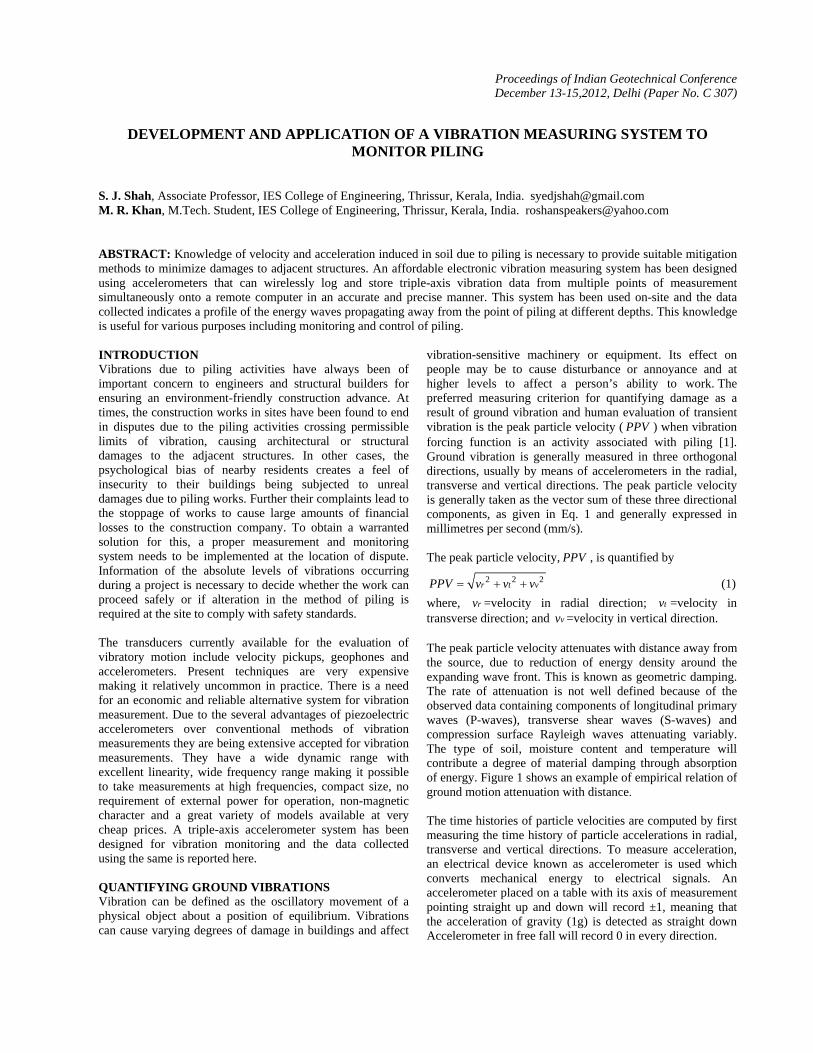
logging is implemented for avoiding possible manual reading errors. Selectable ranges of + 1.5g or + 6g are available for either a mode of high accuracy of measurement or for intense ranges of 'g'. Screw-type board mountings and coupling to ground is adopted for ensuring most precise vibrations with ground [1,2]. The system conforms requirements to be met by a vibration measuring instrument, specified in IS 14884:2000. Compact size of 15x10x10cms and a weight of just 300 grams per accelerometer module ensures maximum portability. The system is highly economic, simple to operate and precise compared with current products in industry having similar capabilities costing around 10-20 times. Data Measurement and Transmission Each accelerometer module consists of an MMA7260Q accelerometer mounted onto a PCB (Printed Circuit Board), processing done using an Atmega 328 microcontroller and data communication through a wireless serial communication RF modem based on Chipcon IC(CC2500). The accelerometers are powered using 9V rechargeable batteries. A recharging point is provided on the accelerometer module for easy recharge of the module battery after every drain out during continuous usage, using a 12V input power supply. A power on/off switch is provided to conserve battery during non-use time. Basically, accelerometers are manufactured such that they sense any minute tilt with the reference X, Y and Z axes once they are powered. It is possible that errors may arise during the field installations of accelerometer module if it is tilted or not placed properly. To account this, a calibration switch is provided on the module such that once the instrument is mounted in location of measurement, it will set the initial reading as the reference and then take further readings accordingly. The microcontroller coding is done in standard Arduino programming language compiler and boot loader, running on board to measure the triple-axis accelerations and its time interval. Data Reception and Monitoring The data sent from accelerometer modules are received by a serial communication RF modem connected to the computer via. COM port communication. Wired conversions are done for power and data connections such that all connections can be established from modem to computer through standard USB ports itself to assure easier system plug-in. The module works in half-duplex mode, meaning it can either transmit or receive but not both at same time. After each transmission module is switched to receiver mode automatically. It has internal 64 bytes of buffer for incoming data. Figure 3 shows the executable software program interface developed for displaying and storing real-time vibration data from all four accelerometer sensors simultaneously through the modem. Data storage is done in standard .xls file format to ensure easy accessibility and low storage space requirement.

Development and application of a vibration measuring system to monitor piling

Fig. 3 Software interface to display real-time vibration data Mounting Technique The technique of mounting an accelerometer affects the measurements made [2]. While it may be convenient to mount a sensor onto the casing with a cyano-acrylate adhesive such as a super glue, a magnet, or even double-sided tape, the most accurate measurements are obtained by screwing the sensor to a stud mounted onto the casing structure. Figure 4 shows how the various methods of mounting influence accuracy of accelerometer measurements [2]. The method of mounting adopted in designed vibration measurement system is to screw the sensor onto the stud on casing, to ensure most accurate results.

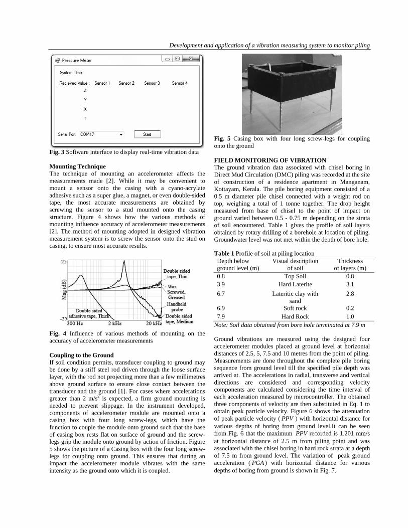
Fig. 4 Influence of various methods of mounting on the accuracy of accelerometer measurements Coupling to the Ground If soil condition permits, transducer coupling to ground may be done by a stiff steel rod driven through the loose surface layer, with the rod not projecting more than a few millimetres above ground surface to ensure close contact between the transducer and the ground [1]. For cases where accelerations greater than 2 m/s2 is expected, a firm ground mounting is needed to prevent slippage. In the instrument developed, components of accelerometer module are mounted onto a casing box with four long screw-legs, which have the function to couple the module onto ground such that the base of casing box rests flat on surface of ground and the screw-legs grip the module onto ground by action of friction. Figure 5 shows the picture of a Casing box with the four long screw-legs for coupling onto ground. This ensures that during an impact the accelerometer module vibrates with the same intensity as the ground onto which it is coupled.

Fig. 5 Casing box with four long screw-legs for coupling onto the ground FIELD MONITORING OF VIBRATION The ground vibration data associated with chisel boring in Direct Mud Circulation (DMC) piling was recorded at the site of construction of a residence apartment in Manganam, Kottayam, Kerala. The pile boring equipment consisted of a 0.5 m diameter pile chisel connected with a weight rod on top, weighing a total of 1 tonne together. The drop height measured from base of chisel to the point of impact on ground varied between 0.5 - 0.75 m depending on the strata of soil encountered. Table 1 gives the profile of soil layers obtained by rotary drilling of a borehole at location of piling. Groundwater level was not met within the depth of bore hole. Table 1 Profile of soil at piling location Depth below ground level (m)

Visual description of soil

Thickness of layers (m)

0.8 Top Soil 0.8 3.9 Hard Laterite 3.1 6.7 Lateritic clay with

sand 2.8

6.9 Soft rock 0.2 7.9 Hard Rock 1.0

Note: Soil data obtained from bore hole terminated at 7.9 m Ground vibrations are measured using the designed four accelerometer modules placed at ground level at horizontal distances of 2.5, 5, 7.5 and 10 metres from the point of piling. Measurements are done throughout the complete pile boring sequence from ground level till the specified pile depth was arrived at. The accelerations in radial, transverse and vertical directions are considered and corresponding velocity components are calculated considering the time interval of each acceleration measured by microcontroller. The obtained three components of velocity are then substituted in Eq. 1 to obtain peak particle velocity. Figure 6 shows the attenuation of peak particle velocity ( PPV ) with horizontal distance for various depths of boring from ground level.It can be seen from Fig. 6 that the maximum PPV recorded is 1.201 mm/s at horizontal distance of 2.5 m from piling point and was associated with the chisel boring in hard rock strata at a depth of 7.5 m from ground level. The variation of peak ground acceleration ( PGA ) with horizontal distance for various depths of boring from ground is shown in Fig. 7.

S. J. Shah & M. R. Khan

Fig. 6 Attenuation of peak particle velocity with distance

Fig. 7 Variation of peak ground acceleration with distance Table 2 gives the typical vibration criteria addressing building damage [3]. Comparing the obtained maximum value of 1.201 mm/s to the maximum values of particle velocity recommended, it indicates that the piling activity may be of concern to very sensitive structures such as ancient and historic buildings or structures that are visibly damaged. For transient or impact vibration, the human response to vibrations has a threshold of perception at 0.3 mm/s, becomes ‘disturbing’ at 7 mm/s and ‘very disturbing’ above 25 mm/s [4]. Whilst majority of measurements are above the perception threshold of 0.3 mm/s, none of them shall be regarded ‘disturbing’ since they are well under the specified limit of 7 mm/s.

Table 2 Typical vibration criteria to address building damage Category Particle Velocity (mm/s)Industrial buildings 100 Residential 50 Residential, New construction

50

Residential, Poor construction

25

Residential, Very poor construction

12.5

Buildings visibly damaged

4

Historic buildings 3 Historic and ancient buildings

2

CONCLUSIONS A vibration measuring system has been designed using triple-axis accelerometers, with the capability to monitor vibrations associated with piling activities in various soils. At the site where monitoring was done, the peak particle velocity was found to be attenuating with horizontal distance away from point of boring, for any depth of boring. It was found that the values of particle velocities were lowering with increased depth from surface of ground up to certain depth and again rising substantially when the depth of boring was approaching stronger rock strata. The peak ground accelerations were found to be lowering with horizontal distance away from point of boring, except for the strata of hard rock where acceleration was found to have a sudden peak and then decaying to lower values. The acceleration profiles were almost similar for lower depths from ground surface, after which the measurements in soft and hard rock strata were found varying significantly. Vibration data at the particular site was monitored effectively using developed measuring system and the vibration levels were found to be safe enough to pose no damages to the structures adjacent. The system is precise, simple to operate and affordable to almost every construction organizations or authorities of investigations to provide information on the absolute levels of vibration in cases of disputes at construction locations. REFERENCES 1. Bureau of Indian Standards (2000), Mechanical

Vibration and Shock - Vibration of Buildings - Guidelines for the measurement of vibrations and evaluation of their effects on buildings, IS 14884: 2000.

2. Romanchik, D. (2003), Guidelines for selecting an accelerometer, Application Brochure, KI 8.002e, Kistler Instrument Corp., Amherst, NY.

3. Amick, H. and Gendreau, M. (2000), Construction vibrations and their impact on vibration-sensitive facilities, Proc. Construction Congress 6, ASCE, Orlando, Florida, February, 758-767.

4. Wiss, J. F. (1981), Construction vibrations: State of the art, Journal of the Geotechnical Division, ASCE, Vol. 94 No.9, 167-181.

Proceedings of Indian Geotechnical Conference December 13-15, 2012, Delhi (Paper No. C 308.)

EFFICACY OF INSTRUMENTATION FOR DISTRESSED CONCRETE GRAVITY DAM

R.K. Mathur, Central Soil and Materials Research Station, New Delhi. rmathur@nic.in Rajbal Singh, Central Soil and Materials Research Station, New Delhi. rajbal.singh@nic.in

ABSTRACT: The distress in Rihand concrete dam is due to the alkali-aggregate reaction. The expansion of concrete has prompted to cracking of concrete and consequently difficulty in operation of spillway gates, snapping of reinforcement bars of the concrete columns, smooth running of turbine in the surface powerhouse at the downstream etc. It was, therefore, decided to monitor the cracks in the dam and appurtenant structures with the help of suitable instruments. This paper deals with the case study of distress at Rihand dam project and implementation of instrumentation programme to monitor the distress due to opening and closing of the joints/cracks by crack monitor and deflection of dam structures by plumb line. The instrumentation was planned for evaluating the remedial measures required in the dam and powerhouse. INTRODUCTION Rihand dam is a concrete gravity dam of 934.45 m length and 91.96 m height. It taps river Rihand which is a tributary of river Sone and the project is situated in District Sonebhadra of Uttar Pradesh state. The dam comprises of 61 independent blocks of widths ranging from 12.8 m to 18.3 m with ungrouted joints. Block numbers 28 to 33 constitute intake and powerhouse, while the spillway is on blocks 34 to 47 and the rest are non-overflow blocks. The powerhouse is located at the toe of the dam, and was commissioned in 1962 with 5 units of 50 MW each, with a provision for the sixth machine which was added in 1966 with total installed capacity of 300 MW. The view of the Rihand dam along with surface powerhouse is shown in Fig. 1.

Fig.1 Down stream view of Rihand dam along with surface powerhouse A reinforced concrete structure connects the toe of the dam with the powerhouse. The transformers are placed on the top most floor of this framed structure. The load of the transformers is being transferred directly to the dam toe through separate columns. The penstock gallery is housed in this framed structure, which separates the powerhouse structure through a 25 mm thermocole filled joint. The quantity of concrete used in the gravity dam and appurtenant works was of the order of 16, 80,000 cubic meters.

This paper deals with the case study of distressed Rihand concrete dam and surface power house and implementation of instrumentation programme to monitor the opening and closing of the joints/cracks and deflection of dam structure. FOUNDATION GEOLOGY The rocks at Rihand site are essentially granite, massive to thinly foliated granite gneiss and injection gneiss. Minor bands of phyllite, schist, amphibolites and quartzite are also present within the bed rock at the dam site. The dam is founded on gneissose granite, while the powerhouse is founded on injection gneiss with bands of dioritic rock, amphibolites and mica schist. The contact zones of the granite and injection gneiss are sheared at places. THE DISTRESS Cracks had been, in fact, noticed in different concrete structures, since the time when dam and powerhouse were commissioned in 1962. Within a decade of commissioning of the project, the distress of the structure became alarming. Since 1972, generating units frequently tripped due to high spill current. The distress mentioned above became excessive, requiring immediate remedial actions for generating electricity. The following distress in the dam and related structures were significant and indicated the scenario of general distress: • Dam

- Excessive deformation and bulging of spillway piers. - Difficulty in operation of crest and penstock gates due to

shifting of guide rails. - Cracks on the upstream face of the dam, intake structure

and various galleries. • Powerhouse

- Tilting of generating shaft. - Snapping of reinforcement and deformation in penstock

gallery frame columns. - Tilting and deformation of draft tube structure. - Difficulty in operation of overhead gantry crane and draft

tube crane.

R.K. Mathur, Rajbal Singh,

PERFORMANCE MONITORING The distress monitored during initial stages did not attract any special attention and hence there was no special response to distress. However, the instruments installed at the time of construction of the dam and appurtenant works were there. These instruments included thermometers, strain meters, stress meters, joint meters, deflection meters and instruments for the measurement of uplift pressure. Deflection of the dam axis was being measured with the help of plumb line with mirror-scale arrangement. However, all these instruments had become in-operational by seventies. The observations available for the initial period after construction were analyzed and data did not reveal any unusual trend indicating structural distress or instability. The problem had become quite acute and the senior officers of Irrigation Department of U.P., inspected the dam in 1973, and the remedial measures suggested by them were carried out by the field engineers. The following studies were taken up in accordance with the recommendations of the Expert Committee in August 1984: • Study of expansion of cement concrete. • Geodetic survey of dam by Survey of India. • Finite element analysis of the dam section by Central

Water Commission, New Delhi. • Geological studies of the dam by Geological Survey of

India, Lucknow. • Monitoring of dam and appurtenant works by Central

Soil and Materials Research Station, New Delhi. The most important finding of the above studies was expansion of concrete. Expansion of concrete was due to alkali-aggregate reaction. Some details of the distress are described in [1]. The following major remedial measures were suggested by Rihand Dam Experts Committee: • Emergency passenger lift located in shaft of the block 34

at RL 830 ft to be closed by concrete and the cracks grouted, which was done in 1985.

• To release any uplift pressure coming on the foundation rock, the 4 inch diameter uplift pressure pipes provided in the foundation gallery were cleaned by compressor.

• The penstock gallery columns showing distress were rehabilitated by epoxy grouting and steel jacketing during 1985-87.

• The interaction of the dam and penstock gallery frame with the mass concrete of powerhouse was done away by making the expansion joint between the penstock gallery frame and powerhouse functional through the removal of thermocole.

• To minimize the ingress of water, the upstream face was treated by injecting epoxy resin and subsequently painting the upstream face.

The cracks and joint in the dam body and the powerhouse are shown in Figs. 2 and 3 along with the installed 3-dimensional crack monitors for measuring the movements in the cracks/ joints. The deterioration of the concrete is also seen in Fig. 2.

Fig. 2: Crack at Erection Bay Turbine unit No. 1

Fig. 3 Crack and crack monitor at spillway joint on dam top between blocks 35 and 36. INSTRUMENTATION BY CSMRS The Central Soil and Materials Research Station (CSMRS), New Delhi has taken up instrumentation work for crack deformation monitoring in 1986. The cracks at 32 locations are being monitored with the help of vernier gauges and 3D crack monitors (Figs. 4 and 5).

Fig. 4 3-Dimentional crack monitor The 3-D crack monitor (Fig. 4) is capable of measuring crack deformations in three mutually perpendicular directions. X-axis measures the deformation along the crack i.e. the shear movement of the crack. Y-axis measures the deformation across the crack or perpendicular to the crack. The opening and closing of the crack/joint can be measured by Y-axis. Z-axis measures the deformation of the two walls of the crack/joint perpendicular to X and Y axes as shown in Fig. 5. The crack monitor is light weight, portable, compact and is very easy to install.

Efficacy of instrumentation for distressed concrete gravity dam

Fig. 5 3-Dimentional Crack Monitor 3-D Crack Monitoring Three-dimensional monitoring on dam top and in powerhouse complex is being done by 3D crack monitor at 10 locations. Crack deformations monitoring by 3D crack monitors are shown in Figs. 6 on cracks and existing joints.

Fig. 6 Variations of deformations with time at Y-axis of the crack/joint by 3D crack monitor.

The crack monitor 3-D/10 installed as dummy for taking into considerations the instrument material expansion and contraction due to coefficient of expansion of material. On analyzing the data, it is observed that maximum deformation among all 10 locations is in Y direction, which is 12.02 mm at 3D/6 location at EL 622 feet on Column No. 6 (D/S Wall). Minimum deformation is in X direction, which is -5.62 mm at 3D/8 location (EL 622 feet on Column 22 (D/S Wall) [2]. This shows that both maximum and minimum deformations are at EL 622 feet on columns. Other Significant Observations The movement across the crack have further been analyzed as shown in Figs. 7 and 8 at lower and higher elevations (up to 622 ft. and above 680 ft.) respectively [3]. The deformations at elevation 622 ft as shown in Fig. 7 are significant and are in increasing order with time. It shows the effect of distress in the dam body as well as in the powerhouse and needed to be taken care. The deformations at elevation 683 ft as shown in Fig. 8 are also very significant and are increasing and decreasing with time i.e. opening and closing of the joint/cracks. This variation at higher elevation is due to distress and variation in reservoir water level as also discussed by [4].

Fig. 7 Variations of deformations with time at Y-axis of the crack/joint at lower elevations (622 ft)

Fig. 8 Variations of deformations with time at Y-axis of the crack/joint at higher elevations (683 ft)

Analysis of Crack Deformation and Deflection With Respect to Reservoir Water Level The time gap between crack deformation and peak reservoir water level w.r.t. time was analysed. Similar analysis was also done for deflection variation in correlation with peak reservoir water level. As shown in Table 1 and Fig. 9, it is observed that crack deformation follows reservoir water level and time lagging between peaks of water level and crack deformation variation are between 53 to 126 days [4] during monitoring period from May 1998 to February2012. Similarly time lagging between peaks of reservoir water level and deflection variation are between 91 to 159 days during monitoring period from August 2001 to February 2012 shown in Fig. 10 and time lagging given in Table 2. Similarly time lagging between peaks of reservoir water level and deflection variation are between 91 to 159 days during monitoring period from August 2001 to February 2012 shown in Fig. 10 and time lagging given in Table 2.

R.K. Mathur, Rajbal Singh,

Table 1: Time lagging between crack deformation and reservoir water level at peaks

Date of reaching at peak water level/ max. deformation

Time lagging (days) Reservoir water

level Crack deformation

( 3D/3; Y-axis) 09/10/98 07/02/99 121

05/11/99 13/01/00 69

12/10/00 01/02/01 112

22/08/01 26/12/01 126

17/10/02 09/12/02 53

19/09/03 10/12/03 82

19/08/04 19/10/04 61

20/09/06 17/01/07 121

06/11/07 18/12/07 42

10/09/10 21/10/10 41

19/10/11 01/02/12 105

Fig. 9 Deformation (Y axis) and reservoir water level verses time from 3-D crack monitor

Fig. 10 Deflections and reservoir water level verses time from plumb line CONCLUSION It is concluded that the deformations at lower elevation (622 ft) are significant and are in increasing order with time

irrespective of fluctuations in reservoir water level. It shows the effect of distress in the dam as well as in the powerhouse. The deformations at higher elevation (683 ft) are in increasing and decreasing order with time and fluctuation in reservoir water level. Opening and closing of the joint/cracks can be related with reservoir water level. Crack deformations by crack monitor follow the pattern of reservoir water level with time lagging between crack deformation and reservoir water level around 2-4 months. It is also observed that pattern of deflection by normal plum line also follows the pattern of reservoir water level and time lagging between maximum deflection and peak reservoir water level is around 2-5 months. It is confirmed from the monitoring by crack monitor and normal plumb line that maximum deformation in cracks and deflections in dam is attained in 2 to 5 months time after peak reservoir water level. Table 2: Time lagging between deflection and reservoir water level at peaks

REFERENCES 1. Sudhindra, C. and Sharma, V.M. (1989).

Instrumentation- A potential tool for performance surveillance of Rihand dam, International Workshop on Research Needs in Dam Safety, New Delhi, pp. 255-259.

2. CSMRS (2012), Report on the instrumentation for crack deformations in Rihand dam (UP) – structural behaviour monitoring, Central Soil and Materials Research Station, New Delhi, March 2012, India.

3. Singh Rajbal and Mathur R.K. (2003) “Distress in concrete dam and instrumentation” ‘Hydrological & geotechnical instrumentation for water resources project’, National Water Academy (NWA), Pune.

4. Sharma V.M., Singh R.B., and Abdullah H., (1991) “Instrumentation for detecting of Ageing at Rihand dam in India”, 17th of the International Commission on Large Dams, Vienna, pp. 827-835.

Date of reaching at peak water level/max. deflection

Time lagging (days) Reservoir

water levelDeflection monitored from Plumb Line

05/10/2001 04/01/2002 91

16/09/2002 20/01/2003 126

21/09/2003 25/11/2003 65

24/07/2004 30/12/2004 159

17/09/2005 16/01/2006 121

03/09/2006 28/01/2007 147

09/10/2007 06/03/2008 159

07/09/2008 10/02/2009 156

12/09/2009 08/01/2010 118

07/10/2010 20/01/2011 105

25/09/2011 31/01/2012 128

Proceedings of Indian Geotechnical Conference December 13-15, 2012, Delhi (Paper No. C310)

DEVELOPMENT OF SIMPLE FIELD TECHNIQUE FOR CHARACTERIZATION OF SOIL Arun perumal P, P.G student, Anna University, Chennai - 600 025, India. E-mail: arunperumal2000@yahoo.co.in Ilamparuthi K, Professor and Head, Anna University, Chennai - 600 025, India. E-mail: kanniilam@gmail.com.

INTRODUCTION

The aim of this research work is systematic study on light cone penetration test (LCPT) in sand and clay deposits independently in order to bring out its utility as a tool for subsurface investigation of shallow depths. A subsurface investigation device should provide required strength and compressibility parameters either by direct measurements or indirect correlations. As a penetration device direct measurement of strength parameters is not simple. Hence it is decided to develop indirect correlation. Such correlations are available for Standard Penetration Test (SPT). However SPT could not be used effectively in week deposit like soft clay and dynamic nature of this test develops pore pressure during penetration. To overcome this limitation static cone penetration (SCPT) is been employed. Despite the applicability of these two field testing methods have been well established, the geotechnical engineers are involved in developing simple field testing equipment. One such device is light cone penetration test (LCPT) Anbu (2001) proposed a method to determine the penetration resistances using a cone of 30mm dia and the resistances were utilized to evolve possible correlation with LCPT resistance, SPT and SCPT resistances. The light cone penetration test results of 25mm and 30mm dia cone are compared and effect of size of cone was analysed. Naga et al (2011) proposed a simple method for evaluating the effect of rod skin friction on dynamic cone penetration test results in cohesive soils. This method is simple and requires neither additional equipment nor special test procedures, and thus represents an improvement on existing dynamic probing practice in the field testing. Gandhi et al. (1998) made use of light cone penetration test to evaluate densification of pond ash at Mettur Thermal Power Plant by blasting. Static cone penetration tests were also carried out along with LCPT tests. The cone resistances of SCPT are correlated with LCPT 'N' values. Further the light cone penetometer is not employed widely as a tool for soil investigation and also for evaluation of strength parameters. Therefore, this equipment needs standardization for developing generalized correlations with other types of standard penetrometers and strength properties of soils.

EXPERIMENTAL SETUP AND PROCEDURE

The Experimental setup of light cone penetrometer device developed in this study is as shown in Fig 1. The total weight of the device is 45kg. The penetrometer devised for the study consists of the following components.

a) Cone b) Driving rod c) Drive head assembly d) Hammer e) Base plate, and f) Guide Stand

The location of penetration test (LCPT) is marked on the ground. The top surface of the ground is cleaned and leveled to seat the base plate. The cone with a driving rod is passed through the collar of the base and positioned vertically. Guide rod assembly is then attached to the driving rod. Hammer of 15 kg is slipped through the guide rod and positioned on the top of the drive head. During the process of driving, the cone and the drive rod assembly is held vertically in position with the help of a guide stand. Number of blows required for every 5cm penetration is counted and recorded. Hammering is done continuously at the rate of 15blow/minute. After complete penetration of the first driving rod, the hammer and the guide rod are removed and the length of the driving rod is extended by attaching another rod. The driving of the cone is continued by adopting the procedure explained above. The process of driving is continued till the number of blows exceeds 25 blows per 5 cm penetration or maximum depth of investigation of 6 meters. After the test is completed, the hammer and drive head are detached from the drive rod. Hammer is then inserted to the drive rod and the drive head assembly is again fixed. By back hammering the drill rods are withdrawn. The procedure explained above adopted for driving the cone to desired depth to measure the resistance of soil at that depth. To measure the static load resistance the cone is driven into the soil by hammering after reaching the desired depth the cone is loaded statically by applying load on to the cone through bearing plate using slotted plates of known weights. The movement/settlement of cone assembly is measured using dial gauges till the settlement of 20mm. Fig 1 a) shows the Static load test and Fig 1 b) shows driving arrangement of testing systems in the field.

ABSTRACT: In this paper a simple Light Cone Penetrometer was devised to establish suitable recommendations on test procedure both for clay and sand deposits, interpretation of results and possible correlation with standard penetration tests. The strength of soil obtained through field tests are compared with strength measured in the laboratory on undisturbed samples and provided LCPT ‘N’ based correlation for assessing strength parameter of soil.

Ilamparuthi R.K & Arun perumal P,

a) Static load test b) Penetration test by Driving

Fig.1 Details of arrangements for light cone penetration test

LABORATORY TESTS

In addition to penetration test, undisturbed samples were also collected at different locations and depths along with the split barrel samples. These samples were tested in the laboratory for index properties and the strength as per relevant codal provisions. The samples tested are classified based on IS 1498-1970. In case of sandy deposits, field density tests were also carried out at top layers within the depth of 1 m from the ground level. The direct shear tests were carried out on representative sand samples by compacting them at densities correspond to respective field densities.

FIELD TEST RESUSTS The LCPT resistances were obtained by adopting the procedure explained. These tests were conducted at 29 locations covering different areas in and around Chennai where deposits were either dominantly sand or clay. At all these locations tests were conducted to a maximum depth of 6m or resistance should not exceed 25 blows. At each location standard penetration test was also conducted with a view to establish the correlation between them. Theoretical ratio of SPT and LCPT penetration resistance is established based on the energy which is as follows

N = 0.62NLCPT (1)

Typical field test results for dominantly clay and sand stratum of Chennai are shown in Fig.2 and Fig.3 respectively along with the soil profile of the respective area. The resistances of both the methods are compared and can be seen that they show almost similar trend with penetration depth irrespective of soil type. But light cone penetration resistances are lighter than standard penetration resistance. Almost similar trend is seen from tests conducted at 29 locations. However LCPT resistance are more sensitive and they are efficient in identifying thin layers of soil deposit with low resistance (weaker deposits) but presence of coarse particles records unreasonably high resistance, which provides misleading condition of deposit.

Fig.2 Variation of LCPT and SPT resistance with depth at Korukkupet, Chennai in sandy startum.

Fig.3 Variation of LCPT and SPT resistance with depth at Maduravoyl, Chennai. in clayey stratum CORRELATION BETWEEN SPT AND LCPT Analysis of LCPT results and the corresponding SPT results in field reveals a good correlation between them. The correlation coefficient of 0.71 is obtained from the graph and the total statistical variance (R2 ) value is 0.93 for sand with fines less than 25%. The correlation coefficient of 0.69 is obtained for the clay and the total statistical variance (R2 ) value is 0.96 as shown in Fig.5.

Fig.4 Relation between N and NLCPT for sand

DEVELOPMENT OF SIMPLE FIELD TECHNIQUE FOR CHARACTERIZATION OF SOIL

Fig.5 Relation between N and NLCPT for clay

The correlation obtained between the field N value with LCPT N value for sand and clay is as follows.

Sand: N = 0.71 NLCPT (2)

Clay: N = 0.69 NLCPT (3)

Based on the correlation presented, it can be said that the ratio between SPT N and LCPT N is 0.7. This value is marginally higher than the value of 0.62 obtained based on driving energy. The influence of relative density and consistence of sand and clay deposits respectively on penetration resistance is analyzed with the help of existing SPT ‘N’ correlation with consistency/ relative density. The correlation thus established is presented in Table1.

Table.1 Comparison of LCPT and SPT results

RELATION BETWEEN Φ AND NLCPT FOR SAND.

In sandy stratum the LCPT resistance generally correlates well with the SPT resistance except the results obtained from the sand layer of SP-GP stratum. Therefore the test results of such locations were neglected for the determination of the relation between shear strength and LCPT resistance. The

relation obtained from the graph presented in Fig.6 is as below. Φ = 0.29NLCPT + 25º (4)

Fig.6 Relations between Φ and NLCPT for sand

RELATION BETWEEN CU AND NLCPT FOR CLAY.

The relation between the cohesive strength and the LCPT resistance is shown in Fig.7. The relation between them is linear with statistical variance (R2) of 0.96.The undrained strength parameter Cu can be obtained from the LCPT ‘N’ by the relation given below

Cu ( kN/m2) = 4.21 NLCPT

(5)

Fig.7 Relation between Cu and NLCPT for clay

LCPT STATIC LOAD TEST IN CLAYEY STRATUM:

The special equipment for the pushing test was designed and fabricated for the estimation of Cu in a prepared clay bed in the laboratory. The test set up, arrangement of equipment and method of testing are described in detail in the previous section the details of test bed as shown below. Results of pushing resistance in laboratory correlate reasonably with the Cu value arrived from van shear test. As reasonable correlation obtained in laboratory, the test set up was used in

Type of soil

LCPT

(NLCPT)

SPT

(N) Relative density/

consistency

Sand

0 - 5

5 - 15

14 - 25

0 - 4

4 - 10

10 - 30

Very Loose

Loose

Medium Dense

Clay 0 - 3

3 - 5

5 - 11

10 - 20

>20

0 - 2

2 - 4

4 - 8

8 - 15

15 - 30

Very soft

Soft

Medium stiff

Stiff

Very stiff

Ilamparuthi R.K & Arun perumal P,

field along with LCPT. The Cu values are arrived from the pushing resistance using the formula give below.

cu = (σ1 – γ’d)/6 (6)

where cu = cohesion of the clayey layer, kN/m2

σ1 = applied pressure, kN/m2

γ’d = effective overburden pressure, kN/m2

d = depth of test

The maximum static load of 162kg was used for the penetration in stiff clay and load of 50 kg was used for the penetration in soft clay stratum. The variation of undrained cohesion obtained using SPT ‘N’ and LCPT ‘N’ for all the clay locations are compared. The undrained cohesion obtained in the field from the static load Cu(LCPT) is compared with the undrained cohesion obtained through SPT ‘N’ value Cu(N). Cu(N) is determined using the empirical equation of NAVFAC 7.02, Terzhagi and Bowles from SPT N value . There is reasonable agreement between the Cu(LCPT) from pushing test and Cu(N) obtained from Bowels empirical equation. Therefore Cu(LCPT) is compared with the bowels empirical equation. The relation between Cu(LCPT) and Cu(N) is shown in the Fig.8.

Fig.8 Relation between Cu(N) vs Cu(LCPT)

The relation between the Cu obtained from LCPT and Cu from SPT is as follows.

Cu (LCPT) = 1.14 Cu(N) (7)

It is observed that undrained cohesions obtained by Bowles relation are very close to the value of undrained cohesion obtained from LCPT with a maximum variation of 11%. CONCLUSION

The study aims at making site characterization and evaluation of strength parameters economically by a simple method. In this study a simple device named light cone penetrometer is devised to imply in the place of SPT in which employing heavy SPT hammer may not record accurate blow count of resistance due to possible over driving of the penetrometer.

The LCPT resistance measured in sand and clay of various sites are almost follows the soil resistance trend obtain through SPT. However the LCPT test is more sensitive tool, which can identify localized weaker deposit. But this may lead to higher resistance when come across or penetration in large size particles like gravel. Overall it can be said that the light cone penetration device developed in this study can be utilized not only as an aid to know the soil type and relative compactness of the deposits but also for evaluation of strength parameters. By virtue of its simplicity, versatility and economy in operation, this can be gainfully employed in soil investigation for shallow depths. It was felt essential that the study could be extended to cover more potential sites in improving correlations recommended.

REFERENCES

1.Anbu K.(2001),“Light cone penetration test and interpretation of its data”, M.E Thesis,Anna university..

2. Naga A-H.M., Holtrige M., and Pender M.J. (2011), "Simple method for correcting dynamic cone penetration test results for rod friction",Geotechnique Letters 10.1680/geolett.11.00012.

3.Gandhi, S.R, Dey A.K., Sharma S., Selvam S. (1998), “the application of light cone penetration test to evaluate dezincification of pond ash by blasting” Indian Geotechnical Conference , 1998, December, pp.7-10.

4. Bowles (1997),“Foundation Analysis & Design”, The Mc Graw-Hill companies Inc.

Proceedings of Indian Geotechnical Conference December 3-15, 2012, Delhi (Paper No. C312)

THE SEISMIC DILATOMETER FOR IN SITU SOIL INVESTIGATIONS S. Marchetti, Prof., L’Aquila University – Italy, silvano@marchetti-dmt.it ABSTRACT: In the last decades we have assisted at a considerable shift from laboratory testing to in situ testing, to the point that, today, in situ testing is often the major part of a geotechnical investigation. The State of the Art at the last Geotechnical World Conference in 2009 indicates that direct-push in situ tests, such as the Cone Penetration Test (CPT) and the Flat Dilatometer Test (DMT), are fast and convenient in situ tests for routine site investigation. Scope of this paper is to describe the DMT, the obtained information and engineering applications. The paper also describes the recently developed Seismic Dilatometer (SDMT). The SDMT is a DMT with an add-on seismic module for measuring also the shear wave velocity Vs. DMT and SDMT have been found helpful in projects where soil stiffness and settlements predictions are critical to the design. INTRODUCTION The Flat Dilatometer (DMT) is an in situ testing tool developed some 30 years ago [1]. The DMT is currently used in practically all industrialized countries. It is standardized in the ASTM [2] and the Eurocode [3]. The DMT has been object of a detailed monograph by the ISSMGE Technical Committee TC16 [4]. Some key features of the DMT are : • The DMT is a penetration test. As such, it has the

advantage of not requiring a borehole. • The DMT, being a load-displacement test, provides

information on soil stiffness, an information unobtainable by penetration tests, that essentially measure “rupture” characteristics, i.e. strength. Moreover the insertion distortions caused by the DMT blade are substantially less than the distortions caused by conical probes.

• The DMT equipment is robust, easy to use and remarkably operator-independent and repeatable.

• The DMT provides information on Stress History, whose knowledge is of primary interest, because Stress History has a dominant influence on soil behavior.

As to the SDMT, the add-on module has added to the parameters measurable by DMT the shear wave velocity VS. VS is today increasingly measured because of: • More frequent requirement of seismic analyses, for which

VS is a basic input parameter. • The newly introduced Eurocode 8 seismic regulations

prescribe the determination of VS in the top 30 m at all construction sites located in the seismic zones.

• SDMT provides both the Go stiffness at small strains (the shear modulus G0 = ρ VS

2) and the stiffness at operative strains (as represented by the constrained modulus MDMT). Such two stiffnesses may offer guidance when selecting the G-γ curves, i.e. the decay of the shear modulus G with the shear strain γ.

DILATOMETER TEST (DMT) The flat dilatometer consists of a steel blade having a thin, expandable, circular steel membrane mounted on one face.

When at rest, the membrane is flush with the surrounding flat surface of the blade. The blade is connected, by an electro-pneumatic tube running through the insertion rods, to a control unit on the surface (Fig. 1). The control unit is equipped with pressure gauges, an audio-visual signal, a valve for regulating gas pressure (provided by a tank) and vent valves. The blade is advanced into the ground using common field equipment, i.e. penetrometers normally used for the cone penetration test (CPT) or drill rigs. The DMT can also be driven, e.g. using the SPT hammer and rods, but statical push is by far preferable. Pushing the blade with a 20 ton penetrometer truck is most effective (up to 80 m of profile per day). The test starts by inserting the dilatometer into the ground. When the blade has advanced to the desired test depth, the penetration is stopped. The operator inflates the membrane and takes, in about 30 sec, two readings: the A pressure, required to just begin to move the membrane (‘lift-off’ pressure), and the B pressure, required to expand the membrane center of 1.1 mm against the soil. A third reading C (‘closing pressure’) can also optionally be taken by slowly deflating the membrane soon after B is reached. The blade is then advanced to the next test depth, with a depth increment of typically 20 cm. The interpretation proceeds as follows. First the field readings are converted into the DMT intermediate parameters ID, KD, ED (Material index, Horizontal stress index, Dilatometer modulus). Then ID, KD, ED are converted, by means of commonly used correlations, to: constrained modulus M, undrained shear strength Cu, Ko(clays), OCR (clays), friction angle Ø’ (sands), bulk unit weight. Consolidation and permeability coefficients may be estimated by performing dissipation tests [4]. The C-reading, in sand, approximately equals the equilibrium pore pressure. An example of the profiles obtained by DMT is shown in Fig. 3a, where :

- ID is the material index, that gives information on soil type (sand, silt, clay)

-M is the vertical drained constrained modulus (at geostatic stress)

S. Marchetti

-Cu is the undrained shear strength - KD is the Horizontal Stress Index. The profile of KD is similar in shape to the profile of the overconsolidation ratio OCR. KD ≈2 indicates in clays OCR = 1, KD > 2 indicates overconsolidation. The KD profile often provides, at first glance, an understanding of the Stress History of the deposit.

More detailed information on the DMT equipment, test procedure and all the interpretation formulae may be found in the comprehensive report by the ISSMGE Technical Committee TC16 [4]. SEISMIC DILATOMETER TEST (SDMT) The SDMT is the combination of the flat dilatometer with an add-on seismic module for the measurement of the shear wave velocity [5-9]. The seismic module (Fig. 2a) is a cylindrical element placed above the DMT blade, equipped with two receivers located at 0.5 m distance. When a shear wave is generated at surface, it reaches first the upper receiver, then, after a delay, the lower receiver. The seismograms acquired by the two receivers, amplified and digitized at depth, are transmitted to a PC at the surface, that

determines the delay. Vs is obtained (Fig. 2b) as the ratio between the difference in distance between the source and the two receivers (S2 - S1) and the delay from the first to the second receiver (Dt). The true-interval test configuration with two receivers avoids possible inaccuracy in the determination of the “zero time” at the hammer impact, sometimes observed in the pseudo-interval one-receiver configuration. Moreover, the couple of seismograms recorded by the two receivers at a given test depth corresponds to the same hammer blow. The repeatability of the Vs measurements is remarkable (observed Vs repeatability ≈ 1 %, i.e. a few m/s). Fig. 2c shows an example of seismograms obtained by SDMT at various test depths at the site of Fucino. Fig. 3a shows an example of SDMT results. The fifth diagram is the Vs profile obtained by the seismic module. TESTABLE SOILS The soils that can be investigated by DMT range from extremely soft soils to hard soils to soft rocks. The DMT readings are accurate even in nearly liquid soils. On the other hand the blade is very robust and can penetrate even in soft rock. Clays can be tested from Cu = 2-4 kPa up to 1000 kPa

(a) (b) (c)

Fig. 1 Flat Dilatometer: (a) Equipment (b) Dilatometer Blade (c) Schematic layout of the seismic dilatometer test.

Fig. 2 Seismic Dilatometer: (a) DMT blade and seismic module (b) Schematic layout of the seismic dilatometer test. (c) Example of seismograms as recorded and rephased.

(a) (b) (c)

The seismic dilatometer for in situ soil investigations (marls). The range of measurable moduli M is from 0.4 MPa

up to 400 MPa. The DMT blade can be inserted by a variety of penetration machines. Truck-mounted penetrometers are by far the fastest. A drill rig is also usable, with the Torpedo configuration [4], though at a lower productivity. Penetration by percussion, e.g. using the SPT hammer, is also possible, although not recommended. APPLICATIONS TO ENGINEERING PROBLEMS

Design via Parameters In most cases the DMT estimated parameters, in particular the undrained shear strength Cu and the constrained modulus M, are used with the common design methods of Geotechnical Engineering for evaluating bearing capacity, settlements etc. However, for a number of applications, additional specific comments may be opportune.

Settlements of Shallow Foundations. Predicting settlements of shallow foundations is probably the No. 1 application of the DMT, especially in sands, where undisturbed samples cannot be retrieved. Settlements are generally calculated by means of the one-dimensional formula (Fig. 3b) :

zM

SDMT

vDMT Δ

Δ=∑−

σ1 (1)

with Δσv calculated according to Boussinesq and MDMT

constrained modulus estimated by DMT. The validity of the method has been confirmed by a large number of observed agreement between measured and DMT-predicted settlements. Fig. 3c compares the insertion distortions caused by probes of different shape. Laterally Loaded Piles Methods have been developed for deriving P-y curves from DMT results [11,12]. A number of independent validations (NGI, Georgia Tech and tests in Virginia sediments) have indicated that the two methods provide similar predictions, and that the predictions are in quite good agreement with the observed behavior. Note that all methods are for the case of first time monotonic loading. Detecting Slip Surfaces in OC Clay The KD ≈ 2 method [4] permits to detect active or old slip surfaces in overconsolidated (OC) clay slopes, based on the inspection of the KD profiles. In essence, the method consists in identifying zones of normally consolidated (NC) clay in a slope which, otherwise, exhibits an OC profile. The NC clay bands, remoulded by the sliding, then reconsolidated under the weight of the overlying soil, are recognized by using KD ≈ 2 as the identifier of the NC zones. Note that the method involves searching for a specific numerical value (KD = 2) rather than for simply weak zones, which could be detected just as easily by other in situ tests. The KD = 2 method

Fig. 4 Curves for evaluating CRR for clean sand : (a) From Kd (Monaco 2005 [5]) (b) From Vs (Andrus & Stokoe 2000 [13]).

(a) (b)

Fig. 3 (a) Example of SDMT results (from two nearby SDMTs) (b) Settlement prediction by DMT (c) Soil distortions caused by tips of different shape (Baligh & Scott [10]).

(a) (b) (c)

S. Marchetti permits to detect even quiescent surfaces, which could reactivate e.g. due to an excavation. Monitoring Densification/ Stress Increase Before-after DMTs have been frequently used for monitoring soil densification treatments. Compaction is generally reflected by a brisk increase of both KD and MDMT. Results by various authors indicate that the percentage increase in MDMT is approximately twice the increase in qt. In other words densification increases both qt and MDMT, but MDMT increases at a faster rate. DMT appears therefore well suited to detect the benefits of the soil improvement. It may be noted that, since densification is often aimed at reducing settlements, it would appear more direct to set the specifications in terms of minimum M rather than of minimum Dr - a not precisely measurable parameter. The DMT is suitable for detecting small horizontal stress variation, e.g. in the relaxing soil behind diaphragm walls during the excavation. Liquefiability Evaluation. Fig. 4 shows two diagrams providing estimates of the Cyclic Resistance Ratio (CRR) of a clean sand (FC<5%) by DMT/ SDMT. Note that DMT provides one estimate of CRR (based on KD), while the seismic module provides a second independent estimate of CRR (based on Vs). The curve for estimating CRR from KD is by Monaco et al. [5], for estimating CRR from Vs by Andrus & Stokoe [13]. Details on the derivation and use of these curves may be found in Monaco et al. [5,6]. The use of Kd to evaluate CRR is increasing, due to the recognized sensitivity of KD to a number of factors which are known to increase liquefaction resistance – such as stress history [9], prestraining/aging [6], cementation, structure – but are difficult to sense by other tests, and by KD's relationship with the state parameter [9]. Subgrade Compaction Control DMT has been used for verifying the compaction of the natural ground surface (i.e. the subgrade) to support the road superstructure [14]. DMT has been used as an economical production tool for quality control of the compaction, with only occasional verifications by the originally specified methods. CONCLUSIONS The Flat Dilatometer is a relatively recent in situ test. It provides estimates of a variety of design parameters. It is fast and simple to operate, and the measurements are reproducible and operator independent. The DMT most frequent application is to predict settlements. Other applications have been briefly described in the paper. The test is standardized in the ASTM and the Eurocode. REFERENCES (°)

1. Marchetti, S. (1980). “In Situ Tests by Flat Dilatometer”. Jnl GED, ASCE, 106, GT3 : 299-321.

2. ASTM D6635-01 (2001 & 2007). "Standard Test Method for Performing the Flat Plate Dilatometer." Book of Standards, 14 pp.

3. Eurocode 7 (1997 & 2007). "Geotechnical Design - Part 2: Ground Investigation and Testing." EN 1997-2:2007.

4. TC16 (2001). “The Flat Dilatometer Test (DMT) in Soil Investigations”. A Report by the ISSMGE Committee TC16. May 2001, 41 pp. Reprinted in Proc. 2nd Int. Conf. on the Flat Dilatometer, Washington D.C. 2006 : 7-48.

5. Monaco, P., Marchetti, S., Totani, G. & Calabrese, M. (2005). “Sand liquefiability assessment by Flat Dilatometer Test (DMT)”. Proc. XVI ICSMGE, Osaka, 4: 2693-2697.

6. Monaco, P. & Marchetti, S. (2007). “Evaluating liquefaction potential by seismic dilatometer (SDMT) accounting for aging/stress history”. Proc. 4th Int. Conf. on Earthquake Geotechnical Engineering ICEGE, Thessaloniki, 12pp.

7. Marchetti, S., Monaco, P., Totani, G. & Marchetti, D. (2008). "In Situ Tests by Seismic Dilatometer (SDMT)" Proc. From Research to Practice in Geotechnical Engineering, ASCE Geotech. Spec. Publ. No. 180 (honoring J.H. Schmertmann) : 292-311.

8. Monaco, P., Marchetti, S., Totani, G. & Marchetti, D. (2009) “Interrelationship between Small Strain Modulus Go and Operative Modulus”. International Symposium IS-Tokyo 2009 on Performance-Based Design in Earthquake Geotechnical Engineering, 8 pp.

9. Marchetti S. (2010) "Sensitivity of CPT and DMT to stress history and aging in sands for liquefaction assessment", Proc. CPT 2010 Int.nl Symposium Huntington Beach, California.

10. Baligh, M.M. & Scott, R.F. (1975). "Quasi Static Deep Penetration in Clays". ASCE Jnl GE, 101, GT11 : 1119-1133.

11. Robertson, P.K., Davies, M.P. & Campanella, R.G. (1987). "Design of Laterally Loaded Driven Piles Using the Flat Dilatometer". Geot. Testing Jnl, Vol. 12, No. 1 : 30-38.

12. Marchetti, S., Totani, G., Calabrese, M. & Monaco, P. (1991). "P-y curves from DMT data for piles driven in clay". Proc. 4th Int. Conf. on Piling and Deep Foundations, DFI, Stresa, Vol. 1 : 263-272.

13. Andrus, R.D. & Stokoe, K.H., II. (2000). “Liquefaction resistance of soils from shear-wave velocity”. Jnl GGE, ASCE, 126,11 : 1015-1025.

14. Marchetti, S. (1994). "An example of use of DMT as an help for evaluating compaction of subgrade and underlying embankment", Internal Technical Note, 4pp.

(°) Many of the references can be downloaded from the site www.marchetti-dmt.it