GLoBES - Max Planck Society
131
GLoBES General Long Baseline Experiment Simulator User’s and experiment definition manual Patrick Huber a , Manfred Lindner b , Walter Winter c GLoBES Version from March 15, 2005 for GLoBES 2.0.11 a Physics Department, University of Wisconsin, 1150 University Av., Madison, WI 53706, USA b Institut f¨ ur Theoretische Physik, Physik–Department, Technische Universit¨ at M¨ unchen, James–Franck–Strasse, D–85748 Garching, Germany c Institute for Advanced Study, Einstein Drive, Princeton, NJ 08540, USA
Transcript of GLoBES - Max Planck Society

GLoBESGeneral Long Baseline Experiment Simulator
User’s and experiment definition manual
Patrick Hubera, Manfred Lindnerb, Walter Winterc
GLoBES
Version from March 15, 2005 for GLoBES 2.0.11
aPhysics Department, University of Wisconsin, 1150 University Av., Madison, WI 53706, USAbInstitut fur Theoretische Physik, Physik–Department,Technische Universitat Munchen, James–Franck–Strasse, D–85748 Garching, GermanycInstitute for Advanced Study, Einstein Drive, Princeton, NJ 08540, USA

Copyright c©2004,2005 The GLoBES Team. Permission is granted to copy,distribute and/or modify this document under the terms of the GNU FreeDocumentation License, Version 1.2 or any later version published by the FreeSoftware Foundation; with the invariant Sections “Terms of usage of GLoBES”and “Acknowledgments”, no Front-Cover Texts, and no Back-Cover Texts. Acopy of the license is included in the section entitled ”GNU Free DocumentationLicense”.

I
What is GLoBES?
GLoBES (“General Long Baseline Experiment Simulator”) is a flexible software package tosimulate neutrino oscillation long baseline and reactor experiments. On the one hand, itcontains a comprehensive abstract experiment definition language (AEDL), which allowsto describe most classes of long baseline experiments at an abstract level. On the otherhand, it provides a C-library to process the experiment information in order to obtainoscillation probabilities, rate vectors, and ∆χ2-values. Currently, GLoBES is available forGNU/Linux. Since the source code is included, the port to other operating systems is inprinciple possible. The software as well as up-to-date versions of this manual can be foundat this URL: http://www.ph.tum.de/~globes
GLoBES allows to simulate experiments with stationary neutrino point sources, whereeach experiment is assumed to have only one neutrino source. Such experiments are neu-trino beam experiments and reactor experiments. Geometrical effects of a source distri-bution, such as in the sun or the atmosphere, can not be described. In addition, sourceswith a physically significant time dependencies can not be studied, such as supernovæ. Itis, however, possible to simulate beams with bunch structure, since the time dependenceof the neutrino source is physically only important to suppress backgrounds.
On the experiment definition side, either built-in neutrino fluxes (e.g., neutrino factory)or arbitrary fluxes can be used. Similarly, arbitrary cross sections, energy dependent effi-ciencies, the energy resolution function, the considered oscillation channels, backgrounds,and many other features can be specified. For the systematics, energy normalization andcalibration errors can be simulated. Note that the energy ranges and windows, as well asthe bin widths can be (almost) arbitrarily chosen, which means that variable bin widthsare allowed. Together with GLoBES comes a number of pre-defined experiments in orderto demonstrate the capabilities of GLoBES and to provide prototypes for new experiments.
With the C-library, one can extract the ∆χ2 for all defined oscillation channels foran experiment or any combination of experiments. Of course, also low-level information,such as oscillation probabilities or event rates, can be obtained. GLoBES includes thesimulation of neutrino oscillations in matter with arbitrary matter density profiles, as wellas it allows to simulate the matter density uncertainty. As one of the most advancedfeatures of GLoBES, it provides the technology to project the ∆χ2, which is a function ofall oscillation parameters, onto any subspace of parameters by local minimization. Thisapproach allows the inclusion of multi-parameter-correlations, where external input (e.g.,from solar parameters) can be imposed, too. Applications of the projection mechanisminclude the projections onto the sin2 2θ13-axis and the sin2 2θ13-δCP-plane. In addition, alloscillation parameters can be kept free to precisely localize degenerate solutions.

II

III
Terms of usage of GLoBES
Referencing the GLoBES software
GLoBES is developed for academic use. Thus, the GLoBES Team would appreciate beinggiven academic credit for it. Whenever you use GLoBES to produce a publication or a talkindicate that you have used GLoBES and please cite the reference [1]
P. Huber, M. Lindner and W. WinterSimulation of long baseline neutrino oscillation experiments with GLoBESarXiv:hep-ph/0407333.
but not this manual. This manual itself is not a scientific publication and will not besubmitted to a scientific journal. It will evolve during time since it is intended for regularrevision. Besides that, many of the data which are used by GLoBES and distributed togetherwith it should be properly referenced. For details see below.
Apart from that, GLoBES is free software and open source, i.e., it is licensed under theGNU Public License.
Referencing the data in GLoBES
GLoBES wouldn’t be useful without having high quality input data. Much of these inputdata have been published elsewhere and the authors of those publications would appreciateto be cited whenever their work is used. It is solely the user’s responsibility to make surethat he understands where the input material for GLoBES comes from and if additionalwork has to be cited in addition to the GLoBES paper [1]. To assist with this task, weprovide the necessary information for the data coming along together with GLoBES.
When using the built-in Earth matter density profile, the original source is Ref. [2].All files ending with .dat or .glb in the data subdirectory of the GLoBES tar-ball have
on top a comment field which clearly indicates which works should be cited when usinga certain file. Make sure that dependencies are correctly tracked, i.e., in some cases filesincluded by other files need to be checked, too (for example, cross section or flux files).One can use the -v3 option to globes to see which files are included.
It is recommended that you use the same style for your own input files, since, in casethey are distributed, everybody will know how to correctly reference your work.

IV

V
Contents
How to use this manual 1
I User’s manual 1
1 A GLoBES tour 3
2 GLoBES basics 132.1 Initialization of GLoBES . . . . . . . . . . . . . . . . . . . . . . . . . . . . 132.2 Units in GLoBES and the integrated luminosity . . . . . . . . . . . . . . . 182.3 Handling oscillation parameter vectors . . . . . . . . . . . . . . . . . . . . 192.4 Computing the simulated data . . . . . . . . . . . . . . . . . . . . . . . . . 212.5 Version control . . . . . . . . . . . . . . . . . . . . . . . . . . . . . . . . . 22
3 Calculating χ2 with systematics only 23
4 Calculating χ2-projections: how one can include correlations 274.1 Introduction . . . . . . . . . . . . . . . . . . . . . . . . . . . . . . . . . . . 274.2 The treatment of external input . . . . . . . . . . . . . . . . . . . . . . . . 294.3 Projection onto the sin2 2θ13-axis or δCP-axis . . . . . . . . . . . . . . . . . 314.4 Projection onto any hyperplane . . . . . . . . . . . . . . . . . . . . . . . . 35
5 Locating degenerate solutions 39
6 Obtaining low-level information 436.1 Oscillation probabilities . . . . . . . . . . . . . . . . . . . . . . . . . . . . 436.2 AEDL names . . . . . . . . . . . . . . . . . . . . . . . . . . . . . . . . . . . 436.3 Event rates . . . . . . . . . . . . . . . . . . . . . . . . . . . . . . . . . . . 446.4 Fluxes and cross sections . . . . . . . . . . . . . . . . . . . . . . . . . . . . 46
7 Changing experiment parameters at running time 477.1 Baseline and matter density profile . . . . . . . . . . . . . . . . . . . . . . 477.2 Systematics . . . . . . . . . . . . . . . . . . . . . . . . . . . . . . . . . . . 507.3 External parameters in AEDL files . . . . . . . . . . . . . . . . . . . . . . . 52

VI CONTENTS
7.4 Algorithm parameters: Filter functions . . . . . . . . . . . . . . . . . . . . 53
II The Abstract Experiment Definition Language – AEDL 55
8 Getting started 578.1 General concept of the experiment simulation . . . . . . . . . . . . . . . . 578.2 A simple example for AEDL . . . . . . . . . . . . . . . . . . . . . . . . . . 618.3 Introduction to the syntax of AEDL . . . . . . . . . . . . . . . . . . . . . 64
9 Experiment definition with AEDL 679.1 Source properties and integrated luminosity . . . . . . . . . . . . . . . . . 679.2 Baseline and matter density profile . . . . . . . . . . . . . . . . . . . . . . 699.3 Cross sections . . . . . . . . . . . . . . . . . . . . . . . . . . . . . . . . . . 709.4 Oscillation channels . . . . . . . . . . . . . . . . . . . . . . . . . . . . . . . 719.5 Energy resolution function . . . . . . . . . . . . . . . . . . . . . . . . . . . 74
9.5.1 Introduction and principles . . . . . . . . . . . . . . . . . . . . . . 749.5.2 Bin-based automatic energy smearing . . . . . . . . . . . . . . . . . 779.5.3 Low-pass filter . . . . . . . . . . . . . . . . . . . . . . . . . . . . . . 799.5.4 Manual energy smearing . . . . . . . . . . . . . . . . . . . . . . . . 80
9.6 Rules and the treatment of systematics . . . . . . . . . . . . . . . . . . . . 819.7 Version control in AEDL files . . . . . . . . . . . . . . . . . . . . . . . . . . 85
10 Testing & debugging of AEDL files 8710.1 Basic usage of the globes binary . . . . . . . . . . . . . . . . . . . . . . . 8710.2 Testing AEDL files . . . . . . . . . . . . . . . . . . . . . . . . . . . . . . . 88
Acknowledgments 91
GLoBES installation 93
The GNU General Public License 101
GNU Free Documentation License 107
Bibliography 111
Indices 115API functions . . . . . . . . . . . . . . . . . . . . . . . . . . . . . . . . . . . . . 116API constants & macros . . . . . . . . . . . . . . . . . . . . . . . . . . . . . . . 118AEDL reference . . . . . . . . . . . . . . . . . . . . . . . . . . . . . . . . . . . . 119Index . . . . . . . . . . . . . . . . . . . . . . . . . . . . . . . . . . . . . . . . . 120

1
How to use this manual
As it is illustrated in Fig. 1, GLoBES consists of several modules. AEDL(“Abstract Exper-
GLoBES
GLoBES User Interface
Application software to computehigh−level sensitivities, precision etc.
AEDLAbstract Experiment
AEDL−file(s) and
simulate experiment(s)provides functions to
C−library which loadsAEDL−file(s)
Defines Experimentsand modifies them
Definition Language
Figure 1: Different modules in GLoBES.
iment Definition Language”) is a language to define experiments in form of ordinary textfiles. One or more of the resulting AEDL files can then be processed together with support-ing flux or cross section files by the user interface. The user interface is a C-library, whichloads one or more AEDL file(s) containing the experiment definition(s). The user interfaceis linked against the application software, and provides the user interface functions for theintended experiment simulation.
The application software is, except from some example files, not part of GLoBES, sincethe evaluation of the experiment performance is often a matter of taste and definition.In addition, the algorithms depend, especially for high-precision instruments, very muchon the oscillation parameters. In general, it is quite simple to simulate superbeams andreactor experiments. However, because of the more complicated topology, the simulation ofneutrino factories is much more difficult. In order to demonstrate some of these difficulties,we present in this manual only examples with neutrino factories. These examples can be

2 CONTENTS
found in Part I within the boxed pages. As complete files, they are also available in theGLoBES software package.
The GLoBES software may have two target groups: Physicists, who are mainly inter-ested in optimizing the potential of specific experimental setups, and others, who are mainlyinterested in the physics potential of different experiment types from a theoretical point ofview. For the first group, AEDL could be the most interesting aspect of GLoBES, where theuser interface is only a tool to obtain specific parameter sensitivities. In this case, GLoBEScould, serve as a unified tool for the comparison and optimization of different experimentsetups on equal footing, where it is the primary objective to simulate the experiments asaccurate as possible. In addition, changes in experimental parameters, such as efficienciesor the energy resolutions, can quickly be tested. For the second user group, the pre-definedexperiment definition files might already be sufficient to test new conceptual approaches,and the user interface is the most interesting aspect for sophisticated applications includ-ing correlations, degeneracies, and multi-experiment setups. In either case, the GLoBESsoftware could serve as a platform for the exchange of experiment definitions, and for anefficient splitting of work between experimentalists and theorists.
The user interface functions are described in Part I of this manual, which is the “user’smanual”. In there, first of all a short GLoBES tour is given in Chapter 1 in order to have anoverview over GLoBES. After that, the user interface is successively introduced from verybasic to more sophisticated functions. Eventually, it is demonstrated how one can changemany experiment parameters at running time (such as baseline or target mass), and howone can obtain low-level information. We recommend that everybody interested in GLoBESshould become familiar at least with the concepts in Chapter 1 and some of the exampleson the boxed pages. The examples can be directly compiled from the respective directoryin the GLoBES software package.
In Part II of the manual, AEDL is described. After an introductory chapter, all functionsare defined in greater detail. This part might be more interesting for the experimentalusers who want to modify or create AEDL files. A useful tool in this context is the softwareprogram globes, which returns event rates and other information for individual AEDLfiles without further programming. For example, flux normalizations can with this tool beeasily adjusted to reproduce the event rates of a specific experiment. It is described in thelast chapter of Part II.
Note: All examples for application software in C do require a C++ compiler to be prop-erly compiled. For pedagogical reasons, variable declarations are done at that place wherethe variable is needed for the first time, which is at variance with C syntax but not withC++ syntax. That is the only way in which the examples deviate form ISO C. Moreoverthe actual numerical values of the results of the examples may be different from the onesin this manual.

1
Part I
User’s manual


3
Chapter 1
A GLoBES tour
In this first chapter, we show a GLoBES tour illustrating the main features of GLoBES. Thecomplete example can be found as example-tour.c in the example subdirectory of yourGLoBES distribution. The output is written to stream, which can be either stdout, or afile. Details about how to use GLoBES with C can found in Chapter 2 and the followingchapters. You can also find a summary of the most important GLoBES χ2-functions inTable 1.1. Note that this chapter can be skipped without loss of relevant information.
Initialize the GLoBES library:
glbInit(argv[0]);
Define my standard oscillation parameters:
double theta12 = asin(sqrt(0.8))/2;
double theta13 = asin(sqrt(0.001))/2;
double theta23 = M_PI/4;
double deltacp = M_PI/2;
double sdm = 7e-5;
double ldm = 2e-3;
Load one neutrino factory experiment:
glbInitExperiment("NuFact.glb",&glb_experiment_list[0],
&glb_num_of_exps);
Initialize a number of parameter vectors we are going to use later:
glb_params true_values = glbAllocParams();
glb_params fit_values = glbAllocParams();
glb_params starting_values = glbAllocParams();
glb_params input_errors = glbAllocParams();
glb_params minimum = glbAllocParams();

4 CHAPTER 1. A GLoBES tour
Function Purpose Parameters → ResultSystematics only:glbChiSys χ2 with systematics
only(glb_params in, int exp, int
rule) → double χ2
Projections onto axes:glbChiTheta Projection onto θ13-
axis(glb_params in, glb_params out,
int exp) → double χ2
glbChiDelta Projection onto δCP-axis
(glb_params in, glb_params out,
int exp) → double χ2
glbChiTheta23 Projection onto θ23-axis
(glb_params in, glb_params out,
int exp) → double χ2
glbChiDm Projection onto∆m2
31-axis(glb_params in, glb_params out,
int exp) → double χ2
glbChiDms Projection onto∆m2
21-axis(glb_params in, glb_params out,
int exp) → double χ2
Projection onto plane:glbChiThetaDelta Projection onto θ13-
δCP-plane(glb_params in, glb_params out,
int exp) → double χ2
Projection onto any hyper-plane:glbChiNP Projection onto any
n-dimensional hyper-plane
(glb_params in, glb_params out,
int exp) → double χ2
Needs glbSetProjection before!
Localization of degeneracies:glbChiAll (Local) Minimization
over all parameters(glb_params in, glb_params out,
int exp) → double χ2
Table 1.1: The GLoBES standard function to obtain a χ2-value with systematics only or systematicsand correlations. The parameters rule and exp can either be GLB_ALL for all initialized experiment orthe experiment number (0 to glb_num_of_exps-1) for a specific experiment. The format of glb_params isdiscussed in detail in Chapter 2. Note that all functions but glbChiSys are using minimizers which haveto be initialized with glbSetInputErrors and glbSetStartingValues first.

CHAPTER 1. A GLoBES tour 5
Assign values to our standard oscillation parameters:
glbDefineParams(true_values,theta12,theta13,theta23,deltacp,sdm,ldm);
Compute the simulated data with our standard parameters:
glbSetOscillationParameters(true_values);
glbSetRates();
Return the oscillation probabilities in vacuum and matter for the electron neutrino as initialflavor:
int i;
fprintf(stream,"\nOscillation probabilities in vacuum: ");
for(i=1;i<4;i++) fprintf(stream,"1->%i: %g",i,
glbVacuumProbability(1,i,+1,50,3000));
fprintf(stream,"\nOscillation probabilities in matter: ");
for(i=1;i<4;i++) fprintf(stream,"1->%i: %g ",i,
glbProfileProbability(0,1,i,+1,50));
→ Output:
Oscillation probabilities in vacuum: 1->1: 0.999953 1->2: 2.69441e-05 1->3:1.98019e-05Oscillation probabilities in matter: 1->1: 0.999965 1->2: 2.02573e-05 1->3:1.49021e-05
Now assign fit values, where we will test the fit value sin2 2θ13 = 0.0015:
glbCopyParams(true_values,fit_values);
glbSetOscParams(fit_values,asin(sqrt(0.0015))/2,GLB_THETA_13);
Compute χ2 with systematics only for all experiments and rules:
chi2 = glbChiSys(fit_values,GLB_ALL,GLB_ALL);
fprintf(stream,"chi2 with systematics only: %g\n\n",chi2);
→ Output:
chi2 with systematics only: 22.3984
This we would obtain from the first appearance channel only:
chi2 = glbChiSys(fit_values,0,0);
fprintf(stream,"This we would have from the CP-even appearance
channel only: %g\n\n",chi2);
→ Output:

6 CHAPTER 1. A GLoBES tour
This we would have from the CP-even appearance channel only: 21.6223
The sum over all rules again gives:
chi2 = glbChiSys(fit_values,GLB_ALL,0)+ glbChiSys(fit_values,GLB_ALL,1)+
glbChiSys(fit_values,GLB_ALL,2)+ glbChiSys(fit_values,GLB_ALL,3);
fprintf(stream,"The sum over all rules gives again: %g\n\n",chi2);
→ Output:
The sum over all rules gives again: 22.3984
Let’s prepare the minimizers for taking into account correlations. Set errors for externalparameters, too: 10% for each of the solar parameters, and 5% for the matter density.
glbDefineParams(input_errors,theta12*0.1,0,0,0,sdm*0.1,0);
glbSetDensityParams(input_errors,0.05,GLB_ALL);
glbSetStartingValues(true_values);
glbSetInputErrors(input_errors);
Then we can calculate χ2 including the full multi-parameter correlation, and show whereGLoBES actually found the minimum (note that this takes somewhat longer than system-atics only). This corresponds to a projection onto the sin2 2θ13-axis:
chi2 = glbChiTheta(fit_values,minimum,GLB_ALL);
fprintf(stream,"chi2 with correlations: %g \n",chi2);fprintf(stream,"Position of minimum: theta12, theta13, theta23,
delta, sdm, ldm, rho\n");glbPrintParams(stream,minimum);
fprintf(stream,"Note that s22theta13 is unchanged/kept fixed:
%g! \n\n", pow(sin(2*glbGetOscParams(minimum,GLB_THETA_13)),2));
→ Output:
chi2 with correlations: 2.1038Position of minimum: theta12,theta13,theta23,delta,sdm,ldm,rho0.542002 0.0193698 0.747915 1.77688 6.66156e-05 0.002008171.00434Iterations: 1693Note that s22theta13 is unchanged/kept fixed: 0.0015!
Instead of including the full correlation, we can take the correlation with every parameterexcept from δCP, i.e., we keep (in addition to θ13) δCP fixed. This corresponds to projectiononto the sin2 2θ13-δCP-plane:
chi2 = glbChiThetaDelta(fit_values,minimum,GLB_ALL);
fprintf(stream,"chi2 with correlations other than with deltacp:
%g \n\n",chi2);

CHAPTER 1. A GLoBES tour 7
→ Output:
chi2 with correlations other than with deltacp: 4.32831
Similarly, we can only take into account the correlation with δCP. For this, we need todefine our own (user-defined) projection, where only δCP is a free parameter:
glb_projection myprojection = glbAllocProjection();
glbDefineProjection(myprojection,GLB_FIXED, GLB_FIXED, GLB_FIXED,
GLB_FREE, GLB_FIXED, GLB_FIXED);
glbSetProjection(myprojection);
chi2 = glbChiNP(fit_values,minimum,GLB_ALL);
fprintf(stream,"chi2 with correlation only with deltacp:
%g \n\n",chi2);glbFreeProjection(myprojection);
→ Output:
chi2 with correlation only with deltacp: 2.80651
We can also switch of the systematics and compute the statistics χ2 only:
glbSwitchSystematics(GLB_ALL,GLB_ALL,GLB_OFF);
chi2 = glbChiSys(fit_values,GLB_ALL,GLB_ALL);
glbSwitchSystematics(GLB_ALL,GLB_ALL,GLB_ON);
fprintf(stream,"chi2 with statistics only:
%g\n\n",chi2);
→ Output:
chi2 with statistics only: 39.143
Let us now locate the exact position1 of the sgn-degeneracy:
glbDefineParams(input_errors,theta12*0.1,0,0,0,sdm*0.1,ldm/3);
glbDefineParams(starting_values,theta12,theta13,theta23,
deltacp,sdm,-ldm);
glbSetDensityParams(input_errors,0.05,GLB_ALL);
glbSetStartingValues(starting_values);
glbSetInputErrors(input_errors);
chi2=glbChiAll(starting_values,minimum,GLB_ALL);
fprintf(stream,"chi2 at minimum: %g \n",chi2);fprintf(stream,"Position of minimum:
theta12,theta13,theta23,delta,sdm,ldm,rho\n");glbPrintParams(stream,minimum);
1For a exact definition of inverted hierarchy, see page 19.

8 CHAPTER 1. A GLoBES tour
→ Output:
chi2 at minimum: 6.20025Position of minimum: theta12,theta13,theta23,delta,sdm,ldm,rho0.591812 0.0264717 0.72763 1.08709 8.0004e-05 -0.002060940.970685Iterations: 1946
After testing these functions with only one experiment, let us now go to a two-experimentsetup with two different neutrino factory baselines. Since the GLoBES parameter vectorsdepend on the number of experiments, we have to free them first:
glbFreeParams(true_values);
glbFreeParams(fit_values);
glbFreeParams(starting_values);
glbFreeParams(input_errors);
glbFreeParams(minimum);
Then we clear the experiment list and load the new experiments:
fprintf(stream,"\nNOW: TWO-EXPERIMENT SETUP
NuFact at 3000km+NuFact at 7500km\n\n");
glbClearExperimentList();
glbInitExperiment("NuFact.glb",&glb_experiment_list[0],
&glb_num_of_exps);
glbInitExperiment("NuFact.glb",&glb_experiment_list[0],
&glb_num_of_exps);
→ Output:
NOW: TWO-EXPERIMENT SETUP NuFact at 3000km+NuFact at 7500km
Then we need to change the baseline of the second experiment, where we set the densityto the average density of this baseline:
double* lengths;
double* densities;
glbAverageDensityProfile(7500,&lengths,&densities);
fprintf(stream,"Magic baseline length: %g,
Density: %g\n\n",lengths[0],densities[0]);glbSetProfileDataInExperiment(1,1,lengths,densities);
free(lengths);
free(densities);

CHAPTER 1. A GLoBES tour 9
→ Output:
Magic baseline length: 7500, Density: 4.25286
Now we can re-initialize our parameter vectors again:
true_values = glbAllocParams();
fit_values = glbAllocParams();
starting_values = glbAllocParams();
input_errors = glbAllocParams();
minimum = glbAllocParams();
glb_params minimum2 = glbAllocParams();
In addition, we repeat the procedure for the simulated rates and the fit parameter vector:
glbDefineParams(true_values,theta12,theta13,theta23,deltacp,sdm,ldm);
glbSetOscillationParameters(true_values);
glbSetRates();
glbCopyParams(true_values,fit_values);
glbSetOscParams(fit_values,asin(sqrt(0.0015))/2,GLB_THETA_13);
Here comes the χ2 with systematics only for all experiments and rules:
chi2 = glbChiSys(fit_values,GLB_ALL,GLB_ALL);
fprintf(stream,"chi2 with systematics for all exps:
%g\n",chi2);
→ Output:
chi2 with systematics for all exps: 31.0797
Compute χ2 for each experiment and compute the sum:
chi2 = glbChiSys(fit_values,0,GLB_ALL);
fprintf(stream,"chi2 with systematics for 3000km: %g\n",chi2);chi2b = glbChiSys(fit_values,1,GLB_ALL);
fprintf(stream,"chi2 with systematics for 7500km: %g\n",chi2b);fprintf(stream,"The two add again to:
%g\n\n",chi2+chi2b);
→ Output:
chi2 with systematics for 3000km: 22.3984chi2 with systematics for 7500km: 8.68131The two add again to: 31.0797

10 CHAPTER 1. A GLoBES tour
Similarly, compute the χ2 with correlations for each experiment and their combination.Compare it to the χ2 for all experiments: the sum of the individual results is not equal tothe χ2 of the combination anymore. Note that there are now two densities in the outputvectors.
glbDefineParams(input_errors,theta12*0.1,0,0,0,sdm*0.1,0);
glbSetDensityParams(input_errors,0.05,GLB_ALL);
glbSetStartingValues(true_values);
glbSetInputErrors(input_errors);
chi2 = glbChiTheta(fit_values,minimum,0);
fprintf(stream,"chi2 with correlations for 3000km: %g \n",chi2);glbPrintParams(stream,minimum);
chi2b = glbChiTheta(fit_values,minimum,1);
fprintf(stream,"\nchi2 with correlations for 7500km:
%g \n",chi2b);glbPrintParams(stream,minimum);
chi2sum = glbChiTheta(fit_values,minimum,GLB_ALL);
fprintf(stream,"\nchi2 with correlations for combination:
%g \n",chi2sum);glbPrintParams(stream,minimum);
fprintf(stream,"\nThe sum of the two chi2s is %g,
whereas the total chi2 is %g !\n\n",chi2+chi2b,chi2sum);
→ Output:
chi2 with correlations for 3000km: 2.10380.542002 0.0193698 0.747915 1.77688 6.66156e-05 0.002008171.00434 1Iterations: 1693
chi2 with correlations for 7500km: 1.084210.557356 0.0193698 0.771359 4.77751 7.00762e-05 0.002001051 1.01517Iterations: 661
chi2 with correlations for combination: 3.908350.544432 0.0193698 0.770175 1.78502 6.61621e-05 0.002003031.00431 1.03679Iterations: 1636
The sum of the two chi2s is 3.18801, whereas the total chi2 is 3.90835!
Now find the sgn(∆m231)-degeneracies for both individual experiments and test if they are
still there in the combination of the experiments.

CHAPTER 1. A GLoBES tour 11
glbDefineParams(input_errors,theta12*0.1,theta13,theta23,
deltacp,sdm*0.1,ldm/3);
glbDefineParams(starting_values,theta12,theta13,theta23,
deltacp,sdm,-ldm);
glbSetDensityParams(input_errors,0.05,GLB_ALL);
glbSetStartingValues(starting_values);
glbSetInputErrors(input_errors);
chi2=glbChiAll(starting_values,minimum,0);
fprintf(stream,"chi2 at minimum, L=3000km: %g \n",chi2);glbPrintParams(stream,minimum);
chi2b=glbChiAll(starting_values,minimum2,1);
fprintf(stream,"\nchi2 at minimum, L=7500km: %g\n",chi2b);glbPrintParams(stream,minimum2);
chi2=glbChiAll(minimum,minimum,GLB_ALL);
fprintf(stream,"\nchi2 for combination at minimum of Exp. 1:
%g \n",chi2);glbPrintParams(stream,minimum);
chi2b=glbChiAll(minimum2,minimum2,GLB_ALL);
fprintf(stream,"\nchi2 for combination at minimum of Exp. 2:
%g \n",chi2b);glbPrintParams(stream,minimum2);
→ Output:
chi2 at minimum, L=3000km: 6.717940.591497 0.0257396 0.729058 1.11537 7.98867e-05 -0.002060050.970499 1Iterations: 2104
chi2 at minimum, L=7500km: 47.10130.590347 0.0018489 0.768372 0.984827 8.23415e-05 -0.002045881 0.780995Iterations: 1270
chi2 for combination at minimum of Exp. 1: 70.63530.607988 0.0165985 0.767682 1.41422 8.44573e-05 -0.002048530.96147 1.1831Iterations: 1549
chi2 for combination at minimum of Exp. 2: 70.6357

12 CHAPTER 1. A GLoBES tour
0.608454 0.0165823 0.767757 1.41481 8.43864e-05 -0.002048530.961129 1.18304Iterations: 1447
Finally, we have to free the parameter vectors again:
glbFreeParams(true_values);
glbFreeParams(fit_values);
glbFreeParams(starting_values);
glbFreeParams(input_errors);
glbFreeParams(minimum);
glbFreeParams(minimum2);

13
Chapter 2
GLoBES basics
In this first chapter of the user’s manual, we assume that the GLoBES software is readilyinstalled on your computer system. For the installation, see Appendix 10.2 and the INSTALLfile in the software package. We demonstrate how to load pre-defined experiments andintroduce the basic concepts of GLoBES. We do not go into details of the programminglanguage, which means that standard parts of the program code common to all of theexamples in the following chapters are, in general, omitted. An example of a minimalGLoBES program in C can be found on page 14. Furthermore, the files of the examplesin this part can be found in the example subdirectory of your GLoBES distribution. Afterthe installation of GLoBES, they can be compiled using the Makefile in the examples
directory. The Makefile has been correctly setup by the configure script to take intoaccount details of the installation on your system. Thus you’ve just to type make andyou’re done. 1 This Makefile very well serves as a template for your own applications.
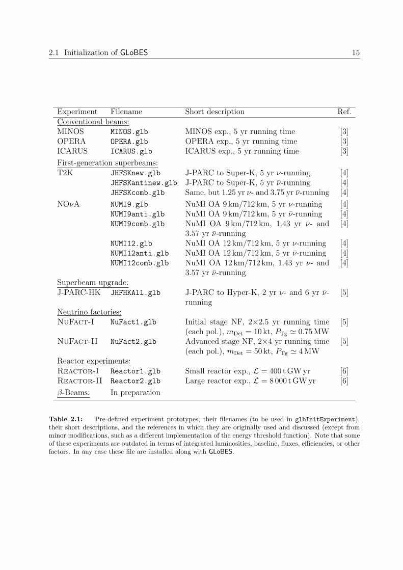
We will in this part not go into details of the experiment definition. The pre-definedexperiment prototypes in the data subdirectory are summarized in Table 2.1. They cor-respond (except from minor modifications) to the experiments in the respective referencesin the table. These files are installed to the directory ${prefix}/share/globes whichusually defaults to /usr/local/share/globes. It is useful to add this path to the valueof GLB_PATH.
2.1 Initialization of GLoBES
Before one can use GLoBES, one has to initialize the GLoBES library :
Function 2.1 void glbInit(char *name) initializes the library libglobes and has tobe called in the beginning of each GLoBES program. It takes the name name of the programas a string to initialize the error handling functions. In many cases, it is sufficient to usethe first argument from the command line as the program name (such as in example onpage 14).
1The data files (AEDL and supporting files) needed by the examples are already in place.
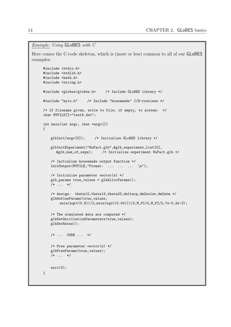
14 CHAPTER 2. GLoBES basics
Example: Using GLoBES with C
Here comes the C-code skeleton, which is (more or less) common to all of our GLoBESexamples:
#include <stdio.h>#include <stdlib.h>#include <math.h>#include <string.h>
#include <globes/globes.h> /* Include GLoBES library */
#include "myio.h" /* Include "housemade" I/O-routines */
/* If filename given, write to file; if empty, to screen: */char MYFILE[]="testX.dat";
int main(int argc, char *argv[]){
glbInit(argv[0]); /* Initialize GLoBES library */
glbInitExperiment("NuFact.glb",&glb_experiment_list[0],&glb_num_of_exps); /* Initialize experiment NuFact.glb */
/* Initialize housemade output function */InitOutput(MYFILE,"Format: ... ... ... \n");
/* Initialize parameter vector(s) */glb_params true_values = glbAllocParams();/* ... */
/* Assign: theta12,theta13,theta23,deltacp,dm2solar,dm2atm */glbDefineParams(true_values,
asin(sqrt(0.8))/2,asin(sqrt(0.001))/2,M_PI/4,M_PI/2,7e-5,2e-3);
/* The simulated data are computed */glbSetOscillationParameters(true_values);glbSetRates();
/* ... CODE ... */
/* Free parameter vector(s) */glbFreeParams(true_values);/* ... */
exit(0);
}
2.1 Initialization of GLoBES 15
Experiment Filename Short description Ref.Conventional beams:MINOS MINOS.glb MINOS exp., 5 yr running time [3]OPERA OPERA.glb OPERA exp., 5 yr running time [3]ICARUS ICARUS.glb ICARUS exp., 5 yr running time [3]
First-generation superbeams:T2K JHFSKnew.glb J-PARC to Super-K, 5 yr ν-running [4]
JHFSKantinew.glb J-PARC to Super-K, 5 yr ν-running [4]JHFSKcomb.glb Same, but 1.25 yr ν- and 3.75 yr ν-running [4]
NOνA NUMI9.glb NuMI OA 9 km/712 km, 5 yr ν-running [4]NUMI9anti.glb NuMI OA 9 km/712 km, 5 yr ν-running [4]NUMI9comb.glb NuMI OA 9 km/712 km, 1.43 yr ν- and
3.57 yr ν-running[4]
NUMI12.glb NuMI OA 12 km/712 km, 5 yr ν-running [4]NUMI12anti.glb NuMI OA 12 km/712 km, 5 yr ν-running [4]NUMI12comb.glb NuMI OA 12 km/712 km, 1.43 yr ν- and
3.57 yr ν-running[4]
Superbeam upgrade:J-PARC-HK JHFHKAll.glb J-PARC to Hyper-K, 2 yr ν- and 6 yr ν-
running[5]
Neutrino factories:NuFact-I NuFact1.glb Initial stage NF, 2×2.5 yr running time
(each pol.), mDet = 10 kt, PTg ' 0.75 MW[5]
NuFact-II NuFact2.glb Advanced stage NF, 2×4 yr running time(each pol.), mDet = 50 kt, PTg ' 4 MW
[5]
Reactor experiments:Reactor-I Reactor1.glb Small reactor exp., L = 400 t GW yr [6]Reactor-II Reactor2.glb Large reactor exp., L = 8 000 t GW yr [6]
β-Beams: In preparation
Table 2.1: Pre-defined experiment prototypes, their filenames (to be used in glbInitExperiment),their short descriptions, and the references in which they are originally used and discussed (except fromminor modifications, such as a different implementation of the energy threshold function). Note that someof these experiments are outdated in terms of integrated luminosities, baseline, fluxes, efficiencies, or otherfactors. In any case these file are installed along with GLoBES.

16 CHAPTER 2. GLoBES basics
In principle, the GLoBES user interface can currently handle up to 32 of different long-baseline experiments simultaneously, where the number of existing experiment definitionfiles can, of course, be unlimited. This means that their ∆χ2-values are added after theminimization over the systematics parameters, and before any minimization over the os-cillation parameters. Note that each experiment assumes a specific matter density profile,which means that it makes sense to simulate different operation modes within one exper-iment definition, and physically different baselines in different definitions. For details ofthe rate computation and simulation techniques, we refer at this place to Part II. Thoughthe simplest case of simulating one experiment may be most often used, using more thanone experiments are useful in many cases. For example, combinations of experiments canbe tested for complementarity and competitiveness by equal means within one program.In general, many GLoBES functions take the experiment number as a parameter, whichruns from 0 to glb_num_of_exps-1 in the order of their initialization in the program.2 Inaddition, using the parameter value GLB_ALL as experiment number initiates a combinedanalysis of all loaded experiments.
In general GLB_ALL can be used in many cases where there is an argument selecting‘i out of N ’, e.g. the 1st experiment out of 5, or the 5th rule of 20. In those cases usingGLB_ALL is equivalent to calling the corresponding function for all i in N and ‘add’ theeffect of each invocation, like in
for (i=0;i<N;i++) result += some_function(i);
is the same asresult = some_function(GLB_ALL);
Here the meaning of ‘add’ is, that whatever the desired result of calling some_function
is, this result is obtained for each i in N , e.g. setting the baseline in all experiments to acertain value or or compute the χ2 for each experiment and return the total result. Thereare however some functions where the action performed or the result is so complex that isnot possible or sensible to perform this for all i in N . Calling these functions with GLB_ALL
as argument will in any case result in an exit status indicating failure and the function willproduce an error message3.
For storing the experiments, GLoBES uses the initially empty list of experimentsglb_experiment_list. To add a pre-defined experiment to this list, one can use thefunction glbInitExperiment:
Function 2.2 int glbInitExperiment(char *inf, glb_exp *in, int *counter)
adds a single experiment with the filename inf to the list of currently loaded experiments.The counter is a pointer to the variable containing the number of experiments, and theexperiment in points to the beginning of the experiment list. The function returns zero ifit was successful.
Normally, a typical call of glbInitExperiment is
2Note that the global variable glb_num_of_exps must not be modified by the user.3if the verbosity level is set accordingly

2.1 Initialization of GLoBES 17
Quantities Examples UnitsAngles θ13, θ12, θ23, δCP RadiansMass squared differences ∆m2
21, ∆m231 eV2
Matter densities ρi g/cm3
Baseline lengths Li kmEnergies Eν GeVFiducial masses mDet t (reactor exp.) or kt (accelerator exp.),
depends on experiment definitionTime intervals trun yrSource powers PSource Useful parent particle decays/yr
(Neutrino factory, β-Beam),GW thermal power (reactor exps.),or MW target power (superbeams);depends on flux definition
Cross sections/E σCC/E 10−38 cm2/GeV2
Table 2.2: Quantities used in GLoBES, examples of these quantities, and their standard units in theapplication software.
glbInitExperiment("NuFact.glb",&glb_experiment_list[0],
&glb_num_of_exps);
In this case, the experiment in the file NuFact.glb is added to the internal global listof experiments, and the experiment counter is increased. The experiment then has thenumber glb_num_of_exps-1. The elements of the experiment list have the type glb_exp,which the user will not need to access directly in most cases. The experiment definitionfiles, which usually end with .glb, and any supporting files, are first of all searched in thecurrent directory, and then in the path given in the environment variable GLB_PATH.
A list of pre-defined experiment prototypes, their filenames, their short descriptions,and the references of their definitions can be found in Table 2.1. If the program cannotfind these files, or some of them are syntactically not correct, it will break at this place.
One can also remove all experiments from the evaluation list at running time:
Function 2.3 void glbClearExperimentList() removes all experiments from the inter-nal list and resets all counters.
Note that changing the number of experiments requires a new initialization of all parame-ters of the types glb_params and glb_projection if the number of experiments changes,since these parameter structures internally carry lists for the matter densities of all experi-ments. Similarly, once should never call glbAlloc... before the experiment initialization.

18 CHAPTER 2. GLoBES basics
2.2 Units in GLoBES and the integrated luminosity
While interacting with the user interface of GLoBES, parameters are transferred to and fromthe GLoBES library. In GLoBES, one set of units for each type of quantity is used in orderto avoid confusion about the definition of individual parameters. Table 2.2 summarizesthe units of the most important quantities. In principle, the event rates are proportionalto the product of source power × target mass × running time, which we call “integratedluminosity”. Since especially the definition of the source power depends on the experimenttype, the quantities of the three luminosity components are not unique and depend on theexperiment definition. Usually, one uses detector masses in kilotons for beam experiments,and detector masses in tons for reactor experiments. Running times are normally givenin years, where it is often assumed that the experiment runs 100% of the year. Thus, forshorter running periods, the running times need to be renormalized. Source powers areusually useful parent particle decays per year (neutrino factories, β-beams), target powerin mega watts (superbeams), or thermal reactor power in giga watts (reactor experiments).Since the pre-defined experiments in Table 2.1 are given for specific luminosities, it is usefulto read out and change these parameters of the individual experiments:
Function 2.4 void glbSetSourcePower(int exp, int fluxno, double power) setsthe source power of experiment number exp and flux number fluxno to power. The defi-nition of the source power depends on the experiment type as described above.
Function 2.5 double glbGetSourcePower(int exp, int fluxno) returns the sourcepower of experiment number exp and flux number fluxno.
Function 2.6 void glbSetRunningTime(int exp, int fluxno, double time) setsthe running time of experiment number exp and flux number fluxno to time years.
Function 2.7 double glbGetRunningTime(int exp, int fluxno) returns the runningtime of experiment number exp and flux number fluxno.
Function 2.8 void glbSetTargetMass(int exp, double mass) sets the fiducial detec-tor mass of experiment number exp to mass tons or kilotons (depending on the experimentdefinition).
Function 2.9 double glbGetTargetMass(int exp) returns the fiducial detector mass ofexperiment number exp.
Thus, these functions also demonstrate how to use the assigned experiment number andothers. These numbers run from 0 to the number of experiments-1, fluxes-1, etc., where theindividual elements are numbered in the order of their appearance. Note that the sourcepower and running time are quantities defined together with the neutrino flux, whereas thetarget mass scales the whole experiment. Thus, if one has, for instance, a neutrino and anantineutrino running mode, one can scale them independently.

2.3 Handling oscillation parameter vectors 19
2.3 Handling oscillation parameter vectors
Before we can set the simulated event rates or access any oscillation parameters, we needto become familiar with the concept GLoBES uses for oscillation parameters. In order totransfer sets of oscillation parameter vectors (θ12, θ13, θ23, δCP, ∆m2
21, ∆m231), the parameter
type glb_params is used. In general, this type is often transferred to and from GLoBESfunctions. Therefore, the memory for these vectors has to be reserved (allocated) beforethey can be used, and it has to be returned (freed) afterwards. GLoBES functions usuallyuse the pointers of the type glb_params for the input or output to the functions. As aninput parameter, the pointer has to be created and point towards a valid parameter struc-ture, where the oscillation parameters are read from. As an output parameter, the pointerhas to be created, too, and point towards a structure which will contain the return valueswill be written to. This parameter transfer concept seems to be very sophisticated, but, aswe will see in the next chapters, it hides a lot of complicated parameter mappings whichotherwise need to be done by the user. For example, not only the oscillation parametersare stored in the pointer structure, but also information on the matter densities of all of theinitialized experiments. Since GLoBES treats the matter density as a free parameter knownwith some external precision to include matter density uncertainties, the minimizers alsouse fit values and external errors for the matter densities of all loaded experiments. Moreprecisely, the matter density profile of each experiment i is multiplied by a scaling factorρi, which is stored in the density information of glb_params. Each of these scaling factorshas 1.0 as pre-defined value. Since it is in most cases not necessary to change this value, theuser does not need to take care of it. For a constant matter density, it is simply the ratio ofthe matter density and the average matter density specified in the experiment definition,i.e., ρi ≡ ρi/ρi. For a matter density profile, it acts as an overall normalization factor: Thematter density in each layer is multiplied by this factor. In most cases one wants to takea scaling factor of 1.0 here, which simply means taking the matter density profile as it isgiven in the experiment definition. For the treatment of correlations, however, an externalprecision of the scaling factor might be used to include the correlations with the matterdensity uncertainty. Note that the glb_params structures must not be initialized beforeall experiments are loaded, since the number of matter densities can only be determinedafter the experiments are initialized. Similarly, any change in the number of experimentsrequires that the parameter structures be re-initialized, i.e., freed and allocated again.
Note: Inverting the mass hierarchy is not precisely the same than to change from∆m2
31 → −∆m231. In this case the absolute value of ∆m2
32 changes also, which introducesa new frequency to the problem. Therefore, if we assume normal hierarchy whenever∆m2
31 > 0, the corresponding point in parameters space for inverted hierarchy is givenby ∆m2
31 → −∆m231 + ∆m2
21, because with this defintion the absolute value of ∆m232 is
unchanged and no new frequency is introduced.
Another piece of information will be returned from the minimizers (cf., Chapter 4)and transferred into the glb_params structure is the number of iterations used for the

20 CHAPTER 2. GLoBES basics
minimization, which is proportional to the running time of the minimizer. In general, theuser does not need to access the elements in glb_params directly. A number of functionsis provided to handle these parameter structures:
Function 2.10 glb_params glbAllocParams() allocates the memory space needed for aparameter vector and returns a pointer to it.
Function 2.11 void glbFreeParams(glb_params stale) frees the memory needed fora parameter vector stale and sets the pointer to NULL.
Function 2.12 glb_params glbDefineParams(glb_params in, double theta12,
double theta13,double theta23, double delta, double dms, double dma) assignsthe complete set of oscillation parameters to the vector in, which has to be allocated before.The return value is the pointer to in if the assignment was successful, and NULL otherwise.
Function 2.13 glb_params glbCopyParams(const glb_params source, glb_params
dest) copies the vector source to the vector destination. The return value is NULL ifthe assignment was not successful.
Function 2.14 void glbPrintParams(FILE *stream, const glb_params in) printsthe parameters in in to the file stream. The oscillation parameters, all density values,and the number of iterations are printed as pretty output. Use stdout for stream if youwant to print to the screen.
In addition to these basic functions, there are functions to access the individual parameterswithin the parameter vectors:
Function 2.15 glb_params glbSetOscParams(glb_params in, double osc, int
which) sets the oscillation parameter which in the structure in to the value osc. If theassignment was unsuccessful, the function returns NULL.
Function 2.16 double glbGetOscParams(glb_params in, int which) returns thevalue of the oscillation parameter which in the structure in.
In both of these functions, the parameter which runs from 0 to 5, where the parameters inGLoBES always have the order θ12, θ13, θ23, δCP, ∆m2
21, ∆m231. Alternatively to the number,
the constants GLB_THETA_12, GLB_THETA_13, GLB_THETA_23, GLB_DELTA_CP, GLB_DM_SOL,or GLB_DM_ATM can be used.
Similarly, the density parameters or number of iterations (returned by the minimizers)can be accessed:
Function 2.17 glb_params glbSetDensityParams(glb_params in, double dens,
int which) sets the density parameter which in the structure in to the value dens. If theassignment was unsuccessful, the function returns NULL. If GLB_ALL is used for which, thedensity parameters of all experiments will be set accordingly.

2.4 Computing the simulated data 21
Function 2.18 double glbGetDensityParams(glb_params in, int which) returnsthe value of the density parameter which in the structure in.
Function 2.19 glb_params glbSetIteration(glb_params in, int iter) sets thenumber of iterations in the structure in to the value iter. If the assignment wasunsuccessful, the function returns NULL.
Function 2.20 int glbGetIteration(glb_params in) returns the value of the numberof iterations in the structure in.
In total, the parameter vector handling in a program normally has the following order:
glbInitExperiment(...);
/* ... more initializations ... */
glb_params vector1 = glbAllocParams();
/* ... more vectors allocated ... */
/* Program code: assign and use vectors */
glbFreeParams(vector1);
/* ... more vectors freed ... */
/* ... end of program or glbClearExperimentList ... */
2.4 Computing the simulated data
Compared to existing experiments, which use real data, future experiments use simulateddata. Thus, the true parameter values and their results in form of the reference event ratevectors are simulated. After setting the true parameter values, the fit parameter valuescan be varied in order to obtain information on the measurement performance for thegiven set of true parameter values. Therefore, it is often useful to show the results of afuture measurement as function of the true parameter values for which the reference ratevectors are computed – at least within the currently allowed ranges. The true parame-ter values for the vacuum neutrino oscillation parameters have to be set by the functionglbSetOscillationParameters and the reference rate vector, i.e. the data, has to becomputed by a call to glbSetRates. This has to be done before any evaluation function isused and after the experiments have been initialized and also the experiment parametershave been adjusted which could change the rates (such as baseline or target mass). Thismeans that after any change of an experiment parameter, glbSetRates has to be called.Matter effects are automatically included as specified in the experiment definition. Wehave the following functions to assign and read out the vacuum oscillation parameters:

22 CHAPTER 2. GLoBES basics
Function 2.21 int glbSetOscillationParameters(const glb_params in) sets thevacuum oscillation parameters to the ones in the vector in.
Function 2.22 int glbGetOscillationParameters(glb_params out) returns the vac-uum oscillation parameters in the vector out. The result of the function is 0 if the call wassuccessful.
The reference rate vector is then computed with:
Function 2.23 void glbSetRates() computes the reference rate vector for the neutrinooscillation parameters set by glbSetOscillationParameters.
A complete example for a minimal GLoBES program can be found on Page 14.
2.5 Version control
In order to keep track of the used version of GLoBES, the software provides a number offunctions to check the GLoBES and experiment versions. It is up to the user to implementmechanisms into the program and AEDL files to check whether
• The program should only run with this specific version of GLoBES
• The program can only run with a minimum version of GLoBES
• The program can only run up to a certain GLoBES version.
The same holds for AEDL files: For example, some features may not be supported by earlierversions of GLoBES anymore. The program can then check the version of the AEDL fileand break if it is too old.
The functions in GLoBES for version control are:
Function 2.24 int glbTestReleaseVersion(const char *version) returns 0 if theversion string of the format “X.Y.Z” is exactly the used GLoBES version, 1 if it is older,and −1 if it is newer.
Function 2.25 int glbTestLibraryVersion(const char *version) returns 0 if theversion string of the format “X.Y.Z” is exactly the used GLoBES version, 1 if it is older,and −1 if it is newer. Note that the library and GLoBES versions are not the same.
Function 2.26 const char* glbVersionOfExperiment(int experiment) returns theversion string of the experiment number experiment. The version string is allocated withinthe experiment structure, which means that it cannot be altered and must not be freed bythe user.

23
Chapter 3
Calculating χ2 with systematics only
Calculating a χ2-value with or without systematics, but no correlations and degeneracies,is the simplest and fastest possibility to obtain high-level information on an experiment. Ingeneral, GLoBES uses the six independent oscillation parameters θ12, θ13, θ23, δCP, ∆m2
21,∆m2
31, as well as the matter density scaling factor ρ of each experiment. Thus, there are sixplus the number of experiments parameters determining the rate vectors. Using the matterdensity scaling factors in addition to the oscillation parameters will allow the simulationof the correlations with matter density uncertainties: In this approach, the matter densityprofile normalization ρ can be treated as parameter to be measured by the experiment,where an external precision given by observations is imposed (typically up to 5%). Forthis section, it is important to keep in mind that there are more parameters than just theoscillation parameters determining the simple χ2. However, as we have described in the lastsection, the mechanism for the matter density scaling factors is hidden in the definition ofglb_params: Each of the scaling factors is initially set to 1.0. Therefore, for the calculationof χ2 with systematics only, we do not have to care about the matter density scaling factors.
Keeping all oscillation parameters and matter density scaling factors fixed, one can usethe following functions to obtain the total χ2 of all specified oscillation channels includingsystematics:
Function 3.1 double glbChiSys(const glb_params in,int exp, int rule) returnsthe χ2 for the (fixed) oscillation parameters in, the experiment number exp, and the rulenumber rule. For all experiments or rules, use GLB_ALL as parameter value.
Note that the result of glbChiSys for all experiments or rules corresponds to the sum ofall of the individual glbChiSys calls. This equality will not hold for the minimizers in thenext sections anymore. An example how to use glbChiSys can be found on page 24.
The treatment of systematics in GLoBES is performed by the so-call pull method withthe help of auxiliary systematics parameters. They are taken completely uncorrelatedamong different rules, and treated with simple Gaußian statistics. In general, a rule is aset of signal and background event rates coming from different oscillation channels, wherethe event rates of all rule contributions are added. For more details of the rule concept,see Part II of this manual, and for the treatment of systematics, see Sec. 9.6.

24 CHAPTER 3. Calculating χ2 with systematics only
Example: Correlation between sin2 2θ13 and δCP
A typical and fast application for glbChiSys is the visualization of two-parametercorrelations using systematics only. For example, to calculate the two-parameter cor-relation between sin2 2θ13 and δCP at a neutrino factory, one can use the following codeexcerpt from example1.c:
/* Initialize parameter vector(s) and compute simulated data */
glbDefineParams(true_values,theta12,theta13,theta23,deltacp,sdm,ldm);
glbDefineParams(test_values,theta12,theta13,theta23,deltacp,sdm,ldm);
glbSetOscillationParameters(true_values); glbSetRates();
/* Iteration over all values to be computed */
double x,y,res;
for(x=-4.0;x<-2.0+0.01;x=x+2.0/50)
for(y=0.0;y<200.0+0.01;y=y+200.0/50)
{
/* Set parameters in vector of test values */
glbSetOscParams(test_values,asin(sqrt(pow(10,x)))/2,GLB_THETA_13);
glbSetOscParams(test_values,y*M_PI/180.0,GLB_DELTA_CP);
/* Compute Chi2 for all loaded experiments and all rules */
res=glbChiSys(test_values,GLB_ALL,GLB_ALL);
AddToOutput(x,y,res);
}
The resulting data can then be plotted as a contour plot (2 d.o.f.):
10� 4 10
� 3 10� 2
sin2 2�
13
0
50
100
150
200
� CP
Deg
rees
1�2�3�

CHAPTER 3. Calculating χ2 with systematics only 25
One example for a systematics parameter the signal normalization error, i.e., an errorto the overall normalization of the signal. For illustration, we assume that the signal eventrate in the ith bin s0
i of one oscillation channel is altered by the overall normalizationauxiliary parameter of this channel, i.e.,
si = si(ns) = s0i · (1 + ns), (3.1)
where ns is the signal normalization parameter. The total number of events in the ith binxi also includes the background event rates bi, i.e., xi = si + bi, which may have theirown systematics parameters. In order to implement an overall signal normalization errorσns , the χ2, which includes all event rates xi of all bins, is minimized over the auxiliaryparameter ns:
χ2 = minns
(χ2(ns, . . .) +
(ns)2
σ2ns
). (3.2)
This minimization is done independently for all auxiliary parameters of the rule. The totalχ2 for the considered experiment is finally obtained by repeating this procedure for allrules and adding their χ2-values. In general, the situation is more complicated because ofthe usage of many systematical errors. More details about systematics parameters and thedefinition of signal, background, and oscillation channels can be found in Sec. 9.6, too.
The systematics minimization of an experiment can be easily switched on and off withglbSwitchSystematics, i.e., one can also compute the χ2 with statistics only. In addition,several options for systematics are available, such as only using total event rates withoutspectral information. For details, we refer to Chapter 7.

26 CHAPTER 3. Calculating χ2 with systematics only

27
Chapter 4
Calculating χ2-projections: how onecan include correlations
This chapter deals with the rather complicated issue of n-parameter correlations. It isone of the greatest strengths of this software to include the full n-parameter correlationin the high-dimensional parameter space with reasonable effort. Of course, calculating χ2-projections is somewhat more complicated than using systematics only. Therefore, we usea simple step by step introduction to the problem.
4.1 Introduction
In principle, the precision of an individual parameter measurement including correlationsin the χ2-approach can be obtained as the projection of the n-dimensional fit manifold ontothe respective axis. Similarly, one can project the fit manifold onto a plane, such as thesin2 2θ13-δCP-plane, if one wants to show the allowed region in this plane with all the otherparameter correlations included. In practice, this projection is very difficult: a grid-basedmethod would need (Ngrid)
n function calls of glbChiSys to calculate the projection ontoone dimension including the full n-parameter correlation, where Ngrid is the number ofpoints in each direction of the lattice. For example, taking only Ngrid = 20 and n = 7 (sixoscillation parameters and matter density) would mean more than one billion function callsof glbChiSys. One can easily imagine that these would be too many for any reasonableapplication.
The solution to this problem is using a n-dimensional, local minimizer for the projectioninstead of a grid-based method, where we will illustrate this minimization process later.It turns out that such a minimizer can include a full 6-parameter correlation with of theorder of 1 000 function calls of glbChiSys. For the minimization we use a derivative freemethod due to Powell in a modified [7] version1.
1Not needing derivatives is highly desired since the event rate depends in a non-linear way on theoscillation parameters, thus there is no easy analytical way to obtain derivatives of the χ2 function.

28 CHAPTER 4. Calculating χ2-projections: how one can include correlations
Thus, for each point on the projection axis/plane, one can obtain a result within about10 to 30 seconds on a modern computer, which means that the complete measurementprecision for one fixed true parameter set can be obtained in as much as 10 to 15 minutes.One can easily imagine that such a minimizer makes more sophisticated applications pos-sible with the help of overnight calculations, such as showing the dependencies on the trueparameter values.
This approach also has one major disadvantage: There is no such thing as a globalminimization algorithm or even an algorithm which guarantees to find all local minimaof a function. In practice this means using a local minimizer, one may end up in anunwanted local minimum and not in the investigated (possibly global) one or one maymiss a local minimum which affects the results2. The only way out of this dilemma is touse some heuristic approach, i.e. although one can not guarantee anything one can useschemes which work in most cases and announce their failure loudly. In order to use sucha heuristic some (analytical or numerical) knowledge on the topology of the fit manifoldis necessary. With this knowledge it is possible to obtain an approximate position foreach local minimum and thus to start the local minimizer close enough to the investigatedminimum. Fortunately, this can be done quite straightforward in most cases, since thestructure of the neutrino oscillation formulas does not cause very complicated topologies ofthe fit manifolds. Especially the simulation of reactor experiments and conventional beamsor superbeams is rather simple with purely numerical approaches. Neutrino factories have,especially for small values of θ13, a much more complicated topology. In this case, resultsof the many analytical discussions of this issue can be used. This means that one canimplicitly use the analytical knowledge to obtain better predictions for the location of aminimum. One can easily imagine that the used methods then also depend on the regionof the parameter space. In this manual, we only use examples with a neutrino factory,since some of these complications can be illustrated there. Albeit the methods describedhere are neither complete nor will they work everywhere in the parameter space. It is inany case up to the user to make sure that the results are what he/she thinks.
Some more words of warning with respect to results obtained by projecting the χ2: Theresults obtained this way are always only a upper bound on the value of the projected χ2
function, i.e. an undiscovered minimum decreases the value of the the projected χ2 function.If the value of the χ2 function in the missed minimum is larger than the previously foundones it will not influence the value of the projected value. Thus, one can only run thedanger to obtain a too optimistic solution if one does not find the other local minimaappearing below the chosen confidence level. Thus, with this approach and proper usage,it should not possible to produce a too pessimistic solution. However, if one is not carefulenough to locate all local minima, one can easily produce too optimistic solutions. Thisdanger can be summarized as follows:
Too pessimistic result < Real result︸ ︷︷ ︸Located by careful usage
≤ GLoBES result < Too optimisitic result
2NB – Implementing a grid-based method which guarantee to find all local minima is not straightforwardeither, to say the least.
4.2 The treatment of external input 29
In many cases, the fit manifold is restricted by the knowledge from earlier experiments.For example, the knowledge on the solar parameters will in most cases be supplied by thesolar neutrino experiments. If the external precision of a parameter is at the time of themeasurement better than the one of the experiment itself, one usually will use this external,better knowledge and impose a corresponding constraint on this parameter. This externalknowledge may reduce the extension of the n-dimensional fit manifold in the respectivedirection. In the most extreme case, keeping all parameters but the measured one fixed inthe analysis is equivalent to the assumption that all parameters are determined externallywith infinitively high precisions. As this is a quite strong assumption, one should alwayscheck the consequences of relaxing it and using realistic errors. Only if such a test hasdemonstrated that the impact of the uncertainty on a given fit parameter is negligible itcan be assumed as fixed safely. The inclusion of external input in GLoBES is done bythe use of Gaußian priors: We assume that an external measurement has determined themeasured parameter to be at the central value (which we call starting value) with a 1σGaußian error (which we call input error). The explicit definition of these priors will beshown in the next section.
4.2 The treatment of external input
It is one of the strengths of the GLoBES software to use external input in order to reducethe extension of the fit manifold with the knowledge from external (earlier) measurements.The treatment of external input is done by the addition of Gaußian so-called priors to thesystematics-minimized χ2-function. For example, for the matter density, one obtains asthe final projected χ2
F after minimization over the matter density scaling factor ρ
χ2F = min
ρ
(χ2(ρ) +
(ρ− ρ0)2
σ2ρ
). (4.1)
This example is a very simple one, since in fact the minimization is simultaneously per-formed over all priors and free oscillation parameters. In Eq. (4.1), ρ0 is the starting valueof the prior, and σρ the 1σ absolute (half width) input error. Thus, it is assumed that anexternal measurement has determined the matter density with a precision (input error) σρ
at the central value ρ0. Usually, the starting value is fixed at the best-fit value, and theinput error to the 1σ half width of the external measurement. For the matter density, ρ0
is usually set to 1.0 corresponding to the actual matter density profile such as given by theexperiment definition file, and σρ to the relative matter density uncertainty (e.g., 0.05 for5% uncertainty).
In principle, one can set the priors for the matter density and all oscillation parameters.For example, if the disappearance channels of the experiment determine the leading oscil-lation parameters with unprecedented precisions, one can omit the respective input errors.In GLoBES, a value of 0 corresponds3 to neglecting the prior. If, however, earlier external
3to be precise, a value for the error in between −10−12 and +10−12

30 CHAPTER 4. Calculating χ2-projections: how one can include correlations
measurements provide better information, one can set their absolute precisions with theinput errors. The starting values are usually chosen to be the best-fit values of this exter-nal experiments, such as for the input from solar experiments. In some cases, it may benecessary to adjust them, such as for artificial constraints to the oscillation parameters. Inother cases, minor modifications of the starting values can cause a faster convergence ofthe algorithm. For example, for the investigation of the opposite-sign solution, one can usethe prior to constrain ∆m2
31 in order to force the minimizer not to fall into the (unwanted)true-sign solution. In this case, the starting value of ∆m2
31 would be set to ρ0∆m2
31= −∆m2
31,
and a σ∆m231
of the order of ∆m231 would be imposed. For the algorithm, it would then be
rather difficult to converge into the unwanted true-sign solution. However, note that oneshould in this case check that the actually determined value for ∆m2
31 after minimizationis close enough to the guessed value −∆m2
31 in order to avoid significant artifical contribu-tions of the priors to the final χ2. Alternatively one could re-run the minimizer with theposition of the previously found minimum as starting position but now with switching offthe constraint on ∆m2
31.In order to set the starting values and input errors, two function have to be called before
the usage of any minimizer:
Function 4.1 int glbSetStartingValues(const glb_params in) sets the starting val-ues for all of the following minimizer calls to in.
Function 4.2 int glbSetInputErrors(const glb_params in) sets the input errors forall of the following minimizer calls to in. An input error of 0 corresponds to not takinginto account the respective prior.
Accordingly, there are functions to return the actually set starting values and input errors:
Function 4.3 int glbGetStartingValues(glb_params out) writes the currently setstarting values to out.
Function 4.4 int glbGetInputErrors(glb_params out) writes the currently set inputerrors to out.
All functions take or return as many matter density parameters as there are initializedexperiments. In addition, they return −1 if the operation was not successful.
Eventually, a typical initialization of the external input with 10% external precisionsfor the solar parameters4, and 5% matter density uncertainties for all experiments lookslike this:
glbDefineParams(input_errors,theta12*0.1,0,0,0,sdm*0.1,0);
glbSetDensityParams(input_errors,0.05,GLB_ALL);
glbSetStartingValues(true_values);
glbSetInputErrors(input_errors);
4In fact, accelerator-based long-baseline experiments are primarily sensitive to the product sin 2θ12 ·∆m2
21, which means that these errors effectively add up to an error of this product of about 15%.
4.3 Projection onto the sin2 2θ13-axis or δCP-axis 31
In this example, the starting values are set to the true (simulated) values. Remember thatinitially the matter density scaling factors are all 1.0, which means that they do not needto be adjusted for the starting values.
Though the priors are an elegant way to treat external input, there are also somecomplications with priors. The following hints are for the more advanced GLoBES user:
1. The priors are only added once to the final χ2, no matter how many experimentsthere are simulated. This is already one reason (besides the minimization) why thesum of all projected χ2’s of the individual experiments cannot correspond to the χ2
of the combination of all experiments.
2. Priors are not used for parameters which are not minimized over, i.e., kept fixed.This will be important together with arbitrary projections using glbChiNP. A moresubtile consequence is the comparison of fit manifold sections and projections for thesolutions where the absolute minimum χ2 is larger than zero, i.e., degeneracies otherthan the true solution. In this case, the sections and projections are not comparable ifnot corrected by the prior contributions, where the correction can be obtained as theχ2-difference at the minimum. For example, projecting the sgn(∆m2
31)-degeneracyonto the θ13-δCP-plane and comparing it with the section (all other parameters fixed),the section region would in many cases be larger than the projection region if thepriors are not added to the section. At the true solution, this problem usually doesnot occur because the prior contributions are close to zero.
3. Currently, GLoBES only supports Gaußian priors for the individual oscillation pa-rameters. Especially for the solar parameters, this is only an approximation, sincethey are imposed on θ12 and not on sin 2θ12, sin 2θ12 ·∆m2
21, or sin θ12. Later versionsof GLoBES may include more alternatives.
4.3 Projection onto the sin2 2θ13- or δCP-axis
The projection onto the sin2 2θ13- (or δCP-) axis is performed by fixing sin2 2θ13 (or δCP)and minimizing the χ2-function over all free fit parameters and the matter densities. Weillustrate this method at the example of the projection of the two-dimensional manifold inthe sin2 2θ13-δCP-plane onto the sin2 2θ13-axis in Fig. 4.1. In this figure, the left-hand plotshows the correlation in the sin2 2θ13-δCP-plane computed with glbChiSys. The right-handplot illustrates the projection of this two-dimensional manifold onto the sin2 2θ13 axis byminimizing χ2 over δCP. In this simple example, the minimization is done along the verticalgray lines in the left hand plot. The obtained minima are located on the thick gray curve,which means the the right-hand plot represents the χ2-value along this curve. In fact, onecan easily see that one obtains the correct projected 3σ errors in this example (cf., arrows).This figure illustrates the projection of a two-parameter correlation. In general, the fulln-parameter correlation is treated similarly by the simultaneous (local) minimization overall free fit parameters.

32 CHAPTER 4. Calculating χ2-projections: how one can include correlations
Example: Projection of two- and n-dimensional manifold onto sin2 2θ13-axis
This example demonstrates how to project the fit manifold onto the sin2 2θ13-axis, i.e.,how one can include correlations. We compute two sets of data: one for keeping all pa-rameters but δCP fixed (two-parameter correlation), and one for keeping all parametersfree (multi-parameter correlation). However, we impose external precisions for the solarparameters and the matter density. The following code excerpt is from example2.c:
/* Set starting values and input errors for all projections */
glbDefineParams(input_errors,theta12*0.1,0,0,0,sdm*0.1,0);
glbSetDensityParams(input_errors,0.05,GLB_ALL);
glbSetStartingValues(true_values);
glbSetInputErrors(input_errors);
/* Define my own two-parameter projection for glbChiNP: Only deltacp is free! */
glbDefineProjection(th13_projection,GLB_FIXED,GLB_FIXED,GLB_FIXED,GLB_FREE,GLB_FIXED,GLB_FIXED);
glbSetProjection(th13_projection);
/* Iteration over all values to be computed */
double x,res1,res2;
for(x=-4;x<-2.0+0.001;x=x+2.0/50)
{
/* Set fit value of stheta */
glbSetOscParams(test_values,asin(sqrt(pow(10,x)))/2,1);
/* Guess fit value for deltacp in order to safely find minimum */
glbSetOscParams(test_values,200.0/2*(x+4)*M_PI/180,3);
/* Compute Chi2 for user-defined two-parameter correlation */
res1=glbChiNP(test_values,NULL,GLB_ALL);
/* Compute Chi2 for full correlation: minimize over all but theta13 */
res2=glbChiTheta(test_values,NULL,GLB_ALL);
AddToOutput(x,res1,res2);
}
The two lists of data then represent the sin2 2θ13 precisions with two-parameter corre-lations (gray-shaded) and multi-parameter correlations (arrows):
10� 4 10
� 3 10� 2
sin2 2�
13
0
5
10
15
20
� 2
1�
2�
3�
(Same parameters as on page 24 and in Fig. 4.1, but 1 d.o.f.)

4.3 Projection onto the sin2 2θ13-axis or δCP-axis 33
10� 4 10
� 3 10� 2
sin2 2�
13
0
50
100
150
200
� CP
Deg
rees
Correlation between sin22 � 13 and � CP
1�2�3�
10� 4 10
� 3 10� 2
sin2 2� 13
0
5
10
15
20
� 2
Projection onto sin22 � 13 axis
1
2
3
Figure 4.1: Left plot: The correlation between sin2 2θ13 and δCP as calculated in the example onpage 24, but for 1 d.o.f. only. Right plot: The χ2-value of the projection onto the sin2 2θ13-axis as functionof sin2 2θ13. The projection onto the sin2 2θ13-axis is obtained by finding the minimum χ2-value for eachfixed value of sin2 2θ13 in the left-hand plot, i.e., along the gray vertical lines. The thick gray curve marksthe position of these minima in the left-hand plot. The arrows mark the obtained fit ranges for sin2 2θ13
at the 3σ confidence level (1 d.o.f.), i.e., the precision of sin2 2θ13.
The following functions are some of the simplest minimizers provided by GLoBES:
Function 4.5 double glbChiTheta(const glb_params in, glb_params out, int
exp) returns the projected χ2 onto the θ13-axis for the experiment exp. For the simulationof all initialized experiments, use GLB_ALL for exp. The values in in are the guessed fitvalues for the minimizer (all parameters other than θ13) and the fixed fit value of θ13. Theactually determined parameters at the minimum are returned in out, where θ13 is still atits fixed value. If out is set to NULL, this information will not be returned.
Function 4.6 double glbChiDelta(const glb_params in, glb_params out, int
exp) returns the projected χ2 onto the δCP-axis for the experiment exp. For the simulationof all initialized experiments, use GLB_ALL for exp. The values in in are the guessed fitvalues for the minimizer (all parameters other than δCP) and the fixed fit value of δCP.The actually determined parameters at the minimum are returned in out, where δCP isstill at its fixed value. If out is set to NULL, this information will not be returned.
All of the minimization functions have a similar parameter structure: The fixed fitparameter value and the guessed starting point of the minimizer, i.e., the guessed positionof the minimum, are transferred in the list in. Part of this list are the matter densityscaling factors of all experiments, which are also minimized over. The minimizer is then

34 CHAPTER 4. Calculating χ2-projections: how one can include correlations
started at the guessed point and runs into the local minimum, where the fit parameterof the projection axis is fixed. For the true solution, it is usually sufficient to start theminimizer at the true parameter values. However, the convergence speed might be better bystarting it slightly off this point. In addition, there are problems in many cases with morecomplicated topologies, which means that better guesses for the position of the minimumare needed. The position of the minimum is then returned in out together with thenumber of iterations used for the minimization. It is very often useful to print the outputof the minimization with glbPrintParams in order to check that the minimum is theappropriate one. For example, if the minimizer ends up in the wrong-sign solution in∆m2
31, priors can be used to force it into the tested minimum. In addition, the numberof iterations used allows an optimization of the convergence speed. Note that before anyminimization, glbSetStartingValues and glbSetInputErrors have to be used at leastonce. In addition, note that the resulting χ2 of glbChiTheta (or glbChiDelta) for thecombination of more than one experiment is not equal to the sum of the individual χ2-values anymore. This has two reasons: First, the topology of the fit manifold is alteredby the addition of χ2-values of different experiments. Thus, after the minimization, theposition of the minimum can be different to the ones of the individual experiments. Second,the priors for the external knowledge on the parameters are only added once – independentof the number of experiments.
The output of the minimizer in out carries as many matter density scaling factorsas there are experiments. Either one (for the simulation of one experiment) or all (forthe simulation of all experiments) are different from 1.0 if matter density uncertainties arepresent, since each experiment may face other matter density conditions. The minimizers ofindividual experiments “know” which experiment they are currently treating, which meansthat they only returned the matter density scaling factor of the appropriate experiment.For example, calculating glbChiTheta for the last experiment number, the last densityvalue will be returned. This approach turns out to be extremely useful together with thesimulation of more than one experiment. One can, for instance, locate the degeneraciesof all individual experiments. In order to test if these degeneracies are still present inthe combination of all experiments (which has a very different topology), one can test thecombination of experiments with the output out from the individual experiments. In thiscase, even the correct matter density scaling factor output is used.
The example on page 32 demonstrates how one can obtain Fig. 4.1 (right) with keepingall parameters but δCP fixed, as well as how one can include the full n-parameter correlationwith external input. It also demonstrates how these two compare to each other. Onecan easily read off this example that there is a substantial impact of the correlation withoscillation parameters other than δCP. Note that it uses the function glbChiNP for arbitraryprojections from the next section for the minimization over δCP. In addition, there is oneinteresting feature in guessing the oscillation parameters in this example: In order to avoidfalling into the wrong minimum, the fit value of δCP is guessed from Fig. 4.1 (left). Thisquite sophisticated “guessing” is typical for neutrino factories because of the (δCP, θ13)-degeneracy, whereas it is for superbeams often sufficient to use the true values. A strongindication for a wrong guessing are discontinuous jumps in the projected χ2-function, where

4.4 Projection onto any hyperplane 35
the minimizer jumps from one minimum to another. In such cases, the starting point ofthe minimizer has to be adjusted to help it find the true minimum.
Other examples for projections onto a parameter axis while keeping exactly one param-eter fixed are glbChiTheta23, glbChiDm, and glbChiDms, which can be found in Table 1.1on page 4.
4.4 Projection onto any hyperplane
In general, one can show the measurement result in any k-dimensional hyperplane, wherek is smaller than the dimension of the parameter space n, and thus the dimension of thefit manifold. In this case, k parameters are fixed and n − k parameters are minimizedover. One such example is the projection of the fit manifold onto the sin2 2θ13-δCP-plane,i.e., k = 2 here. In this case, the two parameters sin2 2θ13 and δCP are kept fixed, and theothers are minimized over. The corresponding function is
Function 4.7 double glbChiThetaDelta(const glb_params in, glb_params out,
int exp) returns the projected χ2 onto the θ13-δCP-plane for the experiment exp. Forthe simulation of all initialized experiments, use GLB_ALL for exp. The values in in arethe guessed fit values for the minimizer (all parameters other than θ13 and δCP) and thefixed fit values of θ13 and δCP. The actually determined parameters at the minimum arereturned in out, where θ13 and δCP are still at their fixed values. If out is set to NULL,this information will not be returned.
This function works analogously to the ones in the last section. They can, for example, beused to obtain a figure similar to Fig. 4.1, left. The example on page 32 illustrates thenthe difference between the projections of the “eggs” within the sin2 2θ13-δCP-plane onto theθ13-axis. Though the running time for one call of these functions is somewhat shorter thanthe one for the sin2 2θ13- or δCP-projections, one has to compute a two-dimensional arrayfor such a figure (instead of a one-dimensional list). Therefore, the overall computationaleffort is much higher, i.e., in the order of hours. In many cases, it is therefore convenientto run glbChiSys first to obtain a picture of the manifold and to adjust the parameterranges. Then, one can run glbChiThetaDelta for a complete evaluation of the problemincluding correlations.
In principle, one can also use three- or more-dimensional projections. In addition, onemay want to use a different set of parameters for single- or two-parameter projections.The very flexible function glbChiNP is designed for this purpose. However, because of itsflexibility, it involves more sophistication.
In order to define arbitrary projections, we introduce the vector glb_projection, whichis very similar to the oscillation parameter vector glb_params. Normally, the user doesnot need to access this type directly: A set of function similar to the ones for glb_paramsis provided. The purpose of glb_projection is to tell GLoBES what parameters are fixed,and what are minimized over. Thus, in comparison to glb_params, it does not take valuesfor the parameters, but flags GLB_FIXED or GLB_FREE. For example, the projection onto
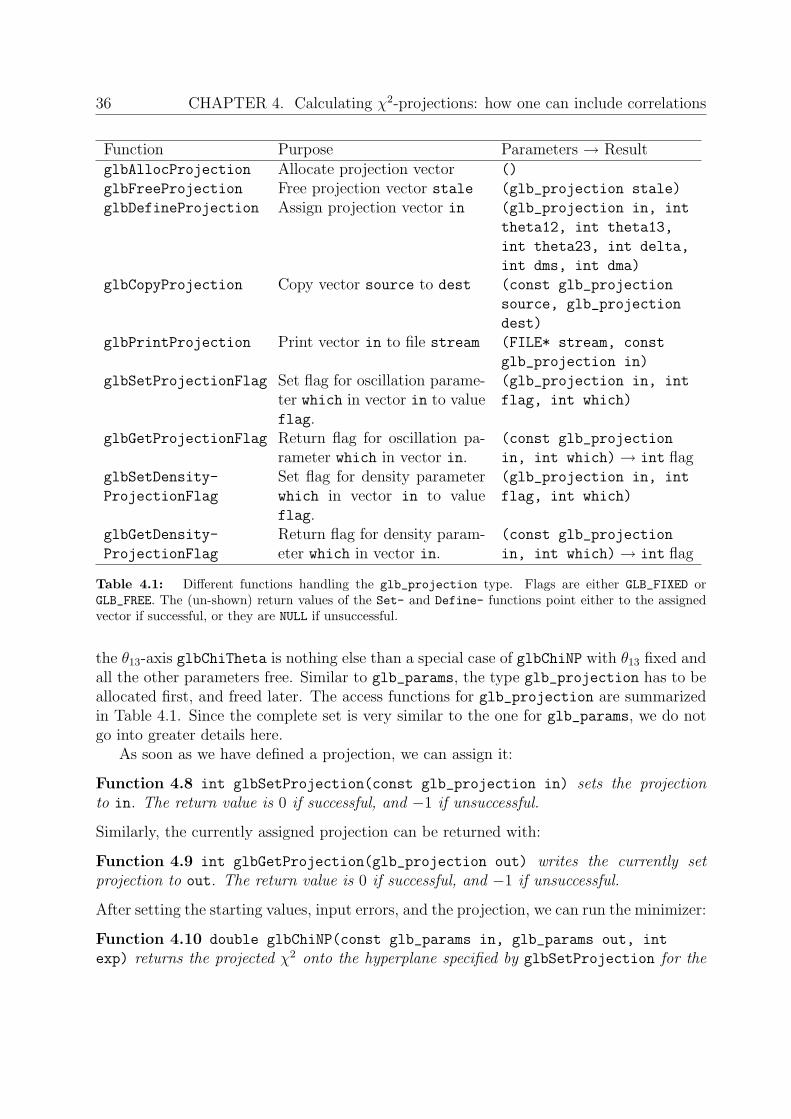
36 CHAPTER 4. Calculating χ2-projections: how one can include correlations
Function Purpose Parameters → ResultglbAllocProjection Allocate projection vector ()
glbFreeProjection Free projection vector stale (glb_projection stale)
glbDefineProjection Assign projection vector in (glb_projection in, int
theta12, int theta13,
int theta23, int delta,
int dms, int dma)
glbCopyProjection Copy vector source to dest (const glb_projection
source, glb_projection
dest)
glbPrintProjection Print vector in to file stream (FILE* stream, const
glb_projection in)
glbSetProjectionFlag Set flag for oscillation parame-ter which in vector in to valueflag.
(glb_projection in, int
flag, int which)
glbGetProjectionFlag Return flag for oscillation pa-rameter which in vector in.
(const glb_projection
in, int which)→ int flagglbSetDensity-
ProjectionFlag
Set flag for density parameterwhich in vector in to valueflag.
(glb_projection in, int
flag, int which)
glbGetDensity-
ProjectionFlag
Return flag for density param-eter which in vector in.
(const glb_projection
in, int which)→ int flag
Table 4.1: Different functions handling the glb_projection type. Flags are either GLB_FIXED orGLB_FREE. The (un-shown) return values of the Set- and Define- functions point either to the assignedvector if successful, or they are NULL if unsuccessful.
the θ13-axis glbChiTheta is nothing else than a special case of glbChiNP with θ13 fixed andall the other parameters free. Similar to glb_params, the type glb_projection has to beallocated first, and freed later. The access functions for glb_projection are summarizedin Table 4.1. Since the complete set is very similar to the one for glb_params, we do notgo into greater details here.
As soon as we have defined a projection, we can assign it:
Function 4.8 int glbSetProjection(const glb_projection in) sets the projectionto in. The return value is 0 if successful, and −1 if unsuccessful.
Similarly, the currently assigned projection can be returned with:
Function 4.9 int glbGetProjection(glb_projection out) writes the currently setprojection to out. The return value is 0 if successful, and −1 if unsuccessful.
After setting the starting values, input errors, and the projection, we can run the minimizer:
Function 4.10 double glbChiNP(const glb_params in, glb_params out, int
exp) returns the projected χ2 onto the hyperplane specified by glbSetProjection for the
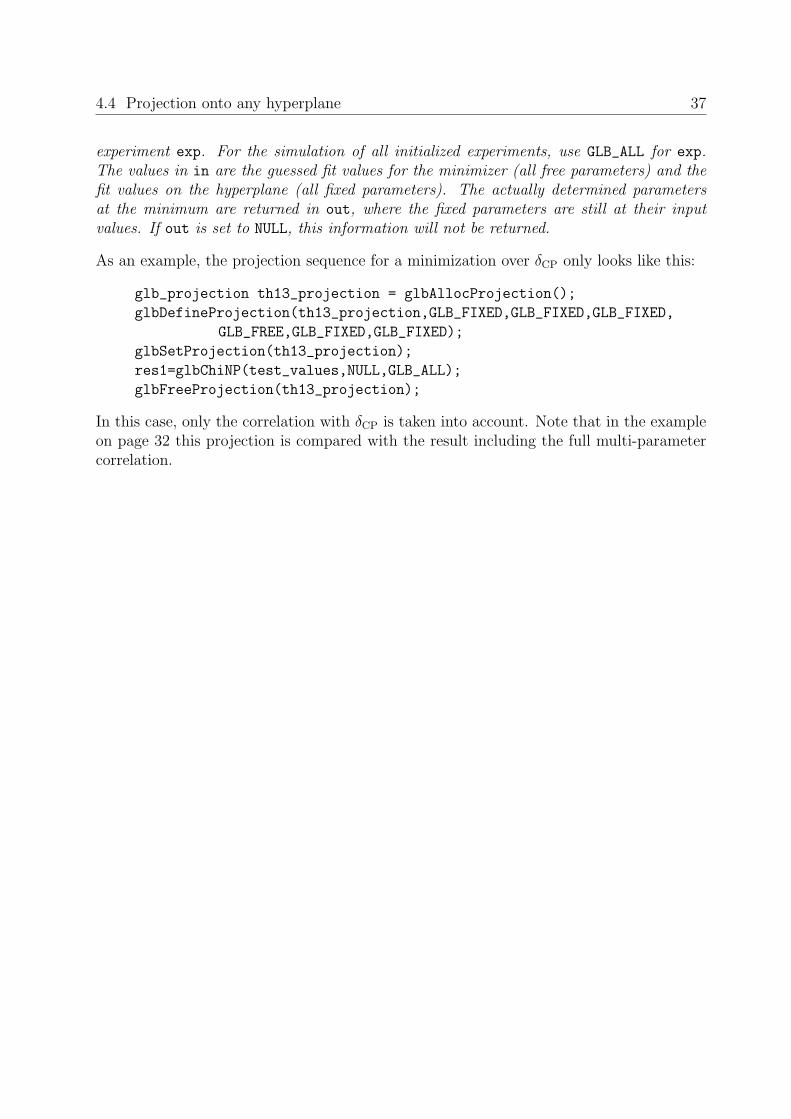
4.4 Projection onto any hyperplane 37
experiment exp. For the simulation of all initialized experiments, use GLB_ALL for exp.The values in in are the guessed fit values for the minimizer (all free parameters) and thefit values on the hyperplane (all fixed parameters). The actually determined parametersat the minimum are returned in out, where the fixed parameters are still at their inputvalues. If out is set to NULL, this information will not be returned.
As an example, the projection sequence for a minimization over δCP only looks like this:
glb_projection th13_projection = glbAllocProjection();
glbDefineProjection(th13_projection,GLB_FIXED,GLB_FIXED,GLB_FIXED,
GLB_FREE,GLB_FIXED,GLB_FIXED);
glbSetProjection(th13_projection);
res1=glbChiNP(test_values,NULL,GLB_ALL);
glbFreeProjection(th13_projection);
In this case, only the correlation with δCP is taken into account. Note that in the exampleon page 32 this projection is compared with the result including the full multi-parametercorrelation.

38 CHAPTER 4. Calculating χ2-projections: how one can include correlations
39
Chapter 5
Locating degenerate solutions
In the last chapter, we introduced the projection of any set of k parameters onto anyn−k dimensional hyperplane, which was performed by the minimization over the k free fitparameters. Similarly, one can minimize over all n parameters to find the local minimumclose to any starting point. This approach is very useful for the exact numerical location of adegeneracy if its approximate position is known. For the determination of the approximateposition, one can use analytical approaches or an educated guess. Though the usage ofthe all-parameter minimizers is quite simple, one should keep in mind that they are localminimizers. Therefore, one may need a very sophisticated application software to find alldegenerate solutions.
The function to perform the all-parameter minimization is glbChiAll:
Function 5.1 double glbChiAll(const glb_params in, glb_params out, int
exp) returns the minimized χ2 over all parameters for the experiment exp. For thesimulation of all initialized experiments, use GLB_ALL for exp. The values in in are theguessed fit values for the minimizer. The actually determined parameters at the minimumare returned in out. If out is set to NULL, this information will not be returned.
This function takes the suspected position of the local minimum and returns its actualposition in out, as well as the χ2-value at the minimum as return value. Thus, the returnvalue can be immediately used to judge whether the located degeneracy appears at thechosen confidence level.
The example on page 40 illustrates how to locate the sgn(∆m231)-degeneracy and show
the corresponding degenerate solution in the sin2 2θ13-δCP-plane together with the originalsolution. In this case, the position of the degeneracy can be easily guessed to be at the trueparameter values but with inverted1 ∆m2
31. The minimizer then runs off the plane of theseparameters into the local minimum. It is very important to take into account the positionof the degeneracy off this plane, since the actual χ2 in the minimum is probably lower thanin the plane. Thus, the degeneracy may not even appear at the chosen confidence levelin the plane, but it does appear at the real minimum. The two sections through the fit
1For a exact definition of inverted hierarchy, see page 19.

40 CHAPTER 5. Locating degenerate solutions
Example: Finding the sgn(∆m231)-degeneracy
In many cases, one can find the exact position of the sgn(∆m231)-degeneracy with
glbChiAll, where one starts the local minimizer at the suspected position and let it runinto the minimum. The following code excerpt corresponds to finding the degeneratesolution for the example on page 24, and it is from example3.c:
/* Set starting vales to suspected position at opposite sign of ldm */
glbDefineParams(starting_values,theta12,theta13,theta23,deltacp,sdm,-ldm);
/* Set input errors for external input, where some information on ldm
is imposed in order to avoid falling into the right-sign solution */
glbDefineParams(input_errors,theta12*0.1,0,0,0,sdm*0.1,ldm/3);
glbSetDensityParams(input_errors,0.05,GLB_ALL);
glbSetStartingValues(starting_values);
glbSetInputErrors(input_errors);
/* Localize degenerate solution by minimization over all parameters
*/
double CL=glbChiAll(starting_values,deg_pos,GLB_ALL);
/* Now: CL is the chi2 of the deg. solution and deg_pos the position */
Using ent_pos to obtain a section of the degeneracy in the sin2 2θ13-δCP-plane (cf.,example3.c), one can plot it as a contour plot in addition to the original solution (2d.o.f., gray curves):
10� 4 10
� 3 10� 2
sin2 2�
13
0
50
100
150
200
� CP
Deg
rees
1�2�3�

CHAPTER 5. Locating degenerate solutions 41
manifold shown in the figure on page 40 therefore do not appear at the same oscillationparameter values (except from the ones shown in the figure).2
For the more advanced reader, a number of tricks can be useful for the numericallocalization of degenerate solutions:
Minimum χ2 larger than threshold. If a located degeneracy has a minimum χ2 largerthan the corresponding confidence level threshold for the discussed quantity of in-terest, the degeneracy can be immediately ignored. This saves a lot of computationtime.
Locating degeneracies in more complicated topologies. For more complicatedtopologies, such as for neutrino factories, it is often useful to use multi-step locationprocedures or analytical knowledge. For example, for a numerical procedure, onemay first of all switch off the systematics and keep sin2 2θ13 or δCP fixed, i.e., useglbChiTheta, where sin2 2θ13 or δCP is fixed at the best-fit value. The result canthen be used as a starting point for glbChiAll for the individual experiments withthe systematics switched on again.
Forcing the minimizer into the targeted solution. In addition to switching off thesystematics, it can be useful to reduce the input errors during some steps of thelocalization process in order to make the minimizer not to run away too much fromthe targeted solution. The example on page 40 illustrates this with the input errorfor ∆m2
31: Since the guessed starting point might be quite far away from the realdegeneracy, the algorithm may in some cases find the original solution instead of thedegeneracy (which can be immediately seen from the output vector). The input errorfor ∆m2
31 gives the algorithm a “bias” against the original solution. However, notethat the input error must not be too small in order to avoid a significant contributionof the prior to the final χ2. Alternatively, one could once again run glbChiAll withthe located minimum as in vector, and ∆m2
31 kept free.
Finding degeneracies with multiple experiments. For multiple experiments, itturns out to be useful to locate the degeneracies for individual experiments first.Then, all of the found degeneracies below the threshold can be tested for the combi-nation of all experiments.
Finally, note that any degenerate solution below the confidence level threshold which cannot be located makes the result appear better than it actually is. Thus, one should becareful with the determination of the degenerate solutions in order to find all of them.
2The discussed figure on page 40 is produced by glbChiSys and thus only represents a section throughthe fit manifold. For the projection including correlations, one may rather want to use glbChiThetaDelta.

42 CHAPTER 5. Locating degenerate solutions
43
Chapter 6
Obtaining low-level information
In this chapter, we discuss possibilities to obtain low-level information in GLoBES, i.e.,about oscillation probabilities, rates, and other information lower than on the χ2-level.
6.1 Oscillation probabilities
GLoBES can compute the probabilities in vacuum with the following function:
Function 6.1 double glbVacuumProbability(int l, int m, int panti,double E,
double L) returns the neutrino oscillation probability νl → νm for the energy E and thebaseline L in vacuum. The parameter panti is +1 for neutrinos and −1 for antineutrinos.
In addition, the oscillation probabilities in matter can be obtained with:
Function 6.2 double glbProfileProbability(int exp, int l, int m, int
panti,double E) returns the neutrino oscillation probability νl → νm for the en-ergy E in matter, where the matter density profile is the one of experiment exp. Theparameter panti is +1 for neutrinos and −1 for antineutrinos. The matter density profileincluding baseline is the one from the last evaluated experiment.
6.2 AEDL names
Since in AEDL rules, cross section, fluxes etc. carry a ‘name’ by which they can be referedto and in C they cary only an integer as index it is sometimes difficult to figure out thecorrect correspondence. Therefore the information about this correspondence obtainedduring parsing is stored and can be accessed within C by these two functions.
Function 6.3 int glbNameToValue(int exp, const char* context, const char
*name) Converts an AEDL name given as argument name into the corresponding C index.The variable context describes wether this name belongs to a rule, channel, flux, energyor cross type environment. exp is the number of the experiment and can not be GLB_ALL.It returns either the index in case of success or -1 in case the name was not found.

44 CHAPTER 6. Obtaining low-level information
Function 6.4 const char *glbValueToName(int exp,const char* context, int
value) Converts a C index given as argument value into the corresponding AEDL name.The variable context describes wether the index belongs to a rule, channel, flux, energyor cross type environment. exp is the number of the experiment and can not be GLB_ALL.It returns either the name in case of success or NULL in case the name was not found.The returned string must not be modified.
6.3 Event rates
One can also return event rates in GLoBES, but this feature requires some knowledge aboutthe experiment definition. In fact, many of these functions are very advanced, which meansthat the reader who wants to use them should be familiar with Secs. 9.4 and Sec. 9.6 ofthe AEDL manual.
GLoBES currently supports rule-based and channel-based event rate functions, wherethe information is in written into a file or returned in a list. The rule-based functions are:
Function 6.5 int glbShowRuleRates(FILE* stream, int exp, int rule, int
pos, int effi, int bgi, int coeffi, int signal) prints the binned rule rates aslist with energy and event rate to the file stream (either an open file, or stdout). Aspecific experiment exp and a specific rule rule have to be chosen, as well as the signalor background rate signal (either GLB_SIG or GLB_BG). The position pos refers to thecomponent within the signal or background, and can also be GLB_ALL. The functionmay return the rates with (GLB_W_COEFF) or without (GLB_WO_COEFF) overall efficiencycoefficient, as it is specified by coeffi. In addition, it may contain the post-smearingefficiencies (set effi to GLB_W_EFF or GLB_WO_EFF), and the post-smearing backgrounds(set bgi to GLB_W_BG or GLB_WO_BG). The pre-smearing efficiencies and backgroundscannot be accessed at the rule level. The return value is 0 if successful, and −1 ifunsuccessful.
Function 6.6 double glbTotalRuleRate(int exp, int rule, int pos, int effi,
int bgi, int coeffi, int signal) returns the total rates with the same parameters asglbShowRuleRates.
The function glbTotalRuleRate is especially useful if one wants to draw bi-rate graphswith total event rates, or look for the (δCP, θ13)-degeneracy by the intersection of neutrinoand antineutrino constant event rate curves. In order to obtain information on the structureof the rules, a number of additional functions are provided:
Function 6.7 int glbGetNumberOfRules(int exp) returns the number of rules in ex-periment exp.
Function 6.8 int glbGetLengthOfRule(int exp, int rule, int signal) returnsthe length of rule rule in experiment exp. The parameter signal can be either GLB_SIG
for the number of signal components or GLB_BG for the number of background components.

6.3 Event rates 45
Function 6.9 double glbGetNormalizationInRule(int exp, int rule, int
signal) returns the normalization (normalization or background center) in rule rule
of the experiment exp. The parameter signal refers to signal (GLB_SIG) or background(GLB_BG).
Function 6.10 int glbGetChannelInRule(int exp, int rule, int pos, int
signal) returns the channel number in rule rule at the position pos of the experi-ment exp. The parameter signal refers to signal (GLB_SIG) or background (GLB_BG).
Function 6.11 double glbGetCoefficientInRule(int exp, int rule, int pos,
int signal) returns the coefficient of the component pos in rule rule of the experimentexp. The parameter signal refers to signal (GLB_SIG) or background (GLB_BG).
In addition, GLoBES has channel-based rate functions:
Function 6.12 int glbShowChannelRates(FILE *stream, int exp, int channel,
int smearing, int effi, int bgi) prints the binned channel rates as list with energyand event rate to the file stream (either an open file, or stdout). A specific experimentexp and a specific channel channel have to be chosen. The function may return the ratesbefore (GLB_PRE) or after (GLB_POST) the energy smearing, as it is specified by smearing.In addition, it may contain the pre- and post-smearing efficiencies (set effi to GLB_W_EFF
or GLB_WO_EFF), and the pre- and post-smearing backgrounds (set bgi to GLB_W_BG orGLB_WO_BG). Note that the post-smearing efficiencies and backgrounds cannot be takeninto account if the rates are returned before the energy smearing. The return value is 0 ifsuccessful, and −1 if unsuccessful.
Function 6.13 int glbGetChannelRates(double** data, size_t* length, int
exp, int channel, int smearing) writes the binned raw channel rates to the list dataand the length of this list to length. A specific experiment exp and a specific channelchannel have to be chosen. The function may return the rates before (smearing isGLB_PRE) or after (smearing is GLB_POST) the energy smearing, where no user-defineddata (pre-/post-smearing efficiencies or backgrounds) are taken into account. The returnvalue is −1 if unsuccessful.
Function 6.14 int glbGetUserData(double** data, size_t* length, int exp,
int channel, int smearing, int bgeff) writes the binned user-defined backgroundsor efficiencies to the list data and the length of this list to length. A specific experimentexp and a specific channel channel have to be chosen. The function may return the pre-(smearing is GLB_PRE) or post- (smearing is GLB_POST) smearing backgrounds (bgeff isGLB_BG) or efficiencies (bgeff is GLB_EFF). The return value is −1 if unsuccessful.
Since GLoBES reserves the memory for the lists returned in these functions, which it al-locates on an internal stack, one has to reset the stack at the end of the rates accesswith

46 CHAPTER 6. Obtaining low-level information
Function 6.15 void glbResetRateStack() resets the rate stack used for the lists re-turned from glbGetChannelRates or glbGetUserData.
A code excerpt to show the channel rates may look like this:
double* rates;
size_t length;
glbGetChannelRates(&rates,&length,0,0,GLB_PRE);
int i;
for(i=0;i<length;i++) printf("%g \n",rates[i]);glbResetRateStack();
Finally, one can find the number of channels of an experiment:
Function 6.16 int glbGetNumberOfChannels(int exp) returns the number of channelsof experiment exp.
6.4 Fluxes and cross sections
Another piece of low-level information, which can be returned by GLoBES, are the numbersfrom the loaded fluxes and cross sections. The following functions interpolate on the loadedfluxes and cross sections, i.e., any value in the allowed energy range can be given as input:
Function 6.17 double glbFlux(int exp, int ident, double E, double
distance, int l, int anti) returns the flux of flux number ident of the experi-ment exp for the flavor νl and polarity anti (+1: neutrinos, −1: antineutrinos) at theenergy E and distance distance.
Function 6.18 double glbXSection(int exp, int ident, double E, int l, int
anti) returns the cross section of experiment exp, cross section number ident for theflavor νl and polarity anti (+1: neutrinos, −1: antineutinos) at the energy E.

47
Chapter 7
Changing experiment parameters atrunning time
Many of the parameters in experiment definitions can be changed at running time. Forexample, we have introduced in Sec. 2.2 possibilities to change the integrated luminosity,which consists of source power, running time, and target mass. In this chapter, we discussmore sophisticated experiment changes. However, since GLoBES computes a lot of infor-mation only once when an experiment is loaded, many parameters can not be changed atrunning time. For example, the energy resolution function or the number of bins are usedto compute the smearing matrix already at the initialization of the experiment, which savesa lot of computation time for most applications. In Sec. 7.3, we introduce a mechanismhow one can even change these AEDL parameters during running time.
7.1 Baseline and matter density profile
In order to change the baseline of an experiment, it is important to keep in mind that eachexperiment has a profile type defined in the AEDL file (average density, PREM profile witha given number of steps, or arbitrary profile). One can check the currently used profiletype with
Function 7.1 int glbGetProfileType(int exp) returns the matter density profile typeof experiment exp.
For each profile type, one can easily change the baseline withglbSetBaselineInExperiment, where the average density or the PREM profile arere-computed, or the steps in the arbitrary profile are re-scaled. If this behaviour is not thedesired one, one has to use glbSetProfilDataInExperiment as explained below.
Function 7.2 int glbSetBaselineInExperiment(int exp, double baseline) setsthe baseline length in experiment exp to baseline. The function returns −1 if it was notsuccessful.

48 CHAPTER 7. Changing experiment parameters at running time
Note that glbSetBaselineInExperiment does not change the profile type in the experi-ment. The counterpart of this function is:
Function 7.3 double glbGetBaselineInExperiment(int exp) returns the baselinelength currently used for experiment exp.
One can not change the profile type of an experiment manually during running time.However, one can change the matter density profile, where the profile type is automaticallychanged to 3, i.e. arbitrary matter density profile. In addition, a number of functions areprovided to compute possible matter density profiles (average density, PREM profile). Ingeneral, a matter density profile in GLoBES with N layers is represented by a list of lengths
Lengths = (x1, x2, . . . , xN) (7.1)
and a list of densities
Densities = (ρ1, ρ2, . . . , ρN), (7.2)
where the baseline is given by
L =N∑
i=1
xi. (7.3)
In C, lists are represented as pointers to the first element:
double* lengths;
double* densities;
Many of the GLoBES baseline functions take and return such lists as parameters, and aretherefore more sophisticated to handle. In general, any function returning lists allocatesthe memory for them. It is then up to the user to free this memory! In addition, theynormally provide the length of the lists N by means of an additinal argument which is apointer to size_t. Normally, it is enough to declare a variable of the type size_t and togive its address to the function. The following functions return matter density profiles:
Function 7.4 int glbLoadProfileData(const char* filename, size_t *layers,
double **lengths, double **densities) loads a density file from the file filename. Itreturns the number of layers layers, the list of lengths lengths, and the list of densitiesdensities.
The file should contain in each line a length and density for one layer, which are separatedby an empty space.
Function 7.5 int glbStaceyProfile(double baseline, size_t layers, double
**lengths, double **densities) creates a PREM/Stacey matter density profile with anumber of layers steps for the baseline baseline. The list of lengths lengths and thelist of densities densities are returned.

7.1 Baseline and matter density profile 49
Function 7.6 glbAverageDensityProfile(double baseline, double **lengths,
double **densities) creates a average matter density profile from the PREM/Staceyprofile with one step for the baseline baseline. The list of lengths lengths and the list ofdensities densities are returned.
The average matter density ρ(L) for a matter density profile ρ(x) along the baseline Lbaseline is defined as
ρ(L) =1
L
L∫0
ρ(x)dx =1
L
L∫0
ρ (d(x)) dx , (7.4)
where ρ(d) is the PREM matter density as function of the distance d to the Earth’s core,and d(x) =
√x2 + R2 − 2xR cos θ is the purely geometrical relationship between d and x
with the Earth radius R and the nadir angle cos θ = L/(2R).
Function 7.7 int glbGetProfileDataInExperiment(int exp,size_t *layers,
double** lengths, double** densities) returns the matter density profile currentlyused for experiment exp. The number of layers layers, the list of lengths lengths, andthe list of densities densities are returned.
All these functions return −1 if they were not successful.The counterpart of these functions to assign a specific matter density profile to an
experiment is
Function 7.8 int glbSetProfileDataInExperiment(int exp, size_t
layers,const double* lengths, const double* densities) sets the matter densityof experiment exp to an arbitrary profile with layers steps. The density layers arespecified by the lists lengths and densities. The function returns −1 if it was notsuccessful.
Note that this function requires that the memory space for the lists be reserved already.Finally, let us take a look at two examples. This example changes the baseline length
to 7 500 km, where the average matter density is manually computed:
double* lengths;
double* densities;
glbAverageDensityProfile(7500,&lengths,&densities);
glbSetProfileDataInExperiment(0,1,lengths,densities);
free(lengths);
free(densities);
In the second example, we change the baseline to a PREM profile with 100 matter densitysteps and print them:

50 CHAPTER 7. Changing experiment parameters at running time
double* lengths;
double* densities;
glbStaceyProfile(7500,100,&lengths,&densities);
int i;
for(i=0;i<100;i++) printf("%g %g \n",lengths[i],densities[i]);glbSetProfileDataInExperiment(0,100,lengths,densities);
free(lengths);
free(densities);
7.2 Systematics
Changing the systematics at running time can be useful to investigate the impact factorsaffecting the measurement. In GLoBES, the systematics is defined rule-based, i.e., each rulehas its own systematics. In addition, AEDL requires that it has to be defined in each rulewhat “Systematics on” and “Systematics off” means. Therefore, it is usually very simple toswitch the systematics on and off:
Function 7.9 int glbSwitchSystematics(int exp, int rule, int on_off)
switches the systematics in experiment exp and rule rule on (on_off is GLB_ON)or off (on_off is GLB_OFF). For the experiment or rule index, one can also use GLB_ALL.
In the example on page 51, the application of glbSwitchSystematics is demonstrated toshow the impact of systematics, correlations, and degeneracies.
The error dimension (for the definition, see Sec. 9.6) can also be accessed directly with
Function 7.10 int glbSetErrorDim(int exp, int rule, int on_off, int value)
sets the error dimension for systematics on (on_off is GLB_ON) or off (on_off is GLB_OFF)of experiment exp and rule rule to the value value. The function returns −1 if notsuccessful.
Function 7.11 int glbGetErrorDim(int exp, int rule, int on_off) returns theerror dimension for systematics on (on_off is GLB_ON) or off (on_off is GLB_OFF) ofexperiment exp and rule rule.
Except from the general treatment of systematics, one can read out and write thesignal and background errors, as well as the background centers. For the definitions ofthese quantities, see Sec. 9.6.
Function 7.12 int glbSetSignalErrors(int exp, int rule, double norm,
double tilt) sets the signal errors of experiment exp and rule rule to norm (nor-malization error) and tilt (tilt/calibration error).

7.2 Systematics 51
Example: The impact of systematics, correlations, and degeneracies
Here it is demonstrated how one can successively include systematics, correlations, anddegeneracies at the example of the sin2 2θ13-sensitivity limit. An important part of thisexample is how two switch the systematics off, i.e., how to obtain the sensitivity limitfrom statistics only. Since this example is very advanced, we only show the respectivefunction of the code:
/* Calculate chi2 with statistics only */
double CalcNoSystematics(double theldm,double thex)
{
/* Switch systematics off for all exps and all rules */
glbSwitchSystematics(GLB_ALL,GLB_ALL,GLB_OFF);
/* Calculate Chi2-list as if systematics were on */
double res=CalcSystematics(theldm,thex);
/* Switch systematics on for all exps and all rules */
glbSwitchSystematics(GLB_ALL,GLB_ALL,GLB_ON);
return res;
}
The complete code can be found as example4.c with the software, which consists ofmany of the applications from the earlier examples. In addition, it uses a little trick:It avoids falling into the wrong solution with glbChiTheta by using the fit value of δCP
from the step before as prediction of the position of the current calculation.The returned lists of data from the example represent χ2 as function of the fit valueof sin2 2θ13. The intersections of these curves with the line χ2 = 9 give the sin2 2θ13
sensitivity limits at the 3σ confidence level, where we do not include the sgn(∆m231)-
and (δCP, θ13)-degeneracies in the sensitivity limit with correlations only (green bar):
10� 6 10
� 5 10� 4 10
� 3 10� 2 10
� 1
sin2 2�
13 senstivity limit 3� for NuFact � II
CH
OO
Zex
clud
ed
�m31
2 � 3.0 � 10� 3 eV2
�m31
2 � 2.0 � 10� 3 eV2
Systematics
Correlations
Degeneracy
52 CHAPTER 7. Changing experiment parameters at running time
Function 7.13 int glbGetSignalErrors(int exp, int rule, double* norm,
double* tilt) writes the signal errors of experiment exp and rule rule to norm
(normalization error) and tilt (tilt/calibration error).
Function 7.14 int glbSetBGErrors(int exp, int rule, double norm, double
tilt) sets the background errors of experiment exp and rule rule to norm (normalizationerror) and tilt (tilt/calibration error).
Function 7.15 int glbGetBGErrors(int exp, int rule, double* norm, double*
tilt) writes the background errors of experiment exp and rule rule to norm (normalizationerror) and tilt (tilt/calibration error).
Function 7.16 int glbSetBGCenters(int exp, int rule, double norm, double
tilt) sets the background centers of experiment exp and rule rule to norm (normalizationcenter) and tilt (tilt/calibration center).
Function 7.17 int glbGetBGCenters(int exp, int rule, double* norm, double*
tilt) writes the background centers of experiment exp and rule rule to norm (normaliza-tion center) and tilt (tilt/calibration center).
As usual, all these functions return −1 if they were not successful.
7.3 External parameters in AEDL files
Using external parameters in AEDL files is a very powerful feature to change experimentparameters at running time which require that the experiment be re-initialized. For exam-ple, one can change the energy resolution function or the number of energy bins. However,in some cases there might be complications, such that the number of pre- or post-smearingefficiencies does not correspond to the number of energy bins anymore. Therefore, thisfeature needs to be used with care.
In order to use external parameters in AEDL files, one simply introduces them. Forexample, an energy resolution function
energy(#EnergyResolution1)<
type = 1
@sigma_e = { myres ,0,0 }
>
might be defined in AEDL, where the energy resolution is proportional to myres × energy.In order to use the user-defined variable, one has to assign it with
glbDefineAEDLVariable before the experiment is initialized with glbInitExperiment:
Function 7.18 void glbDefineAEDLVariable(const char* name, double value)
assigns the value value to the AEDL variable name.

7.4 Algorithm parameters: Filter functions 53
In our energy resolution example, one could now loop over the energy resolution such aswith
int i;
for(i=5;i<20;i++)
{
glbClearExperimentList();
glbDefineAEDLVariable("myres",0.01*i);
glbInitExperiment(...);
/* do something */
}
Note that one does not have do re-initialize the oscillation parameter vectors every timewithin the loop as long as the number of experiments does not change.
In order to clear the external variable stack if one is excessively using it, one can use
Function 7.19 void glbClearAEDLVariables() clears the AEDL variable list.
This function is called automatically upon exit of the program.
7.4 Algorithm parameters: Filter functions
The oscillation frequency filters to filter fast oscillations can also be accessed by the userinterface. For details of the filter functions, we refer to Sec. 9.5 of the AEDL manual.
In particular, there are a number of functions:
Function 7.20 int glbSetFilterState(int on_off) sets the currently used filter stateto on (GLB_ON) or off (GLB_OFF).
Function 7.21 int glbGetFilterState() returns the currently used filter state.
Function 7.22 int glbSetFilterStateInExperiment(int exp, int on_off) sets thefilter state in experiment exp to on (GLB_ON) or off (GLB_OFF).
Function 7.23 int glbGetFilterStateInExperiment(int exp) returns the filter stateof experiment exp.
Analogously, the filter value can be accessed:
Function 7.24 int glbSetFilter(double filter) sets the currently used filter to thevalue filter.
Function 7.25 double glbGetFilter() returns the currently used filter value.

54 CHAPTER 7. Changing experiment parameters at running time
Function 7.26 int glbSetFilterInExperiment(int exp, double filter) sets thefilter in experiment exp to the value value.
Function 7.27 double glbGetFilterInExperiment(int exp) returns the filter value ofexperiment exp.
The return value of all Set- functions is −1 if they were not successful.

55
Part II
The Abstract Experiment DefinitionLanguage – AEDL


57
Chapter 8
Getting started
Here the general concept of the AEDL is described and illustrated by an example. Inaddition, a short introduction to the syntax of the AEDL is given.
8.1 General concept of the experiment simulation
The goal of AEDL is to describe a large number of complex and very different experimentsby a limited number of parameters. It allows a representation of very different setups withinone data structure, and thus implements universal rate and χ2 computation methods. Forexperiment simulations, usually a new piece of code is written and compiled for eachdifferent experiment. In many cases, even parameter changes, such as the number of bins,require the recompilation of the source code. However, such a technique soon reachesits limits when the simulated experiments are rather complex, or more than one typeof experiment is studied simultaneously. Furthermore, it is very difficult to verify thecorrectness of the obtained results, since every time a new piece of code is added to dealwith a new experiment type, new errors will be introduced.
Thus, a general and flexible experiment description language is needed. The descriptionof a neutrino experiment can be split into three parts: Source, oscillation, and detection.The neutrino sources within GLoBES are assumed to be stationary point sources, whereeach experiment has only one source. This restricts the classes of neutrino sources whichcan be studied with GLoBES:
• Experiments using many point-like sources can only be approximated. One exampleare reactor experiments using many distant reactor blocks.
• Geometrical effects of a source distribution, such as in the sun or the atmosphere,can not be described.
• Sources with a physically significant time dependency can not be studied, such assupernovæ. It is, however, possible to study beams with bunch structure, sincethe time dependence of the neutrino source is physically only important to suppressbackgrounds.

58 CHAPTER 8. Getting started
The description of the neutrino oscillation physics is, at least numerically, relativelysimple. We use the evolution operator method [8] to compute the neutrino oscillationprobabilities and divide the matter density profile into layers of constant matter density.For each of these layers, the Hamiltonian in matter is diagonalized in order to propagatethe neutrino transition amplitudes. Finally, the transition probability is obtained by theabsolute square of the total neutrino transition amplitudes. Depending on the precision ofthe studied experiment, this approach turns out to be precise enough in Earth matter evenif only a small number matter density steps is used. Since we allow an uncertainty of thematter density profile, it is, in fact, in most cases sufficient to consider only one densitystep with the average matter density together with a matter density uncertainty [9]. Notethat this approach may not be applicable to quickly varying extraterrestrial matter densityprofiles.
While it is comparatively simple to define a general neutrino source and to computethe oscillation physics, the general properties of a detector simulation are much morecomplicated. The basic assumption in building an abstract detector description is linearity,i.e., that two neutrino events do not interfere with each other. Furthermore it is assumedthat all information on the oscillation physics is given by the reconstructed flavor and energyof a neutrino event. The term “reconstructed” implies that the well-defined energy of theincident neutrino, which can not be directly observed, translates via secondary particlesand the detection properties into a distribution of possible energy values. This process isillustrated in Fig. 8.1 for the energy variable. The same, in principle, applies to the nature
True Energy
Detector
Reconstructed Energy
Figure 8.1: A detector maps a true parameter value onto a distribution of reconstructed parameter values.This is illustrated here for there energy.
of the neutrino flavor. However, in this case only discrete values are applicable. Notethat the reconstructed neutrino energy and the neutrino flavor are the only observables inGLoBES.
This picture can also be formulated in a more mathematical way. Let us define x as thetrue parameter value and x′ as the reconstructed parameter value. Similarly, f(x) is thedistribution of true parameters values and p(x′) is the distribution of reconstructed param-eter values. Then the detector function D(x, x′), which describes the mapping performedby the detector, is given by
p(x′) =
∫dx f(x) ·D(x, x′) . (8.1)
Obviously Eq. (8.1) only describes the detector properly if the linearity condition is ful-filled. Within this model, a detector is completely specified by a set of D(E, E ′) for the

8.1 General concept of the experiment simulation 59
CrossSection
Flux
Energy−
function
Initial / finalflavor, polarity
Energy
Channel
Event rates
efficienciesdependent
Resolution
Figure 8.2: General concept of a “channel”.
energy variable E, and a set D(F, F ′) for the flavor variable F . In general, D(E, E ′, F )also depends on the incident neutrino flavor F , as well as D(F, F ′, E) depends on the in-cident neutrino energy E. These sets of mapping functions usually are obtained from afull detector simulation and can be obtained by using as input distribution f(x) a deltadistribution δ(x− x0).
In order to implement a experiment definition including various sources of systematicalerrors, we use several abstraction levels. The first level is the so-called “channel”, whichis the link between the oscillation physics and the detection properties for a specfific os-cillation pattern (cf., Fig. 8.2). A channel specifies the mapping of a specific neutrinoflavor produced by the source onto a reconstructed neutrino flavor. For example, a muonneutrino oscillates into an electron neutrino and subsequently interacts via quasi-elasticcharged current scattering. The measured energy and direction of the secondary electronin the detector then allows to reconstruct the neutrino energy. The connection from thesource flux of the muon neutrino, via the probability to appear as a electron neutrino, toits detection properties (such as cross sections and energy smearing) is encapsulated intothe channel.
The channels are the building blocks for the so-called “rules”. In general, a rule consistsof one or more “signal” and “background” oscillation channels, which are normalized withefficiencies (cf., Fig. 8.3). The event numbers from these channels are added before the∆χ2-value is calculated.1 In addition, each rule implements an independent systematics,such as signal and background normalization errors. Eventually, each rule gives a ∆χ2-
1Note that in this manual, the χ2 and ∆χ2 are equal, since for simulated data ∆χ2 = 0 at the best-fitpoint. Thus, we are using χ2 and ∆χ2 as equal quantities.

60 CHAPTER 8. Getting started
Signal
Background
Channel 1
Channel 2
. . .
. . .
RuleSignal + Backgrounds
with systematics
∆χ2
Figure 8.3: General concept of a “rule”.
value, and the total ∆χ2 of one experiment is obtained by adding the ∆χ2’s of all rules (cf.,Fig. 8.4). An example for a rule could look like this: We want to detect electron neutrinoappearance (“signal”), where the overall efficiency for quasi-elastics electron neutrino eventsis 0.4. There is a fraction of 0.01 of all neutral current events which are mis-identified asquasi-elastic electron neutrino events (“background”). The neutral current fraction is onlyknown within 10% (“background uncertainty”) and there is an energy scale uncertainty of100 MeV (“energy calibration error”). All this systematics is independent of the other rules.Thus, a rule connects the event rates to the calculation of a ∆χ2 which properly includessystematical errors. The resulting ∆χ2 is then the starting point for the oscillation physicsanalysis. Note again that
• Within each rule the event numbers are added.
• Within each rule the systematics is treated independently from the other rules.
• For each rule the ∆χ2 is computed; the ∆χ2’s from all rules are added.
Of course, an abstract experiment definition language can not simulate all possibletypes of experiments. As we have seen, there are several assumptions for source and detec-tor. However, it turns out that GLoBES can be applied to a large number of experimenttypes, such as conventional beams, superbeams, neutrino factories, β-Beams, and reactorexperiments.
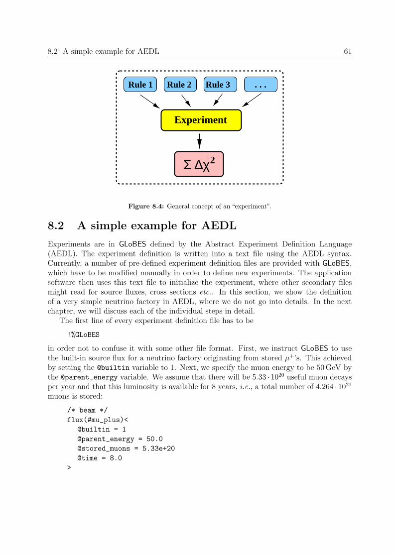
8.2 A simple example for AEDL 61
Rule 2Rule 1 Rule 3
Experiment
Σ ∆χ2
. . .
Figure 8.4: General concept of an “experiment”.
8.2 A simple example for AEDL
Experiments are in GLoBES defined by the Abstract Experiment Definition Language(AEDL). The experiment definition is written into a text file using the AEDL syntax.Currently, a number of pre-defined experiment definition files are provided with GLoBES,which have to be modified manually in order to define new experiments. The applicationsoftware then uses this text file to initialize the experiment, where other secondary filesmight read for source fluxes, cross sections etc.. In this section, we show the definitionof a very simple neutrino factory in AEDL, where we do not go into details. In the nextchapter, we will discuss each of the individual steps in detail.
The first line of every experiment definition file has to be
!%GLoBES
in order not to confuse it with some other file format. First, we instruct GLoBES to usethe built-in source flux for a neutrino factory originating from stored µ+’s. This achievedby setting the @builtin variable to 1. Next, we specify the muon energy to be 50 GeV bythe @parent_energy variable. We assume that there will be 5.33 · 1020 useful muon decaysper year and that this luminosity is available for 8 years, i.e., a total number of 4.264 · 1021
muons is stored:
/* beam */
flux(#mu_plus)<
@builtin = 1
@parent_energy = 50.0
@stored_muons = 5.33e+20
@time = 8.0
>

62 CHAPTER 8. Getting started
Note that we tell GLoBES that we want to refer to this neutrino source later as as #mu_plus.Let us now define a very simple detector with a target mass of 50 kt and 20 energy binsbetween 4 GeV and 50 GeV:
$target_mass = 50
$bins = 20
$emin = 4.0
$emax = 50.0
Then we specify the file which contains the cross sections we want to use:
/* cross section */
cross(#CC)<
@cross_file = "XCC.dat"
>
The command cross tells the parser that a cross section environment begins. It has thename #CC, which can later be used to refer to this specific environment, and thus to thefile XCC.dat. Note that each name begins with a leading #. Of course, the baseline andmatter profile have to be specified, too, where we use an arbitrary matter density profilehere:
/* baseline */
$profiletype = 3
$densitytab = {3.5}
$lengthtab = {3000.0}
The curly brackets used for the definition of $densitytab and $lengthtab refer to a list ofnumbers. Here, the lists contain only one element, because we only use one density layer:We initialize a baseline length of 3000 km with a constant matter density of 3.5 g/cm3. Asanother ingredient, we have to define the energy resolution function:
/* energy resolution */
energy(#MINOS)<
@type = 1
@sigma_e = {0.15,0.0,0.0}
>
The energy command starts the energy environment, which has the name #MINOS here.Out of several possibilities, it uses algorithm one, the simplest and fastest one. The actualenergy resolution is specified by the energy resolution variable, which is a list of threeelements. Each element is one parameter of the general resolution function as defined inEq. 9.12. Now we have all pieces to be able to define the appearance and the correspondingdisappearance channel of a neutrino factory: νe → νµ and νµ → νµ (µ+ stored).
8.2 A simple example for AEDL 63
/* channels */
channel(#appearance)<
@channel = #mu_plus: +: electron: muon: #CC: #MINOS
>
channel(#disappearance)<
@channel = #mu_plus: -: muon: muon: #CC: #MINOS
>
The first element is the name of the flux, which we have defined above. The secondelement “±” determines whether neutrinos or anti-neutrinos are taken from the flux table(two different polarities allowed). The third position defines the initial flavor, and the forthposition the final flavor, followed by the name of the cross section and energy resolutionfunction as defined before. The last step is to encapsulate the channels into a rule:
/* rules */
rule(#rule1)<
@signal = 0.45 @ #appearance
@signalerror = 0.001 : 0.0001
@background = 1.0e-05 @ #disappearance
@backgroundcenter = 1 : 0.0
@backgrounderror = 0.05 : 0.0001
@errordim_sys_on = 0
@errordim_sys_off = 2
@energy_window = 4.0 : 50.0
>
The @signal refers to the “signal” in our experiment. We use the above defined channelnamed #appearance with an constant overall efficiency of 0.45. The signal error variablehas two components: The first one is the normalization error of the signal, here 0.1%. Thesecond one refers to the energy calibration error of the signal, which is defined in Sec. 9.5.The background variable specifies the composition of the beam background. In this (sim-plified) case, we use the fraction 1 · 10−5 of the channel named #disappearance, i.e., themuon neutrinos with a mis-identified charge. The background center variable allows torescale the total background contribution from all background components simultaneously.It is only useful if there is more than one background component, otherwise it is usually 1.The background error variable is defined such as the signal error variable, i.e. we have a 5%background uncertainty and a very small energy calibration error. The “error dimensionvariable” @errordim_sys_X selects how the systematical errors are treated (cf., Table 9.2).
The here defined experiment represents a first simplified version of a neutrino factoryexperiment. It still lacks the correct energy dependence of the efficiencies, the antineutrinodisappearance channel, and the channels and rules for the symmetric operation with µ−
stored. However, it may serve as a simple, introductory example. In the next chapter, wewill demonstrate that the AEDL is much more powerful than illustrated here.

64 CHAPTER 8. Getting started
8.3 Introduction to the syntax of AEDL
We now give a short introduction to the syntax of AEDL. The first eight characters haveto be %!GLoBES in order to avoid parsing megabytes of chunk and producing thousands oferror messages. Comments can be used such as in C:
/* This starts a comment
and here the comment ends */
There are pre-defined variables which all start with $. Their range is also checked. Forexample, $bins can be only between 0 and 500.2 If one uses a float quantity where an int
is expected, the float will be converted to an int in the same way as in C. For example,we have scalar variables
$bins = 10
$baseline = 1200.0
and simple lists
$densitytab={1.0,2.2343,3.3432}
Since there are often groups of data which we want to refer to later, environments can beused. This is illustrated with the channel definition part:
channel(#ch1)<
. . .>
The first part is the type of environment, which is channel here. There are the followingtypes of environment in AEDL:
flux
cross
channel
energy
rule
Besides the environment type, there is a user-defined name beginning with # in the aboveexample: #ch1. It can be used later to refer to the channel defined in <. . .>. Those namesare so-called “automatic variables” and have to start with #. Note that these names haveto be unique and can only be refered to after their definition. However, similar to C, onecan give a declaration without definition before:
channel(#ch2)<>
2The upper limit is only there for safety reasons, the memory is allocated dynamically.

8.3 Introduction to the syntax of AEDL 65
Now one can refer to the name #ch2, while the actual channel definition comes later. Theinternal representation of this automatic variable is a number, which obtains its valuefrom a counter for each type of environment. For example, for channel the counter isnumofchannels. The counter keeps track of how many different names there are for onetype of environment, which means that it counts the number of channels, rules, energyresolution functions etc.. Thus, the automatic variables are numbered in the order of theirdefinition, and the number can later be used to refer to them in the C code (from 0 tonumof...−1). In order to facilitate the the mapping from names in AEDL to indices in Cthere are two functions glbNameToValue and glbValueToName which make this transition(see Sec. 6.2, page 43).
Within each environment type, there are several variables beginning with @, which canonly be used within the appropriate type of environment. In many cases, they have aspecial syntax, such as @channel.
If you want to have several experiments in one file, separate the different experimentsby
#NEXT#
This command resets the counters for channels, rules, fluxes, cross section and energy res-olution environments. All variables have their scope limited by either %!GLoBES, #NEXT#
or EOF. This allows a consistent treatment of various experiments in one file.As another feature of AEDL one can use include files with the include command.
Includes can be nested up to MAX_INCLUSION_DEPTH, which is currently set to 10. Errorreporting works for nested includes, too. The included file is not required to begin with%!GLoBES to facilitate cut and paste:
include "./file_1"
With this include mechanism, one can use constructions such as
include "NuFact.gls"
#NEXT#
include "JHFHK.gls"
in order to initialize a combined analysis of the experiments defined in the files NuFact.glsand JHFHK.gls. Note that one has to use quotation marks for filenames in AEDL. Evenif one uses the automatic variable #CC in both experiments, but the cross section data aredifferent (for example, because of different target nuclei), the correct cross section data willbe applied to each of the experiments. Note that, alternatively, one can also load both filessuccessively by two separate calls of glbInitExperiment.
Furthermore, one can define constants such as
Pi = 3.141
These constants can not only be defined within one AEDL file, but also by the calling Cprogram, which allows to use a simple but powerful variable substitution mechanism asdescribed in Sec. 7.3.
In addition, some simple algebraic manipulations are possible, such as

66 CHAPTER 8. Getting started
Pi+1
Pi^2
sin(Pi/2)
The following mathematical functions from <math.h> are available: sin, cos, tan, asin,acos, atan, log, log10, exp, sqrt.
These functions can be used everywhere, where otherwise only a scalar number wouldappear. However, they can not be applied to lists, such as sin({1,2,3}) will not work.
Finally, note that a line feed character \n is necessary at the end of the input – alter-natively you can put a comment at the end.

67
Chapter 9
Experiment definition with AEDL
In this chapter, we give a detailed definition of the AEDL features. We also show theunderlying mathematical concepts, where applicable. We do not exactly follow the separa-tion of source, oscillation, and detection properties, since most issues more or less involvethe detection. Instead, we illustrate many of the features of the GLoBES simulation suc-cessively in the logical order of their definition, and demonstrate how they translate intoAEDL .
9.1 Source properties and integrated luminosity
As we have disussed before, GLoBES can only deal with point sources. Thus, it is notpossible to study effects from the finite size of the neutrino production region, such as inthe sun or in reactor experiments with many neutrino sources (e.g., KamLAND). Therefore,a neutrino source in GLoBES can, in general, be characterized by the flux spectrum for eachneutrino flavor, the CP sign (neutrinos or antineutrinos), and the total luminosity of thesource.
Before we come to the definition of the source properties, let us discuss the total inte-grated luminosity of the experiment. In GLoBES, the total number of events is in generalproportional to the product of
Fid. detector mass [kt/t]× Running time [yr]×{
Source power [MW/GW]Useful muon decays [yr−1]
. (9.1)
Thus, the source power corresponds to either the amount of energy produced per timeframe in the target (such as for nuclear reactors or sources based on pion decay), or theuseful muon decays per time frame (neutrino factories). In addition, the definition of thesource power makes only sense together with the flux normalization, the running time,and fiducial detector mass in order to define the total integrated luminosity. Therefore,one can, in principle, use arbitrary units for these components as long as their productgives the wanted neutrino flux. However, it is recommended to use normalizations suchthat the source power units are MW for a proton-based beam, and GWthermal for a reactor

68 CHAPTER 9. Experiment definition with AEDL
experiment. Correspondingly, the detector mass units should be kilotons for a proton-basedbeam, and tons for a reactor experiment. In any case it is a good idea to document thechoices made by the user by corresponding comments in AEDL.
The quantity which can be used to scale the overall integrated luminosity of an exper-iment, is the fiducial detector mass. For example,
$target_mass = 50.0
defines a 50 kt detector for a neutrino factory.There are two principal ways to initialize a neutrino flux: Either one can use a built-in
source, or one can provide a file. In both cases, a flux is defined by the environment flux,such as
flux(#name)<
. . .@time = 8.0
>
with a running time of 8 years. Note that the running time is used within the flux envi-ronment. This feature can be used to load the neutrino and antineutrino fluxes separately,in order to combine them with different running times within one experiment. The nameof the flux #name will later be refered to in the channel definitions.
For a built-in neutrino source, one has to specify which built-in spectrum has to beused, as well as its parameters. The software will then automatically calculate the neutrinospectrum. Note that in this case, there is no degree of freedom in the choice of the sourceunits. Currently, two built-in fluxes are available: µ+-decay (@builtin = 1) and µ−-decay(@builtin = 2). In these cases, the muon energy (enery of the parent particle) has to bespecified together with the number of useful decays per year. Thus, an example to set upa neutrino factory flux is
flux(#mu_plus)<
@builtin = 1
@parent_energy = 50.0
@stored_muons = 5.33e+20
@time = 8.0
>
For a user-defined flux, one has to give it the file name:
flux(#user)<
@flux_file = "user_file_1.dat"
@time = 2.0
@power = 4.0
@norm = 1e+8
>

9.2 Baseline and matter density profile 69
In this case, the @norm variable is an overall normalization which defines a conversion factorfrom the fluxes in the file to the units in GLoBES. In general, there are many ways to givethe source power of a neutrino source, such as neutrinos per proton on target per area pertime frame. Right now, each flux has its own normalization factor, which is not alwaysstraightfoward to calculate. Often, one has to take into account many things, such as thenumber of target particles per unit mass. In addition, the fluxes will be rescaled by 1/L2,which means that the normalization must contain a factor L2
0. Here L0 is the distance fromthe source for which the flux is given to the actual neutrino production region. At the end,it is left to the user to ensure that the numbers in the flux file give, after the multiplicationwith @norm, the proper numbers of produced neutrinos corresponding to the chosen targetpower @power. Usually this adjustment of @norm is performed by comparison with knownenergy spectra for a specific experiment.
The software assumes that the given flux file has seven columns and 501 lines withequidistant energies. The format is:
E Φνe Φνµ Φντ Φνe Φνµ Φντ
In order to access fluxes at arbitrary energies, linear interpolation is used by the software.In general, it is advisable to provide the flux between $sampling_min and $sampling_max
(cf., Sec. 9.5), since these values are used by the software. However, if the energy leavesthe range of values given in the file, zero is returned. The the columns for the fluxes forunused flavours have to be filled all the same,e.g. with zeros.
The flux files accept one-line comments, which start with # and end with the linefeedcharacter ‘\n’, they are not counted as a line and their content is discarded. This commentsare useful to provide meta information about the fluxes like units or the origin of theinformation. This is also the default method to point the user to the references he/sheshould to cite when using a particular flux.
9.2 Baseline and matter density profile
The baseline and matter density profile determine, besides energy and involved flavors,the neutrino oscillation physics at the experiment description level. All of the neutrinooscillation parameters are defined at running time.
The baseline is given by
$baseline = 3000.0
Note that baseline lengths are always assumed to be in kilometers.Furthermore, the matter density profile along the baseline has to be specified. The
simplest matter density profile is a constant matter density profile with the average matterdensity from the PREM [2] onion shell model of the earth :
$profiletype=1

70 CHAPTER 9. Experiment definition with AEDL
$profiletype Additional variables Description1 $baseline Average density (constant)2 $baseline, $densitysteps PREM profile with given number of
equidistant steps3 $lengthtab, $densitytab Arbitrary profile (table of layer thick-
nesses, table of densities)
Table 9.1: Different matter density profiles which can be used with GLoBES.
If your using this option please cite reference [2].For a better approximation of the realistic earth matter density profile, one can use an
arbitrary number of equidistant steps of the PREM profile:
$profiletype=2
$densitysteps=20
Note that the value of $densitysteps is time-critical, since the computation time of oscil-lation probabilities is directly proportional to the number of layers. As a third possibility,one can specify the matter density profile manually with a list of thicknesses and densi-ties of the matter density layers. This example uses two density steps with two differentdensities:
$profiletype=3
$densitytab={2.8, 3.5}
$lengthtab={1000.0, 2000.0}
It is important that both lists have the same length and that the thicknesses given in$lengthtab add up to the length of the baseline, which does not have to be explicitelyspecified anymore. In addition, matter densities are always given in g/cm3. This approachcan also be used for a constant matter density profile with a specific matter density:
$profiletype=3
$densitytab={3.5}
$lengthtab={3000.0}
The possible options for matter density profiles are summarized in Table 9.1.
9.3 Cross sections
Cross sections will later be used as part of the channel definition (see Sec. 9.4). Similar tothe source fluxes, they are provided by the user as a data file:
cross(#name)<
@cross_file ="user_file_1.dat"
>

9.4 Oscillation channels 71
This cross section can later be refered to by #name.
Cross sections are in GLoBES given as differential cross section per energy:
σ(E) = σ(E)/E
[10−38 cm2
GeV2
](9.2)
The software assumes that the cross section files are text files with seven columns and 1001lines of the form
log10E σνe σνµ σντ σνe σνµ σντ
Here the logarithms of the energy values have to be equidistant. For arbitrary energies,linear interpolation is used. If the energy leaves the range of values given in the file, 0.0 willbe assumed. In general, it is advisable to provide the cross sections in the range between$sampling_min and $sampling_max (cf., Sec. 9.5). Unused cross sections have to be filledwith zeros, and can not be just omitted.
Like the flux files, the cross section files accept one-line comments, which start with #
and end with the linefeed character ‘\n’, they are not counted as a line and their content isdiscarded. This comments are useful to provide meta information about the cross sectionslike units or the origin of the information. This is also the default method to point theuser to the references he/she should to cite when using a particular cross section.
9.4 Oscillation channels
Channels in GLoBES represent an intermediate level between the pure oscillation physicsgiven by the oscillation probability Pαβ, and the total event rates composed of signal andbackground. A channel describes the path from one initial neutrino flavor in the sourceto the event rates in the detector for one specific interaction type (IT) and final flavor.Therefore, a channel contains the description of the initial neutrino flavor, its CP eigenvalue(neutrino or antineutrino)1, the detected neutrino flavor, the interaction cross sections forthe chosen interaction type, and the energy resolution function of the detector.
Before we come to the definition of the channel in AEDL, we introduce the generalconcept for the calculation of event rates. The first step is to compute the number ofevents for each IT in the detector for each initial and final neutrino flavor and energy bin.The second step is to include the detector effects coming from the insufficient knowledgein the event reconstruction. These two steps combined lead to the differential event ratespectrum for each initial and final flavor and IT as seen by the detector, which we call the“channel”. In this section, we focus on the first step, i.e., we discuss the definition of theenergy resolution function in the next section, since this is a rather comprehensive issue.
1Currently GLoBES does not support lepton number violating transitions, i.e. no transitions fromneutrino to antineutrino (or vice versa) are considered.

72 CHAPTER 9. Experiment definition with AEDL
The differential event rate for each channel is given by
dnITβ
dE ′ = N
∞∫0
∞∫0
dE dE Φα(E)︸ ︷︷ ︸Production
×
1
L2P(α→β)(E, L, ρ; θ23, θ12, θ13, ∆m2
31, ∆m221, δCP)︸ ︷︷ ︸
Propagation
×
σITf (E)kIT
f (E − E)︸ ︷︷ ︸Interaction
×
Tf (E)Vf (E − E ′)︸ ︷︷ ︸Detection
, (9.3)
where α is the initial flavor of the neutrino, β is the final flavor, Φα(E) is the flux of theinitial flavor at the source, L is the baseline length, N is a normalization factor, and ρ isthe matter density. The energies in this formula are given as follows:
• E is the incident neutrino energy, i.e., the actual energy of the incoming neutrino(which is not directly accessible to the experiment)
• E is the energy of the secondary particle
• E ′ is the reconstructed neutrino energy, i.e., the measured neutrino energy as ob-tained from the experiment
The interaction term is composed of two factors, which are the total cross section σITβ (E)
for the flavor f and the interaction type IT, and the energy distribution of the secondaryparticle kIT
β (E− E). The detector properties are modeled by the threshold function Tβ(E),coming from the the limited resolution or the cuts in the analysis, and the energy resolutionfunction Vβ(E − E ′) of the secondary particle.
Since it is a lot of effort to solve this double integral numerically, we split up the twointegrations. First, we evaluate the integral over E, where the only terms containing E arekIT
β (E − E), Tβ(E), and Vβ(E − E ′). We define:
RITβ (E, E ′) εIT
β (E ′) ≡∞∫
0
dE Tβ(E) kITβ (E − E) Vβ(E − E ′) . (9.4)
Thus, RITβ (E, E ′) describes the energy response of the detector, i.e., a neutrino with a (true)
energy E is reconstructed with an energy between E ′ and E ′ + dE ′ with a probabilityRIT
β (E, E ′)dE ′. The function R(E, E ′) is also often called “energy resolution function”.Actually, its internal representation in the software is a smearing matrix. The functionεITβ (E ′) will later be refered to as “post-smearing efficiencies”, since it will allow us to
define cuts and threshold functions after the smearing is performed, i.e., as function of E ′.
9.4 Oscillation channels 73
The detailed definition and initialization of the energy resolution function is described inSec. 9.5.
Eventually, we can write down the number of events per bin i and channel c as
nci =
∫ Ei+∆Ei/2
Ei−∆Ei/2
dE ′ dnITβ
dE ′ (E′) (9.5)
where ∆Ei is the bin size of the ith energy bin. This means that one has to solve theintegral
nci = N/L2
∫ Ei+∆Ei/2
Ei−∆Ei/2
dE ′
∞∫0
dE Φc(E) P c(E) σc(E) Rc(E, E ′) εc(E ′) . (9.6)
Note that the events are binned according to their reconstructed energy.A simple channel definition in GLoBES consists of the flux, the CP-sign of the ini-
tial state, the initial flavor, the final flavor, the cross sections, and the energy resolutionfunction. In order to refer to flux, cross sections, and energy resolution functions, theyhave to be defined before with their #name in the respective environments. Thus, a simpledefinition of a channel is
channel(#channel_1)<
@channel = #flux : +: muon: muon: #cross: #energy
>
It is also possible to define a channel as no-oscillation by using the prefix NOSC_ in eitherthe initial flavour or the final flavour, like this
channel(#channel_1)<
@channel = #flux : +: NOSC_muon: muon: #cross: #energy
>
In this case all diagonal probabilities Pαα are unity, and all off-diagonal probablities Pαβ
are zero. This is, for instance, useful for neutral current events, since these do not dependon any oscillation parameters2. The channels marked as NOSC_ are already computed byglbSetRates and do not have to be recomputed in the subsequent fit (which calls theundocumented function glbSetNewRates). Therefore this feature can be used to speedup the rate computation considerably, especially in cases where a large set of channelsexist which are only used for the computation of backgrounds. Usually it is an excellentapproximation to treat backgrounds as if they were not affected by oscillations3.
Note that the energy environment will be described in the next section. In addition,one can define pre- and post-smearing effects together with the channels, which will alsobe introduced together with the energy resolution function in the next section.
2At least in the absence of sterile neutrinos3In case, the backgrounds have a sizeable dependence on the oscillation parameters they carry infor-
mation on the oscillation parameters and are therefore more like a signal.
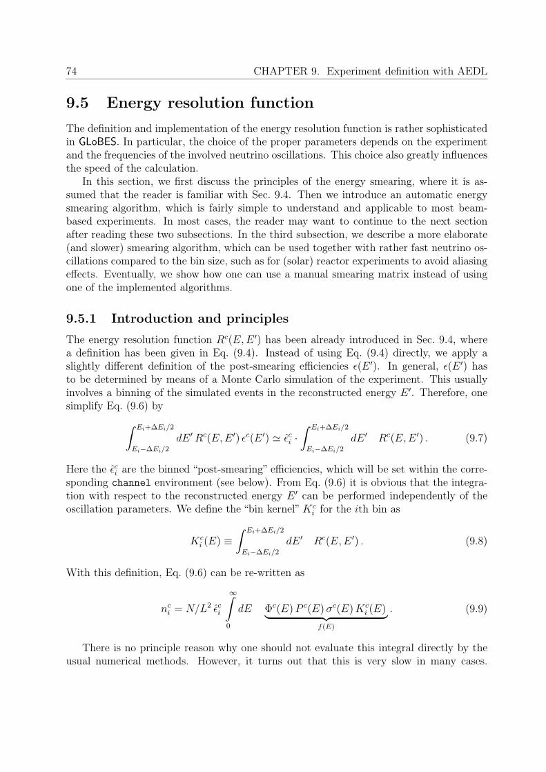
74 CHAPTER 9. Experiment definition with AEDL
9.5 Energy resolution function
The definition and implementation of the energy resolution function is rather sophisticatedin GLoBES. In particular, the choice of the proper parameters depends on the experimentand the frequencies of the involved neutrino oscillations. This choice also greatly influencesthe speed of the calculation.
In this section, we first discuss the principles of the energy smearing, where it is as-sumed that the reader is familiar with Sec. 9.4. Then we introduce an automatic energysmearing algorithm, which is fairly simple to understand and applicable to most beam-based experiments. In most cases, the reader may want to continue to the next sectionafter reading these two subsections. In the third subsection, we describe a more elaborate(and slower) smearing algorithm, which can be used together with rather fast neutrino os-cillations compared to the bin size, such as for (solar) reactor experiments to avoid aliasingeffects. Eventually, we show how one can use a manual smearing matrix instead of usingone of the implemented algorithms.
9.5.1 Introduction and principles
The energy resolution function Rc(E, E ′) has been already introduced in Sec. 9.4, wherea definition has been given in Eq. (9.4). Instead of using Eq. (9.4) directly, we apply aslightly different definition of the post-smearing efficiencies ε(E ′). In general, ε(E ′) hasto be determined by means of a Monte Carlo simulation of the experiment. This usuallyinvolves a binning of the simulated events in the reconstructed energy E ′. Therefore, onesimplify Eq. (9.6) by∫ Ei+∆Ei/2
Ei−∆Ei/2
dE ′ Rc(E, E ′) εc(E ′) ' εci ·∫ Ei+∆Ei/2
Ei−∆Ei/2
dE ′ Rc(E, E ′) . (9.7)
Here the εci are the binned “post-smearing” efficiencies, which will be set within the corre-
sponding channel environment (see below). From Eq. (9.6) it is obvious that the integra-tion with respect to the reconstructed energy E ′ can be performed independently of theoscillation parameters. We define the “bin kernel” Kc
i for the ith bin as
Kci (E) ≡
∫ Ei+∆Ei/2
Ei−∆Ei/2
dE ′ Rc(E, E ′) . (9.8)
With this definition, Eq. (9.6) can be re-written as
nci = N/L2 εc
i
∞∫0
dE Φc(E) P c(E) σc(E) Kci (E)︸ ︷︷ ︸
f(E)
. (9.9)
There is no principle reason why one should not evaluate this integral directly by theusual numerical methods. However, it turns out that this is very slow in many cases.
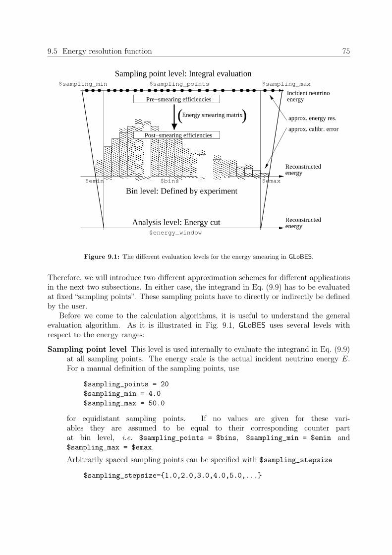
9.5 Energy resolution function 75
����������
����������
����
����
��������
��������
���������
���������
������������
������������
� �� �� �� �� �� �� �� �� �� �� �� �� �� �
� �� �� �� �� �� �� �� �� �� �� �� �
������������
����������
����������
�������
�������
������
������
�������
�������
� �� �� �� �� �
�����
� �� �� �� �� �� �
������
� �� �� �� �
� �� �� �� �
� �� �� �� �
� �� �� �� �
!!!
"""###
$$%%
&'(((((((((((
)))))))))))
**************
++++++++++++++
@energy_window
Analysis level: Energy cut
Post−smearing efficiencies
Pre−smearing efficiencies
Reconstructedenergy
energy
$bins$emin $emax
(Energy smearing matrix
Sampling point level: Integral evaluation$sampling_points$sampling_min $sampling_max
Incident neutrinoenergy
approx. energy res.
approx. calibr. error
Reconstructed
Bin level: Defined by experiment
)
Figure 9.1: The different evaluation levels for the energy smearing in GLoBES.
Therefore, we will introduce two different approximation schemes for different applicationsin the next two subsections. In either case, the integrand in Eq. (9.9) has to be evaluatedat fixed “sampling points”. These sampling points have to directly or indirectly be definedby the user.
Before we come to the calculation algorithms, it is useful to understand the generalevaluation algorithm. As it is illustrated in Fig. 9.1, GLoBES uses several levels withrespect to the energy ranges:
Sampling point level This level is used internally to evaluate the integrand in Eq. (9.9)at all sampling points. The energy scale is the actual incident neutrino energy E.For a manual definition of the sampling points, use
$sampling_points = 20
$sampling_min = 4.0
$sampling_max = 50.0
for equidistant sampling points. If no values are given for these vari-ables they are assumed to be equal to their corresponding counter partat bin level, i.e. $sampling_points = $bins, $sampling_min = $emin and$sampling_max = $emax.
Arbitrarily spaced sampling points can be specified with $sampling_stepsize
$sampling_stepsize={1.0,2.0,3.0,4.0,5.0,...}

76 CHAPTER 9. Experiment definition with AEDL
The choice of the sampling point configuration strongly depends on the experimentand required accuracy. Ideally the integrand of Eq. 9.9 is zero outside the samplingrange, if this cannot be achieved it is usually sufficient that the sampling range is byabout three times the energy resolution4 larger than the bin range. The spacing ofthe sampling points should be somewhat smaller (a factor ' 2 usually is more thanebough) than the finest details of the integrand.
Bin level This level is determined by the experiment and its analysis. Note that energybin sizes much smaller than the energy resolution will not improve the results. Theenergy bin range and the number of energy bins do always have to be specified. Forthe case of large values of the integrand in Eq. (9.9) at the energy range limits, it isrecommended to exceed the analysis energy window by about three times the energycalibration error in order to avoid cutoff effects.
In order to define a range between Emin and Emax divided by a certain number ofequidistant bins, use
$emin = 4.0
$emax = 50.0
$bins = 20
For arbitrary bins, use Emin and Emax and the size of each bin ∆Ei:
$emin = 4.0
$emax = 50.0
$binsize = { 15.0 , 5.0 , 20.0, 6.0 }
The number of bins will be automatically computed by GLoBES. Note that the binsizes have to add up to the energy range $emax-$emin.
The choices at bin level are mainly determined by optimizing the performance of theexperiment.
Analysis level On the analysis level, an energy window can be defined within each rule.For details, see next chapter.
In general, the energy smearing happens between the sampling point and bin levels,which means that the energy smearing matrix will have $sampling_points columns and$bins rows.
As illustrated in the figure, an interesting feature in combination with the chan-nels are pre- and post-smearing effects. Pre-smearing effects are taken into ac-count on the sampling point level, and post-smearing effects on the bin level. Ex-amples for these effects are energy dependent efficiencies and (non-beam) back-grounds. Efficiencies are multiplicative factors, whereas backgrounds are added to
4evaluated at $emin and $emax respectively
9.5 Energy resolution function 77
the event rates. These components can be introduced before or after the inte-gration in Eq. (9.9) is done. If they are introduced before, we call them@pre_smearing_efficiencies or @pre_smearing_background. If they are introduced af-ter, we call them @post_smearing_efficiencies or @post_smearing_background. Notethat pre-smearing components are always a function of the incident neutrino energy E.Thus, there have to be as many elements as there are sampling points. Examples for pre-smearing quantities are non-beam backgrounds, such as from geophysical neutrinos. Thepost-smearing components are always a function of the reconstructed neutrino energy E ′,such as the post-smearing efficiencies εIT
β (E ′) in Eq. (9.4). Examples for post-smearingefficiencies are cuts and detection threshold functions. All post-smearing components haveto have as many elements as there are energy bins. Efficiencies are multiplicative and theirdefault value is 1, whereas backgrounds are additive and their default value is 0. Thus, amore elaborate channel can be defined as
channel(#channel_1)<
@channel = #flux : +: muon: muon: #cross: #energy
@pre_smearing_background = {1,2,3,4,5,6,7,8,9,10}
@post_smearing_efficiencies = {0.1,0.2,0.3,0.4,0.5}
>
This experiment uses 10 sampling points and 5 bins.In the following subsections we will define the energy resolution function. All energy
resolution functions are defined within an energy environment and can be refered to by#name.
energy(#name)<
. . .>
The individual parameters of the environment will be defined below and depend on thealgorithm used.
9.5.2 Bin-based automatic energy smearing
This algorithm is the simplest of the built-in algorithms for the evaluation of Eq. (9.9). Itis applicable to most of the experiments which can be simulated with GLoBES.
The key idea is to use a “flat” model, i.e. the integrand of Eq. 9.9 is well approximatedby being piecewise constant in each sampling step. This is a good approximation as longas
• No details are lost, i.e. the spacing of sampling points is smaller than the energyresolution.
• The edges are treated correctly.
• The neutrino oscillations are slow on a scale of the smapling point distance.

78 CHAPTER 9. Experiment definition with AEDL
In this case, Eq. (9.9) is reduced to
nci = N/L2
N∑j=1
Φc(Ej) P c(Ej) σc(Ej) Kci (Ej) ∆Ej . (9.10)
The advantages of this algorithm are obvious: All factors independent of the oscillationparameters have to be only evaluated once at values of E which are known in advance,which means that they can be put into a look-up table. In addition, the probability hasto be only evaluated at previously known values of the energy, which makes it possible tocompute the transition amplitudes for all channels simultaneously. One assumption is thatall involved factors are piece-wise constant, i.e., they hardly change within each bin. Thisassumption seems to be very restrictive, which is however not quite correct. First of all, ifone analyzes simulated data (which are simulated with the same algorithm), the errors willcancel between the simulated and fitted data. Second, and more important, this algorithmis just a very basic integration routine5 and converges to the true result for decreasing stepsize. Thus if the number of sampling points is large enough this algorithm is very accurate.This algorithm is selected by
@type = 1
within the #energy environment. The computation of the bin kernel Kci is performed
by GLoBES. Thus, it requires that the number of bins $bins and the minimum energy$emin and maximum energy $emax are given in case of equidistant bins. As far as theparameterization for the energy resolution function Rc(E, E ′) in Eq. (9.8) is concerned, thealgorithm uses a Gaußian
Rc(E, E ′) =1
σ(E)√
2πe− (E−E′)2
2σ2(E) . (9.11)
There are several energy resolution functions available, where by default #standard isused:
@sigma_function = #standard
The energy resolution function #standard is defined by
σ(E) = α · E + β ·√
E + γ , (9.12)
where the parameters α, β and γ are provided by the user:
@sigma_e = {0.15, 0.0, 0.0}
5It is planed for to have something like a Gauß-Kronrod scheme as an alternative here.

9.5 Energy resolution function 79
Currently, another possible choice for @sigma_function is #inverse_beta, which onlyuses the parameter α. It is defined by
σ(E) =
{α ·√
1000−1√
x− 8 · 10−4 , for x > 1.8 · 10−3
α · 10−3 , for x ≤ 1.8 · 10−3(9.13)
The somewhat complicated form is due to the fact that inverse β-decay has a neutrinothreshold of 1.8 MeV and that a neutrino at threshold already produces ' 1 MeV visibleenergy in the detector (for more details see e.g. [6]).
In the actual implementation of the algorithm, the sum in Eq. (9.10) is only computedfor the Ej’s where K(Ej) is above a certain threshold, which is by default 10−7. Thisthreshold is defined at the compiling time.
Eventually, a complete energy resolution definition of this algorithm is, for example,
energy(#name)<
@type = 1
@sigma_function = #standard
@sigma_e = {0.15 ,0.0 ,0.0}
>
9.5.3 Low-pass filter
In order to ensure that fast oscillating probabilities do not lead to aliasing, it is possibleto impose a low-pass filter already during the calculation of the probabilities itself. Thisfilter is implemented has a highly experimental feature called “filter”. The calculation ofoscillation probabilities is, in principle, a computation of phase differences. Restricting themaximum admissible size of those phase differences effectively filters the high frequencycomponent of the oscillation probability. This idea is implemented according to
Pαβ(E) =∑ij
UαjU∗βjU
∗αiUβie
−iΦij × e−Φ2ij/σf (E)2 , (9.14)
where Φij := ∆m2ijL/2E is the usual phase difference and the last term is a Gaußian filter
with width σf (E). Choosing σf (E) := σ0f ·E ensures that this filter behaves approximately
such as an energy resolution function with constant width σe =√
2/σ0f , i.e.∫
dE P (E)1
σe
√2π
e− (E−E)2
2σ2e . (9.15)
The relationship between Eqs. 9.14 and 9.15 is not obvious and connected to the propertiesof Pαβ: see Refs. [10, 11]. This feature works only for vacuum and constant densities andis controlled by the filer state variable. In addition, σe is set by the filter value variable:
$filter_state = 1
$filter_value = 2.0

80 CHAPTER 9. Experiment definition with AEDL
would switch the filter feature on and set the width to 2.0 GeV. The setting of$filter_state is ignored whenever a density profile with more than one layer is used.
With a type 1 (@type = 1) energy resolution function, σe adds on to the energy reso-lution function of the detector σc(E) such as
σeff(E)2 ' σ2e + σc(E)2 . (9.16)
Sometimes this behavior is unwanted, and therefore one can try to ’subtract’ the filteringfrom the energy resolution function by splitting the energy resolution function σ(E)eff intwo parts by
σeff(E)2 = σc(E)2 − σ2e︸ ︷︷ ︸
σ2c (E)
+σ2e , (9.17)
where the truncated energy resolution function σc(E) is used instead of σc(E) in computingthe smearing data. Thus one obtains as effective energy resolution
σeff(E)2 ' σc(E)2 . (9.18)
This scheme is used by choosing as type for the energy resolution
@type = 2
9.5.4 Manual energy smearing
In some cases, one may use the output of a detector Monte Carlo simulation directly.Then one can use ”manual” energy smearing instead of the automatic energy smearingalgorithms.
The energy smearing matrix Kij has $bins rows and $sampling_points columns,which are numbered from 0 to $bins−1 or $sampling_points−1. It is equivalent to thebin- and sampling-point-based kernel in Eq. (9.8):
Kij = Kci (E)|E=Ej
, (9.19)
where Ej is the energy of the jth sampling point. In general, many of the entries in thismatrix are zero, which means that it is convenient to evaluate the integrand in Eq. (9.9)only at positions where Kij is non-zero. The corresponding “sampling range” range of non-zero matrix entries in Kij for the ith energy bin is defined to run from column ki
l (“lowerindex”) to column ki
u (“upper index”). An example for a smearing matrix is
Kij =
a00 a01 a02 a03
a10 a11 a12 a13 a14
a21 a22 a23 a24 a25
a32 a33 a34 a35 a36
a43 a44 a45 a46 a47
↑ . . . ↑ki
l kiu
︸ ︷︷ ︸
$sampling points columns
← $bins rows , (9.20)
9.6 Rules and the treatment of systematics 81
where the unshown entries are zero. Thus, the values of Kij have to be specified betweenki
l and kiu in the form {ki
l , kiu, Ki ki
l, Kiki
l+1, . . . , Kikiu}:
energy(#name)<
@energy = {0,2, 0.8634265, 0.0682827, 4e-06}:
{0,4, 0.1507103, 0.6965592, 0.1507103, 0.00101, 1e-07}:
. . .{40,42, 0.1507103, 0.6965592, 0.1507103};
>
The last line has to be terminated by a semicolon ‘;’. Note that the sum of all entriesin each column should be equal to unity, since all of the incoming neutrinos should beassigned to energy bins. In many practical cases, however, the definition of the energysmearing can lead to sums smaller than unity, such as in the case of truncated Gaußiandistributions. The sum of entries in each row is not defined, since the events might beunevently distributed into the energy bins according to the energy resolution function.
9.6 Rules and the treatment of systematics
The set of rules for an experiment is the final link between the event rate computation andthe statistical analysis. The information in the rules specifies how the χ2 is computed basedupon the raw event rates given by the channels and possible systematical errors. Therefore arule has two parts: The first part describes how signal and background events are composedout of the channels, and the second part specifies which systematical errors are considered,as well as their values. For a rule, the splitting in signal and background is useful for thetreatment of systematics, as we will se later. Each rule will lead to a ∆χ2-value, whichmeans that all ∆χ2’s of the different rules will be added for the whole experiment. Withineach rule, the event rates are added, and the systematics is considered to be independent ofthe other rules. Thus, it is convenient to combine the above defined channels for differentoscillation patterns and interaction types into one logical construction, which is the rule.For example, a superbeam usually has two rules: One for the νe-appearance rates, and onefor the νµ-disappearance rates. In each case, contributions of several interaction types, aswell as from the νe-contamination of the beam will lead to a number of contributing signaland background event channels.
For each rule, the signal event rate si in the ith bin can be composed out of one ormore channels by
si = αcs1 · ncs1i + αcs2 · ncs2
i + . . . (9.21)
where the α’s are overall normalization factors/efficiencies determined by the propertiesof the detector. Note that bin-based (energy-dependent) efficiencies can be defined withthe post-smearing efficiencies in the last section. In addition, note that in most cases, itmakes sense to have only one signal channel and to assign all sorts of perturbations to thebackground. Similarly, the background event rate bi in the ith bin can be composed out of

82 CHAPTER 9. Experiment definition with AEDL
one or more channels
bi = βcb1· ncb1
i + βcb2· ncb2
i + . . . , (9.22)
where the channels can be any combination of the ones in the signal rate and additionalones. The background normalization factors very often have a specific meaning. Forexample, they may correspond to a fraction of mis-identified events (charge or flavor mis-identification). These basic building blocks of each rule are, within the rule environment,for example defined by
@signal = 0.5 @ #channel_1
@background = 0.001 @ #channel_2 : 0.005 @ #channel_3
For the analysis of the systematical errors, the so called “pull method” is used [12]6. Forthe pull method, k systematical errors are included by introducing k additional variablesζk, which are the so-called “nuisance parameters”. The nuisance parameters describe thedependence of the event rates on the various sources of systematical errors, such as anerror on the total normalization is included by multiplying the expected number of eventsin each bin by a factor (1 + ζ1). The variation of ζ1 is in the fit constrained by addinga penalty p1 to the χ2-function. In case of a Gaußian distributed systematical error, thispenalty is given by
pi =(ζi − ζ0
i )2
σ2ζi
, (9.23)
where ζ0i denotes the mean and σζi
the standard deviation of the corresponding nuisanceparameter. We further on also refer to the mean as the “central value”, and to the standarddeviation as the“error”. The latter corresponds to the actual systematical uncertainty. Theresulting χ2 is then minimized with respect to all nuisance parameters ζi, which leads toχ2
pull
χ2pull(λ) := min
{ζi}
(χ2(λ, ζ1, . . . , ζk) +
k∑j=1
pj(ζj)
). (9.24)
Here λ refers to the oscillation parameters including the matter density ρ. One advantageof the pull method is that whenever the number N of data points is much larger than k,it is numerically easier to compute χ2
pull than to invert the N ×N covariance matrix. Forthe experiments considered here, N is typically 20 and k ∼ 4, which means that the pullmethod is numerically much faster. Moreover, it is more flexible and allows the inclusion ofsystematical errors also for a Poissonian χ2-function. In Ref. [12], it has been demonstratedthat the pull method and the covariance based approach are equivalent for a Gaußian andlinear model. In general, there is a separate (χ2
pull)r for each rule r, i.e., pair of signal
and background spectra, with a separate set of nuisance parameters ζαi . Thus, χ2
pull is thesum of all individual (χ2
pull)r’s. By the minimization, the dependence on the k nuisance
parameters has been eliminated from χ2pull.
6In fact the pull method was employed already in Ref. [5] before Ref. [12] appeared.
9.6 Rules and the treatment of systematics 83
Now we can introduce the different systematical errors. The two most important andmost easily parameterized systematical errors are the normalization and an energy calibra-tion errors. These errors are assumed to be independent between the signal events and thebackground events, which means that this systematics treatment defines the grouping intosignal or background. The implementation of the normalization error is straightforward:
si(a) := a · si (9.25)
with an analogous definition for the background events. Here, a is the“nuisance”parameter,which will be minimized over later.
For the parameterization of an energy calibration error, two possibilities are imple-mented. The first one (method “T”) is somewhat simpler, whereas the second one (method“C”) is more accurate, but it requires a careful choice of parameters. The first option(method “T”) is
si(a, b) ≡ si(a) + b · si E′i/(E
′max − E ′
min), (9.26)
where E ′min and E ′
max correspond to $emin and $emax, and E ′i is the mean (reconstructed)
energy of the ith bin. It is often refered to as a “tilt” of the spectrum, since it describes alinear distortion of the event rate spectrum. Note that this definition of a tilt makes onlysense in combination with a large enough normalization error, since the tilt also affects thenormalization. The second option (method “C”) is closer to an actual energy calibrationerror, which means that one should test this option whenever one suspects a large impactof this systematical error. It is based upon replacing the events in the ith bin by the onesat the energy (1 + b) ·E ′
i. If this target energy does not exactly hit a (discrete) bin energyEk, linear interpolation is used. We use the following approximation:
si(a, b) = (1 + b) · [(sk+1(a)− sk(a)) · (δ − k) + sk(a)] , (9.27)
δ = b · (i + t0 + 1/2) + i ,
k = div(δ, 1) ,
t0 = E ′min/∆E0 .
Here ∆E0 is the bin width ($emax-$emin)/$bins and “div” refers to the integer part of thedivision. Note that the factor (1 + b) in the first equation comes from a renormalizationof the bin width, since also the bin width is altered by the replacement of the energies.Furthermore, special care has to be payed to the limits k < 1 or k + 1 > Nbins, since theresk or sk+1 may not have been calculated. By default, it is assumed that sk is zero in thosecases. However, if the event rates are still large at the limits, errors will be introducedleading to a wrong estimate of the impact of the calibration error. In this case, one shouldtruncate the analysis range by a few bins at the boundaries and therefore ensure in thisway that only those si are used whose index k is within the range 0, . . . , Nbins − 1 (cf.,Fig. 9.1). Thus, it is possible to constrain the analysis energy range with each rule to anenergy window:
@energy_window = 4.0 : 50.0

84 CHAPTER 9. Experiment definition with AEDL
The default energy window is given between the minimal and maximal reconstructed en-ergy. To be on the save side, reduce analysis window compared to the bin range on eachside by about three times the energy calibration error.
Eventually, the total event rate xi in a bin i is given by
xi(a, b, c, d) = si(a, b) + bi(c, d) , (9.28)
and is thus a function of four parameters. The four parameters a, b, c, d have been intro-duced in order to describe systematical uncertainties and are the nuisance parameters. Eachof the four parameters has a central value and systematical error. The central values for allof the four parameters have to be always defined. They are called signal normalization (a),signal tilt/calibration (b), background normalization (c) and background tilt/calibration(d). The default values are
a = 1 , b = 0 , c = not assigned , d = 0 . (9.29)
Thus, for the background normalization c, the value has to be specified in either case.The values for the normalization and the values of tilt/calibration are always regarded asa pairs, i.e., they are given in the form normalization : tilt. The errors are treatedin the same way. For example, we have
@signalerror = 0.001 : 0.01
@backgroundcenter = 0.1 : 0.0
@backgrounderror = 0.001 : 0.01
There is no @signalcenter in this definition, since by default the central value for thesignal normalization is 1 and the central value for the tilt/calibration is 0.
The user has the possibility to choose the set {ζi} of nuisance parameters which areminimized over. This choice is specified with the error dimension variable, and the differentpossibilities are shown in Table 9.2. Since the error dimension defines the treatement ofsystematics it is useful to have define a matched pair of error dimensions for each rule, whereon value describes how the event rate is computed for no systematics and the other one iswith systematics (see also Sec. 7.2). The error dimensions for the case of no systematicsis set for each rule by the value of @errordim_sys_off, whereas the error dimension forsystematics on is given by @errordim_sys_on . Thus, for example, the complete errordimension definition could look like
@errordim_sys_off = 2
@errordim_sys_on = 0
It is foreseen to add the possiblity to extend the set of error dimensions or the set of possiblesystematical errors in one of the next versions of GLoBES.
Eventually, a rule looks like

9.7 Version control in AEDL files 85
Error dimension a b c d Tilt/Calibration Remarks
0 + + + + T Systematics with tilt2 - - - - - No systematics4 + + + + T Total rates7 ∞ - ∞ - - Spectrum only8 - - - - - Total rates, No systematics9 + + + + C Systematics with calibration
Table 9.2: Possible values of the error dimensions variable in GLoBES and their meaning. If a parameteris designated with +, it will be marginalized over, and therefore the corresponding error needs to have anon-zero value. If the cases with “total rates” in the remarks, the summation over the bins is performedbefore computing the χ2, i.e., no spectral information is used. The error dimension 7 “spectrum only”leaves the normalization free (σa = σc = ∞), and therefore only the spectral information is used. As aconsequence, the settings for the normalization error will be ignored (designated with the symbol ∞).
rule(#rule_1)<
@signal = 0.5 @ #channel_1
@background = 0.001 @ #channel_2 : 0.005 @ #channel_3
@signalerror = 0.001 : 0.01
@backgroundcenter = 0.1 : 0.0
@backgrounderror = 0.001 : 0.01
@errordim_sys_off = 2
@errordim_sys_on = 0
@energy_window = 4.0 : 50.0
>
9.7 Version control in AEDL files
In order to avoid problems which come from different versions of GLoBES and AEDL files,it is possible to use in each AEDL file a version number. For example, it may correspondto the minimum version number of the GLoBES package with which it works. Set the$version by
$version="1.8.1"
This information can be accessed by the versioning functions as described in Sec. 2.5.

86 CHAPTER 9. Experiment definition with AEDL
87
Chapter 10
Testing & debugging of AEDL files
AEDL is a powerful language to describe a variety of different experiments. This chapterdemonstrates how to test an AEDL file in order to check if it really describes a givenexperiment. For this application, the GLoBES package contains the program globes. Itcan either be regarded as an AEDL debugger, or as a simple command-line oriented tool toconvert the rather abstract AEDL experiment description into more accessible event rates.
10.1 Basic usage of the globes binary
The globes binary is installed together with the library, but into the directory$prefix/bin/. In order to use the globes utility, this directory has to be in the pathof the shell used to call the program.1
As an argument, globes takes a .glb-file. While parsing it, it prints any warnings anderrors which have occured during reading the file. Then it uses the experiment descriptionin the file to compute the event rates at a certain point in parameter space. Finally, itdisplays the result based on the options used to call globes. The options of globes followthe GNU standard. Thus, there is a --help option to display all other options togetherwith short descriptions.
Calling globes without any options and with a .glb-file as argument produces an eventsummary at rule level. In this case, the full experiment description in the file is taken intoaccount, i.e., all efficiencies, backgrounds, and energy resolution effects. Thus, the returnedevent rates are the ones which will be actually used to compute the χ2 later. By default,the oscillation parameters used to calculate the transition probability are
sin2 2θ12 = 0.8 ∆m221 = 7 · 10−5 eV2 ,
sin2 2θ23 = 1.0 ∆m231 = 3 · 10−3 eV2 ,
δ = 0 sin2 2θ13 = 0.1 . (10.1)
1This is automatically the case if no options are given to configure, and make install was executedwith root-privilege, i.e., a standard installation was done.

88 CHAPTER 10. Testing & debugging of AEDL files
Of course, it is possible to change these default values either by using the option -p on acall by call basis, or by setting the environment variable GLB_CENTRAL_VALUES:
globes -p’0.55,0,0.785,0,0.0008,0.0025’
globes --parameters=’0.55,0,0.785,0,0.0008,0.0025’
For example, GLB_CENTRAL_VALUES can be defined within the shell session or in the shellprofile:
export GLB_CENTRAL_VALUES=’0.55,0,0.785,0,0.0008,0.0025’
Furthermore it is possible to switch off oscillations with the -N option and to switch themon again with -O (the default). The effect of -N is the same as to use NOSC_ in all oscillationchannels. Thi feature is useful if one wants to normalize an expriment flux if the numberof un-oscillated events is given.
The AEDL parser and interpreter have basically three levels of messages to the user:Warnings, errors and fatal errors. Fatal errors are always reported and lead to a programexit with status ’1’. Usually only errors and no warnings are reported. The verbosity levelcan be chosen by the -v option, where -v1 is default, i.e., only errors and fatal errorsare reported. The level -v0 corresponds to reporting fatal errors only, and -v2 will printwarnings in addition to fatal errors. It is recommended to test any new .glb-file with -v2
to check the warnings at least once, and to decide whether there is a problem to be fixed.With -v3 all files read by globes are displayed together with their path, and with -v4
all files which have been attempted to be read are shown. These two setting are useful toclarify path resolution issues and shadowing of file names.
10.2 Testing AEDL files
In the process of defining a new experiment, the default output of globes at rule level isthe final step. However, in order to arrive at this level it is often necessary to review theintermediate steps in the event rate calculation. The globes utility offers many possibilitiesto do this based on the rate access functions as described in Sec. 6.3.
By default, globes returns total rates corresponding to the -t option. This can bechanged to to a full spectrum by using -s. The spectral rates are shown in a table wherethe first column always gives the central energy of the corresponding bin or the samplingpoint.
If there is more than one experiment in a file, i.e., there is at least one #NEXT# command,only the event rates for one experiment will be shown. This experiment can be chosen withthe -e option, which takes as a mandatory argument the number of the experiment (startingwith zero). The default is -e0.
Channel level
As a first step, one may want to check if each channel produces the anticipated output.Channel rates are returned if the -c option is used. This option takes as an optional

10.2 Testing AEDL files 89
argument the channel number (starting at zero). If no argument is given all channels aredisplayed. By default, the sum of the event rates in each channel is shown. Each columnhas as first line the same channel name as in the file.
It is also possible to switch off one detector effect after the other. First, one can switchoff the post-smearing efficiencies (-f) and the post-smearing backgrounds (-g). Next,one can switch off the energy resolution function with (-b) and view the rates beforesmearing. If the -s option is also used, the number of lines in the output will be given by$sampling_points. Another effect of the -b option is that the post-smearing efficienciesand backgrounds are no longer taken into account. Therefore, the -g and -f options nowapply to the pre-smearing efficiencies and the pre-smearing backgrounds. Thus,
globes -c -b -g -f FILE
produces the raw event rate corresponding to the convolution of flux, probability, and crosssection, which is neglecting all detector effects.
Rule level
The next logical step after checking the channel rates is to investigate the rule rates. Therule rates are returned with the option -r. This option takes as an optional argument therule number (starting at zero). If no argument is given, all rules will be displayed. Bydefault, the sum of the event rates in each rule is shown, as well as for each componentwithin the rule. Each rule is preceeded by a line with the same rule name as in the file.
It is also possible for rules to switch off one detector effect after the other – with thelimitation that rules only make sense after the energy resolution function has been appliedto each channel. Therefore, it is not possible to use -b together with -r, or to switchoff any pre-smearing efficiencies or backgrounds. One can, however, switch off the post-smearing efficiencies (-f) and the post-smearing backgrounds (-g) for each channel. Sincethe definition of a rule also contains so-called “coefficients”, it is possible to switch themoff with -i. This options also deactivates any setting of @backgroundcenter.
Output
The default output stream is stdout. The output can be re-directed to a file using the -o
option, which takes as mandatory argument the file name. The default output format aimsat maximal readability for a human eye. In many cases however, the output of globes isproduced as input for other programs. There are some features to adjust the output format.Usually one would like to omit the channel and rule names by using simple printing -S
instead of pretty printing -P.There are special options for certain special formats: -m produces Mathematica2 list
output, which can be directly visualized by MultipleListPlot. The option -u uses thesame principal formatting as -m, but it allows to specify the left, middle, and right delimitersin constructing the list, such as
2Mathematica is a trademark of Wolfram Inc.

90 CHAPTER 10. Testing & debugging of AEDL files
left
left 1 middle 2 middle 3 right
middle
left
left 1 middle 2 middle 3 right
right
This is, with left = ’{’, middle = ’,’ and right = ’}’, equivalent to the list{{1, 2, 3}, {1, 2, 3}}. The delimiters can be set by -L, -M and -R as in the following example:
globes -Su -R$’\n’ --Middle=" " -L" " ...
Here $’\n’ is the escape sequence in the shell for ANSI C-like characters, such as linefeed’\n’. The above example produces a a two column file such as
1.0 0.121.2 0.141.3 0.18...
where the first column is the central energy of the bin or the sampling point, and thesecond column gives the event rate. Usually, the output is a concatenation of many suchtwo columns tables, where each rule part or channel part has its own table. Thus one can,by using -u and user-defined delimiters, construct many different output formats.
AEDL external variable substitution
Some .glb-files use external AEDL variables in order to allow special purpose studies (suchas the energy resolution-dependence). If the external variables are not explicitely specified,they are interpreted by the parser as zeros. Thus, it is impossible to properly parse anyfiles with globes which contain such undefined variables. Hence, there is the possibility todefine AEDL variables by using the define option -D. A call such as
globes -DBASELINE=3000 ...
would define the AEDL variable BASELINE to be 3000.

91
Acknowledgments
We would like to thank Martin Freund, who wrote the very first version of a three-flavourmatter profile treatment many years ago. PH is especially thankful for the invaluableadvice of Thomas Fischbacher on many design issues. In addition, we would like to thankMark Rolinec for his help to translate the experiment descriptions into AEDL, and forcreating the illustrations in this manuscript. Finally, thanks to all the people who havebeen pushing this project for many years, to the ones who have been continuing asking forthe publication of the software, and the referees of several of our papers for suggestionswhich lead to improvements in the software.
This work and the development of GLoBES have been supported by:
• Physik Department der Technischen Universitat Munchen
• Max-Planck-Institut fur Physik
• Sonderforschungsbereich 375 fur Astro-Teilchenphysikder Deutschen Forschungsgemeinschaft
• Studienstiftung des Deutschen Volkes
• Institute for Advanced Study, Princeton
• W. M. Keck Foundation
• Physics Department of the University of Wisconsin, Madison

92 CHAPTER 10. Testing & debugging of AEDL files

93
GLoBES installation
The installation of GLoBES is highly automated and there should not be any problems ona decently up-to-date GNU/Linux system. The installation has, however, only been testedon a limited number of platforms. The current version has been tested for SuSE, Red Hat,Fedora Core and a 64bit version of SuSE. It should also compile and work on Mac OS.We would appreciate to know your experiences with the installation on different platforms.Please send an e-mail to <[email protected]>.
Prerequisites for the installation of GLoBES
Besides the usual things such as a working libc, you need to have
gcc The GNU compiler collectiongcc.gnu.org
GSL The GNU Scientific Librarywww.gnu.org/software/gsl/
The library libglobes should in principle compile with any ANSI C/C++ compiler, butthe globes binary uses the argp facility of glibc to parse its command line options.However, on platforms where argp is lacking GLoBES has replacement code, thus it shouldalso work there.
All those libraries are also available as rpm’s from the various distributors ofGNU/Linux, see their web sites for downloads. Chances are that gcc and GSL are alreadypart of your installation. For building GLoBES from source, however, not only workinglibaries for above packages are needed but also the headers, especially for GSL. Dependingon your installation, eg. on RedHat/Fedora, of GSL this may require to additionally installa rpm-package named gsl-devel. If GSL has been installed from the tar-ball as providedby gnu.org no problems should occur. Furthmore you need a working make to build andinstall GLoBES.
Installation Instructions
GLoBES follows the standard GNU installation procedure. To compile GLoBES you willneed gcc. After unpacking the distribution the Makefiles can be prepared using the con-

94 CHAPTER . GLoBES installation
figure command,
./configure
You can then build the library by typing,
make
A shared version of the library will be compiled by default.The library can be installed using the command,
make install
The default install directory prefix is /usr/local. Consult the ”Further Information”section below for instructions on installing the library in another location or changingother default compilation options.
The install target also will install a program with name globes to $prefix/bin andthe files in the data directory of the tar-ball to $prefix/share/globes.
If you are not using make install you will find the static libary atsource/.lib/libglobes.a which you can copy to any destination. However keep inmind that the linking command will be somewhat different, i.e. you have to specify allthe dynamically linked objects besides libglobes.
The default install directory prefix is /usr/local. Consult the ”Further Information”section below for instructions on installing the library in another location or changing otherdefault compilation options.
Moreover a config-script called globes-config will be installed. This script displaysall information necessary to link any program with GLoBES. For building static libariesand linking against them see the corresponding section of this file.
Basic Installation
The configure shell script attempts to guess correct values for various system-dependentvariables used during compilation. It uses these values to create a Makefile in eachdirectory of the package. Finally, it creates a shell script config.status that you canrun in the future to recreate the current configuration, a file config.cache that saves theresults of its tests to speed up reconfiguring, and a file config.log containing compileroutput (useful mainly for debugging configure).
If you need to do unusual things to compile the package, please try to figure outhow configure could check whether to do them, and mail diffs or instructions [email protected] so they can be considered for the next release. If at some pointconfig.cache contains results you don’t want to keep, you may remove or edit it.
The file configure.in is used to create configure by a program called autoconf. Youonly need configure.in if you want to change it or regenerate configure using a newerversion of autoconf.
The simplest way to compile this package is:

CHAPTER . GLoBES installation 95
1. cd to the directory containing the package’s source code and type ./configure toconfigure the package for your system. If you’re using csh on an old version of SystemV, you might need to type sh ./configure instead to prevent csh from trying toexecute configure itself.
Running configure takes awhile. While running, it prints some messages tellingwhich features it is checking for. It also prints a reminder for things to do afterinstallation.
2. Type make to compile the package.
3. Type make install to install the programs and any data files and documentation.
4. You can remove the program binaries and object files from the source code directoryby typing make clean. To also remove the files that configure created (so youcan compile the package for a different kind of computer), type make distclean.There is also a make maintainer-clean target, but that is intended mainly for thepackage’s developers. If you use it, you may have to get all sorts of other programsin order to regenerate files that came with the distribution.
5. Since you’ve installed a library don’t forget to run ldconfig !
Installation without root privilege
Install GLoBES to a directory of your choice GLB_DIR. This is done by
configure --prefix=GLB_DIR
and then follow the usual installation guide. The only remaining problem is that youhave to tell the compiler where to find the header files, and the linker where to find thelibrary. Furthermore you have to make sure that the shared object files are found duringexecution. Running configure also produces a Makefile in the examples subdirectorywhich can serve as a template for the compilation and linking process, since all necessaryflags are correctly filled in.
Another solution is to set the environment variable LD_RUN_PATH during linking toGLB_DIR/lib . Best thing is to add this to your shell dot-file (e.g. .bashrc). Then youcan use: A typical compiler command like
gcc -c my_program.c -IGLB_DIR/include/
and a typical linker command like
g++ my_program.o -lglobes -LGLB_DIR/lib/ -o my_executable
More information on this issue can be obtained by having a look into the mentionedMakefile in examples.

96 CHAPTER . GLoBES installation
CAVEAT It is in principle possible to have many installations on one machine. Especially thesituation of having an installation by root and by a user at the same time mightoccur. However, it is strictly warned against this possibility, since it is extremelylikely to create some versioning problem at some time!
LAPACK & BLAS requirements
GLoBES uses one single routine out of LAPACK (www.netlib.org/lapack/) named zgeev
to diagonalize the oscillation Hamiltonian in matter. Since LAPACK is not part of thestandard installation of many distributions and we need only one function, GLoBES comeswith a convenience version of the required routines, which are taken from LAPACK andBLAS (www.netlib.org/blas) and have been translated to C with f2c. In case yoursystem has a working installation of BLAS/LAPACK GLoBES will use it. However, if yoursystem is lacking BLAS/ LAPACK the convenience version will be compiled and linkedinto GLoBES. If for some reason BLAS/LAPACK is installed on the system and one stillwishes to use the convience version use --enable-lapack-convenience. Using Fortrancode which has been translated to C with f2c requires a run-time library called libf2c
(on some systems it is called libg2c). The configury of GLoBES detects the presence ofeither of the two and takes care of it. If none of the two is present, a convience library isused. If for some reason libf2c is installed on the system and one still wishes to use theconvience version use --enable-libf2c-convenience.
GSL requirements
Sometimes the GNU scientific library is not available or is installed in a non-standardlocation. This situation can arise in an installation without root privileges. In this caseone can specify --with-gsl-prefix=path_to_gsl as option to the configure script. Ifone wants to use a shared version of libgsl then one has to make sure that the linkerfinds the library at run-time. This can be achieved by setting the environment variableLD_LIBRARY_PATH correctly, i.e. (in bash)
export LD_LIBRARY_PATH=path_to_gsl
You also can use a static version of GSL by either building GLoBES withLDFLAG=-all-static or by configuring GSL with --disable-shared. In both cases nofurther actions like setting any environment variables is necessary.
Distributions
Fedora Core 3
FC3 is shipped with a non working version of LAPACK. Thus to make GLoBES work onFC3, configure GLoBES with --enable-lapack-convenience, which replaces the defunct

CHAPTER . GLoBES installation 97
LAPACK with GLoBES’ own version thereof. You can diagnose a non-working LAPACKby compiling one of the examples in the examples directory and trying to run it. It willhang forever in the function glbSetRates().
RedHat – all versions
The standard rpm-based installation of GSL does not provide any header files for GSL,which are however needed to compile GLoBES. You have to install an additional rpm-package called gsl-devel. Altnernatively you can install GSL from a tar-ball and use theverb’–with-gsl-prefix’ option to the configure script of GLoBES.
Advanced topics
Building and Using static versions of GLoBES
In certain circumstances it may be useful to use a static version of libglobes or any of thebinaries, e.g. when running on a cluster.
The configure script accepts the option --disable-shared, in which case only staticobjects are built, i.e. only a static version of libglobes. In case your system does not supportshared libraries the configure script recognizes this. If you give no options to configure,both shared and static versions are built and will be installed. All binaries, however, willuse dynamic linking. If you want to build static binaries, use LDFLAGS=-all-static forbuilding them.
Sometimes it is convenient, eg. for debugging purposes, to have a statically linked ver-sion of a program using GLoBES which is easiest achieved by just linking with libglobes.a.If you need a completely statically linked version, please, have a look at the Makefile inthe examples directory.
make example-static
produces a statically linked program that should in principle run on most Linuxes. Itshould be straightforward to adapt this example to your needs.
All these options rely on libtool and a working gcc installation. It seems that gcc 3.x
is broken in subtle way which makes it necessary to add a symbolic link in the gcc librarydirectory. The diagnostic for this requirement is that building static programs fails with theerror message cannot find -lgcc_s. In those cases, find libgcc.a and add a symboliclink in the same directory where you found it (this requires probably root privileges)
ln -s libgcc.a libgcc_s.a
If you can not write to this directory just use the following work around. Add the samelink as above to the directory where you installed GLoBES into
cd prefix/lib ln -s path_to_libgcc.a/libgcc.a libgcc_s.a

98 CHAPTER . GLoBES installation
and then change back into the examples directory and type
make LDFLAGS=-Lprefix/lib example-static
and you are done.If you don’t have libtool on your system either, then you just can use the libtool script
in the GLoBES tar-ball instead. Make sure it is in a place where it is found by make.
Compilers and Options
Some systems require unusual options for compilation or linking that the configure scriptdoes not know about. You can give configure initial values for variables by setting themin the environment. Using a Bourne-compatible shell, you can do that on the commandline like this
CC=c89 CFLAGS=-O2 LIBS=-lposix ./configure
Or on systems that have the ‘env’ program, you can do it like this
env CPPFLAGS=-I/usr/local/include LDFLAGS=-s ./configure
Compiling For Multiple Architectures
You can compile the package for more than one kind of computer at the same time, byplacing the object files for each architecture in their own directory. To do this, you mustuse a version of make that supports the VPATH variable, such as GNU make. ‘cd’ to thedirectory where you want the object files and executables to go and run the configure
script. configure automatically checks for the source code in the directory that configureis in and in ‘..’.
If you have to use a make that does not supports the VPATH variable, you have tocompile the package for one architecture at a time in the source code directory. After youhave installed the package for one architecture, use ‘make distclean’ before reconfiguringfor another architecture.
Installation Names
By default, make install will install the package’s files in /usr/local/bin,/usr/local/include, etc. You can specify an installation prefix other than /usr/local
by giving configure the option --prefix=PATH.
Specifying the System Type
There may be some features configure can not figure out automatically, but needs todetermine by the type of host the package will run on. Usually configure can figure thatout, but if it prints a message saying it can not guess the host type, give it the --host=TYPE

CHAPTER . GLoBES installation 99
option. TYPE can either be a short name for the system type, such as ‘sun4’, or a canonicalname with three fields: CPU-COMPANY-SYSTEM
See the file config.sub for the possible values of each field.If you are building compiler tools for cross-compiling, you can also use the
--target=TYPE option to select the type of system they will produce code for, and the--build=TYPE option to select the type of system on which you are compiling the package.
Sharing Defaults
If you want to set default values for configure scripts to share, you can create asite shell script called config.site that gives default values for variables like CC,cache_file, and prefix. configure looks for PREFIX/share/config.site if it exists,then PREFIX/etc/config.site if it exists. Or, you can set the CONFIG_SITE environmentvariable to the location of the site script. A warning: not all configure scripts look for asite script.

100 CHAPTER . GLoBES installation
101
The GNU General Public License
Version 2, June 1991Copyright c© 1989, 1991 Free Software Foundation, Inc.
59 Temple Place - Suite 330, Boston, MA 02111-1307, USA
Everyone is permitted to copy and distribute verbatim copies of this license document, but changing it isnot allowed.
Preamble
The licenses for most software are designed to take away your freedom to share and change it. Bycontrast, the GNU General Public License is intended to guarantee your freedom to share and change freesoftware—to make sure the software is free for all its users. This General Public License applies to mostof the Free Software Foundation’s software and to any other program whose authors commit to using it.(Some other Free Software Foundation software is covered by the GNU Library General Public Licenseinstead.) You can apply it to your programs, too.
When we speak of free software, we are referring to freedom, not price. Our General Public Licensesare designed to make sure that you have the freedom to distribute copies of free software (and charge forthis service if you wish), that you receive source code or can get it if you want it, that you can change thesoftware or use pieces of it in new free programs; and that you know you can do these things.
To protect your rights, we need to make restrictions that forbid anyone to deny you these rights orto ask you to surrender the rights. These restrictions translate to certain responsibilities for you if youdistribute copies of the software, or if you modify it.
For example, if you distribute copies of such a program, whether gratis or for a fee, you must give therecipients all the rights that you have. You must make sure that they, too, receive or can get the sourcecode. And you must show them these terms so they know their rights.
We protect your rights with two steps: (1) copyright the software, and (2) offer you this license whichgives you legal permission to copy, distribute and/or modify the software.
Also, for each author’s protection and ours, we want to make certain that everyone understands thatthere is no warranty for this free software. If the software is modified by someone else and passed on, wewant its recipients to know that what they have is not the original, so that any problems introduced byothers will not reflect on the original authors’ reputations.
Finally, any free program is threatened constantly by software patents. We wish to avoid the dangerthat redistributors of a free program will individually obtain patent licenses, in effect making the programproprietary. To prevent this, we have made it clear that any patent must be licensed for everyone’s freeuse or not licensed at all.
The precise terms and conditions for copying, distribution and modification follow.
Terms and Conditions For Copying, Distributionand Modification

102 CHAPTER . The GNU General Public License
0. This License applies to any program or other work which contains a notice placed by the copyrightholder saying it may be distributed under the terms of this General Public License. The “Program”,below, refers to any such program or work, and a “work based on the Program” means either theProgram or any derivative work under copyright law: that is to say, a work containing the Programor a portion of it, either verbatim or with modifications and/or translated into another language.(Hereinafter, translation is included without limitation in the term “modification”.) Each licenseeis addressed as “you”.Activities other than copying, distribution and modification are not covered by this License; theyare outside its scope. The act of running the Program is not restricted, and the output from theProgram is covered only if its contents constitute a work based on the Program (independent ofhaving been made by running the Program). Whether that is true depends on what the Programdoes.
1. You may copy and distribute verbatim copies of the Program’s source code as you receive it, in anymedium, provided that you conspicuously and appropriately publish on each copy an appropriatecopyright notice and disclaimer of warranty; keep intact all the notices that refer to this Licenseand to the absence of any warranty; and give any other recipients of the Program a copy of thisLicense along with the Program.You may charge a fee for the physical act of transferring a copy, and you may at your option offerwarranty protection in exchange for a fee.
2. You may modify your copy or copies of the Program or any portion of it, thus forming a work basedon the Program, and copy and distribute such modifications or work under the terms of Section 1above, provided that you also meet all of these conditions:
(a) You must cause the modified files to carry prominent notices stating that you changed thefiles and the date of any change.
(b) You must cause any work that you distribute or publish, that in whole or in part contains oris derived from the Program or any part thereof, to be licensed as a whole at no charge to allthird parties under the terms of this License.
(c) If the modified program normally reads commands interactively when run, you must cause it,when started running for such interactive use in the most ordinary way, to print or display anannouncement including an appropriate copyright notice and a notice that there is no warranty(or else, saying that you provide a warranty) and that users may redistribute the programunder these conditions, and telling the user how to view a copy of this License. (Exception:if the Program itself is interactive but does not normally print such an announcement, yourwork based on the Program is not required to print an announcement.)
These requirements apply to the modified work as a whole. If identifiable sections of that work arenot derived from the Program, and can be reasonably considered independent and separate worksin themselves, then this License, and its terms, do not apply to those sections when you distributethem as separate works. But when you distribute the same sections as part of a whole which is awork based on the Program, the distribution of the whole must be on the terms of this License,whose permissions for other licensees extend to the entire whole, and thus to each and every partregardless of who wrote it.Thus, it is not the intent of this section to claim rights or contest your rights to work written entirelyby you; rather, the intent is to exercise the right to control the distribution of derivative or collectiveworks based on the Program.In addition, mere aggregation of another work not based on the Program with the Program (or witha work based on the Program) on a volume of a storage or distribution medium does not bring theother work under the scope of this License.

CHAPTER . The GNU General Public License 103
3. You may copy and distribute the Program (or a work based on it, under Section 2) in object codeor executable form under the terms of Sections 1 and 2 above provided that you also do one of thefollowing:
(a) Accompany it with the complete corresponding machine-readable source code, which mustbe distributed under the terms of Sections 1 and 2 above on a medium customarily used forsoftware interchange; or,
(b) Accompany it with a written offer, valid for at least three years, to give any third party,for a charge no more than your cost of physically performing source distribution, a completemachine-readable copy of the corresponding source code, to be distributed under the terms ofSections 1 and 2 above on a medium customarily used for software interchange; or,
(c) Accompany it with the information you received as to the offer to distribute correspondingsource code. (This alternative is allowed only for noncommercial distribution and only if youreceived the program in object code or executable form with such an offer, in accord withSubsection b above.)
The source code for a work means the preferred form of the work for making modifications to it. Foran executable work, complete source code means all the source code for all modules it contains, plusany associated interface definition files, plus the scripts used to control compilation and installationof the executable. However, as a special exception, the source code distributed need not includeanything that is normally distributed (in either source or binary form) with the major components(compiler, kernel, and so on) of the operating system on which the executable runs, unless thatcomponent itself accompanies the executable.If distribution of executable or object code is made by offering access to copy from a designated place,then offering equivalent access to copy the source code from the same place counts as distributionof the source code, even though third parties are not compelled to copy the source along with theobject code.
4. You may not copy, modify, sublicense, or distribute the Program except as expressly provided underthis License. Any attempt otherwise to copy, modify, sublicense or distribute the Program is void,and will automatically terminate your rights under this License. However, parties who have receivedcopies, or rights, from you under this License will not have their licenses terminated so long as suchparties remain in full compliance.
5. You are not required to accept this License, since you have not signed it. However, nothing elsegrants you permission to modify or distribute the Program or its derivative works. These actionsare prohibited by law if you do not accept this License. Therefore, by modifying or distributing theProgram (or any work based on the Program), you indicate your acceptance of this License to doso, and all its terms and conditions for copying, distributing or modifying the Program or worksbased on it.
6. Each time you redistribute the Program (or any work based on the Program), the recipient au-tomatically receives a license from the original licensor to copy, distribute or modify the Programsubject to these terms and conditions. You may not impose any further restrictions on the recipi-ents’ exercise of the rights granted herein. You are not responsible for enforcing compliance by thirdparties to this License.
7. If, as a consequence of a court judgment or allegation of patent infringement or for any other reason(not limited to patent issues), conditions are imposed on you (whether by court order, agreement orotherwise) that contradict the conditions of this License, they do not excuse you from the conditionsof this License. If you cannot distribute so as to satisfy simultaneously your obligations under thisLicense and any other pertinent obligations, then as a consequence you may not distribute theProgram at all. For example, if a patent license would not permit royalty-free redistribution of the
104 CHAPTER . The GNU General Public License
Program by all those who receive copies directly or indirectly through you, then the only way youcould satisfy both it and this License would be to refrain entirely from distribution of the Program.
If any portion of this section is held invalid or unenforceable under any particular circumstance, thebalance of the section is intended to apply and the section as a whole is intended to apply in othercircumstances.
It is not the purpose of this section to induce you to infringe any patents or other property rightclaims or to contest validity of any such claims; this section has the sole purpose of protecting theintegrity of the free software distribution system, which is implemented by public license practices.Many people have made generous contributions to the wide range of software distributed throughthat system in reliance on consistent application of that system; it is up to the author/donor todecide if he or she is willing to distribute software through any other system and a licensee cannotimpose that choice.
This section is intended to make thoroughly clear what is believed to be a consequence of the restof this License.
8. If the distribution and/or use of the Program is restricted in certain countries either by patents or bycopyrighted interfaces, the original copyright holder who places the Program under this License mayadd an explicit geographical distribution limitation excluding those countries, so that distributionis permitted only in or among countries not thus excluded. In such case, this License incorporatesthe limitation as if written in the body of this License.
9. The Free Software Foundation may publish revised and/or new versions of the General PublicLicense from time to time. Such new versions will be similar in spirit to the present version, butmay differ in detail to address new problems or concerns.
Each version is given a distinguishing version number. If the Program specifies a version numberof this License which applies to it and “any later version”, you have the option of following theterms and conditions either of that version or of any later version published by the Free SoftwareFoundation. If the Program does not specify a version number of this License, you may choose anyversion ever published by the Free Software Foundation.
10. If you wish to incorporate parts of the Program into other free programs whose distribution con-ditions are different, write to the author to ask for permission. For software which is copyrightedby the Free Software Foundation, write to the Free Software Foundation; we sometimes make ex-ceptions for this. Our decision will be guided by the two goals of preserving the free status of allderivatives of our free software and of promoting the sharing and reuse of software generally.
No Warranty
11. Because the program is licensed free of charge, there is no warranty for theprogram, to the extent permitted by applicable law. Except when otherwise statedin writing the copyright holders and/or other parties provide the program “asis” without warranty of any kind, either expressed or implied, including, but notlimited to, the implied warranties of merchantability and fitness for a particularpurpose. The entire risk as to the quality and performance of the program is withyou. Should the program prove defective, you assume the cost of all necessaryservicing, repair or correction.
12. In no event unless required by applicable law or agreed to in writing will anycopyright holder, or any other party who may modify and/or redistribute theprogram as permitted above, be liable to you for damages, including any general,special, incidental or consequential damages arising out of the use or inability touse the program (including but not limited to loss of data or data being rendered

CHAPTER . The GNU General Public License 105
inaccurate or losses sustained by you or third parties or a failure of the programto operate with any other programs), even if such holder or other party has beenadvised of the possibility of such damages.
End of Terms and Conditions

106 CHAPTER . The GNU General Public License

107
GNU Free Documentation License
Version 1.2, November 2002Copyright c©2000,2001,2002 Free Software Foundation, Inc.
59 Temple Place, Suite 330, Boston, MA 02111-1307 USA
Everyone is permitted to copy and distribute verbatim copies of this license document, but changing it isnot allowed.
Preamble
The purpose of this License is to make a manual, textbook, or other functional and useful document”free” in the sense of freedom: to assure everyone the effective freedom to copy and redistribute it, withor without modifying it, either commercially or noncommercially. Secondarily, this License preserves forthe author and publisher a way to get credit for their work, while not being considered responsible formodifications made by others.
This License is a kind of ”copyleft”, which means that derivative works of the document must themselvesbe free in the same sense. It complements the GNU General Public License, which is a copyleft licensedesigned for free software.
We have designed this License in order to use it for manuals for free software, because free softwareneeds free documentation: a free program should come with manuals providing the same freedoms thatthe software does. But this License is not limited to software manuals; it can be used for any textual work,regardless of subject matter or whether it is published as a printed book. We recommend this Licenseprincipally for works whose purpose is instruction or reference.
1. APPLICABILITY AND DEFINITIONS
This License applies to any manual or other work, in any medium, that contains a notice placed bythe copyright holder saying it can be distributed under the terms of this License. Such a notice grants aworld-wide, royalty-free license, unlimited in duration, to use that work under the conditions stated herein.The ”Document”, below, refers to any such manual or work. Any member of the public is a licensee, andis addressed as ”you”. You accept the license if you copy, modify or distribute the work in a way requiringpermission under copyright law.
A ”Modified Version” of the Document means any work containing the Document or a portion ofit, either copied verbatim, or with modifications and/or translated into another language.
A ”Secondary Section” is a named appendix or a front-matter section of the Document that dealsexclusively with the relationship of the publishers or authors of the Document to the Document’s overallsubject (or to related matters) and contains nothing that could fall directly within that overall subject.(Thus, if the Document is in part a textbook of mathematics, a Secondary Section may not explain anymathematics.) The relationship could be a matter of historical connection with the subject or with relatedmatters, or of legal, commercial, philosophical, ethical or political position regarding them.

108 CHAPTER . GNU Free Documentation License
The ”Invariant Sections” are certain Secondary Sections whose titles are designated, as being thoseof Invariant Sections, in the notice that says that the Document is released under this License. If a sectiondoes not fit the above definition of Secondary then it is not allowed to be designated as Invariant. TheDocument may contain zero Invariant Sections. If the Document does not identify any Invariant Sectionsthen there are none.
The ”Cover Texts” are certain short passages of text that are listed, as Front-Cover Texts or Back-Cover Texts, in the notice that says that the Document is released under this License. A Front-Cover Textmay be at most 5 words, and a Back-Cover Text may be at most 25 words.
A ”Transparent” copy of the Document means a machine-readable copy, represented in a formatwhose specification is available to the general public, that is suitable for revising the document straightfor-wardly with generic text editors or (for images composed of pixels) generic paint programs or (for drawings)some widely available drawing editor, and that is suitable for input to text formatters or for automatictranslation to a variety of formats suitable for input to text formatters. A copy made in an otherwiseTransparent file format whose markup, or absence of markup, has been arranged to thwart or discouragesubsequent modification by readers is not Transparent. An image format is not Transparent if used forany substantial amount of text. A copy that is not ”Transparent” is called ”Opaque”.
Examples of suitable formats for Transparent copies include plain ASCII without markup, Texinfo in-put format, LaTeX input format, SGML or XML using a publicly available DTD, and standard-conformingsimple HTML, PostScript or PDF designed for human modification. Examples of transparent image for-mats include PNG, XCF and JPG. Opaque formats include proprietary formats that can be read andedited only by proprietary word processors, SGML or XML for which the DTD and/or processing toolsare not generally available, and the machine-generated HTML, PostScript or PDF produced by some wordprocessors for output purposes only.
The ”Title Page” means, for a printed book, the title page itself, plus such following pages as areneeded to hold, legibly, the material this License requires to appear in the title page. For works in formatswhich do not have any title page as such, ”Title Page”means the text near the most prominent appearanceof the work’s title, preceding the beginning of the body of the text.
A section ”Entitled XYZ” means a named subunit of the Document whose title either is preciselyXYZ or contains XYZ in parentheses following text that translates XYZ in another language. (Here XYZstands for a specific section name mentioned below, such as ”Acknowledgements”, ”Dedications”,”Endorsements”, or ”History”.) To ”Preserve the Title” of such a section when you modify theDocument means that it remains a section ”Entitled XYZ” according to this definition.
The Document may include Warranty Disclaimers next to the notice which states that this Licenseapplies to the Document. These Warranty Disclaimers are considered to be included by reference in thisLicense, but only as regards disclaiming warranties: any other implication that these Warranty Disclaimersmay have is void and has no effect on the meaning of this License.
2. VERBATIM COPYING
You may copy and distribute the Document in any medium, either commercially or noncommercially,provided that this License, the copyright notices, and the license notice saying this License applies to theDocument are reproduced in all copies, and that you add no other conditions whatsoever to those of thisLicense. You may not use technical measures to obstruct or control the reading or further copying of thecopies you make or distribute. However, you may accept compensation in exchange for copies. If youdistribute a large enough number of copies you must also follow the conditions in section 3.
You may also lend copies, under the same conditions stated above, and you may publicly displaycopies.
3. COPYING IN QUANTITY

CHAPTER . GNU Free Documentation License 109
If you publish printed copies (or copies in media that commonly have printed covers) of the Document,numbering more than 100, and the Document’s license notice requires Cover Texts, you must enclose thecopies in covers that carry, clearly and legibly, all these Cover Texts: Front-Cover Texts on the front cover,and Back-Cover Texts on the back cover. Both covers must also clearly and legibly identify you as thepublisher of these copies. The front cover must present the full title with all words of the title equallyprominent and visible. You may add other material on the covers in addition. Copying with changeslimited to the covers, as long as they preserve the title of the Document and satisfy these conditions, canbe treated as verbatim copying in other respects.
If the required texts for either cover are too voluminous to fit legibly, you should put the first oneslisted (as many as fit reasonably) on the actual cover, and continue the rest onto adjacent pages.
If you publish or distribute Opaque copies of the Document numbering more than 100, you musteither include a machine-readable Transparent copy along with each Opaque copy, or state in or witheach Opaque copy a computer-network location from which the general network-using public has accessto download using public-standard network protocols a complete Transparent copy of the Document, freeof added material. If you use the latter option, you must take reasonably prudent steps, when you begindistribution of Opaque copies in quantity, to ensure that this Transparent copy will remain thus accessibleat the stated location until at least one year after the last time you distribute an Opaque copy (directlyor through your agents or retailers) of that edition to the public.
It is requested, but not required, that you contact the authors of the Document well before redis-tributing any large number of copies, to give them a chance to provide you with an updated version of theDocument.
4. MODIFICATIONSYou may copy and distribute a Modified Version of the Document under the conditions of sections 2
and 3 above, provided that you release the Modified Version under precisely this License, with the ModifiedVersion filling the role of the Document, thus licensing distribution and modification of the Modified Versionto whoever possesses a copy of it. In addition, you must do these things in the Modified Version:
A. Use in the Title Page (and on the covers, if any) a title distinct from that of the Document, andfrom those of previous versions (which should, if there were any, be listed in the History section ofthe Document). You may use the same title as a previous version if the original publisher of thatversion gives permission.
B. List on the Title Page, as authors, one or more persons or entities responsible for authorship ofthe modifications in the Modified Version, together with at least five of the principal authors of theDocument (all of its principal authors, if it has fewer than five), unless they release you from thisrequirement.
C. State on the Title page the name of the publisher of the Modified Version, as the publisher.
D. Preserve all the copyright notices of the Document.
E. Add an appropriate copyright notice for your modifications adjacent to the other copyright notices.
F. Include, immediately after the copyright notices, a license notice giving the public permission to usethe Modified Version under the terms of this License, in the form shown in the Addendum below.
G. Preserve in that license notice the full lists of Invariant Sections and required Cover Texts given inthe Document’s license notice.
H. Include an unaltered copy of this License.
I. Preserve the section Entitled ”History”, Preserve its Title, and add to it an item stating at leastthe title, year, new authors, and publisher of the Modified Version as given on the Title Page. Ifthere is no section Entitled ”History” in the Document, create one stating the title, year, authors,and publisher of the Document as given on its Title Page, then add an item describing the ModifiedVersion as stated in the previous sentence.

110 CHAPTER . GNU Free Documentation License
J. Preserve the network location, if any, given in the Document for public access to a Transparent copyof the Document, and likewise the network locations given in the Document for previous versions itwas based on. These may be placed in the ”History” section. You may omit a network location fora work that was published at least four years before the Document itself, or if the original publisherof the version it refers to gives permission.
K. For any section Entitled ”Acknowledgements” or ”Dedications”, Preserve the Title of the section,and preserve in the section all the substance and tone of each of the contributor acknowledgementsand/or dedications given therein.
L. Preserve all the Invariant Sections of the Document, unaltered in their text and in their titles.Section numbers or the equivalent are not considered part of the section titles.
M. Delete any section Entitled ”Endorsements”. Such a section may not be included in the ModifiedVersion.
N. Do not retitle any existing section to be Entitled ”Endorsements” or to conflict in title with anyInvariant Section.
O. Preserve any Warranty Disclaimers.
If the Modified Version includes new front-matter sections or appendices that qualify as SecondarySections and contain no material copied from the Document, you may at your option designate some or allof these sections as invariant. To do this, add their titles to the list of Invariant Sections in the ModifiedVersion’s license notice. These titles must be distinct from any other section titles.
You may add a section Entitled ”Endorsements”, provided it contains nothing but endorsements ofyour Modified Version by various parties–for example, statements of peer review or that the text has beenapproved by an organization as the authoritative definition of a standard.
You may add a passage of up to five words as a Front-Cover Text, and a passage of up to 25 wordsas a Back-Cover Text, to the end of the list of Cover Texts in the Modified Version. Only one passage ofFront-Cover Text and one of Back-Cover Text may be added by (or through arrangements made by) anyone entity. If the Document already includes a cover text for the same cover, previously added by you orby arrangement made by the same entity you are acting on behalf of, you may not add another; but youmay replace the old one, on explicit permission from the previous publisher that added the old one.
The author(s) and publisher(s) of the Document do not by this License give permission to use theirnames for publicity for or to assert or imply endorsement of any Modified Version.
5. COMBINING DOCUMENTS
You may combine the Document with other documents released under this License, under the termsdefined in section 4 above for modified versions, provided that you include in the combination all of theInvariant Sections of all of the original documents, unmodified, and list them all as Invariant Sections ofyour combined work in its license notice, and that you preserve all their Warranty Disclaimers.
The combined work need only contain one copy of this License, and multiple identical Invariant Sectionsmay be replaced with a single copy. If there are multiple Invariant Sections with the same name but differentcontents, make the title of each such section unique by adding at the end of it, in parentheses, the nameof the original author or publisher of that section if known, or else a unique number. Make the sameadjustment to the section titles in the list of Invariant Sections in the license notice of the combined work.
In the combination, you must combine any sections Entitled ”History” in the various original docu-ments, forming one section Entitled ”History”; likewise combine any sections Entitled ”Acknowledgements”,and any sections Entitled ”Dedications”. You must delete all sections Entitled ”Endorsements”.
6. COLLECTIONS OF DOCUMENTS

CHAPTER . GNU Free Documentation License 111
You may make a collection consisting of the Document and other documents released under thisLicense, and replace the individual copies of this License in the various documents with a single copy thatis included in the collection, provided that you follow the rules of this License for verbatim copying of eachof the documents in all other respects.
You may extract a single document from such a collection, and distribute it individually under thisLicense, provided you insert a copy of this License into the extracted document, and follow this License inall other respects regarding verbatim copying of that document.
7. AGGREGATION WITH INDEPENDENTWORKS
A compilation of the Document or its derivatives with other separate and independent documents orworks, in or on a volume of a storage or distribution medium, is called an ”aggregate” if the copyrightresulting from the compilation is not used to limit the legal rights of the compilation’s users beyond whatthe individual works permit. When the Document is included in an aggregate, this License does not applyto the other works in the aggregate which are not themselves derivative works of the Document.
If the Cover Text requirement of section 3 is applicable to these copies of the Document, then if theDocument is less than one half of the entire aggregate, the Document’s Cover Texts may be placed on coversthat bracket the Document within the aggregate, or the electronic equivalent of covers if the Document isin electronic form. Otherwise they must appear on printed covers that bracket the whole aggregate.
8. TRANSLATIONTranslation is considered a kind of modification, so you may distribute translations of the Document
under the terms of section 4. Replacing Invariant Sections with translations requires special permissionfrom their copyright holders, but you may include translations of some or all Invariant Sections in additionto the original versions of these Invariant Sections. You may include a translation of this License, and allthe license notices in the Document, and any Warranty Disclaimers, provided that you also include theoriginal English version of this License and the original versions of those notices and disclaimers. In caseof a disagreement between the translation and the original version of this License or a notice or disclaimer,the original version will prevail.
If a section in the Document is Entitled ”Acknowledgements”, ”Dedications”, or ”History”, the require-ment (section 4) to Preserve its Title (section 1) will typically require changing the actual title.
9. TERMINATIONYou may not copy, modify, sublicense, or distribute the Document except as expressly provided for
under this License. Any other attempt to copy, modify, sublicense or distribute the Document is void, andwill automatically terminate your rights under this License. However, parties who have received copies, orrights, from you under this License will not have their licenses terminated so long as such parties remainin full compliance.
10. FUTURE REVISIONS OF THIS LICENSEThe Free Software Foundation may publish new, revised versions of the GNU Free Documentation
License from time to time. Such new versions will be similar in spirit to the present version, but may differin detail to address new problems or concerns. See http://www.gnu.org/copyleft/.
Each version of the License is given a distinguishing version number. If the Document specifies thata particular numbered version of this License ”or any later version” applies to it, you have the option offollowing the terms and conditions either of that specified version or of any later version that has beenpublished (not as a draft) by the Free Software Foundation. If the Document does not specify a versionnumber of this License, you may choose any version ever published (not as a draft) by the Free SoftwareFoundation.

112 CHAPTER . GNU Free Documentation License
113
Bibliography
[1] P. Huber, M. Lindner, and W. Winter, Simulation of long-baseline neutrino oscillationexperiments with GLoBES, (2004), hep-ph/0407333.
[2] F. D. Stacey, Physics of the earth, 2nd ed., Wiley, 1977.
[3] P. Huber, M. Lindner, M. Rolinec, T. Schwetz, and W. Winter, Prospects of accel-erator and reactor neutrino oscillation experiments for the coming ten years, (2004),hep-ph/0403068.
[4] P. Huber, M. Lindner, and W. Winter, Synergies between the first-generation JHF-SKand NuMI superbeam experiments, Nucl. Phys. B654 (2003), 3–29, hep-ph/0211300.
[5] P. Huber, M. Lindner, and W. Winter, Superbeams versus neutrino factories, Nucl.Phys. B645 (2002), 3–48, hep-ph/0204352.
[6] P. Huber, M. Lindner, T. Schwetz, and W. Winter, Reactor neutrino experimentscompared to superbeams, Nucl. Phys. B665 (2003), 487–519, hep-ph/0303232.
[7] R. P. Brent, Algorithms for minimization without derivatives, Prentice-Hall, 1973.
[8] T. Ohlsson and H. Snellman, Neutrino oscillations with three flavors in matter:Applications to neutrinos traversing the earth, Phys. Lett. B474 (2000), 153–162,hep-ph/9912295, Erratum ibidem B480, 419(E) (2000).
[9] T. Ohlsson and W. Winter, The role of matter density uncertainties in the anal-ysis of future neutrino factory experiments, Phys. Rev. D68 (2003), 073007,hep-ph/0307178.
[10] K. Kiers, S. Nussinov, and N. Weiss, Coherence effects in neutrino oscillations, Phys.Rev. D53 (1996), 537–547, hep-ph/9506271.
[11] C. Giunti, Coherence and wave packets in neutrino oscillations, Found. Phys. Lett.17 (2004), 103–124, hep-ph/0302026.
[12] G. L. Fogli, E. Lisi, A. Marrone, D. Montanino, and A. Palazzo, Getting the most fromthe statistical analysis of solar neutrino oscillations, Phys. Rev. D66 (2002), 053010,hep-ph/0206162.

114 BIBLIOGRAPHY

115
Indices

116 CHAPTER . Indices
API functions
_exp, 17_experiment_list, 16_num_of_exps, 4, 16_params, 4, 17, 19, 23_projection, 17, 35, 36
AllocParams, 20AllocProjection, 36AverageDensityProfile, 49
ChiAll, 4, 39, 40ChiDelta, 4, 33ChiDm, 4, 35ChiDms, 4, 35ChiNP, 4, 31, 34–36ChiSys, 4, 23, 24ChiTheta, 4, 33ChiTheta23, 4, 35ChiThetaDelta, 4, 35ClearAEDLVariables, 53ClearExperimentList, 17CopyParams, 20CopyProjection, 36
DefineAEDLVariable, 52DefineParams, 20DefineProjection, 36
Flux, 46FreeProjection, 36
GetBaselineInExperiment, 48GetBGCenters, 52GetBGErrors, 52GetChannelInRule, 45GetChannelRates, 45GetCoefficientInRule, 45GetDensityParams, 21GetDensityProjectionFlag, 36GetErrorDim, 50GetFilter, 53
GetFilterInExperiment, 54GetFilterState, 53GetFilterStateInExperiment, 53GetInputErrors, 30GetIteration, 21GetLengthOfRule, 44GetNormalizationInRule, 45GetNumberOfChannels, 46GetNumberOfRules, 44GetOscillationParameters, 22GetOscParams, 20GetProfileDataInExperiment, 49GetProfileType, 47GetProjection, 36GetProjectionFlag, 36GetRunningTime, 18GetSignalErrors, 52GetSourcePower, 18GetStartingValues, 30GetTargetMass, 18GetUserData, 45
Init, 13InitExperiment, 15, 16, 52, 65
LoadProfileData, 48
NameToValue, 43, 65
PrintParams, 20, 34PrintProjection, 36ProfileProbability, 43
ResetRateStack, 46
SetBaselineInExperiment, 47SetBGCenters, 52SetBGErrors, 52SetDensityParams, 20SetDensityProjectionFlag, 36SetErrorDim, 50SetFilter, 53
API FUNCTIONS 117
SetFilterInExperiment, 54SetFilterState, 53SetFilterStateInExperiment, 53SetInputErrors, 4, 30, 34SetIteration, 21SetNewRates, 73SetOscillationParameters, 21, 22SetOscParams, 20SetProfileDataInExperiment, 49SetProjection, 4, 36SetProjectionFlag, 36SetRates, 21, 22, 73SetRates(), 97SetRunningTime, 18SetSignalErrors, 50SetSourcePower, 18SetStartingValues, 4, 30, 34SetTargetMass, 18ShowChannelRates, 45ShowRuleRates, 44StaceyProfile, 48SwitchSystematics, 25, 50
TestLibraryVersion, 22TestReleaseVersion, 22TotalRuleRate, 44
VacuumProbability, 43ValueToName, 44, 65VersionOfExperiment, 22
XSection, 46

118 CHAPTER . Indices
API constants & macros
GLB_ALL, 4, 16, 23, 50
GLB_BG, 44, 45
GLB_DELTA_CP, 20
GLB_DM_ATM, 20
GLB_DM_SOL, 20
GLB_EFF, 45
GLB_FIXED, 35, 36
GLB_FREE, 35, 36
GLB_OFF, 50, 53
GLB_ON, 50, 53
GLB_POST, 45
GLB_PRE, 45
GLB_SIG, 44, 45
GLB_THETA_12, 20
GLB_THETA_13, 20
GLB_THETA_23, 20
GLB_WO_BG, 44, 45
GLB_WO_COEFF, 44
GLB_WO_EFF, 44, 45
GLB_W_BG, 44, 45
GLB_W_COEFF, 44
GLB_W_EFF, 44, 45
GLB_ALL, 16

AEDL REFERENCE 119
AEDL reference
channel, 71–73NOSC_, 73@post_smearing_background, 77@post_smearing_efficiencies, 77@pre_smearing_background, 77@pre_smearing_efficiencies, 77
cross, 70@cross_file, 70, 71
energy, 74–81@energy, 81#inverse_beta, 79@sigma_function, 78#standard, 78@type, 80@type, 78
flux, 68@builtin, 68@flux_file, 68, 69@norm, 68@parent_energy, 68@power, 68@stored_muons, 68@time, 68
rule, 81–85@background, 82@backgroundcenter, 84@backgrounderror, 84@energy_window, 83@errordim, 85@errordim_sys_off, 84@errordim_sys_on, 84@signal, 82@signalerror, 84
acos, 66asin, 66atan, 66
$baseline, 69$bins, 76
$binsize, 76
cos, 66
$densitysteps, 69$densitytab, 69
$emax, 76$emin, 76exp, 66
$filter_state, 79$filter_value, 79
include, 65
$lengthtab, 69log, 66log10, 66
#NEXT#, 65
$profiletype, 69
$sampling_max, 75$sampling_min, 75$sampling_points, 75$sampling_stepsize, 75sin, 66sqrt, 66
tan, 66$target_mass, 68
$version, 85

120 CHAPTER . Indices
Index
Advanced tricks, 31, 41AEDL, 54–85
external parameters, 52, 65names, 43
Aliasing, 79Auxiliary parameter, 25
Backgroundcenters, 50errors, 50
Bar plots, 51Baseline, 69
change, 47Bin, 73Build process, see Compilation
C-Code, 14Channel, 59, 71Compilation
of application programs, 13Correlation
and ∆χ2, 27multi-parameter, 27, 32two-parameter, 24, 32
Cross section, 46, 70file, 71
comments in, 71
Degeneracies, 39–41and ∆χ2, 39multiple solutions, 39sgn(∆m2
31)-degeneracy, 40Detector mass, 18
Energyresolution, 72, 74–81resolution function, 78window, 83
Environment variablesGLB_CENTRAL_VALUES, 88GLB_PATH, 17
Error dimension, 50, 84Event rates, 44Examples, 13Experiment
delete, 17list, 16
clear, 17number of, 16
Experiment files (table), 15Experiment initialization, 16Experiment parameters, 47External information, 29
input errors, 29, 30precision, 30priors, 29, 31starting values, 29, 30
External input, see External information
File names, 65Filter, 79
functions, 53Flux, 46
file, 69comments in, 69
GLB_ALL, 16GLB_CENTRAL_VALUES, 88glb-files, 15glb-files
installation, 13, 94GLB_PATH, 17globes, 87
channel rates, 88errors, 88oscillation parameters, 87output, 89rule rates, 89spectral rates, 88total rates, 88variable substitution, 90

INDEX 121
verbosity, 88warnings, 88
GLoBES tour, 3
Initialization, 13GLoBES library, 13experiments, 16libglobes, 13
Installation, 13, 93–99prerequisites, 93w/o root privilege, 95
Integrated luminosity, 18
libglobes, 13, 87Low-level information, 43
Mass hierarchy, 19, 40Matter density
scaling factor, 23change profile, 47of the earth, 69profile, 19scaling factor, 19, 29, 34uncertainty, 23
Minimizationall-parameter, 39
Minimizer, 27, 31iterations, 21priors, 31
Oscillationparameter vectors, 19probabilities, 43switching off, 73
Parameter vector handling, 21Path resolution, 17PREM, see Matter densityProgram, 14Projection
θ13-δCP-plane, 35definition, 36axis, 31hyperplane, 35
of manifold, 27, 32type, 36
Pull method, 23
Reference rate vector, 21Referencing
cross section data, 71data in GLoBES, IIIflux data, 69matter profile data, 70
Rule, 59, 81Running time, 18
Set oscillation parameters, 21Signal
errors, 50Simulated data, 21Smear matrix, 72Source power, 18Standard functions (table), 4Systematics, 23, 50
χ2, 23on/off, 50, 51
True values, 21
Units in GLoBES (table), 17
Version control, 22, 85