Postprintversion - Max Planck Society
37
Deep learning and process understanding for data-driven Earth system science Postprint version Markus Reichstein, Gustau Camps-Valls, Bjorn Stevens, Martin Jung, Joachim Denzler, Nuno Carvalhais & Prabhat Published in: Nature Reference: Reichstein, M., Camps-Valls, G., Stevens, B. et al. Deep learning and process understanding for data-driven Earth system science. Nature 566, 195–204 (2019). https://doi.org/10.1038/s41586-019-0912-1 Web link: https://www.nature.com/articles/s41586-019-0912-1 This paper has received funding from the European Union's Horizon 2020 research and innovation programme under grant agreement No 647423
Transcript of Postprintversion - Max Planck Society
Deep learning and process understandingfor data-driven Earth system science
Postprint version
Markus Reichstein, Gustau Camps-Valls, Bjorn Stevens, Martin Jung, Joachim Denzler, Nuno Carvalhais & Prabhat
Published in: Nature
Reference: Reichstein, M., Camps-Valls, G., Stevens, B. et al. Deep learning and process understanding for data-driven Earth system science. Nature 566, 195–204
(2019). https://doi.org/10.1038/s41586-019-0912-1
Web link: https://www.nature.com/articles/s41586-019-0912-1
This paper has received funding from the European Union's Horizon 2020 research and innovation programme under grant agreement No 647423
Reichstein et al., Deep learning and process-understanding for data-driven Earth System science
1
Deep learning and process understanding for data-driven 1
Earth System Science 2 3 Markus Reichstein1,2), Gustau Camps-Valls3), Bjorn Stevens4), Martin Jung1), Joachim 4 Denzler2),5), Nuno Carvalhais1,6), Mr Prabhat7) 5 6
1. Department of Biogeochemical Integration, Max Planck Institute for Biogeochemistry, 7 Jena, Germany 8
2. Michael-Stifel-Center Jena for Data-driven and Simulation Science, Jena, Germany 9 3. Image Processing Laboratory (IPL), University of València, Spain 10 4. Max Planck Institute for Meteorology, Hamburg, Germany 11 5. Computer Vision Group, Computer Science, Friedrich Schiller University, Jena, 12
Germany 13 6. CENSE, Departamento de Ciências e Engenharia do Ambiente, Faculdade de Ciências 14
e Tecnologia, Universidade NOVA de Lisboa, Caparica, Portugal 15 7. National Energy Research Supercomputing Center, Lawrence Berkeley National 16
Laboratory, Berkeley, California, USA 17 18
Summary paragraph 19
Machine learning approaches are increasingly used to extract patterns and insights from the exploding 20
universe of geospatial data, but current approaches may not be an optimal approach when system 21
behavior is dominated by spatial or temporal context. Rather than amending classical machine learning, 22
however, we argue that these contextual cues should be at the core of a modified approach – termed 23
deep learning – to extract novel understanding and predictive ability for topics such as seasonal 24
forecasting and modeling of long-range spatial connections across multiple time-scales. A critical further 25
step will be a hybrid modeling approach coupling physical processes with deep learning versatility. 26
27
1. Introduction 28
Humans have always been striving to predict and understand the world, and the ability to make 29
better predictions has given competitive advantages in diverse contexts (e.g., weather, 30
diseases, or more recently financial markets). Yet the tools for prediction have substantially 31
changed over time, from ancient Greek philosophical reasoning to non-scientific medieval 32
methods like soothsaying, toward modern scientific discourse, which has come to include 33
hypothesis testing, theory development and computer modelling underpinned by statistical 34
and/or physical relationships, i.e., laws1. A success story in the geosciences is weather 35
prediction, which has greatly improved through integration of better theory, increased 36
Reichstein et al., Deep learning and process-understanding for data-driven Earth System science
2
computational power, and established observational systems which allow for the assimilation of 37
large amounts of data into the modeling system2. Nevertheless, we can only accurately predict 38
the evolution of the weather on a time-scale of days, not months. Seasonal meteorological 39
predictions, forecasting extreme events such as flooding or fire, and long-term climate 40
projections are still major challenges. This is especially true for predicting dynamics in the 41
biosphere, which is dominated by biologically mediated processes such as growth, or 42
reproduction, and strongly controlled by the seemingly stochastic disturbances such as fires and 43
landslides. Such problems have been rather resistant to progress in the past decades3. 44
At the same time, a deluge of Earth system data has become available, with storage volumes 45
already well beyond dozens of petabytes and with rapidly increasing transmission rates beyond 46
hundreds of terabytes per day4. These data come from a plethora of sensors measuring states, 47
fluxes, and intensive or time/space integrated variables, and representing fifteen or more orders 48
of temporal and spatial magnitude. They include remote sensing from meters to hundreds 49
kilometers above the Earth as well as in-situ observations (increasingly from autonomous 50
sensors) at and below the surface and in the atmosphere, many of which are further being 51
complemented by citizen science observations. Model simulation output adds to this deluge; the 52
CMIP-5 dataset (Climate Model Intercomparison Project), used extensively by the scientific 53
community for scientific groundwork towards periodic climate assessments, is over 3PB in size, 54
and the next generation, CMIP-6, is estimated to reach up to 30PB5. While not observations, the 55
model data share many of the challenges and statistical properties of observational data, 56
including many forms of uncertainty. In summary, Earth System data are exemplary of all four of 57
the “four V's” of Big Data: volume, velocity, variety, and veracity (Figure 1). One key challenge is 58
to extract interpretable information and knowledge from this Big Data, possibly in near-real time 59
and integrating between disciplines. 60
Taken together, our ability to collect and create data far outpaces our ability to sensibly 61
assimilate it, let alone understand it. Predictive ability in the last few decades has not increased 62
apace with data availability. To get the most out of the explosive growth and diversity of Earth 63
system data, we face two major tasks in the coming years: 1) extracting knowledge from the 64
data deluge, and 2) deriving models which learn maximally from data, beyond traditional data 65
assimilation approaches, while still respecting our evolving understanding of nature’s laws. 66
Reichstein et al., Deep learning and process-understanding for data-driven Earth System science
3
The combination of unprecedented data sources, increased computational power, and the 67
recent advances in statistical modeling and machine learning offer exciting new opportunities for 68
expanding our knowledge about the Earth system from data. In particular, many tools are 69
available from the fields of machine learning and artificial intelligence, but they need to be 70
further developed and adapted to geo-scientific analysis. Earth system science offers new 71
opportunities, challenges and methodological demands, in particular for recent research lines 72
focusing on spatio-temporal context and uncertainties (see Glossary). 73
[Place Glossary around here] 74
In the following sections we review the development of machine learning in the geoscientific 75
context, and highlight how deep learning, i.e. the automatic extraction of abstract (spatio-76
temporal) features, has the potential to overcome many of the limitations that have, until now, 77
hindered a more wide-spread adoption of machine learning. We further lay out the most 78
promising but also challenging approaches in combining machine learning with physical 79
modelling. 80
2. State-of-the-art in geoscientific machine learning 81
Machine learning is now a successful part of several research-driven andoperational 82
geoscientific processing schemes, addressing the atmosphere, the land surface and the ocean, 83
but has co-evolved with data availability over the last decade. Early landmarks in classification 84
of land cover and clouds emerged almost 30 years ago through the coincidence of high-85
resolution satellite data and the first revival of neural networks6,7. Most major machine learning 86
methodological development (e.g. kernel methods or Random forests) has subsequently been 87
applied to geoscience and remote sensing problems, often when data suitable for pertinent 88
methods became available8. Thus, machine learning has become a universal approach in geo-89
scientific classification, and change and anomaly detection problems9,10-12. In the last few years, 90
the field has begun to use deep learning to better exploit spatial and temporal structure in the 91
data, features that would normally be problematic for traditional machine learning (e.g. Table 1, 92
and next section). 93
Another class of problems where machine learning has been successful is regression problems. 94
An example is soil mapping, where measurements of soil properties and covariates exist at 95
points sparsely distributed in space, and where a Random Forest, a popular and efficient 96
Reichstein et al., Deep learning and process-understanding for data-driven Earth System science
4
machine learning approach, is used to predict spatially dense estimates of soil properties or soil 97
types13,14. In the last decade, machine learning has attained outstanding results in the 98
regression estimation of bio-geo-physical parameters from remotely sensed reflectances at local 99
and global scales15,16,17. These approaches emphasize spatial prediction, i.e. prediction of 100
properties which are relatively static over the observational time period. 101
Yet, what makes the Earth System interesting is that it is not static, but dynamic. Machine 102
learning regression techniques have also been utilized to study these dynamics by mapping 103
temporally varying features onto temporally varying target variables in land, ocean and 104
atmosphere domains. Since variables such as land- or ocean-atmosphere carbon uptake 105
cannot be observed everywhere, one challenge has been to infer continental or global estimates 106
from point observations, by building models, which relate climate and remote sensing co-107
variates to the target variables. In this context, machine learning methods have proven to be 108
more powerful and flexible than previous mechanistic or semi-empirical modelling approaches.. 109
For instance an ANN with one hidden layer was able to filter out noise, predict the diurnal and 110
seasonal variation of CO2 fluxes, and extract patterns such as an increased respiration in spring 111
during root growth, which was formerly unquantified and not well represented in carbon cycle 112
models18. Further developments have then allowed for the first time to quantify global terrestrial 113
photosynthesis and evapotranspiration of water in a purely data-driven way19,20. Spatial, 114
seasonal, interannual or decadal variation of such machine-learning-predicted fluxes are even 115
being used as important benchmarks for physical land-surface and climate model evaluation21-116 24. Similarly, ocean CO2 concentrations and fluxes have been mapped spatio-temporally with 117
neural networks, where classification and regression approaches have been combined, both for 118
stratifying the data and for prediction25. Recently random forests have also been used to predict 119
spatio-temporally varying precipitation26. Overall, we conclude that a diversity of influential 120
machine learning approaches have already been applied across all the major sub-domains of 121
Earth system science and are increasingly being integrated into operational schemes and being 122
used to discover new patterns, advance understanding and evaluate comprehensive physical 123
models. 124
Notwithstanding the success of machine learning in the geosciences, important caveats and 125
limitations have hampered a wider adoption and impact of such methods. A few pitfalls such as 126
the risk of naïve extrapolation, sampling or other data biases, ignorance of confounding factors, 127
interpretation of statistical association as causal relation, or fundamental flaws in multiple 128
Reichstein et al., Deep learning and process-understanding for data-driven Earth System science
5
hypothesis testing (“p-fishing”) 27-29 should be avoided by best practices and expert intervention. 129
More fundamentally, there are inherent limitations of currently-applied machine learning 130
approaches. It is in this realm that the techniques of deep learning promise breakthroughs, as 131
we explain in the paragraphs below. 132
Classical machine learning approaches benefit from domain-specific, hand-crafted features to 133
account for dependencies in time or space (e.g. cumulative precipitation derived from a daily 134
time series), but rarely exploit spatio-temporal dependencies exhaustively. For instance, in 135
ocean-atmosphere or land-atmosphere CO2 flux prediction19,25, mapping of instantaneous, local 136
environmental conditions (e.g. radiation, temperature, humidity) to instantaneous fluxes is 137
performed. In reality, processes at a certain point in time and space are almost always 138
additionally affected by the state of the system, which is often not well observed and thus not 139
available as a predictor. However, previous time steps and neighboring grid cells contain hidden 140
information on the state of the system (e.g. a long period without rain-fall combined with 141
sustained sunny days implies a drought). One example where both, spatial and temporal 142
context are highly relevant, is the prediction of fire occurrence and characteristics such as burnt 143
area and trace gas emissions. Fire occurrence and spread depends not only on instantaneous 144
climatic drivers and sources of ignition (e.g. humans, lightning, or both) but also on state 145
variables, such as the state and amount of available fuel3. Fire spread and thus the burnt area 146
depends not only on the local conditions of each pixel but also on the spatial arrangement and 147
connectivity of fuel, its moisture, terrain properties, and of course wind speed and direction. 148
Similarly, classifying a certain atmospheric situation as a hurricane or extratropical storm 149
requires knowledge of the spatial context such as size and shape of a geometry constituted by 150
pixels, their values, and their topology. For instance, detecting symmetric outflow and a visible 151
‘eye’ is important for detecting hurricanes and assessing their strength which cannot be 152
determined alone by localized, single pixel values. 153
Certainly, temporally dynamic properties (“memory effects”) can be represented by hand-154
designed and domain-specific features in machine learning. Examples are cumulative sums of 155
daily temperature, which are used to predict phenological phases of vegetation, and the 156
standardized precipitation index (SPI30), which summarizes precipitation anomalies over the last 157
months as a meteorological indicator of drought states. Very often, these approaches only 158
consider memory in a single variable, ignoring interactive effects of several variables, although 159
exceptions exist 22,31. 160
Reichstein et al., Deep learning and process-understanding for data-driven Earth System science
6
Machine learning can also use hand-designed features, such as terrain shape and 161
topographical or texture features from satellite images, to incorporate spatial context 6. This is 162
analogous to earlier approaches in computer vision where objects were often characterized by a 163
set of features describing edges, textures, shapes and colors. Such features were then fed into 164
a standard machine learning for localization, classification or detection of objects in images. 165
Similar approaches have been followed for decades in remote sensing image classification8-10. 166
Hand-designed features can be seen both as an advantage (control of the explanatory drivers) 167
and as a disadvantage (tedious, ad hoc process, likely non-optimal), but certainly the concern of 168
a restricted, and subjective choice of features rather than an extensive and generic approach 169
remains a valid and important one. New developments in deep learning, however, no longer 170
limit us to such approaches. 171
3. Deep-learning opportunities in Earth system science 172
Deep learning has achieved notable success in modelling ordered sequences and data with 173
spatial context in the fields of computer vision, speech recognition and control systems32, as 174
well as in related scientific fields in physics33-35, chemistry36 and biology37 (see also ref 38). 175
Applications to problems in geosciences are in their infancy, but across the key problems 176
(classification, anomaly detection, regression, space- or time dependent state prediction) there 177
are promising examples arising (Table 1, Supplementary Box 1)39,40. Two recent studies 178
demonstrate the application of deep learning to the problem of extreme weather, for instance 179
hurricane, detection41,42 – already mentioned as a problematic question for traditional machine 180
learning” They report success in applying deep-learning architectures to objectively extract 181
spatial features define and classify extreme situations (e.g. storms, atmospheric rivers) in 182
numerical weather prediction model output. Such approach enables rapid detection of such 183
events and forecast simulations without using either subjective human annotation or methods 184
that rely on predefined somewhat arbitrary thresholds for wind speed or other variables. In 185
particular, such approach uses the information in the spatial shape of respective events such as 186
the typical spiral for hurricanes. Similarly, for classification of urban areas the automatic 187
extraction of multi-scale features from remote sensing data strongly improved the classification 188
accuracy to almost always greater than 95%43. 189
While deep learning approaches have classically been divided into spatial learning (e.g. 190
convolutional neural networks for object classification) and sequence learning (e.g. speech 191
Reichstein et al., Deep learning and process-understanding for data-driven Earth System science
7
recognition), there is a growing interest in blending these two perspectives. A prototypical 192
example is video and motion prediction44,45, which is strikingly similar to many dynamic 193
geoscience problems. Here we are faced with time-evolving multi-dimensional structures, such 194
as organized precipitating convection which dominates patterns of tropical rainfall, vegetation 195
states which influence the flow of carbon and evapotranspiration. Studies are beginning to apply 196
combined convolutional-recurrent approaches to geoscientific problems such as precipitation 197
nowcasting (Table 1)46. Modelling atmospheric and ocean transport, fire spread, soil movements 198
or vegetation dynamics are other examples where spatio-temporal dynamics are important, but 199
which have yet to benefit from a concerted effort to apply these new approaches. 200
In short, the similarities between the types of data addressed with classical deep learning 201
applications and geoscientific data make a compelling argument for the integration of deep 202
learning into geosciences (Figure 2): Images are analogous to two-dimensional data fields 203
containing particular variables in analogy to color-triplets (RGB values) in photographs, while 204
videos can be likened to a sequence of images and hence of 2D fields that evolve in time. 205
Similarly, natural language and speech signals share the same multiresolution characteristics of 206
dynamic time-series of Earth system variables. Furthermore, classification, regression, anomaly 207
detection, and dynamic modeling are typical problems in both computer vision and geosciences. 208
4. Deep-learning challenges in Earth system science 209
The similarities between classical deep learning applications and geoscience applications 210
outlined above are striking. Yet, numerous differences exist. For example, while classical 211
computer vision applications deal with photos which have three channels (red, green, blue) 212
hyperspectral satellite images extend to hundreds of spectral channels well beyond the visible 213
range, which often induce different statistical properties to those of natural images. This 214
includes spatial dependence and interdependence of variables violating the important 215
assumption of identically, independent distributed data. Additionally, integrating multi-sensor 216
data is not trivial since different sensors exhibit different imaging geometries, spatial and 217
temporal resolution, physical meaning, content and statistics. Sequences of (multi-sensor) 218
satellite observations also come with diverse noise sources, uncertainty levels, missing data 219
and (often systematic) gaps (due to the presence of clouds or snow, distortions in the 220
acquisition, storage and transmission, etc.). 221
Reichstein et al., Deep learning and process-understanding for data-driven Earth System science
8
In addition, spectral, spatial, and temporal dimensionalities raise computational challenges. The 222
data volume is increasing geometrically and soon it will be necessary to deal with Petabytes/day 223
globally. Currently, the biggest meteorological agencies have to process Terabytes per day in 224
near real time. often at very high precision (32-bit, 64-bit). Further, while typical computer vision 225
applications have worked with image sizes of 512 x 512 pixels, a moderate resolution (ca. 1km) 226
global field has sizes of approximately 40000 x 20000 pixels, i.e. three orders of magnitude 227
more. 228
Last but not least, unlike the ImageNet benchmark (a data base of images with labels, e.g. “cat” 229
or “dog”47) in the computer vision community, large, labeled geoscientific datasets do not always 230
exist in geo-science, not only due to the sizes of the datasets involved, but also due to the 231
conceptual difficulty in labeling data sets, e.g. determining “it’s a cat” vs “it’s a drought”, given 232
that the second label is contingent on intensity and extent and can change according to 233
methods, and there are not enough labeled cases for training. These aspects raise the 234
challenge of working with a limited training set. More generally, geo-scientific problems are often 235
underconstrained, leading to the possibility of models thought to be of high quality, which 236
perform well in training and even test data sets, but deviate strongly for situations and data 237
outside their valid domain (extrapolation problem), which is even true for complex physical Earth 238
system models48. Overall, we identify at least five major challenges and avenues for the 239
successful adoption of deep learning approaches in the geosciences: 240
1. Interpretability: Improving predictive accuracy is important but insufficient. Certainly, 241
interpretability and understanding are crucial in this arena, including visualization of the 242
results for analysis by humans. Interpretability has been identified as a potential weakness 243
of deep neural networks, and achieving it is a current focus in deep learning49. The field is 244
still far from achieving self-explanatory models, and from causal discovery from 245
observational data50,51. Yet, we should note that, given their complexity, also modern Earth 246
system models are in practice often not easily traceable back to their assumptions, limiting 247
their interpretability as well. 248
2. Physical consistency: Deep learning models can fit observations very well, but predictions 249
may be physically inconsistent or implausible, e.g. owing to extrapolation or observational 250
biases. Integration of domain knowledge and achievement of physical consistency by 251
teaching models about the governing physical rules of the Earth system can provide very 252
strong theoretical constraints on top of the observational ones. 253
Reichstein et al., Deep learning and process-understanding for data-driven Earth System science
9
3. Complex and uncertain data: New deep learning methods are needed to cope with complex 254
statistics, multiple outputs, different noise sources and high dimensional spaces. New 255
network topologies that not only exploit local neighborhood (even at different scales), but 256
also long-range relationships (e.g., for teleconnections) are urgently needed, but the exact 257
cause-effect relations between variables are even not clear in advance and need to be 258
discovered. Modelling uncertainties will be certainly an important aspect and will require to 259
integrate concepts from Bayesian/probabilistic inference, which are directly addressing that 260
(Glossary and 52). 261
4. Limited labels: Methods need to be further developed which can learn from few labelled 262
examples, by utilizing the information in related unlabeled observations, so-called 263
unsupervised density modeling, feature extraction and semi-supervised learning53 (cf. 264
glossary). 265
5. Computational demand: There is a huge technical challenge regarding the high 266
computational cost of current geoscience problems - good examples to address this 267
includes Google Earth Engine, which allowed solving real problems from deforestation54 to 268
lake55 monitoring, yet still without deep learning application. 269
By addressing these challenges, deep learning could make an even bigger difference in the 270
geosciences in comparison to classical computer vision, because in computer vision hand 271
crafted features are derived from a clear understanding of the world (existence of surfaces, 272
boundaries between objects, etc.), the mapping from the world to images, and assumptions 273
about the (visual) appearance of world points (surface points, the state in 3D) on 2D images. 274
Assumptions for successful processing include the assumption of Lambertian surfaces (i.e. 275
intensity does not depend on the angle between surface and light source) which results in the 276
classical assumption of constant intensity of the observation of a 3D point over time. In addition, 277
changes in the world (the motion of objects) are in most cases modeled as rigid transformations, 278
or non-rigid transformations that arise from physical assumptions and that are only valid locally 279
(like in registration of brain structures, before and after removal of a tumor). Even complex 280
problems in computer vision have been solved by hand-crafted features that reflect the 281
assumptions and expectations arising from common world knowledge. In geoscience and 282
climate science, such global, general assumptions are still partly missing. In fact, these 283
assumptions and expectations are exactly the models we are looking for! All problems, from 284
segmentation in remote sensing images to regression analysis of certain variables, have certain 285
Reichstein et al., Deep learning and process-understanding for data-driven Earth System science
10
assumptions that are known to be valid or at least good approximations. Yet, the less processes 286
are understood, the fewer high-quality hand-crafted features for modeling are expected to exist. 287
Thus, deep learning methods, particularly since they find a good representation from data, 288
represent an opportunity to tackle geoscience and climate research problems. 289
The most promising near-future applications include nowcasting, (i.e. prediction of the very near 290
future, up to two hours in meteorology) and forecasting applications, anomaly detection and 291
classification based on spatial and temporal context information (see examples in Table 1). A 292
longer-term vision includes data driven seasonal forecasting, modelling of spatial long-range 293
correlations across multiple time-scales, modelling spatial dynamics where spatial context plays 294
an important role (e.g. fires), and detecting teleconnections and connections between variables 295
that a human may not have thought about. 296
Overall, we infer that deep learning will soon be the leading method for classifying and 297
predicting space-time structures in the geosciences. More challenging is to gain understanding 298
in addition to optimal prediction, and to achieve models that have maximally learned from data, 299
while still respecting and taking advantage of the physical and biological knowledge. One 300
promising but largely uncharted approach to achieving this goal is the integration of machine 301
learning with physical modelling, which we explore in the following section. 302
303
5 Integration with physical modelling 304
Historically, physical modelling and machine learning have been often treated as “two different 305
worlds” with very different scientific paradigms (theory-driven versus data-driven). Yet, in fact 306
these approaches are complementary, with physical approaches in principle being directly 307
interpretable and offering the potential of extrapolation beyond observed conditions, while data-308
driven approaches are highly flexible in adapting to the data and are amenable to finding 309
unexpected patterns (surprises). The synergy between the two approaches has been gaining 310
attention 56-58, expressed in benchmarking initiatives59,60 and in concepts such as emergent 311
constraints27,61,62. 312
Here, we argue that advances in machine learning and in observational and simulation 313
capabilities within Earth sciences offer an opportunity to more intensively integrate simulation 314
and data science approaches in multiple fashions. From a systems modelling point of view there 315
Reichstein et al., Deep learning and process-understanding for data-driven Earth System science
11
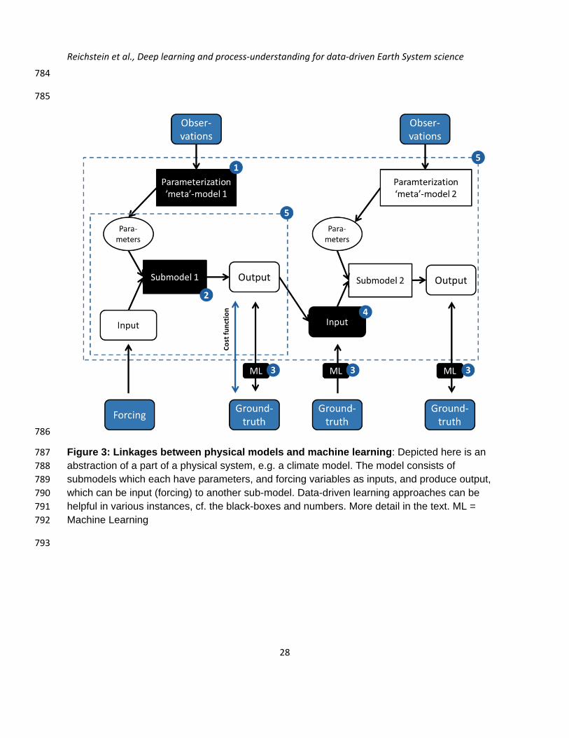
are five points of potential synergy (Figure 3) [the numbers in the following list correspond to the 316
circles in the figure]: 317
1) Improving parameterizations (Fig. 3, linkage 1). Physical models require parameters but 318
many of those cannot be easily derived from first principles. Here, machine learning can learn 319
parameterizations to optimally describe the ground truth which can be observed or generated 320
from detailed and high-resolution models through first principles. For example, instead of 321
assigning parameters of the vegetation in an Earth system model to plant functional types (a 322
common ad hoc decision in most global land surface models), one can allow these 323
parameterizations to be learned from appropriate sets of statistical covariates, allowing them to 324
be more dynamic, interdependent and contextual. A prototypical approach has been taken 325
already in hydrology where the mapping of environmental variables (e.g. precipitation, surface 326
slope) to catchment parameters (e.g. mean, minimum, maximum streamflow) has been learned 327
from a few thousands catchments and applied globally to feed hydrological models63. Another 328
example from global atmospheric modelling is learning the effective coarse-scale physical 329
parameters of precipitating convection (e.g. the fraction of water that is precipitating out of a 330
cloud during convection) from data or high-resolution models64,65.(the high-resolution models are 331
too expensive to run, which is why coarse-scale parametrizations are needed). These learned 332
parametrizations could lead to better representations of tropical convection66,67. 333
2) Replacing a “physical” sub-model with a machine learning model (Fig. 3, linkage 2). If 334
formulations of a submodel are of semi-empirical nature where the functional form has little 335
theoretical basis (e.g. biological processes), this submodel can be replaced by a machine 336
learning model if a sufficient number of observations are available. This leads to a hybrid model, 337
which combines the strengths of physical modeling (theoretical foundations, interpretable 338
compartments) and machine learning (data-adaptiveness). For example, we could couple well 339
established physical (differential) equations of diffusion for transport of water in plants with 340
machine learning for the poorly understood biological regulation of water transport conductance. 341
This results in a more “physical model” that obeys accepted conservation of mass and energy 342
laws, but the regulation (biological) is flexible and learned from data. Such principle has recently 343
been taken to efficiently model motion of water in the ocean and specifically predict sea surface 344
temperatures. Here, the motion field was learned via a deep neural network, and then used to 345
update the heat content and temperatures via physically modelling the movement implied by the 346
motion field68. Also a number of atmospheric scientists have begun experimenting with related 347
Reichstein et al., Deep learning and process-understanding for data-driven Earth System science
12
approaches to circumvent long-standing biases in physically based parameterizations of 348
atmospheric convection65,69. 349
The problem may become more complicated if physical model and machine learning 350
parameters are to be estimated simultaneously while maintaining interpretability, especially 351
when several sub-models are replaced with machine learning approaches. In the field of 352
chemistry this approach has been used in calibration exercises and to describe changes in 353
unknown kinetic rates while maintaining mass balance in biochemical reactors modeling70, 354
which, albeit less complex, bears many similarities to hydrological and biogeochemical 355
modelling. 356
3) Analysis of model-observation mismatch (Fig. 3, linkage 3): Deviations of a physical model 357
from observations can be perceived as imperfect knowledge causing model error, assuming no 358
observational biases. Machine learning can help to identify, visualize and understand the 359
patterns of model error, which allows also to correct model outputs accordingly. For example, 360
machine learning can extract patterns from data automatically and identify those which are not 361
explicitly represented in the physical model. This approach helps improving the physical model 362
and theory. In practice, it can also serve to correct model bias of dynamic variables, or it can 363
facilitate improved downscaling to finer spatial scales compared to tedious and ad hoc hand-364
designed approaches71,72. 365
4) Constraining sub-models (Fig. 3, linkage 4). One can drive a submodel with the output from a 366
machine learning algorithm, instead of another (potentially biased) submodel in an offline 367
simulation. This helps in disentangling model error originating from the submodule of interest 368
from errors of coupled submodules. As a consequence, this simplifies and reduces biases and 369
uncertainties in model parameter calibration or the assimilation of observed system state 370
variables. 371
5) Surrogate modeling or emulation: Emulation of the full (or specific parts of) a physical model 372
can be useful for computational efficiency and tractability reasons. Machine learning emulators 373
once trained can achieve orders of magnitude faster simulations than the original physical 374
model without sacrificing significant accuracy. This allows for fast sensitivity analysis, model 375
parameter calibration, and derivation of confidence intervals for the estimates. For example, 376
machine learning emulators are used to replace computationally expensive, physics-based 377
Reichstein et al., Deep learning and process-understanding for data-driven Earth System science
13
radiative transfer models (RTMs) of the interactions between radiation, vegetation and 378
atmosphere57,73,74 which are critical for the interpretation and assimilation of land surface remote 379
sensing in models. Emulators are also used in dynamic modelling, where states are evolving, 380
e.g. in climate modeling75 and more recently explored in vegetation dynamic models76. Further, 381
given the complexity of physical models, emulation challenges are very good test beds to 382
explore the potential of machine learning and deep learning approaches to extrapolate outside 383
the ranges of training conditions. 384
Some of the concepts in Figure 3 have already been adopted in a broad sense. For instance, 385
point 3) relates to model benchmarking and statistical downscaling and model output 386
statistics77,78. Here we argue that adopting a deep-learning approach will strongly improve the 387
use of spatio-temporal context information for the modification of model output. Emulation (5) 388
has been widely adopted in several branches of engineering and geosciences, mainly for the 389
sake of efficient modelling, but tractability issues have not yet been explored in depth. Other 390
paths, such as the hybrid modelling (Fig. 3, link 2), appear to be much less explored. 391
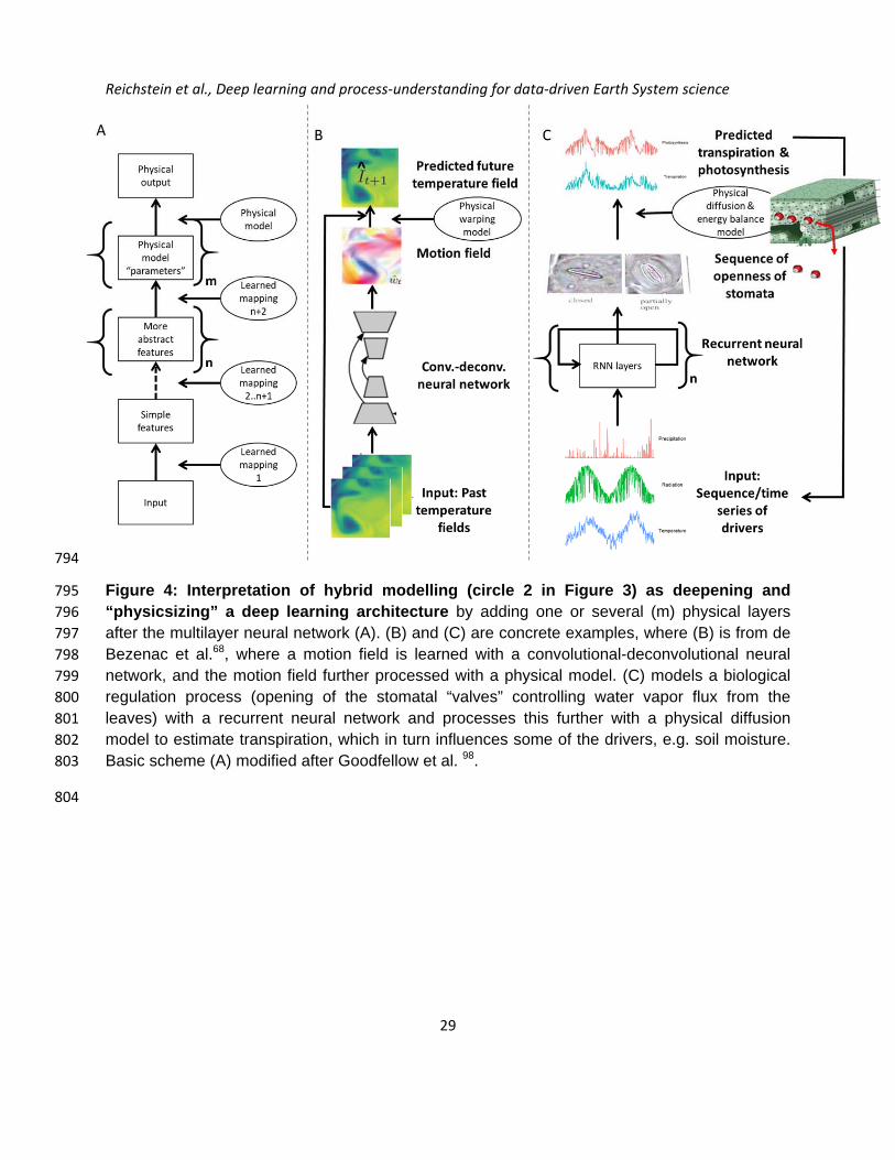
Conceptually the hybrid approaches discussed before can be interpreted as deepening and 392
“physicizing” a neural network (Figure 4), where the physical model comes on top of a neural 393
network layers (see examples Fig. 4b-c). It contrasts the reverse approach discussed above 394
where physical model output is produced and then corrected using additional layers of machine 395
learning approaches. We believe that it is worthwhile pursuing both avenues of integrating 396
physical modelling and machine learning. 397
Figure 3 started from a system-modelling view and seeks to integrate machine learning. As an 398
alternative perspective system knowledge can be integrated into a machine learning framework. 399
This may include respective design of the network architecture36,79, physical constraints in the 400
cost function for optimization58, or expansion of the training data set for under-sampled domains 401
(i.e. physically based data augmentation)80. For instance, while usually a so-called cost-function 402
like ordinary least squares penalizes model-data mismatch, it can be modified to also avoid 403
physically implausible predictions for lake temperature modelling58. The integration of physics 404
and machine learning models may not only achieve improved performance and generalizations 405
but, perhaps more importantly, incorporates consistency and credibility of the machine learning 406
models. As a by-product, the hybridization has an interesting regularization effect as physics 407
discards implausible models. Therefore, physics-aware machine learning models should better 408
combat overfitting, especially in low-to-medium sample sized datasets81. This notion is also 409
Reichstein et al., Deep learning and process-understanding for data-driven Earth System science
14
related to the direction of attaining explainable and interpretable machine learning models 410
(“explainable AI”82), and to combining logic rules with deep neural networks83 411
Recent advancements in two fields of methodological approaches have potential in facilitating 412
the fusion of machine learning and physical models in a sound way: probabilistic 413
programming52, and differentiable programming. Probabilistic programming allows for 414
accounting of various uncertainty aspects in a formal but flexible way. A proper accounting for 415
data and model uncertainty along with integration of knowledge by priors and constraints is 416
critical for optimally combining the data-driven and theory-driven paradigms, including logical 417
rules as done in statistical relational learning. In addition, error propagation is conceptually 418
seamless, facilitating well founded uncertainty margins for model output. This capability is 419
largely missing so far but crucial for scientific purposes, and in particular for management, or 420
policy decisions. Differentiable programming allows for efficient optimization due to automated 421
differentiation84,85. This greatly helps in making the large, non-linear and complex inversion 422
problem computationally more tractable, and in addition allows for explicit sensitivity 423
assessments, thus aiding in interpretability. 424
425
6. Advancing science 426
There is no doubt and there are numerous examples as discussed in this manuscript, that 427
modern machine learning methods significantly improve classification and prediction skills. This 428
alone has great value. Yet, how do they improve fundamental scientific understanding, given 429
that in particular the outcome of complex statistical models remains hard to grasp? The answer 430
can be found in the observations which have virtually always been the basis for scientific 431
progress. The Copernican revolution was possible by precisely observing planetary trajectories 432
to infer and test the laws governing them. While the general cycle of exploration, hypotheses 433
generation and testing remains the same, modern data-driven science and machine learning 434
can extract arbitrarily complex patterns in observational data to challenge complex theories and 435
Earth system models (Supplementary Fig. 3). For instance spatially explicit global data-driven 436
machine learning based estimates of photosynthesis, has indicated an overestimation of 437
photosynthesis in the tropical rainforest by climate models86. This mismatch has led scientists 438
to develop hypotheses that enable a better description of the radiative transfer in vegetation 439
canopies23 which has led to better photosynthesis estimates also in other regions, and better 440
consistency with leaf level observations.. Related data-driven carbon cycle estimates have 441
Reichstein et al., Deep learning and process-understanding for data-driven Earth System science
15
helped calibrating vegetation models and explain the conundrum of the increasing seasonal 442
amplitude of the CO2 concentration in high latitudes87, which according to these results is 443
caused by more vigorous vegetation in the high latitudes. In addition to data-driven theory and 444
model building, extracted patterns are increasingly being used as a way to explore improved 445
parameterizations in Earth system models65,69, and emulators are increasingly being used as a 446
basis for model calibration88. In other words, the scientific interplay between theory and 447
observation, of hypothesis generation and theory-driven hypothesis testing will prevail, but the 448
complexity of hypotheses and tests inferred from data and the pace of this generation are 449
changing by orders of magnitude, implying unprecedented, qualitative and quantitative progress 450
of the science of the complex Earth system. 451
452
7. Conclusion 453 454 Earth sciences face the need to process large and rapidly increasing amounts of data to provide 455
more accurate, less uncertain, and physically consistent inferences in the form of prediction, 456
modeling and understanding the complex Earth system. Machine learning in general, and deep 457
learning in particular, offer promising tools to build new data-driven models for components of 458
the Earth system and thus for understanding of the Earth. The Earth system specific challenges 459
shall further stimulate the development of methodologies, where we have four major 460
recommendations. 461
Recognition of the particularities of the data: multi-source, multi-scale, high dimensional, 462
complex spatial-temporal relations, including non-trivial, and lagged long-distance relationships 463
(teleconnections) between variables need to be adequately modelled. While the deep learning 464
approach is well-positioned to address these data challenges, this may stimulate development 465
of new network architectures, algorithms and approaches, in particular deep-learning 466
approaches which address both spatial and temporal context at different scales (cf. Figure 4). 467
Plausibility and interpretability of inferences: models should not only be accurate but also 468
credible and aware of the physics governing the Earth system. Wide adoption of machine 469
learning in the Earth sciences will be facilitated if models become more transparent and 470
interpretable: their parameters and feature rankings should have a minimal physical 471
Reichstein et al., Deep learning and process-understanding for data-driven Earth System science
16
interpretation, and the model should be reducible/explainable in a set of rules, descriptors, and 472
relations. 473
Uncertainty estimation: Models should speak about their confidence and credibility. A strong 474
integration of Bayesian/probabilistic inference will be an avenue to follow here, because they 475
allow for explicit representation and propagation of uncertainties. In addition, identifying and 476
treating extrapolation is a priority. 477
Testing against complex physical models: the spatial and temporal prediction ability of machine 478
learning should be at least consistent with the patterns observed in physical models. Thus we 479
recommend testing the performance of machine learning methods against synthetic data 480
derived from physical models of the Earth system. For instance, the models in Fig. 4b and c, 481
which are applied to real data, should be tested across a broad range of dynamics as simulated 482
by complex physical models. This is of particular relevance in conditions of limited training data 483
and to assess extrapolation issues. 484
Overall we suggest that future models should integrate process-based and machine learning 485
approaches. Data-driven machine learning approaches to geo-scientific research will not 486
replace physical modelling, but strongly complement and enrich it. Specifically, we envision 487
various synergies between physical and data-driven models, with the ultimate goal of hybrid 488
modelling approaches: they obey physical laws, feature a conceptualized and thus interpretable 489
structure, and at the same time are fully data-adaptive where theory is weak. Importantly, the 490
other way around also holds: machine learning research will benefit from plausible physically 491
based relationships derived from the natural sciences. Among others, two major Earth system 492
challenges resistant to past progress, the parameterization of atmospheric convection and the 493
description of spatio-temporal dependency of ecosystems on climate and interacting geo-494
factors, are open to be addressed with the approaches discussed here. 495
Author information 496
The authors declare no competing interests. 497
Reichstein et al., Deep learning and process-understanding for data-driven Earth System science
17
References 498
1 Howe, L. & Wain, A. Predicting the future. V, 195 p. (Cambridge University Press, 499 1993). 500
2 Bauer, P., Thorpe, A. & Brunet, G. The quiet revolution of numerical weather prediction. 501 Nature 525, 47, doi:10.1038/nature14956 (2015). 502
3 Hantson, S. et al. The status and challenge of global fire modelling. Biogeosciences 13, 503 3359-3375, doi:10.5194/bg-13-3359-2016 (2016). 504
4 Agapiou, A. Remote sensing heritage in a petabyte-scale: satellite data and heritage 505 Earth Engine© applications. Int. J Digit. Earth 10, 85-102 (2017). 506
5 Stockhause, M. & Lautenschlager, M. CMIP6 Data Citation of Evolving Data. Data Sci. J 507 16, doi:10.5334/dsj-2017-030 (2017). 508
6 Lee, J., Weger, R. C., Sengupta, S. K. & Welch, R. M. A neural network approach to 509 cloud classification. IEEE T Geosci. Remote. 28, 846-855, doi:10.1109/36.58972 (1990). 510
7 Benediktsson, J. A., Swain, P. H. & Ersoy, O. K. Neural network approaches versus 511 statistical methods in classification of multisource remote sensing data. IEEE T Geosci. Remote. 512 28, 540-552, doi:10.1109/Tgrs.1990.572944 (1990). 513
8 Camps-Valls, G. & Bruzzone, L. Kernel methods for remote sensing data analysis. 434 514 p. (John Wiley & Sons, 2009). 515
9 Gómez-Chova, L., Tuia, D., Moser, G. & Camps-Valls, G. Multimodal classification of 516 remote sensing images: A review and future directions. P IEEE 103, 1560-1584, 517 doi:10.1109/Jproc.2015.2449668 (2015). 518
10 Camps-Valls, G., Tuia, D., Bruzzone, L. & Benediktsson, J. A. Advances in hyperspectral 519 image classification: Earth monitoring with statistical learning methods. IEEE Signal Proc. 520 Mag. 31, 45-54 (2014). [Comprehensive overview of machine learning for 521 classification] 522
11 Gislason, P. O., Benediktsson, J. A. & Sveinsson, J. R. Random Forests for land cover 523 classification. Pattern Recog. Lett. 27, 294-300, doi:10.1016/j.patrec.2005.08.011 (2006). [One 524 of the first machine learning papers for land cover classification, method now 525 operationally used] 526
12 Muhlbauer, A., McCoy, I. L. & Wood, R. Climatology of stratocumulus cloud 527 morphologies: microphysical properties and radiative effects. Atmos. Chem. Phys. 14, 6695-528 6716, doi:10.5194/acp-14-6695-2014 (2014). 529
Reichstein et al., Deep learning and process-understanding for data-driven Earth System science
18
13 Grimm, R., Behrens, T., Märker, M. & Elsenbeer, H. Soil organic carbon concentrations 530 and stocks on Barro Colorado Island—Digital soil mapping using Random Forests analysis. 531 Geoderma 146, 102-113 (2008). 532
14 Hengl, T. et al. SoilGrids250m: Global gridded soil information based on machine 533 learning. PLoS One 12, e0169748, doi:10.1371/journal.pone.0169748 (2017). [Machine 534 learning used for operational global soil mapping] 535
15 Townsend, P. A., Foster, J. R., Chastain, R. A. & Currie, W. S. Application of imaging 536 spectroscopy to mapping canopy nitrogen in the forests of the central Appalachian Mountains 537 using Hyperion and AVIRIS. IEEE T Geosci. Remote. 41, 1347-1354, 538 doi:10.1109/Tgrs.2003.813205 (2003). 539
16 Coops, N. C., Smith, M.-L., Martin, M. E. & Ollinger, S. V. Prediction of eucalypt foliage 540 nitrogen content from satellite-derived hyperspectral data. IEEE T Geosci. Remote. 41, 1338-541 1346, doi:10.1109/Tgrs.2003.813135 (2003). 542
17 Verrelst, J., Alonso, L., Camps-Valls, G., Delegido, J. & Moreno, J. Retrieval of 543 vegetation biophysical parameters using Gaussian process techniques. IEEE T Geosci. 544 Remote. 50, 1832-1843, doi:10.1109/Tgrs.2011.2168962 (2012). 545
18 Papale, D. & Valentini, R. A new assessment of European forests carbon exchanges by 546 eddy fluxes and artificial neural network spatialization. Global Change Biol. 9, 525-535, 547 doi:10.1046/j.1365-2486.2003.00609.x (2003). 548
19 Jung, M. et al. Global patterns of land-atmosphere fluxes of carbon dioxide, latent heat, 549 and sensible heat derived from eddy covariance, satellite, and meteorological observations. J 550 Geophys. Res. - Biogeo. 116, G00j07, doi:10.1029/2010jg001566 (2011). 551
20 Tramontana, G. et al. Predicting carbon dioxide and energy fluxes across global 552 FLUXNET sites with regression algorithms. Biogeosciences 13, 4291 - 4313, doi:10.5194/bg-553 13-4291-2016 (2016). 554
21 Jung, M. et al. Recent decline in the global land evapotranspiration trend due to limited 555 moisture supply. Nature 467, 951 - 954, doi:10.1038/nature09396 (2010). [First data-556 driven machine learning based spatio-temporal estimation of global water fluxes on 557 land] 558
559
22 Jung, M. et al. Compensatory water effects link yearly global land CO2 sink changes to 560 temperature. Nature 541, 516 - 520, doi:10.1038/nature20780 (2017). 561
23 Bonan, G. B. et al. Improving canopy processes in the Community Land Model version 4 562 (CLM4) using global flux fields empirically inferred from FLUXNET data. J Geophys. Res. - 563 Biogeo. 116, G02014, doi:10.1029/2010jg001593 (2011). 564
Reichstein et al., Deep learning and process-understanding for data-driven Earth System science
19
24 Anav, A. et al. Spatiotemporal patterns of terrestrial gross primary production: A review. 565 Rev. Geophys. 53, 785-818, doi:10.1002/2015rg000483 (2015). 566
25 Landschützer, P. et al. A neural network-based estimate of the seasonal to inter-annual 567 variability of the Atlantic Ocean carbon sink. Biogeosciences 10, 7793-7815, doi:10.5194/bg-10-568 7793-2013 (2013). [First data-driven machine learning based carbon fluxes in the ocean] 569
26 Kühnlein, M., Appelhans, T., Thies, B. & Nauss, T. Improving the accuracy of rainfall 570 rates from optical satellite sensors with machine learning—A random forests-based approach 571 applied to MSG SEVIRI. Remote Sens. Environ. 141, 129-143 (2014). 572
27 Caldwell, P. M. et al. Statistical significance of climate sensitivity predictors obtained by 573 data mining. Geophys. Res. Lett. 41, 1803-1808, doi:10.1002/2014gl059205 (2014). 574
28 Reichstein, M. & Beer, C. Soil respiration across scales: the importance of a model-data 575 integration framework for data interpretation. J. Plant Nutr. Soil Sci. 171, 344 - 354, 576 doi:10.1002/jpln.200700075 (2008). 577
29 Wright, S. Correlation and causation. J. Agric. Res. 20, 557-585 (1921). 578
30 Guttman, N. B. Accepting the standardized precipitation index: a calculation algorithm. J 579 Am. Water. Resour. As. 35, 311-322, doi:10.1111/j.1752-1688.1999.tb03592.x (1999). 580
31 Vicente-Serrano, S. M., Beguería, S. & López-Moreno, J. I. A multiscalar drought index 581 sensitive to global warming: the standardized precipitation evapotranspiration index. J. Clim. 23, 582 1696-1718, doi:10.1175/2009jcli2909.1 (2010). 583
32 LeCun, Y., Bengio, Y. & Hinton, G. Deep learning. Nature 521, 436-444, 584 doi:10.1038/nature14539 (2015). 585
33 Lore, K. G., Stoecklein, D., Davies, M., Ganapathysubramanian, B. & Sarkar, S. in 586 JMLR: Workshop and Conference Proceeding / The 1st International Workshop “Feature 587 Extraction: Modern Questions and Challenge" Vol. 44 213-225 (Montreal, Canada, 2015). 588
34 Baldi, P., Sadowski, P. & Whiteson, D. Searching for exotic particles in high-energy 589 physics with deep learning. Nat. Commun. 5, 4308, doi:10.1038/ncomms5308 (2014). 590
35 Bhimji, W., Farrell, S. A., Kurth, T., Paganini, M. & Racah, E. Deep Neural Networks for 591 Physics Analysis on low-level whole-detector data at the LHC. arXiv.org e-Print archive, 592 arXiv:1711.03573 (2017). 593
36 Schutt, K. T., Arbabzadah, F., Chmiela, S., Muller, K. R. & Tkatchenko, A. Quantum-594 chemical insights from deep tensor neural networks. Nat. Commun. 8, 13890, 595 doi:10.1038/ncomms13890 (2017). 596
Reichstein et al., Deep learning and process-understanding for data-driven Earth System science
20
37 Alipanahi, B., Delong, A., Weirauch, M. T. & Frey, B. J. Predicting the sequence 597 specificities of DNA-and RNA-binding proteins by deep learning. Nat. Biotechnol. 33, 831-838, 598 doi:10.1038/nbt.3300 (2015). 599
38 Prabhat. A Look at Deep Learning for Science, O’Reilly Blog., 600 https://www.oreilly.com/ideas/a-look-at-deep-learning-for-science (2017). 601
39 Zhang, L. P., Zhang, L. F. & Du, B. Deep Learning for Remote Sensing Data A technical 602 tutorial on the state of the art. IEEE Geosc. Rem. Sen. M 4, 22-40, 603 doi:10.1109/Mgrs.2016.2540798 (2016). 604
40 Ball, J. E., Anderson, D. T. & Chan, C. S. Comprehensive survey of deep learning in 605 remote sensing: theories, tools, and challenges for the community. J Appl. Remote Sens. 11, 606 042609, doi:10.1117/1.Jrs.11.042609 (2017). 607
41 Racah, E. et al. ExtremeWeather: A large-scale climate dataset for semi-supervised 608 detection, localization, and understanding of extreme weather events. Adv. Neural. Inf. Process. 609 Syst., 3405-3416 (2017). 610
42 Liu, Y. et al. in ABDA'16 - Internationall Conference on Advances in Big Data Analytics 611 81-88 (2016). [First approach to automatically detect extreme weather without any 612 prescribed thresholds, using deep learning] 613
43 Zhao, W. Z. & Du, S. H. Learning multiscale and deep representations for classifying 614 remotely sensed imagery. ISPRS J Photogramm. Remote. Sens. 113, 155-165, 615 doi:10.1016/j.isprsjprs.2016.01.004 (2016). 616
44 Mathieu, M., Couprie, C. & LeCun, Y. Deep multi-scale video prediction beyond mean 617 square error. arXiv.org e-Print archive, arXiv:1511.05440 (2015). 618
45 Oh, J., Guo, X., Lee, H., Lewis, R. L. & Singh, S. Action-conditional video prediction 619 using deep networks in atari games. Adv. Neural. Inf. Process. Syst., 2863-2871 (2015). 620
46 Shi, X. et al. Convolutional LSTM Network: A Machine Learning Approach for 621 Precipitation Nowcasting. Adv. Neural. Inf. Process. Syst. 28, 802-810 (2015). 622
47 Deng, J. et al. in 2009 IEEE Conference on Computer Vision and Pattern Recognition 623 248-255 (IEEE, Miami, FL, 2009). 624
48 Friedlingstein, P. et al. Uncertainties in CMIP5 Climate Projections due to Carbon Cycle 625 Feedbacks. J. Clim. 27, 511-526, doi:10.1175/jcli-d-12-00579.1 (2014). 626
49 Montavon, G., Samek, W. & Müller, K.-R. Methods for interpreting and understanding 627 deep neural networks. Digit. Signal Process. (2017). 628
Reichstein et al., Deep learning and process-understanding for data-driven Earth System science
21
50 Runge, J. et al. Identifying causal gateways and mediators in complex spatio-temporal 629 systems. Nat. Commun. 6, 8502, doi:10.1038/ncomms9502 (2015). 630
51 Chalupka, K., Bischoff, T., Perona, P. & Eberhardt, F. in UAI'16 Proceedings of the 631 Thirty-Second Conference on Uncertainty in Artificial Intelligence 72-81 (AUAI Press Arlington, 632 Jersey City, New Jersey, USA, 2016). 633
52 Ghahramani, Z. Probabilistic machine learning and artificial intelligence. Nature 521, 634 452, doi:10.1038/nature14541 (2015). 635
53 Goodfellow, I. J. et al. Generative Adversarial Nets. Adv. Neural. Inf. Process. Syst. 27, 636 2672-2680 (2014). [Fundamental paper on a deep generative modelling approach, 637 allowing one to model e.g. possible futures from data] 638
54 Hansen, M. C. et al. High-resolution global maps of 21st-century forest cover change. 639 Science 342, 850-853, doi:10.1126/science.1244693 (2013). 640
55 Pekel, J.-F., Cottam, A., Gorelick, N. & Belward, A. S. High-resolution mapping of global 641 surface water and its long-term changes. Nature 540, 418-422, doi:10.1038/nature20584 642 (2016). 643
56 Karpatne, A. et al. Theory-guided Data Science: A New Paradigm for Scientific 644 Discovery from Data. IEEE T Knowl. Data En. 29, 2318-2331, doi:10.1109/TKDE.2017.2720168 645 (2017). 646
57 Camps-Valls, G. et al. Physics-aware Gaussian processes in remote sensing. Appl. Soft 647 Comput. 68, 69-82, doi:10.1016/j.asoc.2018.03.021 (2018). 648
58 Karpatne, A., Watkins, W., Read, J. & Kumar, V. Physics-guided Neural Networks 649 (PGNN): An Application in Lake Temperature Modeling. arXiv.org e-Print archive, 650 arXiv:1710.11431 (2017). 651
59 Luo, Y. Q. et al. A framework for benchmarking land models. Biogeosciences 9, 3857 - 652 3874, doi:10.5194/bg-9-3857-2012 (2012). 653
60 Eyring, V. et al. Towards improved and more routine Earth system model evaluation in 654 CMIP. Earth Syst. Dynam. 7, 813-830, doi:10.5194/esd-7-813-2016 (2016). 655
61 Klocke, D., Pincus, R. & Quaas, J. On constraining estimates of climate sensitivity with 656 present-day observations through model weighting. J. Clim. 24, 6092-6099, 657 doi:10.1175/2011jcli4193.1 (2011). 658
62 Cox, P. M. et al. Sensitivity of tropical carbon to climate change constrained by carbon 659 dioxide variability. Nature 494, 341-344, doi:10.1038/nature11882 (2013). 660
Reichstein et al., Deep learning and process-understanding for data-driven Earth System science
22
63 Beck, H. E. et al. Global‐scale regionalization of hydrologic model parameters. Water 661 Resour. Res. 52, 3599-3622 (2016). 662
64 Schirber, S., Klocke, D., Pincus, R., Quaas, J. & Anderson, J. L. Parameter estimation 663 using data assimilation in an atmospheric general circulation model: From a perfect toward the 664 real world. J Adv. Model. Earth Systems 5, 58-70, doi:10.1029/2012ms000167 (2013). 665
65 Gentine, P., Pritchard, M., Rasp, S., Reinaudi, G. & Yacalis, G. Could machine learning 666 break the convection parameterization deadlock? Geophys. Res. Lett. 45, 5742–5751, 667 doi:10.1029/2018GL078202 (2018). 668
66 Becker, T., Stevens, B. & Hohenegger, C. Imprint of the convective parameterization 669 and sea‐surface temperature on large‐scale convective self‐aggregation. J Adv. Model. Earth 670 Systems (2017). 671
67 Siongco, A. C., Hohenegger, C. & Stevens, B. Sensitivity of the summertime tropical 672 Atlantic precipitation distribution to convective parameterization and model resolution in 673 ECHAM6. J Geophys. Res. - Atmos. 122, 2579-2594, doi:10.1002/2016jd026093 (2017). 674
68 de Bezenac, E., Pajot, A. & Gallinari, P. Deep Learning for Physical Processes: 675 Incorporating Prior Scientific Knowledge. arXiv.org e-Print archive, arXiv:1711.07970 (2017). 676
69 Brenowitz, N. D. & Bretherton, C. S. Prognostic validation of a neural network unified 677 physics parameterization. Geophys. Res. Lett. 45, 6289-6298, doi:10.1029/2018gl078510 678 (2018). 679
70 Willis, M. J. & von Stosch, M. Simultaneous parameter identification and discrimination 680 of the nonparametric structure of hybrid semi-parametric models. Comput. Chem. Eng. 104, 681 366-376, doi:10.1016/j.compchemeng.2017.05.005 (2017). 682
71 McGovern, A. et al. Using artificial intelligence to improve real-time decision making for 683 high-impact weather. B Am. Meteorol. Soc. 98, 2073-2090, doi:10.1175/Bams-D-16-0123.1 684 (2017). 685
72 Vandal, T. et al. in Proceedings of the Twenty-Seventh International Joint Conference on 686 Artificial Intelligence (IJCAI-18) 5389-5393 (Stockholm, Sweden, 2018). 687
73 Verrelst, J. et al. Emulation of Leaf, Canopy and Atmosphere Radiative Transfer Models 688 for Fast Global Sensitivity Analysis. Remote Sens. 8, 673, doi:10.3390/rs8080673 (2016). 689
74 Chevallier, F., Chéruy, F., Scott, N. & Chédin, A. A neural network approach for a fast 690 and accurate computation of a longwave radiative budget. J Appl. Meteorol. 37, 1385-1397, 691 doi:10.1175/1520-0450(1998)037<1385:Annafa>2.0.Co;2 (1998). 692
75 Castruccio, S. et al. Statistical emulation of climate model projections based on 693 precomputed GCM runs. J. Clim. 27, 1829-1844, doi:10.1175/Jcli-D-13-00099.1 (2014). 694
Reichstein et al., Deep learning and process-understanding for data-driven Earth System science
23
76 Fer, I. et al. Linking big models to big data: efficient ecosystem model calibration through 695 Bayesian model emulation. Biogeosci. Disc. 2018, 1-30, doi:10.5194/bg-2018-96 (2018). 696
77 Glahn, H. R. & Lowry, D. A. The use of model output statistics (MOS) in objective 697 weather forecasting. J Appl. Meteorol. 11, 1203-1211 (1972). 698
78 Wilks, D. S. Multivariate ensemble Model Output Statistics using empirical copulas. Q J 699 Roy. Meteor. Soc. 141, 945-952, doi:10.1002/qj.2414 (2015). 700
79 Tewari, A. et al. in Proceedings of the IEEE Conference on Computer Vision and Pattern 701 Recognition 2549-2559 (2018). 702
80 Xie, Y., Franz, E., Chu, M. & Thuerey, N. tempoGAN: A Temporally Coherent, 703 Volumetric GAN for Super-resolution Fluid Flow. arXiv.org e-Print archive, arXiv:1801.09710 704 (2018). 705
81 Stewart, R. & Ermon, S. in Proceedings of the Thirty-First AAAI Conference on Artificial 706 Intelligence (AAAI-17) 2576-2582 (San Francisco, California USA, 2017). 707
82 Gunning, D. Explainable artificial intelligence (xai), 708 https://www.cc.gatech.edu/~alanwags/DLAI2016/(Gunning)%20IJCAI-16%20DLAI%20WS.pdf 709 (2017). 710
83 Hu, Z., Ma, X., Liu, Z., Hovy, E. & Xing, E. in Proceedings of the 54th Annual Meeting of 711 the Association for Computational Linguistics Vol. 1: Long Papers 2410–2420 (Association for 712 Computational Linguistics, 2016). 713
84 Pearlmutter, B. A. & Siskind, J. M. Reverse-mode AD in a functional framework: Lambda 714 the ultimate backpropagator. ACM T Progr. Lang. Sys. 30, 7, doi:10.1145/1330017.1330018 715 (2008). 716
85 Wang, F. & Rompf, T. in ICLR 2018 Workshop (2018). 717
86 Beer, C. et al. Terrestrial Gross Carbon Dioxide Uptake: Global Distribution and 718 Covariation with Climate. Science 329, 834 - 838, doi:10.1126/science.1184984 (2010). 719
87 Forkel, M. et al. Enhanced seasonal CO2 exchange caused by amplified plant 720 productivity in northern ecosystems. Science 351, 696-699, doi:10.1126/science.aac4971 721 (2016). 722
88 Bellprat, O., Kotlarski, S., Lüthi, D. & Schär, C. Objective calibration of regional climate 723 models. J Geophys. Res. - Atmos. 117, D23115, doi:10.1029/2012jd018262 (2012). 724
89 Reichstein, M. et al. in AGU Fall Meeting Abstracts 2016AGUFM.B2044A..2007R 725 (2016). 726
Reichstein et al., Deep learning and process-understanding for data-driven Earth System science
24
90 Rußwurm, M. & Körner, M. Multi-temporal land cover classification with long short-term 727 memory neural networks. Int. Arch. Photogramm. Remote Sens. Spatial Inf. Sci. XLII-1/W1, 728 551-558, doi:10.5194/isprs-archives-XLII-1-W1-551-2017 (2017). [First Use of LSTM deep 729 learning model for multi-temporal land-cover classification] 730
91 Nash, J. E. & Sutcliffe, J. V. River flow forecasting through conceptual models part I—A 731 discussion of principles. J Hydrol. 10, 282-290 (1970). 732
92 Shi, X. et al. Deep Learning for Precipitation Nowcasting: A Benchmark and A New 733 Model. Adv. Neural. Inf. Process. Syst. 30, 5617-5627 (2017). [First approach to data-driven 734 modelling of near-term precipitation using a combination of deep-learning concepts, i.e. 735 LSTMs and convolutional neural networks] 736
93 Isola, P., Zhu, J.-Y., Zhou, T. & Efros, A. A. Image-to-image translation with conditional 737 adversarial networks. arXiv.org e-Print archive, arXiv:1611.07004v07001 (2016). [A geo-738 science related extension application of Goodfellow et al., where e.g. remote sensing 739 images are transferred to thematic maps] 740
94 Tompson, J., Schlachter, K., Sprechmann, P. & Perlin, K. in Proceedings of the 34th 741 International Conference on Machine Learning Vol. 70 (eds Doina Precup & Yee Whye Teh) 742 3424-3433 (PMLR, Proceedings of Machine Learning Research, 2017). 743
95 https://nar.ucar.edu/2013/ral/short-term-explicit-prediction-step-program 744
96 Ren, S., He, K., Girshick, R. & Sun, J. Faster R-CNN: Towards real-time object detection 745 with region proposal networks. Adv. Neural. Inf. Process. Syst., 91-99 (2015). 746
97 Zaytar, M. A. & El Amrani, C. Sequence to sequence weather forecasting with long short 747 term memory recurrent neural networks. Int. J Comput. Appl. 143 (2016). 748
98 Goodfellow, I., Bengio, Y. & Courville, A. Deep learning. xxii, 775 p. (MIT press, 2016). 749
99 May, R. M. Simple mathematical models with very complicated dynamics. Nature 261, 750 459-467, doi:10.1038/261459a0 (1976). 751
100 Siegelmann, H. T. & Sontag, E. D. On the computational power of neural nets. J 752 Comput. Syst. Sci. 50, 132-150, doi:10.1006/jcss.1995.1013 (1995). 753
101 Hochreiter, S. & Schmidhuber, J. Long short-term memory. Neural Comput. 9, 1735-754 1780 (1997). 755
102 Schmidhuber, J. Deep learning in neural networks: An overview. Neural Netw. 61, 85-756 117, doi:10.1016/j.neunet.2014.09.003 (2015). 757
758
Reichstein et al., Deep learning and process-understanding for data-driven Earth System science
25
Tables 759
760
Table 1: Geoscientific tasks, conventional approaches, their limitations and potential of deep 761 learning approaches 762
Analytical Task Scientific Task Conventional approaches
Limitations Emergent or potential approaches
Classification and anomaly detection
Finding extreme weather patterns
Multivariate, threshold based detection
Heuristic approach, ad hoc criteria used
Supervised and Semi-supervised Convolutional Neural Networks41,42
Land-use and change detection
Pixel-by-pixel spectral classification
No or only shallow spatial context used
Convolutional Neural Networks43
Regression Predict fluxes
from atmospheric conditions
Random forests Kernel methods Feedforward NNs
Memory and lag effects not considered
Recurrent neural networks, LSTMs 89
Predict vegetation properties from atmospheric conditions
Semi-empirical algorithms (temperature sums, water deficits)
Prescriptive in terms of functional forms and dynamic assumptions
Recurrent neural networks90, possibly with spatial context
Predict river runoff in ungauged catchments
Process-models or statistical models with hand-designed topographic features91
Consideration of spatial context limited to hand-designed features
Combination of convolutional neural network with recurrent networks
State Prediction
Precipitation nowcasting
Physical modelling with data-assimilation
Computational limits due to resolution, data only used to update states
Convolutional-LSTM nets short-range spatial context92
Downscaling and bias correcting forecasts
Dynamic modelling and statistical approaches
Computational limits; subjective feature selection
Convolutional nets 72, cGANs53,93
Seasonal forecasts
Physical modelling with initial conditions from data
Fully dependent on physical model, current skill relatively weak
Convolutional-LSTM nets with long-range spatial context
Transport modelling
Physical modelling of transport
Fully dependent on physical model, computational limits
Hybrid physical-convolutional network models94,68
763
Reichstein et al., Deep learning and process-understanding for data-driven Earth System science
26
764
765
766
Figures with captions 767
768
769
770 771
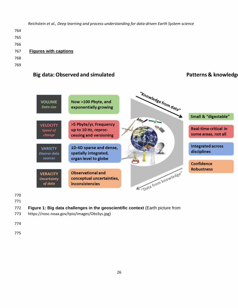
Figure 1: Big data challenges in the geoscientific context (Earth picture from 772 https://nosc.noaa.gov/tpio/images/ObsSys.jpg) 773
774
775
Reichstein et al., Deep learning and process-understanding for data-driven Earth System science
27
776
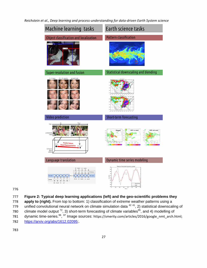
Figure 2: Typical deep learning applications (left) and the geo-scientific problems they 777 apply to (right). From top to bottom: 1) classification of extreme weather patterns using a 778 unified convolutional neural network on climate simulation data 42 41, 2) statistical downscaling of 779 climate model output 72, 3) short-term forecasting of climate variables95, and 4) modelling of 780 dynamic time-series.96, 97 Image sources: https://smerity.com/articles/2016/google_nmt_arch.html; 781 https://arxiv.org/abs/1612.02095;. 782
783
Reichstein et al., Deep learning and process-understanding for data-driven Earth System science
28
784
785
786
Figure 3: Linkages between physical models and machine learning: Depicted here is an 787 abstraction of a part of a physical system, e.g. a climate model. The model consists of 788 submodels which each have parameters, and forcing variables as inputs, and produce output, 789 which can be input (forcing) to another sub-model. Data-driven learning approaches can be 790 helpful in various instances, cf. the black-boxes and numbers. More detail in the text. ML = 791 Machine Learning 792
793
Reichstein et al., Deep learning and process-understanding for data-driven Earth System science
29
794
Figure 4: Interpretation of hybrid modelling (circle 2 in Figure 3) as deepening and 795 “physicsizing” a deep learning architecture by adding one or several (m) physical layers 796 after the multilayer neural network (A). (B) and (C) are concrete examples, where (B) is from de 797 Bezenac et al.68, where a motion field is learned with a convolutional-deconvolutional neural 798 network, and the motion field further processed with a physical model. (C) models a biological 799 regulation process (opening of the stomatal “valves” controlling water vapor flux from the 800 leaves) with a recurrent neural network and processes this further with a physical diffusion 801 model to estimate transpiration, which in turn influences some of the drivers, e.g. soil moisture. 802 Basic scheme (A) modified after Goodfellow et al. 98. 803
804
Reichstein et al., Deep learning and process-understanding for data-driven Earth System science
30
Supplementary material and glossary 805
Efficient modelling a dynamic non-linear system with recurrent neural networks 806
Aforementioned state-of-the-art examples of mapping sequences of driving variables (e.g. 807 meteorological conditions) onto target variables such as CO2 fluxes from ocean or land have considered 808 instantaneous mapping without representation of state dynamics. Dynamic effects have either been 809 considered by directly using observed states as predictors (e.g. vegetation state represented by 810 reflectance) or by introducing hand-designed features. The general problem is depicted in the figure 811 below, where the input acts on an unknown, unobservable system state, while the observable is both 812 influenced by the past state and the current input. It is not a problem of forecasting a time series a few 813 steps ahead, because the whole output sequence has to be predicted by the model. 814
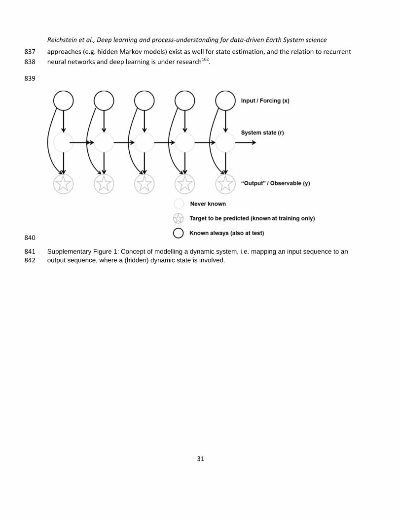
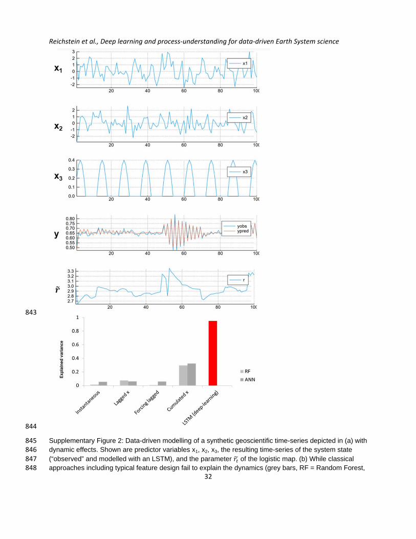
As an example, in the synthetic dynamic system below (one realization in Figure Box 1) we have three 815 forcing variables x1, x2, x3 where two of them influence one (unobserved) state r according to 816 = , , , , ,with 817
, , , , = ∙ , ∙ , ∙ , + (1 − ) ∙ , 818
τ being a parameter determining the inertia of the dynamics of r, here set to 0.05. A target state y to be 819 predicted evolves as a logistic map well known from ecology and chaos theory99: 820 = ∙ ∙ (1 − ), 821
where (contrary to the standard logistic map) the parameter is not fixed but dynamic and dependent 822 on r as 823 = ( + , ), 824
where g simply scales onto the interval [2.5, 4] which implies dynamics varying with time between 825 dampened oscillations, limit cycles and chaos. In the synthetic example 500 realizations of x1 and x2 as 826 Gaussian i.i.d. variables are generated, while x3 is always a seasonal variable as in the Figure below. 827 Obviously x1 and x2 are mimicking a stochastic forcing, whereas x3 represents a deterministic forcing 828 (e.g. solar radiation varying diurnally and seasonally). 829
The lower panel shows the performance of different approaches to model the sequence given the 830 sequences of … . With a feed-forward ANN or random forests it is hard to model the sequence , 831 even with including intuitive features which represent lagged or memory effects, such as lagged or 832 cumulated x variables over the last 25 time steps. On the contrary, being turing-complete100 a recurrent 833 NN has the potential to describe any dynamic system, and the challenge is the parameter estimation or 834 training. In the specific case a simple LSTM101 with 8 cells was trained on 80% of the realizations and the 835 results are shown here for the test set. Certainly, other modelling approaches such as dynamic Bayesian 836
Reichstein et al., Deep learning and process-understanding for data-driven Earth System science
31
approaches (e.g. hidden Markov models) exist as well for state estimation, and the relation to recurrent 837 neural networks and deep learning is under research102. 838
839
840
Supplementary Figure 1: Concept of modelling a dynamic system, i.e. mapping an input sequence to an 841 output sequence, where a (hidden) dynamic state is involved. 842
Reichstein et al., Deep learning and process-understanding for data-driven Earth System science
32
843
844
Supplementary Figure 2: Data-driven modelling of a synthetic geoscientific time-series depicted in (a) with 845 dynamic effects. Shown are predictor variables x1, x2, x3, the resulting time-series of the system state 846 (“observed” and modelled with an LSTM), and the parameter of the logistic map. (b) While classical 847 approaches including typical feature design fail to explain the dynamics (grey bars, RF = Random Forest, 848
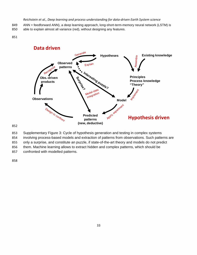
Reichstein et al., Deep learning and process-understanding for data-driven Earth System science
33
ANN = feedforward ANN), a deep learning approach, long-short-term-memory neural network (LSTM) is 849 able to explain almost all variance (red), without designing any features. 850
851
852
Supplementary Figure 3: Cycle of hypothesis generation and testing in complex systems 853 involving process-based models and extraction of patterns from observations. Such patterns are 854 only a surprise, and constitute an puzzle, if state-of-the-art theory and models do not predict 855 them. Machine learning allows to extract hidden and complex patterns, which should be 856 confronted with modelled patterns. 857
858
Observed patterns
Obs.-drivenproducts
Hypotheses
PrinciplesProcess knowledge“Theory”
Model
Existing knowledge
Observations
Predictedpatterns
(new, deductive)
Data driven
Hypothesis driven
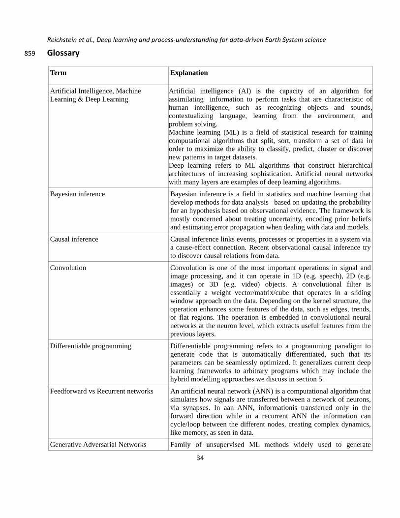
Reichstein et al., Deep learning and process-understanding for data-driven Earth System science
34
Glossary 859
Term Explanation
Artificial Intelligence, Machine Learning & Deep Learning
Artificial intelligence (AI) is the capacity of an algorithm for assimilating information to perform tasks that are characteristic of human intelligence, such as recognizing objects and sounds, contextualizing language, learning from the environment, and problem solving. Machine learning (ML) is a field of statistical research for training computational algorithms that split, sort, transform a set of data in order to maximize the ability to classify, predict, cluster or discover new patterns in target datasets. Deep learning refers to ML algorithms that construct hierarchical architectures of increasing sophistication. Artificial neural networks with many layers are examples of deep learning algorithms.
Bayesian inference Bayesian inference is a field in statistics and machine learning that develop methods for data analysis based on updating the probability for an hypothesis based on observational evidence. The framework is mostly concerned about treating uncertainty, encoding prior beliefs and estimating error propagation when dealing with data and models.
Causal inference Causal inference links events, processes or properties in a system via a cause-effect connection. Recent observational causal inference try to discover causal relations from data.
Convolution Convolution is one of the most important operations in signal and image processing, and it can operate in 1D (e.g. speech), 2D (e.g. images) or 3D (e.g. video) objects. A convolutional filter is essentially a weight vector/matrix/cube that operates in a sliding window approach on the data. Depending on the kernel structure, the operation enhances some features of the data, such as edges, trends, or flat regions. The operation is embedded in convolutional neural networks at the neuron level, which extracts useful features from the previous layers.
Differentiable programming Differentiable programming refers to a programming paradigm to generate code that is automatically differentiated, such that its parameters can be seamlessly optimized. It generalizes current deep learning frameworks to arbitrary programs which may include the hybrid modelling approaches we discuss in section 5.
Feedforward vs Recurrent networks An artificial neural network (ANN) is a computational algorithm that simulates how signals are transferred between a network of neurons, via synapses. In aan ANN, informationis transferred only in the forward direction while in a recurrent ANN the information can cycle/loop between the different nodes, creating complex dynamics, like memory, as seen in data.
Generative Adversarial Networks Family of unsupervised ML methods widely used to generate
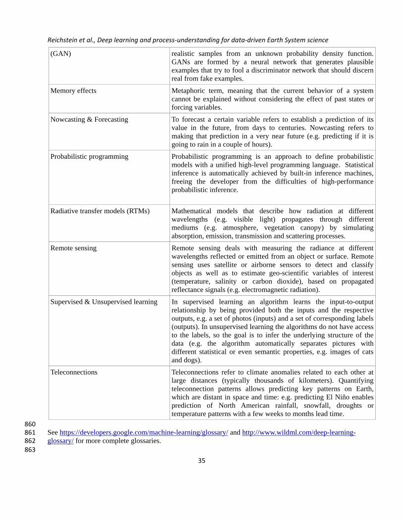
Reichstein et al., Deep learning and process-understanding for data-driven Earth System science
35
(GAN) realistic samples from an unknown probability density function. GANs are formed by a neural network that generates plausible examples that try to fool a discriminator network that should discern real from fake examples.
Memory effects Metaphoric term, meaning that the current behavior of a system cannot be explained without considering the effect of past states or forcing variables.
Nowcasting & Forecasting To forecast a certain variable refers to establish a prediction of its value in the future, from days to centuries. Nowcasting refers to making that prediction in a very near future (e.g. predicting if it is going to rain in a couple of hours).
Probabilistic programming Probabilistic programming is an approach to define probabilistic models with a unified high-level programming language. Statistical inference is automatically achieved by built-in inference machines, freeing the developer from the difficulties of high-performance probabilistic inference.
Radiative transfer models (RTMs) Mathematical models that describe how radiation at different wavelengths (e.g. visible light) propagates through different mediums (e.g. atmosphere, vegetation canopy) by simulating absorption, emission, transmission and scattering processes.
Remote sensing Remote sensing deals with measuring the radiance at different wavelengths reflected or emitted from an object or surface. Remote sensing uses satellite or airborne sensors to detect and classify objects as well as to estimate geo-scientific variables of interest (temperature, salinity or carbon dioxide), based on propagated reflectance signals (e.g. electromagnetic radiation).
Supervised & Unsupervised learning In supervised learning an algorithm learns the input-to-output relationship by being provided both the inputs and the respective outputs, e.g. a set of photos (inputs) and a set of corresponding labels (outputs). In unsupervised learning the algorithms do not have access to the labels, so the goal is to infer the underlying structure of the data (e.g. the algorithm automatically separates pictures with different statistical or even semantic properties, e.g. images of cats and dogs).
Teleconnections Teleconnections refer to climate anomalies related to each other at large distances (typically thousands of kilometers). Quantifying teleconnection patterns allows predicting key patterns on Earth, which are distant in space and time: e.g. predicting El Niño enables prediction of North American rainfall, snowfall, droughts or temperature patterns with a few weeks to months lead time.
860 See https://developers.google.com/machine-learning/glossary/ and http://www.wildml.com/deep-learning-861 glossary/ for more complete glossaries. 862 863

Reichstein et al., Deep learning and process-understanding for data-driven Earth System science
36
864
865