Getting Handcuffs on an Octopus: Minimum Wages, Employment and Turnover

Kaj Gittings Louisiana State University

Texas Tech University – January 2013

Comment by Martin Baily (1982, NBER):

“Trying to understand the nature of unemployment is like trying to handcuff and octopus. You think you have it tied down and then another pair of tentacles get you around the throat.”

Let’s Handcuff An Octopus

• The effect of minimum wages on employment has been investigated for decades, although there is little consensus even today

• This research is unique in that it places the minimum wage debate in a dynamic framework

• Completely new insights into: – How workers and jobs are reallocated – The role worker turnover plays in mediating disemployment effects – How minimum wages affect job stability – Implications for the duration of unemployment (Eurosclerosis)

• These results help explain previously puzzling empirical findings that

minimum wages have very little or not effect on employment

• We also introduce a new used data set emphasizing labor market dynamics (QWI)

Related Literature

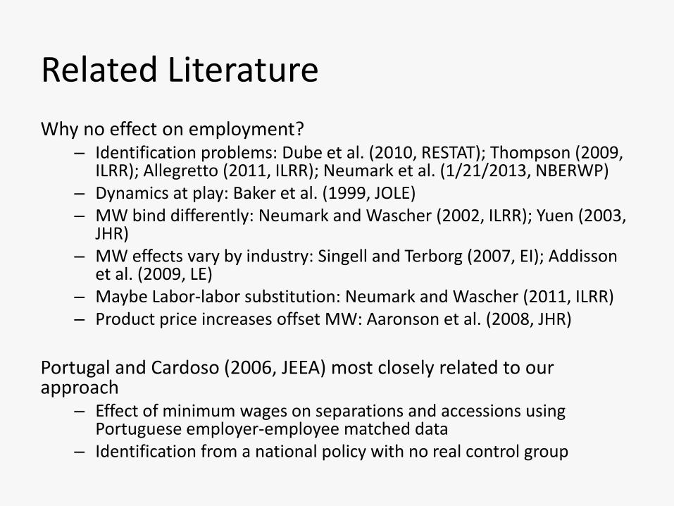
Why no effect on employment? – Identification problems: Dube et al. (2010, RESTAT); Thompson (2009,

ILRR); Allegretto (2011, ILRR); Neumark et al. (1/21/2013, NBERWP) – Dynamics at play: Baker et al. (1999, JOLE) – MW bind differently: Neumark and Wascher (2002, ILRR); Yuen (2003,

JHR) – MW effects vary by industry: Singell and Terborg (2007, EI); Addisson

et al. (2009, LE) – Maybe Labor-labor substitution: Neumark and Wascher (2011, ILRR) – Product price increases offset MW: Aaronson et al. (2008, JHR)

Portugal and Cardoso (2006, JEEA) most closely related to our approach

– Effect of minimum wages on separations and accessions using Portuguese employer-employee matched data

– Identification from a national policy with no real control group

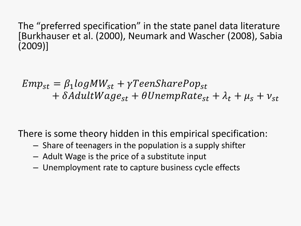
The “preferred specification” in the state panel data literature [Burkhauser et al. (2000), Neumark and Wascher (2008), Sabia (2009)] 𝐸𝑚𝑝𝑠𝑡 = 𝛽1𝑙𝑜𝑔𝑀𝑊𝑠𝑡 + 𝛾𝑇𝑒𝑒𝑛𝑆ℎ𝑎𝑟𝑒𝑃𝑜𝑝𝑠𝑡

+ 𝛿𝐴𝑑𝑢𝑙𝑡𝑊𝑎𝑔𝑒𝑠𝑡 + 𝜃𝑈𝑛𝑒𝑚𝑝𝑅𝑎𝑡𝑒𝑠𝑡 + 𝜆𝑡 + 𝜇𝑠 + 𝜈𝑠𝑡

There is some theory hidden in this empirical specification: – Share of teenagers in the population is a supply shifter – Adult Wage is the price of a substitute input – Unemployment rate to capture business cycle effects

Employment

Wage

D

S

W*

E*

Employment

Wage

D

S

Wmin

E* Emin

ΔEmp

𝐸𝑚𝑝𝑠𝑡 = 𝛽1𝑙𝑜𝑔𝑀𝑊𝑠𝑡 + 𝛾𝑇𝑒𝑒𝑛𝑆ℎ𝑎𝑟𝑒𝑃𝑜𝑝𝑠𝑡 + 𝛿𝐴𝑑𝑢𝑙𝑡𝑊𝑎𝑔𝑒𝑠𝑡

+ 𝜃𝑈𝑛𝑒𝑚𝑝𝑅𝑎𝑡𝑒𝑠𝑡 + 𝜆𝑡 + 𝜇𝑠 + 𝜈𝑠𝑡

𝛽1 ≈Δ𝐸𝑚𝑝

Δ𝑙𝑜𝑔𝑀𝑊

• Let’s count the number of employed workers in any period t:

• 𝐸𝑚𝑝𝑡 = 𝐸𝑚𝑝𝑡−1 + 𝐻𝑖𝑟𝑒𝑠𝑡 − 𝑆𝑒𝑝𝑎𝑟𝑎𝑡𝑖𝑜𝑛𝑠𝑡

=> ∆𝐸𝑚𝑝𝑡= 𝐻𝑖𝑟𝑒𝑠𝑡 − 𝑆𝑒𝑝𝑎𝑟𝑎𝑡𝑖𝑜𝑛𝑠𝑡

• Any effect on employment will be directly through the effects on hiring

and separations

• Key insight: Labor market policies (including minimum wages) can have drastic effects on hiring and separation rates, but result in a small net change in employment if those effects are similar.

The insight suggests that even without negative effects on employment, it is still important to understand how these policies affect workers’ ability to flow in and out of jobs.

– Turnover and market frictions

– Fluidity of labor markets in generating efficient matches

– Effects on the duration of unemployment

Similarly, beneath the surface, jobs can be reallocated across firms with no net change in aggregate employment

=> Focusing on employment misses a lot of action with regard to labor market dynamics

Residual Plot (CA) after removing state- and period-specific unobserved heterogeneity

Residual Plot (IL) after removing state- and period-specific unobserved heterogeneity

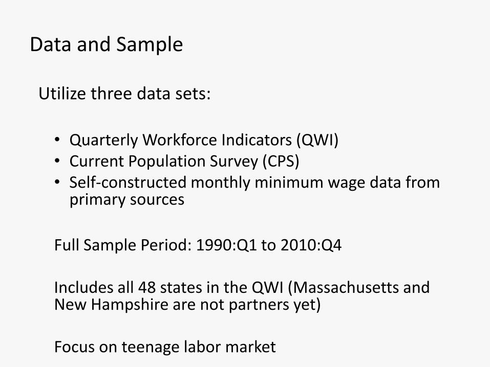
Data and Sample

Utilize three data sets:

• Quarterly Workforce Indicators (QWI) • Current Population Survey (CPS) • Self-constructed monthly minimum wage data from

primary sources

Full Sample Period: 1990:Q1 to 2010:Q4 Includes all 48 states in the QWI (Massachusetts and New Hampshire are not partners yet) Focus on teenage labor market

Quarterly Workforce Indicators (QWI) – Data product of the U.S. Census Bureau’s Longitudinal Employer

Household Dynamics program – Employer-employee matched data constructed from state

Unemployment Insurance (UI) records • UI records identifies the EIN of the employer, it’s industry code, and an

address, the SSN of worker and the worker’s taxable earnings • These data are then merged with data from the Social Security

Administration obtain other characteristics: age, sex and gender of the worker

– After processing, the data are aggregated to more coarse cells

for public use (State/Industry/Age group/Sex for example) that make up the QWI

– The individual micro data can also be merged with other data such as IRS tax records, the Current Population Survey, Survey of Income and Program Participation, criminal justice records, Annual Survey of Manufacturers, the Economic Census surveys.

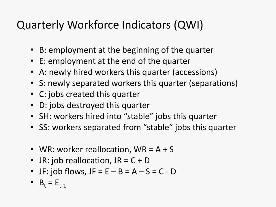
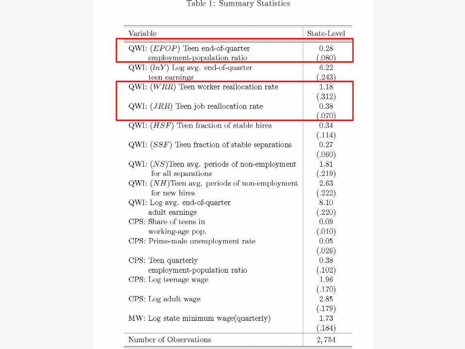
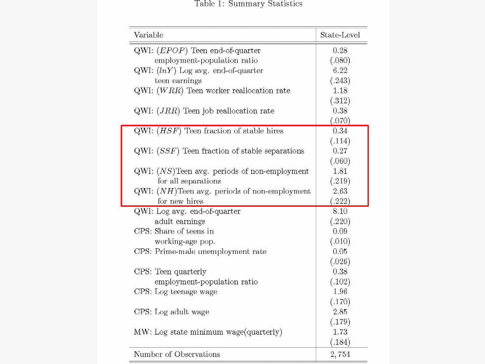
Quarterly Workforce Indicators (QWI) • B: employment at the beginning of the quarter • E: employment at the end of the quarter • A: newly hired workers this quarter (accessions) • S: newly separated workers this quarter (separations) • C: jobs created this quarter • D: jobs destroyed this quarter • SH: workers hired into “stable” jobs this quarter • SS: workers separated from “stable” jobs this quarter

• WR: worker reallocation, WR = A + S • JR: job reallocation, JR = C + D • JF: job flows, JF = E – B = A – S = C - D • Bt = Et-1

Minimum Wage Data

• Constructed from Bureau of Labor Statistics data, Monthly Labor Review, and states Department of Labor

• With quarterly data, it is important to get the timing right. We identify the month each minimum wage change occurs and can therefore attach the policy to the data in the proper time from.

• This is highly relevant: 290 total minimum wage changes 1990-2010 (≈ 6 per state) 43 percent occur in 1st quarter 4 percent occur in 2nd quarter 34 percent occur in 3rd quarter 19 percent occur in 4th quarter

Current Population Survey

• We use the CPS to estimate the state-level teen population and create control variables consistent with previous work – Teen population 16-19 (for employment/pop ratio) – Teen share of the population aged 16-65 – Wage rate of adults aged 25-54 – Male unemployment rate aged 25-54

• We also need the teen wage rate to determine the whether the minimum wage is binding (QWI only provides earnings)

Does the Minimum Wage Bind?

First order issue to the problem

Especially important for this work because you will see that higher minimum wages have no effect on teen earnings (=w*Hours)

– We will show that it does bind and shifts the lower half of the

teen wage distribution to the right.

– This, combined with no effect on earnings, suggests that there is an hours tradeoff on the intensive margin rather a worker reduction on the extensive margin.

– We simply note it here.

Table 2: MW Effects on the Teen Wage Distribution

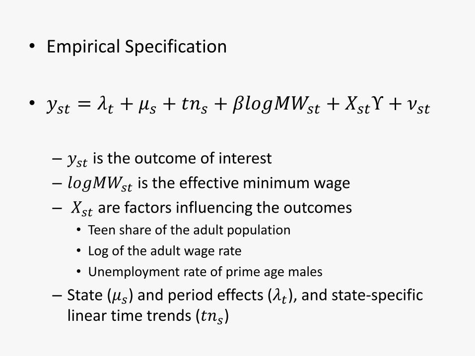
• Empirical Specification

• 𝑦𝑠𝑡 = 𝜆𝑡 + 𝜇𝑠 + 𝑡𝑛𝑠 + 𝛽𝑙𝑜𝑔𝑀𝑊𝑠𝑡 + 𝑋𝑠𝑡Υ + 𝜈𝑠𝑡

– 𝑦𝑠𝑡 is the outcome of interest

– 𝑙𝑜𝑔𝑀𝑊𝑠𝑡 is the effective minimum wage

– 𝑋𝑠𝑡 are factors influencing the outcomes

• Teen share of the adult population

• Log of the adult wage rate

• Unemployment rate of prime age males

– State (𝜇𝑠) and period effects (𝜆𝑡), and state-specific linear time trends (𝑡𝑛𝑠)

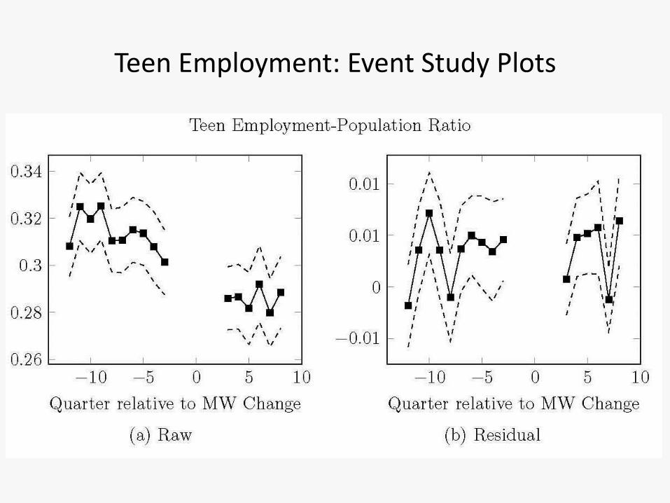
Teen Employment: Event Study Plots

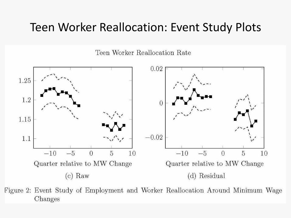
Teen Worker Reallocation: Event Study Plots

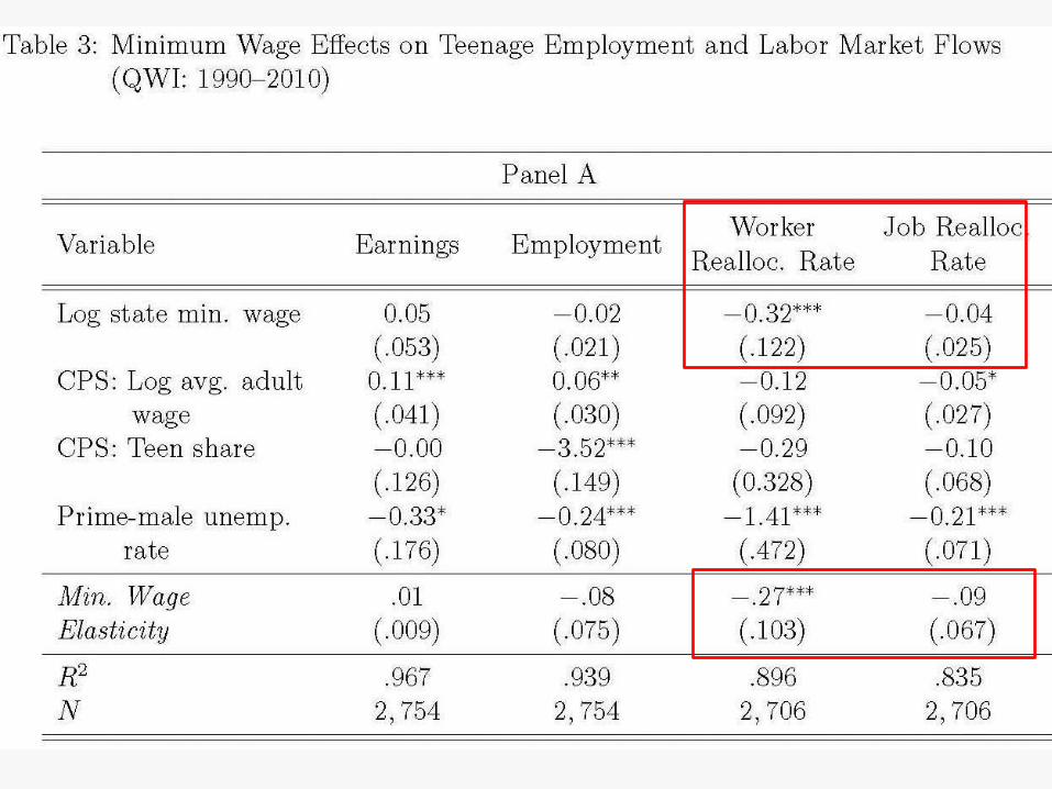
1) No effect on employment or earnings (possible hours

tradeoff)

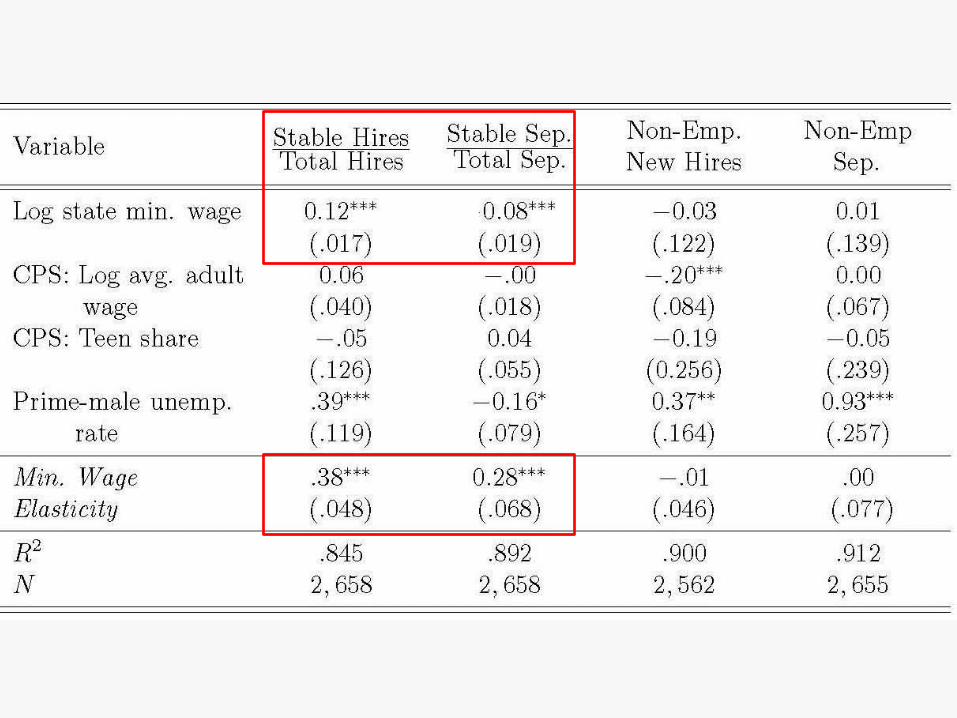
2) Large reductions in the rate at which workers flow into and out of jobs, but jobs are not reallocated across employers

3) Increases in jobs stability (tenure of employed workers) 2) and 3) imply an increase in the duration of unemployment

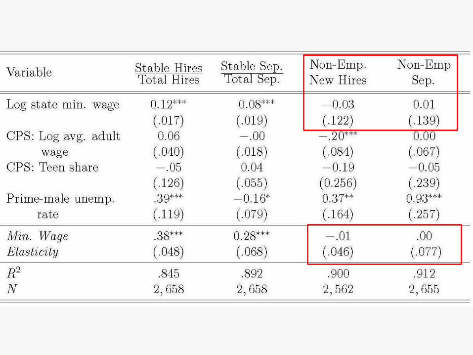
4) No change in periods of non-employment not a measure of unemployment but also coarsely measured in terms of quarters

Robustness Checks Concern that entry dates for states into the QWI may generate a selection problem

• Restrict sample to post-2000 period where entry is the same and panel is balanced

Minimum wage effects may occur with some lag (Baker et al. 1999; Burkhauser et al. 2000)

Unobserved state-specific seasonality

Take advantage of county-level variation in labor market variables in the QWI

The Interaction Between Turnover and Employment

Turnover plays an important role in labor markets as a basic barometer of labor market health or as a reflection of labor market frictions

• Lazear and Spletzer (2012): (1) low turnover markets can be problematic because they prevent more productive matches. (2) reductions in turnover can be efficiency-enhancing if turnover is higher than necessary to allocate resources

Minimum wage effects on employment may vary depending on the level of turnover in the market

• Take advantage of industry-level detail in QWI to identify low turnover and high turnover labor markets within states.

Disemployment Effects Vary by Market Turnover

Two Possible Models to Contrast the Pattern in the Data Wage Posting Model

• High rates of turnover are reflected by high rates of poaching by competing firms

• In this model, high turnover markets are highly competitive markets (low friction markets)

• Therefore, stronger disemployment effects are predicted in markets with higher levels of turnover

Turnover as a Cost Channel for Firms

• Simplified version of Manning (2006) but we make the role of turnover explicit

• Efficiency wage model where firms face adjustment costs (recruiting and training costs) and a mobile workforce

• Turnover is costly, but the firm can reduce turnover by offering higher wages

• Therefore, higher minimum wages affect both unit labor costs and recruiting costs. Which effect dominates determines the resulting effect on employment.

Turnover as a Cost Channel for Firms

Firm of size N faces chooses a wage rate to max profits

• Labor is the only input

• Separation rate: s(w)

• Efficiency wages: s’(w) < 0

• H=s(w)N number or workers must be replaced each period

• A(H) is cost of recruiting H workers, A’(H) > 0, A’’(H) > 0

• The wage rate, w, is unit cost of labor

To maximize profits the firm offers a wage rate that minimizes labor costs, conditional on employing N workers.

Turnover as a Cost Channel for Firms

Firm’s Problem:

𝑚𝑖𝑛𝑤 𝑤𝑁 + 𝐴 𝐻

𝑠. 𝑡. 𝐻 = 𝑠 𝑤 𝑁; 𝑤 ≥ 𝑤𝑚𝑖𝑛

Let w* be the optimal wage satisfying this problem.

At w*, we want to know how minimum wages affect the marginal cost of labor (and hence employment).

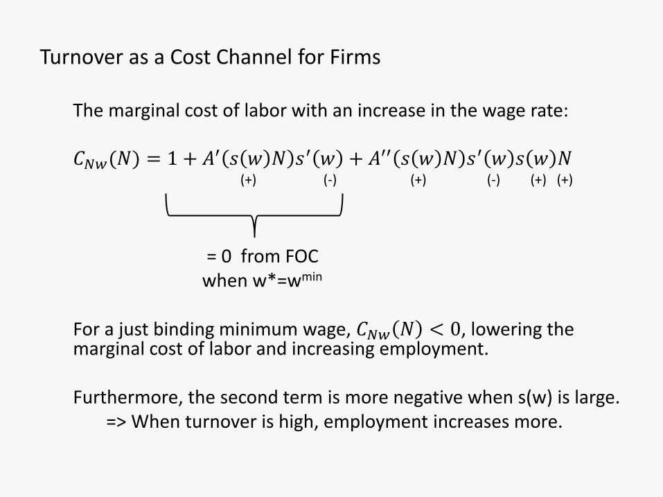
Turnover as a Cost Channel for Firms The marginal cost of labor with an increase in the wage rate:

𝐶𝑁𝑤(𝑁) = 1 + 𝐴′ 𝑠 𝑤 𝑁 𝑠′ 𝑤 + 𝐴′′ 𝑠 𝑤 𝑁 𝑠′ 𝑤 𝑠 𝑤 𝑁

(+) (-) (+) (-) (+) (+)

= 0 from FOC when w*=wmin

For a just binding minimum wage, 𝐶𝑁𝑤 𝑁 < 0, lowering the marginal cost of labor and increasing employment. Furthermore, the second term is more negative when s(w) is large. => When turnover is high, employment increases more.

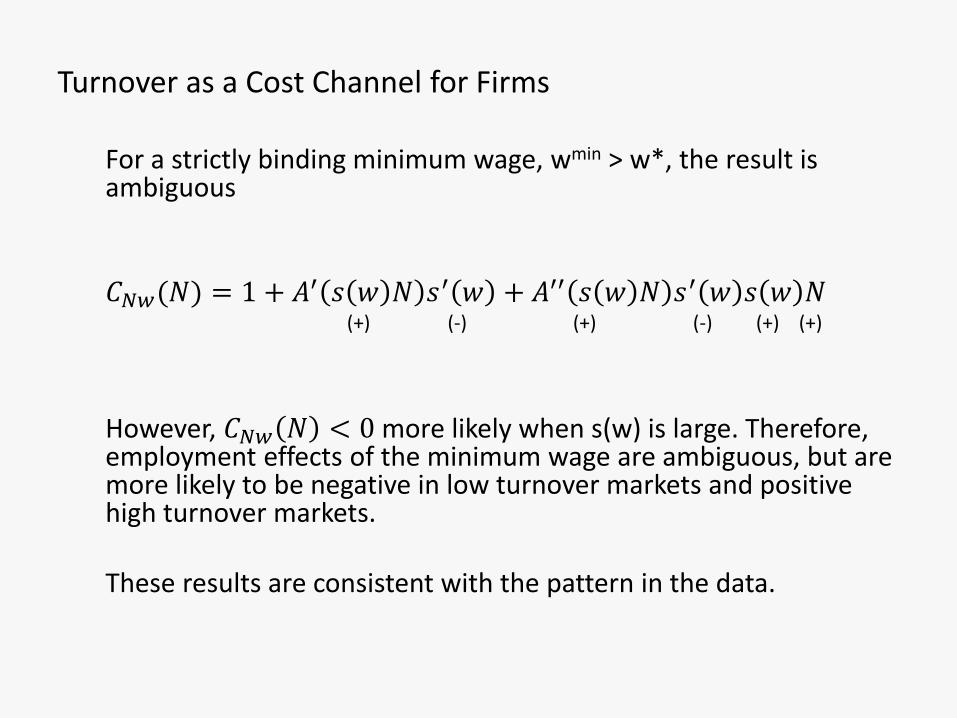
Turnover as a Cost Channel for Firms For a strictly binding minimum wage, wmin > w*, the result is ambiguous

𝐶𝑁𝑤(𝑁) = 1 + 𝐴′ 𝑠 𝑤 𝑁 𝑠′ 𝑤 + 𝐴′′ 𝑠 𝑤 𝑁 𝑠′ 𝑤 𝑠 𝑤 𝑁 (+) (-) (+) (-) (+) (+)

However, 𝐶𝑁𝑤 𝑁 < 0 more likely when s(w) is large. Therefore, employment effects of the minimum wage are ambiguous, but are more likely to be negative in low turnover markets and positive high turnover markets. These results are consistent with the pattern in the data.

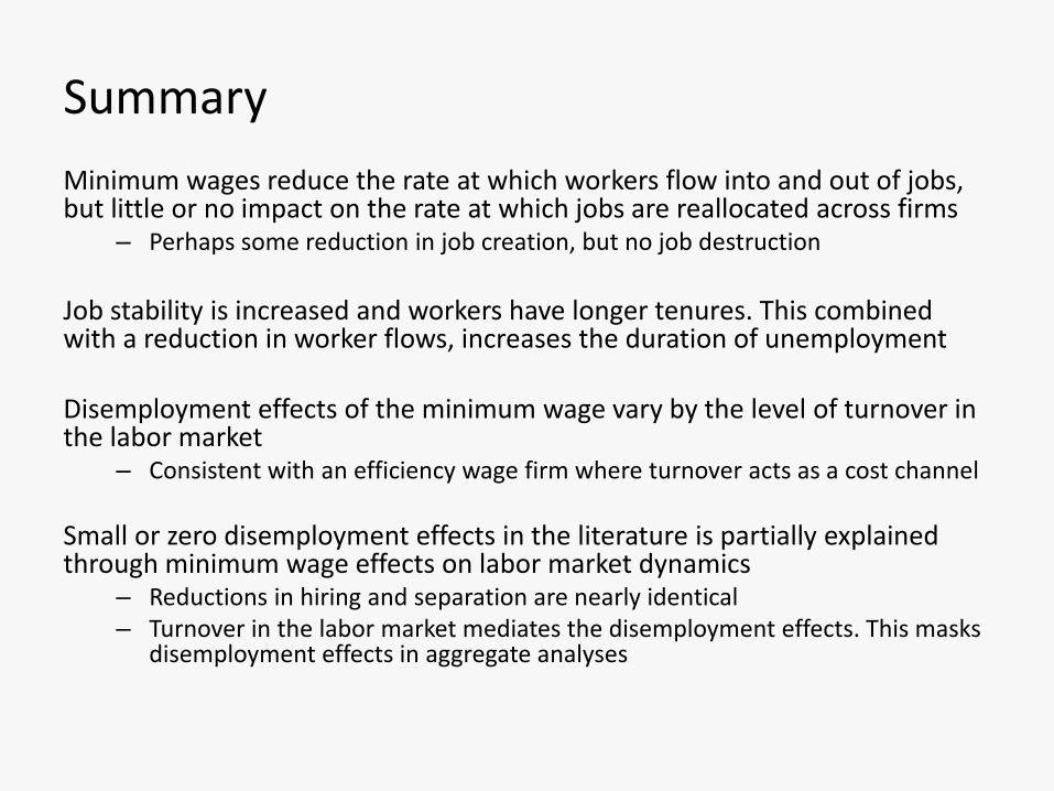
Summary

Minimum wages reduce the rate at which workers flow into and out of jobs, but little or no impact on the rate at which jobs are reallocated across firms

– Perhaps some reduction in job creation, but no job destruction

Job stability is increased and workers have longer tenures. This combined with a reduction in worker flows, increases the duration of unemployment

Disemployment effects of the minimum wage vary by the level of turnover in the labor market

– Consistent with an efficiency wage firm where turnover acts as a cost channel

Small or zero disemployment effects in the literature is partially explained through minimum wage effects on labor market dynamics

– Reductions in hiring and separation are nearly identical – Turnover in the labor market mediates the disemployment effects. This masks

disemployment effects in aggregate analyses

Where to Go From Here

• Do the analysis at the firm level (restricted data) – job reallocation across firms and industries is masked in aggregate data. – Restricted data have detail on firm size, “types” or workers employed, and

more specific identification about the labor market the firm participates iin – MW data is ported on the confidential server and ready

• Investigate direct effect on duration of unemployment and hours

• Labor-Labor trade off

– Newly released versions of QWI data disaggregates labor market data by race and education

• Empirical specification based on static theory: Introduce dynamics

explicitly and exploit the high frequency data (monthly/quarterly). – MW policy announced well into the future. Firms forward looking? – Labor market variables explicitly linked through identities.

• => Intertemporal MW effects and structural VAR estimation?