GEOSPATIAL THINKING OF UNDERGRADUATE STUDENTS IN …

GEOSPATIAL THINKING OF UNDERGRADUATE STUDENTS IN PUBLIC

UNIVERITIES IN THE UNITED STATES

by

Kanika Verma, M.A., B.Ed., B.A.

A dissertation submitted to the Graduate Council of Texas State University in partial fulfillment

of the requirements for the degree of Doctor of Philosophy

with a Major in Geographic Education May 2014

Committee Members:

Lawrence E. Estaville, Chair

Brock Brown

T. Edwin Chow

Niem T. Huynh

COPYRIGHT

by

Kanika Verma

2014

FAIR USE AND AUTHOR’S PERMISSION STATEMENT

Fair Use

This work is protected by the Copyright Laws of the United States (Public Law 94-553, sections 107). Consistent with fair use as defined in the Copyright laws, brief quotations from this material are allowed with proper acknowledgement. Use of this material for financial gain without the author’s express written permission is not allowed.

Duplication Permission

As the copyright holder of this work I, Kanika Verma, authorize duplication of this work, in whole or in part, for educational or scholarly purposes only.

DEDICATION

To my parents, Vijay Verma and Anupam Verma, my husband, Nikhil Chawla,

my son, Aryaveer Chawla, and my siblings, Tanika Verma and Jaideep Verma.

v

ACKNOWLEDGEMENTS

I owe my most sincere gratitude to my advisor, Dr. Lawrence Estaville, for his

expert guidance, empathetic mentorship, unconditional support, and confidence in my

abilities. His tireless dedication to my academic and professional career has given me

immense strength during my doctoral journey. This dissertation would not have been

accomplished without his patience and continuous encouragement.

I wholeheartedly thank the members of my dissertation committee for their

guidance and support in the completion of my dissertation and in other research projects

during my entire doctoral career. Dr. Brock Brown’s vast knowledge of geography and

his passion for the advancement of geography education expanded my academic

experiences. Dr. Edwin Chow’s great knowledge and experience in statistical methods

served as an invaluable asset to my dissertation. Dr. Niem Huynh’s expertise and

leadership in the field of geospatial thinking provided significant insight to my

dissertation.

I deeply thank my father, Vijay, my mother, Anupam, my husband and best

friend, Nikhil, my brother-in-law, Rajan, and my sister-in-law, Manav, for providing me

with the means, encouragement, and strength to complete my doctoral studies. I greatly

owe my parents and husband most of what I am today. I genuinely thank Nikhil for his

unwavering love, endless patience, constant belief in me, and sincere encouragement to

explore the unknown. I thank my siblings, Tanika and Jaideep, for being my emotional

and moral strengths, for cheering me up in difficult times, and for assisting me in

vi

realizing my own potentials. Also, I would like to thank my precious son, Aryaveer,

whose smiles and innocence have filled my life with joy. His very presence gave me the

ultimate push to finish my work each day.

I would also like to thank the faculty members, my friends, and colleagues in the

Department of Geography and other departments at Texas State University. Special

thanks go to Phillicia Phillips for her expert help with the maps used in this dissertation,

Nikhil, for providing invaluable help with data handling, and Graciela Sandoval, for

editing the images used in the survey. I also owe my sincere acknowledgement to

geography faculty across the country who encouraged their students to participate in the

national online survey, students who volunteered their time to complete the Geospatial

Thinking Survey, and to instructors who participated in the phone interviews.

I also want to extend my gratitude to the Graduate College, Associated Student

Government, and the Department of Geography at Texas State University, and to the

Golden Key International Honour Society for awarding generous scholarships to

complete my doctoral studies.

vii

TABLE OF CONTENTS

Page

ACKNOWLEDGEMENTS .................................................................................................v

LIST OF TABLES ...............................................................................................................x

LIST OF FIGURES ...........................................................................................................xv

ABSTRACT ..................................................................................................................... xvi

CHAPTER

I. INTRODUCTION .......................................................................................1

Significance of the Study ...........................................................................10 Problem Statement .....................................................................................12

II. LITERATURE REVIEW ..........................................................................14

Frameworks for Understanding Spatial and Geospatial Thinking .............15 Group Differences in Spatial and Geospatial Thinking .............................23 Effects of Interventions on Spatial and Geospatial Thinking ....................35 Linking the Literature Review and Problem Statement .............................39 Theoretical Framework ..............................................................................40

III. METHOD ..................................................................................................47

Research Hypotheses and Questions .........................................................47 Quantitative Research Question .....................................................47 Quantitative Research Hypotheses ................................................47 Qualitative Research Questions .....................................................48 Qualitative Research Hypothesis ...................................................49

Data Collection ..........................................................................................49 Characteristics of the Test Instrument .......................................................51

Reliability and Validity ..................................................................53 Domains of Geospatial Thinking ...............................................................55 Quantitative Analyses ................................................................................55

Variables ........................................................................................55

viii

Student Performance Measured by GTS Score: Geospatial Thinking Index (GTI) ....................................................................56 Group Differences on GTS Score Means ......................................56 Geospatial Thinking Score Prediction ...........................................57 Student Performance on Individual Questions of the GTS ............57 Group Differences on Individual Questions of the GTS ...............58

Qualitative Analyses ..................................................................................58 Mixed-method Analysis .............................................................................59

IV. QUANTITATIVE ANALYSES AND FINDINGS ...................................60

Domains of Geospatial Thinking ...............................................................60 Student Performance Measured by GTS score: Geospatial Thinking Index (GTI) ..................................................63 Group Differences on GTS Score Means ..................................................65 Geospatial Thinking Score Prediction: Regression Model ........................81 Geospatial Thinking Score Prediction: Data Mining Model .....................89 Student Performance on Individual Questions of the GTS ........................94 Group Differences on Individual Questions of the GTS ...........................98 Visualization of Responses for Individual GTS Questions .....................121 Quantitative Study Limitations and Discussion of Error .........................127 Summary of Major Quantitative Findings ...............................................128

V. QUALITATIVE ANALYSES AND FINDINGS ...................................131

Qualitative Data .......................................................................................131 Qualitative Analyses ................................................................................133

Geospatial Concepts .....................................................................133 Tools of Representation ...............................................................134 Processes of Reasoning ................................................................134 Other Thoughts ............................................................................135

Mixed-method Analysis ...........................................................................136 Qualitative Study Limitations and Discussion of Error ...........................138 Summary of Major Qualitative Findings .................................................138

VI. CONCLUSIONS AND FUTURE RESEARCH .....................................140

Conclusions ..............................................................................................140 Quantitative Research Question ...................................................140 Quantitative Research Hypotheses ..............................................140 Qualitative Research Questions ...................................................141

ix

Qualitative Research Hypothesis .................................................141 Discussion of Quantitative Findings ........................................................141 Discussion of Qualitative Findings ..........................................................147 Linking Findings to Theory .....................................................................147 Future Research .......................................................................................148

APPENDIX SECTION ....................................................................................................150

WORKS CITED ..............................................................................................................160

x

LIST OF TABLES

Table Page

2.1 Classification of Spatial Thinking Concepts, Components, and Domains ............19

2.2 Classification of Spatial Scales ..............................................................................22

2.3 Selected Research Works about Group Differences in Spatial and Geospatial Thinking in Geography and Other Disciplines: 1970-2013 .......................34

3.1 Distribution and Number of Undergraduate Students Who Completed the Geospatial Thinking Survey (GTS) by Census Division (Number of Universities) ...............................................................................................51

3.2 Geospatial Thinking Domains in the Geospatial Thinking Survey (GTS): Based on Golledge (1995, 2002); Gersmehl and Gersmehl (2006); Jo and Bednarz (2009); and Lee and Bednarz (2012) ...........................................52

4.1 Results of Principal Component Analysis (PCA) for the GTS ..............................61

4.2 GTS Scores and Student Frequencies ....................................................................63

4.3 Geospatial Thinking Index .....................................................................................65

4.4 GTS Score Means for Sex ......................................................................................66

4.5 GTS Score Means for Age Categories ...................................................................66

4.6 Post-hoc Comparisons (Games-Howell) of GTS Score by Age Categories (p Value in Parentheses) .................................................................................67

4.7 GTS Score Means for Ethnic Groups ....................................................................67

4.8 Post-hoc Comparisons (Games-Howell) of GTS Score by Ethnic Groups (p Value in Parentheses) ...........................................................................................68

4.9 GTS Score Means for Parents’ Annual Income Categories ...................................68

4.10 Post-hoc Comparisons (Games-Howell) of GTS Score by Parents’ Annual Income Categories (p Value in Parentheses) ..........................................................69

4.11 GTS Score Means for Parents’ Education Categories ...........................................69

xi

4.12 Post-hoc Comparisons (Games-Howell) of GTS Score by Parents’ Education Categories (p Value in Parentheses) ..........................................................70

4.13 GTS Score Means for Academic Classifications ...................................................70

4.14 Post-hoc Comparisons (Games-Howell) of GTS Score by Academic Classifications (p Value in Parentheses) ....................................................71

4.15 GTS Score Means for Academic Majors ...............................................................72

4.16 Significant Post-hoc Comparisons (Games-Howell) of GTS Score by Academic Majors (p Value in Parentheses) ................................................................73

4.17 GTS Score Means for Number of High School Geography Courses ....................74

4.18 Post-hoc Comparisons (Games-Howell) of GTS Score by Number of High School Geography Courses (p Value in Parentheses) ............................................75

4.19 GTS Score Means for the Number of College Geography Courses ......................75

4.20 Post-hoc Comparisons (Games-Howell) of GTS Score by Number of College Geography Courses (p Value in Parentheses) ............................................76

4.21 GTS Score Means for Geography Department Degree Levels ..............................76

4.22 GTS Score Means for Urban/Suburban/Rural Patterns .........................................77

4.23 Post-hoc Comparisons (Games-Howell) of GTS Score by Urban/Suburban/Rural Patterns (p Value in Parentheses) ..............................................................78

4.24 GTS Score Means for Census Divisions ................................................................78

4.25 Post-hoc Comparisons (Games-Howell) of GTS Score by Census Divisions (p Value in Parentheses) .................................................................................79

4.26 Summary of Highest and Lowest GTS Mean Scores for Significant Variables ....81

4.27 Results of CATPCA of the Independent Variables ...............................................83

4.28 Multiple Regression Model for Predicting Geospatial Thinking Scores ...............84

4.29 Coefficients of the Multiple Regression Model for Predicting Geospatial Thinking Scores .........................................................................................................84

xii

4.30 Multiple Regression Model for Predicting Academic Component Values ...........86

4.31 Coefficients of the Multiple Regression Model for Predicting Academic Component Values .....................................................................................86

4.32 Multiple Regression Model for Predicting Socioeconomic Component Values ...87

4.33 Coefficients of the Multiple Regression Model for Predicting Socioeconomic Component Values .....................................................................................88

4.34 Cubist First-Run Model to Predict Students’ Geospatial Thinking Score (GT Score) .........................................................................................................91

4.35 Cubist Second-Run Model to Predict Students’ Geospatial Thinking Score (GT Score) .........................................................................................................93

4.36 Difficulty Level of GTS Questions Based on Students’ Responses (From Less Difficult to More Difficult) ........................................................................95

4.37 Association of Q1 (Geospatial Pattern and Transition) with Sex, Age, Ethnicity, Academic Classification, College Geography, and Urban/Suburban/Rural Patterns .......................................................................................................99

4.38 Internal Comparisons for Association of Q1 (Geospatial Pattern and Transition) with Ethnicity, Academic Classification, College Geography, and Urban/Suburban/Rural Patterns ...............................................................100

4.39 Association of Q2 (Direction and Orientation) with Sex, Age, Ethnicity, Academic Classification, College Geography, and Urban/Suburban/Rural Patterns .....................................................................................................101

4.40 Internal Comparisons for Association of Q2 (Direction and Orientation) with Ethnicity, and Urban/Suburban/Rural Patterns ........................................102

4.41 Association of Q3 (Geospatial Profile and Transition) with Sex, Age, Ethnicity, Academic Classification, College Geography, and Urban/Suburban/Rural Patterns .....................................................................................................103

4.42 Internal Comparisons for Association of Q3 (Geospatial Profile and Transition) with Sex, Age, Ethnicity, Academic Classification, College Geography, and Urban/ Suburban/Rural Patterns .......................................................104

xiii

4.43 Association of Q4 (Geospatial Association and Transition) with Sex, Age, Ethnicity, Academic Classification, College Geography, and Urban/Suburban/Rural Patterns ...............................................................106

4.44 Internal Comparisons for Association of Q4 (Geospatial Association and Transition) with Age, and Academic Classification ................................107

4.45 Association of Q5 (Geospatial Association) with Sex, Age, Ethnicity, Academic Classification, College Geography,

and Urban/Suburban/Rural Patterns ........................................................108

4.46 Internal Comparisons for Association of Q5 (Geospatial Association) with Sex, Age, Ethnicity, Academic Classification, College Geography, and Urban/Suburban/Rural Patterns ...............................................................109

4.47 Association of Q6 (Geospatial Shapes) with Sex, Age, Ethnicity, Academic Classification, College Geography,


4.48 Internal Comparisons for Association of Q6 (Geospatial Shapes) with Sex, Age, Ethnicity, Academic Classification, College Geography, and Urban/Suburban/Rural Patterns ...............................................................111



4.50 Internal Comparisons for Association of Q7 (Geospatial Shapes) with Age, Ethnicity, Academic Classification, and College Geography ..................113



4.52 Internal Comparisons for Association of Q8 (Geospatial Shapes) with Sex, Age, Ethnicity, Academic Classification, College Geography, and Urban/Suburban/Rural Patterns ...............................................................115



xiv

4.54 Association of Q10 (Geospatial Overlay) with Sex, Age, Ethnicity, Academic Classification, College Geography,


4.55 Internal Comparisons for Association of Q10 (Geospatial Overlay) with Sex, Age, Ethnicity, Academic Classification, and College Geography ..................119

4.56 Summary of Relationship of Geospatial Thinking Domains with Significant Variables ..................................................................................................120

5.1 Background of Faculty Interviewed (percentages to total) ..................................132

5.2 Comparison of Quantitative Data (GTS Scores for Domains/Questions) and Qualitative Data (Instructor Perceptions of Student Geospatial Thinking) ..................................................................................................137

xv

LIST OF FIGURES

Figure Page

2.1 Application of Vygotsky’s (1978) Sociocultural Theory of Psychological Process (STPP) to geospatial thinking and its learning by students .......................46

3.1 Location of sample universities in the U.S. census divisions for student data (n = 61) ..................................................................................50

4.1 Histogram of student performance on the GTS .....................................................64

4.2 Student performance on individual GTS questions ...............................................94

4.3 Student performance on GTS questions based on sex .........................................122

4.4 Student performance on GTS questions based on age .........................................123

4.5 Student performance on GTS questions based on ethnicity ................................124

4.6 Student performance on GTS questions based on academic classification .........125

4.7 Student performance on GTS questions based on number of college geography courses taken ............................................................................................126

4.8 Student performance on GTS questions based on urban/suburban/rural locations .................................................................127

5.1 Location of sample universities in the U.S. census divisions for faculty interview data (n = 27) .............................................................................................132

xvi

ABSTRACT

Geospatial thinking and learning are essential components of geography

education. The National Research Council’s 2006 report, Learning to Think Spatially,

emphasized that people vary with respect to performance on spatial tasks. Geospatial

thinking is a subset of spatial thinking in general. Geospatial thinking is using Earth

space at different scales to structure problems, find answers, and express solutions using

geospatial concepts, tools of representation, and reasoning processes. Scholars in

geography and other disciplines have studied group differences in spatial and geospatial

thinking focusing on sex, age, and school grade-level. This dissertation utilized

additional demographic variables, such as ethnicity and socioeconomic status, academic

variables, such as academic majors and geography academic experience, and geographic

locational variables, such as census divisions and urban/suburban/rural locations, to

explore group differences in geospatial thinking.

The national study in this dissertation utilized Geospatial Thinking Survey (GTS),

based on Spatial Thinking Ability Test (STAT) (Lee and Bednarz 2012), to assess group

variances in geospatial thinking abilities of undergraduate students (n = 1479) in 61

public universities in 32 states across nine census divisions of the United States. This

mixed-method study investigated whether some groups of students, such as ethnic groups

or academic major groups, outperform others in overall geospatial thinking and in

separate geospatial thinking domains, such as geospatial association and geospatial

overlay, and matched students’ performance on the GTS with instructors’ perceptions of

xvii

students’ geospatial thinking skills. This dissertation also undertook statistical and data-

mining modeling to predict the geospatial thinking score of undergraduate students based

on demographic and academic characteristics.

The quantitative findings of this research showed that ethnicity, along with

socioeconomic status, and geography courses are the most important variables in

understanding, influencing, and predicting undergraduate students’ geospatial thinking in

the United States. Geography educators must tailor classroom instruction and curricula to

help improve geospatial thinking of underperforming ethnic groups, especially blacks and

Hispanics. The qualitative findings of this study revealed that college geography

educators do not have a clear perception of their students’ geospatial thinking, because

instructors are not fully utilizing geospatial tools of representation, such as maps, to

improve the understanding of geospatial concepts in their students.

1

CHAPTER I

INTRODUCTION

A groundbreaking publication by the National Research Council (NRC), Learning

to Think Spatially (NRC 2006), offered a new approach to spatial thinking. The report

argued that spatial thinking is universal and malleable. The basic building block for

spatial thinking is space, and the operations that humans can perform in space form its

foundation. Within his space-time theory of relativity, Albert Einstein conceptualized

space as the distance or expanse among objects—relative space (Isaacson 2007).

Spatial thinking—a constructive combination of concepts of space, tools of

representation, and processes of reasoning—uses space to structure problems, find

answers, and express solutions (NRC 2006). Spatial thinking is a cognitive ability to

visualize and interpret location, position, distance, direction, relationships, movement,

and change over space, in different situations and at different scales (Sinton et al. 2013).

“Spatial thinking means different things at different scales, and within different academic

disciplines” (DiBiase 2013). Geospatial thinking, focusing on the geography of human

life spaces (spatial thinking at the level of Earth), is a subset of spatial thinking in general

(Golledge, Marsh, and Battersby 2008b). Thus, geospatial thinking is using Earth space

or geographic space at different scales to frame problems, identify answers, and provide

solutions using geospatial concepts, representation tools, and reasoning processes. Spatial

thinking is powerful and pervasive in academic disciplines, the workplace, and everyday

problem-solving situations. The 2006 NRC report also highlighted that spatial thinking

can and should be taught at all levels in the educational system. Skills and strategies for

2

using and applying spatial thinking to solve academic and everyday problems can be

learned. “Spatial thinking is a skill or a collection of skills that are all learnable, and can

be taught” (Huynh and Sharpe 2013, 4). The NRC report, thus, strongly recommended

that a systematic research program into the nature, characteristics, and operations of

spatial thinking should be undertaken. A national commitment should undergird the

systematic educational efforts necessary to meet the goal of spatial literacy (NRC 2006).

Spatial thinking is an important part of any curriculum. Liben (2006) emphasized the

importance and pervasiveness of spatial thinking and its value in a wide range of

disciplines, concepts, tasks, and settings. Spatial thinking plays fundamental roles in

scientific and educational research (Newcombe 2010). Spatial thinking is critical in

theory-building (e.g., central place theory) and scientific visualization (e.g., sea floor

mapping) (NRC 2006).

The inherent link among the elements of space, representation, and reasoning

provides power, versatility, and applicability to the process of spatial thinking. Myriad

ways exist to approach spatial thinking and to think spatially. The ability to use and apply

spatial concepts, representations, and reasoning intelligently and critically is becoming

more crucial when participating in academic, workplace, and everyday settings of the

modern society. Various spatial thinking modes are connected to brain locations that

undertake verbal and mathematical reasoning (Gersmehl and Gersmehl 2007b). Spatial

training has been found to improve educational outcomes, such as helping college

students complete engineering degrees (Newcombe 2010). Spatial thinking training in

education will increase student participation in mathematics, science, and engineering

careers (Uttal et al. 2013). The information technology sector is continuously demanding

3

skilled workers with spatial skills (NRC 2006). Neurosurgeons, for example, draw on

magnetic resonance imaging (MRI) to visualize specific brain areas that may determine

the outcomes of surgical procedures (Newcombe 2010). The U.S. Department of Labor

has required geospatial talents in their career opportunities (Baker 2012).

People think spatially in many everyday situations: when rearranging clothes in a

luggage bag, assembling a piece of furniture using a diagram, buying a new home,

placing dishes on a dinner table, or consulting a map for directions. “We understand

things by looking at their spatial patterns” (Sinton et al. 2013, 11). Geospatial knowledge

helps us to make sense of chaotic and diversified environments (Golledge 2002).

Geospatial thinking is important for significant everyday life exercises such as

remembering a specific map, route planning, following directions to a location,

calculating distances and directions, determining spatial patterns among different features

on land, visualizing 3-D topography from an alternative perspective, or choosing the best

location based on given geographical criteria. Geographic behavior in day-to-day human

actions is an essential part of geospatial thinking. Blaut (1991) describes geographic

behavior as macro-environmental behavior or place behavior, involving human

interaction with the environment or the place, observed in all cultures. “As spatial

thinking abilities become increasingly recognized as important for understanding

geography, math, science, engineering, and many aspects of everyday life, it is clear that

the understanding of these concepts, no matter how simple they seem, must no longer be

taken for granted” (Marsh, Golledge, and Battersby 2007, 711).

Despite its crucial role underpinning the National Standards for Science,

Mathematics, and Geography, spatial thinking is currently not systematically

4

incorporated into the educational curricula at the K-12 and post-secondary levels. “The

development of spatial thinking is not an explicit goal of any school curriculum as

literacy and numeracy are” (Sinton et al. 2013, 63). Spatial thinking must be recognized

as a fundamental part of the educational system and as a means of facilitating problem-

solving and better performance across the academic, professional, and day-to-day

activities. Our school systems emphasize reading, writing, math, and science (Sword

2001; Wai 2012; Uttal et al. 2013). Absence of explicit spatial thinking content in the

school curriculum will not recognize, support, and challenge the talents of students with

strong spatial thinking skills (Sword 2001; Sinton et al. 2013; Uttal et al. 2013). Wai

(2012) stressed that some school children are good at numbers and words, while others

are better at thinking spatially or visualizing shapes and figures in their minds. All great

inventors of the world were not necessarily good at writing essays or solving

mathematical equations, they rather imagined spatial models in their minds and made

important discoveries (Wai 2012). If school education continues to ignore and undermine

students with spatial intelligence, then society will marginalize exceptional spatial talents

that can design and build maps, geospatial models, art, buildings, bridges, mechanical

devices, engineered tools, electronic devices, smart toys and gadgets. The 2006 NRC

report identified its predominant goal as fostering “a generation of students (1) who have

the habit of mind of thinking spatially, (2) who can practice spatial thinking in an

informed way, and (3) who adopt a critical stance to spatial thinking” (NRC 2006, 3-4).

To find ways to facilitate students’ application of spatial thinking and to encourage

spatial literacy in students is thus imperative. However, the NRC report made it very

clear that spatial thinking is not an add-on to an already crowded school curricula, but

5

rather a missing link across curricula. “Integration and infusion of spatial thinking can

help to achieve existing curricular objectives. Spatial thinking is another level to enable

students to achieve a deeper and more insightful understanding of subjects across the

curriculum” (NRC 2006, 26). Hespanha, Goodchild, and Janelle (2009) observed that

explicit practice of spatial thinking in undergraduate social science courses is lacking.

The researchers discussed insights and strategies emerging from National Science

Foundation (NSF)-sponsored SPACE (Spatial Perspectives on Analysis for Curriculum

Enhancement) workshops on spatial thinking in undergraduate education. Sinton et al.

(2013) recognized the importance of spatial thinking both as a horizontal thread across

the curriculum (learning to understand and practice spatial thinking in all school subjects)

and a vertical thread up through the curriculum (from kindergarten through college).

The BRAIN Initiative (2013) is President Obama’s recent call to the science

community to undertake research in human brain functioning. BRAIN stands for Brain

Research through Advancing Innovative Neurotechnologies. One of the many goals of

this program is to understand how brain activity leads to perception, decision-making,

and ultimately action. The complex and dynamic nature of human brain calls for

uncovering truths and trends about how people think spatially and use spatial thinking

strategies in everyday life (Sinton et al. 2013). Gersmehl (2012) presented recent trends

in neuroscience research asserting that the human brain seems to be “hard-wired” for

spatial thinking, mathematics, and language. Gersmehl (2012) referred to Immanuel

Kant’s monumental work “Critique of Pure Reason” (1781) to rationalize that the brain is

predisposed to think in certain ways and postulated that people have three a priori ways

of organizing information from experience—temporally, spatially, and causally

6

(Gersmehl 2012). Gersmehl (2012) conceptualized that different regions of the brain

perform distinct spatial thinking skills, based on more than 3000 research studies. fMRI

(functional MRI) and other brain-scanning technologies clearly show that the typical

human brain has as many as 8-10 distinct areas that take part in thinking in, about, and

with space, such as comparing conditions in different places, grouping places into

regions, arranging places in sequences, and finding positions in spatial hierarchies

(Sinton et al. 2013). Thus, ignoring spatial and geospatial thinking education directly

implies neglecting one of the key ways with which human brain organizes knowledge.

Spatial thinking is an important life-skill that also improves overall academic

performance. Spatial thinking skills are an essential component of an array of skills that

are required for problem solving to assist durable learning (Gersmehl and Gersmehl

2006). Providing a more prominent place for spatial thinking skills in the curricula and

assessment programs of American schools (Gersmehl and Gersmehl 2006), starting in

kindergarten and first grade (Gersmehl and Gersmehl 2007a), is favorable for student

performance. Understanding spatial and geospatial thinking is, thus, an important part of

the BRAIN Initiative (2013). Spatial and geospatial thinking research will reveal new

agendas about human cognition that now can only be imagined (Sinton et al. 2013).

The Rediscovering Geography Committee (1997) recommended undertaking

research that improves the understanding of geographic literacy and learning.

“Geographical learning requires a geographical lens, an approach that is grounded in

spatial thinking” (Sinton et al. 2013, 13). Cutter, Golledge, and Graf (2002, 315)

structured ten questions important for the geographic community to address: the tenth

question was “what is the nature of spatial thinking, reasoning, and abilities?” They

7

declared that geographic knowledge is the product of spatial thinking and reasoning

requiring the ability to comprehend such concepts as scale changes, distance and

direction variations, and location identification. Spatial thinking concepts are most

closely associated with the discipline of geography and geographic knowledge (Tate,

Jarvis, and Moore 2005). The concepts, representations, and processes used by spatial

thinkers are also used by geographers to study the characteristics, features, and spatial

relationships within the natural and social world (Sinton et al. 2013). Battersby, Golledge,

and Marsh (2006) reasoned that, because geography relies on many aspects of spatial

thinking, reasoning, and visualization, lessons in the subject should provide an excellent

way to improve geospatial knowledge. Important for the geography academic community

is to address and undertake research in geospatial thinking. The two commonly accepted

goals of the geography discipline are the enhancement of spatial thinking and reduction

of geographic illiteracy (Golledge, Marsh, and Battersby 2008a). Understanding

conceptual structure and reasoning processes of geospatial thinking is crucial in

strengthening the learning and education of geography (Ishikawa 2013). Although

geography is a subject that is inherently spatial, but it is largely absent in the United

States from the school curricula, incorporated within the social studies curricula,

frequently taught by underprepared teachers, or not well taught as a spatially rich

experience lacking “where” and “why there” analysis (Sinton et al. 2013). Sinton et al.

(2013) recommended the use of Geography for Life: National Geography Standards

(2012) in classroom instruction to support spatial thinking learning through geography.

Significant differences occur among people as to how, how quickly, and how well

they understand and do something. It is important to understand “how individuals are

8

able to mentally encode, process, store, and retrieve geographic information and why

certain individuals are better or worse in these activities” (Albert and Golledge 1999, 8).

Being aware of differences in the levels of spatial abilities among people is essential in

understanding completely the nature of geographic knowledge (Golledge 2002).

Gersmehl (2012) underscored that various domains/modes of spatial reasoning are not

correlated. Different people undertake various spatial thinking tasks in dissimilar ways,

levels of skill, and rates of development. People may be better with some types of spatial

thinking and not with others (Sinton et al. 2013). For example, a student may be good at

map navigation but may not understand very well spatial correlation. To design

effectively lessons and assessments, Anthamatten (2010) and Gersmehl (2012) urged the

geographic community to pay attention to such differences in spatial thinking.

Like different levels of performance in spatial thinking exist as a function of age,

sex, and experience (NRC 2006), certain groups of people from various ethnic,

socioeconomic, academic, and geographic backgrounds should demonstrate differences

in how people approach and incorporate spatial thinking. “These variations might reflect

different progress rates through developmental spatial achievements, different

developmental end points, differential access to nonspatial component skills that are

needed for spatial processing (e.g. working memory), or differential success in activating

competencies in a given test environment (e.g. as a consequence of test anxiety)” (Liben

2006, 208). Investigating the nature of group differences based on variables such as age,

sex, ethnicity, socioeconomic status, academic context, geography academic experience,

and geographic location can lead to a better understanding of the comprehension and use

of geospatial thinking.

9

Few studies to date have examined the role that factors unrelated to sex typing

may play in accounting for differences in spatial thinking behavior. Individual and group

differences in spatial thinking development imply the need for observational and

experimental research that goes beyond descriptions of age-linked differences in spatial

thinking (Liben 2006). Designing effective geography teaching tools, e.g. geographic

information systems (GIS), must take into account cognitive factors such as differences

in individual spatial skill levels, varying academic disciplines, and cross-cultural

differences (Albert and Golledge 1999). Discerning group differences in geospatial

thinking would open many avenues to address the appropriate ways for interfacing formal

and informal learning about geospatial concepts, tools of representation, and processes of

reasoning for different groups. Using appropriately designed support systems tailored to

specific groups, geospatial thinking can be taught formally to students belonging to those

groups. School curricula at all levels and society in general need to incorporate greater

understanding in the awareness, acceptance, and implementation of spatial and geospatial

thinking. Consciously thinking about the neurological underpinnings of spatial thinking,

such as individual and group differences, may help geographers design better educational

materials, deliver more meaningful classes, and assess student mastery more effectively

(Gersmehl and Gersmehl 2006). It is important to develop effective and targeted

instructional materials for training good geospatial thinkers (Ishikawa 2013). For

example, based on their research on geospatial thinking expertise across grade-levels,

Huynh and Sharpe (2009) recommended the development of an age-appropriate

curriculum and pedagogy for geography and GIS teaching. Uttal et al. (2013) showed that

spatial thinking skills are malleable, and training can improve spatial reasoning with

10

targeted instruction in population sub-groups, such as males and females, and children

and adults.

For spatial thinking, various terms are used interchangeably or without clear

definitions in the literature, such as spatial ability, spatial cognition, or spatial

intelligence. However, Ishikawa (2013) empirically concluded that geospatial thinking

cannot be considered equivalent to spatial ability. Geospatial is in essence equivalent to

geographic, but it includes the application of geographic contents or properties to general

space (Ishikawa 2013). In this dissertation, I used the terms spatial thinking and

geospatial thinking to refer to human cognition of space and geospace, respectively, i.e.

cognition in space/geospace, cognition of/about space/geospace, and cognition with

space/geospace. This study employs the term spatial when referring to general spatial

thinking (any space from microscopic to cosmic/universal scale) and geospatial when

referring to specific spatial thinking using Earth’s surface and near-surface as its space.

Significance of the Study

My research assesses geospatial thinking of undergraduate students in public

universities in the United States. The study aims to understand the fundamental aspects of

the geospatial thinking abilities of undergraduate students—how undergraduate students

utilize their cognitive functioning to make informed decisions in their everyday lives

using geospatial conceptual knowledge and reasoning processes. Cognitive processes are

inseparable from behavior (Blaut 1991). Thus, it is imperative to understand how people

with varying cultural and academic backgrounds use dissimilar, noncorrelated geospatial

thinking domains differently. My research thus strives to understand how undergraduate

students from different backgrounds think geospatially. My study helps in understanding

11

variables that influence cognitive abilities required in thinking geospatially and in

contributing to more effective and efficient geography teaching by acknowledging

geospatial thinking differences in certain sub-populations. For example, do differences

exist in the way white and Hispanic students or urban and rural students mentally

visualize maps and geospatial patterns?

With this research, I aim to contribute toward informing the literature about the

demographic, academic, and geographic differences in geospatial thinking, thereby

targeting the errors of omission that currently exist in the literature. Further, the study

will be useful in higher education policymaking. Educational policies must reflect and

address the nature of group differences in geospatial thinking and geospatial learning

needs of diverse student groups having different demographic and academic contexts.

Scholars may use the research work to conduct further inquiries about geospatial thinking

and to strengthen student standardized testing regarding geospatial thinking. “The

discipline of geography might benefit by using scientific research on spatial thinking

ability and related concepts to guide its curriculum” (Anthamatten 2010, 178). My

dissertation in geospatial thinking research will help guide geography curriculum. Based

on the foregoing group differences, my research findings will assist in refining and

restructuring geography undergraduate teaching, including curriculum, textbooks,

classroom modules, and assessments. “From an educational perspective, what is most

important is whether the experiences (e.g., different levels of play with spatial toys) that

have been linked to higher spatial performance in correlational research can be exploited

as educational interventions to enhance spatial skills” (Liben 2006, 209).

12

My data and research will add to the body of scarce geospatial thinking research

in higher education geography and will answer the call from such scholars as Downs

(1994), Anthamatten (2010), Lambert (2010), and Huynh and Sharpe (2009, 2013) to

gather empirical data based on reliable and valid assessments. Data collection in the field

of geography education is also important in aiding the development of coherent learning

theories and predictions about students’ geospatial knowledge and thinking.

Problem Statement

The purpose of this research is to investigate the fundamental question: Do

undergraduate students in public universities in the United States differ in geospatial

thinking? To understand differences in geospatial thinking, I propose a mixed-method—

quantitative and qualitative—analysis of geospatial thinking of undergraduate students to

identify trends in public universities across the U.S. While scholars in geography and

other disciplines have researched extensively about group differences in spatial thinking,

the studies have largely focused on sex and age differences in children (Newcombe and

Huttenlocher 2006). Few studies have addressed the issue from a perspective of ethnic

groups, socioeconomic status, academic context, geography academic experience, and

geographic location to discern differences in geospatial thinking and even fewer have

conducted research at the undergraduate level. My research focuses on these variables

and their effects on the geospatial thinking of undergraduate students: sex, age, ethnicity,

educational attainment of parents (socioeconomic status), annual income of parents

(socioeconomic status), academic major, academic classification, geography academic

experience at high school level, geography academic experience at college level, census

division (geographic location), urban/suburban/rural pattern (geographic location). In the

13

qualitative analysis, the research identifies and explores, from the perspective of teachers,

geospatial concepts that undergraduate students have difficulty in comprehending. The

qualitative data from faculty interviews will serve as a check for quantitative data

gathered from students to identify trends in students’ geospatial thinking. My research

will thus offer a contribution to the understanding of spatial thinking in general and

geospatial thinking in particular.

Huynh and Sharpe (2013) lamented about their work: “Education research is hard

to generalize due to the large number of uncontrolled variables, a small sample size, and

one study site” (10). The researchers call for more geography education data from a large

geographical area, such as at state or country level, to make stronger and more reliable

conclusions related to demographic variables such as age and ethnicity, formal learning

of geography, and cultural influences relating to spatial thinking. My research aims to

collect data about geospatial thinking from university undergraduate students at a

national level, collecting information on cultural variables, including age, ethnicity,

location, and geography learning.

14

CHAPTER II

LITERATURE REVIEW

Long before geographers began to focus on spatial thinking, psychologists and

other scholars sought to identify and measure spatial ability. Spatial ability—typically

defined as spatial perception, visualization, and orientation—is seen as a narrower

concept than spatial thinking (NRC 2006). Ishikawa (2013) empirically examined the

relationship between spatial ability and geospatial thinking, concluding that students’

spatial abilities do not sufficiently explain their performance on geospatial thinking tasks.

Spatial thinking is not a new idea in geography education and research; spatial analysis

has long been fundamental to geography but the use of the term “geospatial thinking” is

novel and only beginning to be widely used. Spatial thinking means to conceptualize and

solve problems through the use of spatial concepts such as distance, direction, and region

and the tools of representation like maps and graphs, along with the appropriate thinking

processes (Jo, Bednarz, and Metoyer 2010).

Research concerning the importance and impact of spatial and geospatial thinking

in academic, professional, and everyday life is substantial and diverse. Literature that

strives to evolve knowledge and education about spatial and geospatial thinking is

continuously advancing methods, techniques, approaches, and factors affecting the

underlying cognitive processes. These research trends have identified three pivotal areas

of inquiry:

1. Frameworks for understanding spatial and geospatial thinking;

2. Group differences in spatial and geospatial thinking; and

15

3. Effects of interventions on spatial and geospatial thinking

Frameworks for Understanding Spatial and Geospatial Thinking

Spatial thinking refers to identifying, explaining, and finding meaning in spatial

patterns and relationships (Solem, Cheung, and Schlemper 2008). Geospatial knowledge

is the knowledge of or about space in the context of geography (Huynh and Sharpe 2009).

“Because geographers explore patterns and processes of phenomena on the Earth’s

surface at a variety of scales, the concept of space is important to their work” (Huynh and

Sharpe 2013, 3). The application of geospatial knowledge in a sequential cognitive

process to solve a problem is called geospatial thinking (Huynh and Sharpe 2009).

Geospatial thinking is a core component of geography (Golledge 2002; Bednarz

2004; Huynh and Sharpe 2009). Golledge (2002) confirmed that geography is a spatially

enabled discipline studying geospatial phenomena and their interrelationships. He

explained that the entire geographic thinking and reasoning revolves around spatial

concepts (e.g. scale transformation; frames of reference; spatial association,

classification, diffusion, hierarchy, and aggregation). Such spatial concepts help in

understanding and employing the concept of geographical space or geospace—the area or

expanse among objects on the Earth, at varying scales. “In geography, spatial

relationships form the fundamental basis upon which geographic theories are developed,

issues discussed, and concepts imparted” (Huynh and Sharpe 2009, 120).

Blaut (1991) proposed that features in any macro-environment or geographic

place must be described with a minimum of three characteristics: nature or semantic

meaning; distance; and direction from some reference point. Golledge (1995) presented

basic “primitives” for building sets of spatial concepts. He recognized identity (tags an

16

occurrence with a name or label), location (where an occurrence exists within the totality

of an environment), magnitude (a measure of the number, size, amount, degree, intensity,

extent, strength, or volume of an occurrence), and time (reports when an occurrence

exists) as the four first-order spatial concepts or “primitives of spatial knowledge.” An

occurrence can thus be defined in terms of its identity, location, magnitude, and temporal

existence. The simple spatial concepts (class, category, frequency, periodicity, growth,

development, change, distance, angle and direction, sequence and order, connection and

linkage, boundary, density, dispersion, and pattern and shape) and complex spatial

concepts (correlation, overlay, network, and hierarchy) of higher order are derived from

the four spatial primitives. Similarly, Golledge, Marsh, and Battersby (2008a) classified

geospatial concepts into a five-level framework: primitive (identity, location, magnitude,

and space-time), simple (e.g., arrangement, direction, distribution), difficult (e.g.,

polygon, area, reference frame), complicated (e.g., scale, surface, buffer, profile), and

complex (e.g., interpolation, projection).

Jo and Bednarz (2009) built a three-dimensional taxonomy of spatial thinking.

Using the taxonomy, they evaluated questions in four high school geography textbooks

on the basis of the three components of spatial thinking. The categories of their spatial

thinking taxonomy are: First Primary Category—Concepts of Space (four sub-categories

are nonspatial concepts, spatial primitives, simple spatial concepts, and complex spatial

concepts); Second Primary Category—Tools of Representation (two sub-categories are

use and nonuse of representations); and Third Primary Category—Processes of

Reasoning (three sub-categories are input level, processing level, and output level). Jo

and Bednarz identified thirty-one concepts as essential in spatial thinking. “Spatial

17

primitives represent basic and fundamental characteristics of an existence in space, such

as place-specific identity, location, or magnitude. Simple-spatial concepts are concepts

established by sets of spatial primitives (e.g. distance is the interval between locations);

complex spatial are those established by assemblies of sets of simple spatial concepts (e.g.

network is expressed as sets of connected locations) or from combinations of spatial

primitives and simple spatial concepts (e.g. concept of hierarchy can be derived by

combining location and magnitude with connectivity)” (Jo and Bednarz 2009, 5). The

first level of thinking, the input level, exhibits cognitive processes employed to capture

information from the senses or to recall information from memories, e.g. define, identify,

recognize, describe. The second level, the processing level, requires making sense of

collected information and thus analyzing, classifying, explaining, comparing, or

categorizing information obtained at the input level. The third level of thinking, the

output level, attributes to creating new knowledge or products from the information

received from the first two levels through the processes of evaluation, generalization,

application, prediction, and creation. The researchers provided insightful suggestions on

the design and use of textbook questions to foster learning to think spatially.

Gersmehl and Gersmehl (2006) inductively developed the taxonomy of spatial

thinking skills based on three basic concepts of spatial thinking:

1. Location is the notion that makes a question geographic. The ability to

conceptualize and articulate location is a foundational spatial concept.

2. Site/Conditions, also called attributes, traits, or characteristics, are observable

features at a particular location—soil, rocks, weather, vegetation, social relations,

clothing, religion, food, for instance. The listing of conditions at a place, a cognitive

18

process of making explicit mental links between “what” and “where” facts about the

place, is a very concrete form of spatial thinking. Conditions describe and explain

relationships within places.

3. Situation/Connections, also termed links, edges, paths, or routes, are processes or

structures that link two or more places together. Spatial connections include identifying

the connected places, describing the nature of connections, tracing the route of the

connections, and describing the other landscape features that may help facilitate the

connection, e.g. slope, flow, trade, movement, migration. Connections describe and

explain relationships between/among places.

Based on these three basic concepts, Gersmehl and Gersmehl (2006) built their

taxonomy that included eight distinct domains/modes/elements/types/skills of spatial

thinking:

1. Making a Spatial Comparison: How are places similar or different?

2. Inferring a Spatial Aura (Area/Zone of Influence): What effect(s) does a feature

have on nearby areas?

3. Delimiting a Region: What places are similar to each other and can be grouped

together?

4. Fitting a Place into a Spatial Hierarchy: Where does this place fit into a graded or

ranked order of areas?

5. Graphing a Spatial Transition: What is the nature of change between two places?

6. Identifying a Spatial Analog: What places at other locations have situations

similar to a particular place and therefore may have similar conditions?

19

7. Discerning Spatial Patterns: Are features arranged in clusters, straight lines, areas,

rings, or other nonrandom ways?

8. Assessing a Spatial Association (Correlation): Do specific features tend to occur

together?

Gersmehl and Gersmehl (2006) also presented three kinds of spatio-temporal

thinking important for geographic understanding:

1. Change: How does a place alter through time?

2. Movement: How do things vary in location through time?

3. Diffusion: How do things fluctuate in extent through time?

Table 2.1 summarizes the foregoing authors’ spatial thinking classifications.

Table 2.1. Classification of Spatial Thinking Concepts, Components, and Domains.

Divi-sions

Golledge (2002)

Golledge, Marsh,

Battersby (2008a)

National Research Council (2006)

Jo and Bednarz (2009)

Gersmehl and

Gersmehl (2006)

Gersmehl and

Gersmehl (2006)

1

Primitive Primitive Concepts of Space

Concepts of Space: Nonspatial; Spatial Primitive; Simple Spatial; Complex Spatial

Location Spatial Compa-rison

2

Simple-Spatial

Simple Tools of Represen-tation

Tools of Representation: Use; Nonuse

Site/ Condition

Spatial Aura (Zone of Influence)

3

Complex-Spatial

Difficult Processes of Reasoning

Processes of Reasoning: Input Level; Processing Level; Output Level

Situation/ Connection

Region

4 Compli-cated

Spatial Hierarchy

5 Complex Spatial Transition

6 Spatial Analog

7 Spatial Pattern

8 Spatial Association

20

Newcombe and Huttenlocher (2006) illustrated two ways in which spatial

locations can be coded:

1. With respect to external frameworks, spatial learning can be of two types. Cue

learning or route learning occurs when coding location entails the simple and direct use

of external landmarks as markers (called beacons). Cues include relations among multiple

beacons. Place learning occurs when external features of the environment (such as the

shapes of enclosing spaces, or sets of separated landmarks) provide a set of fixed

reference points for marking distance and direction, and mapping desired locations.

2. With respect to the viewer, spatial learning can be of two types. Response

learning (or egocentric learning) is remembering actions required to get to a desired

location, such as where to walk to get to school. Dead reckoning (or inertial navigation)

is adjusting an initial location memory by taking the direction and distance of one’s own

movement into account.

Scholars have also discussed spatial scale typologies. Significant disagreement

exists about the scale (from tabletop scale to geographic scale) and dimensions (thinking

in, about, and with space) of spatial thinking (Lee and Bednarz 2012, 16). Mark and

Freundschuh (1995) suggested that human spatial cognition and interaction operate

differently at two levels: geographic (large-scale) spaces and manipulable (small-scale)

spaces. Both maps and geographic information systems (GIS) represent geographic

spaces, but users interact with maps and GIS as if they were manipulable spaces.

Blaut (1991) suggested two types of human behavior: micro-environmental

behavior or object behavior that orients around objects; and macro-environmental

21

behavior or place behavior or geographic behavior that orients around places. Macro-

environments are generally larger than people, and micro-environments are smaller.

Montello (1993) proposed four scales of spatial thinking: Micro Scale (spatial

examination from the microscopic level to the arrangement of body parts, e.g.

nanotechnology operates at this level); Figural Scale (the personal domain in the

immediate vicinity of the human body); Environmental Scale (the activity space as

defined by Goodchild in 2009 or the immediate area in which a person lives and behaves

or the environment that can be visually perceived); and Geographic Scale (areas and

places that cannot be perceived from a single vantage point on earth). Gersmehl and

Gersmehl (2006) observed that people use distinct kinds of spatial thinking to deal with

phenomena at three scales: Personal Scale (spatial thinking at a micro scale, e.g. when

human beings manipulate objects around their bodies, orient themselves in space, and

navigate through space), Geographical Scale (e.g. when studying a map or photograph of,

or making observations in, a community, a country, or the globe), and Astronomical

Scale (spatial thinking of extremely large areas, e.g. when people contemplate the ultra-

macro scale of Einsteinian space-time). The NRC 2006 report presented three contexts

for spatial thinking:

1. Geography of life spaces includes the everyday or physical geographic world of

four-dimensional space-time where spatial thinking is a means of coming to grips with

the static and dynamic spatial relations between and among self and other objects in the

physical environment. These relationships represent cognition in space and involve

thinking about the world in which we live, e.g. people think in space when they move

about within their homes or communities, or orient themselves around other people or

22

objects. Location, distance, direction, regions, and sequences are basic spatial concepts

people use while thinking in space (Sinton et al. 2013).

2. Geography of physical and social spaces focuses on scientific understandings of

the nature, structure, and function of phenomena that range from the microscopic to the

astronomical scales. This knowledge represents cognition of/about space and involves

thinking about the ways in which the world works, e.g. people study maps or pictures to

analyze spatial relationships among phenomena.

3. Geography of intellectual spaces is in relationship to concepts and objects—the

focus of thoughts—that are not themselves necessarily spatial but can be assigned

location via space-time coordinates and therefore can be spatialized. This type of

reasoning represents cognition with space and involves thinking with or through the

medium of space to understand abstract information and organize knowledge, e.g. people

think with space when they construct a graph, a concept map, or a knitting pattern.

Table 2.2 showcases various classifications of spatial scales conceptualized by

different researchers.

Table 2.2. Classification of Spatial Scales. Researchers Divisions Categories

Blaut (1991) 2 Micro-environmental Spaces (orient around objects)

Macro-environmental Spaces (orient around places)

Mark and Freundschuh (1995)

2 Manipulable (small-scale) Spaces Geographic (large-scale) Spaces

Montello (1993) 4 Micro

Scale Figural Scale Environmental Scale Geographic

Scale Gersmehl and Gersmehl (2006)

3 Personal Scale (Micro Scale) Geographical Scale Astronomical

Scale

National Research Council (2006)

3 Geography of Life Spaces (Cognition in space)

Geography of Physical and Social Spaces (Cognition of/about space)

Geography of Intellectual Spaces (Cognition with space)

23

Spatial ability is not a unitary construct, but a collection of specific skills (Voyer,

Voyer, and Bryden 1995). The foregoing taxonomies and typologies of spatial thinking

also suggest that spatial thinking is a combination of distinct and overlapping skills that

are affected differently by demographic, geographic, and academic differences of people.

Spatial thinking skills are nonlinear and interconnected (Smith 2007). Different

components of spatial and geospatial thinking are not correlated, so people good at one

type of spatial thinking task may not be good at other spatial thinking activities

(Gersmehl and Gersmehl 2006; Gersmehl 2012; Lee and Bednarz 2012; Huynh and

Sharpe 2013; Ishikawa 2013; Sinton et al. 2013). Newcombe and Huttenlocher (2006)

urged scholars to undertake research in one such practically important spatial skill—

navigation (or moving between locations).

Group Differences in Spatial and Geospatial Thinking

Important are suggestive differences among people as to how, how quickly, and

how well they understand and do something, particularly regarding different levels of

performance in spatial thinking as a function of age, sex, and experience (NRC 2006). To

search for reasons behind spatial variation that occurs among people, places, events, and

environments is essential (Golledge 1996). Liben (2006) and Newcombe (2010) noted

that people from different sexes, ages, or cultures vary with respect to performance on

spatial tasks. Understanding individual differences is valuable in formulating educational

curricula to help students maximize spatial skill performance that guide many essential

real world activities, such as finding the way to a store or office, and also higher-level

challenges such as reasoning in mathematics and the physical sciences (Newcombe and

Huttenlocher 2006).

24

Research on sex differences in spatial abilities has been ongoing since 1930s,

especially in the field of psychology. Spatial thinking is a holistic term that emerged

relatively recently in late 1990s. “Before the term spatial thinking was introduced,

cognitive scientists, psychologists, and science education researchers defined and studied

spatial abilities” (Bodzin 2011, 282). Gilmartin and Patton (1984) reviewed

psychological research findings on gender-based differences in spatial skills and

suggested males are more proficient than females in spatial visualization and spatial

orientation but no sex differences exist for other spatial tasks. However, they opined that

psychological research generalizations must not be directly applied to geography. Spatial

thinking research in the field of geography, i.e. geospatial thinking, is fairly new. This

research gained momentum after the NRC published its report Learning to Think

Spatially in 2006.

Allen (1974) studied the performance of university students on a battery of six

spatial tests (card rotation, cube comparison, path choosing, map planning, paper folding,

and surface development) and found significant sex differences in problem-solving

strategies used for three of the tests. She suggested that women were less proficient than

men in their use of frequently used spatial strategies. Women used more guessing and

concrete solution styles, rather than relying on mental images to solve the spatial

problems.

Gilmartin and Patton (1984) reported the results of five map-use experiments

conducted with school (first, third, and fourth grade) and college (undergraduate)

students to analyze sex-based differences in students’ ability to use cartographic

illustrations as geography learning aids and perform map-use tasks (route planning,

25

symbol identification, visual search and estimation, and right/left orientation). The

authors observed significant differences in the younger age groups where boys

outperformed girls. Map-use scores for female and male college students were similar.

Franeck et al. (1993) found significant variances in favor of males at the junior high

school level on a similar task, but these differences decreased in high school and

essentially disappeared at the college level. However, Voyer, Voyer, and Bryden (1995)

meta-analyzed the magnitude of sex differences in spatial abilities and discovered

different results. They examined magnitude, consistency, and stability across time

regarding sex differences in spatial abilities and observed that the age of emergence of

sex differences depends on the test used. For six distinct spatial tests, the researchers

found no major sex differences in early childhood. Sex differences increased significantly

with age. Voyer, Voyer, and Bryden suggested sex differences in favor of males in tests

that assess mental rotation and spatial perception skills.

Henrie et al. (1997) studied sex differences among students from junior high

through undergraduate levels. Males consistently outperformed females on a test

covering four major aspects of geography: (1) map skills (an important geospatial

thinking component), (2) physical geography, (3) human geography, and (4) regional

geography. Geographic knowledge increased from junior high through students taking

advanced college courses in geography.

Cochran and Wheatley (1988) investigated individual differences of

undergraduates in cognitive strategies and their relationships to spatial ability and sex,

using two spatial ability tests and a Spatial Strategy Questionnaire (problem-solving

strategies on the spatial relations test). Males scored significantly higher than females on

26

only one spatial test. Using a meta-analysis approach, Baenninger and Newcombe (1989)

reviewed two strands of research: (1) sex differences in spatial experience (spatial

activity participation) can explain sex differences in spatial ability, and (2) environment

has an impact on spatial skills and sex differences in ability. Their research revealed a

weak but reliable relationship between spatial activity participation and spatial ability that

was similar for males and females. The researchers also explained that the appearance of

sex differences at various ages on different tests is due to the effect of cumulative

experience.

Cherry (1991) reported that males generally score better than females when asked

to locate places on a map. Lawton (1994) examined gender differences in way-finding

strategies in a sample of primarily white middle to lower middle class undergraduate

students. Women were more likely to use a route strategy (attending to instructions on

how to get from place to place), whereas men were more prone to employ an orientation

strategy (maintaining a sense of their own position in relation to environmental reference

points). Women also reported higher levels of geospatial anxiety, or anxiety about

environmental navigation, than did men.

Albert and Golledge (1999) studied spatial cognitive abilities in the use of GIS.

They administered three map overlay tests to 134 undergraduate students. The tests

included selecting the correct input map layer, logical operator, and output map layer.

The researchers found no statistically significant differences between males and females,

or between GIS-users and GIS nonusers for any of the test conditions or two-way

interactions.

27

LeVasseur (1999) studied 23 geography classes in grades 6 and 9 on the skills and

tools of geography using the National Council for Geographic Education (NCGE)

Competency-Based Geography Test (1980). The sample included 359 sixth-grade

students (173 females, 186 males; 87% white, 11% African American, 1% Hispanic, 1%

Asian) and 170 ninth-grade students (92 females, 78 males; 81% white, 15% African

American, 2% Hispanic, 2% Asian). Based on the NCGE test scores, no sex differences

were noted for the total sample for geography knowledge. More males than females in

both the sixth and ninth grades were in the above average group and more females were

in the average group. More ninth-grade females than males were in the below average

group. Sixth-grade male and female students scored equally well in their ability to

interpret direction, distance, and symbols on a map. Males and females also performed

equally well when interpreting line graphs. Females outperformed males on interpreting

bar graphs. More females than males were also able to use a grid to locate places on a

map. LeVasseur (1999) also reported that ninth-grade African-American males scored

significantly higher than ninth-grade African-American females. The higher score of

sixth-grade African-American males was not significant statistically. White females

outperformed white males, but the difference was not significant either at grade six or

grade nine.

Montello et al. (1999) analyzed sex-related differences and similarities in

geographic and environmental spatial abilities with a sample of 43 females and 36 males.

The scale included psychometric tests; tests of directly acquired spatial knowledge from a

campus walk; map-learning tests; tests of current geographic knowledge at local,

regional, national, and international scales; tests of object-location memory; a verbal

28

spatial task; and various self-report measures of spatial competence and style. The

researchers outlined that females performed better at static object-location memory task,

while males excelled at tests of newly acquired spatial knowledge of places from direct

experience.

Hardwick et al. (2000) investigated gender differences influencing performance

on a standardized test of geography knowledge. The study of 109 undergraduate students

in an introductory physical geography course and 85 students in a world geography class

had the students complete a standardized inventory of gender differences and then take a

test of their geographical knowledge, understanding, and skills (based on location

exercises, mental mapping, and patterns and processes in physical and human

geography). The research exposed complexities of gender identification—all men were

not masculine and all women were not feminine. Generally, the results indicated that

masculinity and geography major positively affected test performance. The other gender

categories (feminine and androgynous) did not have a significant impact on predicting

test performance. Even though masculine males and females slightly outperformed others

in the geography tests, the results were not statistically significant. Students majoring in

geography did better on the test than did those having other academic majors across all

gender categories.

Butt (2001) explored a complex set of issues related to a persistent gap in the

academic achievement between boys and girls in many school subjects, with a focus on

the assessment of geography in secondary schools in the United Kingdom from key stage

3 to post-16. His study revealed that at almost all levels boys consistently performed less

well than girls in formal assessments. This assessment gap, however, was reversed

29

between the sexes later in life, as evidenced by research among geography

undergraduates (Butt 2001). Lee (2005) administered pre- and post-spatial skills tests to

80 undergraduate students at Texas A&M University. He found that spatial ability

improvement linked to GIS learning was not statistically significant regarding differences

in gender or academic major (geography majors vs. science and engineering majors).

Although male students scored significantly higher than females on both the pre- and

post-test, females displayed more improvement. Geography majors scored higher on the

pre- and post-test than science and engineering majors, but the difference was not

statistically significant. Analysis of paired sample t-test for pre- and post-tests showed

that students of both groups increased their scores significantly after completing a GIS

course. From the results of 64 participants who enrolled in GIS and cartography courses

and undertook a cognitive mapping test, Lee (2005) observed no significant differences

in students’ choice of map-drawing strategies between male and female students. Also,

academic major did not influence map-drawing strategies.

Levine et al. (2005) examined whether the male spatial advantage varies across

children from different socioeconomic groups. The researchers studied a sample of 547

students (276 boys, 271 girls) from 15 schools in the greater Chicago area. Boys

outperformed females from middle and high socioeconomic backgrounds on spatial tasks.

Boys and girls from low socioeconomic group did not differ in their performance level on

spatial tasks.

Gilmartin and Patton (1984) purported that, with increasing age and grade-levels,

individuals become better spatial thinkers because they experience greater spatial

independence and range, exposure to educational media, and general intellectual

30

maturation. In an experiment involving route planning and symbol identification on maps

with planimetric and planoblique representations, third graders scored higher than first

graders (Gilmartin and Patton 1984). Blaut (1991) concluded that preschoolers and young

children naturally engage in simple mapping behavior, including map-reading, map-

using, and map-making. Newcombe and Huttenlocher (2006) discussed that although

infants possess certain spatial abilities, higher-level spatial cognition used in navigation,

such as coding spatial locations, spatial inference, and understanding maps, improves

with age and increasing school years. Gersmehl and Gersmehl (2007a) highlighted young

children’s developmental readiness for geospatial thinking, but struggled to answer

precisely at what age children can begin to understand and learn different spatial thinking

modes. For example, the researchers suggested that kindergarten children can and do use

multiple frames of reference for location.

Lee and Bednarz (2012) administered the Spatial Thinking Ability Test (STAT)

to a sample of 532 junior-high, high school, and university students. The researchers

observed that as students advanced from junior-high to high school to university, their

performance improved. They also concluded that two universities with more geography

majors scored higher than two universities with fewer geography majors. Kim and

Bednarz (2013) evaluated the effect of GIS learning on five sub-dimensions of spatial

habits of mind (SHOM)—pattern recognition, spatial description, visualization, spatial

concept use, and spatial tool use. They conducted pre- and post-tests of SHOM across

three groups of students: GIS, geography (without GIS content), and education

(nongeography). They concluded that the GIS group improved significantly from pre- to

the post-test. Geography and education courses did not positively affect students’ SHOM.

31

Battersby, Golledge, and Marsh (2006) explored when students learn to

understand and use the concept of map overlay, a key concept behind many geospatial

thinking tasks. The investigators reviewed innate geospatial conceptual knowledge of 52

sixth grade, 41 high school, and 48 university undergraduate students—attempting to

comprehend when these age/grade groups can illustrate that specific complex geospatial

concepts are understood without formal learning of the concept. The study included paper

and pencil map overlay tasks and determined that the university and high school students

had a significantly better grasp on the concept and application of map overlay than the

middle school students. The researchers explained that not only were the high school and

university students more likely to use map overlay, they were also significantly more

likely to answer correctly questions associated with its use. Map overlay, thus, becomes

conceptually easier to grasp and utilize effectively as educational level increases. Marsh,

Golledge, and Battersby (2007) illuminated grade-related differences in geospatial

concept recognition and understanding. The researchers presented simple paper and

pencil tasks to sixth-grade, high school, and undergraduate students to provide insight

into grade-related abilities to comprehend descriptions of geospatial relationships. The

results indicated significant differences in geospatial concept recognition, understanding,

and use among grade-based participants. The understandings students have of geospatial

relationship terms builds in complexity as grade-level increases. Golledge, Marsh, and

Battersby (2008a) conceptualized and developed a geospatial task-based framework to

enhance geospatial thinking vocabulary and concept usage in a grade-related context

(third and sixth grade students). In the first experiment with third graders, the researchers

found that as complexity of geospatial vocabulary and concepts increased, ability to

32

understand and solve geospatial tasks diminished. Golledge, Marsh, and Battersby

(2008a) also reported statistically significant differences between the task-related

performances of third-grade and sixth-grade participants on selected geospatial tasks with

increasing complexity. The researchers highlighted that an increase in geospatial

conceptual awareness was related with school grade level.

Huynh and Sharpe (2009) suggested that geospatial thinking is important to

understand geography and geographical concepts and assist problem solving using GIS.

Their study developed a geospatial scale (2009) and a geospatial thinking assessment

(2013) primarily to address the paucity of valid and reliable assessments for spatial

thinking (Walker et al. 2005; NRC 2006); to measure geospatial thinking; and to identify

and classify participants into expertise levels (novice, intermediate, or expert) based on

their geospatial knowledge. In 2009, Huynh and Sharpe administered the geospatial scale

to 104 geography students from four educational levels: grade 9, first-year university

undergraduates, third- and fourth-year university undergraduate geography majors, and

geography graduate students. Students were then given a simple geographic problem

(search for two housing residences based on mandatory and optional criteria) to solve

using GIS. The quality of response to the GIS problem was evaluated along three

components: geospatial knowledge, strategic problem-solving knowledge (GIS

operations), and outcome and explanation. Scores on both the geospatial scale and GIS

problem solving showed an increase in geospatial reasoning and expertise with level of

education. Huynh and Sharpe (2009) concluded that in general students with lower scores

were inclined to use basic visualization or buffer operations, while those with higher

scores used a combination of buffers, intersection, and spatial queries.

33

Moreover, Huynh and Sharpe (2013) developed and evaluated a 30-item

geospatial thinking assessment instrument to measure student performance in geospatial

thinking. They classified students into geospatial expertise levels (novice, intermediate,

or expert) on the basis of their understanding of spatial relations within a geographic

context. They observed that generally graduate students performed at the expert level and

grade nine students were at the novice level.

The specific language, math, and spatial skills people learn depend on culture—

parenting, play, and education (Gersmehl 2012). Child-rearing practices and individual

social roles in different cultures influence the development of spatial abilities (Gilmartin

and Patton 1984). Ardila and Moreno (2001) administered a neuropsychological battery

to the Aruaco Amerindians of Colombia in South America. The battery included verbal

and nonverbal tests, including drawing a map of the room. The group performed very

poorly in drawing a map, whereas their verbal fluency test performance was in the

normal range. Recognition of overlapped figures was virtually perfect in Aruaco Indians

when using elements from their environment. Mulenga, Ahonen, and Aro (2001) found

that Zambian children performed better in visuo-spatial tests (design copying) than

children in the United States. Spatial test scores may be lower or higher in diverse

cultural groups, but the important point is they may vary. Rosselli and Ardila (2003)

reviewed the cross-cultural differences in performance on spatial ability tasks and

analyzed the impact of education and culture on nonverbal neuropsychological

measurements. Their findings revealed that performance on nonverbal tests such as

copying figures or drawing maps are influenced by the individual’s culture.

34

Table 2.3 presents a list of research works done by various scholars in the field of

geography and other disciplines on group differences in spatial and geospatial thinking.

The table also presents the sample sizes for studies that utilized empirical data. The table

also underscores that substantial research needs to be done for variables other than age

and sex.

Table 2.3. Selected Research Works about Group Differences in Spatial and Geospatial Thinking in Geography and Other Disciplines: 1970-2013.

Variable Geography (Sample Size) Other Disciplines (Sample Size) Sex/Gender Gilmartin and Patton 1984 (397)

Cherry 1991 Franeck et al. 1993 Self and Golledge 1994 Henrie et al. 1997 (1564) Albert and Golledge 1999 (134) LeVasseur 1999 (529) Montello et al. 1999 (79) Hardwick et al. 2000 (194) Butt 2001 Lee 2005 (80)

Allen 1974 (93) Cochran and Wheatley 1988 (165) Baenninger and Newcombe 1989 Lawton 1994 (426) Voyer, Voyer, and Bryden 1995 (286) Levine et al. 2005 (547) Liben 2006 NRC 2006 Newcombe and Huttenlocher 2006 Spence et al. 2009 Newcombe 2010

Age/Grade Level

Gilmartin and Patton 1984 (397) Henrie et al. 1997 (1564) Battersby, Golledge, and Marsh 2006 (148) Marsh, Golledge and Battersby 2007 (208) Golledge, Marsh, and Battersby 2008a (169) Huynh and Sharpe 2009 (104); 2013 (104) Lee and Bednarz 2012 (532)

Newcombe and Huttenlocher 2006 NRC 2006

Ethnicity LeVasseur 1999 (529) Culture Gersmehl 2012 Ardila and Moreno 2001 (20)

Mulenga, Ahonen, and Aro 2001 Rosselli and Ardila 2003 Liben 2006

Socio-economic Status

Levine et al. 2005 (547)

Academic Major

Albert and Golledge 1999 (134) Hardwick et al. 2000 (194) Lee 2005 (80) Lee and Bednarz 2009 (80) Kim and Bednarz 2013 (168)

35

Effects of Interventions on Spatial and Geospatial Thinking

Geospatial thinking includes geospatial knowledge and reasoning, accounting for

specific instruction or education for different levels of learning from basic conceptual

knowledge to higher level reasoning (Ishikawa 2013). Spatial thinking skills and abilities

can be improved through training, instruction, and practice (Gilmartin and Patton 1984;

Baenninger and Newcombe 1989; Newcombe 2010; Bodzin 2011; Sinton et al. 2013;

Uttal et al. 2013). The 2006 NRC report stressed that spatial thinking can be learned and

taught formally to students using appropriately designed tools, technologies, and

curricula. The NRC Committee recommended GIS as one example of a support system

that, with pedagogical redesigns, can foster spatial and geospatial thinking.

Blaut (1991) highlighted formal teaching of geography and map skills to young

children to improve their spatial knowledge. Uttal (2000) emphasized the influences of

maps on the development of spatial cognition. He argued that using and thinking about

maps may help children to acquire abstract concepts of space and the ability to think

systematically about spatial relations not experienced directly. Exposure to maps may

help children to think about multiple spatial relations among multiple locations. Liben

(2006), a psychologist, demonstrated, illustrating laboratory and classroom situations,

that spatial skills can be improved through interventions like training. She recognized

geography as the most viable school subject in which to teach spatial skills. A

fundamental fraction of geography education is map education, which she identified as a

paramount tool to enhance spatial thinking. “Geography education provides an entrée into

spatial thinking. At its core, geographic thinking is spatial thinking” (Liben 2006, 215).

Kemp (2008) emphasized the importance of being spatially literate and of teaching

36

spatial literacy to students. He considered maps to be the ideal tools to teach concepts of

spatial literacy. He employed insightful map exercises to instill spatial thinking in

students.

Marsh, Golledge, and Battersby (2007) recommended utilizing “Minimal GIS”—

a pedagogic tool in purpose rather than analytical like traditional GIS—to enable the

teaching and learning of geospatial concepts at grade appropriate levels. The

incorporation of minimal and low-tech procedures in GIS suited to K-12 grades would

make it an effective support system for teaching, learning, and analyzing a variety of both

simple and complex spatial problems. Minimal GIS is based primarily on learning

concepts.

Lee (2005) used spatial skills pre- and post-tests administered to 80 undergraduate

students to show that GIS learning could help students improve their spatial ability, based

on an analysis of changes in the students’ test scores. Strong correlations existed between

the students’ spatial ability and their performance in the GIS course. Lee (2005) reported

that after completion of a GIS course, about half of 64 participants changed their map-

drawing strategies for a cognitive mapping test. Lee and Bednarz (2009) employed a

spatial-skills test to examine the effect of GIS learning on the spatial thinking ability of

college students. They revealed that GIS learning helped students think spatially and

observed strong correlations between students’ spatial thinking and their success in the

GIS course. Kim and Bednarz (2013) studied the outcomes of GIS learning on five sub-

dimensions of spatial habits of mind (SHOM)—pattern recognition, spatial description,

visualization, spatial concept use, and spatial tool use. The investigation revealed that

completion of GIS course strengthened students’ SHOM, conducted through self-

37

evaluation of spatial habits. Perkins et al. (2010) designed a curriculum to promote spatial

thinking using GIS in the context of a middle school class on ecological succession. The

researchers utilized a place-based introductory GIS/GPS middle school curriculum unit in

which students used measuring tools, GPS units, and My World GIS software to collect

physical and spatial data of trees to create a schoolyard tree inventory. From this

intervention strategy, the researchers documented a statistically significant increase in

students’ spatial awareness.

Madsen and Rump (2012) elaborated that the process of learning GIS involves

and develops three types of spatial thinking: thinking in space, thinking about space, and

thinking with space. Sinton et al. (2013), however, believed that using GIS alone does not

guarantee better spatial thinking. To understand, analyze, and explore reasoning behind

datasets used and maps produced in the GIS is important. “Just as using calculators, word

processors, and the Internet does not automatically generate competency with numbers,

words, or information, so using GIS does not necessarily lead directly or automatically to

someone becoming a more spatially or geographically literate person” (Sinton et al. 2013,

60).

Hooey and Bailey (2005) suggested active learning methods that increase spatial

thinking in students, such as world regional geography courses, informal journal writing

in geography, and practicing creative writing in geography classes. Jo, Bednarz, and

Metoyer (2010) asserted students could learn to think spatially through questions attuned

to the key components of spatial thinking—concepts of space, tools of representation, and

processes of reasoning. They encouraged geography teachers to facilitate students’

practice of spatial thinking by using questions that can stimulate their spatial thinking.

38

Gersmehl and Gersmehl (2007a) underscored that “brain structures for spatial

reasoning are fully functional at a very early age” (181) and advised that adult

intervention (e.g., classroom teachers) may enhance both spatial thinking use and

representational ability. The researchers advocated various classroom lessons for young

children to improve their spatial thinking abilities. For example, they recommended

teachers asking young children to remember and describe things (including arranging

pictures of prominent landmarks into proper order) they observe on their route to school

to develop their spatial sequencing ability to understand spatial transition.

Newcombe (2010) stressed the importance of spatial thinking for success in

Science, Technology, Engineering, and Mathematics (STEM) fields. She discussed the

“Project Talent” study to demonstrate the types of questions that assess spatial thinking

skills. She emphasized that spatial learning is malleable and durable and suggested

various activities for practicing spatial thinking, e.g. using symbolic representation,

analogies, gestures, and spatial words (such as inside, between, north, near). Newcombe

emphasized that spatial and verbal thinking are intertwined and support each other. She

declared that spatial language is a powerful tool for spatial learning and encouraged the

use of spatial words in both children and adults.

Sinton et al. (2013) and Uttal et al. (2013) pointed out that games and video-

games such as Tetris, Lego blocks, puzzles, and first-person shooter games help improve

spatial thinking in certain domains like mental rotation and visual-spatial patterns. Huynh

et al. (2013) examined the explicit intervention of games as a way to support student

learning of geospatial concepts and skills. The scholars observed improvement in

students’ learning through games in three geospatial skills: geospatial vocabulary,

39

latitude and longitude extraction from the Universal Transverse Mercator (UTM)

coordinate system, and map projection by estimating shortest distance between cities.

Bodzin (2011) demonstrated that spatial thinking can be learned, can be taught

formally to students, and can be supported by appropriately designed tools, technologies,

and curriculum. He investigated the role of geospatial information technology (GIT)-

supported science curriculum in enhancing spatial thinking through understanding land

use change. Bodzin sampled in an urban school 110 students in five eighth-grade classes

from three different ability levels—low, middle, and upper tracks. Data gathering

methods included pre- and post-test assessments, daily classroom observations, daily

teacher meetings, and examination of student produced artifacts. The curriculum

implementation was found effective for enhancing spatial thinking skills involved with

remote sensing satellite imagery (a GIT product) interpretation to identify objects and

investigate groundcover features.

Linking the Literature Review and Problem Statement

Although scholarly works in geography and other disciplines have revealed some

differences in how people engage in spatial and geospatial thinking, these studies have

focused mainly on sex/gender, age, and academic levels. Substantial research remains

regarding other group variances in spatial and geospatial thinking. Discerning group

differences in spatial and geospatial thinking among groups based on sex and age as well

as ethnicity, socioeconomic status, academic context, geography academic experience,

and geographic locations is of cardinal importance in the field of education in various

disciplines. Spatial thinking can be improved with interventions, thus, curricula,

classroom tools, course materials, and assessments must be designed to target spatial

40

thinking and particularly geospatial thinking in identified groups with lower geospatial

thinking levels. Analyzing the trends of geospatial thinking differences with data drawn

from across the nation, rather than two or three local classrooms, should be useful in

predicting the levels of geospatial thinking for students possessing permutations of

various demographic, academic, and geographic factors.

Thus, through my research problem statement—Do undergraduate students in

public universities in the United States differ in geospatial thinking?—I specifically

investigate important research lacunae regarding geospatial thinking. My research about

geospatial thinking is the first to:

1. examine geospatial thinking variances at the national scale.

2. analyze a battery of variables, including, in addition to sex and age, ethnicity,

socioeconomic status, academic context, geography academic experience, and geographic

locations.

3. predict the geospatial thinking level of students in general through the Geospatial

Thinking Model (GTM). The GTM helps in anticipating geospatial thinking score on the

basis of a combination of significant demographic, academic, or geographical

characteristics possessed by a student. This score is based on the Geospatial Thinking

Survey (GTS) utilized in this dissertation.

Theoretical Framework

Culture is the way of living of a human group and includes behaviors, ways of

thinking, feeling, knowledge, values, attitudes, and belief (Harris 1983). “Culture has

both abstract and material dimensions: speech, religion, ideology, livelihood, and value

systems, but also technology, housing, foods, and music” (Rowntree et al. 2014, 27).

41

Culture prescribes what is learned and at what age (Ferguson 1954; Irvine and Berry

1988). Thus, in applying the concept to my research, culture is a broad term including

sex, age, ethnicity, family background and socioeconomic status, educational context,

urban/suburban/rural patterns, and geographic locations. Culture is thus essential in

exploring group differences in spatial and geospatial thinking.

The Social Cognition Learning Model (SCLM) emanates from the works of Lev

Vygotsky (Educational Theories 2013; Funderstanding 2013; Learning-Theories 2013).

The SCLM asserts that culture fundamentally influences individual development.

Humans are the creators of culture, and every child develops in the context of a culture.

Therefore, children’s learning development is strongly moderated by culture—including

the culture of family environment—in which they are nurtured. “Socialization results in

attitudes, values, and cognitive and linguistic skills that children use as they grow and

ultimately become means or tools for development” (Portes and Vadeboncoeur 2003,

371). Cole (1985) reinforced Vygostsky’s “Sociocultural Theory of Psychological

Process” (STPP) detailing the relation of individual cognitive processes to the cultural

products and treating the cognitive development as a process of acquiring culture.

Sociocultural theory places culture at the core of human sense-making tasks.

Geospatial thinking is one such task requiring individuals to make sense of

geospace (space at geographical scale) around them. “Cognitive education programs aim

at developing basic cognitive skills necessary for efficient study in all curricular areas”

(Kozulin 2003, 16). Spatial thinking is one such cognitive skill that provides students

with psychological tools to shape general and domain-specific cognitive functions.

Psychological functions occur first at the sociocultural level (interaction among people)

42

and then at the psychological level (internalization). Different intellectual thought

processes are associated with different cultural interactions. “At the heart of Vygotsky’s

theory lies the understanding of human cognition and learning as social and cultural

rather than individual phenomena” (Kozulin et al. 2003, 1).

The SCLM and STPP specify that culture contributes to a child’s intellectual

development in two ways. First, culture provides children with their maximum

knowledge, i.e. content of their thinking. Second, culture also instills the processes or

means of thinking into children, what Vygotsky calls the tools of intellectual adaptation.

The SCLM and STPP thus postulate that culture teaches children both what to think and

how to think. Both socioeconomic and ethno-cultural factors influence the amount and

type of mediation in the learning process and cognitive development of children (Kozulin

2003). As an example, Kozulin (2003, 28) explained, “In the traditional environments the

child-adult interactions are usually less verbal and more contextual and are aimed at the

successful integration of the child in traditional activities. In the modern environments

the interactions are more verbal, more child-oriented, and more abstract in the sense of

fostering in the children those skills that have no immediate practical value but are

perceived as prerequisites for their future integration into rapidly changing technological

society.” My dissertation research is based on SCLM and STPP, as it evaluates the

influence of cultural variables (including demographic, academic, and geographic

variables) on students’ geospatial thinking.

The SCLM and STPP also advance that cognitive development results from a

logical and rational process involving a child to learn through problem-solving

experiences shared with someone else, usually a parent or teacher but sometimes a sibling

43

or peer. The More Knowledgeable Other (MKO) refers to anyone who has a better

understanding or a higher ability level than the learner with respect to a particular task,

process, or concept. The MKO is normally thought of as being a teacher, coach, or older

adult, but the MKO could also be peers, younger persons, or even computers (Learning-

Theories 2013). “Vygotskian approach emphasizes the importance of sociocultural forces

in shaping the situation of a child’s development and learning and points to the crucial

role played by parents, teachers, peers, and the community in defining the types of

interaction occurring between children and their environments” (Kozulin et al. 2003, 2).

Sharing experiences with someone proximal to a child also relates to the cultural

environment in which she is growing. The person collaborating with the child shoulders

most of the responsibility in the beginning for supervising the problem solving, but

gradually this responsibility transfers to the child. The role of MKO reinforces the role of

interventions in improving students’ geospatial thinking, where MKO can be

adult/teacher intervention, geography/map/GIS exercises, or games.

Vygotsky also defines the Zone of Proximal Development (ZPD) as the distance

between the level of actual development (LAD) as determined by independent problem

solving and the level of potential development (LPD) as determined through problem-

solving under adult guidance or in collaboration with more capable peers (Vygotsky

1978, 86). ZPD is the difference that exists between what a child is capable of doing on

her own and what the child can accomplish with help and guidance. Brown and Ferrara

(1985) referred to Vygotsky’s theory of cognitive development that addresses

internalization. Internalization implies that “the child first experiences active problem-

solving activities in the presence of others but gradually comes to perform these functions

44

independently” (Brown and Ferrara 1985, 281). The SCLM and STPP suggest that

because a child acquires most of her knowledge from the culture around her and acquires

much assistance in problem-solving from people around her, it is incorrect to focus on a

child in isolation. Such focus undermines the cultural tools and processes by which

children acquire new skills and thinking and reasoning abilities. Interactions with culture

and social agents contribute significantly to a child’s intellectual development.

Spatial thinking and geospatial thinking (as a subset of spatial thinking) are

essential components of intellectual or cognitive development. Spatial thinking is one of

the most important ways with which the human brain comprehends and organizes

information (Gersmehl 2012). Cognitive functioning is not innate, but a sociocultural

formation resulting from the interactions of a child with culture (Lidz and Gindis 2003).

The SCLM and the STPP show that culture influences cognitive development, and thus

spatial and geospatial thinking of students. Gersmehl (2012) accentuated: explicit

language, math, and spatial skills that people learn depend on culture—parenting, play,

and education. Cultural differences entail that many children do not develop sound spatial

thinking skills in their natural home and school environment, and thus explicit spatial

thinking education is required (Liben 2006). “Culture is an important source of

independent variables for the study of psychological dependent variables” (Cole 1985,

147).

Brown and Ferrara (1985) called ZPD the map of the child’s sphere of readiness,

whose lower limit is the child’s existing level of competence and the upper limit is the

level of competence that the student can achieve under favorable circumstances.

Vygotsky insisted education should be aimed at the upper end, rather than confined by

45

the lower (Brown and Ferrara 1985). Thus, the ZPD concept underscores the importance

of practice and training in improving spatial and geospatial thinking of students. Students

may gradually become better spatial and geospatial thinkers with the assistance of

specifically designed curricula, course materials, and assessments by the instructor, the

potential MKO. Using data gathered via the Geospatial Thinking Survey (GTS) based on

cultural variables, my research determines what the students’ independent problem-

solving capability, or the level of actual development (LAD) is in the field of geospatial

thinking. The implications of my research include the need of explicit instruction in

spatial and geospatial thinking by designing suitable curricula and course materials to

address better the level of potential development (LPD) of students’ geospatial thinking.

Figure 2.1 charts the cognitive flows in the application of Vygotsky’s STPP to the

learning process of geospatial thinking.

46

Figure 2.1. Application of Vygotsky’s (1978) Sociocultural Theory of Psychological Process (STPP) to geospatial thinking and its learning by students.

47

CHAPTER III

METHOD

My fundamental research question is: Do undergraduate students in public

universities in the United States differ in geospatial thinking?

Research Hypotheses and Questions

This study assesses the nature of age, sex, ethnicity, socioeconomic status,

academic context, geography academic experience, and geographic locations as key

variables with respect to geospatial thinking.

Quantitative Research Question

The research question for the quantitative study explores geospatial thinking level

of undergraduate students in the United States. The quantitative research question of this

dissertation is: What is the geospatial thinking level of undergraduate students in the

United States?

Quantitative Research Hypotheses

Twelve working hypotheses for quantitative analyses that guide this research and

serve as its basic framework are that undergraduate students will vary in geospatial

thinking depending on their:

1. sex,

2. age,

3. ethnicity,

4. socioeconomic status (parents’ annual income),

48

5. socioeconomic status (highest educational attainment of parents),

6. academic major (academic context),

7. academic classification (academic context),

8. high school geography academic experience (number of geography courses

studied at high school level),

9. college geography academic experience (number of geography courses studied at

college level),

10. geography department level (academic context),

11. geographic location (urban/suburban/rural patterns), and

12. geographic location (census divisions).

The null hypothesis for each of these variables is that no significant difference

exists in geospatial thinking of students belonging to the different groups. The alternative

research hypothesis, therefore, entails that the geospatial thinking of students belonging

to these different groups vary.

Qualitative Research Questions

The research questions of the qualitative study explore students’ understanding of

geospatial concepts from the perspective of geography faculty. Based on faculty

interviews, my research explores difficult and easy geospatial concepts for students and

cross-validates them with students’ performance on the GTS to identify any trends. The

primary qualitative research questions are:

1. From instructors’ perspective, what geospatial concepts do the students find

difficult to understand?

49

2. From instructors’ perspective, what geospatial concepts do the students find easy

to understand?

Qualitative Research Hypothesis

1. The instructors’ perspective of students’ geospatial thinking strengths and

weaknesses matches with students’ performance in various geospatial thinking domains

as measured by the Geospatial Thinking Survey (GTS).

Data Collection

The study area of my research bounds the selected public universities in the

United States. I collected quantitative survey data from 61 public universities across the

nine census divisions of the United States. I contacted instructors in geography

departments at three levels—undergraduate only, master’s, and doctoral—to seek their

approval to administer Geospatial Thinking Survey (GTS) to their students and provided

the Uniform Resource Locator (URL) link for their students to complete the GTS via

Survey Monkey.

Following other social science research (Lee and Bednarz 2009, 2012; Huynh and

Sharpe 2009, 2013), my sampling process employs a convenience and stratified sample. I

contacted instructors in geography departments in more than 65 public universities in the

U.S. via telephone calls and email messages. Instructors in 61 departments agreed to

encourage their students to participate in the online study (Figure 3.1). Care was taken,

however, to select and contact universities for a balanced representation in each census

division and in each category of geography department level—undergraduate only,

master’s, and doctoral (Table 3.1). I contacted the instructors teaching both

undergraduate lower-level general education courses and upper-level geography courses

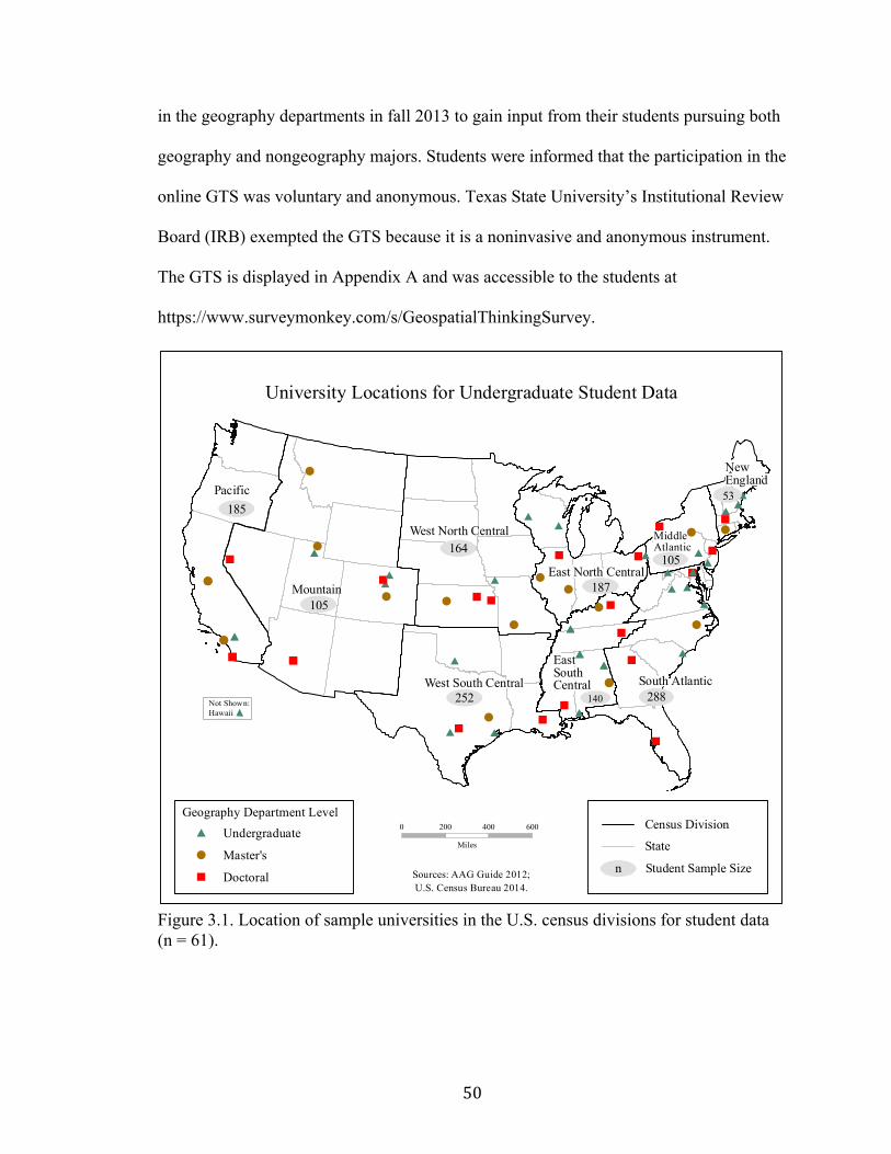
50

in the geography departments in fall 2013 to gain input from their students pursuing both

geography and nongeography majors. Students were informed that the participation in the

online GTS was voluntary and anonymous. Texas State University’s Institutional Review

Board (IRB) exempted the GTS because it is a noninvasive and anonymous instrument.

The GTS is displayed in Appendix A and was accessible to the students at

https://www.surveymonkey.com/s/GeospatialThinkingSurvey.

Figure 3.1. Location of sample universities in the U.S. census divisions for student data (n = 61).

Pacific

Mountain

West North Central

West South Central

East South Central

East North Central

South Atlantic

Middle Atlantic

New England

#"

!"

!

"

!

#

"

" "

!

!

#

""

!!

##

#

""!

#

# #

"

"

"

!

#

#

#

#

"

"

!

#

#

#

# #

#

#

"!

###

"

"

!

!

#

#

"

!

!

#

!

##

#

""

!

!

#

University Locations for Undergraduate Student Data

164

105187

252

105

185

140 288

53

0 200 400 600

Miles

Not Shown: Hawaii

Geography Department Level# Undergraduate

! Master's

" Doctoraln Student Sample Size

Census Division

State

Sources: AAG Guide 2012; U.S. Census Bureau 2014.

51

Table 3.1. Distribution and Number of Undergraduate Students Who Completed the Geospatial Thinking Survey (GTS) by Census Division (Number of Universities).

Census Divisions Geography Department Level

Total Doctoral Departments

Master’s Departments

Undergraduate Departments

South Atlantic 36 (3) 138 (1) 113 (6) 287 (10) West South Central 131 (2) 25 (1) 97 (3) 253 (6) East North Central 22 (2) 36 (2) 133 (3) 191 (7) Pacific 142 (1) 19 (2) 24 (2) 185 (5) West North Central 113 (2) 38 (2) 13 (1) 164 (5) East South Central 41 (3) 19 (2) 76 (4) 136 (9) Mountain 41 (3) 43 (3) 21 (3) 105 (9) Middle Atlantic 9 (2) 70 (1) 26 (2) 105 (5) New England 9 (1) 17 (1) 27 (3) 53 (5) Total 544 (19) 405 (15) 530 (27) 1479 (61)

From across the country, 1573 students in 32 states completed the GTS online in

the fall 2013 semester. The sample included a few graduate, international, private

university, or community college students, and also some invalid responses. So, such

cases were not included in the analyses as the focus of this dissertation research is

undergraduate students in public universities in the United States. After discarding the 94

unusable cases from the sample, the total sample size became 1479 (Table 3.1).

Characteristics of the Test Instrument

A dearth of standardized tests of geospatial thinking exists in the literature (NRC

2006; Lee and Bednarz 2009; Huynh and Sharpe 2009, 2013). As the basis of the GTS, I

used questions from the Spatial Thinking Ability Test (STAT) developed and used by

Lee (2005), endorsed by the Association of American Geographers (AAG 2006), and

employed by Lee and Bednarz (2009, 2012). The STAT has 16 spatial thinking questions.

I omitted the four geometric spatial thinking questions as they are not geospatial. I

excluded a map navigation or way-finding question because of repetition and a question

on 3-D image visualization because it resulted in low reliability in the pilot study

52

conducted in fall 2012. Therefore, ten geospatial thinking questions, some modified for

syntax and better student understanding, from the STAT were included in the GTS.

Geospatial thinking consists of several different components. Table 3.2 outlines the

Table 3.2. Geospatial Thinking Domains in the Geospatial Thinking Survey (GTS): Based on Golledge (1995, 2002); Gersmehl and Gersmehl (2006); Jo and Bednarz (2009); and Lee and Bednarz (2012).

Geospatial Thinking Domain/

Component

Description NRC (2006); Jo and Bednarz (2009)

Taxonomy

GTS Question

1. Geospatial Pattern and Transition

Discerning geospatial patterns; graphing geospatial transitions; comparing and transferring map information to graphic information

Cell 23: Complex-spatial concept; using tool of representation; reasoning at processing level

1

2. Direction and Orientation

Map navigation; way-finding; route planning; comprehending orientation and direction

Cell 17: Simple-spatial concept; using tool of representation; reasoning at processing level

2

3. Geospatial Profile and Transition

Recognizing geospatial form; imagining a slope profile based on a topographic/contour map; transforming perceptions, representations, and images from one dimension to another; graphing a geospatial transition

Cell 24: Complex-spatial concept; using tool of representation; reasoning at output level

3

4. Geospatial Association and Transition

Correlating geospatially distributed phenomena; identifying geospatial correlation between maps; assessing geospatial association; making geospatial comparisons; graphing geospatial transitions


4 (Geospatial Association

and Transition),

5 (Geospatial

Assoc.) 5. Geospatial Shapes

Identifying and comprehending integration of geographic features represented as points, lines (networks), areas/polygons (regions)

Cell 17: Simple-spatial concept; using tool of representation; reason-ing at processing level

6, 7, 8, 9

6. Geospatial Overlay

Comprehending overlaying, aggregating, and dissolving map layers to choose the best location based on various spatial/ geographical conditions, connections, distance; inferring a geospatial aura (influence)


10

53

geospatial thinking domains encompassed by the GTS. These domains are based on the

components given by such scholars as Golledge (1995, 2002), Gersmehl and Gersmehl

(2006), Jo and Bednarz (2009), and Lee and Bednarz (2012). The GTS also included

demographic, geographic, and academic background questions.

Reliability and Validity

To identify flaws in the instrument, I conducted a pilot study with undergraduate

students in geography undergraduate general education courses at Texas State University

in the fall 2012 semester. I invited pilot study participation to undergraduate students by

visiting five geography undergraduate level classes. Participation was voluntary and

anonymous. Using the Survey Monkey program, 77 undergraduate students completed

the GTS online in the pilot study. The pilot study showed that students took about ten-

fifteen minutes, on average, to complete the GTS, thereby demonstrating that students did

not need an inordinate amount of time to complete the GTS. The results of the pilot study

revealed statistically significant differences among the mean scores of the various

categories of ethnicity, academic major, academic classification, and academic

experience in geography (number of college geography courses taken). No statistically

significant differences were found among the mean scores of the various categories of

age, sex, highest educational attainment of parents (socioeconomic status), annual income

of parents (socioeconomic status), and urban/rural location (geographic location). Thus,

ethnicity and academic background influenced geospatial thinking of students, while age,

sex, socioeconomic status, and geographic location did not influence geospatial thinking

of students in the exploratory study with a small sample of size of 77 undergraduate

students at one university.

54

To establish the internal consistency of the GTS, I calculated the Cronbach’s

Alpha statistic that measures the intercorrelation of items, that is, the extent to which item

responses obtained at the same time correlate with each other (Lee and Bednarz 2012).

The Cronbach’s Alpha for the GTS was 0.679, which signifies a low level of internal

consistency in social science research. However, the results of the pilot study indicated

that if one particular question (3-d terrain question) were removed from the GTS, the

Cronbach’s Alpha would increase to 0.708, a value indicating an acceptable level of

internal consistency among the items. Out of a total of 77 students in the pilot study, only

20 answered the 3-d terrain question correctly. I, therefore, deleted this question from the

GTS in the final administration for this dissertation. Spatial thinking consists of multiple

components/domains that are not correlated to each other (Voyer, Voyer, and Bryden

1995; Gersmehl and Gersmehl 2006; Smith 2007; Lee and Bednarz 2012; Gersmehl

2012; Huynh and Sharpe 2013; Ishikawa 2013; Sinton et al. 2013), leading to lower

internal consistency among the test items.

Validity is considered to be the degree to which the test measures what it claims

to measure. Validity shows how well the test instrument reflects the real meaning of the

investigated concepts, examined through face and content validity (Huynh and Sharpe

2013). The GTS has face validity because it measures geospatial thinking skills using

maps and geographic information. Content validity relates to what extent the test items

represent the concepts of interest (Huynh and Sharpe 2013). The GTS has content

validity as it covers a representative sample of the geospatial thinking skills discussed in

the literature. Thus, GTS is a reliable and valid test of geospatial thinking skills; of

course, as mentioned, the GTS drew its questions from the AAG’s STAT (2006).

55

Domains of Geospatial Thinking

I employed principal components analysis (PCA) to group GTS questions into

distinct geospatial thinking domains. PCA analysis verified the grouping of GTS

questions into different components with the domains identified in the literature.

Quantitative Analyses

Variables

The dependent variable in my study is geospatial thinking, measured by score on

the GTS. The maximum possible score on the GTS is ten for a total of ten geospatial

thinking questions. The minimum score on the GTS is zero, if a student answered all the

questions incorrectly.

The 12 independent/predictor variables are grouped into three broad categories:

1. Demographic variables: sex, age, ethnicity, parents’ annual income (a measure of

socioeconomic status), and highest educational attainment of parents (a measure of

socioeconomic status)

2. Academic variables: academic classification, academic major, number of

geography courses taken at the high school level (a measure of formal academic

experience in geography), number of geography courses taken at the college level (a

measure of formal academic experience in geography), and geography department level

(at a student’s current university)

3. Geographic location variables: urban/suburban/rural patterns (where the students

grew up), and census division (in which the student’s current university is located)

Students with non-geography majors are the control group, and the students who

are geography majors are the experimental group. Taking geography courses is expected

56

to act as an intervention to improve geospatial thinking. The research therefore examines

whether geography courses improve geospatial thinking in students.

Student Performance Measured by GTS Score: Geospatial Thinking Index (GTI)

I assigned students a level on Geospatial Thinking Index (GTI), based on GTS

score. This index assigned students into three categories with an overall geospatial

thinking level based on competency on the GTS, using standard deviation method. The

three categories identified are:

1. Low Geospatial Thinking Level

2. Medium Geospatial Thinking Level

3. High Geospatial Thinking Level

Group Differences on GTS Score Means

I employed a t-test and a one-way analysis of variance (ANOVA) to interpret

group differences in geospatial thinking of students from various backgrounds. The t-test

and ANOVA are parametric tests that assume the data being analyzed are normally

distributed (Monday, Klein, and Lee 2005). The GTS scores are approximately normally

distributed.

The t-test determines if two categories of data are significantly different from

each other. I used the t-test for only one independent variable—sex—to compare mean

scores of female and male students. ANOVA analyzes means on a quantitative Y

dependent variable across two or more groups of X independent variables (Explorable

2013; Park 2009). I ran 11 ANOVAs for 11 independent variables to compare the means

of categories of different variables for statistical significance. I used the Games-Howell

test (a post-hoc comparison method that does not assume homogeneity of variances or

57

equal sample sizes) to find internal group differences for significant ANOVA runs,

thereby determining which groups differ and by which degree (Laerd Statistics 2014).

Geospatial Thinking Score Prediction

I employed multiple regression model to explain which independent variables are

significant predictors of the dependent variable—geospatial thinking. Multiple regression,

concerning the association of two or more independent variables (taken together) with

one dependent variable, compares one group to another to show which variables

contribute best to explain/predict the dependent variable (Brace, Kemp, and Snelgar

2012).

To predict the level of geospatial thinking of a student from a particular

background (a combination of different demographic, academic, or geographic variables),

I applied a predictive model in the analyses. This model, called the Geospatial Thinking

Model (GTM), along with the regression model, is helpful in anticipating geospatial

thinking acumen of students who do not take the GTS. These predicted GTS scores are

based on such student background information as belonging to a particular ethnic group

or undertaking an academic major. For this predictive model, I employed the Cubist

software, a data mining and artificial intelligence tool for generating rule-based predictive

models from data.

Student Performance on Individual Questions of the GTS

I analyzed the performance of all students on individual GTS questions based on

the percentage of students answering a particular question correctly. I divided the GTS

questions into three categories—Less Difficult, Difficult, and More Difficult, based on

what percentage of students answered the question correctly and incorrectly.

58

Group Differences on Individual Questions of the GTS

The chi-square test of independence is a non-parametric method used to

determine whether there is an evidence of a significant association between two

categorical variables (Daniel 1990; Stat Trek 2014). I used the chi-square test of

independence to investigate the relationship between each independent variable

(categorical variable) and each geospatial thinking domain (distinct GTS questions with

students’ responses coded dichotomously, i.e. categorical), and to interpret group

differences in different geospatial thinking domains of students from various

backgrounds. I ran chi-square to analyze whether differences in one variable are

associated to understanding a geospatial thinking domain correctly or incorrectly.

Qualitative Analyses

I conducted telephone interviews with 27 geography instructors, three each from

nine census divisions, employing convenience and stratified sampling. From each census

division, I interviewed geography faculty from three department levels each—doctoral,

master’s, and undergraduate—to gauge the geospatial concepts that the students find

difficult to understand based on the instructors’ perception. The interviews were semi-

structured with two demographic questions about instructors’ sex and ethnicity, two

contextual questions about instructor experience, and four open-ended questions about

geospatial thinking of undergraduate students and classroom activities. Based on the

instructors’ responses on the qualitative interviews, I undertook an analysis of the

geospatial concepts using content analysis.

59

Mixed-method Analysis

My dissertation research brought together the quantitative and qualitative datasets

to determine if the two matched. Student performance on the GTS provided the

quantitative data (GTS scores), and instructor perception in the interviews contributed the

qualitative data. I searched for trends in the two datasets, to confirm if the instructors’

perceptions about students’ understanding of different geospatial concepts verify student

performance on various geospatial thinking domains. I also looked for mismatches

between the two datasets to formulate follow-up questions as to why the datasets do not

correspond.

60

CHAPTER IV

QUANTITATIVE ANALYSES AND FINDINGS

Domains of Geospatial Thinking

Principal component analysis (PCA), a method of factor analysis, was employed

to see if GTS questions group into a more coherent set of geospatial thinking

components/domains. Factor analysis identifies the minimum underlying factors needed

to explain the intercorrelations among the test items (Lee and Bednarz 2012). To verify

the skills tested by the six domains as separate components of geospatial thinking (Table

3.2), the PCA results should yield similar components to reflect the six domains. I

subjected responses to the 10-item GTS to PCA in Statistical Package for the Social

Sciences (SPSS) software. The PCA groupings were based on students’ responses to the

GTS questions. PCA revealed four components with eigenvalues greater than 1.0,

accounting for 48.31 percent of cumulative variance, with component loadings given by

varimax rotation (Table 4.1).

GTS questions and corresponding factor loadings are presented in Table 4.1. In

interpreting the rotated factor pattern, a question was said to load on a given component if

the factor loading was 0.40 or greater for that component, and was less than 0.40 for the

other (Stevens 1986; Lee and Bednarz 2012; SAS 2014). Using this criterion, four

questions were found to load on Component I, two questions each on Components II and

III, and one question on Component IV.

61

Table 4.1 Results of Principal Component Analysis (PCA) for the GTS. GTS Question Number and Geospatial

Thinking Domain Components

I II III IV 1 (Geospatial Pattern and Transition) -0.593 0.051 0.143 0.136 2 (Geospatial Direction and Orientation) -0.144 0.031 0.782 0.045 3 (Geospatial Profile and Transition) 0.386 -0.322 0.185 0.263 4 (Geospatial Association and Transition) 0.035 0.775 0.138 -0.148 5 (Geospatial Association) 0.146 -0.180 0.545 -0.016 6 (Geospatial Shapes) 0.720 -0.097 0.057 0.146 7 (Geospatial Shapes) 0.480 0.338 -0.017 0.241 8 (Geospatial Shapes) 0.563 0.001 0.159 -0.194 9 (Geospatial Shapes) 0.187 -0.499 0.205 -0.364 10 (Geospatial Overlay) -0.011 -0.049 0.043 0.829 Eigenvalues 1.701 1.079 1.038 1.012 % of variance 17.007 10.792 10.384 10.123 Cumulative % of variance 17.007 27.800 38.184 48.307

Table 4.1 shows that Q6 (question 6), Q7, and Q8 loaded on Component I, all

three questions representing Geospatial Shapes, identified in the literature as a distinct

domain (Table 3.2), and a discrete component in the PCA results (Table 4.1). However,

Q9 is also part of the same Geospatial Shapes domain in Table 3.2, but was not identified

by the PCA for Component I. Q1 (Geospatial Pattern and Transition domain) is also

loaded on component I but is not part of the same Geospatial Shapes domain. The PCA

thus produced partially meaningful results in relation to component I. Also, Q1 has an

inverse relationship with questions 6, 7, and 8. For example, students answering Q1

correctly are more likely to answer questions 6, 7, and 8 incorrectly, and vice-versa.

Q4 represents the Geospatial Association and Transition domain in the literature

and a discrete Component II by PCA results. Although both Q4 and Q5 are part of the

Geospatial Association domain, the PCA found only Q4 as distinct in Component II.

However, Q4 assesses both Geospatial Association and Transition, while Q5 only focuses

on Geospatial Association. Q9 that loaded on component II is in the Geospatial Shapes

62

domain. However, questions 4 and 9 are inversely related to each other based on

students’ responses.

Q2 loaded on component III, identified in the Direction and Orientation domain

and a distinct component III in the PCA results. Q5 representing the Geospatial

Association domain, also loaded on Component III. Q2 and Q5 are therefore not part of

the same domain, but they loaded on Component III.

Q10, characterizing the Geospatial Overlay domain, loaded on component IV in

the PCA results. The PCA did not select Q3 as a separate Geospatial Profile and

Transition domain.

Thus, the four components produced by PCA do represent four distinct geospatial

thinking domains—Geospatial Shapes, Geospatial Association and Transition, Direction

and Orientation, and Geospatial Overlay. Although Geospatial Shapes and Geospatial

Association and Transition were separate components, they did not include all

representative questions.

Lee and Bednarz (2012) presented similar question grouping results for STAT,

where group inclusion for some questions were not clear and meaningful as were those

not selected for any group. These outcomes demonstrate some questions may not be

adequately worded. Some questions represent more than one domain of geospatial

thinking. Ten questions, further, covered by six domains (in the case of GTS) are not

sufficient to capture the entire range of geospatial thinking skills. Researchers thus need

to develop more comprehensive assessments and tests to measure geospatial thinking.

Indeed, both the STAT and GTS omit such fundamental geospatial thinking skills as

scale, frames of reference, regionalization (spatial classification), spatial diffusion, spatial

63

hierarchy, and spatial analog. Huynh and Sharpe’s (2013) geospatial thinking assessment

includes questions on scale, frames of reference (latitude and longitude), spatial

enclosure, and spatial diffusion. Their 30-question instrument, however, was very long

requiring about 45 minutes for completion. The instrument also included drawing and

short answer writing questions, which are not feasible for a national survey conducted

online. Scoring drawing and writing questions is subjective and complicated. A

geospatial thinking test that comprehensively measures a wide range of skills within a

reasonable number of objective questions for a national online administration remains

elusive.

Student Performance Measured by GTS score: Geospatial Thinking Index (GTI)

Students’ score on the GTS is a measure of their geospatial thinking. Based on the

ten geospatial thinking questions, a student’s score may vary between 0 and 10 on the

GTS. The mean score of students on the GTS was 6.57, with a standard deviation of 2.00,

and the mode score was 8. Table 4.2 displays the number of students obtaining GTS

scores from 0 to 10.

Table 4.2. GTS Scores and Student Frequencies. GTS Score Number of Students Percent of Students Cumulative Percentage

0 5 0.3 0.3 1 13 0.9 1.2 2 49 3.3 4.5 3 75 5.1 9.6 4 94 6.4 16.0 5 147 9.9 25.9 6 225 15.2 41.1 7 314 21.2 62.3 8 324 21.9 84.2 9 203 13.7 97.9 10 30 2.1 100.0

Total 1479 100.0

64

The distribution of the GTS scores is approximately normal, though slightly

negatively skewed (Figure 4.1). This implies that the majority of students performed at a

similar level, and most students answered over half of the questions correctly. A sizeable

proportion of students performed both above and below average. Thus, the GTS as an

assessment instrument appropriately differentiates levels of geospatial thinking from

basic through intermediate to an advanced level of performance. Huynh and Sharpe

(2013) found similar results for 104 students as assessed via geospatial thinking

assessment.

Figure 4.1. Histogram of student performance on the GTS.

Huynh and Sharpe (2013) categorized the students into novice, intermediate, and

expert levels to investigate a measurable or identifiable development of mature geospatial

65

thinking, utilizing a standard deviation method to assign students to one of the three

expertise levels on the geospatial thinking assessment. The researchers used standard

scores of one standard deviation above and below the mean for the critical values

between different expertise levels.

Following Huynh and Sharpe (2013), I also categorized students into three levels

of geospatial thinking using the standard deviation technique. I grouped students relative

to the mean of the distribution (6.57), with the standard scores of one standard deviation

(2.00) above and below the mean producing the three class intervals. Students with GTS

scores greater than one standard deviation above the mean (greater than 8.6) were

classified as students with high geospatial thinking level, those with GTS scores one

standard deviation less than the mean (less than 4.6) were classified as students with low

geospatial thinking level, and those within standard deviation of the mean (from 4.6 to

8.6) were classified as students with medium geospatial thinking level (Table 4.3). Using

the 1479 student scores, ANOVA confirmed differences among three levels of

performance were significant (F = 2465.46, p <0.001).

Table 4.3. Geospatial Thinking Index. Geospatial Thinking

Level GTS Score

Range Number of

Students (%) Mean Score

Low 0-4 236 (16.0) 3.02 Medium 5-8 1010 (68.3) 6.81 High 9-10 233 (15.7) 9.13 Total 0-10 1479 (100) 6.57

Group Differences on GTS Score Means

I used t-test (alpha = 0.05) in SPSS to interpret group differences in geospatial

thinking for only one independent variable—sex. I ran 11 ANOVAs (alpha = 0.05) for

each of the 11 predictor variables to compare the means of categories of different

66

variables (e.g. white, Hispanic, black, and Asian for ethnicity) for statistical significance.

After running the ANOVA tests, I used the Games-Howell test (a post-hoc comparison

method that does not assume homogeneity of variances or equal sample sizes) to find

internal group differences, thereby determining which groups differ and by which degree

(Laerd Statistics 2014).

Table 4.4 presents the distribution of GTS score means for females and males.

The t-test found a statistically significant difference between the mean scores of females

and males in which the mean score of male students is higher than the mean score of

female students. Sex thus influences the geospatial thinking of students.

Table 4.4. GTS Score Means for Sex.

Sex Number of Students (%)

Total Possible

Score

Highest Score

Lowest Score

Mean Score

t-test

p Value

Female 804 (54.4) 10 10 0 6.33 -4.955 <0.001 Male 675 (45.6) 10 10 0 6.85

Total 1479 (100) 10 10 0 6.57

Age generally reflects growing life experiences. Table 4.5 summarizes the

distribution of students in three age groups. The ANOVA found a statistically significant

difference among the mean scores of three age categories. The mean score of students 21-

24 years old and more than 24 years old is highest, while that of 18-20 years old students

is lowest. Increasing age thus has a positive effect on students’ geospatial thinking.

Table 4.5. GTS Score Means for Age Categories.

Age Number of Students (%)

Total Possible

Score

Highest Score

Lowest Score

Mean Score F p

Value

18-20 751 (50.8) 10 10 0 6.28

15.988 <0.001 21-24 473 (32.0) 10 10 0 6.87 > 24 255 (17.2) 10 10 0 6.86 Total 1479 (100) 10 10 0 6.57

67

Post-hoc comparisons (alpha = 0.05) in Table 4.6 show that 18-20 year old

students scored significantly lower than both students 21-24 years old and more than 24

years old. Older students therefore perform better in geospatial thinking skills.

Table 4.6. Post-hoc Comparisons (Games-Howell) of GTS Score by Age Categories (p Value in Parentheses).

Age 18-20 21-24 21-24 -0.586 (<0.001) > 24 -0.578 (<0.001) 0.008 (0.998)

Table 4.7 presents the distribution of four ethnic groups in the data. The ANOVA

found a statistically significant difference among the mean scores of four ethnic

categories. The mean score of white students is highest, while that of black students is

lowest. Ethnicity affects the geospatial thinking of students.

Table 4.7. GTS Score Means for Ethnic Groups.

Ethnicity Number of Students

(%)

Total Possible

Score

Highest Score

Lowest Score

Mean Score F p

Value

White 1103 (74.6) 10 10 0 6.89

51.732 <0.001 Hispanic 136 (9.2) 10 10 1 5.86 Black 127 (8.6) 10 10 0 4.87 Asian 113 (7.6) 10 10 1 6.20 Total 1479 (100) 10 10 0 6.57

Post-hoc comparisons in Table 4.8 shows white students scored significantly

higher than Hispanic, black, and Asian students. Both Hispanic and Asian students scored

significantly higher than black students. But the difference between the scores of

Hispanic and Asian students is not statistically significant. Ethnicity therefore affects

students’ geospatial thinking.

68

Table 4.8. Post-hoc Comparisons (Games-Howell) of GTS Score by Ethnic Groups (p Value in Parentheses). Ethnicity White Hispanic Black Hispanic 1.028 (<0.001) Black 2.022 (<0.001) 0.994 (0.002) Asian 0.685 (0.004) -0.343 (0.577) -1.337 (<0.001)

The ANOVA found a statistically significant difference among the mean scores of

four categories of the annual income of parents (Table 4.9). The mean score of students

from high-income groups (>$75,000) is highest. Socioeconomic status (annual income of

parents) influences geospatial thinking of students.

Table 4.9. GTS Score Means for Parents’ Annual Income Categories. Annual

Income of Parents

Number of Students (%)

Total Possible

Score

Highest Score

Lowest Score

Mean Score F p

Value

<$25,000 223 (15.1) 10 10 1 6.38

7.679 <0.001

$25,000-$50,000 351 (23.7) 10 10 0 6.21

$51,000-$75,000 333 (22.5) 10 10 0 6.65

>$75,000 572 (38.7) 10 10 0 6.81 Total 1479 (100) 10 10 0 6.57

Post-hoc comparisons (Table 4.10) for income groups showed that the students

from the second income category ($25,000-$50,000) scored significantly lower than

students from third ($51,000-$75,000) and fourth (>$75,000) categories, yet the third and

fourth income groups were not significantly different. Higher income groups may mean

higher geospatial thinking but not necessarily across all income categories. Post-hoc

comparison does not reveal any pattern or important decreasing or increasing differences

in geospatial thinking across income categories.

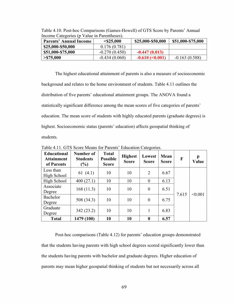
69

Table 4.10. Post-hoc Comparisons (Games-Howell) of GTS Score by Parents’ Annual Income Categories (p Value in Parentheses). Parents’ Annual Income <$25,000 $25,000-$50,000 $51,000-$75,000 $25,000-$50,000 0.176 (0.781) $51,000-$75,000 -0.270 (0.450) -0.447 (0.013) >$75,000 -0.434 (0.060) -0.610 (<0.001) -0.163 (0.588)

The highest educational attainment of parents is also a measure of socioeconomic

background and relates to the home environment of students. Table 4.11 outlines the

distribution of five parents’ educational attainment groups. The ANOVA found a

statistically significant difference among the mean scores of five categories of parents’

education. The mean score of students with highly educated parents (graduate degrees) is

highest. Socioeconomic status (parents’ education) affects geospatial thinking of

students.

Table 4.11. GTS Score Means for Parents’ Education Categories. Educational Attainment of Parents

Number of Students

(%)

Total Possible

Score

Highest Score

Lowest Score

Mean Score F p

Value

Less than High School 61 (4.1) 10 10 2 6.67

7.615 <0.001

High School 400 (27.1) 10 10 0 6.13 Associate Degree 168 (11.3) 10 10 0 6.51

Bachelor Degree 508 (34.3) 10 10 0 6.75

Graduate Degree 342 (23.2) 10 10 1 6.83

Total 1479 (100) 10 10 0 6.57

Post-hoc comparisons (Table 4.12) for parents’ education groups demonstrated

that the students having parents with high school degrees scored significantly lower than

the students having parents with bachelor and graduate degrees. Higher education of

parents may mean higher geospatial thinking of students but not necessarily across all

70

categories. Post-hoc comparison does not reveal any pattern or important decreasing or

increasing differences in geospatial thinking across parents’ education categories.

Table 4.12. Post-hoc Comparisons (Games-Howell) of GTS Score by Parents’ Education Categories (p Value in Parentheses).

Parents’ Education

Less than High School High School Associate

Degree Bachelor Degree

High School 0.547 (0.311)

Associate Degree 0.166 (0.983) -0.381 (0.280)

Bachelor Degree -0.074 (0.999) -0.621 (<0.001) -0.240 (0.670)

Graduate Degree -0.161 (0.979) -0.708 (<0.001) -0.327 (0.436) -0.087 (0.966)

Increasing academic classification reflects higher-level formal classroom

instruction. Table 4.13 displays the distribution of students in four academic

classifications. The ANOVA found a statistically significant difference among the mean

scores of four academic classifications. The mean score of senior (fourth-year) students is

highest, while that of freshmen (first-year) is lowest. Similar to age, higher academic

classification thus positively affects students’ geospatial thinking.

Table 4.13. GTS Score Means for Academic Classifications.

Academic Classification

Number of

Students (%)

Total Possible

Score

Highest Score

Lowest Score

Mean Score F p

Value

Freshman (First Year)

268 (18.1) 10 10 0 6.19

22.023 <0.001

Sophomore (Second Year)

366 (24.7) 10 10 1 6.23

Junior (Third Year)

401 (27.1) 10 10 0 6.44

Senior (Fourth Year)

444 (30.1) 10 10 0 7.18

Total 1479 (100) 10 10 0 6.57

71

Post-hoc comparisons (Table 4.14) for academic classifications revealed that

senior students scored significantly higher than freshman, sophomore, or junior students.

Similar to the oldest age group, the highest level of academic classification affects the

level of geospatial thinking.

Table 4.14. Post-hoc Comparisons (Games-Howell) of GTS Score by Academic Classifications (p Value in Parentheses).

For academic major question on the GTS, students responded with more than 100

academic majors. I categorized the academic majors into categories of related majors to

make comparisons easier. An academic major category with more than 30 respondents

kept its distinct category. I grouped academic majors with less than 30 respondents into

larger groups based on academic college affiliation. For example, 37 students reported

history as their academic major; history was then identified as a separate major.

However, both anthropology and sociology had less than 30 respondents each, thereby

placing them into the category termed Other Social Science Majors. Some of the other

academic majors grouped into the Other Social Science Majors category included

economics, international studies, political science, social work, public administration, and

philosophy. Some of the academic majors categorized in the Other Science Majors

category included chemistry, physics, mathematics, meteorology, neuroscience,

radiology, forestry, and astronomy. Art, music, theatre, film, dance, photography, interior

design, linguistics, English, French, Japanese, and Spanish are some of the academic

majors grouped into the Humanities Majors category.

Academic Classification Freshman Sophomore Junior

Sophomore -0.045 (0.993) Junior -0.251 (0.410) -0.206 (0.515) Senior -0.994 (<0.001) -0.950 (<0.001) -0.743 (<0.001)

72

Table 4.15 exhibits the distribution of students in 18 academic major groups,

arranged according to decreasing mean scores. The ANOVA found a statistically

significant difference among the mean scores of different academic majors. The mean

score of geography majors is the highest, while that of criminal justice majors is the

lowest. Academic major thus shapes students’ geospatial thinking.

Table 4.15. GTS Score Means for Academic Majors.

Academic Major

Number of Students

(%)

Total Possible

Score

Highest Score

Lowest Score

Mean Score F p

Value

Geography 367 (24.8) 10 10 2 7.57

15.10 <0.001

Geology 31 (2.1) 10 10 5 7.48 Environmental Science 59 (4.0) 10 10 1 7.20

Other Science Majors 66 (4.5) 10 10 4 7.15

Biology 57 (3.8) 10 10 3 7.02 Engineering 50 (3.4) 10 10 1 6.96 History 37 (2.5) 10 9 2 6.81 Computer Science 36 (2.4) 10 9 2 6.58

Humanities Majors 50 (3.4) 10 9 1 6.56

Psychology 46 (3.1) 10 9 1 6.15 Other Social Science Majors 138 (9.3) 10 10 0 6.07

No Major 45 (3.1) 10 9 0 6.02 Business 165 (11.2) 10 10 2 6.00 Health 51 (3.4) 10 10 1 5.82 Nursing 40 (2.7) 10 9 0 5.70 Education 136 (9.2) 10 10 0 5.62 Communication 67 (4.5) 10 9 1 5.54 Criminal Justice 38 (2.6) 10 10 1 5.29

Total 1479 (100) 10 10 0 6.57

Table 4.16 displays the significant post-hoc comparisons for 18 academic major

groups. Both geography and geology students scored higher than nursing, health,

psychology, criminal justice, education, communication, business, Other Social Science

73

Majors, and No Major students. Students in Other Science Majors scored higher than

education, communication, business, criminal justice, nursing, health, and Other Social

Science Majors students. Biology students scored higher than education, communication,

business, and criminal justice students. Engineering students scored higher than

education, communication, and criminal justice students. Environmental science students

scored higher than education, communication, business, criminal justice, and Other

Social Science Majors students. Education, communication, and criminal justice students

scored lower than geography, geology, engineering, environmental science, biology, and

Other Science Majors students. Business students scored lower than geography, geology,

environmental science, biology, and Other Science Majors students. Other Social Science

Table 4.16. Significant Post-hoc Comparisons (Games-Howell) of GTS Score by Academic Majors (p Value in Parentheses).

Academic Majors

Geog-raphy

Geol-ogy

Envt. Sci.

Other Science Biology Engine-

ering Health Nursing

Other Science -1.328

(.041) -1.452 (.039)

Psycho-logy

1.417 (.001)

1.332 (.029)

Other Social Science

1.504 (<.01)

1.419 (.001)

1.138 (.029)

1.086 (.008)

No Major 1.547 (.001)

1.462 (.023)

Business 1.569 (<.01)

1.484 (<.01)

1.203 (.006)

1.152 (.001)

1.018 (.012)

Health 1.746 (<.01)

1.660 (.005) 1.328

(.041)

Nursing 1.869 (<.01)

1.784 (.005) 1.452

(.039)

Educa-tion

1.952 (<.01)

1.866 (.<01)

1.586 (<.01)

1.534 (<.01)

1.400 (<.01)

1.342 (.004)

Commun-ication

2.032 (<.01)

1.947 (<.01)

1.666 (.001)

1.614 (<.01)

1.480 (.002)

1.423 (.018)

Criminal Justice

2.280 (<.01)

2.194 (.001)

1.914 (.006)

1.862 (.004)

1.728 (.013)

1.671 (.037)

74

Majors students scored lower than geography, geology, environmental science, and Other

Science Majors. Nursing and health students scored lower than geography, geology, and

Other Science Majors students.

Table 4.17 presents the distribution of students with different academic

experience in high school geography, measured by number of geography courses studied

in high school. The ANOVA found a statistically significant difference among the mean

scores of different high school geography levels. The mean score of students who studied

no geography course at the high school level is the highest, while that of students who

studied two geography courses is the lowest. This outcome is certainly perplexing.

Table 4.17. GTS Score Means for Number of High School Geography Courses. Number of

High School Geography

Courses

Number of

Students (%)

Total Possible

Score

Highest Score

Lowest Score

Mean Score F p

Value

No Geography Course

507 (34.3) 10 10 1 6.79

3.639 0.012

1 Geography Course

656 (44.3) 10 10 0 6.51

2 Geography Courses

210 (14.2) 10 10 1 6.33

>2 Geography Courses

106 (7.2) 10 10 0 6.37

Total 1479 (100) 10 10 0 6.57

Post-hoc comparisons (Table 4.18) for the number of high school geography

courses taken showed that students who never studied a geography course in high school

scored significantly higher than students who studied two geography courses. All other

differences were not statistically significant. This outcome may add to the general

assertion by some scholars (Sinton et al. 2013) and educational policymakers that

75

geography is not properly taught in high schools in the U.S., in this case regarding

geospatial thinking skills.

Table 4.18. Post-hoc Comparisons (Games-Howell) of GTS Score by Number of High School Geography Courses (p Value in Parentheses).

Table 4.19 shows the distribution of students with different academic experience

in college geography, measured by number of geography courses studied. The ANOVA

found a statistically significant difference among the mean scores of students who had

taken various numbers of college geography courses. The mean score of students who

had taken more than five college geography courses is the highest, while those students

who had taken no college geography scored the lowest. College geography courses

bolster students’ geospatial thinking, thereby corroborating that geography academic

majors have the highest level of geospatial thinking (Tables 4.15 and 4.16).

Table 4.19. GTS Score Means for the Number of College Geography Courses. Number of

College Geography

Courses

Number of

Students (%)

Total Possible

Score

Highest Score

Lowest Score

Mean Score F p

Value

No Geography Course

253 (17.1) 10 10 0 6.10

44.932 <0.001

1-2 Geography Courses

812 (54.9) 10 10 0 6.27


161 (10.9) 10 10 2 7.00

>5 Geography Courses)

253 (17.1) 10 10 4 7.72

Total 1479 (100) 10 10 0 6.57

High School Geography No Geography Course

1 Geography Course

2 Geography Courses

1 Geography Course 0.283 (0.071) 2 Geography Courses 0.460 (0.031) 0.178 (0.694) >2 Geography Courses 0.421 (0.248) 0.138 (0.925) -0.039 (0.999)

76

Post-hoc comparisons (Table 4.20) for the number of college geography courses

taken showed students with no experience in college geography courses scored

significantly lower than students who had taken three or more college geography courses.

Students who had taken more than five college geography courses scored significantly

higher than students who had taken no, 1-2, or 3-5 college geography courses. Studying

geography in college is thus very important in improving geospatial thinking.

Table 4.20. Post-hoc Comparisons (Games-Howell) of GTS Score by Number of College Geography Courses (p Value in Parentheses).

Undergraduate students responding in this study were from geography

departments granting highest degree at three levels—undergraduate, master’s, and

doctoral. Table 4.21 displays the distribution of students in three geography department

degree levels. The ANOVA revealed no statistically significant difference among the

Table 4.21. GTS Score Means for Geography Department Degree Levels.

Geography Department

Level

Number of

Students (%)

Total Possible

Score

Highest Score

Lowest Score

Mean Score F p

Value

Doctoral 544 (36.8) 10 10 1 6.50

0.895 0.409 Master’s 405

(27.4) 10 10 0 6.68

Undergraduate 530 (35.8) 10 10 0 6.55

Total 1479 (100) 10 10 0 6.57

Number of College Geography Courses

No Geography Course



1-2 Geography Courses -0.170 (0.672)

3-5 Geography Courses -0.901 (<0.001) -0.732 (<0.001)

>5 Geography Courses -1.625 (<0.001) -1.455 (<0.001) -0.723 (<0.001)

77

mean scores of students from the three geography department degree levels. Although

geography studied at the college level makes a positive difference in undergraduate

students’ geospatial thinking, undergraduate student performance is similar regardless of

whether geography departments offer graduate degrees.

Urban, suburban, or rural patterns reflect geographic locations where the students

grew up. The role of the structure of cities, suburbs, and rural areas in shaping students’

spatial and geospatial thinking has not been expressed in the literature. Table 4.22

outlines the distribution of students who grew up in urban/suburban/rural areas. The

ANOVA found a statistically significant difference among the mean scores of students

from urban/suburban/rural areas. The mean score of rural students is highest, and that of

urban students is lowest. Urban/suburban/rural patterns steer students’ geospatial

thinking.

Table 4.22. GTS Score Means for Urban/Suburban/Rural Patterns. Urban/

Suburban/ Rural

Patterns

Number of

Students (%)

Total Possible

Score

Highest Score

Lowest Score

Mean Score F p

Value

Urban 475 (32.1) 10 10 0 6.15

16.157 <0.001 Suburban 636

(43.0) 10 10 0 6.73

Rural 368 (24.9) 10 10 1 6.83

Total 1479 (100) 10 10 0 6.57

Post-hoc comparisons (Table 4.23) revealed that urban students scored

significantly lower than both suburban and rural students. However, the difference

between the scores of suburban and rural students was not statistically significant.

78

Table 4.23. Post-hoc Comparisons (Games-Howell) of GTS Score by Urban/Suburban/Rural Patterns (p Value in Parentheses).

Urban/Suburban/Rural Patterns Urban Suburban Suburban -0.589 (<0.001) Rural -0.681 (<0.001) -0.092 (0.729)

Census divisions of the U.S. reflect locations where the students reside. Table

4.24 presents the distribution of students in nine census divisions, based on students’

current university location. The ANOVA found a statistically significant difference

among the mean scores of students from nine census divisions. The mean score of

students in the Mountain division is highest, and that of students in the Pacific division is

lowest. Geographic location influences students’ geospatial thinking.

Table 4.24. GTS Score Means for Census Divisions.

Census Divisions

Number of Students

(%)

Total Possible

Score

Highest Score

Lowest Score

Mean Score F p

Value

Mountain 105 (7.1) 10 10 2 7.44

8.375 <0.001

New England 53 (3.6) 10 10 3 7.34

East South Central 136 (9.2) 10 10 0 6.90

Middle Atlantic 105 (7.1) 10 9 0 6.90

East North Central 191 (12.9) 10 10 0 6.72

West North Central 164 (11.1) 10 10 1 6.60

West South Central 253 (17.1) 10 9 1 6.49

South Atlantic 287 (19.4) 10 10 0 6.16

Pacific 185 (12.5) 10 10 1 5.97

Total 1479 (100) 10 10 0 6.57

79

Post-hoc comparisons (Table 4.25) revealed that students in the Mountain

Division scored higher than students from East North Central, West North Central, West

South Central, South Atlantic, and Pacific divisions. Students in the New England

Division scored higher than students in West South Central, South Atlantic, and Pacific

divisions. Students in East South Central and Middle Atlantic divisions scored higher

than students from the South Atlantic and Pacific. Students in the Pacific Division scored

lower than students in the Mountain, New England, East South Central, Middle Atlantic,

and East North Central divisions. Students in the South Atlantic Division scored lower

than students from Mountain, New England, East South Central, and Middle Atlantic

divisions. Students in the West South Central Division scored lower than students from

New England and Mountain divisions. Students in the East North Central and West North

Central divisions scored lower than students from the Mountain Division.

Table 4.25. Post-hoc Comparisons (Games-Howell) of GTS Score by Census Divisions (p Value in Parentheses).

Census Division Mountain New

England

East South

Central

Middle Atlantic

East North

Central

West North

Central

West South

Central

South Atlantic

New England

0.098 (1.000)

East South Central

0.534 (0.276)

0.435 (0.774)

Middle Atlantic

0.533 (0.344)

0.435 (0.807)

0.000 (1.000)

East North Central

0.721 (0.015)

0.622 (0.254)

0.187 (0.995)

0.187 (0.996)

West North Central

0.834 (0.002)

0.736 (0.095)

0.301 (0.904)

0.301 (0.926)

0.114 (1.000)

West South Central

0.948 (<0.001)

0.850 (0.016)

0.414 (0.509)

0.415 (0.590)

0.227 (0.951)

0.114 (1.000)

South Atlantic

1.281 (<0.001)

1.183 (<0.01)

0.748 (0.012)

0.748 (0.024)

0.560 (0.092)

0.447 (0.347)

0.333 (0.625)

Pacific 1.465 (<0.001)

1.367 (<0.01)

0.931 (0.002)

0.932 (0.004)

0.744 (0.017)

0.631 (0.087)

0.517 (0.195)

0.184 (0.994)

80

The combination of student backgrounds in the Mountain Division accounts for

the high geospatial thinking mean score of 7.44. Explaining the high geospatial thinking

scores in the Mountain Division are: (1) more than 86% of students were white, (2) about

60% were geography majors, (3) 65% of students had taken three or more college

geography courses, and (4) 77% of students were seniors and juniors. On the other end of

the GTS performance spectrum with a GTS mean score of 5.97 was the Pacific Division

where: (1) 61% of students were female, (2) 47% of students were non-white, (3) only

16% were geography majors, (4) 37% were either in business or in the category of other

social science majors, and (5) 78% had studied two or less college geography courses.

Similar data disaggregation can assist in explaining the mean GTS scores for other census

divisions.

Table 4.26 summarizes the highest and lowest GTS mean scores for statistically

significant variables. The most important variables influencing geospatial thinking of

students were ethnicity, college geography courses, academic classification, age,

urban/suburban/rural locations, and academic major. University educators should

consider these significant explanatory variables in designing geography curricula,

textbooks, classroom materials, and assessments. Instructors should work toward

improving geospatial thinking of groups of students with low mean scores on the GTS.

Geospatial thinking activities should be included in undergraduate classrooms across

different academic classifications and majors to improve geospatial thinking of such

groups of students as female, black, younger, freshman, urban students, and students with

less educated parents and lower income households. Non-geography students should be

encouraged to take foundational geography courses to strengthen their geospatial thinking

81

skills. Geography is indeed a valuable intervention in improving undergraduate student

geospatial thinking skills.

Table 4.26. Summary of Highest and Lowest GTS Mean Scores for Significant Variables.

Variable t/F p Value

Groups with Highest Mean

Score

Groups with Lowest Mean

Score Sex -4.955 <0.001 Male (6.85) Female (6.33) Age 15.988 <0.001 21-24 (6.87); >24

(6.86) 18-20 (6.28)

Ethnicity 51.732 <0.001 White (6.89) Black (4.87) Parents’ Annual Income 7.679 <0.001 >$75,000 (6.81) $25,000-$50,000

(6.21) Parents’ Education 7.615 <0.001 Graduate Degree

(6.83) High School (6.13)

Academic Classification 22.023 <0.001 Senior (7.18) Freshman (6.19) Academic Major 15.100 <0.001 Geography (7.57) Criminal Justice

(5.29) College Geography Courses 44.932 <0.001 >5 (7.72) None (6.10)

Urban/Suburban/Rural Patterns 16.157 <0.001 Rural (6.83) Urban (6.15)

Census Division 8.375 <0.001 Mountain (7.44) Pacific (5.97)

Geospatial Thinking Score Prediction: Regression Model

I employed multiple regression to determine which variables (demographic,

academic, geographic) are useful in predicting geospatial thinking scores of students who

have not taken the GTS. Multiple regression, concerning the association of two or more

independent variables (taken together) with one dependent variable, compares one group

to another to show which variables are operating best to explain/predict the dependent

variable (Brace, Kemp, and Snelgar 2012). Stepwise multiple regression explains which

independent variables are significant predictors of the dependent variable—geospatial

thinking.

82

In multivariate statistics, it is common to do a factor analysis or principal

component analysis (PCA) prior to multiple regression. PCA is used to reduce a large

number of variables to obtain a smaller set of variables (called principal components) that

account for most of the variance in the observed variables. The principal components can

then be used as predictor or criterion variables in subsequent analyses; such principal

component scores can be used for multiple regression. Each significant principal

component represents independent variable(s) that load strongly on that component.

Thus, PCA reduces many independent variables into a few important variable

components that account for most of the variance in the observed variables. In this way,

the multicollinearity among many independent variables is also minimized when highly

correlated variables are grouped and turned into one component (Stevens 1986; SAS

2014).

I ran Categorical Principal Component Analysis (CATPCA), a type of PCA

analysis that deals with categorical variables at a nominal or ordinal scale, in SPSS to

group the most important independent variables into meaningful components or

dimensions. The independent variables included in CATCPCA were sex, age, ethnicity,

parents’ annual income, parents’ education, urban/suburban/rural pattern, census division,

academic classification, and college level geography academic experience. CATPCA

revealed four components with eigenvalues of 1.0 or more, accounting for 65.54 percent

of cumulative variance (Table 4.27). However, only the first two components with high

internal consistency (measured by Cronbach’s Alpha), i.e. 0.562 and 0.461 respectively,

were meaningful (Table 4.27). The first two components accounted for 41.03 percent of

cumulative variance.

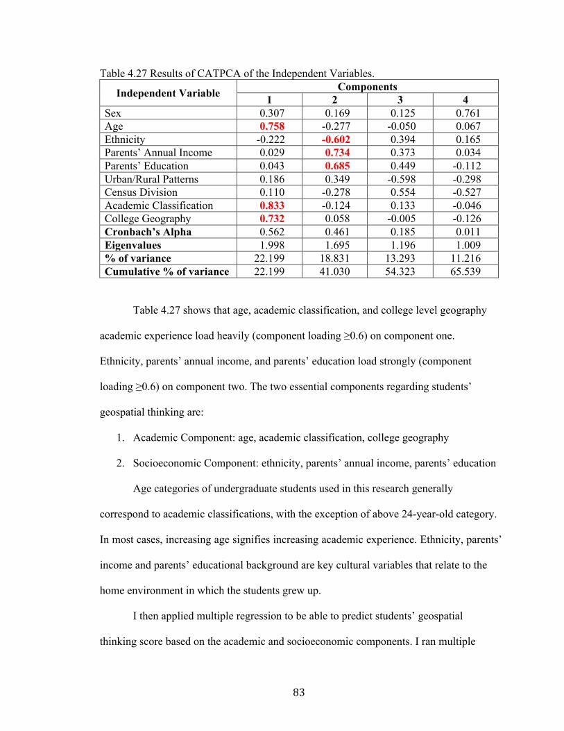
83

Table 4.27 Results of CATPCA of the Independent Variables.

Independent Variable Components 1 2 3 4

Sex 0.307 0.169 0.125 0.761 Age 0.758 -0.277 -0.050 0.067 Ethnicity -0.222 -0.602 0.394 0.165 Parents’ Annual Income 0.029 0.734 0.373 0.034 Parents’ Education 0.043 0.685 0.449 -0.112 Urban/Rural Patterns 0.186 0.349 -0.598 -0.298 Census Division 0.110 -0.278 0.554 -0.527 Academic Classification 0.833 -0.124 0.133 -0.046 College Geography 0.732 0.058 -0.005 -0.126 Cronbach’s Alpha 0.562 0.461 0.185 0.011 Eigenvalues 1.998 1.695 1.196 1.009 % of variance 22.199 18.831 13.293 11.216 Cumulative % of variance 22.199 41.030 54.323 65.539

Table 4.27 shows that age, academic classification, and college level geography

academic experience load heavily (component loading ≥0.6) on component one.

Ethnicity, parents’ annual income, and parents’ education load strongly (component

loading ≥0.6) on component two. The two essential components regarding students’

geospatial thinking are:

1. Academic Component: age, academic classification, college geography

2. Socioeconomic Component: ethnicity, parents’ annual income, parents’ education

Age categories of undergraduate students used in this research generally

correspond to academic classifications, with the exception of above 24-year-old category.

In most cases, increasing age signifies increasing academic experience. Ethnicity, parents’

income and parents’ educational background are key cultural variables that relate to the

home environment in which the students grew up.

I then applied multiple regression to be able to predict students’ geospatial

thinking score based on the academic and socioeconomic components. I ran multiple

84

regression with the object scores of the two components obtained by CATPCA. The

dependent variable was the geospatial thinking scores for 1479 students, and object

scores of academic and socioeconomic components for the 1479 students were

independent variables.

A significant model emerged using the backward method of multiple regression,

with F = 103.295, p <0.001, and adjusted R2 = 0.122 (Table 4.28). Although the model

explains only 12 percent of the total variance in the data, the model predicts robustly

within the 12 percent of variability. The regression model identified academic and

socioeconomic components as significant in predicting students’ geospatial thinking

(Table 4.29). Based on the values of standardized coefficients and the t statistic, academic

component is the stronger variable in predicting students’ geospatial thinking than the

socioeconomic component.

Table 4.28. Multiple Regression Model for Predicting Geospatial Thinking Scores. Dependent Variable Geospatial Thinking

Independent Variables Academic Component, Socioeconomic Component

Method, Model Backward, Model 1 R 0.350 R2 0.123 Adjusted R2 0.122 Standard Error of the Estimate 1.877

ANOVA F 103. 295 Sig. <0.001

Table 4.29. Coefficients of the Multiple Regression Model for Predicting Geospatial Thinking Scores.

Model 1

Unstandardized Coefficients

Standardized Coefficients t

Stat. Sig.

Value B Standard Error Beta

Constant 6.568 0.049 134.583 <0.001 Academic Component 0.580 0.049 0.290 11.880 <0.001 Socioeconomic Component 0.395 0.049 0.197 8.091 <0.001

85

Based on the unstandardized coefficients shown in Table 4.29, the regression

equation to predict students’ geospatial thinking score (GT Score) is:

GT Score = 6.568 + (0.580)(academic component) + (0.395)(socioeconomic component)

This regression equation can be used to predict students’ geospatial thinking score

(1-10 on GTS) for undergraduate students who have not taken the GTS. However, the

values of academic component and socioeconomic component are dependent on three

independent variables each: academic component (age, academic classification, and

college geography), and socioeconomic component (ethnicity, parents’ annual income,

and parents’ education). To predict the values of academic component and

socioeconomic component, I ran two more multiple regressions.

For the academic component multiple regression, I drew from the academic

component object scores produced by the foregoing CATPCA for the 1479 students as

the dependent variable, with age, academic classification, and college geography as

independent variables. The categories in these three independent variables are ordinal, so

I encoded the variables into eight dummy variables (18-20 year old; 21-24 years old;

freshman; sophomore; junior; no college geography courses; 1-2 college geography

courses; and 3-5 college geography courses). A strong model emerged using the

backward method of multiple regression, with F = 3417.477, p <0.001, and adjusted R2 =

0.949 (Table 4.30), accounting for 94 percent of the total variance in the data. Table 4.31

displays the coefficients of the regression model for the academic component.

86

Table 4.30. Multiple Regression Model for Predicting Academic Component Values. Dependent Variable Academic Component

Independent Variables Age Academic Classification College Geography


ANOVA F 3417.477 Sig. <0.001

Table 4.31. Coefficients of the Multiple Regression Model for Predicting Academic Component Values.

Model 1


Standardized Coefficients t

Stat. Sig.


Constant 1.968 0.019 101.445 <0.001 18-20 Years -1.007 0.019 -0.503 -52.078 <0.001 21-24 Years -0.510 0.018 -0.238 -28.441 <0.001 Freshman -1.180 0.024 -0.455 -48.630 <0.001 Sophomore -0.809 0.022 -0.349 -36.646 <0.001 Junior -0.417 0.018 -0.185 -23.388 <0.001 No College Geography -1.313 0.022 -0.494 -58.835 <0.001 1-2 College Geography -0.898 0.018 -0.447 -49.106 <0.001 3-5 College Geography -0.448 0.023 -0.139 -19.196 <0.001


equation to predict the academic component value is:

Academic Component = 1.968 + (-1.007)(18-20 age group) + (-0.510)(21-24 age group) + (-1.180)(freshman) + (-0.809)(sophomore) + (-0.417)(junior) + (-1.313)(no college geography course) + (-0.898)(1-2 college geography courses) + (-0.448)(3-5 college geography courses)

In the equation, the presence of a characteristic in student data equals 1, and the

absence of any characteristic equals 0. For example, if a student belongs to the age group

18-20, 1 is used in the equation, and the student does not automatically belong to the age

87

group 21-24, thus the value is 0. Similarly, if a student is senior, then all three values in

the equation for freshman, sophomore, and junior are 0.

For the socioeconomic component multiple regression, I incorporated the

socioeconomic component object scores produced by CATPCA for 1479 students as the

dependent variable, and ethnicity, parents’ annual income, and parents’ education became

the independent variables. The categories in these three independent variables are

nominal and ordinal, so I encoded these three variables into ten dummy variables: white,

Hispanic. Black, <$25,000, $25,000-$50,000, $51,000-$75,000, less than high school,

high school, associate degree, and bachelor degree. Once again, a strong model resulted

from the backward method of multiple regression, with F = 1121.995, p <0.001, and

adjusted R2 = 0.884 (Table 4.32), accounting for 88 percent of the total variance in the

data. Table 4.33 displays the coefficients for the socioeconomic component regression

model.

Table 4.32. Multiple Regression Model for Predicting Socioeconomic Component Values. Dependent Variable Socioeconomic Component

Independent Variables Ethnicity Parents’ Annual Income Parents’ Education


ANOVA F 1121.995 Sig. <0.001

88

Table 4.33. Coefficients of the Multiple Regression Model for Predicting Socioeconomic Component Values.

Model 1


Standardized Coefficients T

Stat. Sig.


Constant -0.142 0.038 -3.734 <0.001 Ethnicity: White 1.357 0.034 0.591 39.612 <0.001 Ethnicity: Hispanic 0.778 0.044 0.225 17.659 <0.001 Ethnicity: Black 0.431 0.044 0.121 9.700 <0.001 Parents’ Income: <$25K -1.279 0.030 -0.458 -43.305 <0.001 Parents’ Income: $25K-50K -0.821 0.025 -0.349 -32.834 <0.001 Parents’ Income: $51K-75K -0.366 0.024 -0.153 -15.217 <0.001 Parents’ Education: <HS -1.300 0.052 -0.258 -24.827 <0.001 Parents’ Education: HS -0.982 0.027 -0.436 -35.955 <0.001 Parents’ Education: AA -0.690 0.033 -0.219 -20.906 <0.001 Parents’ Education: BA/BS -0.325 0.024 -0.154 -13.394 <0.001


equation predicting the socioeconomic component value is:

Socioeconomic Component = -0.142 + (1.357)(white) + (0.778)(Hispanic) + (0.431)(black) + (-1.279)(parents’ income <$25,000) + (-0.821)(parents’ income $25,000-$50,000) + (-0.366)(parents’ income $51,000-$75,000) + (-1.300)(parents’ education less than high school) + (-0.982)(parents’ education high school) + (-0.690)(parents’ education associate degree) + (-0.325)(parents’ education bachelor degree)

In the equation and as with the academic component, the presence of a

characteristic for a student equals 1, and the absence of any characteristic equals 0. For

example, if a student is white, 1 is used in the equation in place of white, and the student

does not automatically belong to Hispanic or black category, so these values are 0.

Similarly, if parents’ annual income for a student is above $75,000, then all three values

in the equation for parents’ annual income of <$25,000, $25,000-$50,000, and $51,000-

$75,000 are 0.

89

In sum, the values of the academic and socioeconomic components for a student

can predict student’s geospatial thinking score using this equation:

GT Score = 6.568 + (0.580)(academic component) + (0.395)(socioeconomic component)

Geospatial Thinking Score Prediction: Data Mining Model

To predict the outcome of geospatial thinking of a student based on certain

independent variables, I also employed a data mining predictive model, which I call the

Geospatial Thinking Model (GTM). The Cubist software constructed the GTM. Cubist is

an artificial intelligence tool for generating rule-based predictive models (Cubist 2014).

Artificial intelligence includes expert system or a computer system that can simulate

human reasoning and decision-making ability. Cubist models predict numeric values, in

this case geospatial thinking scores. The elements of an expert system include:

1. Fact: an evidence (or value) of an attribute relevant to the phenomenon

(geospatial thinking score).

2. Rule: conditional statement(s) that relate a given circumstance to an outcome (e.g.,

a student’s score on the GTS is predicted based on sex, ethnicity, and academic

classification) (Chow 2012; Cubist 2014).

Cubist estimates a case's target value in terms of its attribute values by building a

model containing one or more rules, where each rule is a conjunction of conditions

associated with a linear expression. The meaning of a rule is that, if a case satisfies all the

conditions, then the linear expression is appropriate for predicting the target value. A

Cubist model thus resembles a piecewise linear model, except that the rules can overlap

(Cubist 2014).

90

Cubist employs heuristics that try to simplify models without substantially

reducing their predictive accuracy (Cubist 2014). However, Cubist includes different

methods for combining rule-based and instance-based models. After running several

iterations of model selections using different options, I chose only rule-based models as

recommended by the Cubist software based on the data analyzed by selecting the option:

Let Cubist Decide. This option derives from the training data a heuristic estimate of the

accuracy of each type of model and chooses the form that performs more accurately

(Cubist 2014). For model building, I first used geospatial thinking scores of 1479

students as the dependent variable, termed the target attribute in Cubist, and nine

independent variables (attributes): age, sex, ethnicity, parents’ annual income, parents’

education, urban/suburban/rural patterns, academic classification, academic major, and

college geography courses.

The first-run Cubist model produced five rules as shown in Table 4.34. Although

the order of the rules does not affect the value predicted by a model, Cubist presents them

in decreasing order of importance. The first rule makes the greatest contribution to the

model's accuracy on the training data, and the last rule has the least impact (Cubist 2014).

Thus, rule 1 in Table 4.34 is the most important, and rule 5 is the least. Expert systems,

like Cubist, select only the most important variables to generate rules that can predict

most cases. Ethnicity and academic major stand out as contributing variables in

predicting geospatial thinking of most cases.

Each rule also carries some descriptive information: the number of training cases

that satisfy the rule's conditions, their target values' mean, and a rough estimate of the

expected error magnitude of predictions made by the rule (Table 4.34).

91

Table 4.34. Cubist First-Run Model to Predict Students’ Geospatial Thinking Score (GT Score) Dependent Variable Geospatial Thinking

Independent Variables

Age, Sex, Ethnicity, Parents’ Annual Income, Parents’ Education, Urban/Suburban/Rural Patterns, Academic Classification, Academic Major, College Geography Courses

Number of Rules 5 (Option: Let Cubist Decide)

Number of Instances 7 nearest neighbors (Option: Let Cubist Decide)

Attribute Usage 100% Ethnicity, 100% Academic Major

Rule #

Training Cases Mean Estimated

Error Rule

1 179 4.9 1.9

If Ethnicity in Hispanic, Black Academic Major in Computer Science, Health, Nursing, Psychology, Criminal Justice, Social Science, Business, Education, Communication, Humanities, No Major then GT score = 5

2 219 5.8 1.6

If Ethnicity in White, Asian Academic Major in Criminal Justice, Education, Communication, No Major then GT score = 6

3 414 6.4 1.5

If Ethnicity in White, Asian Academic Major in Computer Science, Health, Nursing, Psychology, Social Science, Business, Humanities then GT score = 7

4 131 6.5 1.6

If Ethnicity in Hispanic, Black, Asian Academic Major in Geography, Geology, Environmental Science, Biology, Engineering, Science, History then GT score = 7

5 536 7.6 1.1

If Ethnicity in White Academic Major in Geography, Geology, Environmental Science, Biology, Engineering, Science, History then GT score = 8

Within the linear formula, the attributes are ordered in decreasing relevance to the

result (Cubist 2014). In each of the five rules, then, ethnicity is a stronger predictor of

geospatial thinking, followed by academic major. A comparative analysis of the first

three rules show white and Asian students have higher geospatial thinking scores than

92

Hispanic and black students across similar academic majors. Rules 4 and 5 clearly imply

that all ethnic groups are capable of increasing their geospatial thinking scores with

interventions by taking such courses as geography and geology, and science courses.

Even with a similar geospatial intervention, however, geospatial thinking scores of white

students are predicted to be higher than those of Hispanic, black, and Asian students.

Designing appropriate curricular geospatial materials to improve geospatial thinking of

Hispanic and black students in particular is critical.

Cubist models are evaluated on the training data from which they were generated.

The relative error magnitude is the ratio of the average error magnitude to the error

magnitude that would result from always predicting the mean value. Useful models

should have a relative error of magnitude less than 1 (Cubist 2014). The first-run model

(Table 4.34) had a relative error of 0.86, meaning the model is effective in geospatial

thinking score prediction. The correlation coefficient measures the agreement between

the cases' actual values of the target attribute and those values predicted by the model

(Cubist 2014). The correlation coefficient for the first-run model was 0.44, which implies

that the actual and predicted geospatial thinking scores are only moderately correlated.

To consider the effect of independent variable(s) other than academic major in

influencing students’ geospatial thinking, I ran Cubist again with a different set of

independent variables, excluding academic major and including census division (Table

4.35). In the second iteration, I included age, sex, ethnicity, parents’ annual income,

parents’ education, urban/suburban/rural patterns, academic classification, college

geography courses, and census division, and the Cubist model generated three rules in the

order of importance as shown. Ethnicity and college geography are conspicuous as prime

93

variables in predicting geospatial thinking of most cases in the second run. Rules 1 and 2

emphasize that the geospatial thinking scores of Hispanic and black students are lower

than those of white and Asian students who have taken the same number of college

geography courses. Rule 3 clearly highlights that higher number of college geography

courses improves geospatial thinking.

Table 4.35. Cubist Second-Run Model to Predict Students’ Geospatial Thinking Score (GT Score) Dependent Variable Geospatial Thinking

Independent Variables

Age, Sex, Ethnicity, Parents’ Annual Income, Parents’ Education, Urban/Suburban/Rural Patterns, Academic Classification, College Geography, Census Division

Number of Rules 3 (Option: Let Cubist Decide)

Number of Instances 6 nearest neighbors (Option: Let Cubist Decide)

Attribute Usage 100% College Geography, 83% Ethnicity

Rule # Cases Mean Estimated

Error Rule

1 242 5.2 1.9

If Ethnicity in Hispanic, Black College Geography in None, 1-2 courses, 3-5 courses then GT score = 5

2 984 6.6 1.5

If Ethnicity in White, Asian College Geography in None, 1-2 courses, 3-5 courses then GT score = 7

3 253 7.7 0.9 If College Geography in >5 courses then GT score = 8

The second-run model (Table 4.35) had a relative error of 0.88, meaning the

model is effective in geospatial thinking score prediction. The correlation coefficient for

the second-run model was 0.36, which implies that the actual and predicted geospatial

thinking scores are only moderately correlated.

Both regression and data mining models identified ethnicity and academic

variables as important in determining students’ geospatial thinking. Students can work to

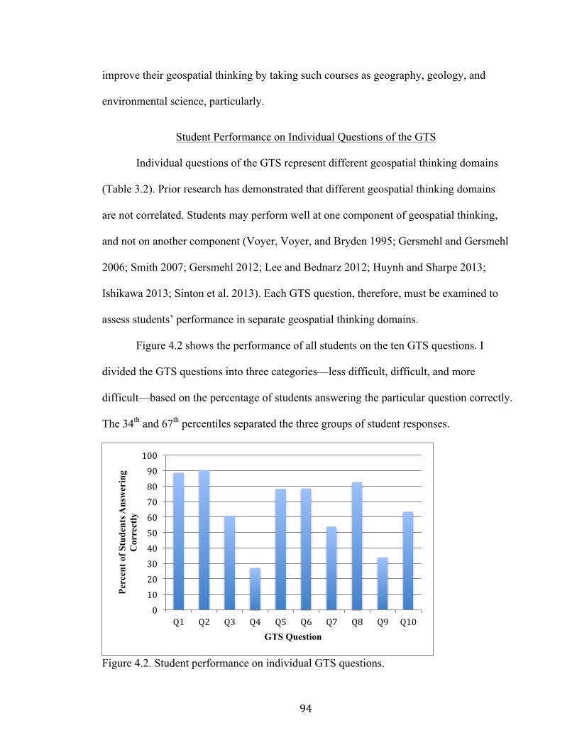
94

improve their geospatial thinking by taking such courses as geography, geology, and

environmental science, particularly.

Student Performance on Individual Questions of the GTS

Individual questions of the GTS represent different geospatial thinking domains

(Table 3.2). Prior research has demonstrated that different geospatial thinking domains

are not correlated. Students may perform well at one component of geospatial thinking,

and not on another component (Voyer, Voyer, and Bryden 1995; Gersmehl and Gersmehl

2006; Smith 2007; Gersmehl 2012; Lee and Bednarz 2012; Huynh and Sharpe 2013;

Ishikawa 2013; Sinton et al. 2013). Each GTS question, therefore, must be examined to

assess students’ performance in separate geospatial thinking domains.

Figure 4.2 shows the performance of all students on the ten GTS questions. I

divided the GTS questions into three categories—less difficult, difficult, and more

difficult—based on the percentage of students answering the particular question correctly.

The 34th and 67th percentiles separated the three groups of student responses.

Figure 4.2. Student performance on individual GTS questions.

0 10 20 30 40 50 60 70 80 90 100

Q1 Q2 Q3 Q4 Q5 Q6 Q7 Q8 Q9 Q10

Perc

ent o

f Stu

dent

s Ans

wer

ing

Cor

rect

ly

GTS Question

95

More than 67 percent students answered correctly questions 1 (geospatial pattern

and transition), 2 (direction and orientation), 5 (geospatial association), 6 (geospatial

shapes), and 8 (geospatial shapes). These questions were less difficult for a majority of

the students. If a question was answered correctly by 34-67 percent of students, then the

question was categorized as difficult question. Questions 3 (geospatial profile and

transition), 7 (geospatial shapes), and 10 (geospatial overlay) were difficult based on

students’ correct responses. If a question was answered correctly by less than 34 percent

of students, then the question was a more difficult question. Questions 4 (geospatial

association and transition) and 9 (geospatial shapes) were more difficult.

Table 4.36 depicts the difficulty level of GTS questions based on correct answers.

Interestingly, the four geospatial shapes questions included the three categories: less

difficult (Q8, Q6), difficult (Q7), and more difficult (Q9). This outcome can be linked to

the varying structures of the questions (see Appendix A). Within the geospatial shapes

domain, questions that were less difficult (Q8, Q6) involve analyzing points and lines

(networks) in terms of geographical data. The difficult question (Q7) requires the analysis

Table 4.36. Difficulty Level of GTS Questions Based on Students’ Responses (From Less Difficult to More Difficult).

Question Difficulty

Level

GTS Question Geospatial Thinking Domain

Percent of Students

Answering Correctly

Less Difficult

Q2 Direction and Orientation 90.3 Q1 Geospatial Pattern and Transition 88.6 Q8 Geospatial Shapes 82.6 Q6 Geospatial Shapes 78.4 Q5 Geospatial Association 78.1

Difficult Q10 Geospatial Overlay 63.4 Q3 Geospatial Profile and Transition 60.8 Q7 Geospatial Shapes 53.8

More Difficult Q9 Geospatial Shapes 33.9 Q4 Geospatial Association and Transition 27.0

96

of lines and areas (polygons and regions), and more difficult question (Q9) entails

analyzing points and areas. Within a single geospatial thinking domain, therefore,

students understand and analyze geospatial shapes differently.

Q5 from geospatial association and transition domain was less difficult, while Q4

from the same domain was more difficult (Table 4.36). Q5 requires students to search for

geospatial association (similar patterns) between two maps. Q4 compels students to first

discern geospatial association between two maps, and then transfer the information to a

graph. More complex geospatial reasoning processes make questions more difficult even

within similar geospatial domains.

Direction and orientation (Q2) was the easiest question on the GTS for most of

the students (Table 4.36). Undergraduate students seem to be good at map navigation,

way finding, and route planning. Geospatial pattern and transition (Q1) was also very

easy for students, underscoring that undergraduate students appear to be comfortable in

discerning geospatial patterns, transferring map information to graphic information, and

graphing geospatial transitions. Results for Q10 (geospatial overlay) suggest that students

are also fairly good at comprehending overlaying and dissolving map layers to choose the

best location based on various geographical conditions, connections, and distance.

Students find geospatial profile and transition difficult in comprehension than other

questions. Student understanding of geospatial shapes vary from being less difficult to

more difficult, depending on the number and level of concepts, and reasoning processes

involved in the analysis. Geospatial association with transition is difficult for

undergraduate students.

97

The analysis of difficulty level of GTS questions in Table 4.36 demonstrates that

students comprehend and apply geospatial thinking domains differently. The division of

spatial concepts and spatial reasoning processes into hierarchies (Golledge 1995; Jo and

Bednarz 2009) seem to be inconsequential, because responses from the GTS show

students answering questions from similar domains (similar conceptual and reasoning

levels) at the two ends of the range of difficulty. Both direction and shape are simple-

spatial concepts, according to Jo and Bednarz (2009), but students found the direction

question less difficult, and geospatial shapes questions at all three levels of difficulty.

Spatial association is a complex-spatial concept, according to Jo and Bednarz (2009), yet

student responses were at both ends of the difficulty range in different questions.

Although spatial pattern, profile, association, and overlay are higher-order complex-

spatial concepts (Jo and Bednarz 2009), students do not necessarily find them as more

difficult than lower-order simple-spatial concepts of direction and shape. Q3 requires

students to visualize topographic profile and orient themselves in situ, thereby entailing

higher order spatial reasoning process at the output level (Jo and Bednarz 2009). All

other questions on the GTS are at the processing level, which is the mid-level of spatial

reasoning, according to Jo and Bednarz (2009). However, students did not perceive Q3 to

be more difficult than other questions. The theoretical assumptions of the difficulty level

of questions based on spatial conceptual and reasoning hierarchy do not necessarily apply

to undergraduate students’ understanding and comprehension of different geospatial

thinking domains.

Different spatial and geospatial thinking domains are not correlated but

interconnected, as postulated by Gersmehl and Gersmehl (2006). Understanding group

98

and individual differences in students’ understanding of distinct geospatial thinking

domains is critical. An effective geography curriculum must comprehend student

strengths and weaknesses in various geospatial domains and then tailor teaching materials

to target improvement.

Group Differences on Individual Questions of the GTS

To substantiate statistically the foregoing generalizations regarding the difficulty

of individual GTS questions, I applied the chi-square test of independence (alpha = 0.05)

to investigate the relationships among the categories of each independent variable with

each GTS question, thereby inferring group differences. The chi-square test of

independence is a nonparametric method used to determine whether a significant

association exists between two categorical variables (Daniel 1990; Agresti 2002; Bearden

2014; Boduszek 2014). Each analysis of the chi-square test of independence included

each demographic, academic, or geographic variable as one variable, and each GTS

question as another variable. The students’ responses on individual questions were

categorical, as they were coded dichotomously, i.e. correct or incorrect. The six

independent variables—sex, age, ethnicity, academic classification, college geography,

and urban/suburban/rural patterns—were also categorical. To analyze whether a variable

and a particular GTS question were associated, I ran the chi-square test 60 times (six

independent variables by ten geospatial thinking questions). For example, one chi-square

run tested if understanding the geospatial thinking domain regarding geospatial overlay in

Q10 was independent of student ethnicity.

For Q1 representing geospatial pattern and transition domain, I ran a chi-square

for the six variables (Table 4.37). The understanding of geospatial pattern and transition

99

ability was independent of sex and age, yet the domain was associated with differences in

ethnicity, academic classification, college geography, and urban/suburban/rural locations.

Table 4.37. Association of Q1 (Geospatial Pattern and Transition) with Sex, Age, Ethnicity, Academic Classification, College Geography, and Urban/Suburban/Rural Patterns.

Variable Categories Number of Student

Responses (%) Chi-Square

p Value Result

Correct Incorrect

Sex Female 703 (87.4) 101 (12.6)

2.244 0.134

No difference exists in the responses of females and males to Q1

Male 607 (89.9) 68 (10.1)

Age 18-20 659 (87.7) 92 (12.3)

1.086 0.581

No differences exist in the responses of age groups to Q1

21-24 424 (89.6) 49 (10.4) >24 227 (89.0) 28 (11.0)

Ethnicity

White 1009 (91.5) 94 (8.5)

41.346 <0.01

Differences exist in the responses of ethnic groups to Q1

Hispanic 109 (80.1) 27 (19.9) Black 96 (75.6) 31 (24.4)

Asian 96 (85.0) 17 (15.0)


Freshman 233 (86.9) 35 (13.1)

9.461 0.024

Differences exist in the responses of academic classification groups to Q1

Sophomore 315 (86.1) 51 (13.9) Junior 352 (87.8) 49 (12.2)

Senior 410 (92.3) 34 (7.7)

College Geography Courses

No Geog. Course 206 (81.4) 47 (18.6)

40.589 <0.01

Differences exist in the responses of college geography groups to Q1

1-2 Geog. Courses 706 (86.9) 106 (13.1)

3-5 Geog. Courses 150 (93.2) 11 (6.8)

>5 Geog. Courses 248 (98.0) 5 (2.0)

Urban/ Suburban/ Rural

Urban 401 (84.4) 74 (15.6)

11.949 0.003

Differences exist in the responses of urban/sub-urban/rural groups to Q1

Suburban 575 (90.4) 61 (9.6)

Rural 334 (90.8) 34 (9.2)

100

Table 4.38 shows internal comparisons of significant associations between Q1

and different variables. The results suggest undergraduate curriculum needs to cater

specifically to Hispanic, black, and urban students, and students who have not taken any

college geography courses so their geospatial thinking ability in geospatial pattern and

transition can be strengthened. Senior students and students who have taken more than

five college geography courses have better understandings of geospatial pattern and

transition. Higher educational experience and formal college geography instruction are

keys in improving student comprehension of geospatial pattern and transition.

Table 4.38. Internal Comparisons for Association of Q1 (Geospatial Pattern and Transition) with Ethnicity, Academic Classification, College Geography, and Urban/Suburban/Rural Patterns.

Variable Categories Standardized Residuals Significant Contributors to the

Association and Internal Comparisons Correct Incorrect

Ethnicity

White 1.0 -2.9 Fewer white students than expected answered Q1 incorrectly, thus outperforming the other ethnic groups. More Hispanic and black students than expected answered Q1 incorrectly, thus underperforming the other ethnic groups.

Hispanic -1.0 2.9

Black -1.6 4.3

Asian -0.4 1.1


Freshman -0.3 0.8 Fewer senior students than expected answered Q1 incorrectly, thus outperforming the other academic classification groups.

Sophomore -0.5 1.4 Junior -0.2 0.5 Senior 0.8 -2.3


No Geog. Course -1.2 3.4 More students with no college

geography than expected answered Q1 incorrectly, thus under-performing the other groups. Fewer students with >5 college geography courses than expected answered Q1 incorrectly, thus outperforming the other groups.

1-2 Geog. Courses -0.5 1.4

3-5 Geog. Courses 0.6 -1.7

>5 Geog. Courses 1.6 -4.4


Urban -1.0 2.7 More urban students than expected answered Q1 incorrectly, thus underperforming the other groups.

Suburban 0.5 -1.4 Rural 0.4 -1.2

101

The geospatial thinking ability to comprehend direction and orientation (Q2) was

related to differences in ethnicity and urban/suburban/rural locations (Table 4.39).

Table 4.39. Association of Q2 (Direction and Orientation) with Sex, Age, Ethnicity, Academic Classification, College Geography, and Urban/Suburban/Rural Patterns.



p Value Result

Correct Incorrect

Sex Female 718 (89.3) 86 (10.7)

1.848 0.174


Male 617 (91.4) 58 (8.6)

Age

18-20 668 (88.9) 83 (11.1)

3.481 0.175


21-24 436 (92.2) 37 (7.8)

>24 231 (90.6) 24 (9.4)

Ethnicity

White 1014 (91.9) 89 (8.1)

16.775 0.001


Hispanic 120 (88.2) 16 (11.8) Black 104 (81.9) 23 (18.1) Asian 97 (85.8) 16 (14.2)


Freshman 237 (88.4) 31 (11.6)

4.872 0.181

No differences exist in the responses of academic classification groups to Q2

Sophomore 328 (89.6) 38 (10.4)

Junior 358 (89.3) 43 (10.7) Senior 412 (92.8) 32 (7.2)


No Geog. Course 220 (87.0) 33 (13.0)

7.673 0.053

No differences exist in the responses of college geography groups to Q2

1-2 Geog. Courses 729 (89.8) 83 (10.2)

3-5 Geog. Courses 149 (92.5) 12 (7.5)

>5 Geog. Courses 237 (93.7) 16 (6.3)


Urban 412 (86.7) 63 (13.3)

12.790 0.002

Differences exist in the responses of urban, suburban, rural groups to Q2

Suburban 577 (90.7) 59 (9.3)

Rural 346 (94.0) 22 (6.0)

Table 4.40 shows the internal comparisons of Q2 with ethnicity and

urban/suburban/rural locations. Black and urban students need geospatial instruction that

102

emphasizes direction and orientation skills. Rural students, when navigating, are

apparently more attuned to direction and orientation than urban students.

Table 4.40. Internal Comparisons for Association of Q2 (Direction and Orientation) with Ethnicity, and Urban/Suburban/Rural Patterns.

Variable Categories Standardized Residuals Significant Contributors to the Association and Internal

Comparisons Correct Incorrect

Ethnicity

White 0.6 -1.8 More black students than expected answered Q2 incorrectly, thus underperforming the other ethnic groups.

Hispanic -0.2 0.8 Black -1.0 3.0 Asian -0.5 1.5


Urban -0.8 2.5 More urban students than expected answered Q2 incorrectly, thus underperforming the other groups. Fewer rural students than expected answered Q2 incorrectly, thus outperforming the other groups.

Suburban 0.1 -0.4

Rural 0.8 -2.3

Q3, geospatial profile and transition, is related to differences in sex, age, ethnicity,

academic classification, college geography, and urban/suburban/rural locations (Table

4.41). In the geospatial profile and transition domain, students who were female,

Hispanic, black, urban, younger, freshman, and less exposed to formal geography courses

underperformed more than expected (Table 4.42). These groups of students may require

additional classroom instruction in geospatial profile and transition thinking ability.

103

Table 4.41. Association of Q3 (Geospatial Profile and Transition) with Sex, Age, Ethnicity, Academic Classification, College Geography, and Urban/Suburban/Rural Patterns.



p Value Result

Correct Incorrect

Sex Female 427 (53.1) 377 (46.9)

43.532 <0.01

Difference exists in the responses of females and males to Q3 Male 472 (69.9) 203 (30.1)

Age

18-20 417 (55.5) 334 (44.5)

20.316 <0.01

Differences exist in the responses of age groups to Q3

21-24 303 (64.1) 170 (35.9)

>24 179 (70.2) 76 (29.8)

Ethnicity

White 731 (66.3) 372 (33.7)

69.968 <0.01




Freshman 136 (50.7) 132 (49.3)

25.823 <0.01


Sophomore 219 (59.8) 147 (40.2) Junior 236 (58.9) 165 (41.1) Senior 308 (69.4) 136 (30.6)


No Geog. Course 134 (53.0) 119 (47.0)

68.577 <0.01


1-2 Geog. Courses 450 (55.4) 362 (44.6)

3-5 Geog. Courses 106 (65.8) 55 (34.2)

>5 Geog. Courses 209 (82.6) 44 (17.4)


Urban 256 (53.9) 219 (46.1)

13.965 0.001

Differences exist in the responses of urban, sub-urban, rural groups to Q3

Suburban 406 (63.8) 230 (36.2)

Rural 237 (64.4) 131 (35.6)

104

Table 4.42. Internal Comparisons for Association of Q3 (Geospatial Profile and Transition) with Sex, Age, Ethnicity, Academic Classification, College Geography, and Urban/ Suburban/Rural Patterns.

Variable Categories Standardized

Residuals Significant Contributors to the


Sex

Female -2.8 3.5

Fewer female students than expected answered Q3 correctly, and more female students than expected answered Q3 incorrectly. More male students than expected answered Q3 correctly, and fewer male students than expected answered Q3 incorrectly. Thus, males outperformed females.

Male 3.0 -3.8

Age

18-20 -1.8 2.3 More 18-20 year old students than expected answered Q3 incorrectly, thus underperforming the other age groups. Fewer >24-year-old students than expected answered Q3 incorrectly, thus outperforming the other age groups.

21-24 0.9 -1.1

>24 1.9 -2.4

Ethnicity

White 2.3 -2.9 More white students than expected answered Q3 correctly, and fewer white students than expected answered Q3 incorrectly. Thus, whites outperformed the other ethnic groups. Fewer Hispanic and black students than expected answered Q3 correctly, and more Hispanic and black students than expected answered Q3 incorrectly. Thus, Hispanics and blacks underperformed the other ethnic groups.

Hispanic -2.2 2.7

Black -4.1 5.1

Asian -0.6 0.7


Freshman -2.1 2.6 Fewer freshmen than expected answered Q3 correctly, and more freshmen than expected answered Q3 incorrectly. Thus, freshmen underperformed the other groups. More senior students than expected answered Q3 correctly, and fewer seniors than expected answered Q3 incorrectly. Thus, seniors outperformed the other groups.

Sophomore -0.2 0.3

Junior -0.5 0.6

Senior 2.3 -2.9


No Geography Course

-1.6 2.0 More students with no college geography courses than expected answered Q3 incorrectly, thus underperforming the other groups. Fewer students with 1-2 college geography courses than expected answered Q3 correctly, and more students with 1-2 college geography


-2.0 2.4

105

Table 4.42. Continued.





3-5 Geography Courses 0.8 -1.0

courses than expected answered Q3 incorrectly, thus underperforming the other groups. More students with >5 college geography courses than expected answered Q3 correctly, and fewer students with >5 college geography courses than expected answered Q3 incorrectly, thus outperforming the other groups.

>5 Geography Courses 4.5 -5.5

Urban/Sub-urban/Rural



Q4, geospatial association and transition, was related to differences in age, and

academic classification (Table 4.43), and Table 4.44 displays internal comparisons of

significant associations of Q4. In the geospatial association and transition domain,

students above 24 years of age underperformed more than expected. Geospatial

association and transition was the most difficult geospatial domain according to the

performance of students on the GTS. Only 27 percent were able to answer Q4 correctly

(Table 4.33). Students need more practice in geospatial association and transition

geospatial thinking.

106

Table 4.43. Association of Q4 (Geospatial Association and Transition) with Sex, Age, Ethnicity, Academic Classification, College Geography, and Urban/Suburban/Rural Patterns.



p Value Result

Correct Incorrect

Sex Female 213 (26.5) 591 (73.5)

0.273 0.601


Male 187 (27.7) 488 (72.3)

Age

18-20 218 (29.0) 533 (71.0)

17.511 <0.01


21-24 140 (29.6) 333 (70.4)

>24 42 (16.5) 213 (83.5)

Ethnicity

White 305 (27.7) 798 (72.3)

5.698 0.127

No differences exist in the responses of ethnic groups to Q4



Freshman 76 (28.4) 192 (71.6)

9.178 0.027


Sophomore 87 (23.8) 279 (76.2) Junior 96 (23.9) 305 (76.1)

Senior 141 (31.8) 303 (68.2)


No Geog. Course 69 (27.3) 184 (72.7)

2.049 0.562


1-2 Geog. Courses 209 (25.7) 603 (74.3)

3-5 Geog. Courses 46 (28.6) 115 (71.4)

>5 Geog. Courses 76 (30.0) 177 (70.0)


Urban 119 (25.1) 356 (74.9)

1.603 0.449

No differences exist in the responses of urban, sub-urban, rural groups to Q4

Suburban 181 (28.5) 455 (71.5)

Rural 100 (27.2) 268 (72.8)

107

Table 4.44. Internal Comparisons for Association of Q4 (Geospatial Association and Transition) with Age, and Academic Classification.




Age

18-20 1.0 -0.6 Fewer >24 year old students than expected answered Q4 correctly, and more >24 year old students than expected answered Q4 incorrectly, thus underperforming the other age groups.

21-24 1.1 -0.7

>24 -3.2 2.0


Freshman 0.4 -0.3

None Sophomore -1.2 0.7 Junior -1.2 0.7 Senior 1.9 -1.2

Q5, geospatial association, was related to differences in sex, age, ethnicity,


4.45). Hispanic, black, and urban students and students who had taken no college

geography courses underperformed more than expected (Table 4.46), consequently

pointing to more classroom instruction and practice in geospatial association. Male,

senior, and rural students and students who had taken more than five college geography

courses performed better than expected.

108

Table 4.45. Association of Q5 (Geospatial Association) with Sex, Age, Ethnicity, Academic Classification, College Geography, and Urban/Suburban/Rural Patterns.



p Value Result

Correct Incorrect

Sex Female 610 (75.9) 194 (24.1)

5.087 0.024


Age 18-20 562 (74.8) 189 (25.2)

9.480 0.009 Differences exist in the responses of age groups to Q5

21-24 385 (81.4) 88 (18.6) >24 208 (81.6) 47 (18.4)

Ethnicity

White 918 (83.2) 185 (16.8)

76.159 <0.01




Freshman 196 (73.1) 72 (26.9)

13.475 0.004




No Geog. Course 177 (70.0) 76 (30.0)

31.310 <0.01


1-2 Geog. Courses 620 (76.4) 192 (23.6)

3-5 Geog. Courses 132 (82.0) 29 (18.0)

>5 Geog. Courses 226 (89.3) 27 (10.7)


Urban 344 (72.4) 131 (27.6)

15.076 0.001

Differences exist in the responses of urban, suburban, rural groups to Q5

Suburban 505 (79.4) 131 (20.6)

Rural 306 (83.2) 62 (16.8)

109

Table 4.46. Internal Comparisons for Association of Q5 (Geospatial Association) with Sex, Age, Ethnicity, Academic Classification, College Geography, and Urban/Suburban/Rural Patterns.




Sex Female -0.7 1.3 None Male 0.8 -1.5

Age 18-20 -1.0 1.9

None 21-24 0.8 -1.5 >24 0.6 -1.2

Ethnicity

White 1.9 -3.6 Fewer Hispanic and black students than expected answered Q5 correctly, and more Hispanic and black students than expected answered Q5 incorrectly. Thus, Hispanics and blacks underperformed the other ethnic groups.

Hispanic -2.3 4.3

Black -2.7 5.2

Asian -0.7 1.3


Freshman -0.9 1.7 Fewer seniors than expected answered Q5 incorrectly, thus outperforming the other groups.

Sophomore -0.6 1.2 Junior 0.0 0.0 Senior 1.3 -2.5


No Geog. Course -1.5 2.8

More students with no college geography course than expected answered Q5 incorrectly, thus underperforming the other groups. More students with >5 college geography courses than expected answered Q5 correctly, and fewer students with >5 college geography courses than expected answered Q5 incorrectly, thus outperforming the other groups.





Urban -1.4 2.6 More urban students than expected answered Q5 incorrectly, thus underperforming the other groups. Fewer rural students than expected answered Q5 incorrectly, thus outperforming the other groups.

Suburban 0.4 -0.7

Rural 1.1 -2.1

Q6, geospatial shapes, was related to differences in sex, age, ethnicity, academic

classification, college geography, and urban/suburban/rural locations (Table 4.47).

Female, younger (18-20 years old), Hispanic, black, Asian, freshman, and urban students,

and students with no or 1-2 college geography courses underperformed more than

expected (Table 4.48). These groups of students may require supplementary classroom

110

instruction and practice in comprehending geospatial shapes. Male, older (above 24 years

old), white, senior, and rural students and students who had taken more than five college

geography courses performed better than expected.

Table 4.47. Association of Q6 (Geospatial Shapes) with Sex, Age, Ethnicity, Academic Classification, College Geography, and Urban/Suburban/Rural Patterns.



p Value Result

Correct Incorrect

Sex Female 609 (75.7) 195 (24.3)

7.119 0.008


Age

18-20 556 (74.0) 195 (26.0)

19.022 <0.01


21-24 384 (81.2) 89 (18.8)

>24 219 (85.9) 36 (14.1)

Ethnicity

White 938 (85.0) 165 (15.0)

129.13 <0.01




Freshman 189 (70.5) 79 (29.5)

27.867 <0.01




No Geog. Course 178 (70.4) 75 (29.6)

67.152 <0.01


1-2 Geog. Courses 603 (74.3) 209 (25.7)

3-5 Geog. Courses 135 (83.9) 26 (16.1)

>5 Geog. Courses 243 (96.0) 10 (4.0)


Urban 332 (69.9) 143 (30.1)

32.593 <0.01


Suburban 513 (80.7) 123 (19.3)

Rural 314 (85.3) 54 (14.7)

111

Table 4.48. Internal Comparisons for Association of Q6 (Geospatial Shapes) with Sex, Age, Ethnicity, Academic Classification, College Geography, and Urban/Suburban/Rural Patterns.





Age

18-20 -1.3 2.6 More 18-20-year-old students than expected answered Q6 incorrectly, thus underperforming the other age groups. Fewer >24 year old students than expected answered Q6 incorrectly, thus outperforming the other age groups.

21-24 0.7 -1.3

>24 1.4 -2.6

Ethnicity

White 2.5 -4.8 More white students than expected answered Q6 correctly, and fewer white students than expected answered Q6 incorrectly. Thus, whites outperformed the other ethnic groups. More Hispanic, black, and Asian students than expected answered Q6 incorrectly. Thus, Hispanics, blacks, and Asians underperformed the other ethnic groups. Fewer black students than expected answered Q6 correctly, thus underperforming the other groups.

Hispanic -1.8 3.4

Black -4.0 7.5

Asian -1.7 3.1


Freshman -1.5 2.8 More freshmen than expected answered Q6 incorrectly, thus underperforming the other groups. Fewer seniors than expected answered Q6 incorrectly, thus outperforming the other groups.




More students with no and 1-2 college geography courses than expected answered Q6 incorrectly, thus underperforming the other groups. More students with >5 college geography courses than expected answered Q6 correctly, and fewer students with >5 college courses experience than expected answered Q6 incorrectly, thus outperforming the other groups.





Urban -2.1 4.0 Fewer urban students than expected answered Q6 correctly, and more urban students than expected answered Q6 incorrectly, thus underperforming the other groups. Fewer rural students than expected answered Q6 incorrectly, thus outperforming the other groups.

Suburban 0.7 -1.2

Rural 1.5 -2.9

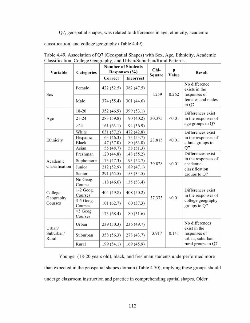
112

Q7, geospatial shapes, was related to differences in age, ethnicity, academic

classification, and college geography (Table 4.49).


Variable Categories Number of Students


p Value Result

Correct Incorrect

Sex Female 422 (52.5) 382 (47.5)

1.259 0.262


Male 374 (55.4) 301 (44.6)

Age

18-20 352 (46.9) 399 (53.1)

30.375 <0.01 Differences exist in the responses of age groups to Q7

21-24 283 (59.8) 190 (40.2)

>24 161 (63.1) 94 (36.9)

Ethnicity

White 631 (57.2) 472 (42.8)

23.815 <0.01




Freshman 120 (44.8) 148 (55.2)

39.828 <0.01




No Geog. Course 118 (46.6) 135 (53.4)

37.373 <0.01


1-2 Geog. Courses 404 (49.8) 408 (50.2)

3-5 Geog. Courses 101 (62.7) 60 (37.3)

>5 Geog. Courses 173 (68.4) 80 (31.6)


Urban 239 (50.3) 236 (49.7)

3.917 0.141

No differences exist in the responses of urban, suburban, rural groups to Q7

Suburban 358 (56.3) 278 (43.7)

Rural 199 (54.1) 169 (45.9)

Younger (18-20 years old), black, and freshman students underperformed more

than expected in the geospatial shapes domain (Table 4.50), implying these groups should

undergo classroom instruction and practice in comprehending spatial shapes. Older

113

(above 24 years old) and senior students, and students who had taken more than five

college geography classes performed better than expected.

Table 4.50. Internal Comparisons for Association of Q7 (Geospatial Shapes) with Age, Ethnicity, Academic Classification, and College Geography.


Residuals Significant Contributors to the Association

Correct Incorrect

Age

18-20 -2.6 2.8 Fewer 18-20-year-old students than expected answered Q7 correctly, and more 18-20-year-old students than expected answered Q7 incorrectly, thus underperforming the other age groups. More >24 year old students than expected answered Q7 correctly, and fewer >24-year-old students than expected answered Q7 incorrectly, thus outperforming the other age groups.

21-24 1.8 -1.9

>24 2.0 -2.2

Ethnicity

White 1.5 -1.7 Fewer black students than expected answered Q7 correctly, and more black students than expected answered Q7 incorrectly, thus underperforming the other ethnic groups.

Hispanic -1.2 1.3 Black -2.6 2.8 Asian -0.7 0.8


Freshman -2.0 2.2 Fewer freshmen than expected answered Q7 correctly, and more freshmen than expected answered Q7 incorrectly, thus underperforming the other groups. More seniors than expected answered Q7 correctly, and fewer seniors than expected answered Q7 incorrectly, thus outperforming the other groups.

Sophomore -1.7 1.8

Junior -0.3 0.3

Senior 3.4 -3.6


No Geog. Course -1.6 1.7 More students with >5 college

geography courses than expected answered Q7 correctly, and fewer students with >5 college geography courses than expected answered Q7 incorrectly, thus outperforming the other groups.




Q8, geospatial shapes, was related to differences in sex, age, ethnicity, academic

classification, college geography, and urban/suburban/rural locations (Table 4.51).

Younger (18-20 years old), black, and rural students, and students who had taken one to

114

two college geography courses underperformed more than expected (Table 4.52), perhaps

needing additional classroom instruction and practice in comprehending geospatial

shapes. White, 21-24-year-old, and senior students, and students who had taken 3-5 or

more than five college geography courses performed better than expected.




p Value Result

Correct Incorrect

Sex Female 646 (80.3) 158 (19.7)

5.961 0.015


Age 18-20 591 (78.7) 160 (21.3)

16.091 <0.01


21-24 412 (87.1) 61 (12.9) >24 218 (85.5) 37 (14.5)

Ethnicity

White 949 (86.0) 154 (14.0)

65.883 <0.01




Freshman 209 (78.0) 59 (22.0)

24.000 <0.01




No Geog. Course 205 (81.0) 48 (19.0)

54.929 <0.01


1-2 Geog. Courses 628 (77.3) 184 (22.7)

3-5 Geog. Courses 144 (89.4) 17 (10.6)

>5 Geog. Courses 244 (96.4) 9 (3.6)


Urban 373 (78.5) 102 (21.5)

7.909 0.019


Suburban 538 (84.6) 98 (15.4)

Rural 310 (84.2) 58 (15.8)

115

Table 4.52. Internal Comparisons for Association of Q8 (Geospatial Shapes) with Sex, Age, Ethnicity, Academic Classification, College Geography, and Urban/Suburban/Rural Patterns.





Age

18-20 -1.2 2.5 More 18-20-year-old students than expected answered Q8 incorrectly, thus underperforming the other age groups. Fewer 21-24-year-old students than expected answered Q8 incorrectly, thus outperforming the other age groups.

21-24 1.1 -2.4

>24 0.5 -1.1

Ethnicity

White 1.3 -2.8 Fewer white students than expected answered Q8 incorrectly, thus outperforming the other ethnic groups. Fewer black students than expected answered Q8 correctly, and more black students than expected answered Q8 incorrectly, thus underperforming the other ethnic groups.

Hispanic -0.9 1.9

Black -3.0 6.6

Asian 0.2 -0.4


Freshman -0.8 1.8 Fewer seniors than expected answered Q8 incorrectly, thus outperforming the other groups.




More students with 1-2 college geography courses than expected answered Q8 incorrectly, thus underperforming the other groups. Fewer students with 3-5 college geography courses than expected answered Q8 incorrectly, thus outperforming the other groups. More students with >5 college geography courses than expected answered Q8 correctly, and fewer students with >5 college courses than expected answered Q8 incorrectly, thus outperforming the other groups.







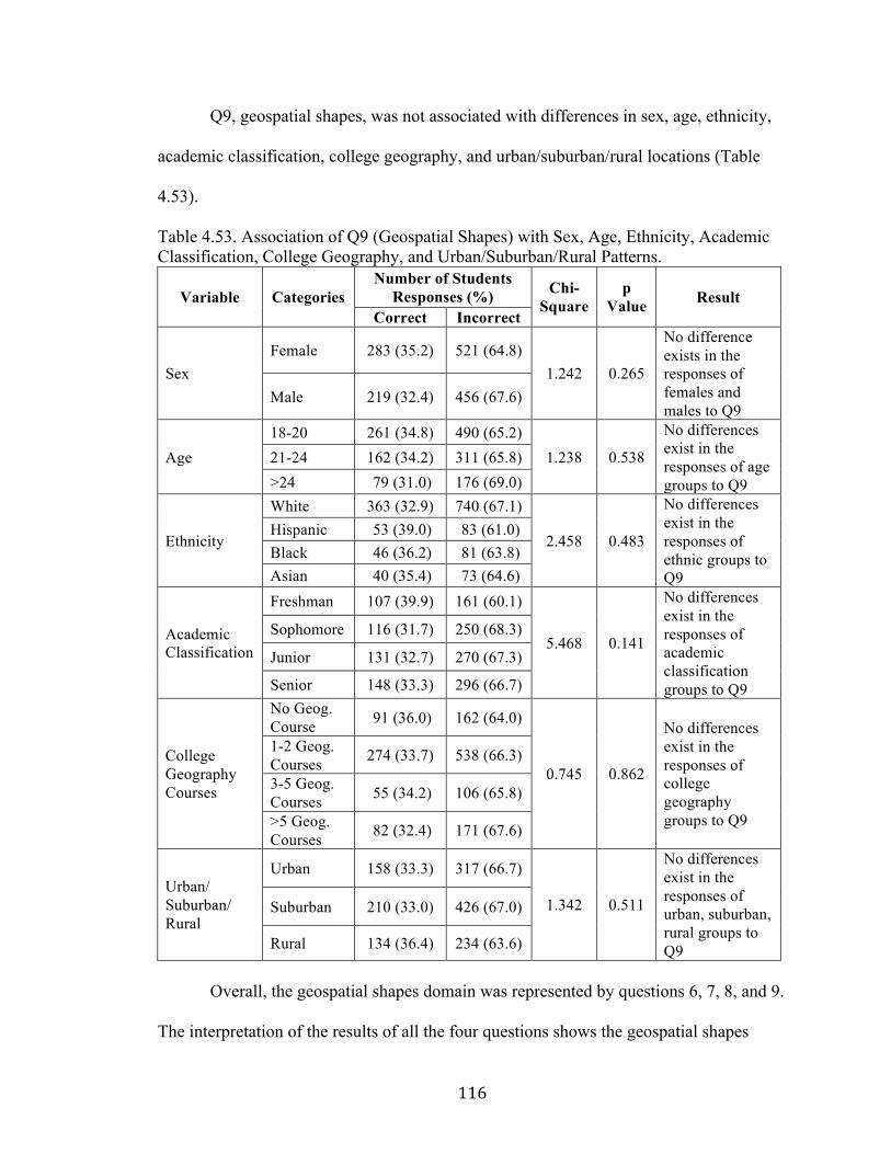
116

Q9, geospatial shapes, was not associated with differences in sex, age, ethnicity,


4.53).


Variable Categories Number of Students


p Value Result

Correct Incorrect

Sex Female 283 (35.2) 521 (64.8)

1.242 0.265


Male 219 (32.4) 456 (67.6)

Age 18-20 261 (34.8) 490 (65.2)

1.238 0.538


21-24 162 (34.2) 311 (65.8) >24 79 (31.0) 176 (69.0)

Ethnicity

White 363 (32.9) 740 (67.1)

2.458 0.483

No differences exist in the responses of ethnic groups to Q9



Freshman 107 (39.9) 161 (60.1)

5.468 0.141

No differences exist in the responses of academic classification groups to Q9

Sophomore 116 (31.7) 250 (68.3)

Junior 131 (32.7) 270 (67.3)

Senior 148 (33.3) 296 (66.7)


No Geog. Course 91 (36.0) 162 (64.0)

0.745 0.862


1-2 Geog. Courses 274 (33.7) 538 (66.3)

3-5 Geog. Courses 55 (34.2) 106 (65.8)

>5 Geog. Courses 82 (32.4) 171 (67.6)


Urban 158 (33.3) 317 (66.7)

1.342 0.511


Suburban 210 (33.0) 426 (67.0)

Rural 134 (36.4) 234 (63.6)

Overall, the geospatial shapes domain was represented by questions 6, 7, 8, and 9.

The interpretation of the results of all the four questions shows the geospatial shapes

117

domain was associated with sex, age, ethnicity, academic classification, college

geography, and urban/suburban/rural locations. Male, older (21-24 and above 24 years

old), white, senior, and rural students, and students who had taken 3-5 or more than five

college geography courses performed better than expected. These groups of students,

therefore, better understand geospatial shapes. Female, younger (18-20 years old),

Hispanic, black, Asian, freshman, and urban students, and students who had taken no or

only 1-2 college geography courses underperformed, thus implying the need for

intervention to improve their geospatial shapes skills.

Q10, geospatial overlay, was related to differences in sex, age, ethnicity,

academic classification, and college geography (Table 4.54). Female, younger (18-20

years old), black, and sophomore students, and students who had taken only 1-2 college

geography courses underperformed than expected (Table 4.55), indicating the students

should have more instruction and practice in comprehending geospatial overlay. Male,

white, older (above 24 years old), and senior students, and students who had taken more

than five college geography courses performed better than expected.

118

Table 4.54. Association of Q10 (Geospatial Overlay) with Sex, Age, Ethnicity, Academic Classification, College Geography, and Urban/Suburban/Rural Patterns.



p Value Result

Correct Incorrect

Sex Female 462 (57.5) 342 (42.5)

26.332 <0.01


Age 18-20 433 (57.7) 318 (42.3)

23.191 <0.01


21-24 319 (67.4) 154 (32.6) >24 185 (72.5) 70 (27.5)

Ethnicity

White 740 (67.1) 363 (32.9)

37.922 <0.01




Freshman 156 (58.2) 112 (41.8)

33.113 <0.01




No Geog. Course 145 (57.3) 108 (42.7)

70.070 <0.01


1-2 Geog. Courses 467 (57.5) 345 (42.5)

3-5 Geog. Courses 109 (67.7) 52 (32.3)

>5 Geog. Courses 216 (85.4) 37 (14.6)


Urban 285 (60.0) 190 (40.0)

4.290 0.117


Suburban 420 (66.0) 216 (34.0)

Rural 232 (63.0) 136 (37.0)

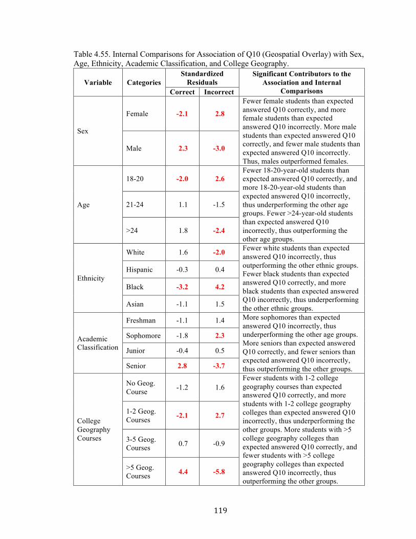
119

Table 4.55. Internal Comparisons for Association of Q10 (Geospatial Overlay) with Sex, Age, Ethnicity, Academic Classification, and College Geography.




Sex

Female -2.1 2.8

Fewer female students than expected answered Q10 correctly, and more female students than expected answered Q10 incorrectly. More male students than expected answered Q10 correctly, and fewer male students than expected answered Q10 incorrectly. Thus, males outperformed females.

Male 2.3 -3.0

Age

18-20 -2.0 2.6 Fewer 18-20-year-old students than expected answered Q10 correctly, and more 18-20-year-old students than expected answered Q10 incorrectly, thus underperforming the other age groups. Fewer >24-year-old students than expected answered Q10 incorrectly, thus outperforming the other age groups.

21-24 1.1 -1.5

>24 1.8 -2.4

Ethnicity

White 1.6 -2.0 Fewer white students than expected answered Q10 incorrectly, thus outperforming the other ethnic groups. Fewer black students than expected answered Q10 correctly, and more black students than expected answered Q10 incorrectly, thus underperforming the other ethnic groups.

Hispanic -0.3 0.4

Black -3.2 4.2

Asian -1.1 1.5


Freshman -1.1 1.4 More sophomores than expected answered Q10 incorrectly, thus underperforming the other age groups. More seniors than expected answered Q10 correctly, and fewer seniors than expected answered Q10 incorrectly, thus outperforming the other groups.

Sophomore -1.8 2.3

Junior -0.4 0.5

Senior 2.8 -3.7



Fewer students with 1-2 college geography courses than expected answered Q10 correctly, and more students with 1-2 college geography colleges than expected answered Q10 incorrectly, thus underperforming the other groups. More students with >5 college geography colleges than expected answered Q10 correctly, and fewer students with >5 college geography colleges than expected answered Q10 incorrectly, thus outperforming the other groups.




120

Table 4.56 summarizes the statistically significant associations of geospatial

thinking domains with six independent variables and displays outperforming and

underperforming groups of students in different domains. The main groups of students

that seem to need additional classroom instruction and training in various geospatial

thinking domains include females, younger students (18-20 years old), Hispanics, blacks,

freshmen, urban students, and students who had taken no or only 1-2 college geography

courses.

Table 4.56. Summary of Relationship of Geospatial Thinking Domains with Significant Variables.

GTS Question (Geospatial Thinking

Domain)

Significant Variables

Outperforming Groups

Underperforming Groups

Q1 (Geospatial Pattern and Transition)

Ethnicity White Hispanic and Black Academic Classification Senior

College Geography >5 College Geog. Courses

No College Geog. Course

Urban/Suburban/ Rural Patterns Urban

Q2 (Direction and Orientation)

Ethnicity Black Urban/Suburban/ Rural Patterns Rural Urban

Q3 (Geospatial Profile and Transition)

Sex Male Female Age >24 18-20 Ethnicity White Hispanic and Black Academic Classification Senior Freshman


No and 1-2 College Geog. Courses


Q4 (Geospatial Association and Transition)

Age >24

Q5 (Geospatial Association)

Ethnicity Hispanic and Black Academic Classification Senior


No College Geog. Course

Urban/Suburban/ Rural Patterns Rural Urban

121

Table 4.56. Continued. GTS Question

(Geospatial Thinking Domain)

Significant Variables

Outperforming Groups

Underperforming Groups

Q6 (Geospatial Shapes)

Age >24 18-20

Ethnicity White Hispanic, Black, and Asian

Academic Classification Senior Freshman


No and 1-2 College Geog. Courses

Urban/Suburban/ Rural Patterns Rural Urban


Age >24 18-20 Ethnicity Black Academic Classification Senior Freshman



Age 21-24 18-20 Ethnicity White Black Academic Classification Senior

College Geography >5 and 3-5 College Geog. Courses

1-2 College Geog. Courses


Q10 (Geospatial Overlay)

Sex Male Female Age >24 18-20 Ethnicity White Black Academic Classification Senior Sophomore


1-2 College Geog. Courses

Visualization of Responses for Individual GTS Questions

Visually corroborating the tabular chi-square results are six two-dimensional

diagrams displaying the results of statistically significant variables. Figure 4.3 shows

males performed better than females on most geospatial thinking questions. Males

performed significantly better than females in such geospatial thinking domains as

122

geospatial profiles and transition, geospatial association, geospatial shapes, and

geospatial overlay.

Figure 4.3. Student performance on GTS questions based on sex.

Figure 4.4 underscores that older students (above 24 years old) outperformed

younger students (18-20 years old) on most geospatial thinking questions. Older students

demonstrated a superior understanding of geospatial profile and transition, geospatial

shapes, and geospatial overlay, while younger students underperformed in these domains.

0

10

20

30

40

50

60

70

80

90

100

Q1 Q2 Q3 Q4 Q5 Q6 Q7 Q8 Q9 Q10

Perc

ent o

f Stu

dent

s Ans

wer

ing

Cor

rect

ly

GTS Question

Female

Male

123

Figure 4.4. Student performance on GTS questions based on age.

Figure 4.5 highlights that white students performed better than Hispanic, black,

and Asian students on most geospatial thinking questions. White students outperformed

at understanding geospatial pattern and transition, geospatial profile and transition,

geospatial shapes, and geospatial overlay. Hispanic and black students underperformed in

such geospatial thinking domains as geospatial pattern and transition, geospatial profile

and transition, geospatial association, and geospatial shapes. Black students also

underperformed in direction and orientation, and geospatial overlay.

0

10

20

30

40

50

60

70

80

90

100

Q1 Q2 Q3 Q4 Q5 Q6 Q7 Q8 Q9 Q10

Perc

ent o

f Stu

dent

s Ans

wer

ing

Cor

rect

ly

GTS Question

18-20

21-24

> 24

124

Figure 4.5. Student performance on GTS questions based on ethnicity.

Figure 4.6 accentuates that senior students performed better than freshman

students on most geospatial thinking questions. Senior students performed better at

understanding geospatial pattern and transition, geospatial profile and transition,

geospatial association, geospatial shapes, and geospatial overlay. Freshman students

underperformed in geospatial profile and transition, and geospatial shapes. Sophomore

students underperformed in geospatial overlay ability.

0

10

20

30

40

50

60

70

80

90

100

Q1 Q2 Q3 Q4 Q5 Q6 Q7 Q8 Q9 Q10

Perc

ent o

f Stu

dent

s Ans

wer

ing

Cor

rect

ly

GTS Question

White

Hispanic

Black

Asian

125

Figure 4.6. Student performance on GTS questions based on academic classification.

Figure 4.7 underlines that students who had taken more than five college

geography courses performed better than students who had not taken any geography

courses and those who had taken only one or two courses on most geospatial thinking

questions. Students who had taken more than five college geography courses

demonstrated geospatial thinking proficiency in geospatial pattern and transition,

geospatial profile and transition, geospatial association, geospatial shapes, and geospatial

overlay. Students who had taken three-five college geography courses demonstrated

geospatial thinking competence in geospatial shapes. Students who had taken one-two

college geography courses underperformed in geospatial profile and transition, geospatial

shapes, and geospatial overlay. Students who had never taken a college geography

course underperformed in geospatial pattern and transition, geospatial profile and

transition, geospatial association, and geospatial shapes.

0

10

20

30

40

50

60

70

80

90

100

Q1 Q2 Q3 Q4 Q5 Q6 Q7 Q8 Q9 Q10

Perc

ent o

f Stu

dent

s Ans

wer

ing

Cor

rect

ly

GTS Question

Freshman

Sophomore

Junior

Senior

126

Figure 4.7. Student performance on GTS questions based on number of college geography courses taken.

Figure 4.8 emphasizes that rural students performed better than urban students on

most geospatial thinking questions. Rural students performed better at direction and

orientation, geospatial association, and geospatial shapes. Urban students underperformed

in such geospatial thinking domains as geospatial pattern and transition, direction and

orientation, geospatial profile and transition, geospatial association, and geospatial shapes.

0

20

40

60

80

100

120

Q1 Q2 Q3 Q4 Q5 Q6 Q7 Q8 Q9 Q10

Perc

ent o

f Stu

dent

s Ans

wer

ing

Cor

rect

ly

GTS Question

No course

1-2 courses

3-5 courses

>5 courses

127

Figure 4.8. Student performance on GTS questions based on urban/suburban/ rural locations.

Quantitative Study Limitations and Discussion of Error

Limitations of time, resources, and method are inherent in any research endeavor.

I used Geospatial Thinking Survey (GTS), based on the STAT, as a geospatial thinking

test instrument. Both the STAT and GTS have errors of omission with respect to

geospatial thinking domains, such as overlooking fundamental geospatial thinking skills

of scale, frames of reference, geospatial diffusion, geospatial hierarchy, and geospatial

analog. My process for selecting the sample of undergraduate universities was both

convenient and stratified. Instructors’ approval provided an impetus for encouragement to

students in selected universities to participate in the online GTS. This technique had no

control over which students specifically took the GTS, the amount of time students took

to complete the GTS, or the fair completion of GTS by the students without help from

0

10

20

30

40

50

60

70

80

90

100

Q1 Q2 Q3 Q4 Q5 Q6 Q7 Q8 Q9 Q10

Perc

ent o

f Stu

dent

s Ans

wer

ing

Cor

rect

ly

GTS Question

Urban

Suburban

Rural

128

other sources. Although I employed standard statistical practices drawn from the

literature, e.g. setting alpha = 0.05, errors are intrinsic to any statistical technique.

Summary of Major Quantitative Findings

The findings of the quantitative analysis of student performance on the GTS

supports the theoretical position that geospatial thinking domains are not correlated but

are interconnected instead. Students proficient at one geospatial thinking component may

not comprehend another geospatial thinking domain. To solve a geospatial task, students

may employ multiple geospatial thinking skills. The results of the PCA confirmed that

classifying various geospatial thinking skills into well-defined domains is as difficult as

measuring geospatial thinking ability of students through a test instrument with limited

questions.

Undergraduate students’ score on the GTS ranged from 0 to 10, and the scores

were normally distributed. The mean score of all the students was 6.57, while 8 was the

modal score. Two thirds of students in the sample displayed medium geospatial thinking

levels as assessed by the Geospatial Thinking Index (GTI). About 16 percent of students

possessed low geospatial thinking levels, and another 16 percent performed at the high

end of the GTI scale.

Demographic, academic, and geographic locational variables affect student

geospatial thinking. The findings of the ANOVA confirmed that geospatial thinking of

undergraduate students vary based on hypothesized independent variables: sex, age,

ethnicity, socioeconomic status (parents’ annual income and parents’ education),

academic major, academic classification, college geography academic experience, and

geographic location (urban/suburban/rural areas, and census divisions). The most

129

important variables that influenced geospatial thinking of students were ethnicity, college

geography courses, academic classification, urban/suburban/rural locations, age, and

academic major.

Mirroring the ANOVA findings, multiple regression and Cubist model results

corroborated the similar important predictive variables of the academic component,

including college geography courses, academic classification, and age; and of the

socioeconomic component with ethnicity being highly significant. The multiple

regression and Cubist models were useful in predicting student geospatial thinking based

on the foregoing academic and demographic variables. Groups of students with higher

geospatial thinking performance levels than others were whites, students who studied

more than five college geography courses, seniors, rural students, students more than 24-

years old, and geography majors.

The majority of the students found such geospatial thinking domains as direction

and orientation, geospatial pattern and transition, geospatial overlay, and geospatial

profile and transition to be less difficult than geospatial association and transition.

Geospatial shapes were confounding as students found them both easy and difficult in

different questions. Students did not necessarily find higher-order geospatial concepts

and reasoning skills to be difficult or lower-order concepts and reasoning skills to be

easier. The performance of students therefore varies within distinct geospatial thinking

domains.

The chi-square analysis investigated the relationships between different variables

and distinct geospatial thinking domains. Strong evidence exists of associations between:

130

1. geospatial pattern and transition ability and ethnicity, college geography courses,

urban/suburban/rural locations, and academic classification.

2. direction and orientation skill and ethnicity and urban/suburban/rural locations.

3. geospatial profile and transition domain and ethnicity, college geography courses,

sex, academic classification, age, and urban/suburban/rural locations.

4. geospatial association and transition ability and age and academic classification.

5. geospatial association skill and ethnicity, college geography courses,

urban/suburban/rural locations, academic classification, age, and sex.

6. geospatial shapes domain and ethnicity, college geography courses, urban/

suburban/rural locations, academic classification, age, and sex.

7. geospatial overlay ability and college geography courses, ethnicity, academic

classification, sex, age, and urban/suburban/rural locations.

Groups of students that significantly performed better than expected on various

geospatial thinking domains included whites, students who studied more than five college

geography courses, geography majors, seniors, above 24-year old students, rural students,

and males. Groups of students who underperformed more than expected were Hispanics,

blacks, students who studied two or fewer college geography courses, freshmen, 18-20

year old students, urban students, and females.

131

CHAPTER V

QUALITATIVE ANALYSES AND FINDINGS

Qualitative Data

Based on convenience and stratified sampling, I interviewed 27 geography

instructors, three each from universities in nine census divisions. Faculty participated

from three geography department levels—doctoral, master’s, and undergraduate. Figure

5.1 displays the locations of the universities of participating instructors.

The semi-structured telephone interviews with geography faculty attempted to

gauge the geospatial concepts that the students find difficult to understand based on the

instructor perception and experience in the classroom. The faculty interviews (Appendix

B) specifically had two questions about instructor sex and ethnicity, two opening

contextual questions about instructor experience, and four open-ended questions about

geospatial thinking of undergraduate students and classroom activities (Table 5.1). All

the instructors had a doctoral degree in geography, except one who had a doctoral degree

in urban and public affairs. The 37 percent women in the faculty sample approximated

the percentage of women in the AAG Guide (2014), and the percentages of faculty from

the four ethnic groups—white (77.8%), Hispanic (11.1%), black (3.7%), and Asian

(7.4%)—roughly reflected the percentages in the AAG Guide (2014), with Hispanics

somewhat overrepresented at the expense of whites.

132

Figure 5.1. Location of sample universities in the U.S. census divisions for faculty interview data (n = 27). Table 5.1. Background of Faculty Interviewed (percentages to total).

Ethnicity Sex Number of Years Taught Subtotal Total 0-10 11-20 21-30 >30

White Female 2 (7.4) 3 (11.1) 1 (3.7) 2 (7.4) 8 (29.6) 21 (77.8) Male 4 (14.8) 4 (14.8) 1 (3.7) 4 (14.8) 13 (48.1)

Hispanic Female - - - - 0 (0.0) 3 (11.1) Male 2 (7.4) 1 (3.7) - - 3 (11.1)

Black Female - - 1 (3.7) - 1 (3.7) 1 (3.7) Male - - - - 0 (0.0)

Asian Female 1 (3.7) - - - 1 (3.7) 2 (7.4) Male 1 (3.7) - - - 1 (3.7)

Subtotal Female 3 (11.1) 3 (11.1) 2 (7.4) 2 (7.4) 10 (37.0) Male 7 (25.9) 5 (18.5) 1 (3.7) 4 (14.8) 17 (63.0) Total 10 (37.0) 8 (29.6) 3 (11.1) 6 (22.3) 27 (100)

New England

###

Pacific

Mountain

West North Central

West South Central

East South Central

East North Central

South Atlantic

Middle Atlantic

"!

#

"

!

#

"!

#

"!

#

"

!

#

"

!

#

"

!#

"

!

#

"

!

#

University Locations for Faculty Interview Data

Sources: AAG Guide 2012; U.S. Census Bureau 2014.

0 200 400 600

Miles Census Division

State

Geography Department Level

# Undergraduate

! Master's

" Doctoral

133

Qualitative Analyses

I utilized content analysis to analyze instructors’ understanding about geospatial

concepts that students find difficult. Content analysis is a qualitative data reduction and

sense-making effort that takes a volume of qualitative material and attempts to identify

core consistencies and meanings (Patton 2002). I employed conceptual analysis, a form

of content analysis, that focuses on looking for the occurrence of selected terms within a

text or texts. Conceptual analysis results assisted me in identifying terms/concepts for

further examination within the framework of instructors’ thoughts and ideas.

Students must integrate three key components—spatial concepts, spatial

representations, and reasoning skills—to better understand spatial thinking (NRC 2006;

Jo and Bednarz 2009):

Geospatial Concepts

In the interviews, I asked instructors to list difficult geospatial concepts for

students to understand and on which students usually score low on tests. In juxtaposition,

instructors also listed geospatial concepts about which students generally score high on

tests. About 55 percent of instructors responded that understanding of regions, locations,

place, area, and site/situation are difficult for students. Students do not easily understand

how the concept of place is unique to each individual, and how central location does not

necessarily mean the physical center. Conversely, 26 percent instructors reported that

comprehending regions, places, and locations is simple for students. About 30 percent of

instructors pointed out that understanding maps and doing map exercises is difficult for

undergraduate students. On the other hand, 22 percent instructors thought students score

high on map activities, including GIS.

134

About 22 percent of instructors reported students find scale and projections

difficult. Some instructors (18.5%) also maintained that students struggle with

comprehending geospatial relationships, connections, and interactions, e.g. globalization.

Understanding cultural interactions in geospatial terms is also taxing for students, as

emphasized by 15 percent instructors. But another 15 percent of instructors reported that

students score high on cultural geospatial understanding. Few instructors (11 percent)

also commented that students do not easily grasp direction and the concept of time zones.

Tools of Representation

Instructors should use tools of representation (e.g. maps, videos, graphs, photos,

and diagrams) to teach geospatial concepts. I asked instructors what strategies they use in

their classrooms to teach fundamental geospatial concepts. Surprisingly, only 33 percent

of instructors interviewed reported their students undertake map exercises, including GIS

and animated map activities. Only 30 percent of instructors responded that they show

short videos to emphasize geospatial concepts, while only 15 percent said they use

photographs, images, diagrams, or graphs. Many instructors, therefore, do not exploit

representational tools in teaching geospatial thinking to students.

Processes of Reasoning

About 30 percent instructors felt that interpretation and application of geospatial

concepts to real world, involving higher-order spatial reasoning skills, are challenging for

students, and 26 percent instructors believed that lower-order spatial reasoning tasks,

such as learning definitions of concepts or understanding facts and geographical

characteristics about places, are not demanding for students.

135

Some instructors employ classroom teaching strategies that stimulate reasoning

skills in students. Most instructors (70%) use class discussions and conversational

inquiry-based learning to instill geospatial reasoning skills in students. Estaville et al.

(2010) recommended inquiry-based learning as one of the salient active learning

techniques to engage students in higher-order thinking, metacognition, and real-world

problem solving—ingredients of geospatial reasoning skills. Thirty-seven percent of

instructors incorporate real-life examples, analogies, ethnographic stories, and case

studies to immerse students in geospatial reasoning tasks; another 37 percent require

students to engage in group projects with class presentations; and 11 percent of

instructors assign students fieldwork, including campus, neighborhood, or city/urban

trips.

Other Thoughts

More than half of the instructors strongly believed undergraduate students have

vague understandings of geography, lack geospatial thinking skills, and find it hard to

comprehend and make maps. These problems are attributed to the lack of imparting

geographic and geospatial skills to students, according to Sinton et al. (2013, 42):

“Unfortunately, geography, as a stand-alone subject, is largely absent and poorly

understood within our educational system in the United States.” Faculty firmly felt

geography should be properly taught in high schools in the U.S. because a basic grasp of

geography is fundamental in improving spatial and geospatial thinking skills of students.

About 40 percent of the instructors suggested that teachers must make undergraduate

students appreciate the value of geography in students’ everyday lives, life decisions, and

careers. Teachers must provide real-world examples of the relevance of geography, for

136

instance exploring data analysis or interpreting ethnographies. For effective geospatial

learning, students must then be taught with a variety of techniques, such as classroom

discussions and examples, projects, fieldwork, map exercises, and GIS activities (both

theory and application). Rethinking and redesigning geography curriculum to bolster

effectively student geospatial thinking is of cardinal importance.

Mixed-method Analysis

I compared the quantitative and qualitative data analyses to determine if the two

correlated in terms of geospatial thinking of undergraduate students. Student performance

on the GTS provided the quantitative data through total GTS scores and performance on

individual GTS questions (various geospatial thinking domains). Instructor perception in

the interviews contributed the qualitative data about student understanding of geospatial

concepts. I searched for trends in the two analyses to compare student performance on

various geospatial thinking domains with instructor perceptions about student

comprehension of different geospatial concepts.

Table 5.2 displays geospatial domains/questions included in the GTS and

highlighted in instructor interviews, indicating percentages of students answering

correctly and incorrectly as well as the percentage of instructors reporting whether the

domain/question was easy or difficult for students. Instructors mentioned four geospatial

thinking concepts in their interviews that clearly matched with the domains/ questions in

the GTS. Table 5.2 points out instructor perceptions about student understanding of

different geospatial concepts do not align with student performance on geospatial

thinking domains/questions in the GTS. For example, in the direction and orientation

137

domain, student performance and instructor perspectives sharply trend in the opposite

directions. Almost all students answered the direction question correctly.

Table 5.2. Comparison of Quantitative Data (GTS Scores for Domains/Questions) and Qualitative Data (Instructor Perceptions of Student Geospatial Thinking).

Geospatial Thinking Domain

Percent of Students

Answering Correctly

Percent of Students

Answering Incorrectly

Percent of Instructors Reporting Easy/High-

Scoring

Percent of Instructors Reporting

Difficult/Low-Scoring

Direction and Orientation

90.3 9.7 3.7 11.11

Geospatial Pattern and Transition

88.6 11.4 3.7 7.4

Geospatial Association

78.1 21.9 - 7.4

Geospatial Overlay: Location, Site/ Situation; Distance

63.4 36.6 25.9 (Location, Site/Situation) 7.4 (Distance)

55.55 (Location, Site/Situation) 3.7 (Distance)

What are the reasons for this obvious disconnect between GTS scores and

instructor perceptions? Perhaps the brief, semi-structured interviews did not ask enough

redundant questions to ferret out the precise meanings of instructor perceptions.

Geography faculty do not have a clear understanding about the nature and components of

geospatial thinking. Geospatial thinking concepts are not explicitly taught in

undergraduate classrooms (Hespanha, Goodchild, and Janelle 2009). Or, maybe the

instructors are too critical about their students’ understanding of basic geospatial

concepts. Perhaps the instructors use assessment and measurement tools different from

the GTS instrument and thus the perceptions of geospatial concepts being difficult or

easy differ. Certainly this dichotomy between student performance on such geospatial

skills tests as the GTS and instructor perceptions of student performance needs to be

more carefully and thoroughly examined.

138

Qualitative Study Limitations and Discussion of Error

I selected 27 instructors for qualitative interviews from universities in nine census

divisions to include one instructor each from each census division at each of the three

levels of geography departments—undergraduate, master’s, and doctoral. This selection

procedure is based on both convenient (seeking instructor approval for interview) and

stratified (geography department degree-granting level) sampling. With a small sample of

27 instructors, the interviews may not have been a good representation of geography

instructor perceptions nationwide and, thus, did not capture enough qualitative data for a

sound analysis. However, I was unable to conduct more than 27 interviews because of

time constraints.

Error may have occurred in my qualitative analysis method. I extensively

examined the content of 27 instructor interviews. Yet I may have misunderstood some

important information or point mentioned by instructors about student geospatial

thinking. The findings of the qualitative analysis could be strengthened and reinforced by

interviewing more instructors and including more questions in the interviews. Also,

instead of asking open-ended questions about difficulty of geospatial concepts, I should

have asked questions about geospatial concepts directly corresponding with GTS

domains.

Summary of Major Qualitative Findings

The analysis of 27 instructor interviews revealed some noteworthy trends and

findings. The majority of instructors listed understanding of locations, regions, maps,

higher-order spatial reasoning skills, scales, projections, spatial connections, cultural

spatial interactions, time zones, and directions as difficult and challenging geospatial

139

thinking domains for undergraduate students. Many other instructors suggested regions,

locations, maps, and cultural spatial patterns are geospatial concepts that are easily

understood by students. These results are obviously confounding.

Only one-third of instructors reported they rely on maps or videos to emphasize

geospatial thinking concepts in classroom exercises. Even fewer instructors employ

images or graphs. According to the literature, these pedagogical omissions are serious

shortcomings in geography classroom teaching. Maps are essential tools in reinforcing

student geospatial thinking (Blaut 1991; Uttal 2000; Liben 2006; Kemp 2008). Intensive

utilization of maps, videos, diagrams, photos, and graphs in teaching has the potential to

increase geospatial thinking levels of students. A large number of instructors interviewed

reported they incorporate classroom activities that strengthen geospatial reasoning skills

in students, such as class discussions, inquiry-based learning, project and group activities,

case studies, fieldwork, data analysis, and analytical writing.

Most instructors strongly believed high school education in the U.S. is not

inculcating good geospatial thinking practices in students, thereby supporting the views

of Sinton et al. (2013). Undergraduate students enter college ill prepared to undertake

geospatial thinking.

The mixed-method comparison of quantitative and qualitative data shows student

performance across various geospatial thinking domains do not match with instructor

viewpoints about student geospatial strengths and weaknesses. Instructors’ low opinions

about student performance in the domains of direction, geospatial pattern and transition,

and location do not correspond with student high attainment in these domains on the

GTS.

140

CHAPTER VI

CONCLUSIONS AND FUTURE RESEARCH

Conclusions

One of the important aspects of this study is the mixed-method approach to assess

the geospatial thinking of undergraduate students in public universities in the United

States. The quantitative analysis of the scores on the Geospatial Thinking Survey (GTS)

of 1479 undergraduate students from 61 public universities across nine census divisions

of the country explored the relationship of hypothesized demographic, academic, and

geographic locational variables with students’ geospatial thinking attainment on the GTS.

The qualitative analysis of the 27 instructor interviews from universities in nine census

divisions employed content analysis to determine instructor perceptions about the

comprehension of geospatial concepts by students.

The fundamental research question of my study was: Do undergraduate students

in public universities in the United States differ in geospatial thinking? My research was

situated within one quantitative and two qualitative research questions, and a dozen

quantitative and one qualitative research hypotheses.

Quantitative Research Question

What is the geospatial thinking level of undergraduate students in the United

States?

Quantitative Research Hypotheses

Undergraduate students vary in geospatial thinking depending on their: (1) sex,

(2) age, (3) ethnicity, (4) socioeconomic status (parents’ annual income), (5)

141

socioeconomic status (highest educational attainment of parents), (6) academic major, (7)

academic classification, (8) high school geography academic experience (number of high

school geography courses), (9) college geography academic experience (number of

college geography courses), (10) geography department level, (11) urban/suburban/rural

areas (geographic location), and (12) census division (geographic location).

Qualitative Research Questions

1. From instructors’ perspective, what geospatial concepts do the students find

difficult to understand?

2. From instructors’ perspective, what geospatial concepts do the students find easy

to understand?

Qualitative Research Hypothesis

The instructors’ perspective of students’ geospatial thinking strengths and

weaknesses matches with students’ performance in various geospatial thinking domains

as measured by the Geospatial Thinking Survey (GTS).

Discussion of Quantitative Findings

My research answered the fundamental research question by assessing the

geospatial thinking of undergraduate students in public universities in the United States.

Two-thirds of the students performed at the medium level on the Geospatial Thinking

Index, while a 16% of students performed at low and 16% performed at high geospatial

thinking levels. This result supports the findings of Huynh and Sharpe (2013) regarding

students’ geospatial thinking levels. Most students need more explicit training to improve

their geospatial thinking.

142

The findings of my study confirmed the research hypotheses that geospatial

thinking of undergraduate students is influenced by sex, age, ethnicity, parents’ annual

income, highest educational attainment of parents, academic major, academic

classification, high school and college geography academic experience,

urban/suburban/rural location, and census division. The results of the ANOVA, multiple

regression, and Cubist statistical techniques together verified that the most important

predictors of students’ geospatial thinking may be grouped into two key areas:

1. Academic: number of college geography courses studied, academic

classification, academic major, and age.

2. Socioeconomic: ethnicity, parents’ annual income, and parents’ education.

The multiple regression and Cubist models were able to predict student geospatial

thinking based on the significant variables of the academic and socioeconomic

components. Both the multiple regression and Cubist models can be applied to real world

data to assist in outlining geospatial thinking of students based on their cultural

backgrounds. The multiple regression model provided useful equations, and the Cubist

models contributed rules that researchers and instructors can use in predicting geospatial

thinking of students with different combinations of academic and socioeconomic

components and data. In the absence of a wide range of geospatial thinking assessments

in the literature (NRC 2006; Huynh and Sharpe 2009, 2013), instructors may rely on

these multiple regression and Cubist models to understand better the geospatial thinking

levels of their students and then employ appropriate interventions in their teaching.

The chi-square analyses found a strong evidence of association of sex with such

geospatial thinking domains as geospatial profile and transition, geospatial overlay,

143

geospatial shapes, and geospatial association; age with geospatial overlay, geospatial

profile and transition, geospatial shapes, geospatial association and transition, and

geospatial association; ethnicity with geospatial shapes, geospatial association, geospatial

profile and transition, geospatial pattern and transition, geospatial overlay, and direction

and orientation; academic classification with geospatial shapes, geospatial overlay,

geospatial profile and transition, geospatial association, geospatial pattern and transition,

and geospatial association and transition; college geography courses with geospatial

overlay, geospatial profile and transition, geospatial shapes, geospatial pattern and

transition, and geospatial association; and urban/suburban/rural locations with geospatial

shapes, geospatial association, geospatial profile and transition, direction and orientation,

and geospatial pattern and transition.

The ANOVA and chi-square findings revealed that groups of students displaying

higher geospatial thinking performance were whites, students who studied more than five

college geography courses, geography majors, seniors, above 24-year old students, rural

students, and males. Groups of students with lower geospatial thinking levels included

Hispanics, blacks, students who studied two or fewer college geography courses,

freshmen, 18-20 year old students, urban students, and females.

Assessment tools, such as the GTS, STAT (AAG 2006; Lee and Bednarz 2012),

and geospatial thinking assessment (Huynh and Sharpe 2013) are important as conceptual

inventories to diagnose geospatial thinking levels among students prior to instruction and

after intervention (Huynh and Sharpe 2013). Such assessments are also critical in

identifying difficult, challenging, or misconceived concepts of geospatial thinking

(Huynh and Sharpe 2013). In this national study with a sample of 1479 undergraduate

144

students, the majority of the students struggled with geospatial association and transition

and geospatial shapes. This finding calls in for alternative teaching methods and training

exercises in undergraduate classrooms to improve geospatial thinking of students in these

domains.

For the variable sex, the findings of my study support earlier research works

postulating that males are better than females at various spatial and geospatial thinking

tasks (Allen 1974; Gilmartin and Patton 1984; Cochran and Wheatley 1988; Cherry 1991;

Franeck et al. 1993; Voyer, Voyer, and Bryden 1995; Henrie et al. 1997; and Levine et al.

2005). For age and academic classification, my findings corroborate previous research

that shows increasing age and education levels imply better spatial and geospatial

thinking (Gilmartin and Patton 1984; Henrie et al. 1997; Newcombe and Huttenlocher

2006; Battersby, Golledge, and Marsh 2006; Marsh, Golledge, and Battersby 2007;

Golledge, Marsh, and Battersby 2008a; Huynh and Sharpe 2009, 2013; and Lee and

Bednarz 2012). My research is the first to analyze extensively the significant influence of

ethnicity, geographic locations (urban/suburban/rural patterns and census divisions), and

college geography academic experience on the geospatial thinking of students.

The target groups of students with poor geospatial thinking need interventions in

undergraduate education to improve their geospatial thinking. Golledge (2002) and

Huynh and Sharpe (2013) asserted the importance of formal classroom instruction in

geography. Informally or implicitly acquired geographic knowledge is often disorganized

and inadequate (Golledge 2002). Expertise is gained through formal learning of

fundamental concepts of a discipline (Huynh and Sharpe 2013). Geography is a

conceptual and structured body of knowledge based on specific modes of thinking and

145

reasoning that have to be formally taught (Golledge 2002). The misunderstanding of

geographic concepts and geospatial thinking by undergraduate students is also confirmed

by instructor interviews.

College geography courses are interventions that improve undergraduate student

geospatial thinking, and all students should be encouraged to take geography courses.

The empirical findings of my research thus support the theoretical assertions of such

scholars as Blaut (1991), Downs (1994), Uttal (2000), Golledge (2002), and Liben (2006)

that geography education is the most important vehicle in instilling spatial and geospatial

thinking skills in students. The findings of my study, grounded in empirical national

research, strongly suggest to educational policymakers that, to ensure students are

capable of competing globally in employment areas (e.g. logistics, transportation, image

analysis, GIS, civil engineering, real estate, site analysis, military operations) that require

solid geospatial thinking skills, geography must be integrated into fundamental aspects of

K-16 education. Students from other majors, such as nursing, criminal justice, and

business, may be confronted with spatial and geospatial thinking in their work, but they

will not be equally competent. Even if a student does not want a career in geography,

taking college geography courses is important to prepare students for many other careers

that require spatial and geospatial thinking skills. Educators should use the data and

findings of my study to persuade policymakers to fund geography education in our

universities. More funds should be channelized into substantially improving the

geospatial thinking of underperforming groups of students, especially Hispanics and

blacks.

146

The GTS is based on STAT (AAG 2206; Lee and Bednarz 2012). There is a need

to replicate studies with the same scale to build capacity in the field. Such replication

would help in building empirical datasets by producing systematic data about student

performance in geospatial thinking (Huynh and Sharpe 2013). Although the GTS

overlooked some geospatial concepts, it assessed geospatial thinking of students in six

important domains discussed extensively in the literature. Apart from the six explicit

geospatial thinking domains of geospatial pattern, direction and orientation, geospatial

profile, geospatial association, geospatial shapes, and geospatial overlay, the ten GTS

questions encompassed other implicit geospatial skills such as geospatial transition,

location, site (conditions) and situation (connections), distance, and analyzing maps and

graphs. The GTS, being both reliable and valid, is a useful and practical assessment in

gauging existing student geospatial thinking levels.

The outcomes of the principal component analysis (PCA) to group GTS questions

into similar domains of geospatial thinking supported theoretical notions that geospatial

thinking domains are not correlated yet interconnected. Geospatial thinking is not a

unitary construct but a combination of multiple interlinked dimensions, thereby

corroborating previous research (Gersmehl and Gersmehl 2006; Lee and Bednarz 2012;

Huynh and Sharpe 2013; Ishikawa 2013). This finding was reemphasized by the

performance of students on distinct geospatial thinking questions. Irrespective of whether

a geospatial concept is simple or complex, as discussed in the literature, undergraduate

students performed differently on distinctive questions in the same domain. Students

employ different problem solving strategies, often applying nonspatial processing

strategies (verbal abilities) to solve spatial tasks (Lee and Bednarz 2012). Instructors

147

should take time to discover their students’ geospatial strengths and weaknesses, using

such assessments as the GTS, in each class and then target those geospatial concepts

explicitly in instruction. For instance, some students may require more intervention in

geospatial association, while others may demand extra help with geospatial shapes.

Discussion of Qualitative Findings

The answer to qualitative research questions presented confounding results. In the

interviews, the majority of instructors reported understanding of locations, regions, maps,

higher-order spatial reasoning skills, scales, projections, spatial connections, cultural

spatial interactions, time zones and directions as difficult and challenging geospatial

thinking domains for undergraduate students. Many other instructors suggested that

regions, locations, maps, and cultural spatial patterns are geospatial concepts that are

easily understood by students. From these instructor perceptions, an unambiguous

boundary could not be drawn between easy and difficult geospatial concepts for students.

The qualitative analysis of the 27 instructor interviews thus rejected the hypothesis by

revealing student performance across various geospatial thinking domains do not match

well with instructor viewpoints about student geospatial strengths and weaknesses.

Linking Findings to Theory

The purpose of this study was to address the question: Do undergraduate students

in public universities in the United States differ in geospatial thinking? Based on the

sociocultural theory of psychological process (STPP), my research empirically

established the influence of cultural variables such as ethnicity, socioeconomic status,

academic achievements, and geographic locations on the geospatial thinking of

undergraduate students in the United States. Students displayed stark variations in

148

geospatial thinking as a function of their ethnicity, college geography academic

experience, academic classification, urban/suburban/rural locations, age, academic major,

census division, parents’ annual income and education, and sex.

Certain groups of students, from varying cultural backgrounds, are better than

others both in overall geospatial thinking and in different geospatial thinking domains.

Groups of students with a higher geospatial thinking performance than others are whites,

students who studied more than five college geography courses, geography majors,

seniors, above 24-year old students, rural students, and males. Groups of students with

lower geospatial thinking levels included Hispanics, blacks, students who studied two or

fewer college geography courses, freshmen, 18-20 year old students, urban students, and

females.

Although other factors may contribute in shaping student geospatial thinking, my

findings support the theoretical context of this research and emphasize that cultural

background in the form of ethnicity, home environment (parents’ income and education),

and formal academic achievement (college geography experience, academic major and

classification) is critical in influencing geospatial thinking of undergraduate students in

the U.S.

Future Research

In my research, the GTS has been shown to be a reliable and valid assessment of

geospatial thinking. However, the GTS overlooked some geospatial concepts such as

scale and projections. More geospatial thinking questions need to be designed to address

thoroughly the geospatial concepts and reasoning skills discussed in the literature.

Questions can, for example, be borrowed from the GTS, STAT (AAG 2006; Lee and

149

Bednarz 2012), and geospatial thinking assessment (Huynh and Sharpe 2013) to form one

comprehensive yet focused and time-effective instrument that could be administered

objectively to students countrywide.

This study adequately analyzed variations in student performance on various

geospatial thinking domains. However, I could not examine the reasons behind such

variations from the students’ perspectives. Future studies may closely observe students as

they solve different geospatial questions, such as focusing on whether students rely on

verbal analysis, employ hand gestures in geospatial problem solving, or solely rely on the

geospatial representation (e.g. map or graph) provided in the question. Future research

along similar lines may involve interviewing students to better measure their approach in

solving geospatial problems.

Comparing the geospatial thinking abilities of undergraduate students in the U.S.

with such other countries as India, Mexico, or Nigeria could begin to build a global

understanding of student geospatial thinking.

150

APPENDIX SECTION

APPENDIX A

GEOSPATIAL THINKING SURVEY (GTS)

Acknowledgement: This survey follows closely the Spatial Thinking Ability Test (STAT) of Association of American Geographers (AAG), 2006.

Demographic, Geographic, and Academic Background Questions: • In which age group are you?

o 18 - 20 o 21 - 24 o >24

• What is your sex?

o Male o Female

• With which ethnic group do you most closely identify yourself?

o White o Hispanic o Black o Asian

• The annual income of your parents is:

o <$25,000 o $25,000 - $50,000 o $51,000 - $75,000 o >$75,000

• What is the highest educational attainment of your parents?

o Less than High School o High School o Associate’s Degree o Bachelor’s Degree o Graduate Degree

• In which state did you graduate from high school?

o (drop-down menu of 50 states)

151

• In which year did you graduate from high school? _________________________________ • Which university do you currently attend? _________________________________ • Did you grow up in:

o a city? o a suburb? o a rural area?

• The city/suburb/rural area you grew up in is: _________________________________ • What was your home zip code when you were growing up (not your university zip

code)? o Do not know o My home zip code when I was growing up was ___________________

• What is your academic major? o Geography o Other (please specify) ___________________

• What is your academic classification?

o Freshman (First Year) o Sophomore (Second Year) o Junior (Third Year) o Senior (Fourth Year) o Graduate

• Number of high school geography courses taken?

o Never had a geography course o 1 geography course o 2 geography courses o More than 2 geography courses

• Number of college level geography courses taken?

o Never had a geography course o 1-2 geography courses o 3-5 geography courses o More than 5 geography courses

152

Geospatial Thinking Questions: 1. The map below shows average annual precipitation of Texas. If you draw a graph showing change of Texas annual precipitation between A and B, The graph will best match which curve?

o A o B o C o D o E

153

2. Please answer this question on the basis of the street map below. If you are located at point 1 and travel north one block, then turn east and travel three blocks, and then turn south and travel two blocks, you will be closest to which point?

o 2 o 3 o 4 o 5 o 6

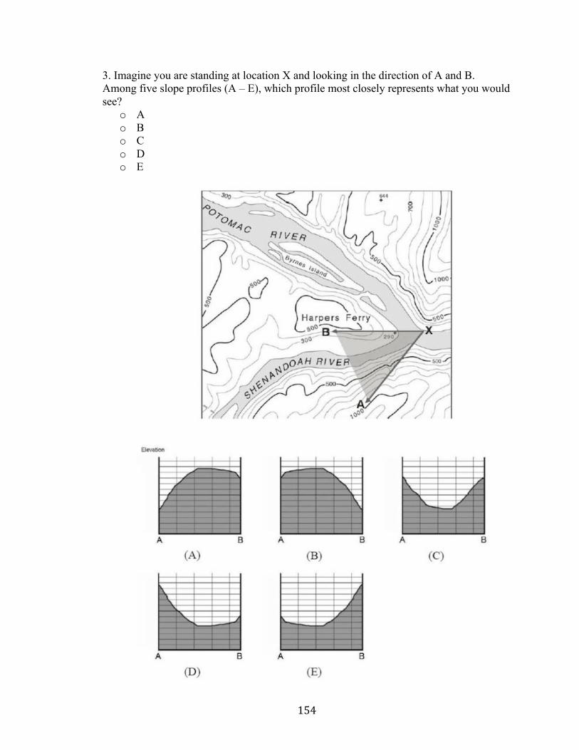
154

3. Imagine you are standing at location X and looking in the direction of A and B. Among five slope profiles (A – E), which profile most closely represents what you would see?

o A o B o C o D o E

155

4. The following two maps show production areas for (a) corn and (b) hogs and pigs. If you draw a graph showing the relationship between the general patterns of map (a) and map (b), which of the four graphs is the best?

o A o B o C o D

156

5. Find a map (A – F) having a strong positive correlation (association or showing similar pattern) with the top map on the right. Choose the closest one.

o A o B o C o D o E o F

157

Real-world objects can be represented by points, lines (arcs), and areas. Based on the examples in the figure below, classify the following spatial data in questions 6, 7, 8, and 9.

6. Location of weather stations in Washington County.

o Lines o Area o Points and Lines o Points

7. Mississippi River channels and their basins.

o Lines o Area o Points and Lines o Lines and Area

8. Shuttle bus routes and bus stops of the Lincoln Elementary School.

o Points o Area o Points and Lines o Points and Area

9. Places that can be reached by Franklin County fire engines in 5 minutes or less.

o Points o Lines o Area o Points and Areas

158

10. Find the best location for a flood management facility based on the following conditions. First, a possible site for a flood management facility should be within 60 feet of an existing electric line. Second, a possible site for a flood management facility should be located less than 220 feet in elevation. And last, a possible site for a flood management facility should be located in state park or public land. Choose the best site (A - E) for the flood management facility on the potential facility location map.

o A o B o C o D o E

159

APPENDIX B

INSTRUCTOR INTERVIEWS

1. Are you male or female?

2. What ethnic group do you belong to?

3. What is your highest degree in geography?

4. How long have you taught undergraduate geography courses?

5. What geospatial concepts do the students find difficult to understand, or are

difficult to explain and exemplify in class? On what geospatial concepts do the

students score low?

6. On what geospatial concepts do the students score high?

7. What strategies do you use to teach fundamental geospatial concepts?

8. Do you have any other thoughts regarding undergraduate students’ understanding

of geospatial concepts?

160

WORKS CITED

Agresti, A. 2002. Categorical data analysis, 2nd ed. New York: Wiley. Albert, W. S., and R. Golledge. 1999. The use of spatial cognitive abilities in

Geographical Information Systems: The map overlay operation. Transactions in GIS 3 (1): 7-21.

Allen, M. J. 1974. Sex differences in spatial problem-solving styles. Perceptual and

Motor Skills 39: 843-46. Anthamatten, P. 2010. Spatial thinking concepts in early grade-level geography

standards. Journal of Geography 109 (5): 169-80. Ardila, A., and S. Moreno. 2001. Neuropsychological evaluation in Aruaco Indians: An

exploratory study. Journal of the International Neuropsychological Society 7: 510–15.

Association of American Geographers (AAG). 2006. Spatial Thinking Ability Test.

http://home.ewha.ac.kr/~ziriboy/STAT.pdf. (last accessed February 20, 2013). Association of American Geographers (AAG) Guide. 2012. Guide to Geography

Programs in the Americas 2011-2012: AAG Handbook and Directory of Geographers. Washington, D.C.: AAG.

Baenninger, M., and N. Newcombe. 1989. The role of experience in spatial test

performance: A meta-analysis. Sex Roles 20: 327-44. Baker, T. 2012. Envisioning the spatial university. Esri Insider.

http://blogs.esri.com/esri/esri-insider/2012/07/23/envisioning-the-spatial-university/ (last accessed January 10, 2014).

Battersby, S., R. Golledge, and M. Marsh. 2006. Incidental learning of geospatial

concepts across grade levels: Map overlay. Journal of Geography 105 (4): 139-46.

Bearden, J. 2014. Chi-square test of independence.

http://www.geneseo.edu/~bearden/socl211/chisquareweb/chisquare.html (last accessed February 13, 2014).

Bednarz, S. W. 2004. Geographic information systems: A tool to support geography and

environmental education. GeoJournal 60 (2): 191–99. Blaut, J. M. 1991. Natural mapping. Transactions of the Institute of British Geographers

16 (1): 55-74.

161

Boduszek, D. 2014. Chi-square test of independence and McNemar test. http://webzoom.freewebs.com/danielboduszek/documents/Chi-square%20Test%20&%20McNemar%20Test%20-%20D.Boduszek.pdf (last accessed February 14, 2014).

Bodzin, A. M. 2011. The implementation of a Geospatial Information Technology (GIT)-

supported land use change curriculum with urban middle school learners to promote spatial thinking. Journal of Research in Science Teaching 48 (3): 281-300.

Brace, N., R. Kemp, and R. Snelgar. 2012. SPSS for psychologists. Hampshire, U.K.:

Macmillan Publishers Ltd. BRAIN Initiative. 2013. www.whitehouse.gov/share/brain-initiative (last accessed 22

November 2013). Brown, A. L., and R. A. Ferrara. 1985. Diagnosing zones of proximal development. In

Culture, Communication, and Cognition: Vygostkian Perspectives, ed. J. V. Wertsch, 275-305. Cambridge: Cambridge University Press.

Butt, G. 2001. Closing the gender gap in geography. Teaching Geography 26 (3): 145-47. Cherry, S. F. 1991. Action research: Factors influencing recognition of geographical

locations on a world map. ERIC Document Reproduction Service No. ED 343825.

Chow, T. E. 2012. Expert system. Lecture slides for Geocomputation (GEO 7364),

November 6. Texas State University-San Marcos. Cochran, K. F., and G. H. Wheatley. 1988. Ability and sex-related differences in

cognitive strategies on spatial tasks. Journal of General Psychology 116: 43-55. Cole, M. 1985. The zone of proximal development: Where culture and cognition create

each other. In Culture, Communication, and Cognition: Vygostkian Perspectives, ed. J. V. Wertsch, 146-61. Cambridge: Cambridge University Press.

Cubist. 2014. http://www.rulequest.com/cubist-win.html (last accessed February 11,

2014). Cutter, S. L., R. Golledge, and W. L. Graf. 2002. The big questions in geography. The

Professional Geographer 54 (3): 305-17. Daniel, W. W. 1990. Applied Nonparametric Statistics, 2nd ed. Pacific Grove: Duxbury

Thomson Learning.

162

DiBiase, D. 2013. There’s more to spatial thinking than you think. Esri Insider. http://blogs.esri.com/esri/esri-insider/2013/01/22/theres-more-to-spatial-thinking-than-you-think/#more-1782 (last accessed January 10, 2014).

Downs, R. 1994. The need for research in geography education: It would be nice to have

some data. Journal of Geography 93 (1): 57-60. Educational Theories. 2013. http://crescentok.com/staff/jaskew/isr/education/theories.htm

(last accessed April 30, 2013). Estaville, L. E., E. J. Montalvo, F. A. Akiwumi, W. C. Ray, and N. T. Huynh. 2010.

Teaching geography undergraduate courses: Active learning. In Geography Undergraduate Programs: Pathways to Success, ed. L. E. Estaville, 133-62. Washington, D. C.: National Council for Geographic Education.

Explorable 2013. http://explorable.com/students-t-test (last accessed June 4, 2013). Ferguson, G. A. 1954. On learning and human ability. Canadian Journal of Psychology

8: 95-112. Franeck, M. A., B. D. Nelson, R. H. Aron, and W. J. Bisard. 1993. The persistence of

selected geographic misconceptions: A study of junior high through undergraduate college students. Journal of Geography 93 (6): 247-53.

Funderstanding. 2013. http://www.funderstanding.com/educators/lev-vygotsky-and-

social-cognition/ (last accessed May 8, 2013). Geospatial Thinking Survey. 2012. https://www.surveymonkey.com/s/QSSQPB3 (last

accessed February 25, 2013). Gersmehl, P. J. 2012. The spatial brain and the common core. Paper presented at the

annual meeting of the National Council for Geographic Education, San Marcos, TX. October 5.

Gersmehl, P. J., and C. A. Gersmehl. 2007. Spatial thinking by young children:

Neurologic evidence for early development and “educability”. Journal of Geography 106 (5): 181-91.

——— 2007. Yes, spatial thinking is that complicated. Research in Geographic

Education 9 (2): 41-47. ——— 2006. Wanted: A concise list of neurologically defensible and assessable spatial

thinking skills. Research in Geographic Education 8: 5-38. Gilmartin, P., and J. C. Patton. 1984. Comparing the sexes on spatial abilities: Map use

skills. Annals of the Association of American Geographers 74 (4): 605-19.

163

Golledge, R. G. 2002. The nature of geographic knowledge. Annals of the Association of American Geographers 92 (1): 1-14.

——— 1996. Geographical theories. International Social Science Journal 48 (4): 461-

76. ——— 1995. Primitives of spatial knowledge. In Cognitive Aspects of Human-Computer

Interaction for GIS, ed. T. L. Nyerges, D. M. Mark, R. Laurini, and M. J. Egenhofer, 29-44. Dordrecht, The Netherlands: Kluwer Academic Publishers.

Golledge, R., M. Marsh, and S. Battersby. 2008. A conceptual framework for facilitating geospatial thinking. Annals of the Association of American Geographers 98 (2): 285-308.

——— 2008. Matching geospatial concepts with geographic educational needs.

Geographical Research 46 (1): 85-98. Goodchild, M. 2009. NeoGeography and the nature of geographic expertise. Journal of

Location Based Services 3 (2): 82-96. Hardwick, S. W., L. L. Bean, K. A. Alexander, and F. M. Shelley. 2000. Gender vs. sex

differences: Factors affecting performance in geographic education. Journal of Geography 99 (6): 238-44.

Harris, M. 1983. Culture, people, nature: An introduction to general anthropology, 3rd

ed. New York: Harper and Row. Henrie, R. L., R. H. Aron, B. D. Nelson, and D. A. Poole. 1997. Gender-related

knowledge variations within geography. Sex Roles 36 (9/10): 605-23. Hespanha, S. R., M. Goodchild, and D. G. Janelle. 2009. Spatial thinking and

technologies in the undergraduate social science classroom. Journal of Geography in Higher Education 33(1): 17-27.

Hooey, C. A., and T. J. Bailey. 2005. Journal writing and the development of spatial

thinking skills. Journal of Geography 104(6): 233-41. Huynh, N. T. and B. Sharpe. 2013. An assessment instrument to measure geospatial

thinking expertise. Journal of Geography 112 (1): 3-17. ——— 2009. The role of geospatial reasoning in effective GIS problem solving: K-16

education levels. Geomatica 63 (2): 119-28. Huynh, N. T., K. Verma, M. Patton, and N. Stamper. 2013. Learning to think

(geo)spatially through creative play. Paper presented at the annual meeting of the National Council for Geographic Education, Denver, CO. August 2.

164

Irvine, S. H. and J. W. Berry, eds. 1988. Human abilities in cultural context. New York: Cambridge University Press.

Isaacson, W. 2007. Einstein: His life and universe. New York: Simon and Schuster.

Ishikawa, T. 2013. Geospatial thinking and spatial ability: An empirical examination of knowledge and reasoning in geographical science. The Professional Geographer 65 (4): 636-46.

Jo, I., and S. W. Bednarz. 2009. Evaluating geography textbook questions from a spatial perspective: Using concepts of space, tools of representation, and cognitive processes to evaluate spatiality. Journal of Geography 108 (1): 4-13.

Jo, I., S. Bednarz, and S. Metoyer. 2010. Selecting and designing questions to facilitate spatial thinking. The Geography Teacher 7 (2): 49-55.

Kemp, J. 2008. Lost in space: On becoming spatially literate. Knowledge Quest 36 (4):

32-39. Kim, M. and R. Bednarz. 2013. Effects of a GIS course on self-assessment of spatial

habits of mind (SHOM). Journal of Geography 112 (4): 165-177. Kozulin, A. 2003. Psychological tools and mediated learning. In Vygotsky’s educational

theory in cultural context, eds. A. Kozulin, B. Gindis, V. S. Ageyev, and S. M. Miller, 15-38. Cambridge: Cambridge University Press.

Kozulin, A., B. Gindis, V. S. Ageyev, and S. M. Miller, eds. 2003. Vygotsky’s

educational theory in cultural context. Cambridge: Cambridge University Press. Laerd Statistics. 2014. https://statistics.laerd.com/statistical-guides/one-way-anova-

statistical-guide-4.php (last accessed January 26, 2014). Lambert, D. 2010. Geography education research and why it matters. International

Research in Geographical and Environmental Education 19 (2): 83-86. Lawton, C. A. 1994. Gender differences in way-finding strategies: Relationship to spatial

ability and spatial anxiety. Sex Roles 30 (11/12): 765-79. Learning-Theories 2013. http://www.learning-theories.com/vygotskys-social-learning-

theory.html (last accessed May 4, 2013). Lee, J. W. 2005. Effect of GIS Learning on Spatial Ability. PhD diss., Texas A&M

University. Lee, J., and R. Bednarz. 2012. Components of spatial thinking: Evidence from a Spatial

Thinking Ability Test. Journal of Geography 111 (1): 15-26.

165

——— 2009. Effect of GIS learning on spatial thinking. Journal of Geography in Higher Education 33(2): 183–98.

LeVasseur, M. L. 1999. Students’ knowledge of geography and geographic careers.

Journal of Geography 98 (6): 265-71. Levine, S. C., M. Vasilyeva, S. F. Lourenco, N. S. Newcombe, and J. Huttenlocher. 2005.

Socioeconomic status modifies the sex difference in spatial skill. Psychological Science 16 (11): 841-45.

Liben, L. S. 2006. Education for spatial thinking. In Handbook of Child Psychology.

Volume Four, Child Psychology in Practice, ed. K. A. Renninger, I. E. Sigel, W. Damon, and R. M. Lerner, 197-247. New York: John Wiley.

Lidz, C. S., and B. Gindis. 2003. Dynamic assessment of the evolving cognitive functions

in children. In Vygotsky’s educational theory in cultural context, eds. A. Kozulin, B. Gindis, V. S. Ageyev, and S. M. Miller, 99-116. Cambridge: Cambridge University Press.

Madsen, L. M., and C. Rump. 2012. Considerations of how to study learning processes

when students use GIS as an instrument for developing spatial thinking skills. Journal of Geography in Higher Education 36 (1): 97-116.

Mark, D. M., and S. M. Freundschuh. 1995. Spatial concepts and cognitive models for

geographic information use. In Cognitive Aspects of Human-Computer Interaction for GIS, ed. T. L. Nyerges, D. M. Mark, R. Laurini, and M. Egenhofer, 21-28. Dordrecht, The Netherlands: Kluwer Academic Publishers.

Marsh, M., R. Golledge, and S. E. Battersby. 2007. Geospatial concept understanding and

recognition in G6–college students: A preliminary argument for minimal GIS. Annals of the Association of American Geographers 97 (4): 696–712.

Monday, D., G. Klein, and S. Lee. 2005. The assumptions of ANOVA. http://www.slide

finder.net/t/the_assumptions_anova_dennis_monday/anova_assumptions/28336934 (last accessed June 3, 2013).

Montello, D. R. 1993. Scale and multiple psychologies of space. In Spatial information

theory: A theoretical basis for GIS (Lecture Notes in Computer Science 716), ed. A. U. Frank and I. Campari, 312-21. New York: Springer-Verlag.

Montello, D. R., K. L. Lovelace, R. G. Golledge, and C. M. Self. 1999. Sex-related

differences and similarities in geographic and environmental spatial abilities. Annals of the Association of American Geographers 89 (3): 515-34.

Mulenga, K., T. Ahonen, and M. Aro. 2001. Performance of Zambian children on the

NEPSY: A pilot study. Developmental Neuropsychology 20: 375–84.

166

National Council for Geographic Education. 2012. Geography for life: National geography standards, 2nd ed. Washington, D.C.: NCGE.

National Research Council. 2006. Learning to Think Spatially: GIS as a Support System

in the K-12 Curriculum. Washington, D. C.: National Academies Press. http://www.nap.edu/catalog.php?record_id=11019. (last accessed January 30, 2013).

Newcombe, N. S. 2010. Picture this: Increasing math and science learning by improving

spatial thinking. American Educator 34 (2): 29-43. Newcombe, N. S., and J. Huttenlocher. 2006. Development of spatial cognition. In

Handbook of Child Psychology. Volume Four, Child Psychology in Practice, ed. K. A. Renninger, I. E. Sigel, W. Damon, and R. M. Lerner, 734-76. New York: John Wiley.

Park, H. M. 2009. Comparing Group Means: T-tests and One-way ANOVA Using

STATA, SAS, R, and SPSS. http://www.indiana.edu/~statmath/stat/all/ttest (last accessed June 4, 2013).

Patton, M. Q. 2002. Qualitative Research and Evaluation Methods. Thousand Oaks, CA: Sage.

Perkins, N., E. Hazelton, J. Erickson, and W. Allan. 2010. Place-based education and

geographic information systems: Enhancing the spatial awareness of middle school students in Maine. Journal of Geography 109 (5): 213-18.

Portes, P. R., and J. A. Vadeboncoeur. 2003. Mediation in cognitive socialization: The

influence of socioeconomic status. In Vygotsky’s educational theory in cultural context, ed. A. Kozulin, B. Gindis, V. S. Ageyev, and S. M. Miller, 371-92. Cambridge: Cambridge University Press.

Rediscovering Geography Committee. 1997. Rediscovering Geography: New Relevance

for Science and Society. Washington, D.C.: National Academy Press. Rosselli, M., and A. Ardila. 2003. The impact of culture and education on non-verbal

neuropsychological measurements: A critical review. Brain and Cognition 52: 326-33.

Rowntree, L., M. Lewis, M. Price, and W. Wyckoff. 2014. Globalization and diversity:

geography of a changing world, 4th ed. Upper Saddle River: Pearson. SAS 2014. Principal component analysis.

support.sas.com/publishing/pubcat/chaps/55129.pdf (last accessed February 5, 2014).

167

Self, C. M., and R. G. Golledge. 1994. Sex-related differences in spatial ability: What every geography educator should know. Journal of Geography 93 (5): 234-42.

Sinton, D. S., S. Bednarz, P. Gersmehl, R. Kolvoord, and D. Uttal. 2013. The people’s

guide to spatial thinking. Washington, D. C.: National Council for Geographic Education.

Smith, J. 2007. Developing a spatial thinking skills taxonomy: Are there important

lessons to learn from Bloom? Research in Geographic Education 9 (2): 35-40. Solem, M., I. Cheung, and M. B. Schlemper. 2008. Skills in professional geography: An

assessment of workforce needs and expectations. The Professional Geographer 60 (3): 356-73.

Spence, I., J. J. Yu, J. Feng, and J. Marshman. 2009. Women match men when learning a

spatial skill. Journal of Experimental Psychology: Learning, Memory and Cognition 35(4): 1097-103.

Stat Trek. 2014. http://stattrek.com/chi-square-test/independence.aspx (last accessed

January 29, 2014). Stevens, J. 1986. Applied multivariate statistics for the social sciences. Hillsdale, NJ:

Lawrence Erlbaum Associates. Sword, L. 2001. I think in pictures, you teach in words: The gifted visual-spatial learner.

Tall Poppies Magazine. http://www.giftedchildren.org.nz/national/article4.php (last accessed February 28, 2011).

Tate, N. J., C. H. Jarvis, and K. E. Moore. 2005. Locating spatial thinking in teaching

practice. Computers, Environment and Urban Systems 29: 87-91. Uttal, D. H. 2000. Seeing the big picture: Map use and the development of spatial

cognition. Developmental Science 3 (3): 247-86. Uttal, D. H., N. G. Meadow, E. Tipton, L. L. Hand, A. R. Alden, C. Warren, and N.

Newcombe. 2013. The malleability of spatial skills: A meta-analysis of training studies. Psychological Bulletin 139 (2): 352-402.

U.S. Census Bureau. 2014. http://www.census.gov/geo/maps-data/data/tiger-cart-

boundary.html (last accessed January 27, 2014). Voyer, D., S. Voyer, and P. M. Bryden. 1995. Magnitude of sex differences in spatial

abilities: A meta-analysis and consideration of critical variables. Psychological Bulletin 117(2): 250-70.

168

Vygotsky, L. S. 1978. Mind in society: The development of higher psychological processes. Cambridge: Harvard University Press.

Wai, J. 2012. Why don’t we value spatial intelligence? Psychology Today.

http://www.psychologytoday.com/blog/finding-the-next-einstein/201203/why-dont-we-value-spatial-intelligence (last accessed January 10, 2014).

Walker, S. L., R. L. Bunch, O. Muniz, C. Murr, X. Qui, M. Rockeymoore, M. Warren,

and P. Wridt. 2005. Cognition and learning in geographic education: A research agenda. Research in Geographic Education 7: 21-31.

GEOSPATIAL THINKING OF UNDERGRADUATE STUDENTS IN …

Documents

Transcript of GEOSPATIAL THINKING OF UNDERGRADUATE STUDENTS IN …