Gender inequality, measurement and evidence

Gender inequality, measurement and evidence

Elena Bárcena-Martín

Universidad de Málaga Spain

Winter School on Inequality and Social Welfare Theory

Canazei, January 2018

1

• There still exist differences in economic status of men and women.

• Usual indicator of well-being: income.

• We find evidence of lower incomes of women.

2

0

2.000

4.000

6.000

8.000

10.000

12.000

14.000

16.000

18.000

2006 2007 2008 2009 2010 2011 2012 2013 2014 2015 2016

Median income EU(27)

Males Females

Source: Eurostat

3

At-risk-of-poverty rate by poverty threshold (60% median)

14,0

14,5

15,0

15,5

16,0

16,5

17,0

17,5

18,0

18,5

2006 2007 2008 2009 2010 2011 2012 2013 2014 2015 2016

Poverty

Males Females

Source: Eurostat

4

Individual vs. Household income in UK

Source: Lise and Seitz (2011)

16-65, no students, no retirees and no self-employed

∆ 12%

∆ 41%

5

Source: Lise and Seitz (2011)

Reduction in gender wage gap

Rise in female labour supply

Share of labour earnings that would be

contributed by the wife if both spouses worked

full-time

Large rise in inequality between households while a fall in inequality in the earnings distribution within households.

6

Outline

• 1. Measurement of individual income. Effects on the gender inequality measurement in the literature.

• 2. Information on intra-household distribution of resources: EUSILC 2010.

• Recent empirical applications for gender poverty gap in EU

• 3. How financial regimens (intra-household distribution of resources and decision responsibilities) affect deprivation levels.

7

• Difference between individual income and household incomes.

Individual information Wages, pensions

Household level information Capital income, transfers

• We know the resources of the household

• But not the exact level of income enjoyed by the person

• We know the resources of each individual

• But not the exact level of income enjoyed by the person

Assumptions are made on how incomes are distributed within the household

8

• Many influences from household and public spheres

Individual well-being

Public sphere:

institutios, policies,...

Labour market

Household: sharing,

allocation of time

9

• Three main types of income in the household:

Income from work

wages, salaries, profits, losses

Income from property

assets, rent, royalties

Income from state

unemployment benefits, pensions,…

family benefits, housing benefits, other benefits, child parental

support

Individual level

Householdlevel

Information on

ownership

10

• What is the exact gender gap in well-being? We need to account for individual well-being.

• We need information at household and individual level and about the interaction of individuals within the household.

• How to distribute household income between household members?

11

• Difficulty to get precise information on individual well-being: • Tradition of surveys aimed at households or individuals, not at both levels.

• Individual level data collection: complicated and costly.

• Difficult to know who benefits of household incomes (family benefits or capital incomes).

• Lack of information on the level of pooling of each individual: proportion of incomes kept apart for each individual.

• Not information on share of pooled incomes enjoyed by each individual.

12

Individual incomes from all HH members

are aggregated, resulting in HH

income

HH income is transformed in

equivalent income through equivalence

scales

Each individual in the HH is assumed to

receive have the same income, equal to the

HH equivalent income

Common “OECD‐modified” equivalence scale:

Weight 1 first adult member, 0.5 to an additional adult in the HH 0.3 to an additional child (younger than 14).

No intra-household inequality

Biased estimates of gender inequality because ignore intra-household inequality.

Assumption 1: all incomes received by household members are pooled

Assumption 2: pooled incomes are equally shared between household members

13

• Deriving individual income from household level information making assumptions of income pooling and equal sharing within the household.

• Ignores intra-household inequality (not in single-person households).

• Biased estimates of gender inequality.

14

Type of Household EU(27) (2016) % individuals

One person household 14.5 2 adults, no children, -65 13.2

2 adults, no children, one +65 12.1 Other HH no child 11.2

Single parent 4.7 2 adults +1 children 11.7 2 adults +2 children 15.9 2 adults +3 children 7.1

Other HH with children 9.6

85.5% of individuals in households in

which we ignore intra-

household inequality

Implications for the assessment of

inequality, especially between men and women

Source: Eurostat

15

Not the same % of single households in all countries. Different bias in inequality measurement per country

makes comparisons difficult.

Source: Eurostat 16

0

2

4

6

8

10

12

14

16

2007 2008 2009 2010 2011 2012 2013 2014 2015 2016

% population in single person households EU27

Increasing number of single person households

Reduction of bias. Still significant % of individuals in no single households

17

• What the standard approach ignores when attributing an equal standard of living to each member of a household? Jenkins (1991)

𝑤𝑖 earnings rate.

𝐿𝑀𝑖 time in labour market. 𝑁𝐿 couples non labour market.

𝑛𝑒𝑞 equivalent adults.

𝑓 females.

𝑚 males.

𝑌𝑒𝑞 =𝑤𝑓𝐿𝑀𝑓 +𝑤𝑚 𝐿𝑀𝑚 + 𝑁𝐿

𝑛𝑒𝑞

18

• Other possibilities:

• Many options depending on 𝑎1, 𝑏1, 𝑎2 , 𝑏2

Incomes not pooled

Incomes pooled

𝑌𝑒𝑞 = 𝑎1(𝑤𝑓𝐿𝑀𝑓) +𝑏1(𝑤𝑚 𝐿𝑀𝑚) + 𝑎2𝑁𝐿𝑓 + 𝑏2𝑁𝐿𝑚+

(1−𝑎1)(𝑤𝑓𝐿𝑀𝑓)+(1−𝑏1)(𝑤𝑚𝐿𝑀𝑚)+(1−𝑎2)𝑁𝐿𝑓+(1−𝑏2)𝑁𝐿𝑚

𝑛𝑒𝑞

19

Outline




• 3. How financial regimen (intra-household distribution of resources and decision responsibilities) affect deprivation levels.

20

• No much information on intra-household distribution of resources.

• EU statistics on income and living conditions (EU-SILC) 2010 EU-SILC module on ‘Intra-household sharing of resources’.

• Europeans (EU-27) that were living in households with at least two persons aged 16 years old and over.

21

full pooling 54%

Partial pooling

39%

no pooling 7%

Household pooling regimes based on individual responses, 2010

Note: Consistent responses only Source: Ponthieux (2013) Assumption of full income pooling

could be inappropriate

22

• Less likely to pool incomes: • Dual-earners couples

• Unmarried couples

• “Patchwork” families

• Full pooling likely to go down due to: • Decreasing marriage, increasing cohabitation.

• Increasing divorces and recomposed families.

• Increasing dual-earner households.

23

Full estimation of household allocation models:

• They adopt assumptions other than intra-household inequality. • Apply a form of minimal sharing restricted to the household’s non-labour income. • Assume unequal transfers of income between the household members. • Assume an unequal sharing of the household market income. • Use of microsimulation, making different pooling assumptions by source of income.

• All these studies concludes: • women’s shares of income tend to be dramatically lower, • women’s rank in the distribution of incomes sinks to the bottom quantiles, • women’s poverty risk rate is much higher whereas that of men is significantly

reduced.

• Therefore, there are implications on gender inequality measurement.

24

Income poverty rates are higher for women

25

Source: Ponthieux and Meurs (2015)

• Some recent contributions. Corsi et al. (2016) • Propose an individualized measure of European poverty to highlight gender

differences employing data from EU-SILC for the period 2007–2012.

• Consider adult individuals (over 18).

• Estimate at-risk-of-poverty rate.

26

• Assume that are kept apart

Individual incomes

• Assume that are equally shared

Household incomes

𝑌𝑒𝑞,𝑖 = 𝑦𝑖 +𝑌𝐶 − 𝑇

𝑛𝑒𝑞

Individual income

Household income equally

shared

27

Source: Corsi et al. (2016)

Share of incomes reported at the individual level is on average very high but lower for women than for men Women have lower resources of their own

Individualized incomes highlight substantial gender differences

Conventional

Individualized

28


For women the difference between FDRs and ARPRs is systematically dramatically larger than for men. Equal sharing of HH incomes assumption results in underestimation of gender gaps in poverty

ARPR: lower bound of the estimate of women’s poverty, under “optimistic” assumptions FDR: upper-bound estimate, under the “pessimistic” assumption of very little sharing of resources

Share of men and women whose individualized income is below 60% of their country’s median individualized income

29

Effect on the assessment of the role of state transfers


Decreasing trend in the gender gap, ARPR and FDR. Opposite conclusion: • STs reduce ARPR, and improve

gender equality. • STs reduce FDR but reduce gender

equality.

30

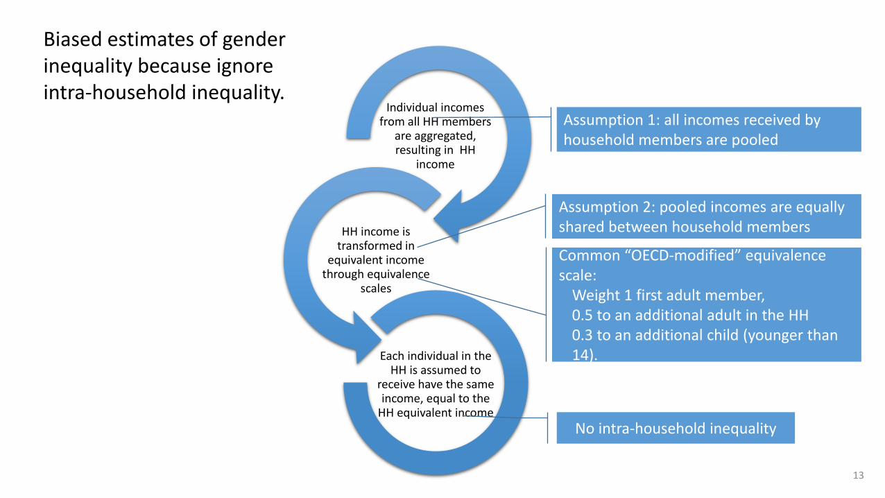
• Other recent contribution departing from full pooling: Ponthieux (2017)

• Use of EUSILC module 2010.

• Only couples (married or cohabitant, with or without children), i.e. households with a maximum of two decision-makers.

• Same sex couples are excluded.

31

Striking difference: proportion of women who report having

no personal income.

Source: Ponthieux (2017) 32

In 14 of the 21 countries the majority of couples correspond to the standard assumption of full income pooling.

But other pooling regimes are frequent enough

Source: Ponthieux (2017) 33

• Ponthieux (2017) principle of the ‘modified’ equivalised income consists of applying the standard approach, but only to the pooled income instead of the total disposable income.

• Conventional and ‘modified’ approaches are equivalent in the case of ‘full income pooling’ couples.

34

• Standard approach:

• Then 𝑌𝑒𝑞,𝑓 = 𝑌𝑒𝑞,𝑚 = 𝑌𝑒𝑞,𝐶ℎ = 𝑌𝑒𝑞


Individual incomes


Household incomes

𝑌𝑒𝑞 =𝑠𝑢𝑚 𝑜𝑓 𝑖𝑛𝑐𝑜𝑚𝑒𝑠 𝑓𝑟𝑜𝑚 𝐻𝐻 𝑚𝑒𝑚𝑏𝑒𝑟𝑠(𝐷)

𝑛𝑒𝑞

35

• Modified approach: personal incomes can be kept apart.

• Assume

SOME are kept apart, the rest are common and equally shared

Individual incomes


Household incomes

Separate incomes: 𝑦𝑓 + 𝑦𝑚

Pooled incomes: 𝑃 = (𝑌𝑓−𝑦𝑓) + (𝑌𝑚−𝑦𝑚) + 𝑌𝐶 − 𝑇

𝑌𝐶 common incomes 𝑇 social security contributions and taxes

Then:

𝑌𝑒𝑞,𝑃 =(𝑌𝑓−𝑦𝑓) + (𝑌𝑚−𝑦𝑚) + 𝑌𝐶 − 𝑇

𝑛𝑒𝑞

36

• Dealing with EU-SILC 2010 module data. • Separate income: 𝑦𝑖 that is the proportion of net income stated in the survey

• Contributed income: (𝑌𝑖−𝑦𝑖) that is the proportion of net income stated in the survey

• Then 𝑌𝑒𝑞,𝑓 = 𝑦𝑓 + 𝑌𝑒𝑞,𝑃

𝑌𝑒𝑞,𝑚 = 𝑦𝑚 + 𝑌𝑒𝑞,𝑃

𝑌𝑒𝑞,𝐶ℎ= 𝑌𝑒𝑞,𝑃

37

Source: Ponthieux (2017)

small difference

between the wives’

and husbands’

shares of modified equivalised income

38


Standard-modified

equivalised income

difference: intra-couple

differentials in personal

incomes are

counterbalanced by the

distribution of couples’

pooling regimes.

39


Women’s ‘modified’ poverty risk is higher than men’s. Deviating from the standard assumptions, by allowing for the possibility that incomes are not fully pooled, results in higher poverty risks for women than for men.

40

Conclusions

Results on the effect of intra-household distribution on income in the assessment of gender inequality reveals some limitations:

• Some income components are provided at household level and should be collected individual level to not incur in underestimation of gender inequalities. More individual-level information is encouraged.

• The use of equivalence scales assume equal sharing and ignores intra-household inequalities. Some alternatives should be tested.

• Policies that condition what an individual is entitled to with the resources of the household can reinforce inequalities between individuals and particularly the imbalance of resources between women and men. Recommendations for an individual-based right to social transfers is encouraged.

41

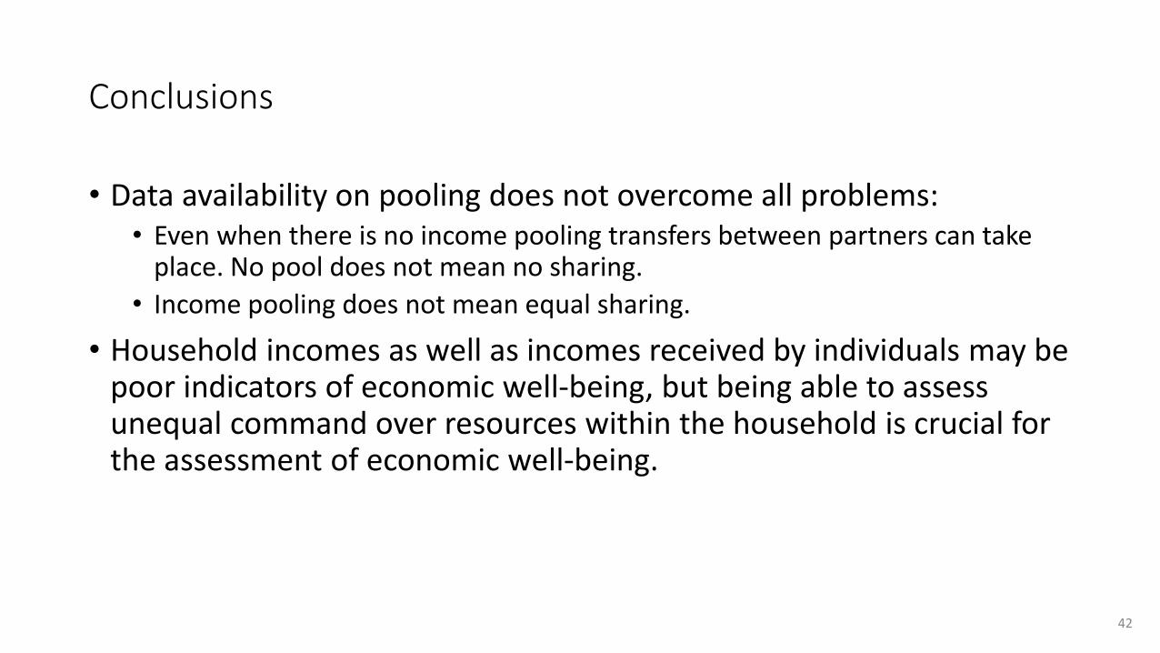
• Data availability on pooling does not overcome all problems: • Even when there is no income pooling transfers between partners can take

place. No pool does not mean no sharing.

• Income pooling does not mean equal sharing.

• Household incomes as well as incomes received by individuals may be poor indicators of economic well-being, but being able to assess unequal command over resources within the household is crucial for the assessment of economic well-being.

Conclusions

42

Outline




• 3. How financial regimen (intra-household distribution of resources and decision responsibilities) affect deprivation levels.

43

Implications of intra-household allocation of resources on the level of deprivation

• Bárcena-Martín, E., Blázquez, M. and Moro-Egido, A. (2017) Intra-household allocation of resources and household deprivation, Working Papers in Economic Theory 2017/03.

• Individuals with the same household income may suffer different deprivation levels.

• Analysis of the impact of different household financial regimes on deprivation in a number of European countries.

• Special module on intra-household sharing of resources included in the 2010 wave of EU-SILC dataset.

44

https://ideas.repec.org/p/uam/wpaper/201703.html



• Since the family involves an intra-household scheme of exchange and distribution of resources, different financial regimes within the household may, to some extent, explain the presence of specific types and levels of deprivation

• Empirical evidence suggests:

• Individuals may have different preferences and may not pool their incomes.

• Decision-making process in a family exerts an important influence on the intra-household dynamics and welfare of the household.

45

Literature review

Individual and household determinants of deprivation: • Negative and weak relationship with income. • Families with dependent children are especially vulnerable to

material deprivation. • No clear relationship with age (if any U-shaped). • Higher education reduces deprivation. • Households with one or more self-employed or employed

workers generally present lower deprivation scores.

46

Literature review

• Studies rely on the assumption that family members act as if they maximize a single utility function (Samuelson, 1956; Becker, 1981), and thus ignored the potential for unequal power and resource distribution within households.

• Recent empirical studies suggest that the unitary approach is not always supported and that significant inequalities might exist within the same family (see, for instance, Fortin and Lacroix, 1997; Clark et al., 2002 and Ward-Batts, 2008; Dietrich, 2008 for China; Bonke and Uldall-Poulsen, 2005; among others).

47

Literature review

• New literature based on non-unitary models (mainly collective models)

• Each household member is characterized by his or her own utility function.

• Decisions are seen as the outcome of some bargaining process (Bourguignon and Chiappori, 1992; Chiappori, 1992, 1997).

• An important distinction has been made between responsibility for the management of household resources and control of (major) household decisions (Pahl, 1989; Wilson, 1987).

48

Deprivation Household Intrahousehold distribution of

resources

Different decisions making

responsabilities

Financial regimes

Intrahousehold distribution of

resources

Different decisions making

responsibilities

49

Data

• The 2010 module on intra-household sharing of resources of the EUSILC.

• Sample: heterosexual couples, with or without children, for 24 countries.

• We eliminate couples with inconsistent responses on the decision-making variables.

• We end up with 84,269 observations.

50

Deprivation

• Di : Deprivation Index (12 Items) (Guio et al., 2009) • Economic strain: to keep home adequately warm; to afford paying for

one-week annual holiday away from home; to afford a meal with meat, chicken, fish every second day; to face unexpected financial expenses.

• Durables: to have a telephone; a color TV; a computer; a washing machine; a personal car.

• Housing: to have leaking roof/damp walls/floors/foundation or rot in window frames; no bath/shower; no indoor flushing toilet for sole use of the household.

51

• Di : Deprivation Index (Aggregation)

for each item we define a dichotomous indicator Iij:

and deprivation level is:

that equals 0 if a person lacks no items and increases with the number of items the individual lacks.

,....,Jj,...,N;ifor

abilitynon afford

ity affordabilIij 11

1

0

J

j

ijji IwD1

Deprivation

52

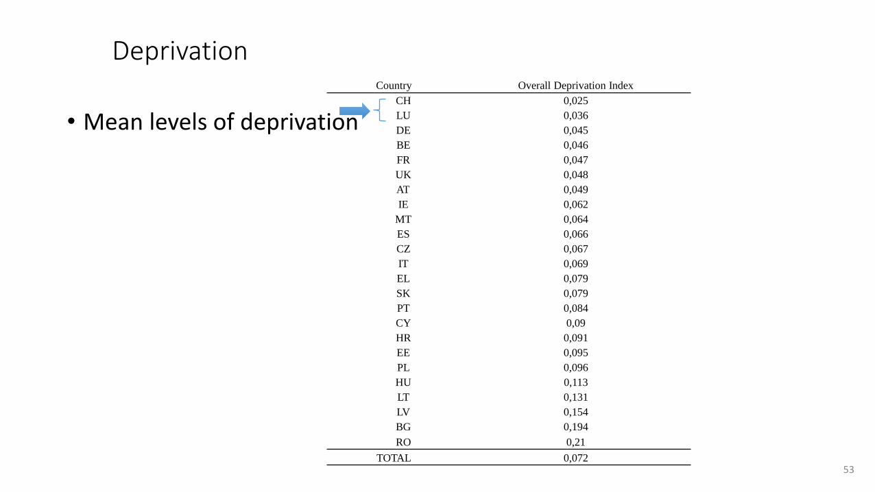
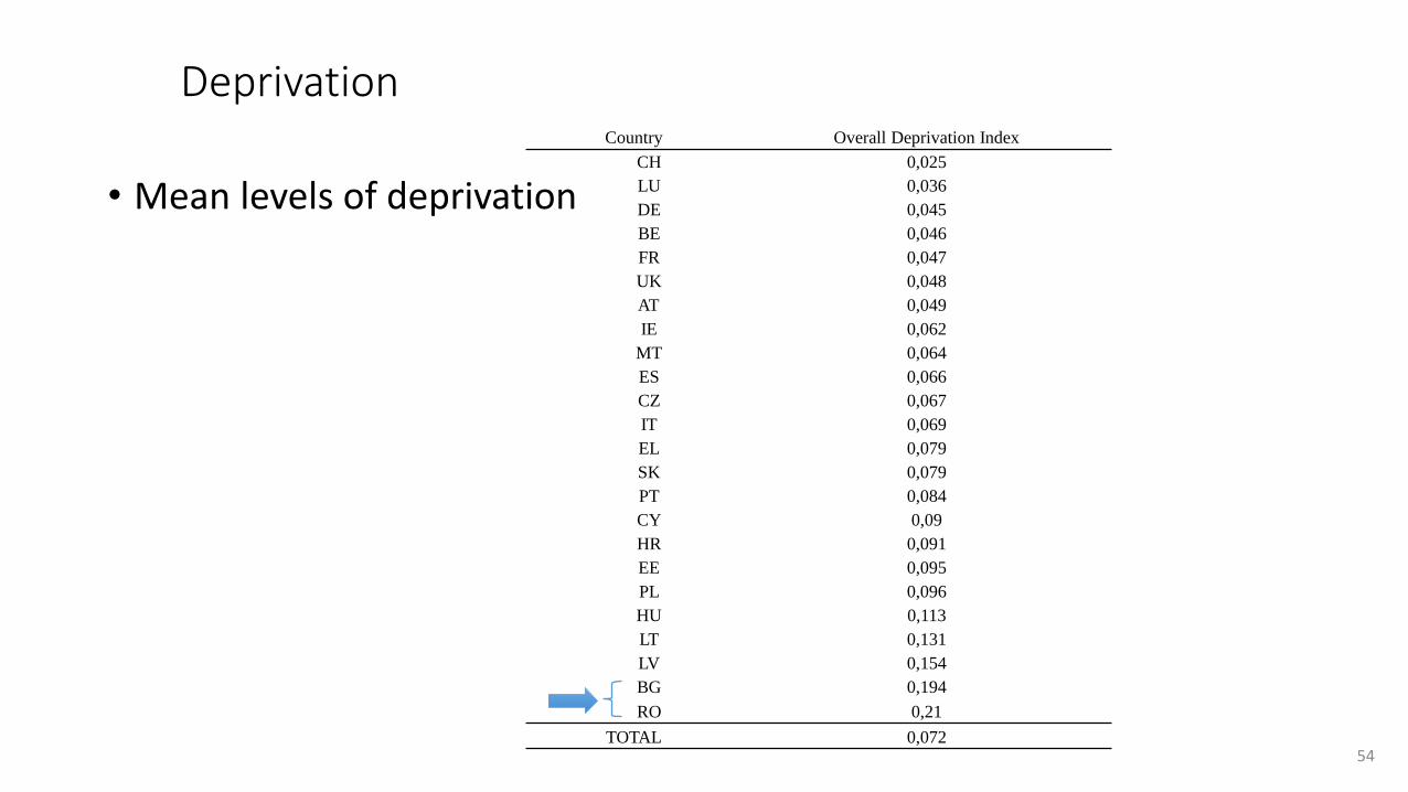
Deprivation

• Mean levels of deprivation

Country Overall Deprivation Index

CH 0,025

LU 0,036

DE 0,045

BE 0,046

FR 0,047

UK 0,048

AT 0,049

IE 0,062

MT 0,064

ES 0,066

CZ 0,067

IT 0,069

EL 0,079

SK 0,079

PT 0,084

CY 0,09

HR 0,091

EE 0,095

PL 0,096

HU 0,113

LT 0,131

LV 0,154

BG 0,194

RO 0,21

TOTAL 0,072 53

Deprivation

• Mean levels of deprivation

Country Overall Deprivation Index

CH 0,025

LU 0,036

DE 0,045

BE 0,046

FR 0,047

UK 0,048

AT 0,049

IE 0,062

MT 0,064

ES 0,066

CZ 0,067

IT 0,069

EL 0,079

SK 0,079

PT 0,084

CY 0,09

HR 0,091

EE 0,095

PL 0,096

HU 0,113

LT 0,131

LV 0,154

BG 0,194

RO 0,21

TOTAL 0,072 54

The Model

• Zi : Socioeconomic variables

• Income: household annual equivalent disposable income

• Child: dummy to identify the presence of children

• Dual: both members of the couple are working either full or part time

• H_Young: when the mean age of the couple is less than 35

• H_Middle: when the mean age of the couple is from 35 to 65

• H_Old (reference category)

• H_Tertiary and H_Secondary : 0 if None of the members of the couple have tertiary education or secondary education; 1 if only one of them has tertiary or secondary education; and 2 if both have tertiary or secondary education.

• H_Chronic: number of household members suffering from chronic diseases.

• H-Marital: dummy for legal consensual unions

iiD 3210

'i

'i

'i CZW

55

The Model

• Ci : Country specific fixed effects

iiD 3210

'i

'i

'i CZW

56

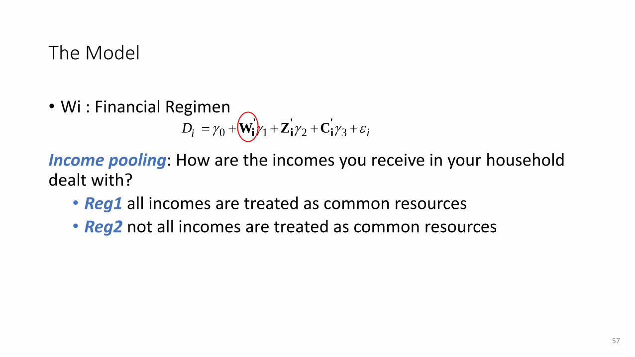
The Model

• Wi : Financial Regimen

Income pooling: How are the incomes you receive in your household dealt with?

• Reg1 all incomes are treated as common resources

• Reg2 not all incomes are treated as common resources

iiD 3210

'i

'i

'i CZW

57

The Model


Financial decision-making: "Who in your couple is generally more likely to take decisions on" in five areas: i) shopping; ii) children expenses; iii) furniture, etc.; iv) borrowing; v) saving

• Dec_f if females have most decision-making responsibilities

• Dec_m if males have most decision-making responsibilities

• Dec_s if decisions are shared

iiD 3210

'i

'i

'i CZW

58

The Model


Financial decision-making: Watson et al. (2013):

• The average across the items that range from 0 (responsibility for decision making in none of the areas) to 10 (responsibility for decision making in all areas).

• A score from 4 to 6 shared responsibility • adults are jointly responsible for each of the areas

• an almost even division of responsibilities between them (e.g., one is responsible for shopping and the other is responsible for decisions on savings).

iiD 3210

'i

'i

'i CZW

59

The Model

Wi : Financial Regimen

iiD 3210

'i

'i

'i CZW

Variable Description Mean values

Reg1_DecS All income pooling and decisions shared (Reference) 41,66%

Reg1_DecF All income pooling and decisions mainly female 31,58%

Reg1_DecM All income pooling and decisions mainly male 5,42%

Reg2_DecS Not All income pooling and decisions shared 9,46%

Reg2_DecF Not All income pooling and decisions mainly female 9,74%

Reg2_DecM Not All income pooling and decisions mainly male 2,15%

60

The Model

Linear model. Cluster robust standard errors

Wi : Financial Regimen Endogeneity problem

Deb and Trivedi (2006) : Two set of equations:

Choice of financial regime (selection)

Intensity of deprivation (outcome).

(The selection and the outcome equations are linked via observed and unobserved characteristics).

iiD 3210

'i

'i

'i CZW

61

The Model

Deb and Trivedi (2006) :

Selection equation

• multinomial choice model for the household financial regimen (selection)

• Let denote the indirect utility associated with the jth choice (j=1,…J)

• Xi includes the exogenous variables plus the instruments

• mik, incorporate unobserved characteristics common to deprivation and household decisions regarding the financial regimen (independent of ij)

• ij are i.i.d. error terms

Uij

*

Uij

* = X i

'b j + j jkmik

k=1

J

å +hij

62

The Model


Selection equation

• Let bj be the binary variables representing the observed choices

• The probability of any type of financial regime can be represented as:

where g is a multinomial probability distribution

Some restrictions are imposed: each choice is affected by a unique latent factor

bi = bi1,bi 2,...,biJ[ ]Pr(bi X i,M i ) = g X i

'b1 + j1kmik

k=1

J

å , X i

' b2 + j2kmik

k=1

J

å , ... , X i

' bJ + jJkmik

k=1

J

åæ

èç

ö

ø÷

63

The Model


Outcome equation

Where:

• is the set of exogenous covariates

• denotes the selection effects relative to the control

Di =g0 + d jbij

j=1

J

å + l jmij

j=1

J

å + Z i

'g2 +Ci

'g3 +ei

Z i

d j

64

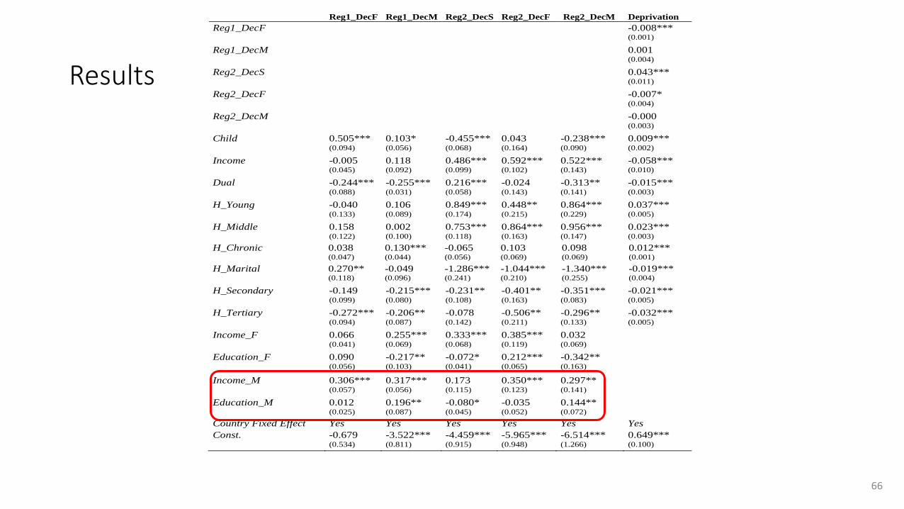
Results Validity of instruments

• Instruments: measure within-household inequalities concerning education and income (following Vogler (1994), Lyngstad et al. (2011), and Mader and Schneebaum (2013)).

• Income_F and Income_M: Dummies to capture female or male earning more income than her/his partner

• Education_F and Education_M: Dummies to capture female or male with higher level of education than her/his partner

• They have useful predictive power and hence are relevant.

• We test for the exogeneity of the financial regimes, and they are not exogenous.

65

Results

Reg1_DecF Reg1_DecM Reg2_DecS Reg2_DecF Reg2_DecM Deprivation

Reg1_DecF

-0.008*** (0.001)

Reg1_DecM

0.001 (0.004)

Reg2_DecS

0.043*** (0.011)

Reg2_DecF

-0.007* (0.004)

Reg2_DecM

-0.000 (0.003)

Child 0.505*** 0.103* -0.455*** 0.043 -0.238*** 0.009*** (0.094) (0.056) (0.068) (0.164) (0.090) (0.002)

Income -0.005 0.118 0.486*** 0.592*** 0.522*** -0.058*** (0.045) (0.092) (0.099) (0.102) (0.143) (0.010)

Dual -0.244*** -0.255*** 0.216*** -0.024 -0.313** -0.015*** (0.088) (0.031) (0.058) (0.143) (0.141) (0.003)

H_Young -0.040 0.106 0.849*** 0.448** 0.864*** 0.037*** (0.133) (0.089) (0.174) (0.215) (0.229) (0.005)

H_Middle 0.158 0.002 0.753*** 0.864*** 0.956*** 0.023*** (0.122) (0.100) (0.118) (0.163) (0.147) (0.003)

H_Chronic 0.038 0.130*** -0.065 0.103 0.098 0.012*** (0.047) (0.044) (0.056) (0.069) (0.069) (0.001)

H_Marital 0.270** -0.049 -1.286*** -1.044*** -1.340*** -0.019*** (0.118) (0.096) (0.241) (0.210) (0.255) (0.004)

H_Secondary -0.149 -0.215*** -0.231** -0.401** -0.351*** -0.021*** (0.099) (0.080) (0.108) (0.163) (0.083) (0.005)

H_Tertiary -0.272*** -0.206** -0.078 -0.506** -0.296** -0.032*** (0.094) (0.087) (0.142) (0.211) (0.133) (0.005)

Income_F 0.066 0.255*** 0.333*** 0.385*** 0.032

(0.041) (0.069) (0.068) (0.119) (0.069)

Education_F 0.090 -0.217** -0.072* 0.212*** -0.342**

(0.056) (0.103) (0.041) (0.065) (0.163)

Income_M 0.306*** 0.317*** 0.173 0.350*** 0.297**

(0.057) (0.056) (0.115) (0.123) (0.141)

Education_M 0.012 0.196** -0.080* -0.035 0.144**

(0.025) (0.087) (0.045) (0.052) (0.072)

Country Fixed Effect Yes Yes Yes Yes Yes Yes

Const. -0.679 -3.522*** -4.459*** -5.965*** -6.514*** 0.649*** (0.534) (0.811) (0.915) (0.948) (1.266) (0.100)

66

Results


Reg1_DecF

-0.008*** (0.001)

Reg1_DecM

0.001 (0.004)

Reg2_DecS

0.043*** (0.011)

Reg2_DecF

-0.007* (0.004)

Reg2_DecM

-0.000 (0.003)

Child 0.505*** 0.103* -0.455*** 0.043 -0.238*** 0.009*** (0.094) (0.056) (0.068) (0.164) (0.090) (0.002)

Income -0.005 0.118 0.486*** 0.592*** 0.522*** -0.058*** (0.045) (0.092) (0.099) (0.102) (0.143) (0.010)

Dual -0.244*** -0.255*** 0.216*** -0.024 -0.313** -0.015*** (0.088) (0.031) (0.058) (0.143) (0.141) (0.003)

H_Young -0.040 0.106 0.849*** 0.448** 0.864*** 0.037*** (0.133) (0.089) (0.174) (0.215) (0.229) (0.005)

H_Middle 0.158 0.002 0.753*** 0.864*** 0.956*** 0.023*** (0.122) (0.100) (0.118) (0.163) (0.147) (0.003)

H_Chronic 0.038 0.130*** -0.065 0.103 0.098 0.012*** (0.047) (0.044) (0.056) (0.069) (0.069) (0.001)

H_Marital 0.270** -0.049 -1.286*** -1.044*** -1.340*** -0.019*** (0.118) (0.096) (0.241) (0.210) (0.255) (0.004)

H_Secondary -0.149 -0.215*** -0.231** -0.401** -0.351*** -0.021*** (0.099) (0.080) (0.108) (0.163) (0.083) (0.005)

H_Tertiary -0.272*** -0.206** -0.078 -0.506** -0.296** -0.032*** (0.094) (0.087) (0.142) (0.211) (0.133) (0.005)

Income_F 0.066 0.255*** 0.333*** 0.385*** 0.032

(0.041) (0.069) (0.068) (0.119) (0.069)

Education_F 0.090 -0.217** -0.072* 0.212*** -0.342**

(0.056) (0.103) (0.041) (0.065) (0.163)

Income_M 0.306*** 0.317*** 0.173 0.350*** 0.297**

(0.057) (0.056) (0.115) (0.123) (0.141)

Education_M 0.012 0.196** -0.080* -0.035 0.144**

(0.025) (0.087) (0.045) (0.052) (0.072)


Const. -0.679 -3.522*** -4.459*** -5.965*** -6.514*** 0.649*** (0.534) (0.811) (0.915) (0.948) (1.266) (0.100)

67

Results


Reg1_DecF

-0.008*** (0.001)

Reg1_DecM

0.001 (0.004)

Reg2_DecS

0.043*** (0.011)

Reg2_DecF

-0.007* (0.004)

Reg2_DecM

-0.000 (0.003)

Child 0.505*** 0.103* -0.455*** 0.043 -0.238*** 0.009*** (0.094) (0.056) (0.068) (0.164) (0.090) (0.002)

Income -0.005 0.118 0.486*** 0.592*** 0.522*** -0.058*** (0.045) (0.092) (0.099) (0.102) (0.143) (0.010)

Dual -0.244*** -0.255*** 0.216*** -0.024 -0.313** -0.015*** (0.088) (0.031) (0.058) (0.143) (0.141) (0.003)

H_Young -0.040 0.106 0.849*** 0.448** 0.864*** 0.037*** (0.133) (0.089) (0.174) (0.215) (0.229) (0.005)

H_Middle 0.158 0.002 0.753*** 0.864*** 0.956*** 0.023*** (0.122) (0.100) (0.118) (0.163) (0.147) (0.003)

H_Chronic 0.038 0.130*** -0.065 0.103 0.098 0.012*** (0.047) (0.044) (0.056) (0.069) (0.069) (0.001)

H_Marital 0.270** -0.049 -1.286*** -1.044*** -1.340*** -0.019*** (0.118) (0.096) (0.241) (0.210) (0.255) (0.004)

H_Secondary -0.149 -0.215*** -0.231** -0.401** -0.351*** -0.021*** (0.099) (0.080) (0.108) (0.163) (0.083) (0.005)

H_Tertiary -0.272*** -0.206** -0.078 -0.506** -0.296** -0.032*** (0.094) (0.087) (0.142) (0.211) (0.133) (0.005)

Income_F 0.066 0.255*** 0.333*** 0.385*** 0.032

(0.041) (0.069) (0.068) (0.119) (0.069)

Education_F 0.090 -0.217** -0.072* 0.212*** -0.342**

(0.056) (0.103) (0.041) (0.065) (0.163)

Income_M 0.306*** 0.317*** 0.173 0.350*** 0.297**

(0.057) (0.056) (0.115) (0.123) (0.141)

Education_M 0.012 0.196** -0.080* -0.035 0.144**

(0.025) (0.087) (0.045) (0.052) (0.072)


Const. -0.679 -3.522*** -4.459*** -5.965*** -6.514*** 0.649*** (0.534) (0.811) (0.915) (0.948) (1.266) (0.100)

68

Results


Reg1_DecF

-0.008*** (0.001)

Reg1_DecM

0.001 (0.004)

Reg2_DecS

0.043*** (0.011)

Reg2_DecF

-0.007* (0.004)

Reg2_DecM

-0.000 (0.003)

Child 0.505*** 0.103* -0.455*** 0.043 -0.238*** 0.009*** (0.094) (0.056) (0.068) (0.164) (0.090) (0.002)

Income -0.005 0.118 0.486*** 0.592*** 0.522*** -0.058*** (0.045) (0.092) (0.099) (0.102) (0.143) (0.010)

Dual -0.244*** -0.255*** 0.216*** -0.024 -0.313** -0.015*** (0.088) (0.031) (0.058) (0.143) (0.141) (0.003)

H_Young -0.040 0.106 0.849*** 0.448** 0.864*** 0.037*** (0.133) (0.089) (0.174) (0.215) (0.229) (0.005)

H_Middle 0.158 0.002 0.753*** 0.864*** 0.956*** 0.023*** (0.122) (0.100) (0.118) (0.163) (0.147) (0.003)

H_Chronic 0.038 0.130*** -0.065 0.103 0.098 0.012*** (0.047) (0.044) (0.056) (0.069) (0.069) (0.001)

H_Marital 0.270** -0.049 -1.286*** -1.044*** -1.340*** -0.019*** (0.118) (0.096) (0.241) (0.210) (0.255) (0.004)

H_Secondary -0.149 -0.215*** -0.231** -0.401** -0.351*** -0.021*** (0.099) (0.080) (0.108) (0.163) (0.083) (0.005)

H_Tertiary -0.272*** -0.206** -0.078 -0.506** -0.296** -0.032*** (0.094) (0.087) (0.142) (0.211) (0.133) (0.005)

Income_F 0.066 0.255*** 0.333*** 0.385*** 0.032

(0.041) (0.069) (0.068) (0.119) (0.069)

Education_F 0.090 -0.217** -0.072* 0.212*** -0.342**

(0.056) (0.103) (0.041) (0.065) (0.163)

Income_M 0.306*** 0.317*** 0.173 0.350*** 0.297**

(0.057) (0.056) (0.115) (0.123) (0.141)

Education_M 0.012 0.196** -0.080* -0.035 0.144**

(0.025) (0.087) (0.045) (0.052) (0.072)


Const. -0.679 -3.522*** -4.459*** -5.965*** -6.514*** 0.649*** (0.534) (0.811) (0.915) (0.948) (1.266) (0.100)

69

Results


Reg1_DecF

-0.008*** (0.001)

Reg1_DecM

0.001 (0.004)

Reg2_DecS

0.043*** (0.011)

Reg2_DecF

-0.007* (0.004)

Reg2_DecM

-0.000 (0.003)

Child 0.505*** 0.103* -0.455*** 0.043 -0.238*** 0.009*** (0.094) (0.056) (0.068) (0.164) (0.090) (0.002)

Income -0.005 0.118 0.486*** 0.592*** 0.522*** -0.058*** (0.045) (0.092) (0.099) (0.102) (0.143) (0.010)

Dual -0.244*** -0.255*** 0.216*** -0.024 -0.313** -0.015*** (0.088) (0.031) (0.058) (0.143) (0.141) (0.003)

H_Young -0.040 0.106 0.849*** 0.448** 0.864*** 0.037*** (0.133) (0.089) (0.174) (0.215) (0.229) (0.005)

H_Middle 0.158 0.002 0.753*** 0.864*** 0.956*** 0.023*** (0.122) (0.100) (0.118) (0.163) (0.147) (0.003)

H_Chronic 0.038 0.130*** -0.065 0.103 0.098 0.012*** (0.047) (0.044) (0.056) (0.069) (0.069) (0.001)

H_Marital 0.270** -0.049 -1.286*** -1.044*** -1.340*** -0.019*** (0.118) (0.096) (0.241) (0.210) (0.255) (0.004)

H_Secondary -0.149 -0.215*** -0.231** -0.401** -0.351*** -0.021*** (0.099) (0.080) (0.108) (0.163) (0.083) (0.005)

H_Tertiary -0.272*** -0.206** -0.078 -0.506** -0.296** -0.032*** (0.094) (0.087) (0.142) (0.211) (0.133) (0.005)

Income_F 0.066 0.255*** 0.333*** 0.385*** 0.032

(0.041) (0.069) (0.068) (0.119) (0.069)

Education_F 0.090 -0.217** -0.072* 0.212*** -0.342**

(0.056) (0.103) (0.041) (0.065) (0.163)

Income_M 0.306*** 0.317*** 0.173 0.350*** 0.297**

(0.057) (0.056) (0.115) (0.123) (0.141)

Education_M 0.012 0.196** -0.080* -0.035 0.144**

(0.025) (0.087) (0.045) (0.052) (0.072)


Const. -0.679 -3.522*** -4.459*** -5.965*** -6.514*** 0.649*** (0.534) (0.811) (0.915) (0.948) (1.266) (0.100)

70

Results


Reg1_DecF

-0.008*** (0.001)

Reg1_DecM

0.001 (0.004)

Reg2_DecS

0.043*** (0.011)

Reg2_DecF

-0.007* (0.004)

Reg2_DecM

-0.000 (0.003)

Child 0.505*** 0.103* -0.455*** 0.043 -0.238*** 0.009*** (0.094) (0.056) (0.068) (0.164) (0.090) (0.002)

Income -0.005 0.118 0.486*** 0.592*** 0.522*** -0.058*** (0.045) (0.092) (0.099) (0.102) (0.143) (0.010)

Dual -0.244*** -0.255*** 0.216*** -0.024 -0.313** -0.015*** (0.088) (0.031) (0.058) (0.143) (0.141) (0.003)

H_Young -0.040 0.106 0.849*** 0.448** 0.864*** 0.037*** (0.133) (0.089) (0.174) (0.215) (0.229) (0.005)

H_Middle 0.158 0.002 0.753*** 0.864*** 0.956*** 0.023*** (0.122) (0.100) (0.118) (0.163) (0.147) (0.003)

H_Chronic 0.038 0.130*** -0.065 0.103 0.098 0.012*** (0.047) (0.044) (0.056) (0.069) (0.069) (0.001)

H_Marital 0.270** -0.049 -1.286*** -1.044*** -1.340*** -0.019*** (0.118) (0.096) (0.241) (0.210) (0.255) (0.004)

H_Secondary -0.149 -0.215*** -0.231** -0.401** -0.351*** -0.021*** (0.099) (0.080) (0.108) (0.163) (0.083) (0.005)

H_Tertiary -0.272*** -0.206** -0.078 -0.506** -0.296** -0.032*** (0.094) (0.087) (0.142) (0.211) (0.133) (0.005)

Income_F 0.066 0.255*** 0.333*** 0.385*** 0.032

(0.041) (0.069) (0.068) (0.119) (0.069)

Education_F 0.090 -0.217** -0.072* 0.212*** -0.342**

(0.056) (0.103) (0.041) (0.065) (0.163)

Income_M 0.306*** 0.317*** 0.173 0.350*** 0.297**

(0.057) (0.056) (0.115) (0.123) (0.141)

Education_M 0.012 0.196** -0.080* -0.035 0.144**

(0.025) (0.087) (0.045) (0.052) (0.072)


Const. -0.679 -3.522*** -4.459*** -5.965*** -6.514*** 0.649*** (0.534) (0.811) (0.915) (0.948) (1.266) (0.100)

71


Reg1_DecF

-0.008*** (0.001)

Reg1_DecM

0.001 (0.004)

Reg2_DecS

0.043*** (0.011)

Reg2_DecF

-0.007* (0.004)

Reg2_DecM

-0.000 (0.003)

Child 0.505*** 0.103* -0.455*** 0.043 -0.238*** 0.009*** (0.094) (0.056) (0.068) (0.164) (0.090) (0.002)

Income -0.005 0.118 0.486*** 0.592*** 0.522*** -0.058*** (0.045) (0.092) (0.099) (0.102) (0.143) (0.010)

Dual -0.244*** -0.255*** 0.216*** -0.024 -0.313** -0.015*** (0.088) (0.031) (0.058) (0.143) (0.141) (0.003)

H_Young -0.040 0.106 0.849*** 0.448** 0.864*** 0.037*** (0.133) (0.089) (0.174) (0.215) (0.229) (0.005)

H_Middle 0.158 0.002 0.753*** 0.864*** 0.956*** 0.023*** (0.122) (0.100) (0.118) (0.163) (0.147) (0.003)

H_Chronic 0.038 0.130*** -0.065 0.103 0.098 0.012*** (0.047) (0.044) (0.056) (0.069) (0.069) (0.001)

H_Marital 0.270** -0.049 -1.286*** -1.044*** -1.340*** -0.019*** (0.118) (0.096) (0.241) (0.210) (0.255) (0.004)

H_Secondary -0.149 -0.215*** -0.231** -0.401** -0.351*** -0.021*** (0.099) (0.080) (0.108) (0.163) (0.083) (0.005)

H_Tertiary -0.272*** -0.206** -0.078 -0.506** -0.296** -0.032*** (0.094) (0.087) (0.142) (0.211) (0.133) (0.005)

Income_F 0.066 0.255*** 0.333*** 0.385*** 0.032

(0.041) (0.069) (0.068) (0.119) (0.069)

Education_F 0.090 -0.217** -0.072* 0.212*** -0.342**

(0.056) (0.103) (0.041) (0.065) (0.163)

Income_M 0.306*** 0.317*** 0.173 0.350*** 0.297**

(0.057) (0.056) (0.115) (0.123) (0.141)

Education_M 0.012 0.196** -0.080* -0.035 0.144**

(0.025) (0.087) (0.045) (0.052) (0.072)


Const. -0.679 -3.522*** -4.459*** -5.965*** -6.514*** 0.649*** (0.534) (0.811) (0.915) (0.948) (1.266) (0.100)

Results

72


Reg1_DecF

-0.008*** (0.001)

Reg1_DecM

0.001 (0.004)

Reg2_DecS

0.043*** (0.011)

Reg2_DecF

-0.007* (0.004)

Reg2_DecM

-0.000 (0.003)

Child 0.505*** 0.103* -0.455*** 0.043 -0.238*** 0.009*** (0.094) (0.056) (0.068) (0.164) (0.090) (0.002)

Income -0.005 0.118 0.486*** 0.592*** 0.522*** -0.058*** (0.045) (0.092) (0.099) (0.102) (0.143) (0.010)

Dual -0.244*** -0.255*** 0.216*** -0.024 -0.313** -0.015*** (0.088) (0.031) (0.058) (0.143) (0.141) (0.003)

H_Young -0.040 0.106 0.849*** 0.448** 0.864*** 0.037*** (0.133) (0.089) (0.174) (0.215) (0.229) (0.005)

H_Middle 0.158 0.002 0.753*** 0.864*** 0.956*** 0.023*** (0.122) (0.100) (0.118) (0.163) (0.147) (0.003)

H_Chronic 0.038 0.130*** -0.065 0.103 0.098 0.012*** (0.047) (0.044) (0.056) (0.069) (0.069) (0.001)

H_Marital 0.270** -0.049 -1.286*** -1.044*** -1.340*** -0.019*** (0.118) (0.096) (0.241) (0.210) (0.255) (0.004)

H_Secondary -0.149 -0.215*** -0.231** -0.401** -0.351*** -0.021*** (0.099) (0.080) (0.108) (0.163) (0.083) (0.005)

H_Tertiary -0.272*** -0.206** -0.078 -0.506** -0.296** -0.032*** (0.094) (0.087) (0.142) (0.211) (0.133) (0.005)

Income_F 0.066 0.255*** 0.333*** 0.385*** 0.032

(0.041) (0.069) (0.068) (0.119) (0.069)

Education_F 0.090 -0.217** -0.072* 0.212*** -0.342**

(0.056) (0.103) (0.041) (0.065) (0.163)

Income_M 0.306*** 0.317*** 0.173 0.350*** 0.297**

(0.057) (0.056) (0.115) (0.123) (0.141)

Education_M 0.012 0.196** -0.080* -0.035 0.144**

(0.025) (0.087) (0.045) (0.052) (0.072)


Const. -0.679 -3.522*** -4.459*** -5.965*** -6.514*** 0.649*** (0.534) (0.811) (0.915) (0.948) (1.266) (0.100)

Results

73

Results When couple members keep part of their incomes separately, the worse situation is that in which decision making is shared


Reg1_DecF

-0.008*** (0.001)

Reg1_DecM

0.001 (0.004)

Reg2_DecS

0.043*** (0.011)

Reg2_DecF

-0.007* (0.004)

Reg2_DecM

-0.000 (0.003)

Child 0.505*** 0.103* -0.455*** 0.043 -0.238*** 0.009*** (0.094) (0.056) (0.068) (0.164) (0.090) (0.002)

Income -0.005 0.118 0.486*** 0.592*** 0.522*** -0.058*** (0.045) (0.092) (0.099) (0.102) (0.143) (0.010)

Dual -0.244*** -0.255*** 0.216*** -0.024 -0.313** -0.015*** (0.088) (0.031) (0.058) (0.143) (0.141) (0.003)

H_Young -0.040 0.106 0.849*** 0.448** 0.864*** 0.037*** (0.133) (0.089) (0.174) (0.215) (0.229) (0.005)

H_Middle 0.158 0.002 0.753*** 0.864*** 0.956*** 0.023*** (0.122) (0.100) (0.118) (0.163) (0.147) (0.003)

H_Chronic 0.038 0.130*** -0.065 0.103 0.098 0.012*** (0.047) (0.044) (0.056) (0.069) (0.069) (0.001)

H_Marital 0.270** -0.049 -1.286*** -1.044*** -1.340*** -0.019*** (0.118) (0.096) (0.241) (0.210) (0.255) (0.004)

H_Secondary -0.149 -0.215*** -0.231** -0.401** -0.351*** -0.021*** (0.099) (0.080) (0.108) (0.163) (0.083) (0.005)

H_Tertiary -0.272*** -0.206** -0.078 -0.506** -0.296** -0.032*** (0.094) (0.087) (0.142) (0.211) (0.133) (0.005)

Income_F 0.066 0.255*** 0.333*** 0.385*** 0.032

(0.041) (0.069) (0.068) (0.119) (0.069)

Education_F 0.090 -0.217** -0.072* 0.212*** -0.342**

(0.056) (0.103) (0.041) (0.065) (0.163)

Income_M 0.306*** 0.317*** 0.173 0.350*** 0.297**

(0.057) (0.056) (0.115) (0.123) (0.141)

Education_M 0.012 0.196** -0.080* -0.035 0.144**

(0.025) (0.087) (0.045) (0.052) (0.072)


Const. -0.679 -3.522*** -4.459*** -5.965*** -6.514*** 0.649*** (0.534) (0.811) (0.915) (0.948) (1.266) (0.100)

74

Results

• How much extra income would have to be given to the household to exactly compensate for a specific financial regime other than the reference category in terms of deprivation?

• Reg1_DecS Reg2_DecS: the negative effect in terms of deprivation

could be offset by a 52.4 percent increase in own household income (for the sample average income, this variation amounts to €9,506)

75

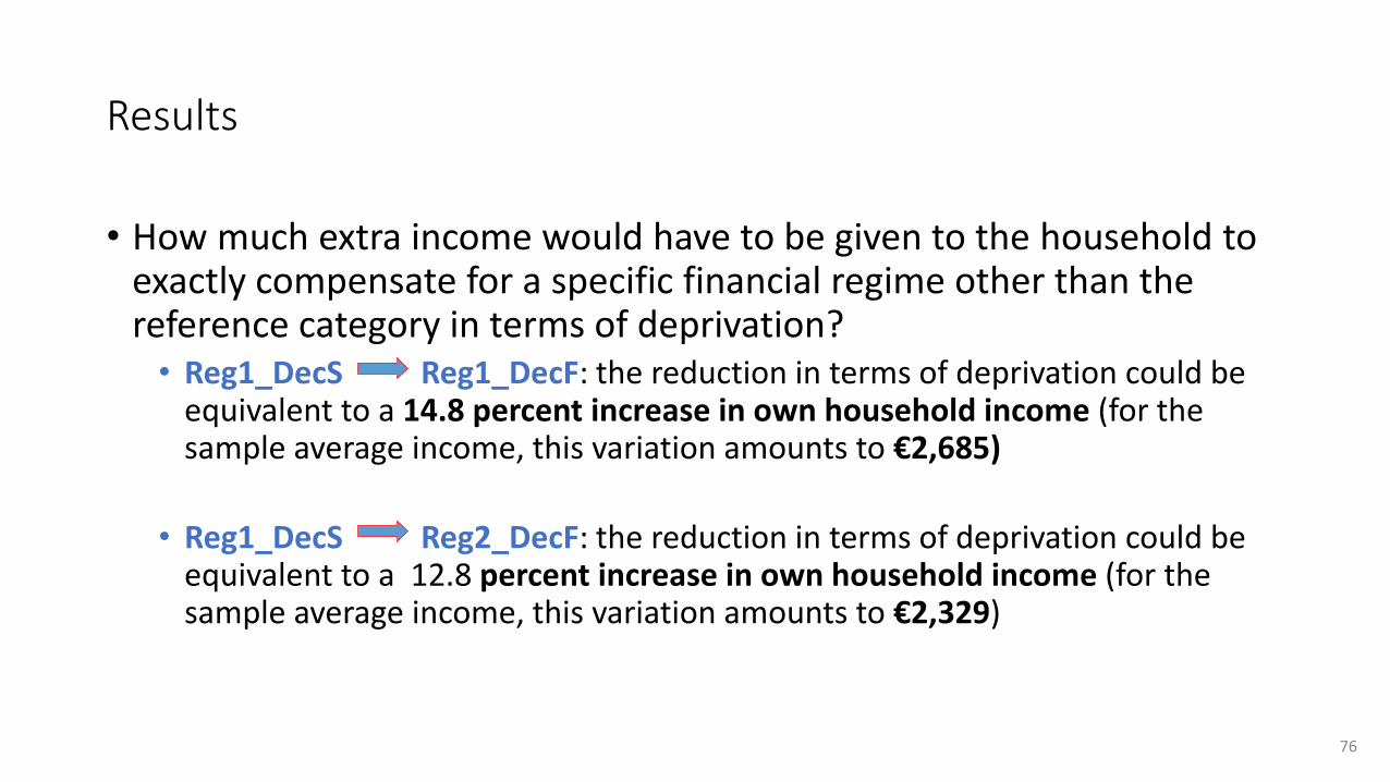
Results

• How much extra income would have to be given to the household to exactly compensate for a specific financial regime other than the reference category in terms of deprivation?

• Reg1_DecS Reg1_DecF: the reduction in terms of deprivation could be equivalent to a 14.8 percent increase in own household income (for the sample average income, this variation amounts to €2,685)

• Reg1_DecS Reg2_DecF: the reduction in terms of deprivation could be equivalent to a 12.8 percent increase in own household income (for the sample average income, this variation amounts to €2,329)

76

Conclusions

• Interesting insight on the role that income pooling and decision making within the household play in determining material deprivation.

• Pooling all incomes and sharing decisions, once controlling for the effects of other socio-economic determinants, is associated with lower levels of deprivation.

• The financial regimen where females have most decision responsibilities is associated with similar low levels of deprivation.

77

Conclusions

• The worst situation in terms of household deprivation is that in which couple members keep part of their incomes separately and decisions are shared.

• Household deprivation level is influenced by what is happening within the household in terms of income pooling and decision making.

• As far as possible, it is crucial to take into account the pooling decisions as well as the decision-making processes and power relations within the family in designing policies to reduce deprivation.

78

Gender inequality, measurement and evidence

Elena Bárcena-Martín

Universidad de Málaga Spain

Winter School on Inequality and Social Welfare Theory

Canazei, January 2018

79

Gender inequality, measurement and evidence

Documents

Transcript of Gender inequality, measurement and evidence