Fuel Quality Issues in Stationary Fuel Cell Systems Quality Issues in Stationary Fuel Cell Systems...

Fuel Quality Issues in Stationary Fuel Cell Systems

ANL/CSE/FCT/FQ-2011-11

Chemical Sciences and Engineering Division

Availability of This ReportThis report is available, at no cost, at http://www.osti.gov/bridge. It is also available on paper to the U.S. Department of Energy and its contractors, for a processing fee, from: U.S. Department of Energy OfficeofScientificandTechnicalInformation P.O. Box 62 Oak Ridge, TN 37831-0062 phone (865) 576-8401 fax (865) 576-5728 [email protected]

DisclaimerThis report was prepared as an account of work sponsored by an agency of the United States Government. Neither the United States Governmentnoranyagencythereof,norUChicagoArgonne,LLC,noranyoftheiremployeesorofficers,makesanywarranty,expressor implied, or assumes any legal liability or responsibility for the accuracy, completeness, or usefulness of any information, apparatus, product,orprocessdisclosed,orrepresentsthatitsusewouldnotinfringeprivatelyownedrights.Referencehereintoanyspecific commercial product, process, or service by trade name, trademark, manufacturer, or otherwise, does not necessarily constitute or imply its endorsement, recommendation, or favoring by the United States Government or any agency thereof. The views and opinions of documentauthorsexpressedhereindonotnecessarilystateorreflectthoseoftheUnitedStatesGovernmentoranyagencythereof,Argonne National Laboratory, or UChicago Argonne, LLC.

About Argonne National Laboratory Argonne is a U.S. Department of Energy laboratory managed by UChicago Argonne, LLC under contract DE-AC02-06CH11357. The Laboratory’s main facility is outside Chicago, at 9700 South Cass Avenue, Argonne, Illinois 60439. For information about Argonne and its pioneering science and technology programs, see www.anl.gov.

Fuel Quality Issues in Stationary Fuel Cell Systems

prepared byD.D. Papadias, S. Ahmed, R. KumarChemical Sciences and Engineering Division, Argonne National Laboratory

November 2011

ANL/CSE/FCT/FQ-2011-11

Table of Contents

1. Introduction ......................................................................................................................................................... 1

2. Biogas resources ................................................................................................................................................. 1

3. Impurities ............................................................................................................................................................ 2 3.1. Sulfur .............................................................................................................................................................. 3 3.2. Siloxanes ......................................................................................................................................................... 4 3.3. Volatile Organic Compounds (VOC) ........................................................................................................... 5

4. Impurity Removal ............................................................................................................................................. 5 4.1. The Process .................................................................................................................................................... 6 4.2. Primary Clean-up (H2S) ............................................................................................................................... 8 Iron oxide design parameters (base case) and assumptions ....................................................................... 10 4.3. Gas drying (Condensation) ......................................................................................................................... 10 Chiller/Condenser design parameters (base case) and assumptions .......................................................... 11 4.4. Low Temperature Polisher (Ordinary Activated Carbon) ...................................................................... 11 4.5. Activated Carbon Effectiveness (ADG) ..................................................................................................... 12 Carbon bed design parameters (base case) and assumptions ..................................................................... 15 4.6. Activated Carbon Effectiveness (LFG) ...................................................................................................... 15 4.7. High Temperature Polisher ........................................................................................................................ 16 High temperature polisher parameters (base case) and assumptions ......................................................... 16

5. Economic Analysis........................................................................................................................................... 16 5.1. Cost Factors and Financial Inputs ............................................................................................................. 16 5.2. Cost of Electricity – Base Case (ADG) ....................................................................................................... 17 5.3. Cost of Electricity – LFG ............................................................................................................................ 19

6. Summary and Conclusions ............................................................................................................................ 21

Acknowledgment .................................................................................................................................................... 21

Acronyms ................................................................................................................................................................ 22

References ................................................................................................................................................................ 22 Appendix 1. Impurity tolerance of AFC, PAFC, MCFC, and SOFC......................................................................... 28 Appendix 2. Frequently occurring trace contaminants for LFG and ADG used for the analysis (excerpt from database) ........................................................................................................................ 30 Appendix 3. Affinity (β) and volume adjusting (kv) coefficients for the Dubinin-Radushkevich (D-R) adsorption isotherm. Coefficients calibrated with experimental data (and specific carbon) were recalculated for BPL (V0=0.42 cm3/g). Correlated isotherms used the reference species as denoted in the parenthesis (species #). ............................................................................................................... 32 Appendix 4. Table A. Financial inputs and cost factor for the fuel cell system ...................................................... 34 Appendix 4. Table B. Capital and maintenance costs for the clean-up system........................................................ 35

P a g e | 1

1. Introduction

Fuel cell systems are being deployed in stationary applications for the generation of electricity, heat, and hydrogen. These systems use a variety of fuel cell types, ranging from the low temperature polymer electrolyte fuel cell (PEFC) to the high temperature solid oxide fuel cell (SOFC). Depending on the application and location, these systems are being designed to operate on reformate or syngas produced from various fuels that include natural gas, biogas, coal gas, etc. All of these fuels contain species that can potentially damage the fuel cell anode or other unit operations and processes that precede the fuel cell stack. These detrimental effects include loss in performance or durability, and attenuating these effects requires additional components to reduce the impurity concentrations to tolerable levels, if not eliminate the impurity entirely. These impurity management components increase the complexity of the fuel cell system, and they add to the system’s capital and operating costs (such as regeneration, replacement and disposal of spent material and maintenance). This project reviewed the public domain information available on the impurities encountered in stationary fuel cell systems, and the effects of the impurities on the fuel cells. A database has been set up that classifies the impurities, especially in renewable fuels, such as landfill gas and anaerobic digester gas. It documents the known deleterious effects on fuel cells, and the maximum allowable concentrations of select impurities suggested by manufacturers and researchers. The literature review helped to identify the impurity removal strategies that are available, and their effectiveness, capacity, and cost. A generic model of a stationary fuel-cell based power plant operating on digester and landfill gas has been developed; it includes a gas processing unit, followed by a fuel cell system. The model includes the key impurity removal steps to enable predictions of impurity breakthrough, component sizing, and utility needs. These data, along with process efficiency results from the model, were subsequently used to calculate the cost of electricity. Sensitivity analyses were conducted to correlate the concentrations of key impurities in the fuel gas feedstock to the cost of electricity.

2. Biogas Resources

Waste-derived fuels are attracting attention as a renewable source of energy, and they are being considered as feedstock for stationary power and CHP systems. General waste streams considered in this report include anaerobic digester gas (ADG) from

wastewater treatment plants and landfill gas (LFG) from municipal solid waste. Landfill gas has been the subject of numerous studies around the world and the U. S. Environmental Protection Agency (EPA) has published a large amount of data that it has collected over the years [1]. Landfill gas is the by-product of the decomposition of organic matter in municipal solid waste (MSW); typical composition of MSW is shown in Figure 1. The total MSW generated in the U.S. in 2009 was 243 million tons, of which, approximately 54% was deposited in landfills [2]. Besides MSW, other wastes may also be landfilled, including construction and demolition debris, wastewater sludge, and non-hazardous industrial waste.

Figure 1. Materials in municipal solid waste (wt%) before recycling. A total of 243 million tons of waste was generated in the US in 2009 [2].

When waste is deposited in a landfill, it undergoes a series of decomposition phases during a period of approximately one year1. Initially, aerobic decomposition takes place where oxygen is consumed forming carbon dioxide, water and heat. Upon oxygen depletion, anaerobic decomposition takes place where the final phase is characterized by a steady production of LFG. This gas is typically saturated with water vapor, and it contains mainly methane (40–60%) and carbon dioxide (35–50%), with smaller amounts of oxygen <1% and nitrogen (3-5%) [3,4]. Generally, one million tons of MSW produce approximately 430,000 standard cubic feet (scf) per day of LFG for 20–30 years after being deposited in the landfill. Of the nearly 2,300 landfills in the U.S., there are currently ~550 operational projects in 40 states that collect landfill gas to produce 1,727 MW of electric power2 and 312

1 http://www.epa.gov/outreach/lmop/publications-tools/handbook.html 2 The majority of power generated by reciprocating engines

P a g e | 2

million scf/day of fuel gas for commercial and residential heating. There are another ~500 candidate sites that could produce an additional 1,170 MW of electricity3. Anaerobic digestion is commonly employed in many wastewater treatment plants (WWTP) to biochemically stabilize the sludge before final treatment and disposal [5,6]. Digesters are most often operated in two temperature ranges, a) mesophilic range (30–37°C) and b) thermophillic range (50–57°C), which primarily affect the decomposition rate and heat addition to the process. The by-product of the decomposition is biogas that has an average methane content of ~60%, with the balance of the biogas consisting primarily of CO2 [6,7]. Typically, approximately 1 scf of biogas is produced per 100 gallons of wastewater treated [7]. The EPA Combined Heat and Power Partnership estimates that energy recovery is not economically feasible for treatment plants with treatment capacities of less than 5 million gallons per day (MGD) [7]. Of the nearly 16,000 publically owned treatment facilities in the U.S., about 1000 treat >5 MGD, as shown in Table 1 [7]. While anaerobic digestion is used for ~60% of the total combined flow for all plants, a significant part of the gas is not utilized. This is especially so for plants with capacities below 75 MGD.

Nearly 4% of the U.S. electrical consumption is used to move and treat water/wastewater [8]. Utilizing the energy content of the ADG can offset part of the WWTPs’ power requirements. Figure 2 shows an example of the offset for the power requirements for activated sludge treatment plants [6]. It plots the energy

3 EPA-Landfill Methane Outreach Program,www.epa.gov/lmop

ratio (the plant’s electrical power demand to the heating value of the ADG4), as a function of the plant’s water treatment capacity. For instance, a 10 MGD plant that consumes 468 kWe and produces a biogas with an energy content of 700 kWth (LHV) has an energy ratio of ~0.67. This can be viewed as the inefficiency of the plant. By using fuel cells to convert the biogas to electricity5, in combination with other plant energy improvements [9], it is possible to recover a substantial fraction of the energy need of the WWTPs.

3. Impurities

Waste-derived fuels contain a variety of trace contaminants, some of which are produced by biological digestion, while others are volatilized from the waste stream being digested. The contaminant

4 Thermal Power calculated (LHV) assumes 60% methane in biogas, and 1 ft3-biogas/100 gallon water treated (70 kWth/MGD) 5 Efficiency of high temperature fuel cell ~45-60%, (www1.eere.energy.gov/hydrogenandfuelcells)

WWTPs by

Flow Rates

(MGD)

Total

WWTPs

Total

wastewater

flow

(MGD)

Wastewater flow

to WWTPs with

ADG

(MGD)

WWTPs with

ADG utilizing

biogas

(%)

Power

wasteda)

(MWth)

>200 15 5,147 3,783 50 159 100 - 200 26 3,885 2,652 53 84 75 – 100 27 2,321 1,350 44 52 50 – 75 30 1,847 1,125 28 56 20 – 50 178 5,375 2,573 29 132 10 – 20 286 3,883 2,039 13 125 5 - 10 504 3,489 1,728 15 103

Total 1,066 25,945 15,247 19 711

a)Power not utilized for WWTPs with ADG. Power calculated assumes 60% methane in biogas, and 1 ft3-biogas generated for every 100 gallon water treated (Power (LHV)=70 kWth/MGD)

Table 1. Capacity and ADG utilization of wastewater treatment plants in the U.S. Influx classified by flow rate [7].

Figure 2. Calculated electrical to thermal power ratio for treatment plants with ADG. Electrical power consumption based on activated sludge treatment plants, excluding building lighting1 .

P a g e | 3

matrix can be rather complex, containing several hundred species that can potentially damage the fuel cell anode6 or other unit operations and processes that precede the fuel cell stack. The amounts and speciation of such trace contaminants depend on various factors, such as the type and age of waste, temperature and pressure, and the stage reached in the decomposition process [3,10–12]. We have reviewed published data with emphasis on the low level impurities present in LFG and ADG and we have set up a database7 that currently includes a total of nearly 300 impurity species found in the biogas matrix. The database classifies the impurities in categories (such as sulfur, siloxanes, halogens, and aromatics) and provides links to specific properties of the species. The database breaks down the information by location, the number of data points on each species, and the minimum, maximum, and average concentrations of the species, as well as information regarding the refuse type, flow-rates, and origin and age of waste. The objective of this task was to compile the data and identify the impurities that can affect the performance of fuel cell systems, and the commonalities between the various biogas matrices. Although a direct comparison for each biogas source would be impractical—as each waste source shows great variability in trace components—it is possible to identify the similarities and differences on an average basis among the various biogas sources. In general, while many contaminant species are present in biogas, three classes of impurities were found to be of particular concern for use of the biogas in fuel cell power (or combined heat and power) systems: sulfur, siloxanes, and volatile organic compounds (VOCs).

3.1. Sulfur

Reduced sulfur compounds are common and often present in significant concentrations in all biogas sources. Most often, sulfur is present as hydrogen sulfide (H2S) at concentrations up to several thousand parts per million by volume. The highest level of sulfur is found in ADG of dairy streams, and there it can range from 500 to 3000 ppm [12]. In comparison to dairy waste, the H2S concentration in biogas produced by wastewater treatment plants is usually smaller, with a range of ~10 to 1200 ppm, as shown in Figure 3. The actual concentrations fluctuate and depend on the liquid sanitary wastes collected and

6 Appendix 1 lists impurity tolerance limits for high temperature fuel cells for some of the impurities of concern (progress report to DOE’s Fuel Cell Technologies Program, November 2010) 7 http://www.cse.anl.gov/FCs_on_biogas

treated, and the specific treatment employed by the facility. For most cases where the concentration of H2S is low, iron salts (such as ferrous chloride) are used in the water treatment process to remove phosphorous and H2S as part of local air quality management [10,13]. High concentrations of H2S (3000 ppm) in WWTP have been reported in the literature [14], where the origin of the high sulfur concentration was found to be the soil through which the untreated water flowed between the source and the destination treatment facility. While H2S contains the bulk of sulfur in the biogas, organic sulfur species such as mercaptans, e.g., dimethyl sulfide (DMS), are also present, although they rarely exceed 0.1 ppm. Typically, LFG contains <100 ppm H2S; however, the concentrations can rise to several thousand ppm in landfills with a high sulfur load. Extremely high concentrations have been measured at landfill cells where large quantities of plasterboard, wastewater sludge, or flue gas desulfurization sludge have been deposited [3]. Just as in ADG, the majority of the sulfur found in LFG is in the form of H2S.

Figure 3. H2S concentration in digester gas from wastewater treatment plants. Excerpt from database.

Figure 4. Concentrations of the most frequent sulfur species measured in landfill gas (LFG). Excerpt from database.

Su

lfu

r s

pe

cie

s in

LF

G (

pp

m)

5400

3.91

0.27 0.34

14.3

0.830.42

62.70

1.34

0.12 0.14

5.55

0.190.13

0.01

0.1

1

10

100

1000

10000Max

Average

P a g e | 4

In contrast to ADG, however, organic sulfur is found in higher concentrations in LFG, usually as mercaptans (thiols), disulphides, and dimethyl sulfide, as shown in Figure 4. In most cases where organic sulfur has been measured at a landfill, dimethyl sulfide was found to be present at concentrations >10 ppm. Organic sulfur species react with hydrogen and carbon oxides, especially at elevated temperatures, to form H2S and COS. Hydrogen sulfide is corrosive to the pipeline infrastructure [15], hence pipes and tubes within the process that are exposed to sulfur need appropriate protection. More importantly, sulfur species deactivate catalysts in the reformer and in the fuel cell anode by reacting with the metals to form sulfides. The acceptable sulfur level in terms of short term degradation can be higher in the case of a fuel cell operating with high concentrations of H2; however, a much lower concentration may be tolerable in fuel cells that reform the fuel internally in the anode [16].

3.2. Siloxanes

Siloxanes are organic silicon compounds typically used in consumer products such as personal hygiene

products, cosmetics, detergents, pharmaceuticals, and lubricants [3,17,18]. Of the hundreds of different siloxanes in use, the most commonly occurring ones in landfill and biogases are the linear species designated with the letter L (L2–L5) and cyclic species designated with the letter D (D3–D6). In comparison to landfill gas, biogas from waste water sludge digestion usually has a higher siloxane concentration, with the majority of those species consisting primarily of D4 and D5, as shown in Figure 5. Landfill gas may contain significant quantities of other siloxanes, such as trimethylsilanol (TMS), as well. The higher siloxane content in ADG may be due to the water solubility of the compounds and also due to the increased volatilization of siloxanes caused by the elevated temperature used in the AD process [3,13,18]. For instance, there seems to be a correlation that siloxane concentrations are higher in thermophilic digesters operating at temperature of about 55°C than in mesophilic digesters operating at 30–35°C [3,13,18]. Siloxanes in the fuel gas can lead to the formation and deposition of SiO2 that can affect many components of the fuel cell system, such as heat exchangers, catalysts, and sensors [3,19,20]. Few studies have investigated

Figure 5. Average concentrations of siloxanes measured in LFG and ADG from wastewater treatment plants. Excerpt from database.

P a g e | 5

the effect of siloxanes on fuel cells. Haga et al. [19] showed that 10 ppm of D5 resulted in total SOFC failure in 30 h at 1000°C. The degradation was almost immediate at 800°C. The cause of the failure was the formation of microcrystalline silica on the anode surfaces.

3.3. Volatile Organic Compounds (VOC)

Waste derived fuels contain species such as alkanes, alcohols, aromatics and halogens. The concentrations of halogens are typically higher in landfill gas than in digester gas from waste water treatment plants, as shown in Figure 6. Landfill gas, for instance, may contain halogenated hydrocarbons from many sources, generally from discarded refrigerants, plastic foams, aerosols, and paints [10]. Many compounds are stable and slowly evaporate to maintain significant high levels of halogens for many years [11]. Chlorine is the most abundant halogen species, while bromine- and fluorine-containing substances are generally found in smaller concentrations. The most commonly occurring fluorine compounds in LFG are chlorofluorocarbons (CFC) used in refrigerants, insulation foams, and propellants [3].

Among hydrocarbons, aromatic and paraffinic hydrocarbons are usually found in high concentrations in LFG, as shown in Figure 7. Such species are encountered in digesters gas as well, but usually at lower concentrations [21]. Among aromatic species, benzene, toluene, and xylene are typically measured at high concentrations. The concentrations of aromatics

are affected by both the age (decomposition process) and the source of the waste [10,11,21]. Toluene, for instance, is commonly used in making paints, lacquers, adhesives, and cosmetic products [21]. While the hydrocarbon concentrations typically found in waste-derived fuels may not be hazardous to the fuel cell, they can greatly reduce the clean-up capacity of various adsorbents for siloxanes [20]. Of primary concern to the fuel cell system are halocarbons, as they convert to acid gas that can corrode catalytic surfaces [22–24]. For Molten Carbonate Fuel Cells (MCFC’s), degradation due to halogens is also a long term effect; halogens react with the electrolyte, thereby affecting the performance of the MCFC over time [23,25].

4. Impurity Removal The specific tolerance of a fuel cell to a given impurity is determined by the nature of the impurity and its interactions with the materials in the anode chamber, which includes the electrocatalyst and the electrolyte. The tolerance limit is defined by considerations of desired lifetime and the end-of-life power output capacity, and the trade-offs between loss in power output against the costs of impurity removal, maintenance, and process reliability. Of the various fuel cell types used in stationary installations, the impurities identified and the data sources for MCFCs are the broadest, since this type of fuel cell has been used in demonstrations using a variety of fuel feedstocks. The data summarized in Appendix 1 provide a glimpse at the levels of individual and class of impurities that may be allowable in the fuel gas fed to the fuel cell anode [3,20,26–37]. There is a wealth of data on the impurity effects for the Polymer Electrolyte Fuel Cell (PEFC), but the open literature reports mostly on automotive PEFCs. The Phosphoric Acid Fuel Cell

Co

ncen

trati

on

(p

pm

)

40.1

0.7

15.6 15.4

3.1

0.8

8.16.8

5.5

0.7

1.5

0.05

0.50

5.00

50.00LFG (Max)

LFG (Average)

ADG (Max)

Figure 6. Examples of typical halogenated species measured in LFG and ADG from wastewater treatment plants. Excerpt from database.

Figure 7. Among the measured non-methane hydrocarbons, aromatic and paraffinic hydrocarbons dominate in LFG. Excerpt from database.

P a g e | 6

(PAFC) has been widely deployed in commercial applications in the US and abroad. The reports on these deployments, however, focus mainly on the application experience and performance, rather than on impurity effects. As the requirements for gas cleaning vary widely from project to project due to the variability in the source fuel gas, the processes have typically been custom engineered for each project. Thus, there are no standard solutions; rather, a specific combination of impurity removal methods is used to ensure a fuel gas of the quality that meets fuel cell tolerance defined by the manufacturer. The published literature [20,38–44] indicates that the gas clean-up strategies involve a primary clean-up, followed by a gas polishing step, before the gas is delivered to the fuel cell system. A generic model of a stationary fuel-cell-based power plant has been developed to assess the overall electrical efficiency and clean-up and maintenance costs determined by the biogas impurity matrix. The system, shown in Figure 8, is detailed in the sections below.

4.1. The Process

As a base case system, we have considered a 300-kWe molten carbonate fuel cell system operated on digester

gas from a waste water treatment plant, which would be applicable for treatment facilities with influent rates of waste water in the order of 10 MGD. The main gas composition of the digester gas (excluding trace impurities) was assumed to be 58% CH4, 38% CO2 and 1% each of O2 and N2 on a dry basis. The gas is also saturated with water vapor at 33°C (reflecting conditions in a mesophilic digester). The concentrations of the trace contaminants used for this analysis are given in Appendix 2 as maximum and average values for both ADG and LFG. Forty-seven species were considered, distributed in 10 classes of contaminants (siloxanes, sulfur, halogens, etc.). Within each class, we included species of most frequent occurrence in the biogas, and also if some contaminants showed particularly high concentrations (based on data from the database). The concentration of some isomers (such as dichlorobenzene, xylene) were added together and grouped into a single species. In cases where the data were too limited to determine average concentrations (as in ADG), the maximum concentration value was used. The main gas processing unit (GPU) of the system is shown in Figure 8. First the bulk impurity, e.g., H2S, is removed using an appropriate technology, such as iron oxide or impregnated carbon. The gas is then cooled to

Figure 8. Process model for a molten carbonate fuel cell system operating on anaerobic digester gas.

P a g e | 7

remove the bulk of water vapor in the gas; and it may even be cooled to below 0°C to condense some of the siloxanes. The gas is then passed to the secondary polishing equipment (low temperature polisher) that can contain a series of adsorbents (i.e. activated carbon, silica, zeolites) that removes organic sulfur, siloxanes, and halogens. The cleaned fuel gas is then fed to the fuel cell module, as shown in Figure 9. The fuel cell module includes a high temperature polisher to remove trace organic sulfur and halogenated species that are not captured by the gas processing unit [44,90,91]. The hydrogen needed for the hydro-desulfurizing unit (HDS) is obtained from the anode tail-gas, recycling 6% of it back to the inlet fuel. This anode slip-stream is cooled to 60°C, to condense out the bulk of the water and increase the hydrogen concentration, before it is mixed with the fuel from the GPU. The fuel gas mixture is compressed to ~25 psia and heated to 330°C before entering the high temperature polisher. The cleaned gas is mixed with steam (steam-to-carbon ratio of 2.5) and fed to a pre-reformer, where the fuel is partially reformed at a temperature of 440°C before entering the fuel cell stack.

For the fuel cell, we have used a model similar to that developed by Lukas et al. [45]. The model discretizes the stack into 40 well stirred control volumes for both the anode and cathode, and it assumes that the temperature is equal within each control volume. The model accounts for the internal reforming reactions and fuel cell irreversible losses contributed by activation, concentration, and ohmic polarizations [45,46]. The partially reformed fuel enters the anode where it is further internally reformed via methane steam reforming (SMR) (Eq. 1) and the water gas shift reaction (WGS, Eq. 2) to hydrogen. The hydrogen reacts by the anode half-cell electrochemical reaction (Eq. 3). For the SMR reaction, we used the kinetics used by Lukas et al. [46]. It was assumed that the WGS reaction is equilibrium limited. Only hydrogen participates in the electrochemical reaction. Methane Steam Reforming

�� 2��⇔ �� 3�� (1)

Figure 9. The fuel cell module includes the stack (300 kW MCFC), balance of plant (BOP), and high temperature polisher.

P a g e | 8

Water Gas shift

�� ⇔ �� (2) Anode half-cell electrochemical reaction

�� ⇒�� 2 � (3) The anode tail gas is fed to the burner and recycled to the cathode where the following electrochemical reaction takes place, Cathode half-cell electrochemical reaction

�� 2 � ⇒ �� (4)

The cathode effluent, after passing a series of heat exchangers (i.e. for anode gas pre-heating, steam generation), enters the heat recovery unit at ~380°C (~710°F) and leaves the system as waste heat at 110°C. The recovered heat can be used by the water treatment plant to meet the energy needs for the anaerobic digestion process and, if possible, for space heating. Given the assumptions for the process shown in Table 2, a net electrical efficiency of 47% and a total efficiency of 69.5% based on the fuel (biogas) LHV was calculated. This value corresponds closely to the efficiencies reported for MCFC demonstration projects operated on anaerobic digester gas and in the manufacturer’s data [47]. The following sections discuss the fuel gas clean-up steps in more detail.

4.2. Primary Clean-up (H2S)

In our base case system, we have chosen to use an iron oxide media, SulfaTreatHP®, as the means to remove hydrogen sulfide as the first step in the clean-up sequence in the GPU. There are many other choices to remove H2S, such as impregnated activated carbon [48–51], and other proprietary iron oxide media, such as Sulfur-Rite®, Sulfa-Bind®, and Iron Sponge, as well. The manufacturer of the particular media often states a maximum adsorption capacity that is equivalent to saturation conditions (i.e., the concentration in the exit gas equals the concentration in the feed gas). Actual breakthrough data and the adsorption capacity as a function of the exit concentration were not available. Part of the reason for choosing this iron oxide media was that pieces of information regarding the use of

Table 2. Operating conditions and system efficiencies for MCFC plant

Characteristics Value Units

Fuel Cell Fuel Utilization 70 % Oxygen utilization 40 % Voltage 767 mV Current density 137 mA/cm2 DC/AC efficiency 98 % Pressure 137 kPa Balance of Plant Parasitic power (GPU+Fuel Cell plant)

22.3 kW

Compressor/blower efficiency

78 %

Heat loss – Heat exchanger 8 % of heat load

Heat loss – Burner 10 % of anode LHV

Heat loss – Fuel Cell 1.8 % of fuel LHV Efficiencies Net electrical efficiency 47 % of fuel LHV Total CHP efficiency 69.5 % of fuel LHV

SulfaTreat® in case studies [44,47] and in the literature [52] were helpful in developing a model for design purposes. The model considers the transient behavior of a packed bed filled with spherical particles. It is a two-phase model accounting for the gas phase as well as the solid phase. It also includes axial mass dispersion in the gas phase. The equation for the particle assumes that diffusion is the rate limiting process, and it is derived from the principles of the shrinking core model [53,54]. The model could be fitted to the breakthrough data of Truong et al [52] (see Figure 10), and it could also predict the effects of other experimental conditions (e.g., varying flow rates and H2S concentrations). However, the experiments were done at room temperature and, at such conditions, iron oxide media perform poorly (only 2.8 wt% adsorption capacity of sulfur was achieved, as opposed to a maximum of ~12 wt%). In tests done at the Anoka Landfill with SulfaTreat®, low temperatures (below 38°C) were the cause of early breakthrough of H2S; once the bed was heated, the H2S dropped to levels below the detection limit (100 ppb). Unfortunately, the size of the beds was not disclosed in that report [44]; however, the information was useful in that the operating parameters (temperature) were shown to be very important in achieving a high adsorption capacity. Furthermore, while the inlet concentration of H2S varied between 60 and 100 ppm, the iron oxide media effectively reduced the exit gas content to below 0.1 ppm (detection limit).

P a g e | 9

Methyl mercaptan was removed completely as well, corroborating information from the manufacturer that the iron oxide media is effective for the removal of mercaptans. The iron oxide media was ineffective in removing dimethyl sulfide (DMS), however [44]. The model was calibrated with the data from the King County Case Study, using breakthrough times projected by the vendor from the flows and bed sizes used in the process [47]. Figure 11 shows the adsorbent utilization as a function of contact time (or residence time) of the gas in the bed, with kinetics evaluated based on the King County Case Study8. A frequently stated residence time for effective performance appears to be in the order of ~60–120 s [55]. This is approximately what we observe in Figure 11. As the contact time increases, there is a positive effect on the utilization of the sorbent (especially in the range of 30–120 s). Above ~120 s, however, sorbent utilization is not as effective. The increase in the utilization of the adsorbent becomes less effective at contact times above ~120 s. This is an effect that gas-phase transport phenomena become important at high contact times. To maintain a constant pressure drop as the bed volume increases, the diameter of the bed increases but doing so, the velocity in the bed is decreased. The lower velocities in the bed reduces the mass transfer rates of i.e. H2S from the gas phase to the solid and also increases the magnitude of axial dispersion in the bed. The “breakthrough concentration” is defined as the concentration of the impurity in the bed effluent when the bed is considered to have reached its capacity. This value is usually a percentage of the inlet concentration of the species, and it is selected by the design engineer.

8 Kinetics were increased by a factor of 4 (to 4x10-8 m2/s) in comparison to the data by Truong et al. [40]

Defining a higher breakthrough concentration of H2S allows greater utilization of the sulfur sorption capacity. If only one vessel is used (and no other means to remove H2S are used after this treatment step) assigning a low breakthrough concentration (e.g., 0.1 ppm) would underutilize the sorbent. It is common to have two vessels operated in series (called lead and lag configuration). When the lead vessel reaches the breakthrough concentration the flow is switched to make the second vessel the lead vessel, while the lag vessel is refilled with fresh media and made the new lag vessel. This lead and lag configuration can be viewed as a safety net to account for variations in operating conditions (such as temperature and the inlet concentration of the contaminant).

0 20 40 60 80 1000

100

200

300

400

500

600

700

Symbols represent repeated experimentsunder same operating conditions but with

new batch of SulfaTreat

H2S

bre

akt

hro

ugh

co

nce

ntr

atio

n (

ppm

)

Time (hours)

Model

Experiments on Sulfatreat1

• H2S inlet Conc. : 3000 ppm• Rated Flow: 20 L/hr• CO2 29 %• CH4 61 %

• Relative humidity: 100 %

• Temperature: 293 K• Bed contact time: 60 s• Bed diameter: 6.35 cm

Assumptions: Particle diameter: 0.5 cmBed density: 1 g/cm3

Max H2S capacity: 12 wt-%Diffusivity (kinetics): De=1x10-8 m2/s

Figure 10. Comparison between modeled and experimental breakthrough concentrations of H2S on Sulfatreat.

0

0.02

0.04

0.06

0.08

0.1

0.12

0 20 40 60 80 100 120 140 160 180

Uti

lizati

on

(g

-S/g

-Ad

so

rben

t)

10 ppm breakthrough

0.1 ppm breakthrough

Contact time (s)

Inlet H2S concentration to bed: 1000 ppm

Bed volume increases

Figure 11. Calculated sulfur capacity on iron oxide media as a function of contact time and breakthrough concentration of H2S. Maximum sulfur capacity of media assumes 0.12 g-S/g-adsorbent. Vessel length over diameter ratio (L/D)=2.

P a g e | 10

A lead and lag configuration may increase the utilization of the adsorbent by up to 20% in comparison to a single vessel operation9. Iron oxide design parameters (base case) and

assumptions

• Contact time: 120 s

• 2 vessel design (equal bed volumes), lead and lag configuration

• Lead vessel breakthrough concentration of H2S: 15 ppm

• Temperature: 38°C

• H2S and mercaptans removed: All other organic sulfur is assumed to break through continuously

4.3. Gas drying (by Cooling/Condensation) The gas needs to be dried before it enters the polisher. Moisture, especially at relative humidities (RH) exceeding 40%, can significantly reduce the capacity of adsorbents, such as activated carbon [56–60]. Some other adsorbents, for example silica gel and zeolites, are extremely sensitive to moisture and may require the gas to be almost dry (RH<10%) [20,61]. For our base case, we consider activated carbon as adsorbent media (section 4.4) and have assumed that an RH of <25% has a negligible effect on the adsorption capacity of the

9www.slb.com/~/media/Files/miswaco/brochures/sulfatreat_10881.ashx

sorbent. After the bulk sulfur removal, the gas is passed to a chiller/condenser that cools the gas to a dew point of 4°C. After removal of the condensed water in a knock- out tank, the gas is reheated to 25°C (RH=25%) via a heat-exchanger by using the warm biogas stream exiting the H2S removal bed (Figure 8). The refrigeration cycle was calculated using the software Duprex 3.2 with Suva™ 134a as the refrigerant10. At a temperature of 4°C, only water was condensed out and all other trace impurities remained in the gas phase (based on vapor pressure), even in cases where the maximum concentration values were used (both for LFG and ADG). Some removal of VOC’s after condensing out the water has been observed in some cases [61]. This may reflect that upon condensation, some soluble species, such as alcohols, may be washed out with the water condensate. However, vapor pressure alone is not enough to predict any condensation of higher hydrocarbons in the concentration range found in the biogas matrix (even after cooling to below 0°C). The only species that were predicted to condense out by vapor pressure alone are cyclic siloxanes, especially D5 [62], Figure 12. Figure 12 shows the effect of temperature and pressure on the condensation efficiency for D5. For low concentrations (1 ppm) and pressures (1 atm),

10 Software available for download by DuPont Refrigerants www.isceon.com/duprex

Figure 12. Theoretical condensation efficiency for D5 (decamethylcyclopentasiloxane) as function of temperature and partial pressure (concentration, pressure).Assumes ideal gas, saturated vapor pressure obtained from AspenPlus®

P a g e | 11

condensation of D5 would start at temperatures below -35°C. At this temperature, if the concentration of D5 is 10 ppm, almost 90% would be removed. Increasing the pressure increases the condensation temperature; for example, at 5 atm and for inlet concentration of 10 ppm, the condensation would start at ~2°C and 90%

could be removed at −20°C. While chilling to below 0°C in combination with high pressures can be effective for some siloxanes, linear siloxanes (such as L2) having higher vapor pressure are likely to remain in the gas phase at high concentrations even after chilling [62]. Furthermore, the requirement of low temperatures and high pressures add to capital cost and increased power consumption, and such a strategy may be advisable only in cases with extremely high concentrations of siloxanes (in particular D5). In our base case, considering that the typical values of D5 are in the range of 1–5 ppm (average concentration of 1.7 ppm), the gas was only dried, with all trace impurities removed in subsequent steps.

Chiller/Condenser design parameters (base case) and

assumptions

• Dew Point: 4°C

• RH at 25°C: 25%

• No trace impurities are condensed/washed out

• Coefficient of performance for refrigeration cycle (COP): 3.4

4.4. Low Temperature Polisher (Activated

Carbon) Activated Carbon (AC) is frequently used for the removal of organic vapors [63–65], and it has also been demonstrated to be efficient in removing siloxanes [61,66]. By AC we define carbon that has not been impregnated (such as KOH-impregnated carbon) or functionalized by, for example, Cu or Cr. Impregnated or functionalized carbons are used to target specific impurities such as H2S or organic sulfur. In this analysis, H2S is removed using an iron oxide bed (Section 4.2), and AC is considered for the first step of the polisher to estimate the effectiveness for removing the trace contaminant matrix as given in Appendix 2. The service life of the carbon depends on the operating parameters (such as temperature and pressure) and by the adsorption affinity of the carbon for the individual species. To properly address the adsorption capacity and the corresponding operating costs of the carbon bed, adsorption data are needed as a function of concentration and temperature for each contaminant species of interest. Furthermore, the adsorption capacity for each adsorbate is greatly influenced by the

other species in the mixture. Aromatic compounds, for instance, will strongly adsorb on carbon and displace many halogenated compounds and siloxanes, leading to an early breakthrough of such species. Therefore, the composition of the mixture is of importance in determining the service life of the bed. The model includes all those effects to estimate the breakthrough for each species in a bed filled with activated carbon. The model is outlined below. Adsorption Isotherms

The Dubinin-Radushkevich (D-R) equation [65] was used to determine the adsorption isotherms for all species given in Appendix 2. We have used the correlation proposed by Ye et al [67]:

�� /��

� (5)

�� !�" (6)

where q = Adsorption capacity (mol-adsorbate/g-carbon) V0 = Active adsorption space (micropore volume of carbon) (cm3/g) Vb = Molar volume of the adsorbate at its normal boiling point (cm3/mol) P = Partial pressure of adsorbate in the gas-phase (atm) Pv = Vapor pressure of adsorbate (atm) T = Temperature (K) β = Affinity coefficient (-) kv = Volume adjusting coefficient (-) Some of the parameters can be readily obtained; Pv, Vb can be obtained from thermodynamic properties [68], and V0 from the carbon manufacturer or by measurement. The affinity coefficient (β) and the pore volume adjusting coefficient (kv) are parameters that need to be estimated [64,65,67,69] or fitted to adsorption isotherm data. For the most part, we could find literature data for many of the species shown in

Appendix 2 and fit equation (5) to those data [50,59,60, 67,69–84]. For the cases where data were not available (8 species), the parameters were correlated by using a reference species of similar properties and the method developed by Ye et al. [67]. The set of coefficients (β and kv) to model the isotherm with eq. (5) are given in Appendix 3. Figure 13 shows the adsorption capacity of activated carbon on some select impurities. The lines are modeled adsorption isotherms on pure organic

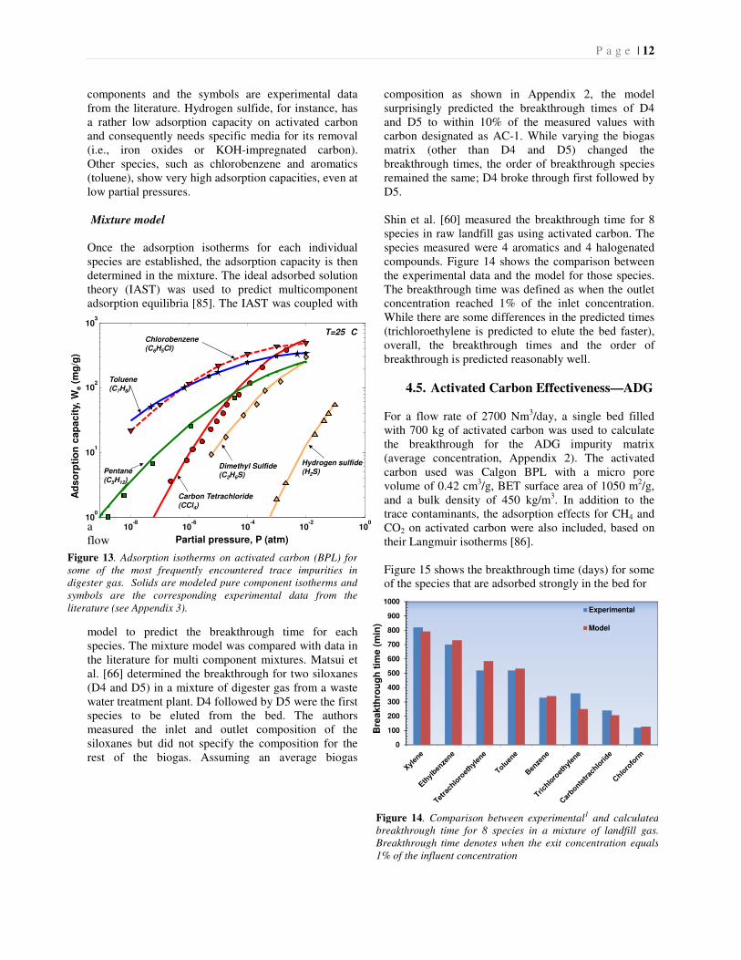
P a g e | 12

components and the symbols are experimental data from the literature. Hydrogen sulfide, for instance, has a rather low adsorption capacity on activated carbon and consequently needs specific media for its removal (i.e., iron oxides or KOH-impregnated carbon). Other species, such as chlorobenzene and aromatics (toluene), show very high adsorption capacities, even at low partial pressures. Mixture model

Once the adsorption isotherms for each individual species are established, the adsorption capacity is then determined in the mixture. The ideal adsorbed solution theory (IAST) was used to predict multicomponent adsorption equilibria [85]. The IAST was coupled with

a flow

model to predict the breakthrough time for each species. The mixture model was compared with data in the literature for multi component mixtures. Matsui et al. [66] determined the breakthrough for two siloxanes (D4 and D5) in a mixture of digester gas from a waste water treatment plant. D4 followed by D5 were the first species to be eluted from the bed. The authors measured the inlet and outlet composition of the siloxanes but did not specify the composition for the rest of the biogas. Assuming an average biogas

composition as shown in Appendix 2, the model surprisingly predicted the breakthrough times of D4 and D5 to within 10% of the measured values with carbon designated as AC-1. While varying the biogas matrix (other than D4 and D5) changed the breakthrough times, the order of breakthrough species remained the same; D4 broke through first followed by D5. Shin et al. [60] measured the breakthrough time for 8 species in raw landfill gas using activated carbon. The species measured were 4 aromatics and 4 halogenated compounds. Figure 14 shows the comparison between the experimental data and the model for those species. The breakthrough time was defined as when the outlet concentration reached 1% of the inlet concentration. While there are some differences in the predicted times (trichloroethylene is predicted to elute the bed faster), overall, the breakthrough times and the order of breakthrough is predicted reasonably well.

4.5. Activated Carbon Effectiveness—ADG For a flow rate of 2700 Nm3/day, a single bed filled with 700 kg of activated carbon was used to calculate the breakthrough for the ADG impurity matrix (average concentration, Appendix 2). The activated carbon used was Calgon BPL with a micro pore volume of 0.42 cm3/g, BET surface area of 1050 m2/g, and a bulk density of 450 kg/m3. In addition to the trace contaminants, the adsorption effects for CH4 and CO2 on activated carbon were also included, based on their Langmuir isotherms [86]. Figure 15 shows the breakthrough time (days) for some of the species that are adsorbed strongly in the bed for

10-8

10-6

10-4

10-2

100

100

101

102

103

Hydrogen sulfide

(H2S)Dimethyl Sulfide(C2H6S)

Carbon Tetrachloride

(CCl4)

Chlorobenzene

(C6H5Cl)

Pentane

(C5H12)

Toluene

(C7H8)

Ad

so

rpti

on

cap

acit

y, W

e(m

g/g

)

Partial pressure, P (atm)

T=25 C

Figure 13. Adsorption isotherms on activated carbon (BPL) forsome of the most frequently encountered trace impurities in digester gas. Solids are modeled pure component isotherms and symbols are the corresponding experimental data from the literature (see Appendix 3).

0

100

200

300

400

500

600

700

800

900

1000Experimental

Model

Bre

akth

rou

gh

tim

e (

min

)

Figure 14. Comparison between experimental1 and calculated breakthrough time for 8 species in a mixture of landfill gas. Breakthrough time denotes when the exit concentration equals 1% of the influent concentration

P a g e | 13

the ADG composition. The value in parentheses after each species denotes the inlet concentration in ppm. Most of those species are aromatics, terpenes (limonene), and high molecular weight hydrocarbons, such as nonane and octane. However, some halogenated species (e.g., dichlorobenzene) and linear siloxanes (e.g., L2) appear to have a strong adsorption affinity on carbon. Figure 16 shows the other side of the species spectrum -species that breakthrough early. Most low molecular weight hydrocarbons, such as ethane and propane, do not adsorb well on carbon and

break through the bed almost immediately. Species of concern to the fuel cell that leave the bed very early (~5 days) are dimethyl sulfide and methylene chloride. The next group of species with early breakthrough are vinyl chloride < carbon disulfide < trichloro-fluormethane, with an estimated breakthrough time of about 30 days. The first siloxane species that was observed to elute the bed is D4 with an approximate breakthrough time of 165 days, followed by D5 (173 days). Since siloxanes are of particular concern for fuel cell systems [3,19,20], a reasonable replacement period for the carbon would be either

before dichloroethane breaks through (81 days) or just before the first siloxane, D4, breaks through (~165 days). Dichloroethane adds ~50% out of the total chlorine concentration (370 ppb), if that species is not captured by the bed (note that there are 2 chlorine atoms per molecule). The total concentration for the chlorine added by dichlorethane is, however, too small to justify more frequent carbon media replacement (81 days as opposed to 165 days for D4).

847

641

467

0 100 200 300 400 500 600 700 800 900

Limonene (9.7 ppm)

Cymene (1.2 ppm)

Nonane (1.3 ppm)

Trimethylbenzene (1.9 ppm)

Xylenes (0.8 ppm)

Ethylbenzene (1.3 ppm)

Octane (0.2 ppm)

1,4-Dichlorobenzene (0.25 ppm)

Heptane (0.36)

(L2) Hexamethyldisiloxane (0.17 ppm)

Tetrachloroethylene (0.1 ppm)

Toluene (1.1 ppm)

Chlorobenzene (0.26 ppm)

Days before breakthrough

Halogens

Hydrocarbons

Siloxanes

Figure 15. Breakthrough time for strongly adsorbed species on activated carbon (average ADG composition). L3 was predicted to adsorb more strongly than L2 and it was not included in the analysis (the concentration of L3 was added to L2).

165

81

31

1

0 20 40 60 80 100 120 140 160 180 200

Hexane (25 ppm ppm)

(D5) Decamethylcyclopentasiloxane (1.7 ppm)

Benzene (0.17)

(D4) Octamethylcyclotetrasiloxane (0.83 ppm)

2-methoxy-2-methyl-propane (MTBE) (0.8 ppm)

Pentane (7 ppm)

1,2-Dichloroethane (0.16 ppm)

Trichlorofluoromethane/R-11 (0.04 ppm)

Carbon Disulfide (0.05 ppm)

Butane (0.7 ppm)

Vinyl Chloride (0.12 ppm)

Methylene Chloride (0.05 ppm)

Dimethyl Sulfide (0.04 ppm)

Propane (1 ppm)

Ethane (40 ppm)Sulfur (as S) (0.14 ppm)- Dimethyl Sulfide- Carbon DisulfideHalogens as Cl (0.69 ppm)- Methylene Chloride

- Vinyl Chloride- Trichlorofluoromethane- Dichloroethane


Halogens

Siloxanes

Oxygenates

Sulfur

Figure 16. Breakthrough times for weakly adsorbed species on activated carbon (average ADG composition).

P a g e | 14

The replacement period for the carbon bed was based on D4 capture (limiting species for the media). This service life of ~165 days will also be influenced by operating parameters and variations in ADG composition. The sensitivity of some of those parameters to the service life of the media is shown in Figures 17a-b. By increasing the pressure, the breakthrough time for D4 decreases. This seems counterintuitive at first, since the adsorption capacity increases with partial pressure (see isotherms in Figure 13). This is true for some species; particularly if their adsorption capacity increases steeply with pressure. However, the other effect of pressure is that it also increases the competition of adsorption space, in particular due to CH4 and CO2. Activated carbon is used in pressure swing adsorption (PSA) to separate those species for hydrogen purification [87]. While CO2 and CH4 do not adsorb on carbon as strongly as VOC, the combination of high concentrations and high pressure will favor their adsorption on the carbon and, thus, reduce the ability of the bed to trap D4. Temperature is an important operating parameter and strongly affects the adsorption capacity for all species. Decreasing the temperature to 10°C will increase the service life of the bed, provided that the relative humidity remains low. However, if the chiller operates at a dew point of 4 °C (base case) the relative humidity will be 66% and this will greatly increase the adsorption of water vapor on the carbon [57,58]. The benefit (higher adsorption capacity for the VOCs and siloxanes) of lower temperature operation is realizable only if the moisture content is lowered before the carbon bed. To gain this benefit will require a different drying strategy, such as chilling below 0°C or using drying media (e.g., silica). This will likely increase the complexity and cost of the system. On a final note, the proper weatherization is important for the carbon beds, especially when operating in colder climates. The bed operating temperature needs to be maintained at or above 25°C to avoid moisture adsorption and even condensation of water in the beds. The concentration of the halogens in ADG is low, and the majority of those species adsorb less strongly than D4. Hence, variations in the concentrations of halogens have little effect on the breakthrough time for D4. On the other hand, variation of concentrations of other

contaminant groups has greater impact on breakthrough times. Among the alkanes, hexane has the greatest effect on the adsorption capacity for D4 (Figure 17b), whereas other alkanes, such as ethane or propane, that have negligible adsorption affinity for carbon, do not affect the breakthrough time for D4. Increasing the concentration of siloxanes increases the replacement frequency for the bed. When the concentration of D4 is increased to 5 ppm (~7 times the base case concentration), the breakthrough time is reduced by 13% to 142 days. For average and moderately high siloxane concentrations, activated carbonappears to be effective for the adsorption of siloxane without the need for deep chilling.

50 70 90 110 130 150 170 190 210 230 250

Alkanes (ppm) (150 -75 - 37)

Aromatic/Cyclic (ppm) (32 - 16 - 8)

Siloxanes (ppm) (1.3 - 2.6 - 5.3)

Temperature (°C) (40 - 25 - 10)

Days before D4 breakthrough

(2)Pressure (atm)

Temperature ( C)

Halogens (ppm)

Siloxanes (ppm)

Aromatic/Cyclic (ppm)

(1.1)

(10)

(0.4)

(40)

Alkanes (ppm)

(1.3)

(2.6)

(25)

(2.6)

(16)

(75)

(150) (37)

(32) (18)

(5.3)(1.3)

a)

50 70 90 110 130 150 170 190 210 230 250

Days before D4 breakthrough

D4 (ppm)

D5 (ppm)

Hexane (ppm)

Limonene (ppm)

Aromatic/Cyclic (ppm)

(0.8)

(0)(5)

Alkanes (ppm)

(1.7)

(5)

(16)

(32) (8)

(35)

(10)

(0)

(75)

(150) (37)

(25)

(50) (12)

b)

Figure 17a-b. Sensitivity of D4 breakthrough time to operating parameters and concentration. The concentration for each species within a class of impurities (e.g., halogens) was either doubled or reduced by half from the average ADG composition.

P a g e | 15

Carbon bed design parameters (base case) and

assumptions

• Pressure: 1.1atm


• Moisture at RH=25% does not affect the adsorption capacity of OAC

• Carbon media: Calgon BPL (700 kg per bed/ 2 beds in series in lead and lag configuration)

• Bed replacement: ~165 days (D4 is the limiting species)

4.6. Activated Carbon Effectiveness—LFG For comparison, the service life of the carbon beds was calculated for the average landfill gas (LFG) composition (Appendix 2). The gas contained 50% CH4, 48% CO2, and 1% each of O2 and N2 on a dry basis. Figure 18 shows the breakthrough times for the species that have the lowest adsorption capacity.

Similar to the ADG case, D411 is the first siloxane to break through. However, due to adsorption competition, in particular due to the higher concentration of hydrocarbons in landfill gas, the breakthrough time for D4 is reduced to 122 days. The concentration of halogens and sulfur that breakthrough before D4 is substantially higher in LFG than ADG. After 5 days of operation, DMS alone accounts for the majority of sulfur (5.6 ppm) and methylene chloride for 12.1 ppm of chlorine (~40% of the total chlorine in LFG). Basing the service life of the carbon beds before D4 breaks through (~122 days), the total chlorine concentration would add up to ~18 ppm. Completing the model calculations for the fuel cell system, the overall and electrical efficiencies were found to be ~70% and 47%, respectively (compared to ~70% and 46% with ADG, see Section 4.1).

11 Landfill gas may contain high concentrations of trimethylsilanol (TMS). Adsorption data for TMS were not found in the literature, however. The properties for TMS were significantly different from those for other siloxane species. We had no confidence to correlate the adsorption isotherm of TMS to those species (reference species)

137

125

122

63

29

5

0

0 20 40 60 80 100 120 140 160

Chlorobenzene (0.55 ppm)

Hexane (3 ppm)

(D5) Decamethylcyclopentasiloxane (0.05 ppm)

Trichloroethylene (0.8 ppm)

Benzene (2 ppm)

1,1,2-Trichloroethane (0.2 ppm)

(D4) Octamethylcyclotetrasiloxane (0.25 ppm)

Carbon Tetrachloride (0.04 ppm)

Pentane (3.2 ppm)

2-Propanol (1.92 ppm)

Chloroform (0.07 ppm)

1,2-Dichloroethane (1.8 ppm)

Acetone (6.8 ppm)

Trichlorofluoromethane/R-11 (0.2 ppm)

Carbon Disulfide (0.14 ppm)

Ethanol (0.22 ppm)

Butane (4.3 ppm)

Vinyl chloride (1.23 ppm)

Methylene Chloride (5.15 ppm)

Dimethyl Sulfide (5.6 ppm)

Propane (12 ppm)

Chlorodifluoromethane/R-22 (0.6 ppm)

Ethane (8.9 ppm)

Halogens

Hydrocarbons

Siloxanes

Oxygenates

Sulfur


S: 5.6 ppmCl: 12.1 ppm

S: 5.9 ppm

Cl: 14.1 ppm

S: 5.9 ppmCl: 18 ppm

Figure 18. Breakthrough times for weakly adsorbed species on activated carbon (average LFG composition).

P a g e | 16

4.7. High Temperature Polisher

For a service life of OAC determined by D4, most of the organic sulfur and some halogenated species will not be adsorbed by the bed. In the case of ADG, where the concentrations of the organic sulfur and halogens are relatively low, if the fuel cell can tolerate these low levels and the raw ADG is not prone to sudden spikes in these species, the gas can be fed directly to the fuel cell. With LFG, however, where the dimethyl sulfide (DMS) and methylene chloride add up to 6 ppm of sulfur and 12 ppm of chlorine (on average), an activated carbon guard bed is highly desirable. Finding effective methods to remove DMS and, in particular, halogens, such as methylene chloride and vinyl chloride, at close to ambient temperatures proved difficult with published technology. For DMS, there are few adsorbents such as Cu-impregnated carbons and zeolites (Zeolite 13X) that can achieve adsorption capacities for sulfur of ~2.5 wt% [88,89]. Such performance most often is for natural gas compositions, and little is known about how biogas will affect the sorption capacity for sulfur. Furthermore, water and CO2 are strongly adsorbed on zeolites and, therefore, the gas to be treated needs to be free of moisture [20]. Data on adsorption of halogens on carbon only confirmed the results in our study that vinyl chloride and, in particular, low molecular weight halogens, such as chloromethane and chloroethane, are poorly adsorbed on many types of activated carbon [44,60,77,89,90]. In the system studied here, all sulfur and chlorinated species not captured by the carbon bed are removed by the high temperature polisher. Such a clean-up process has been used to treat biogas in several case studies for fuel cell systems [44,90,91]. Organic sulfur and chlorine are first reacted with hydrogen over a hydroprocessing catalyst (HDS) (such as Ni-Mo or Co-Mo supported on alumina) and converted to H2S and HCl, respectively. These species are then removed by using sulfur and chlorine adsorbents (i.e., ZnO-based sorbents for H2S, and Al2O3 with metal oxides for chlorine). Screening tests done with 500 ppm of H2S and HCl each over commercial adsorbents12 indicated a removal capacity of ~8–10 wt% for sulfur and chlorine, each, before breakthrough [92]. The tests were conducted at 270–350°C and ambient pressure. The effectiveness of the hydroprocessing catalyst depends on the partial pressure of hydrogen, temperature, and the concentrations of the trace

12G-72E sorbent for H2S and removal and G-92C sorbent for HCl

impurities. He et al. [91] observed good activity for the hydroprocessing catalyst with tests using simulated landfill gas (~150 ppm halogens, and 25 ppm DMS and COS each) operating at 340°C and using a hydrogen partial pressure of ~5 kPa. Oxygen in the gas (1%) and even moisture showed no noticeable effect on the activity of the catalysts and subsequent sorbents.

High temperature polisher parameters (base case)

and assumptions


• H2 partial pressure for HDS: 5 kPa

• Sulfur removal media: G-72E (5 wt% sulfur capacity before breakthrough)

• Chlorine removal media: G-92C (5 wt% chlorine capacity before breakthrough)

• Dual beds for adsorbents for continued operation during media replacement

5. Economic Analysis

5.1. Cost Factors and Financial Inputs Along with the cost factors that impact the economics of the plant, the analysis evaluated the sensitivity of the cost of electricity to the impurity levels in the biogas. Cost factors included in the analysis were

a) Capital costs for the clean-up process and fuel cell system (including stack replacement)

b) Variable costs for maintenance and replacement of spent media

Analytical costs (i.e. grab sampling of the biogas), or any incentives or energy tax credits were not included in this analysis. Cost data were obtained from the published literature [43,48,55,63,92–101]. The capital costs for the iron oxide and the activated carbon vessels are shown in Figure 19 and 20, respectively13. The capital cost for iron oxide beds increases linearly with vessel size, suggesting specialized beds and custom engineering for each project. In contrast, the capital cost for the carbon beds shows some economies of scale, possibly because of wide applications and sizes of such beds for VOC control. Chiller capital costs (excluding compressor/blowers) are $500–700 per scfm for flow rates above 35 scfm [95,101]. For small flow rates, the chillers can cost up to $3000 per scfm, as those units are overdesigned in relation to the flow capacity

13 The cost includes piping and instrumentation and assumes that 2 vessels are used in series

P a g e | 17

[43,101]. For the high-temperature polisher, we have used the system costs estimated by Directed Technologies Inc. (currently Strategic Analysis, Inc) for natural gas polishing14. The cost includes piping and vessels (2 in parallel), and also includes a heat exchanger and HDS catalyst. Cost for the sorption media reflects disposal/regeneration services.

a) The cost for carbon onsite replacement services is reported to be $4–5 per kg or virgin activated carbon, approximately twice the cost of the media ($2/kg) [63,94].

b) The cost for the iron oxide media (Sulfatreat) is reported to be ~$1/kg [48,55,96]. Disposal costs are estimated to be 25–100% of the media cost [97].

c) Sulfur removal media (G-72E) cost: $8.8/kg [92].

d) Chlorine removal media (G-92C) cost: $2.2/kg [92].

Disposal costs for the high temperature polisher media were not reported. Considering that disposal/ regeneration may cost as much as the media itself, we have assumed that all replacement costs equal the cost of the media. Tables A and B in Appendix 4 summarize the financial data and assumptions used for the economic analysis.

14 Costs were scaled based on the ratio of the flow-rates

(Qr): �#$% � �#$%� & '()*�.,

5.2. Cost of Electricity – Base Case (ADG)

We used H2A FC power model15 [102] to calculate the cost of electricity for the base case ADG system described in section 4. Figure 21 shows the cost of electricity as a function of the fuel cell system cost. The clean-up cost for the base case adds ~1.8 cents/kWh to the cost of electricity, representing ~20% of the total cost (10.5 cents/kWh). The fuel cell system cost for the base case was assume to be $3800/kW; this is higher than the cost projected for 2010 by the FC power tool ($2900/kW) but more in line with the current cost estimates for a DFC-300 unit operating on natural gas ($4500/kW) [100].

15http://www.hydrogen.energy.gov/fc_power_analysis.html

-2

0

2

4

6

8

10

12

14

2000 2500 3000 3500 4000 4500 5000

Co

st

of

ele

ctr

icit

y (

ce

nts

/kW

h)

Fuel cell system uninstalled cost ($/kW)

Heat credit (-1.4)

Gas clean-up (1.82)

B: Remick and Wheeler (2010), NREL/TP-560-49072A: FC-Power Model projected cost for 2010 B

Base Case

A

(10.5)

Figure 21. Cost of electricity as a function of fuel cell system capital cost. Power plant operates on ADG (average concentrations of impurities).

Figure 19. Capital cost for iron oxide vessel as function of contact time. Symbols denote cost data from the literature

Figure 20. Capital cost for activated carbon vessel as function of volume (volume based on amount of carbon). Symbols denote cost data from the literature

P a g e | 18

The cost for the DFC-300, however, also includes clean-up equipment for natural gas (sulfur removal) estimated at ~$400 kW. The cost of electricity in the analysis includes a heat credit of 1.4 cents/kWh (thermal). Here, we assume 85% yearly utilization16 [103] of the waste heat recovered from the process (colder climate) and valued at $10 MMBtu. Operating on natural gas instead of ADG (assuming no clean-up costs) and with a fuel cost of $10 MMBtu17, the corresponding cost of electricity increases to ~16.2 cents/kWh. The fuel, including heat credit, adds ~6 cents/kWh to the total cost. Clearly, the costs for the clean-up in the case of ADG are more than offset by the zero cost of fuel, at least for the base case. Figure 22 shows the breakdown of the clean-up costs for the base case. Removal of H2S (with iron oxide), which represents the bulk of the impurities in ADG, represents nearly half of the clean-up cost. The carbon beds add 34% to the cost of cleanup. The high temperature polisher adds but a small fraction to the clean-up cost (~5%). The average concentration of organic sulfur and halogens in ADG is low to begin with, and the combined concentration of organic sulfur and halogens not captured by the carbon bed are less than 1ppm for the base case. The sensitivity of the electricity cost of electricity to some of the operating parameters and cost inputs is shown in Figures 23 and 24. Figure 23 shows the sensitivity for the iron oxide media (H2S) removal. The media cost is important—a 50% increase in media costs leads to a 0.3 cents/kWh increase in the cost of electricity. The sensitivity to the operating costs is further reflected by increasing the concentration of H2S. Frequent media replacement due to high H2S concentrations may quickly escalate the operating costs. The sorption kinetics (adsorbent utilization) influence the frequency of media replacement and, consequently, the operating costs. The utilization of the media is also related to the bed sizes. Decreasing the volume of the bed (contact time of 60 s) decreases the

16 Based on monthly heat requirements for Ithaca area wastewater treatment facility 17 Fuel cost based on commercial natural gas (~$9.7 MMBTU as of AUG 2011). www.eia.gov

capital cost for the vessels, but the cost of electricity increases. The utilization of the adsorbent decreases rapidly when the contact time is lowered (see Figure 11). Thus, the higher operating costs more than offset the savings in capital investment. At some point, as the H2S concentration increases, other technologies to remove sulfur with lower operating costs may become more suitable [20]. As they become more capital intensive, however, they may be suitable only for larger plants with significantly larger flow rates than the base case investigated here (300 kWe).

Figure 22. Contributions to clean-up costs (%) for ADG (average concentrations of impurities). Total cost of clean-up: 1.8 cents/kWh

Figure 23. Cost sensitivity of electricity for an MCFC operating on ADG. Effect of cost and operating parameters on the primary clean-up step (H2S removal in iron oxide beds). Price includes sorbent replacement and disposal costs.

P a g e | 19

The alternative may be to use other sulfur removal strategies preceding the iron oxide media beds, e.g., using iron salts to precipitate the bulk of sulfur in the digester itself. The sensitivity of the cost of electricity to the low temperature polisher (chiller/activated carbon) beds is shown in Figure 24. The replacement frequency for the carbon beds is directly related to the operating parameters (pressure, temperature, RH) and the trace contaminant concentrations in the biogas (discussed in section 4.5). In contrast to that for the iron oxide media (Figure 23), the capital cost for the low temperature polisher is higher, and it is more sensitive to variations in the operating parameters. This may be because chillers may not be custom sized and may be overdesigned for the capacities of the plant. Also, the gas may need to be dried even further if the adsorption capacity of the media is particularly sensitive to moisture. The cost of further drying may reduce the operating costs for media replacement, but it will increase the capital investment and, therefore, the cost of electricity. The combinations of technologies that are used together to remove the contaminants in the biogas and their associated costs require careful evaluation. Figure 25 shows an example of making such a decision for carbon beds. The costs associated with replacing the sorbent for siloxanes and strongly adsorbed halogenated species add up to ~10.4 cents/kWh. Removing other halogenated species as well, such as vinyl chloride, the cost of media replacement will increase significantly and subsequent clean-up options gave to be considererd.

The base case system assumes that the carbon bed is replaced before D4 breakthrough. Vinyl chloride adsorbs much more weakly, however, and it breaks through much earlier, as shown in Figure 18. If a decision is made to replace the bed before vinyl chloride breaks through, the cost would increase by 1.3 cents/kWh to ~11.7 cents/kWh. By adding the high temperature polisher, as done in the base case system, the species that break-through before D4 (e.g., vinyl chloride, dichloromethane) could be removed at a much lower cost ~0.1 cents/kWh.

5.3. Cost of Electricity – LFG The cost of electricity from a 300 kW MCFC operating on landfill gas was evaluated using the average composition of LFG (Appendix 2). This was done to compare the associated clean-up costs with the ADG

Capital Cost ($/kW)a)

Media (Carbon) Cost ($/kg)b)

Carbon Replacement Frequency(days)

10.2 10.3 10.4 10.5 10.6 10.7 10.8 10.9

Cost of electricity (cents/kWh)

(283)

(425)(187)

(6)(2)

(4)

(80)(250)

(165)

Figure 24. Cost sensitivity of electricity for an MCFC operating on ADG. Effect of cost and operating parameters on the low temperature polisher (chiller and carbon beds): a) includes chiller/condenser; b) price includes replacement/reactivation costs.

Figure 25. The limiting species determines the replacement frequency and operating cost for the carbon beds.

P a g e | 20

case. The clean-up system was kept unchanged but the bed sizes for the iron oxide media and for the high temperature polisher (sulfur and chlorine guards) were adjusted for the different impurity concentrations in LFG. The replacement interval also changed for some of the beds due to the change in the impurity matrix. Table B in Appendix 4 shows the comparisons of costs and replacement intervals for the ADG and LFG cases. For the iron oxide media, the bed size is smaller for the LFG, due to the lower concentration of H2S (62 ppm) in it. This decreases the utilization of the media but the capital cost is lower. The replacement interval increases to 72 weeks from 26 weeks for the ADG case. The carbon media replacement frequency was based on D4 as the limiting species and the change-out occurred after 122 days. Because of the higher concentration of organic sulfur and halogens that enter the high temperature polisher, however, the size of the adsorbents increased substantially as compared to the ADG case. Figure 26 shows the calculated cost of electricity for both the ADG and LFG cases (average concentrations of impurities). The cost of electricity from LFG and ADG is very similar (to within 0.2 cents/kWh). However, the distribution of the costs for the clean-up steps reflects the differences in their impurity levels. For ADG with its higher H2S content, the cost for the

H2S clean-up step is ~4 times that in the LFG case. The savings in lower H2S concentration for LFG, on the other hand, are offset by the higher cost of carbon media and, in particular, the cost of the high temperature polisher. The higher concentrations of organic sulfur and chlorine in LFG add ~0.3 cents/kWh to the cost of the polisher. The carbon media is marginally more expensive for LFG as the replacement frequency has increased. In contrast to the differences in impurities, the activated carbon captures more chlorine than silica in LFG, while the opposite is observed for ADG. It is expected that optimizations for the system will enable the further reduction of the costs of clean-up. Unfortunately, each of these plants has to be customized to meet the specific impurity content of the feed gas. The changes in bed sizes for ADG and LFG are a striking example. Furthermore, a particular clean-up strategy may not suit all fuel cell systems. A high temperature polisher may be more adaptable to low temperature fuel cells (i.e., PAFC) that reform the fuel to a H2 rich gas outside the fuel cell stack, but it may be more complicated for fuel cells that internally reform the fuel in the stack.

Figure 26. Contributions to the cost of electricity for an MCFC operating on ADG and LFG (average concentrations of impurities for each source gas)

P a g e | 21

The service life of the iron oxide beds may be determined cost effectively by H2S sensors or standardized analytical equipment (e.g., lead acetate tape, draeger tubes). Determining the service life of carbon may be more complicated, and it may require expensive analytical procedures. While the trace contaminants in the fuel greatly affect the performance and degradation of the fuel cell system, variations in the main components of the gas, i.e., CH4 and CO2, impact the systems significantly since they determine the calorific value of the gas [20]. Such variations can cause irregular problems and lead to a shut-down of the fuel cell system. Solutions to this problem include storage of biogas to allow amounts of biogas with different heating values to equalize, or switching periodically to natural gas or propane when the calorific value starts to greatly deviate from normal values—all of which can add to the complexity and operating costs of the plant.

6. Summary and Conclusions This report presents the results of a study to estimate the impact of impurities in biogas on the generation of electricity in stationary fuel cell systems. The study included a review of the literature data available on impurities found in biogas, especially in anaerobic digester gas and landfill gas. A detailed listing of this information, along with the effects of impurities on fuel cell performance and durability, can be accessed at: http://www.cse.anl.gov/FCs_on_biogas Impurities of particular concern are sulfur, siloxanes, and halides, because of their significant deleterious effects on the performance and durability of fuel cell systems. Moisture, higher hydrocarbons, aromatics, alcohols, etc., which are also present in the biogas, do not directly damage the fuel cell or diminish its performance; however, their presence reduces the capacity of the adsorbents that are typically used to capture the more deleterious species from the biogas. For example, Figure 19 shows a case study where doubling the hexane concentration from 25 ppm to 50ppm leads to requiring the activated carbon bed to be replaced after 120 days, compared to 165 days for 25 ppm hexane in the biogas. The biogas clean-up strategies for fuel cell power generation systems have been reviewed. A generic process has been proposed, and this process has been used to conduct an economic analysis. This clean-up process begins with the removal of reduced sulfur, followed by moisture removal and adsorption beds to remove siloxanes and strongly adsorbed halocarbons

on activated carbon. The remaining halocarbon and sulfur species not captured by the carbon beds are then removed by hydroprocessing at elevated temperatures, before the gas is fed into the fuel cell. A base case process has been defined to conduct the economic analysis. The results show that the cost of electricity to be 10.5 and 10.3 cents/kWh from ADG and LFG, respectively, from a plant generating 300 kWe. The cost of gas clean-up represents ~20% of the cost of electricity. For the ADG case, the removal of H2S (iron oxide bed) and siloxanes (carbon bed) contributes the most to that cost; whereas, for LFG, the siloxane removal (carbon bed) cost dominates. Further technological development is necessary to help accelerate the deployment of biogas based fuel cell power generation developments.

• The activated carbon beds are replaced periodically, where the replacement interval is determined using a grab sample for the analysis of siloxanes. Development of continuous monitoring devices for these species would allow better use of the sorbent beds.

• Low temperature sorbents for the removal of halogen species are not effective for all species. Development of sorbents for these species that have high sorption capacities will preclude the need for a complex hydroprocessing strategy and would facilitate internal reforming.

• Data on adsorption properties of impurities on common sorbents are scarce in the published literature, especially for multicomponent systems. Such data are needed for greater accuracy in predicting impurity breakthrough and sorption capacity of these sorbents.

Acknowledgment

The authors would like to thank Fuel Cell Energy, Versa Power, and Acumentrics for their support and insight into some of the issues addressed in this project. This work was supported by the U.S. Department of Energy’s Fuel Cell Technologies Program Office. Argonne National Laboratory is managed for the U.S. Department of Energy by UChicago Argonne, LLC, under contract DE-AC-02-06CH11357.

P a g e | 22

Acronyms

ADG: Anaerobic Digester Gas

DMS: Dimethyl Sulfide

Dx: Cyclic Organosilicon Compound

GPU: Gas Processing Unit

IAST: Ideal Adsorbed Solution Theory

Lx: Linear Organosilicon Compound

LFG: Landfill Gas

LHV: Lower Heating Value of Fuel

MCFC: Molten Carbonate Fuel Cell

MGD: Million Gallons per Day

MSW: Municipal Solid Waste

OAC: Ordinary Activated Carbon

PAFC: Phosphoric Acid Fuel Cell

PEFC: Polymer Electrolyte Fuel Cell

SOFC: Solid Oxide Fuel Cell

SMR: Steam Methane Reforming

VOC: Volatile Organic Compound

WGS: Water Gas Shift

WWTP: Waste Water Treatment Plant

References 1. Thorneloe, S., (2008). Background Information Document for Updating AP42 Section 2.4 for Estimating Emissions from Municipal Solid Waste Landfills; Report EPA/600/R-08-116 prepared by Eastern Research Group, Inc. for the Office of Research and Development U.S. Environmental Protection Agency Washington, DC, p 108. 2. United States Environmental Protection Agency, Municipal Solid Waste in The United States: 2009 Facts and Figures; pp 1-189.

3. Arnold, M., (2009). Reduction and monitoring of biogas trace compounds; VTT Technical Research Centre of Finland: Vuorimiehentie, p 84.

4. Urban, W., Lohmann, H. and Gomez, J. I. S., (2009). Catalytically upgraded landfill gas as a cost-effective alternative for fuel cells. Journal of Power Sources 193, 359-366.

5. Appels, L., Baeyens, J., Degreve, J. and Dewil, R., (2008). Principles and potential of the anaerobic digestion of waste-activated sludge. Progress in Energy and Combustion Science 34, 755-781.

6. Stillwell, A. S., King, C. W., Webber, M. E., Duncan, I. J. and Hardberger, A., (2011). The Energy-Water Nexus in Texas. Ecology and Society 16, 945-962.

7. EPA CHP, (2007). Opportunities for and Benefits of Combined Heat and Power at Wastewater Treatment Facilities; Report prepared by: Eastern Research Group, Inc. (ERG) and Energy and Environmental Analysis, for the U.S. Environmental Protection Agency Combined Heat and Power Partnership: p 48.

8. Appelbaum, B., (2002). Water & Sustainability (Volume 4): U.S. Electricity Consumption for Water Supply & Treatment—The Next Half Century; Report prepared by ICF Consulting for EPRI, Palo Alto, CA: p 93.

9. Pacific Gas and Electric Company, (2003). Municipal Wastewater treatment Plant Energy Baseline Study; San Francisco, CA, p 43.

10. Allen, M. R., Braithwaite, A. and Hills, C. C., (1997). Trace organic compounds in landfill gas at seven UK waste disposal sites. Environmental Science & Technology 31, 1054-1061.

11. Parker, T., Dottridge, J. and Kelly, S., (2002). Investigation of the Composition and Emissions of Trace Components in Landfill Gas; R&D Technical Report P1-438/TR, ISBN: 1 84432 018 9; Bristol, U.K., p 146.

12. Saber, D. L. and Cruz, K. M. H., (2009). Pipeline Quality Biomethane: North American Guidance Document for Introduction of Dairy Waste Derived Biomethane into Existing Natural Gas Networks: Task 2; GTI PROJECT NUMBER 20614; Gas Technology Institute: Des Plaines, p 93.

13. The LACSD Experience with Thermophilic Digestion: Start-up and Operation of a Full-Scale Reactor from Mesophilic Conditions: Joint Water Pollution Control Plant (JWPCP), http://www.lacsd.org/about/wastewater_facilities/jwpcp/default.asp.

14. Osorio, F. and Torres, J. C., (2009). Biogas purification from anaerobic digestion in a wastewater treatment plant for biofuel production. Renewable Energy 34, 2164-2171.

P a g e | 23

15. Peplin, B. and Walker, G., (2009). BioCycle - Renewable Energy from Organics Recycling. In 9th annual conference on renewable energy from organics recycling.

16. Sasaki, K., Adachi, S., Haga, K., Uchikawa, M., Yamamoto, J., Iyoshi, A., Chou, J. T., Shiratori, Y. and Itoh, K., (2007). Fuel Impurity Tolerance of Solid Oxide Fuel Cells. ECS Transactions 7, 1675-1683.

17. Environmental Agency, (2009). Environmental Risk

Assessment report: Decamethylcyclopentasiloxane: ISBN: 978-1-84911-029-7; Bristol, U.K., pp 1-220.

18. McBean, E. A., (2008). Siloxanes in biogases from landfills and wastewater digesters. Canadian Journal of Civil Engineering 35, 431-436.

19. Haga, K., Adachi, S., Shiratori, Y., Itoh, K. and Sasaki, K., (2008). Poisoning of SOFC anodes by various fuel impurities. Solid State Ionics 179, 1427-1431.

20. Lampe, S., (2006). Assessment of Fuel Gas Cleanup Systems for Waste Gas Fueled Power Generation; Electronic Power Research Institute: Palo Alto, CA., p 108.

21. Rasi, S., Veijanen, A. and Rintala, J., (2007). Trace compounds of biogas from different biogas production plants. Energy 32, 1375-1380.

22. Ciccoli, R., Cigolotti, V., Lo Presti, R., Massi, E., McPhail, S. J., Monteleone, G., Moreno, A., Naticchioni, V., Paoletti, C., Simonetti, E. and Zaza, F., (2010). Molten carbonate fuel cells fed with biogas: Combating H2S. Waste Management 30, 1018-1024.

23. Fuel Cell Handbook. Fuel Cell Handbook Sixth Edition, Energy and Environmental Solutions (EES) National Energy Technology Laboratory (NETL/DOE), DOE/NETL-2000/1179. 2002.

24. Haga, K., Shiratori, Y., Ito, K. and Sasaki, K., (2008). Chlorine Poisoning of SOFC Ni-Cermet Anodes. Journal of the Electrochemical Society 155, B1233-B1239.

25. Watanabe, T., Izaki, Y., Mugikura, Y., Morita, H., Yoshikawa, M., Kawase, M., Yoshiba, F. and Asano, K., (2006). Applicability of molten carbonate fuel cells to various fuels. Journal of Power Sources 160, 868-871.

26. Abe, J., Chaytors, R., Clark, C., Marshall, C. and Morgan, E., (2002). Toward a Renewable Power Supply: The Use of Bio-based Fuels in Stationary Fuel Cells; Northeast Regional Biomass Program: Washington, DC.

27. Cayan, F. N., Zhi, M. J., Pakalapati, S. R., Celik, I., Wu, N. Q. and Gemmen, R., (2008). Effects of coal syngas impurities on anodes of solid oxide fuel cells. Journal of Power Sources 185, 595-602.

28. Cigolotti, V. Non-Conventional Waste-Derived Fuels for Molten Carbonate Fuel Cells: Experimental Investigations and Technical-Economical Evaluations. Ph.D., University of Naples Federico II, Naples, 2009.

29. Desiduri, (2003). State of the air about the effects of impurities on MCFCs and pointing out of additional research for alternative fuel utilization. Proceedings of 1st International Conference of Fuel Cell Science, Engineering and Technology, April 21-23, 2003, Rochester NY.,

30. Krishnan, G., Jayaweera, P., Bao, J., Perez, J., Lau, K. H., Hornbostel, M., Sanjurjo, A., Albritton, J. R. and Gupta, R. P., (2008). Effect of Coal Contaminants on Solid Oxide Fuel System Performance and Service Life; DE-FC26-05NT42627; SRI International/RTI International: Morgantown, WV, p 120.

31. Kubota, K., Kuroda, K. and Akiyama, K., (1996). Present Status and Future Prospects of Biogas Powered Fuel Cell Power Units. Fuji Electric Review 49, 68-72.

32. Moreno, A., McPhail, S. and Bove, R., (2008). International Status of Molten Carbonate Fuel Cell (MCFC) Technology; Italian National Agency for New Technologies, Energy and the Environment: Rome, p 39.

33. Spiegel, R. J. and Preston, J. L., (2000). Test results for fuel cell operation on anaerobic digester gas. Journal of Power Sources 86, 283-288.

34. Srinivasan, S., Dave, B. B., Murugesamoorthi, K. A., Parthasarathy, A. and Appleby, A. J. Overview of Fuel Cell Systems. In Fuel Cell Systems, Blomen, L. J. M. J.; Mugerwa, M. N., Eds. Plenum Press: New York, 1993; pp 42-47.

35. Staffell, I., (2007). Performance review of phosphoric acid fuel cells; University of Birmingham: Birmingham, England, p 9.

P a g e | 24

36. Tomasi, C., Baratieri, M., Bosio, B., Arato, E. and Baggio, P., (2006). Process analysis of a molten carbonate fuel cell power plant fed with a biomass syngas. Journal of Power Sources 157, 765-774.

37. Veyo, S. E., (1998). Evaluation of fuel impurity effects on solid oxide fuel cell performance; DE-AC21-89MC26355-02; Westinghouse: Pittsburgh, PA, p 59.

38. Environmental Agency, Guidance on gas treatment technologies for landfill gas engines. In Environment Agency, U. K., Ed. Environment Agency Rio House: Bristol, 2004; p 72.

39. Spiegel, R. J. and Preston, J. L., (2003). Technical assessment of fuel cell operation on landfill gas at the Groton, CT, landfill. Energy 28, 397-409.

40. Spiegel, R. J., Preston, J. L. and Trocciola, J. C., (1999). Fuel cell operation on landfill gas at Penrose Power Station. Energy 24, 723-742.

41. Spiegel, R. J., Thorneloe, S. A., Trocciola, J. C. and Preston, J. L., (1999). Fuel cell operation on anaerobic digester gas: conceptual design and assessment. Waste Management 19, 389-399.

42. Spiegel, R. J., Trocciola, J. C. and Preston, J. L., (1997). Test results for fuel-cell operation on landfill gas. Energy 22, 777-786.

43. Spring Street Sewage Treatment_Plant, (2010). Biogas Energy Management Study - Final Submittal; Klemath Falls, p 203.

44. Steinfeld, G. and Sanderson, R., (1998). Landfill Gas Cleanup for Carbonate Fuel Cell Power Generation; NREL/SR-570-26037; National Renewable Energy Laboratory, NREL/SR-570-26037: Golden, Colorado.

45. Lukas, M. D., Lee, K. Y. and Ghezel-Ayagh, H., (2001). An explicit dynamic model for direct reforming carbonate fuel cell stack. Ieee Transactions on Energy Conversion 16, 289-295.

46. Lukas, M. D., Lee, K. Y. and Ghezel-Ayagh, H., (2002). Modeling and cycling control of carbonate fuel cell power plants. Control Engineering Practice 10, 197-206.

47. King_County_Fuel_Cell_Demonstration_Project, (2009). Final Report Prepared for the U.S. Environmental Protection Agency; Seattle, WA, p 433.

48. Abatzoglou, N. and Boivin, S., (2009). A review of biogas purification processes. Biofuels Bioproducts & Biorefining 3, 42-71.

49. Choi, D. K., Choi, D. Y., Lee, J. W., Jang, S. C. and Ahn, B. S., (2008). Adsorption dynamics of hydrogen sulfide in impregnated activated carbon bed. Adsorption-Journal of the International Adsorption Society 14, 533-538.

50. Cruz, A. J., Pires, J., Carvalho, A. P. and De Carvalho, M. B., (2005). Physical adsorption of H2S related to the conservation of works of art: The role of the pore structure at low relative pressure. Adsorption-Journal of the International Adsorption Society 11, 569-576.

51. Yan, R., Chin, T., Ng, Y. L., Duan, H., Liang, D. T. and Tay, J. H., (2004). Influence of surface properties on the mechanism of H2S removal by alkaline activated carbons. Environmental Science & Technology 38, 316-323.

52. Truong, L. V. A. and Abatzoglou, N., (2005). A H2S reactive adsorption process for the purification of biogas prior to its use as a bioenergy vector. Biomass & Bioenergy 29, 142-151.

53. Carberry, J. J. and Varma, A., Chemical Reaction and Reactor Engineering. Mercel Dekker, New York: 1987; p 293-365.

54. Levenspiel, O. Chemical Reaction Engineering. John Wiley & Sons, New York: 1972.

55. Zicari, S. Removal of Hydrogen Sulfide from Biogas Using Cow-Manure Compost. Master of Science Thesis, Cornell University, N.Y., 2003.

56. Cal, M. P., Rood, M. J. and Larson, S. M., (1997). Gas phase adsorption of volatile organic compounds and water vapor on activated carbon cloth. Energy & Fuels 11, 311-315.

57. Lodewyckx, P. and Vansant, E. F., (1999). Influence of humidity on adsorption capacity from the Wheeler-Jonas model for prediction of breakthrough times of water immiscible organic vapors on activated carbon beds. American Industrial Hygiene Association Journal 60, 612-617.

58. Qi, N. and Levan, M. D., (2005). Coadsorption of Organic Compounds and Water Vapor on BPL Activated Carbon. 5. Methyl Ethyl Ketone, Methyl

P a g e | 25

Isobutyl Ketone, Toluene, and Modeling. Industrial & Engineering Chemistry Research 44, 3733-3741.

59. Rudisill, E. N., Hacskaylo, J. J. and Levan, M. D., (1992). Coadsorption of Hydrocarbons and Water on Bpl Activated Carbon. Industrial & Engineering Chemistry Research 31, 1122-1130.

60. Shin, H. C., Park, J. W., Park, K. and Song, H. C., (2002). Removal characteristics of trace compounds of landfill gas by activated carbon adsorption. Environmental Pollution 119, 227-236.

61. Schweigkofler, M. and Niessner, R., (2001). Removal of siloxanes in biogases. Journal of Hazardous Materials 83, 183-196.

62. Ajhar, M., Travesset, M., Yuce, S. and Melin, T., (2010). Siloxane removal from landfill and digester gas - A technology overview. Bioresource Technology 101, 2913-2923.

63. United States Environmenta _Protection Agency, (2002). EPA Air Pollution Control Cost Manual; Office of Air Quality Planning and Standards, EPA/452/B-02-001: Research Triangle Park, North Carolina, p 752.

64. Wood, G. O., (1992). Activated Carbon Adsorption Capacities for Vapors. Carbon 30, 593-599.

65. Wood, G. O., (2002). Review and comparisons of D/R models of equilibrium adsorption of binary mixtures of organic vapors on activated carbons. Carbon 40, 231-239.

66. Matsui, T. and Imamura, S., (2010). Removal of siloxane from digestion gas of sewage sludge. Bioresource Technology 101, S29-S32.

67. Ye, X. H., Qi, N., Ding, Y. Q. and LeVan, M. D., (2003). Prediction of adsorption equilibrium using a modified D-R equation: pure organic compounds on BPL carbon. Carbon 41, 681-686.

68. Poling, B. E., Prausnitz, J. M. and O'Connell, J. P. The Properties of Gases and Liquids, Fifth Edition. McGraw Hill, NewYork: 2001.

69. Wood, G. O., (2001). Affinity coefficients of the Polanyi/Dubinin adsorption isotherm equations - A review with compilations and correlations. Carbon 39, 343-356.

70. Bell, J. G., Zhao, X. B., Uygur, Y. and Thomas, K. M., (2011). Adsorption of Chloroaromatic Models for Dioxins on Porous Carbons: The Influence of Adsorbate Structure and Surface Functional Groups on Surface Interactions and Adsorption Kinetics. Journal of Physical Chemistry C 115, 2776-2789.

71. Boulinguiez, B. and Le Cloirec, P., (2010). Adsorption on Activated Carbons of Five Selected Volatile Organic Compounds Present in Biogas: Comparison of Granular and Fiber Cloth Materials. Energy & Fuels 24, 4756-4765.

72. Chiou, C. T. and Reucroft, P. J., (1977). Adsorption of Phosgene and Chloroform by Activated and Impregnated Carbons. Carbon 15, 49-53.

73. Grant, R. J., Manes, M. and Smith, S. B., (1962). Adsorption of Normal Paraffins and Sulfur Compounds on Activated Carbon. A.I.Ch.E. Journal 8, 403-406.

74. Himeno, S. and Urano, K., (2006). Determination and correlation of binary gas adsorption equilibria of VOCs. Journal of Environmental Engineering-Asce 132, 301-308.

75. Lavanchy, A. and Stoeckli, F., (1997). Dynamic adsorption of vapour mixtures in active carbon beds described by the Myers-Prausnitz and Dubinin theories. Carbon 35, 1573-1579.

76. Lu, X., Jaroniec, M. and Madey, R., (1991). Use of Adsorption-Isotherms of Light Normal Alkanes for Characterizing Microporous Activated Carbons. Langmuir 7, 173-177.

77. Mahle, J. J., Buettner, L. C. and Friday, D. K., (1994). Measurement and Correlation of the Adsorption Equilibria of Refrigerant Vapors on Activated Carbon. Industrial & Engineering Chemistry Research 33, 346-354.

78. Noll, K. E., Wang, D. and Shen, T., (1989). Comparison of 3 Methods to Predict Adsorption-Isotherms for Organic Vapors from Similar Polarity and Nonsimilar Polarity Reference Vapors. Carbon 27, 239-245.

79. Scamehorn, J. F., (1979). Removal of Vinyl-Chloride from Gaseous Streams by Adsorption on Activated Carbon. Industrial & Engineering Chemistry Process Design and Development 18, 210-217.

80. Schindler, B. J., Buettner, L. C. and LeVan, M. D., (2008). Transition to Henry's law in ultra-low

P a g e | 26

concentration adsorption equilibrium for n-pentane on BPL activated carbon. Carbon 46, 1285-1293.

81. Seaton, N. A., He, Y. F. and Yun, J. H., (2004). Adsorption equilibrium of binary methane/ethane mixtures in BPL activated carbon: Isotherms and calorimetric heats of adsorption. Langmuir 20, 6668-6678.

82. Stoeckli, F., Wintgens, D., Lavanchy, A. and Stockli, M., (1997). Binary adsorption of vapours in active carbons described by the combined theories of Myers-Prausnitz and Dubinin (II). Adsorption Science & Technology 15, 677-683.

83. Taqvi, S. M., Appel, W. S. and LeVan, M. D., (1999). Coadsorption of organic compounds and water vapor on BPL activated carbon. 4. Methanol, ethanol, propanol, butanol, and modeling. Industrial & Engineering Chemistry Research 38, 240-250.

84. Urano, K., Omori, S. and Yamamoto, E., (1982). Prediction Method for Adsorption Capacities of Commercial Activated Carbons in Removal of Organic Vapors. Environmental Science & Technology 16, 10-14.

85. Myers, A. L. and Prausnitz, J. M., (1965). Thermodynamics of mixed gas adsorption. A.I.Ch.E. Journal 11, 121-127.

86. Papadias, D. D., Ahmed, S. Kumar, R. and Joseck, F., (2009). Hydrogen Quality for Fuel Cell Vehicles – A Modeling Study of the Sensitivity of Impurity Content in Hydrogen to the Process Variables in the SMR-PSA Pathway. International Journal of Hydrogen Energy 34, 6021-6035.

87. Ruthven, D. M., Farooq, S. and Knaebel, K. S. Pressure Swing Adsorption. John Wiley & Sons, NJ: 1994.

88. Alptekin, G., Jayaraman, A., Dubovik, M., Schaefer, M., Ware, M. and Amalfitano, R., (2008). Sorbents For Natural Gas Desulfurization. ECS Transactions 12, 563-570.

89. Hernandez, S. P., Scarpa, F., Fino, D. and Conti, R., (2011). Biogas purification for MCFC application. International Journal of Hydrogen Energy 36, 8112-8118.

90. Spiegel, R. J. and Preston, J. L., (2003). Technical assessment of fuel cell operation on anaerobic digester

gas at the Yonkers, NY, wastewater treatment plant. Waste Management 23, 709-717.

91. He, C. T., Herman, D. J., Minet, R. G. and Tsotsis, T. T., (1997). A catalytic/sorption hybrid process for landfill gas cleanup. Industrial & Engineering Chemistry Research 36, 4100-4107.

92. Newby, R. A., Lippert, T. E., Slimane, R. B., Akpolat, O. M., Pandya, K., Lau, F. S., Abbasian, J., Williams, B. E. and Leppin, D., (2001). Novel Gas Cleaning/Conditioning for Integrated Gasification Combined Cycle.; Report prepared by Siemens Westinghouse Power Corporation & Gas Technology Insitiute for the U.S. Department of Energy - National Energy Technology Laboratory, DOE Award Number: DE-AC26-99FT40674: p 203.

93. Bluestem SolidWaste Agency, (2004). Anaerobic Digestion Feasability Study; Bluestem Solid Waste Agency and Iowa Department of Natural Resources: p 249.

94. Carbtrol Corporation, (2001). Activated Carbon Adsorption for Treatment of VOC Emissions. 13th Annual EnviroExpo, , Boston MA.

95. CH2MHILL&Itron, (2003). Process Selection Report for Wastewater Treatment Plants; Prepared for California Energy Comission, Contract No. 500-00-036: Santa Ana, CA, p 57.

96. GC Environmental, (2010). Available Control Technologies for H2S Removal from Landfill Gas - Hay Road Landfill Vacaville, CA; GCE Project No. 1332; Prepared for Recology, GCE Project No. 1332: Protland, OR, p 10.

97. Kellog, M. W., (1996). GRI Scavenger CalcBase™ Software; Gas Research Institute, Chicago, Illinois. GRI Project #96/0482.

98. Malcom Pirnie, (2008). Feasibility Study of a Pilot Testing Program for Emission Control Biogas Cleaning at a NYCDEP Water Polution Control Plant; Report prepared for: The New York State Energy Research and Development Authority (NYSERDA 9402) (Carbon): Albany, NY, p 47.

99. Meyers, R. A., Encyclopedia of Environmental Analysis and Remediation. In 1998; Vol. ISBN: 978-0-471-11708-7, p 5488.

100. Remick, R. and Wheeler, D., (2010). Molten Carbonate and Phosphoric Acid Stationary Fuel Cells:

P a g e | 27

Overview and Gap Analysis; NREL/TP-560-49072; National Renewable Energy Laboratory: Golden, Colorado, p 51.

101. Roloson, B. D., Scott, N. R., Bothi, K., Saikkonen, K. and Zicari, S., (2006). Biogas Processing; Report prepared for: The New York State Energy Research and Development Authority (NYSERDA 7250) (Chiller): Albany, New York, p 93.

102. Steward, D., (2009). Fuel Cell Power Model for CHHP System Economics and Performance Analysis (Presentation); NREL/PR-560-47123; National Renewable Energy Laboratory (NREL): Golden, CO, p 21.

103. Malcom Pirnie, (2005). Municipal Wastewater Treatment Plant Energy Evaluation for Ithaca Area Wastewater Treatment Facility; Report prepared for The New York State Energy Research and Development Authority (NYSREDA project No. 7185): Buffalo, NY, p 84.

104. Ortega, D. R. and Subrenat, A., (2009). Siloxane treatment by adsorption into porous materials. Environmental Technology 30, 1073-1083.

P a g e | 28

Appendix 1. Impurity tolerance of AFC, PAFC, MCFC, and SOFC

Impurity Tolerance Units Reference

Alkaline Fuel Cells

CO2 500 ppm [34]

Phosphoric Acid Fuel Cells

CO 1 % [35]

NH3 <1 % [31]

H2S <2 ppm [31]

Total Sulfur <4 ppm [33]

Halogens <4 ppm [26, 33]

Molten Carbonate Fuel Cells

H2S

0.1

0.5

0.1-5

ppm

[32, 36]

[32]

[29]

COS, CS2, mercaptan 1 ppm [20]

Organic Sulfur <6 ppm [20]

H2S, COS, CS2 0.5-1

<10 ppm

[28]

[20]

HCl <0.1 ppm [36]

Table 2 cont. on next page

P a g e | 29

Halogens (HCl) 0.1-1 ppm [26, 29, 32]

Halides: HCl, HF 0.1-1 ppm [28]

Halogenated Organics <0.1 ppm [20]

Alkali Metals 1-10 ppm [32, 36]

NH3 1-3 % [23, 28, 29, 32]

NOx 20 ppm [29, 32]

Siloxanes: HDMS, D5 10-100

<1 ppm

[28]

[20]

Tars 2000 ppm [28]

Heavy Metals: As, Pb, Zn, Cd,Hg 1-20 ppm [28]

Total Metals <1 ? [20]

Solid Oxide Fuel Cells

H2S

“few”

1

<1

ppm

[27]

[26]

[3]

HCl “few” ppm [30]

NH3 5000 ppm [37]

[23]

Halogens 1 ppm [26]

Total Silicon <0.01 ppm [3]

Halogens <5 ppm [3]

P a g e | 30

Appendix 2. Frequently occurring trace contaminants for LFG and ADG used for the analysis (excerpt from database)

LFG ADG (WWTP)

# D.B

a)

Index Class Chemical Name Formula

Mw

(g/mol)

Max

(ppm)

Average

(ppm)

Max

(ppm)

Average

(ppm) 1 2 Siloxanes (D4) Octamethylcyclotetrasiloxane C8H24O4Si4 296.62 0.967 0.243 20.144 0.825

2 3 Siloxanes (D5) Decamethylcyclopentasiloxane C10H30O5Si5 370.77 0.286 0.052 18.129 1.689

3 5 Siloxanes (L2) Hexamethyldisiloxane C6H18OSi2 162.38 0.838 0.122 2.260 0.115

4 6 Siloxanes (L3) Octamethyltrisiloxane C8H24O2Si3 236.53 0.030 0.003 0.465 0.061

5 11 Sulfur Hydrogen Sulfide H2S 34.08 5400.0 62.7 2897 400

6 12 Sulfur Methanethiol (Methyl mercaptan) CH4S 48.11 3.91 1.34 1.070 0.080

7 14 Sulfur Carbon Disulfide CS2 76.14 0.34 0.14 0.050 0.050

8 15 Sulfur Dimethyl Sulfide (DMS) C2H6S 62.14 14.3 5.6 0.040 0.040

9 42 Halocarbons Methylene Chloride (Dichloromethane) CH2Cl2 84.93 40.100 5.150 0.052 0.052

10 43 Halocarbons Chloroform (Trichloromethane) CHCl3 119.38 0.743 0.067 0.009 b)

excl.

11 44 Halocarbons Carbon Tetrachloride CCl4 153.82 0.038 0.038 0.005 excl.

12 45 Halocarbons Chloroethene (Vinyl chloride) C2H3Cl 62.49 15.600 1.230 0.119 0.119

13 50 Halocarbons 1,2-Dichloroethane C2H4Cl2 98.96 15.400 1.790 0.308 0.157

14 51 Halocarbons Trichloroethylene C2HCl3 131.39 3.100 0.755 excl excl

15 53 Halocarbons 1,1,2-Trichloroethane C2H3Cl3 133.40 0.784 0.207 c)N.A N.A

16 54 Halocarbons Tetrachloroethylene C2Cl4 165.83 8.060 1.780 0.100 0.100

17 60 Halocarbons Chlorobenzene C6H5Cl 112.56 6.760 0.552 0.693 0.255

18 63 Halocarbons Dichlorobenzene (all isomers) C6H4Cl2 147.00 5.480 0.776 0.610 0.254

19 75 Halocarbons Trichlorofluoromethane (R-11) CCl3F 137.38 0.695 0.214 0.004 0.004

20 76 Halocarbons Chlorodifluoromethane (R-22) CHClF2 86.47 1.480 0.617 N.A N.A

21 85 Alkanes Ethane C2H6 30.07 14.300 8.850 51.000 40.000

22 86 Alkanes Propane C3H8 44.09 40.000 12.100 2.000 1.000

TaTable continues on next page

P a g e | 31

a) D.B=Data Base, b) (excl): Species excluded in the analysis due to particular low concentration within the same group

c) N.A: Data not available

LFG ADG (WWTP)

# D.B

index

Class Chemical Name Formula Mw

(g/mol)

Max

(ppm)

Average

(ppm)

Max

(ppm)

Average

(ppm)

23 88 Alkanes Butane C4H10 58.12 37.900 4.260 1.300 0.700

24 91 Alkanes Pentane C5H12 72.15 26.600 3.210 15.000 7.000

25 96 Alkanes Hexane C6H14 86.18 28.400 3.010 108.000 25.144

26 103 Alkanes Heptane C7H16 100.20 9.160 2.000 0.358 0.358

27 112 Alkanes Octane C8H18 114.23 33.800 4.690 0.275 0.221

28 118 Alkanes Nonane C9H20 128.26 32.700 6.580 6.200 1.246

29 162 Aromatic Benzene C6H6 78.11 21.300 2.170 0.850 0.168

30 163 Aromatic Toluene (Methylbenzene) C7H8 92.14 108.000 30.200 2.274 1.037

31 165 Aromatic Ethylbenzene C8H10 106.17 40.200 7.600 5.911 1.251

32 166 Aromatic Xylenes (o-, m-, p-, mixtures) C8H10 106.17 108.000 10.600 4.095 0.784

33 172 Aromatic 1,3,5-Trimethylbenzene C9H12 120.19 10.390 3.849 1.859 1.859

34 182 Aromatic 1-Methyl-4-propylbenzene (p-cymene) C10H14 134.22 8.050 3.380 3.072 1.157

35 201 Cyclic Cyclohexane C6H12 84.16 3.360 1.120 b)

excl excl

36 205 Cyclic Methylcyclohexane C7H14 98.19 11.500 2.840 0.130 0.130

37 208 Cyclic Dimethylcyclohexane (all isomers) C8H16 112.21 34.660 5.275 0.390 0.390

38 224 Cyclic Limonene C10H16 136.23 35.380 11.948 48.900 9.729

39 227 Alcohol Ethanol C2H6O 46.07 0.394 0.222 c)N.A N.A

40 229 Alcohol 2-Propanol (Isopropyl alcohol) C3H8O 60.10 6.630 1.920 N.A N.A

41 237 Ester Ethyl acetate C4H8O2 88.11 4.600 1.810 N.A N.A

42 242 Ester Ethyl butanoate (Butanoic acid) C6H12O2 116.16 1.997 1.997 N.A N.A

43 251 Ether Dimethyl ether C2H6O 46.07 0.632 0.632 N.A N.A

44 253 Ether 2-methoxy-2-methyl-propane (MTBE) C5H12O 88.15 0.257 0.106 N.A N.A

45 254 Ketone Acetone C3H6O 58.08 15.500 6.820 N.A N.A

46 255 Ketone 2-Butanone (Methyl ethyl ketone) C4H8O 72.11 9.430 4.070 N.A N.A

47 257 Ketone 4-Methyl-2-pentanone (MIBK) C6H12O 100.16 2.170 0.840 N.A N.A

P a g e | 32

Appendix 3. Affinity (β) and volume adjusting (kv) coefficients for the Dubinin-Radushkevich (D-R) adsorption isotherm. Coefficients calibrated with experimental data (and specific carbon) were recalculated for BPL (V0=0.42 cm3/g). Correlated isotherms used the reference species as denoted in the parenthesis (species #).

# Class Chemical Name Formula Exp. Data/ Correlation

Carbon β

kv

1 Siloxanes (D4) Octamethylcyclotetrasiloxane C8H24O4Si4 [71, 104] B1/NC60 0.67 0.70

2 Siloxanes (D5) Decamethylcyclopentasiloxane C10H30O5Si5 Correlated (1) BPL 0.81 0.70

3 Siloxanes (L2) Hexamethyldisiloxane C6H18OSi2 [104] NC60 1.20 0.65

4 Siloxanes (L3) Octamethyltrisiloxane C8H24O2Si3 Correlated (3) BPL 1.60 0.70

5 Sulfur Hydrogen Sulfide H2S [50] RB1 0.47 1.90

6 Sulfur Methanethiol (Methyl mercaptan) CH4S [73] BPL 0.45 2.20

7 Sulfur Carbon Disulfide CS2 [73] BPL 0.63 1.20

8 Sulfur Dimethyl Sulfide (DMS) C2H6S [73] BPL 0.60 1.20

9 Halocarbons Methylene Chloride CH2Cl2 [74] BPL 0.52 1.10

10 Halocarbons Chloroform (Trichloromethane) CHCl3 [72] BPL 0.72 1.05

11 Halocarbons Carbon Tetrachloride CCl4 [74] BPL 0.58 0.92

12 Halocarbons Chloroethene (Vinyl chloride) C2H3Cl [79] PCB 0.72 1.00

13 Halocarbons 1,2-Dichloroethane C2H4Cl2 [82] U03 0.60 1.00

14 Halocarbons Trichloroethylene C2HCl3 [74] BPL 0.78 1.00

15 Halocarbons 1,1,2-Trichloroethane C2H3Cl3 [74] BAC 0.64 0.92

16 Halocarbons Tetrachloroethylene C2Cl4 [78] U03 0.96 1.00

17 Halocarbons Chlorobenzene C6H5Cl [75] G209 0.84 1.00

18 Halocarbons 1,4-Dichlorobenzene C6H4Cl2 [70] BPL 0.90 1.10

19 Halocarbons Trichlorofluoromethane (R-11) CCl3F [77] BPL 0.70 0.92

20 Halocarbons Chlorodifluoromethane (R-22) CHClF2 [77] BPL 0.57 1.38

21 Alkanes Ethane C2H6 [81] BPL 0.52 1.52

22 Alkanes Propane C3H8 [76] BPL 0.62 1.15

23 Alkanes Butane C4H10 [76] BPL 0.77 1.08

24 Alkanes Pentane C5H12 [80] BPL 0.89 1.03

25 Alkanes Hexane C6H14 [59] BPL 1.00 0.92

TaTable continues on next page

P a g e | 33

# Class Chemical Name Formula Exp. Data/

Correlation Carbon

β

kv

26 Alkanes Heptane C7H16 [69] BPL 1.18 0.92

27 Alkanes Octane C8H18 [69] BPL 1.24 0.97

28 Alkanes Nonane C9H20 [69] BPL 1.40 1.00

29 Aromatic Benzene C6H6 [74] BPL 0.80 0.92

30 Aromatic Toluene (Methylbenzene) C7H8 [74] BPL 1.00 0.92

31 Aromatic Ethylbenzene C8H10 Correlated (25) BPL 1.10 1.40

32 Aromatic Xylenes (o-, m-, p-, mixtures) C8H10 [84] Y-20 1.10 0.88

33 Aromatic 1,3,5-Trimethylbenzene C9H12 Correlated (25) BPL 1.13 1.00

34 Aromatic 1-Methyl-4-propylbenzene C10H14 Correlated (25) BPL 1.22 1.00

35 Cyclic Cyclohexane C6H12 [69] BPL 0.80 1.00

36 Cyclic Methylcyclohexane C7H14 Correlated (25) BPL 1.00 1.00

37 Cyclic Dimethylcyclohexane C8H16 Correlated (25) BPL 1.10 0.98

38 Cyclic Limonene C10H16 Correlated (25) BPL 1.24 0.97

39 Alcohol Ethanol C2H6O [83] BPL 0.52 1.30

40 Alcohol 2-Propanol (Isopropyl alcohol) C3H8O [83] BPL 0.64 1.04

41 Ester Ethyl acetate C4H8O2 Correlated (40) BPL 0.83 1.05

42 Ester Ethyl butanoate (Butanoic acid) C6H12O2 Correlated (40) BPL 1.06 1.00

43 Ether Dimethyl ether C2H6O [67] BPL 0.63 1.52

44 Ether 2-methoxy-2-methyl-propane C5H12O [67] BPL 0.88 0.93

45 Ketone Acetone C3H6O [74] BPL 0.64 1.15

46 Ketone 2-Butanone (Methyl ethyl ketone) C4H8O [67] BPL 0.76 0.90

47 Ketone 4-Methyl-2-pentanone (MIBK) C6H12O [67] BPL 1.04 1.03

P a g e | 34

Appendix 4. Table A. Financial inputs and cost factor for the fuel cell system

a) Installation cost based on total direct depreciable capital cost (Fuel cell system + clean-up)

b) (47% for ADG and 46.3% for LFG)

c) Includes balance of plant components. Fuel cell system O&M: 1.5% of installed cost/year + 8% of installed

cost every 2 years (see H2A FC-Power Model)

d) Waste heat credit at 85% yearly utilization

Characteristics Value Units

Financial inputs

Reference year 2005 year

Start-up year 2010 year

Plant life 20 years

Depreciation schedule length 5 years

Depreciation type MACRS -

Total tax rate 38.90 %

Installation costa) 20 %

Fuel Cell System

Plant design capacity 300 kW

Electrical efficiencyb) 46.3-47 %-fuel LHV

Total efficiency 70 %-fuel LHV

Fuel cell system capital cost (uninstalled)c) 1,140,000 $

Heat valued) 10 $/MMBtu

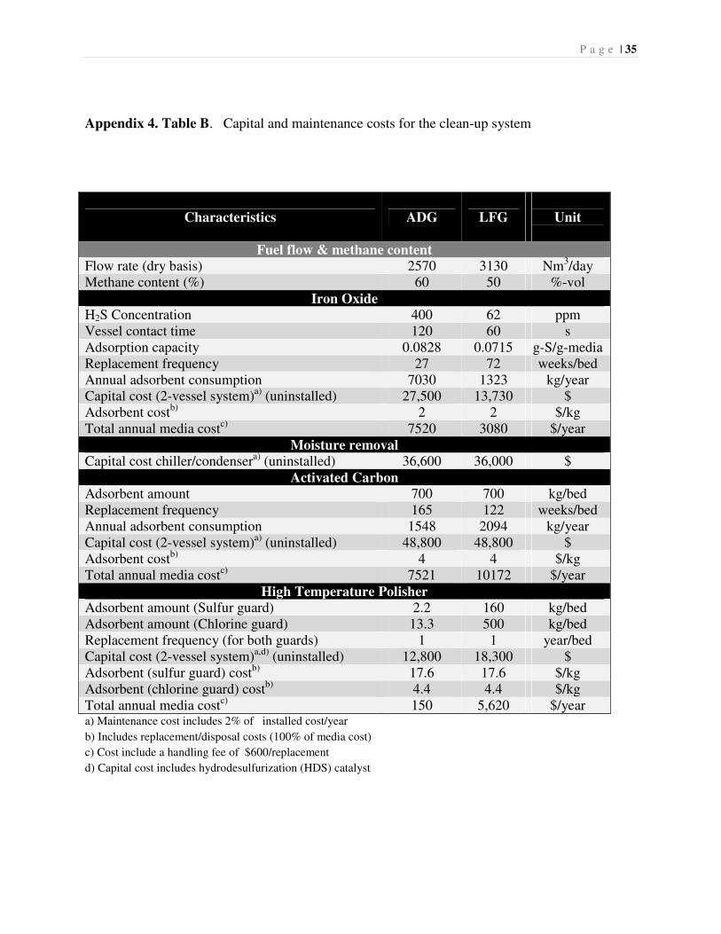
P a g e | 35

Appendix 4. Table B. Capital and maintenance costs for the clean-up system

Characteristics ADG LFG

Unit

Fuel flow & methane content Flow rate (dry basis) 2570 3130 Nm3/day Methane content (%) 60 50 %-vol

Iron Oxide H2S Concentration 400 62 ppm Vessel contact time 120 60 s Adsorption capacity 0.0828 0.0715 g-S/g-media Replacement frequency 27 72 weeks/bed Annual adsorbent consumption 7030 1323 kg/year Capital cost (2-vessel system)a) (uninstalled) 27,500 13,730 $ Adsorbent costb) 2 2 $/kg Total annual media costc) 7520 3080 $/year

Moisture removal Capital cost chiller/condensera) (uninstalled) 36,600 36,000 $

Activated Carbon Adsorbent amount 700 700 kg/bed Replacement frequency 165 122 weeks/bed Annual adsorbent consumption 1548 2094 kg/year Capital cost (2-vessel system)a) (uninstalled) 48,800 48,800 $ Adsorbent costb) 4 4 $/kg Total annual media costc) 7521 10172 $/year

High Temperature Polisher Adsorbent amount (Sulfur guard) 2.2 160 kg/bed Adsorbent amount (Chlorine guard) 13.3 500 kg/bed Replacement frequency (for both guards) 1 1 year/bed Capital cost (2-vessel system)a,d) (uninstalled) 12,800 18,300 $ Adsorbent (sulfur guard) costb) 17.6 17.6 $/kg Adsorbent (chlorine guard) costb) 4.4 4.4 $/kg Total annual media costc) 150 5,620 $/year a) Maintenance cost includes 2% of installed cost/year

b) Includes replacement/disposal costs (100% of media cost)

c) Cost include a handling fee of $600/replacement

d) Capital cost includes hydrodesulfurization (HDS) catalyst

ENERGYU.S. DEPARTMENT OF

Argonne National Laboratory is a U.S. Department of Energy laboratory managed by UChicago Argonne, LLC

Chemical Sciences and Engineering DivisionArgonne National Laboratory9700 South Cass Avenue, Bldg.205Argonne, IL 60439-4837

www.anl.gov

Fuel Quality Issues in Stationary Fuel Cell Systems Quality Issues in Stationary Fuel Cell Systems...

Documents

Transcript of Fuel Quality Issues in Stationary Fuel Cell Systems Quality Issues in Stationary Fuel Cell Systems...