Frequency Domain Analysis of the Random Loading … · Frequency Domain Analysis of the Random...
89
NASA-CR-196021 Frequency Domain Analysis of the Random Loading of Cracked Panels By James F. Doyle, Principal Investigator SCHOOL OF AERONAUTICS AND ASTRONAUTICS PURDUE UNIVERSITY WEST LAFAYETTE, INDIANA 47907 Final Report: For the period October 1, 1990 to September 30, 1993 Prepared for: NASA LANGLEY RESEARCH CENTER HAMPTON, VA 23681-0001 Under: NASA RESEARCH GRANT NAG 1-1173 DR. STEPHEN A. RIZZI, TECHNICAL MONITOR STRUCTURAL ACOUSTICS BRANCH, ACOUSTICS DIV. 4" O" _O ¢¢_ VI ,-4 I **" c_ Z _ 0 z_.u; t- _Z >'Q4a ZO O L ttJO U-Z _t_ _'_ bL P-4 tNI _ CO 0 X0 LU I _- 0 I _')w | I/_ -.IID 0 _D June 16, 1994 https://ntrs.nasa.gov/search.jsp?R=19940031467 2018-07-28T14:13:53+00:00Z
Transcript of Frequency Domain Analysis of the Random Loading … · Frequency Domain Analysis of the Random...

NASA-CR-196021
Frequency Domain Analysis
of the
Random Loading of Cracked Panels
By
James F. Doyle, Principal Investigator
SCHOOL OF AERONAUTICS AND ASTRONAUTICS
PURDUE UNIVERSITY
WEST LAFAYETTE, INDIANA 47907
Final Report:
For the period October 1, 1990 to September 30, 1993
Prepared for:
NASA LANGLEY RESEARCH CENTER
HAMPTON, VA 23681-0001
Under:
NASA RESEARCH GRANT NAG 1-1173
DR. STEPHEN A. RIZZI, TECHNICAL MONITOR
STRUCTURAL ACOUSTICS BRANCH, ACOUSTICS DIV.
4"
O"_O
¢¢_ VI ,-4
I**" c_
Z _ 0
z_.u;t-
_Z
>'Q4a
ZO O L
ttJO
U-Z _t_
_'_ bL P-4
tNI _ CO 0
X0 LU
I _- 0
I _')w |
I/_ -.IID 0
_D
June 16, 1994
https://ntrs.nasa.gov/search.jsp?R=19940031467 2018-07-28T14:13:53+00:00Z

Foreword
This report summarizes the research accomplishments performed under the NASA
langley Research Center Grant No. NAG 1-1173, entitled: "Frequency Domain Anal-
ysis of the Random Loading of Cracked P_nels," for the period October 1, 1990 to
September 30, 1993. The primary effort of this research project was focused on the
development of analytical methods for the accurate prediction of the effect of random
loading on a panel with a crack. Of particular concern was the influence of frequency
on the stress intensity factor behavior.
Contents
2
3
4
Table of Contentsii
Transient Response of Cracked Panels 49
4.1 Finite Element Transient Analysis .................... 49
4.2 Transient Modal Analysis ........................ 50
4.3 Spectral Analysis ............................. 514.4 Discussion
• ° • • * • .... * ...... • • ° ° • • ° • .... • • • * 54
Introduction 1
Outline of Report ............................. 2
Finite Element Modeling 5
1.1 Discrete Kirchhoff Triangular Element• • • • • • • • • • • • • • ° • • 5
1.2 Static Analysis .............................. 8Point Load
• • • • • • • • ° • • • • ° * • • • • • • • ° • • • .... • • • 9
Distributed Load............................. 10
1.3 Vibration Analysis 11• • o • o o • • o • o • • o • • • • • • o ° o o • o • o
1.4 Forced Frequency Spectrum 13• , • .... • . • • o • , • • • , • . • , •
1.5 Modal Analysis .............................. 141.6 Discussion
.... " " • " • .... • • • • ...... • • • • • • .... 16
Static Analysis of Cracked Panels 292.1 Crack in an Infinite Sheet
........................ 292.2 Modified Crack Closure Method ..................... 302.3 Effect of Module Size
........................... 312.4 Effect of Crack Size
............................ 322.5 Discussion
................................. 33
Frequency Domain Analysis of Cracked Panels 39
3.1 Forced Frequency Response Analysis .................. 39
3.2 Virtual Crack Closure Technique 41• o ° . • • • .............
3.3 Global Response Spectrum Method (GRSM) .............. 423.4 Discussion
................................. 43
ii Contents
5
5.1
5.2
5.3
5.4
5.5
5.6
Random Loadings 65
Rand°RanmdomLoL°adadsModad::::::: : : : : : : : : : : : : : : : : : : : : : : 6¢_
Random Load Spectral Analysis ..................... 66
Long Duration Random Loading ..................... 67
Dynamic and Quasistatic Kt Comparison ................ 68Discussion
................................. 69
Conclusions81
References 83
INTRODUCTION
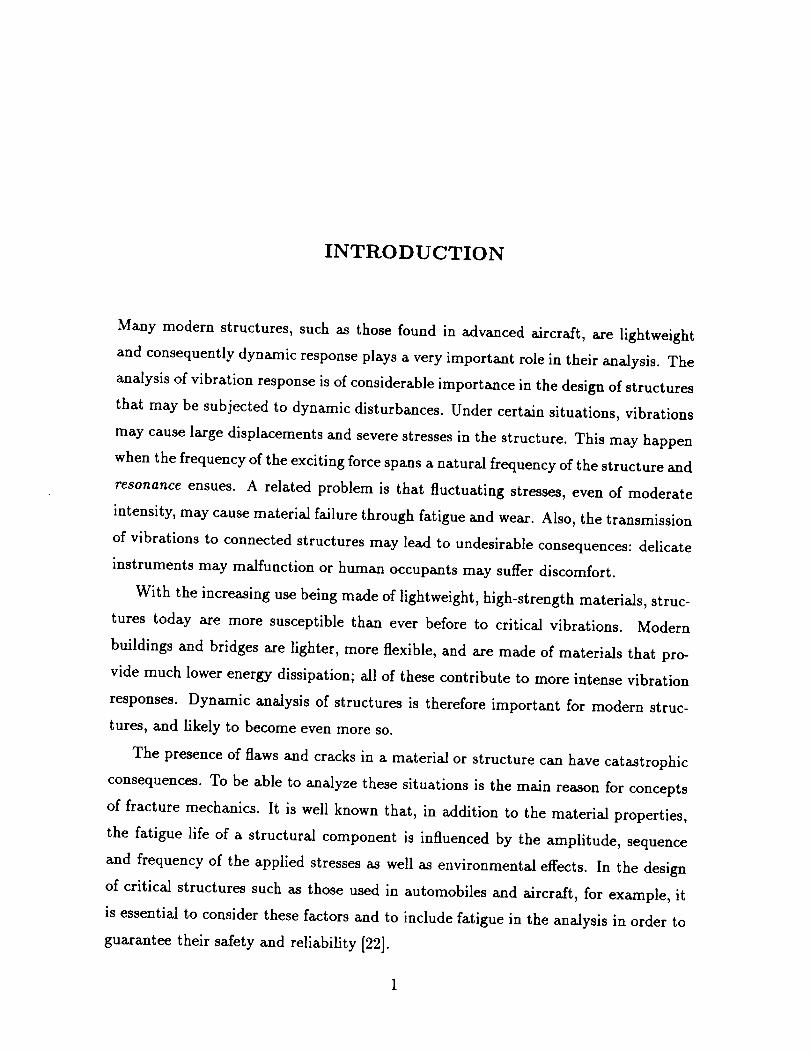
Many modern structures, such as those found in advancedaircraft, are lightweight
and consequentlydynamicresponseplays a very important role in their analysis. The
analysisof vibration responseis of considerableimportance in the designof structures
that may besubjected to dynamic disturbances.Under certain situations, vibrations
may causelargedisplacementsand severestressesin the structure. This may happen
whenthe frequencyof the exciting forcespansa natural frequencyof the structure and
resonanceensues. A related problem is that fluctuating stresses,even of moderate
intensity, may causematerial failure through fatigue and wear. Also, the transmission
of vibrations to connectedstructures may lead to undesirableconsequences:delicate
instruments may malfunction or human occupantsmay suffer discomfort.
With the increasingusebeingmadeof lightweight, high-strength materials, struc-
tures today axe more susceptiblethan ever before to critical vibrations. Modern
buildings and bridgesare lighter, more flexible, and are made of materials that pro-
vide much lower energydissipation; all of thesecontribute to more intensevibration
responses.Dynamic analysisof structures is therefore important for modern struc-tures, and likely to becomeevenmoreso.
The presenceof flawsand cracksin a material or structure canhave catastrophic
consequences.To be able to analyzethesesituations is the main reasonfor concepts
of fracture mechanics. It is well known that, in addition to the material properties,
the fatigue life of a structural component is influenced by the amplitude, sequence
and frequencyof the applied stressesas well asenvironmental effects. In the design
of critical structures suchas those usedin automobilesand aircraft, for example, it
is essentialto considerthesefactors and to include fatigue in the analysis in order to
guaranteetheir safetyand reliability [22].
2 Introduction
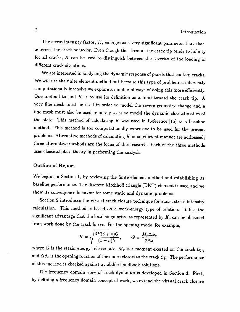
The stress intensity factor, K, emerges as a very significant parameter that char-
acterizes the crack behavior. Even though the stress at the crack tip tends to infinity
for all cracks, K can be used to distinguish between the severity of the loading in
different crack situations.
We are interested in analyzing the dynamic response of panels that contain cracks.
We will use the finite element method but because this type of problem is inherently
computationally intensive we explore a number of ways of doing this more efficiently.
One method to find K is to use its definition as a limit toward the crack tip. A
very fine mesh must be used in order to model the severe geometry change and a
fine mesh must also be used remotely so as to model the dynamic characteristics of
the plate. This method of calculating K was used in Reference [15] as a baseline
method. This method is too computationally expensive to be used for the present
problems. Alternative methods of calculating K in an efficient manner are addressed;
three alternative methods are the focus of this research. Each of the three methods
uses classical plate theory in performing the analysis.
Outline of Report
We begin, in Section 1, by reviewing the finite element method and establishing its
baseline performance. The discrete Kirchhoff triangle (DKT) element is used and we
show its convergence behavior for some static and dynamic problems.
Section 2 introduces the virtual crack closure technique for static stress intensity
calculation. This method is based on a work-energy type of relation. It has the
significant advantage that the local singularity, as represented by K, can be obtained
from work done by the crack forces. For the opening mode, for example,
4/3E(3 + u)G MzA¢_
U:V ' c:where G is the strain energy release rate, M_ is a moment exerted on the crack tip,
and A¢_ is the opening rotation of the nodes closest to the crack tip. The performance
of this method is checked against available handbook solutions.
The frequency domain view of crack dynamics is developed in Section 3. First,
by defining a frequency domain concept of work, we extend the virtual crack closure
3
method to situations involving damping. It is shown that the crack response and
structural response are very similar in character--actually the crack response is dom-
inated by the structural response. This leads to a global response spectrum method
summarized by
k. q_(w): "'" o(0)
where _(_) is the rotation obtained by a modal analysis, ato is its static value, and
K, is the static stress intensity obtained either by analysis or from a handbook. The
essence of this equation is that a 'crack analysis' need only be done for the static case.
Section 4 considers the time responses due to transient loading. There are two
methods investigated: time integrations, and frequency domain convolution repre-
sented by
where/5/(w) is the frequency response function. Each method further divides into
direct use of finite elements or indirectly using modal analysis. The inverse FFT is
taken of the frequency domain quantities in order to find them in the time domain.
The final section considers a very computationally intensive problem--random
dynamic loading of a panel with a crack. Based on the conclusions of Section 4 only
the modal based methods are applied here.
A common thread running through this research is the notion that the dynamics
of cracked panels divides into separate effects of global dynamic behavior of the panel
and local crack tip singularity. In other words, we see an almost static crack embedded
in a structure (sans singularity) which is behaving dynamically. This frees us to bring
to bear the most effective tools for each separate area.

4 Introduction
1. FINITE ELEMENT MODELING
This section reviews the formulation of the finite element modeling and performs some
baseline tests for judging its accuracy. The information gained here will be used to
decide on the model to be used in the later studies. Testing involved different mesh
sizes, boundary conditions, and loadings; whenever possible, the results from the
finite element analysis are compared to the available analytical results. The purpose
of this section is to also exercise the program PlaDyn [13] over the range of problems
to be considered later.
1.1 Discrete Kirchhoff Triangular Element
We consider only thin plate theory (Kirchhoff plates) and the element used to model
this behavior is the discrete Kirchhoff triangle element (DKT). Kirchhoff plate theory
is applied here in that the transverse shear deformation is assumed to be zero; versus
Mindlin plate theory, which assumes transverse shear deformation is allowed. There-
fore, Mindlin plate theory is especially suited to thick plates and sandwich plates [3].
This element has a node at each corner of the triangle with degrees of freedom
{w, Cx, ¢_} at each node. In local coordinates it has a total of 9 degrees of freedom.
In the derivation of the element, the deflection and rotations are assumed to have the
representations (similar to Mindlin plate theory)
6 6 6
i i i
(1.1)
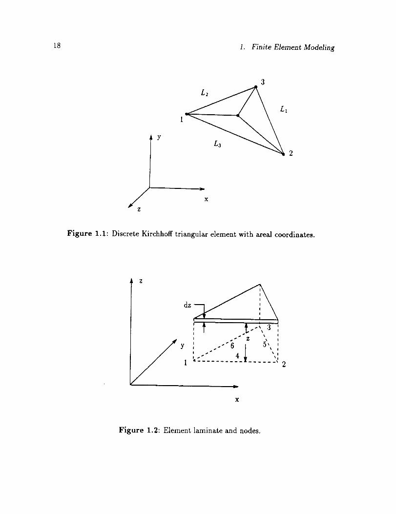
where Ni = (2Li - 1)Li for i=l, 2, 3, N4 = 4LiL2, N5 = 4L_L3 and Ns = 4L3L1. The
parameters Li are areal coordinates and are shown in Figure 1.1. These parameters
can be expressed as
1
Li = -_(A ° + aiz + biy) i = 1,2,3 (1.2)
5
6 1. Finite Element Modeling
where A_', ai, and bi are given as
A'_ = xjyl - xly.i (1.3)
a; = y_ - yt (1.4)
bi = xt - xj (1.5)
where (x,, y_) are the coordinates of the node i (i=1, 2, 3) [12]. In this, there are a total
of 18 unknowns. Hence, initially there are more degrees of freedom than will appear in
the final form of the element. The extra degrees of freedom are eliminated as follows.
The in-plane strains (e_, %, and 7_) are evaluated from the strain-displacement
relations of Mindlin plate theory; consequently, element strains and strain energy
depend on ¢_: and ¢_, but are independent of w. Next, with the shear strains 7zy =
7z_ = 0 in the Mindlin plate equations, we impose Kirchhoff constraints of Ow/Oy -
¢_=0 and Ow/Oz - ¢_=0 at certain points. These particular points are taken at
points midway along the sides, and are sufficient in number to eliminate the extra
degrees of freedom. This leads to the coupling of the rotations with the deflection.
This element was first introduced by Stricklin, Haisler, Tisdale, and Gunderson in
1968 [20]. The derivation of the element is based on requiring the transverse shear
deformation to be zero at the nodes and along the sides of the element and proceeds
as follows.
Consider a laminate of thickness dz located a distance z from the midsurface of
the plate as shown in Figure 1.2. The displacements of this laminate are represented
by
u= z[LI(2L1-1)_-_1 + L_(2L_- 1) _---__
+L3(2L_- l)_-_Uz34LiL Ou, 4L1L3__.U2 ]_-g2+ 4z_L3_u5+Oz oz .!
(1.6)
Ovl Or2= _ ca(2z, - 1)-g2 + L_(2L_- 1)-_-2
- 1)-bTz4_'_-g2 + oz + Oz
(1.7)
1.1 Discrete Kirchhoff Triangular Element 7
_Wl
W = 521(51 -[- 352 -_- 353)Wl -_- i21(c352 _ c253 ) (%/7 (1.8)
_"L _c3wl+i_(b2L3 - _ 2/'_y + ... + ailL_La
where u, v, w are displacements in x, y, and z directions, respectively; L1, L2, La are
area coordinates; bi = yj - Yk; c/ = x_ - xj; and a is a generalized coefficient. The
additional six terms for w are obtained by cyclic permutation.
A nine degree of freedom element is obtained both by requiring the transverse
shear strains to be zero at the corners and along the sides of the element and by
assuming the slope normal to the element at the middle of the side is one half the
sum of the values at the corner nodes. These conditions yield
cgwi Ou_ cOwi Ov_
Ox - --_-z; by -- o')z' i = 1,2, 3 (1.9)
Ou4 113 (ba 2Oz - b_ + c_ -_c3w1+ 2
3
--_C3W2 + (_ _)OU2
_) 0Ul 3b3c3 01) 1--_-z + 4 0z
+ 4 vqzJ
(1.10)
(:9v4 1 [ _ 3. (9ul (_ b_) OVl (1.11)Oz - b_ + c?a - b3wx + _b3c3--_z + Oz
3 3. Ou2
,gzJ
The equations for Ous/Oz, Ovs/Oz, Ou6/Oz, Ou6/Oz are obtained by cyclic permu-
tation. Interelement compatibility is still satisfied after Eqns. 1.9 through 1.11 are
applied.
Neglecting the strain energy due to transverse shear, the strain energy expression
for the element is the same as that used in plane-stress problems;
E l/(e:+ 2 l_v 2 )U - 1 - v 2 2 e_ + 2ve=e_ + ----_--e=_ dAdz (1.12)
where E is Young's modulus, v is Poissons ratio, and the strains are e_ = Ou/Ox,
e_ = Ov/Oz, e_s, = Ou/Oy + 01)�Oz.
It is noted that w does not enter the strain energy expression but enters through
Eqns. 1.9 through 1.11. The element stiffness matrix is obtained by substituting the
8 1. Finite Element Modeling
assumed displacement functions into the strain energy expression and integrating over
the volume of the element using the relation
f i i kL1L L3d`4- + 2)!]2,4 (1.13)
where n = i + j + k and `4 is the area of the element. The element stiffness matrix is
symmetric and positive definite [20].
This DKT element has been widely researched and it has been documented that
it is one of the more efficient elements for thin plate bending. Batoz, Bathe, and
Ho [2] performed extensive testing on three different elements including the hybrid
stress model (HSM), DKT element, and a selective reduced integration (SRI) element.
Comparisons between the different element types were made based on the results
from different mesh orientations and different boundary and loading conditions. The
authors concluded that the DKT and HSM elements are the most effective elements
available for bending analysis of thin plates. Of these two elements the DKT element
was deemed superior to the HSM element based on the comparison between the
experimental and theoretical results [2].
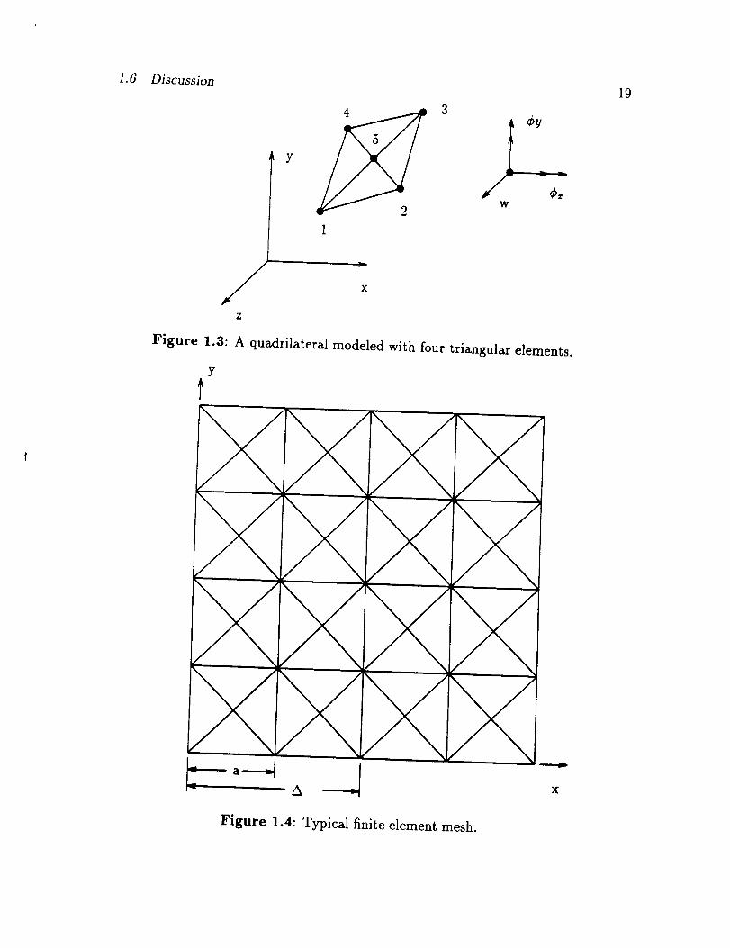
A significant advantage of triangular elements is that they can be conveniently
mapped to form irregular shapes. Our mesh generator uses them to form a basic
building block called a module. A module is a quadrilateral divided into four triangles
(elements) by its diagonals as shown in Figure 1.3. In this way, we effectively have an
arbitrary quadrilateral element with an additional node in the center. This element
is implemented in the finite element package PlaDyn which was used for the analyses.
This progra_rn is capable of performing static and dynamic analysis of folded flat
plates; and it can analyze situations involving applied transient load history, forced
frequency loading, stability analysis, and modal analysis [13].
1.2 Static Analysis
In performing the static analysis, two different boundary conditions for four differ-
ent mesh sizes were considered. The two types of boundary conditions are all edges
simply supported (S-S-S-S), and all edges clamped (C-C-C-C). Two loading condi-
tions were also considered: one was such that a point load was applied at the center
1.2 Static Analysis 9
of the plate, and the other was that of a uniformly distributed load. The meshes
were constructed by using the mesh generating program GenMesh that is part of the
PlaDyn package and a typical mesh is shown in Figure 1.4 . Four different module
sizes were constructed using 2, 1, 0.5 and 0.33 inch (50.8, 25.4, 12.7, and 8.382 mm)
square modules. The plate was 20 inches by 20 inches (508 ram), and the half-plate
used was composed of 200, 800, 3200, and 7200 elements for the respective module
sizes given. In constructing these meshes, symmetry about the y-axis of the panel
was imposed in order to reduce the size of the matrices. From a vibrational point of
view this means that half of the modes will be missing, however, it is deemed that the
number of remaining modes are sufficient to allow adequate testing of the program
and methods. In order to impose the symmetry condition, degrees of freedom were
specified to be u=¢u=O along the mid-plane line of symmetry.
Point Load
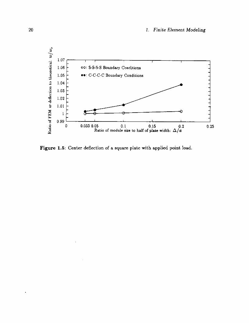
For the S-S-S-S case under point loading the solution for the deflection was derived
in Reference [21]. This particular solution for an applied point load was obtained
using Navier's solution method in double-series form. This double-series converges
very rapidly and the first few terms give the deflection with great accuracy.
For a square plate with a point load applied at the center, the final expression for
the deflection is given by0.0116Pa 2
Wo = D (1.14)
where a is the plate width, P is the applied point load, and D is the flexural rigidity
of the plate given by
Eh 3
D - 12(1 - v 2) (1.15)
In the examples to be discussed, Young's modulus, E, is 10 msi (69 GPa), Poissons
ratio, v, is 0.3 (since this is the value of v that is used in Reference [21]), and plate
thickness, h, is 0.1 inch (2.54 mm). The results are shown in Figure 1.5. What is
encouraging is that even the relatively large module gives very good results.
In deriving the solution for the clamped case, the simply supported solution was
used and superposed on this were the deflections due to moments distributed along
101. Finite Element Modeling
the edges. These moments were adjusted in such a manner as to satisfy the condition
of zero slope along the edges. For a square plate where the point load is applied at
the center, the series converges to
0.00560Pa 2
wo - O (1.16)
Figure 1.5 shows a comparison of the results. For a given mesh size, the deviation
in this case is greater than for the simply supported case. However, as the module
size gets smaller, there is a very nice convergence. Thus, even a module size of 0.5
(A/a=0.05) gives results better than 0.5%.
Distributed Load
In implementing the distributed load for the DKT element, by necessity, different
shape functions must be used for calculating the equivalent load vector than is used
for calculating the stiffness matrix. Through using areal coordinates for the triangle,
we have
{P} (1.17)
PlaDyn forms this equivalent load vector on an element by element basis [13].
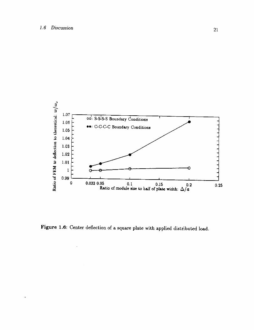
For the S-S-S-S case under uniform loading, the solution was derived in Refer-
ence [21]. In particular for a square plate, the solution is derived in terms of a series
and converges rapidly to give the deflection at the center as
O.O0406qoa 4Wo = D (1.18)
where qo is the magnitude of the uniformly distributed load. The results are shown
in Figure 1.6 and show excellent agreement especially for the smaller module size.
The second set of boundary conditions applied was all edges clamped. Again, the
deflection is derived in terms of a series. For a square plate the series converges to
O.O0126qoa 4
Wo = D (1.19)
The results are shown in Figure 1.6. Again, the finite element results show a very nice
convergence. An explanation for the slight difference may be sought in the nature of
1.3 Vibration Analysis 11
the clamped boundary condition. Most triangles along the boundary have six of the
nine degrees of freedom set to zero, further, twelve of the eighteen degrees of freedom
at a corner (formed by two elements) are set to zero. These conditions are probably
over constraining the finite element solution.
1.3 Vibration Analysis
In performing dynamic problems a choice must be made concerning the method of
assembling the mass matrix. Just as for the distributed load, we cannot give a mass
formulation that is consistent with the DKT element. However, we do have two
alternative formulations; the lumped and consistent mass formulations.
In the lumped mass formulation the total mass, given by pAh, of the element is
equally distributed, or lumped, at each node. No rotational inertias are assumed at
the nodes. The consistent mass matrix formulation is assembled by using displace-
ment functions that are based on areal coordinates and given by
[m] = / p[N]T[N]dV (1.20)
Once the stiffness and mass matrices are assembled, PlaDyn uses the subspace itera-
tion scheme to solve the eigenvalue problem. In this analysis a reduced eigensystem
is established by iteration on a set of Ritz vectors. The advantage in using subspace
iteration (over vector iteration, say) is that the convergence of the subspace and not
of individual iteration vectors is achieved. Consequently, it is less likely to miss any
eigenvectors during the search [11].
The resonant frequencies obtained using the consistent mass formulation were
compared with resonant frequencies obtained using the lumped mass formulation.
This comparison was made so as to determine if using a lumped mass matrix would
yields adequate results. This was of interest since using a lumped mass formulation
versus a consistent mass formulation gives a mass matrix that assembles much quicker,
uses less disk space and also makes the analysis proceed more rapidly
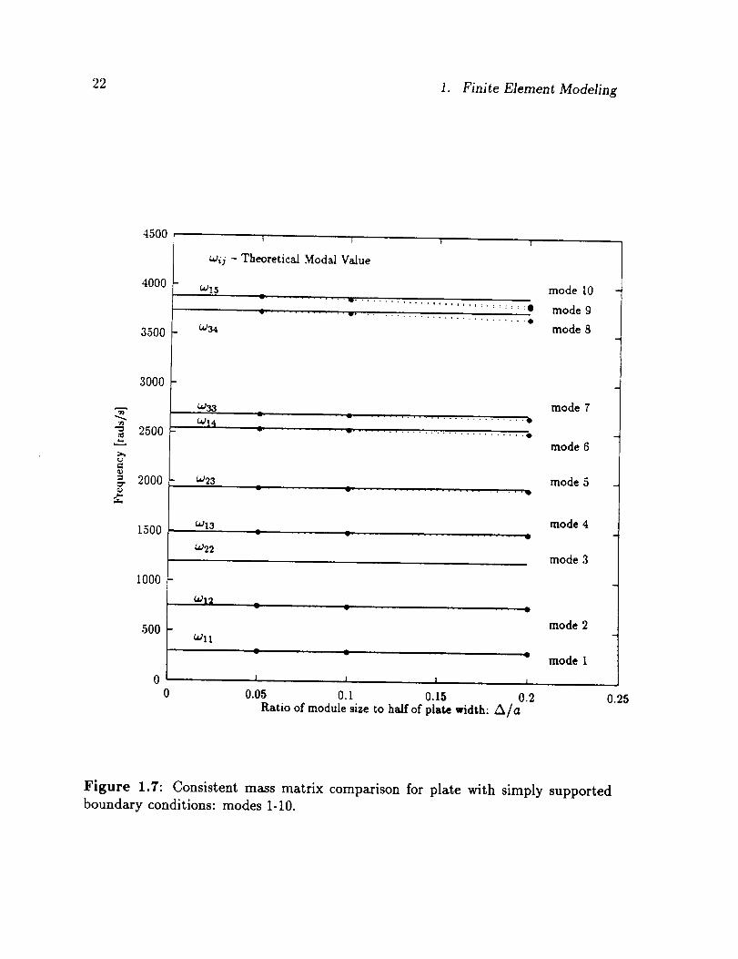
The first boundary condition examined is the S-S-S-S case. Reference [10] gives
12 i.
the following equation for the analytical frequency value:
_'"= T +
Finite Element Modeling
(1.21)
where a and b are the half-widths of the rectangular plate, m and n are the mode
numbers. The results are shown in Figures 1.7 through 1.10. In each case, there is
a very nice convergence to the exact solution as the module size decreases. For each
case, convergence is from below indicating that the stiffness is underestimated or the
mass is overestimated.
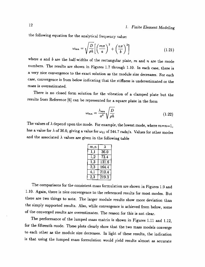
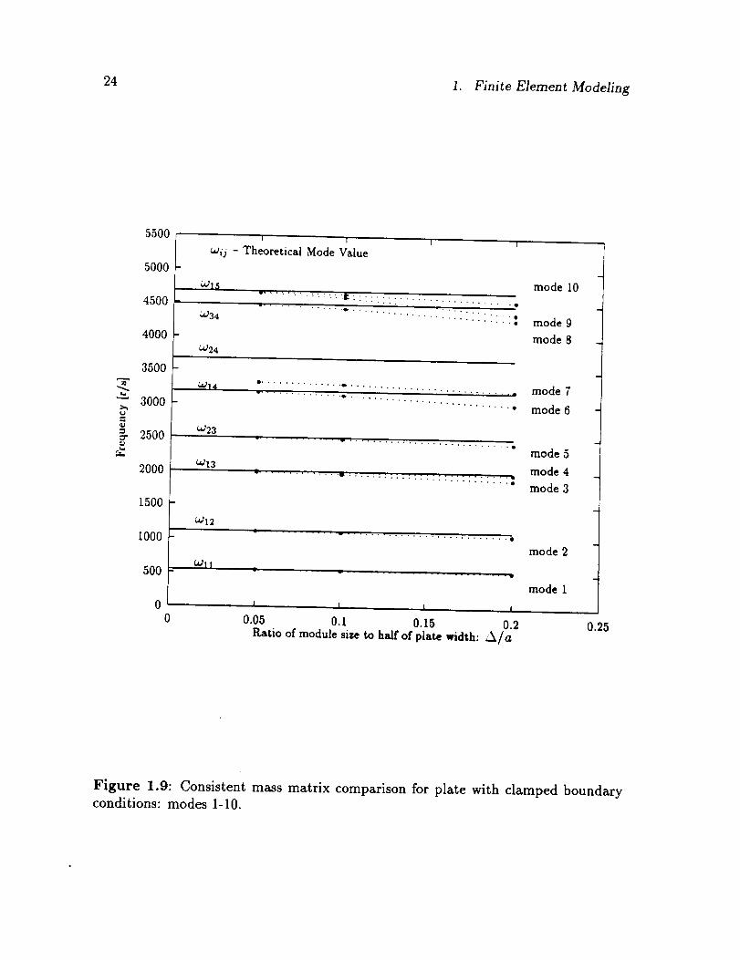
There is no closed form solution for the vibration of a clamped plate but the
results from Reference [6] can be represented for a square plate in the form
win, = _ (1.22)
The values of A depend upon the mode. For example, the lowest mode, where re=n= 1,
has a value for A of 36.0, giving a value for wn of 544.7 rads/s. Values for other modes
and the associated A values are given in the following table
m,n A !
1,1 36.0
1,2 73.4
1,3 131.6
2,3 164.4
4,1 210.4
2,3 219.3
The comparisons for the consistent mass formulation are shown in Figures 1.9 and
1.10. Again, there is nice convergence to the referenced results for most modes. But
there are two things to note. The larger module results show more deviation than
the simply supported results. Also, while convergence is achieved from below, some
of the converged results are overestimates. The reason for this is not clear.
The performance of the lumped mass matrix is shown in Figures 1.11 and 1.12,
for the fifteenth mode. These plots clearly show that the two mass models converge
to each other as the module size decreases. In light of these results, the indication
is that using the lumped mass formulation would yield results almost as accurate
1.4 Forced Frequency Spectrum 13
as the consistent mass formulation. What they also show us, however, is that (for
the simply supported case) when the mesh is marginal (i.e., large module size) the
consistent mass performs better. We have more confidence in the correctness of the
comparison values for this case and hence prefer to draw the conclusions based on it
only.
Generally, since the equivalent of about 20 modes will be considered in the later
sections, it can be concluded that the 0.5 inch (12.7 mm) module with the consistent
mass will be adequate for the frequency range of interest.
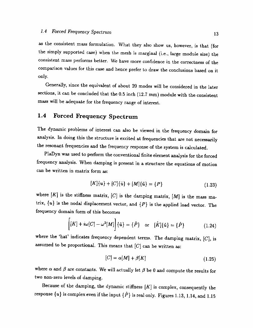
1.4 Forced Frequency Spectrum
The dynamic problems of interest can also be viewed in the frequency domain for
analysis. In doing this the structure is excited at frequencies that are not necessarily
the resonant frequencies and the frequency response of the system is calculated.
PlaDyn was used to perform the conventional finite element analysis for the forced
frequency analysis. When damping is present in a structure the equations of motion
can be written in matrix form as:
[K]{u} + [C]{/_} + [M]{fi} = {P} (1.23)
where [K] is the stiffness matrix, [C] is the damping matrix, [M] is the mass ma-
trix, {u} is the nodal displacement vector, and {P} is the applied load vector. The
frequency domain form of this becomes
[K] + iw[C]-w2[M]] {fi} = {P} or [k']{fi} = {P} (1.24)
where the 'hat' indicates frequency dependent terms. The damping matrix, [C], is
assumed to be proportional. This means that [C] can be written as:
[C] = a[M] +/_[K] (1.25)
where a and _ are constants. We will actually let/_ be 0 and compute the results for
two non-zero levels of damping.
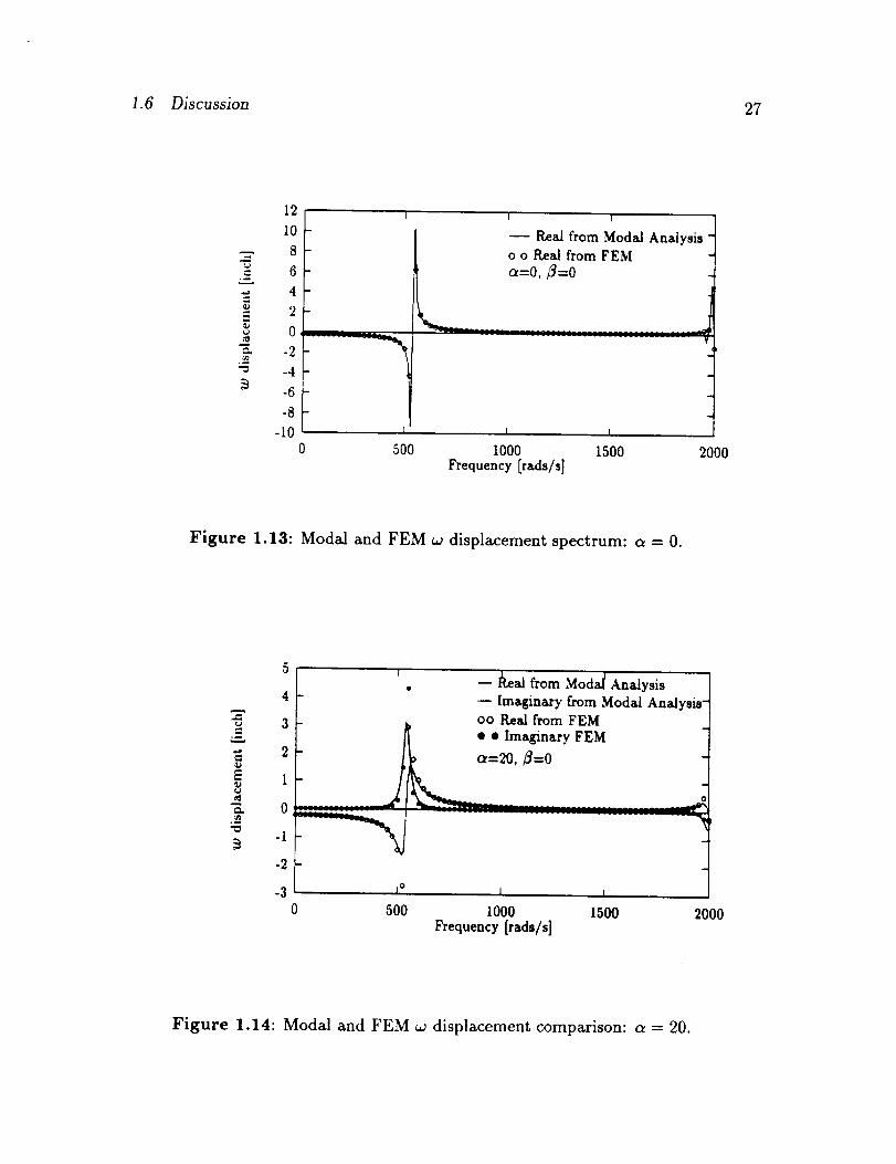
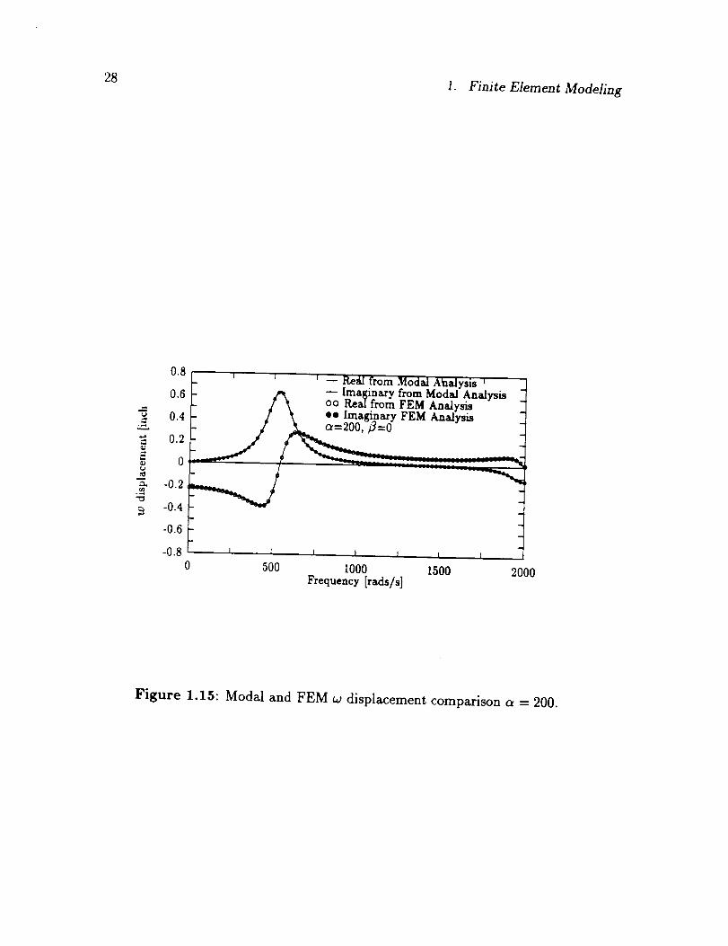
Because of the damping, the dynamic stiffness [K] is complex, consequently the
response {u} is complex even if the input {P} is real only. Figures 1.13, 1.14, and 1.15

14 1. Finite Element Modeling
show the results for values of a = 0, 20, 200, and fl=0 for all cases. A module size
of 0.5 inches (12.7 mm) was used. The range of frequencies span only one resonance.
As expected, increasing the damping decreases the response peak and spreads the
energy among the other frequency components.
1.5 Modal Analysis
When a system consists of many degrees of freedom, it would be beneficial to reduce
the coupled equations of motion to uncoupled algebraic equations. This can be done
by applying modal analysis. Modal analysis uses the concept of the modal matrix
through which the system can be described in terms of uncoupled equations [5].
As part of an eigenanalysis, we obtain the eigenvectors, one for each eigenvalue
or mode. We form the modal matrix by placing these side by side as columns in
an array. This modal matrix has some very useful transformation properties when
applied to the stiffness, mass, and damping matrices. That is,
[_]T[K][_] = rKJ, [¢]T[M][¢] = rMJ, [¢1T[c1[¢1 = rCJ (1.26)
where [KJ, rMJ,and [C'] are diagonal matrices. If we represent the displacements
as
{u} = (1.27)
and substitute this into the equations of motion, then after pre-multiplying by the
modal matrix allows the coupled equations to be written as uncoupled single degree
of freedom systems. The uncoupled system is:
rRj{ } + + rMJ = {_,}/{P} (1.28)
where {r/} is the vector of modal displacements. Since/_i = w_37/i, the above can be
written as
w_yi + 2(iwif]i + _i -
where (, the damping ratio, is defined as
{_}T{p}
#, (1.29)
Ci Ci a +/_w_ (1.30)(i = 2_ 2wiMi - 2wi

1.5 Modal Analysis15
where wi is the modal frequency value. Since less damping is desirable in the higher
modes the values for a used were 0, 20, and 200, and/3 was 0 for all cases.
A standard approach in performing the modal analysis uses the modal displace-
ment method [5]. This method involves solving Eqn. (1.29) for {r/} thereby leading to
a solution to the general equation of motion for the displacement, {u}, and its time
derivatives. A second method could also be used to perform the modal superposition.
This is the modal acceleration method and involves performing a modal transforma-
tion on only the inertia and viscous terms of the equation of motion [12]. This modal
transformation yields the following equation
(u} = [K] -1 (p} -[_]r_j-l((_} + rcj{0}) (1.31)
where r(j is a diagonal matrix with ith diagonal coefficient 2(icoi. In this, the ma-
trix multiplication is carried out over only the lowest m eigenvectors and can be
approximated as
{u} ,_ [K]-'(P} - Z{_}i Oi + 0i (1.32)i----1
where m is less than the number of equations of the system. In order to fully solve
for {u} using the modal acceleration method Eqn. (1.29) is solved for _ and _ for
i ranging from 1 up to m. This is similar to the solution using the modal displace-
ment method. Eqn. (1.32) is used for superposition to obtain {u} as a function of
time [3]. The real advantage in using the modal acceleration method versus the modal
displacement method is that in general fewer modes are required for equivalent accu-
racy. This means that fewer eigenvalues and vectors need be computed thus taking
less computational time. However, it does require solving a static problem for the
complete system. Generally, this is not a significant difficulty but it does mean that
the complete stiffness matrix [K] must be retained. ModDyn [11] is capable of solv-
ing it both ways, but in the following only the mode displacement method is used.
For very large systems, it is generally less expensive to include higher modes than to
retain the stiffness.
The modal displacement method is used by PlaDyn and to account for the effects
of the higher modes, the first 20 modes were taken and the center displacement of
16 I. Finite Element Modeling
the panel was recorded. This number of modes was deemed to be sufficient based on
past comparisons.
Computing the forced frequency spectrums using a modal analysis is very efficient
since for each mode, we have simply
= {¢}m{P}+ _ (1.33)
Figures 1.13, 1.14, and 1.15 show the comparisons with the direct evaluation of
the forced frequency response. The results are generally in good agreement even when
damping is present.
1.6 Discussion
The static and vibrational results establish the DKT element as accurate; they also
give us a set of guidelines to be used when selecting an appropriate mesh size. Gen-
erally, for the panel sizes and frequency range of interest here, a module size of about
0.5 inches (12.7 mm) (Aa/a=O.05) is deemed adequate.
For the modal analysis twenty modes were used to better simulate the panel
behavior. It can be seen from the figures that a good agreement exists between the
finite element and the modal results for the out-of-plane deflection of the center of
the panel. This comparison was performed to establish the relationship between the
modal and the FEM method. Depending upon the desired output, and frequency
range one method may be more adequate to use over the other. For example, if only
a very limited range of frequencies were to be analyzed the FEM method could be
used as the computational time would not be a crucial factor. On the other hand, if a
broad frequency range was of interest, or even more important, if more than one level
of damping was to be analyzed, the modal method would be appropriate. The reason
for this is that for the modal method the computationally intensive portion is the
subspace iteration. For a given model the subspace iteration need only be performed
once. If more than one level of damping was to be analyzed, for example, the actual
analysis portion takes only seconds. If more than one level of damping was to be
analyzed for the FEM method, for each level of damping a separate analysis would

1.6 Discussion 17
need to be performed. This would be computationally expensive and in systems with
a large number of degrees of freedom is not economically feasible.
18 I. Finite Element Modeling
Y
3
L2
LI
1
Figure 1.1: Discrete Kirchhoff triangular element with areal coordinates.
/m ..3 i
I
I oo % !
Y _ ."'6 4 _
1 ................. ' 2
Figure 1.2: Element laminate and nodes.
1.6 Discussion
Y
1
19
X
7.
Figure 1.3: A quadrilateral modeled with four triangular elements.
Y
_-- a--4 IFigure 1.4: Typical finite element mesh.
X
20 I. Finite Element Modeling
.. 1.07
.__1.o61.05
o 1.04
._ 1.03
1.02¢9
_ 1.01
_ 1
e 0.990
I ! ]
oo: S-S-S-S Boundary Conditions
ee: C-C-C-C Boundary Conditions
I !
I I l ! I
0.033 0.05 0.1 0.15 0.2
Ratio of module size to half of plate width: A/a
0.25
Figure 1.5: Center deflection of a square plate with applied point load.
1.6 Discussion 21
.. 1.07
'_ 1.06Q
1.05
o 1.04
.2 1.03
t.02
_ 1.01
_ 1r.r.,
o 0.990
I
oo: S-S_S-S Boundary Conditions '
0 0C ""
I I I I I
0.0330.05 0.i 0.15 0.2
Ratioofmodule sizetohalfofplatewidth:A/a0.25
Figure 1.6: Center deflection of a square plate with applied distributed load.
22 i. Finite Element Modeling
4500
4000
350(
I F
wij - Theoretical Modal Value
i mode 10.......... " ............................. • mode 9
• - " ........ w,
mode 8
"W
3000
2500
2000
1500
i000
5OO
8 • .......................
• II @
0 ' J l j
0 0.05 0.1 0.15 0.2
Ratioofmodule sizetohalfofplatewidth:A/a
mode 7
mode 6
mode 5
mode 4
mode 3
mode 2
mode i
0.2_
Figure 1.7: Consistent mass matrix comparison for plate with simply supportedboundary conditions: modes 1-10.

1.6 Discussion23
¢0
8500
8000
7500
7000
6500
6000
5500
5000
4500
40000
wij - Theoretical Modal Value
mode 20
mode 19mode 18
mode 17
mode 16
mode 15
• . , . . .... . , . . . . . o . . . . . . . , . •
:::::::::::::::::::::::::
mode 14
mode 13
mode 12
...................... Q mode 11L. L .L
0.05 O.1 O.15 0.2 0.25Ratio of module size to half of plate width: A/a
Figure 1.8: Consistent mass matrix comparison for plate with simply supportedboundary conditions: modes 11-20.
24 I. Finite Element Modeling
_J
5500
5000
4500
4000
3500
3000
2500
2000
1500
1000
50O
00
F j
o3ij - Theoretical Mode Value
O315
.:M34
O324
........... ::':iiiiii!!!iiiii!- ............'0
o314
mode i0
mode 9
mode 8
_"................. mode 7• " ........ i|
............ mode 6 -
• . . , , .
od23
OJ13| ..........
0"$12
L ...... v .......
_'_11
I I I I
0.05 0.I 0.15 0.2
Ratioofmodule sizetohalfofplatewidth:A/a
mode 5
mode 4
mode 3
mode 2
mode 1 i
0.25
Figure 1.9: Consistent mass matrix comparison for plate with clamped boundaryconditions: modes 1-10.

1.6 Discussion 25
t_
4_
9500
9000
8500
8000
7500
7000
6500
6000
5500
5000 -
J I I I
_ij - TheoreticM Mode VMue
_J46 • ......I ........ m
¢'_/5S " ' '
_'_36 ' • -
• " " " • • , , "o
¢M45 ..... •
. , , . , , , . . . . , , , ' , , , . . . , . , . • , ,•
• . . , . , . .
_35 "' ''-...
-o . ' ........• . , . . , ....... •
• ' • 'o
_25
• • • • • o.
4500 _ i i ,
0 0.05 0.1 0.15 0.2Ratio of module size to half of plate width: ..k/a
mode 20
mode 19
mode 18
mode 17
mode 18
mode 15
mode 14
mode 13
mode 12
mode 11
0.25
Figure 1.10: Consistent mass matrix comparison for plate with clamped boundaryconditions: modes 11-20.

26 i. Finite Element Modeling
0
--: 4.5
4¢d
'¢ 3.5
-- 33
2.5-
_- 2
_.5
0.5
00
I I F I
oo Lumped Mass Matrix "_
ee Consistent Mass Matrix
Mode 15 Resonant Frequency
S-S-S-S Boundary Conditions
q
0.05 0.1 0.15 0.2 0.25Ratio of module size to half of plate width: -_/a
Figure 1.11: Mass matrix comparison for plate with simply supported boundaryconditions.
5
-j 4.5
4
*¢ 3.5
3o
2.5q_
2
1.5
0,5
0
oo Lumped Mass M_trix [
ee Consistent Mass Matrix /
Mode 15ResonantFrequencyC-C-
T I I
0.05 0.1 0.15 0.2Ratio of module size to half of plate width: _k/a
0.25
Figure 1,12: Mass matrix comparison for plate with clamped boundary conditions.
1.6 Discussion 27
.4
12
i0
8
6
4
2
0
-2
-4
-6
-8
-10
T 7
-- Real from Modal Analysis
o o Real from FEM
a=0, _=0
L J L
0 500 I000 1500
Frequency [rads/s]2000
Figure 1.13: Modal and FEM w displacement spectrum: a = O.
_J
5
4
3
2
1
0
-I
-2
-3
-- l_al from Moda_ Analysis ]Imaginary from Modal Analysis-_
oo Real from FEM !
• • Imaginary FEM
I° I I
0 500 I000 1500
Frequency [r_Is/s]
2000
Figure 1.14: Modal and FEM ._ displacement comparison: a = 20.
28 1. Finite Element Modeling
0.8
0.6
0.4=
"_ 0.2¢D
.=0
-0.2
-0.4
-0.6
I I
-- Re_Ifrom Modal Ahalysis-- ImaginaryfromModal Analysisoo RealfromFEM Analysis
e_Imagin__aryFEM Analysis
-0.8 i _ l j _ 4 l
0 500 I000 1500 2000Frequency[rads/s]
Figure 1.15: Modal and FEM w displacement comparison a = 200.

2. STATIC ANALYSIS OF CRACKED PANELS
Fracture mechanics deals with the conditions under which a body can fail owing to
the propagation of an existing crack of macroscopic size. In the analysis of a structure
containing a crack the key question to be posed is what load will produce failure for
a given crack size, or, for a given loading condition, what will be the allowable crack
size. One of the most important quantities for describing or characterizing a crack
is the stress intensity factor. This is not a stress concentration factor; the difference
being that the former pertains to a singularity in the stress field, whereas the latter
pertains to geometries that do not produce infinite stresses [8].
In this section we investigate the accuracy of the finite element modeling as regards
the analysis of cracks in a panel. Our objective is to help delimit the parameters of
the modeling; that is, establish probable accuracy limits for given meshes and crack
sizes.
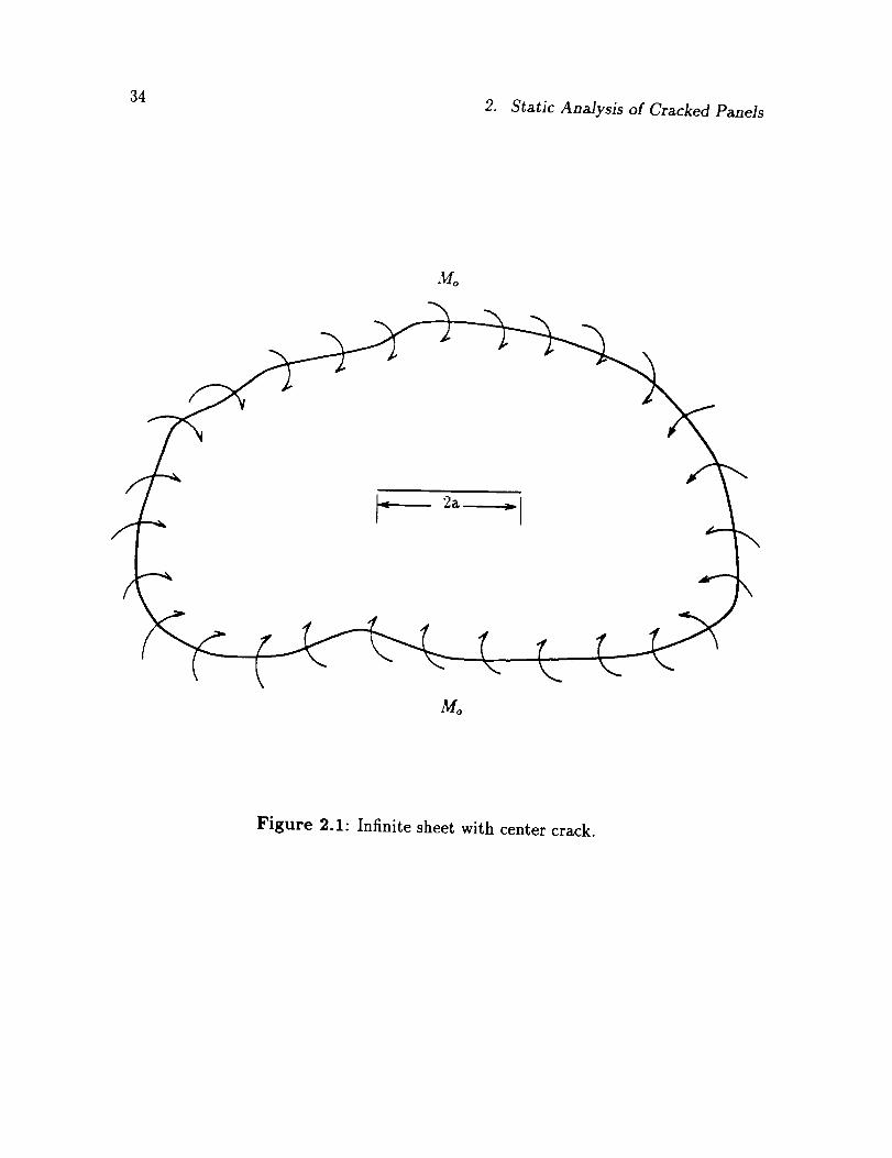
2.1 Crack in an Infinite Sheet
Consider a through-the-thickness central crack in an infinite plate subjected to uni-
form remote bending moment, as shown in Figure 2.1; the stress intensity factor, K/,
can be defined according to the maximum tensile stress as
Kt = lim 2v/2_ra_(r, O, hr-o 3 ) (2.1)
For this plate bending problem, Kz can be expressed as [19]
6MoKI = Ko = aoV#_, ao =
h 2(2.2)
where 114o is the applied uniform moment, a is half the crack length, and h is the plate
thickness. In this way, the stress intensity due to bending can be viewed analogous to
29
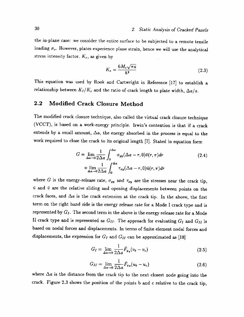
30 2. Static Analysis of Cracked Panels
the in-plane case: we consider the entire surface to be subjected to a remote tensile
loading ao. However, plates experience plane strain, hence we will use the analytical
stress intensity factor, Ko, as given by
Ko_ 6Mov/-_h2 (2.3)
This equation was used by Rook and Cartwright in Reference [17] to establish a
relationship between Kt/Ko and the ratio of crack length to plate width, Aa/a.
2.2 Modified Crack Closure Method
The modified crack closure technique, also called the virtual crack closure technique
(VCCT), is based on a work-energy principle. Irwin's contention is that if a crack
extends by a small amount, Aa, the energy absorbed in the process is equal to the
work required to close the crack to its original length [7]. Stated in equation form
G= lira 1 ["_as 02Aa auu(Aa- r,O)_;(r,_r)dr (2.4)
where G is the energy-release rate, auu and r_ u are the stresses near the crack tip,
and 0 axe the relative sliding and opening displacements between points on the
crack faces, and Aa is the crack extension at the crack tip. In the above, the first
term on the right hand side is the energy release rate for a Mode I crack type and is
represented by Gt. The second term in the above is the energy release rate for a Mode
II crack type and is represented as Gtt. The approach for evaluating GI and Gtt is
based on nodal forces and displacements. In terms of finite element nodal forces and
displacements, the expression for Gt and Gtl can be approximated as [18]
1 -
Gt = a_--,01im-_aFu_(vb- vc) (2.5)
Gtt = lim 1 -a_-_o 2-_aa F_(u_ - uc) (2.6)
where Aa is the distance from the crack tip to the next closest node going into the
crack. Figure 2.3 shows the position of the points b and c relative to the crack tip,

2.3 Effect of Module Size 31
point a. The attractiveness of this method is that the required parameters are few
in number and can be obtained from a single analysis. The latter is important for
dynamic analyses.
The above expressions for the energy release rate are based on in-plane displace-
ments. For the problem of out-of-plane bending of a panel the expression for Gl can
be written as
= -2Aa (2.7)
where M_, is the moment about the crack axis on the crack tip, ¢_b, and ¢_c are the
x-rotations of the nodes closest to the crack tip going into the crack.
For the problem of out-of-plane bending being considered, the stress intensity
factor, K,, for the finite element static case was calculated using the following [23]:
,/3(3 + v)EG
K. : V (2.8)
The program PlaDyn was modified so that it could output these parameters directly.
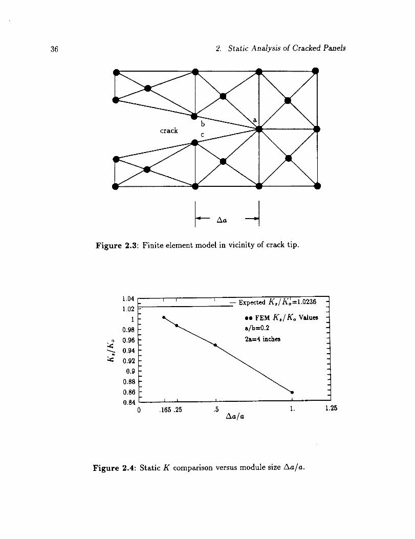
2.3 Effect of Module Size
In order to establish an acceptable model for the cracked panel, calculation of K,
was performed for different module sizes and compared to the handbook values in
Reference [17]. The purpose of this comparison is to establish a module size that can
accurately model the crack tip and the surrounding nodes. Determining the largest
module size was of interest in that a larger module would decrease the amount of disk
space required for storage of the mass and stiffness matrices. But more importantly,
the computational cost in using a larger module size would decrease thus decreasing
actual run time during performing the required analysis.
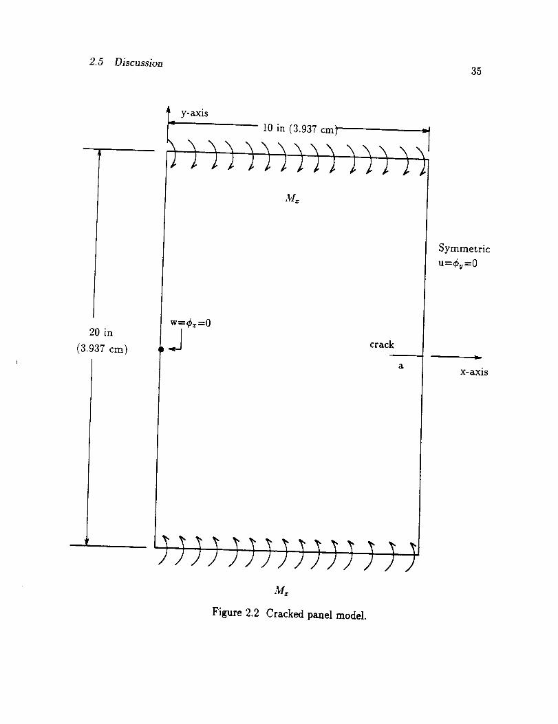
The cracked panel used in this study is shown in Figure 2.2. The model of the panel
was 20 inches (508 mm) wide by 20 inches in length and 0.1 inch (2.54 mm) thick with
a center crack. The material properties of Youngs Modulus, E, shear modulus, G, and
density, p, of the panel were 10.0 msi (69 GPa), 4.0e6 msi (27 GPa), and 2.5E-4 Ib/in 3
(6.93 kg/m3), respectively. Poissons ratio was calculated by v = (E/2G) - 1 = 0.25.
The applied loading consisted of a distributed moment of 10 lb-inches (1.13 N-m).

32 2. Static Analysis of Cracked Panels
This distributed moment was applied along the two edges parallel to the crack length
which was along the z-axis of the panel. Mid-plane symmetry parallel to the y-axis
of the panel was used in order to reduce the amount of disk space required in storing
the stiffness matrix. This crack was 4.0 inches in length. The boundary conditions
imposed were that the node at the center of the plate on each free edge was restricted
in w deflection and ¢_ rotation.
Calculation of the finite element static stress intensity factor, K,, for four differ-
ent module sizes was performed. From Reference [17] the value of K, was given as
Kof(a/b). In this, a is half of the crack length and b is half of the panel width. In our
case we have a/b=0.2 giving f(a/b) of 1.0236 [17]. Using values of Mo=10 lb-inch,
a=2.0 inches (5.08 cm), h=0.1 inches (0.254 cm), and v=0.25, Ko was calculated to
be 15792 lb-inch (1784 N-m); giving a value of 16164 (1826 N-m) for Ko.
The K, value for module sizes of 2, 1, 0.5, and 0.33 inches (Aa/a=l.O, 0.5, 0.25,
and 0.165, respectively) were calculated and Figure 2.4 shows that convergence to the
handbook is being achieved. It should be noted however, that the values from the
handbook are claimed to be accurate to only about 2 percent.
2.4 Effect of Crack Size
We are interested in establishing the adequacy of the mesh for various crack sizes.
To this end, we will keep the module size and panel width constant, and change the
crack length. It is expected that as the crack size approaches the module size that
significant errors will result.
Meshes containing different crack lengths, a, for a constant panel width, b, were
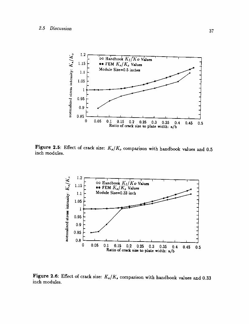
constructed to give different a/b ratios. Figure 2.5 shows the comparison of the
computed Ko/Ko values and the values from the handbook for a module size of 0.5
inches. It can be seen from the figure that for small a/b ratios the results deteriorate
rapidly. This indicates that for small cracks a finer mesh must be used to model the
crack parameters adequately. For a finer mesh model, using modules of 0.33 inches,
Figure 2.6 shows the corresponding comparison. For most of the range, the results
are better, but again there is deterioration at the small crack sizes.
2.5 Discussion
2.5 Discussion
33
The difference between the 0.5 and 0.33 inch module established that using a 0.5
inch module size would yield adequate results. Using the 0.33 inch module size would
give more accuracy, but the advantage of the slightly better results would be at the
expense of the amount of disk space required to store the stiffness and mass matrices.
The most important disadvantage would be in the computational run time. For the
static case the run time for the 0.5 inch module was approximately 10 minutes. For
the case of the 0.33 inch module size it was approximately 18 minutes, or almost 2
times that of the 0.5 inch module size. This computational time difference becomes
even more important when a dynamic analysis is performed and the system must be
solved at each frequency or time step. Therefore, a module size of 0.5 inches was
deemed to give adequate results with regard to the stress intensity factor.
34 2. Static Analysis of Cracked Panels
Mo
Mo
Figure 2.1: Infinite sheet with center crack.
2.5 Discussion35
10 in (3.937 cm)
Symmetric
u=_y =0
20 in
(3.937 cm)crack
M_
Figure 2.2 Cracked panel model.
222
36 2. Static Analysis of Cracked Panels
bcrack
C
Figure 2.3: Finite element model in vicinity of crack tip.
1.04
1.02
i
0.98
0.98
0.94
0.92
0.9
0.88
0.86
0.84
' ' ' -- Expected K,/K_-I.0236 "_
ee FEM K,/Ko Values
a/b=0.2
_.I i I I
.165.25 .5 I._a/a
1.25
Figure 2.4: Static K comparison versus module size Ao/o.
2.5 Discussion 37
1.2..
_" 1.15
1.1
3 1.05
,_-_ 0.95
0.9
" 0.850
'ooH&dboolK_/'A'oV_a._' ' ' 'ss FEM K,/Ko ValuesModule Si = . "
I I I I I I I I I
0.05 0.1 0.15 0.2 0.25 0.3 0.35 0.4 0.45Ratio of crack size to plate width: a/b
0.5
Figure 2.5: Effect of crack size: K,/Ko comparison with handbook values and 0.5inch modules.
1.2
1.15
._1.05
"'_ 1
0.95 -
0.9al-, 0.85s/o= 0.8
0
t I I I I I l I I
oo iI;_ lHandbook Ko Values
ss FEM Ks Values
Module Size_
" _ . "
3/I I I I 1 I I I I
0.05 0.1 0.15 0.2 0.25 0.3 0.35 0.4 0.45Ratio of crack size to plate width: a/b
0.5
Figure 2.6: Effect of crack size: Ko/K_ comparison with handbook values and 0.33inch modules.

38 2. Static Analysis of Cracked Panels
3. FREQUENCY DOMAIN ANALYSIS OF CRACKED
PANELS
Some dynamic analyses are more easily performed in the frequency domain, in par-
ticular, the dynamic output for structures that exhibit resonant type behavior is
more easily interpreted. It will be shown that the stress intensity factor also exhibits
resonant type behavior similar to the structure as a whole.
The stress intensity factor, K, is required in order to perform analysis for fatigue
crack propagation. Since various crack geometries need to be considered, a K calibra-
tion would be required for each different geometry. This process is expensive in the
static case alone but in the frequency domain it is even more so since the calibration
must be done over a wide spectrum of frequencies
Two methods for calculating the frequency domain stress intensity factor, K(w),
will be investigated. The first is a variation of the Virtual Crack Closure Technique
(VCCT) but applied in the frequency domain to damped systems. The second method
combines a modal analysis with a static crack analysis to obtain the variation in
the frequency domain. For all of this analysis, one of the restrictions made on the
modeling is that the crack is 'open' during vibration. This means that the faces of the
crack do not touch during the vibration. This is at least consistent with the general
approach to cracks in flexure.
3.1 Forced Frequency Response Analysis
Forced frequency means that the structure is excited at frequencies that are not
necessarily the resonant frequencies. One of the primary differences between modal
and finite element methods is how the damping is input. The damping for the finite
element analysis is taken to be proportional so that we can relate the results to the
39
40 3. Frequency Domain Analysis o[ Cracked Panels
modal analysis. When damping is present in a structure, the equations of motion can
be written in the frequency domain as
[[K] + iw[C]-w2[M]]{fi} = {P} (3.1)
The damping matrix, [C], is assumed to be proportional in the form
[C] = a[M] + fl[K] (3.2)
where a, and /_ are constants. In the forced frequency problem we can solve for
{fi} over many frequencies. These displacements, which are complex in general, can
then be used to obtain the moments and stresses, say, also as a function of frequency.
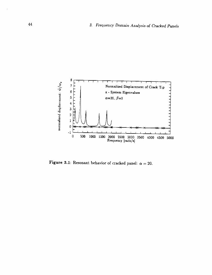
Figure 3.1 shows the displacement of the panel of Figure 2.2 as a function of frequency
for medium damping.
The out-of-plane displacement of the crack tip was normalized with respect to its
static value. The resonant frequencies are indicated by x marks on the figure. It can
be seen that the peaks of the displacement normal occur near the resonant frequency
indicating the resonant behavior of the panel. We are interested in characterizing
the behavior of the range of about 2000 rads/s, as seen this will include about five
resonances.
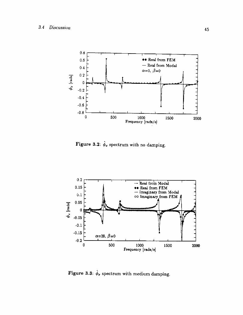
The finite element and modal analysis for Cx at the crack tip, was performed for
damping values of a of 0, 20, and 200 and a/_ value of 0 for all cases. The results are
shown in Figures 3.2, 3.3, and 3.4. From these figures there is good agreement between
the finite element and modal Cx results. Figure 3.3 shows the spectral behavior of ¢=
with medium damping. It exhibits the classical resonance behavior in that the real
component goes through a zero while the imaginary component goes through a peak.
A forced frequency modal analysis was also performed for the model in Figure 2.2.
The modal analysis package ModDyn was used for this purpose. The system can be
written as
2 {¢}T{p}w,_r/m + 2(,_wm_,, + _,_ -
Mm (3.3)
where _', the damping ratio, is obtained as
2win (3.4)
3.2 VirtuM Crack Closure Technique 41
Figures 3.2 to 3.4 show the results. For the case in which there is no damping
present, the results for the two methods discussed show good agreement. When
damping is added to the system the comparisons remain in good agreement especially
for the lower damping value of a=20. For the higher level of damping value, a=200,
the system response exhibited characteristics of being overdamped. Figure 3.4 shows
that the agreement was quite good for this case also.
3.2 Virtual Crack Closure Technique
The purpose of this subsection is to modify the concept of the virtual crack closure
technique for use in the frequency domain when the response functions are complex.
We can consider all response variables transformed into the frequency domain. In
particular, we have for the stress
,,,,,,(x,y, t) y,,,,) (3.5)
We now take as our definition for the frequency domain stress intensity factor
k(w) -!im_5_(r, o,w) (3.6)
This, in fact could be used as a numerical scheme for K-extraction. It is expected
that the value of/_ will be linear (when plotted against v/'}) in the region dominated
by the singularity of the crack tip and therefore linear extrapolation to r = 0 can be
used [9, 15]. In order to use this method a very fine mesh around the crack tip must
be used; using a fine mesh makes the analysis computationally expensive, hence this
method will not be investigated here. We seek alternative methods.
Irwin's contention is that if a crack extended a small amount, Aa, then the energy
absorbed in the process is equal to the work required to close the tip of the extended
crack to its original length. This is essentially an equivalency between work done
and energy stored. In the frequency domal,, all of our quantities are complex and
frequency dependent, hence we introduce a complex work term defined as
dI?V = Pd_ (3.7)
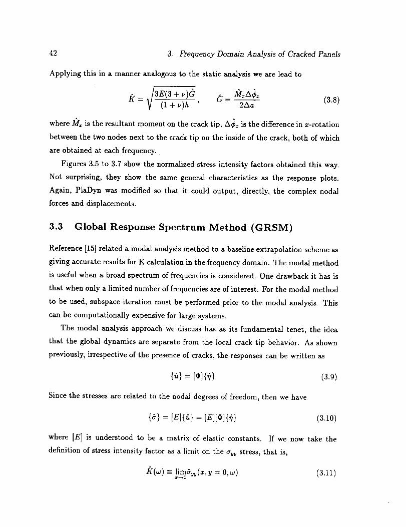
42 3. Frequency Domain Analysis of Cracked Panels
Applying this in a manner analogous to the static analysis we are lead to
,/3E(3 + v)G __ 214r::A¢=K= v _+_)h ' 2Aa (3.S)
where JI;/= is the resultant moment on the crack tip, A¢_ is the difference in z-rotation
between the two nodes next to the crack tip on the inside of the crack, both of which
are obtained at each frequency.
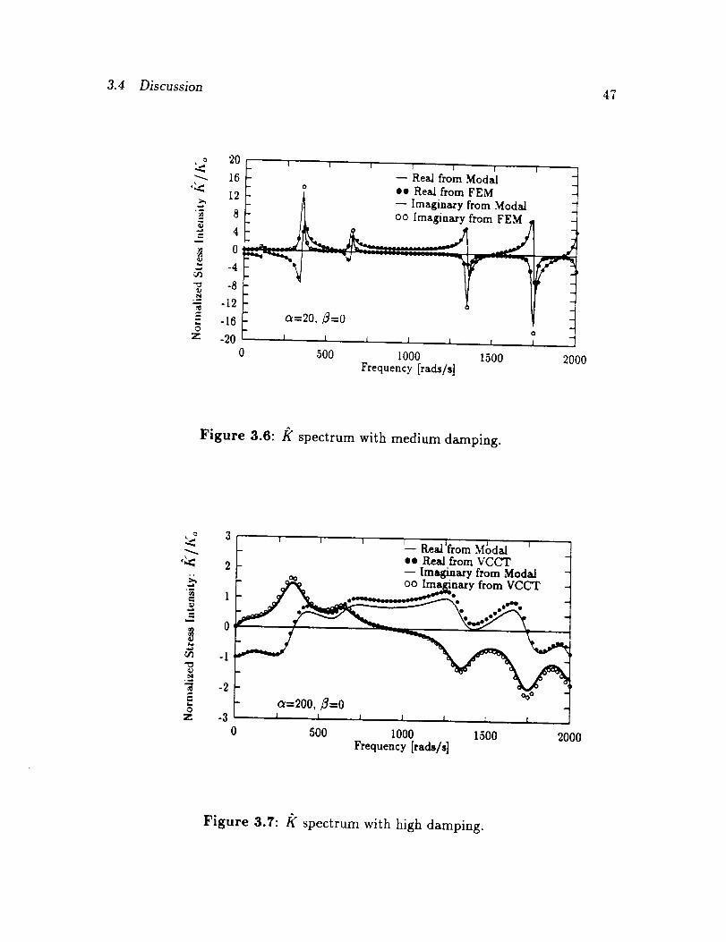
Figures 3.5 to 3.7 show the normalized stress intensity factors obtained this way.
Not surprising, they show the same general characteristics as the response plots.
Again, PlaDyn was modified so that it could output, directly, the complex nodal
forces and displacements.
3.3 Global Response Spectrum Method (GRSM)
Reference [15] related a modal analysis method to a baseline extrapolation scheme as
giving accurate results for K calculation in the frequency domain. The modal method
is useful when a broad spectrum of frequencies is considered. One drawback it has is
that when only a limited number of frequencies are of interest. For the modal method
to be used, subspace iteration must be performed prior to the modal analysis. This
can be computationally expensive for large systems.
The modal analysis approach we discuss has as its fundamental tenet, the idea
that the global dynamics are separate from the local crack tip behavior. As shown
previously, irrespective of the presence of cracks, the responses can be written as
=
Since the stresses axe related to the nodal degrees of freedom, then we have
(3.9)
{5} = [E]{fi} = [E][(I)]{,)} (3.10)
where [E] is understood to be a matrix of elastic constants. If we now take the
definition of stress intensity factor as a limit on the av, j stress, that is,
k(w) = limS_v(z,y = 0,w) (3.11)x--t0

3.4 Discussion 43
we see that we must have
/_(w) = 7[¢]{I)} (3.12)
where 7 is some constant. In other words,/_(w) must exhibit the same type of modal
behavior as all the other quantities.
We can obtain 7 from a static analysis (i.e., the special case When ca=O) and are
thus lead to
/_(w) = Ks ¢(w) g_= (3.13)
where ¢(w) is a significant response function, ¢o is its static value, and K, is the static
stress intensity value. We can obtain K, from a handbook such as Reference [17] if
it is available. In our case, we have
K.=Kof(a/b), go- 6M°h2 (3.14)
where 3/0 is the applied moment. Alternatively, we can obtain K, directly from a
static analysis as was done here.
The stress intensity spectrums are shown in Figures 3.5, 3.6, and 3.7 for damping
values of a = 0, 20, and 200, respectively. In general, they follow closely the results
from the virtual crack closure technique.
3.4 Discussion
In general, the results of the virtual crack closure technique and the global response
spectrum method were in good agreement. This conclusion is important. Since
both methods give equivalent results then we have a greater freedom in choosing a
method for a particular problem. For example, if only a limited range of frequencies
are to be analyzed, the virtual crack closure method could be used. On the other
hand, if a broad frequency spectrum is of interest (which would be the case if time
reconstructions are to be performed) the modal method would be appropriate. For the
modal method the computationally intensive portion is the eigenanalysis and this cost
can be distributed over the large number of frequencies. The cost of the actual modal
summation portion is insignificant. The direct forced frequency solution using finite
elements does not enjoy such a speed up, as each frequency calculation is independent.
44 3. Frequency Domain Analysis of Cracked Panels
-2
.m
t_
8
7
6
5
4
3
2
I
0
-I
Normalized Displacement of Crack Tip
x - System gigenvalues
ct=20,/3=0
m
I
I I I Z i i L i I I I
0 500 I000 1500 2000 2500 3000 3500 4000 4500 5000Frequency [rads/s]
Figure 3.1: Resonant behavior of cracked panel: a = 20.
3.4 Discussion 45
0.8
0.6
0.4
0.2
g o
-0.4
-0.6
-0.8
"_"_['--__T_T T T
- T ee Realfrom FEM
[ ---Real=fromModal
0 500 1000 1500 2000Frequency[fads/s]
Figure 3.2: ¢= spectrum with no damping.
0.2
0.15
0.I
0.05¢1
0
-e- -0.05
-0.1
-0.15
-0.2
' ' ' -- _eal frown Moda_ '
ee Real from FEM: -- Imaginary from Modal
I l l l
500 1000 1500Frequency [rads/s]
J
2000
Figure 3.3: Cx spectrum with medium damping.

46 3. Frequency Domain Analysis of Cracked Panels
4
0.0,3
0.02
0.01
0
-0.01
-0.02
-0.030
Figure 3.4: ¢_ spectrum with high damping.
.4
U
8z
60
40
20
0
-20
-40
-60
I l
L_
I 1 I I
ee RealfromVCCT
-- RealfromModal
a=0, 3=0
Jr--
i
I I I I i J
0 500 I000 1500
Frequency[rads/s]2000
Figure 3.5: /( spectrum with no damping.
3.4 Discussion 47
o 2O
16
12
4
0
_Z -4
._ -12e-
" -16
z -200
- -- Realfrom ModalO
ee RealfromFEMImaginaryfrom Modal
oo Imaginaryfrom FEM
o=20, fl=O
5OO
0
1000 1500FrequencyIra(is/s]
T"--"--
2000
Figure 3.6: /_" spectrum with medium damping.
3
'_ 2
-= 0
-2
z -30
- ' _ ' _ Real Ifrom M_dal ' _]_ ee Real from VCCT 7
oo -- Imaginary from Modal -4- _ oo Ima_nary from VCCT -" J' 'S. ... • ••e •
- o=200, fl=O ooo -I I I I I ; I
500 I000 1500 2000Frequency[rads/s]
Figure 3.7: /_" spectrum with high damping.

48 3. Frequency Domain Analysis of Cracked Panels
4. TRANSIENT RESPONSE OF CRACKED PANELS
If a structure is excited by a suddenly applied, short term, excitation the response is
said to be a transient or impact response. After the force has stopped the structure
will then eventually exhibit free vibrations. If damping is present the vibrations will
then decay over time.
In this section we are interested in determining the time history response of a
panel with a crack. The first method uses direct time integration of the system
of equations. This was performed using PlaDyn. The second method uses modal
summation. The modal analysis was performed using the modal analysis package
ModDyn. The third technique uses a spectral approach where frequency response
functions are first obtained and then transformed to the time domain by the inverse
fast Fourier transform (FFT).
4.1 Finite Element Transient Analysis
For the transient analysis of the panel, the equations of motion are written as
[K]{u} + [C]{/L} + [M]{fi} = (P} (4.1)
The applied force {P} is a function of time and is written as {P}(t) = {p}P(t), where
{p} is a vector representing the time independent distribution of forces. For the panel
as used in the previous section, say, {p} consists (mostly) of unit moments applied at
each top and bottom boundary node. P(t) is the input function of time and is shown
in Figure 4.1 and its amplitude spectrum is shown in Figure 4.2.
In performing the finite element transient analysis, eqn. 4.1 was time integrated
using Newmark implicit time integration. For the integration the time step was chosen
to be 50/_s with 400 time steps giving a time window of 0.02 seconds.
49
50 4. Transient Response of Cracked Panels
The transient finite element results from PlaDyn for the rotation are shown in
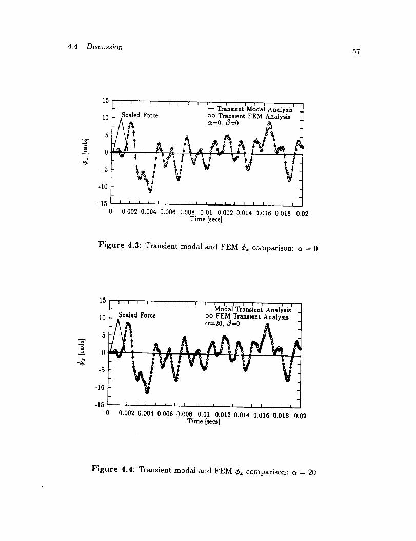
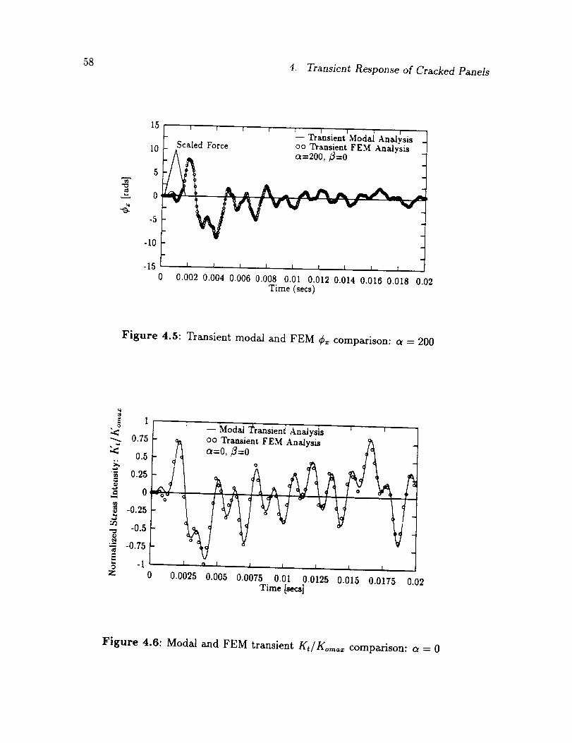
Figures 4.3, 4.4, and 4.5, for damping values of 0, 20, and 200 for at, with _ being 0
for all cases. It is seen that the effect of damping is noticeable only at the long time.
The initial transient response settles into a vibration with what appears to be two
dominant modes.
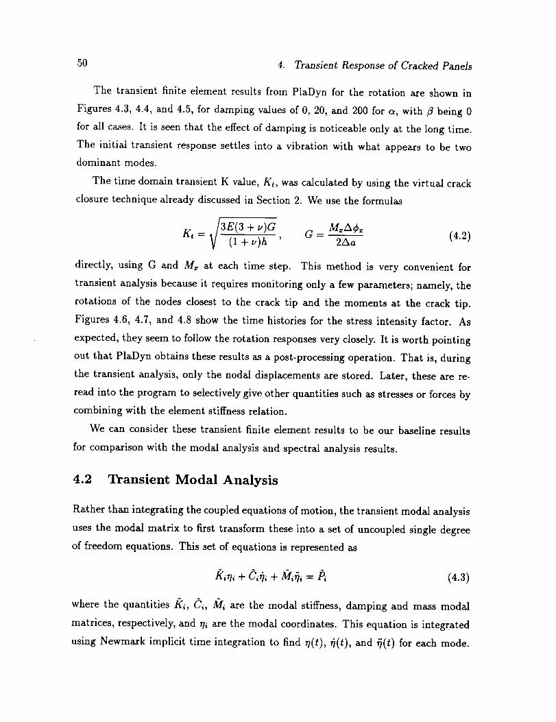
The time domain transient K value, Kt, was calculated by using the virtual crack
closure technique already discussed in Section 2. We use the formulas
,/3E(3 + v)G M_A¢_
Kt = V -_ _ -v)-h ' G- 2,'%a(4.2)
directly, using G and Ms at each time step. This method is very convenient for
transient analysis because it requires monitoring only a few parameters; namely, the
rotations of the nodes closest to the crack tip and the moments at the crack tip.
Figures 4.6, 4.7, and 4.8 show the time histories for the stress intensity factor. As
expected, they seem to follow the rotation responses very closely. It is worth pointing
out that PlaDyn obtains these results as a post-processing operation. That is, during
the transient analysis, only the nodal displacements are stored. Later, these are re-
read into the program to selectively give other quantities such as stresses or forces by
combining with the element stiffness relation.
We can consider these transient finite element results to be our baseline results
for comparison with the modal analysis and spectral analysis results.
4.2 Transient Modal Analysis
Rather than integrating the coupled equations of motion, the transient modal analysis
uses the modal matrix to first transform these into a set of uncoupled single degree
of freedom equations. This set of equations is represented as
(4.3)
where the quantities/_i, _',, __/_ are the modal stiffness, damping and mass modal
matrices, respectively, and rh are the modal coordinates. This equation is integrated
using Newmark implicit time integration to find r/(t), O(t), and _(t) for each mode.
4.3 Spectral Analysis 51
Again, as for the finite element analysis, the time integration step used was 50/Js with
400 time steps. The separate modes are then recombined to give the actual response
as
{u}(t) = [¢]{r/}(t ) (4.4)
where {u}(t) is the displacement vector corresponding to the original finite element
analysis. The advantage of this approach is that it allows the selection of the range
of modes that participate in the response--these are generally much lower than the
system size. Initially, 20 modes were used for the analysis. But, based on later results
the number of modes was increased to 30. Increasing the number of modes takes into
account more of the structure; thus making the results better.
A transient analysis using modes in the summation was performed. Figures 4.3, 4.4
and 4.5 show the comparison between the modal and finite element results for _. The
comparisons are seen to be good. This is to be expected since both methods employ
the same discretization of the system and the same integration scheme of Newmark
implicit time integration. Hence as long as the number of modes is adequate, the
correspondence should almost be exact.
The Kt calculation for the modal analysis was based on the same VCCT equation
as the finite element analysis. The one difficulty with this formulation is that the
moment on the crack tip is needed. Since the modal analysis calculates displacement
responses of the system only, a scheme had to be devised to obtain the force on the
crack tip associated with the displacements. We did this by using ModDyn to create
the post-processing file of displacements for use by PlaDyn. PlaDyn was then used
to perform the force history analysis based on these modal displacements.
Figures 4.6, 4.7, and 4.8 show the comparison with the finite element results.
Again, as expected the agreement is very close.
4.3 Spectral Analysis
When the response of a given panel due to different loading histories is required, a
transient analysis for each loading must be performed. For a system with a large
number of degrees of freedom this is computationally expensive. Spectral analysis
52 4. Transient Response of Cracked Panels
is a scheme that can be used to avoid this by allowing convenient frequency domain
convolutions with the applied force. This is illustrated here.
In spectral analysis, a time history is given the representation [4]
u(xl,y,,t) = E fi"(x'Y'W")(w)e'W"' (4.5)
where u(t) is the time response, fi,, is the spectrum of amplitudes, and w,_ are the
frequencies. In the frequency domain, the response due to a load can be written as
=/:L,P (4.6)
where/;/_ is the transfer function. Once this is known then the simple product above
(called a convolution) with a different/5 is used to get the response to different load
histories.
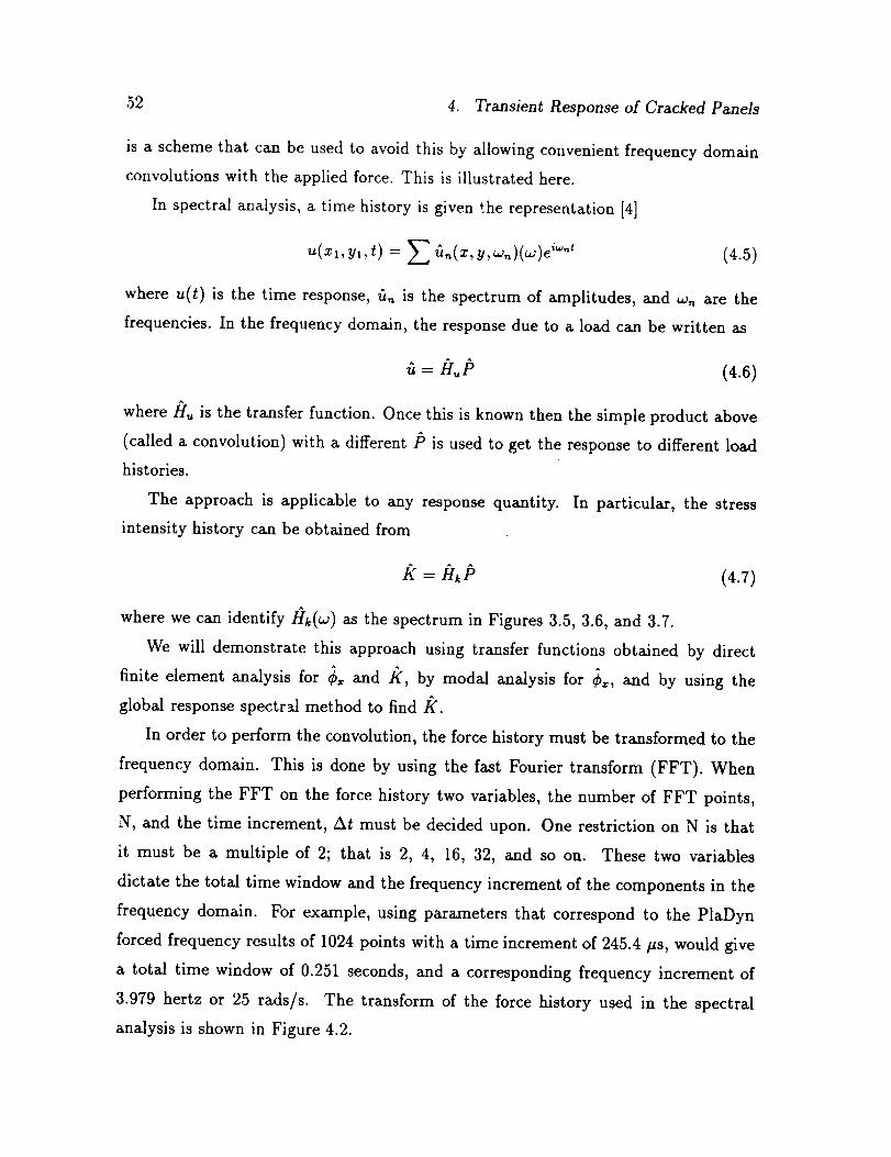
The approach is applicable to any response quantity. In particular, the stress
intensity history can be obtained from
/f =/:/kP (4.7)
where we can identify Hk(w) as the spectrum in Figures 3.5, 3.6, and 3.7.
We will demonstrate this approach using transfer functions obtained by direct
finite element analysis for ¢_ and K, by modal analysis for ¢_, and by using the
global response spectr_ method to find K.
In order to perform the convolution, the force history must be transformed to the
frequency domain. This is done by using the fast Fourier transform (FFT). When
performing the FFT on the force history two variables, the number of FFT points,
N, and the time increment, At must be decided upon. One restriction on N is that
it must be a multiple of 2; that is 2, 4, 16, 32, and so on. These two variables
dictate the total time window and the frequency increment of the components in the
frequency domain. For example, using parameters that correspond to the PlaDyn
forced frequency results of 1024 points with a time increment of 245.4 #s, would give
a total time window of 0.251 seconds, and a corresponding frequency increment of
3.979 hertz or 25 rads/s. The transform of the force history used in the spectral
analysis is shown in Figure 4.2.
4.3 Spectral Analysis 53
It has been established in the earlier parts of this section that there is a correlation
between the trend exhibited by the rotation ¢, and the stress intensity factor. Thus,
an initial indication of how closely the stress intensity factor will match the baseline
finite element results is achieved by comparing the inverse FFT of the convolution
of the force transform and the frequency domain ¢, values. The results for this axe
shown in Figure 4.9, 4.10 for damping values of a=20, and 200, and/3=0, respectively.
Initially, the comparison between the finite element inverse FFT rotation values
and the baseline finite element rotation values showed some disagreement. This dif-
ference was caused by the limited frequency spectrum of the forced frequency finite
element results. Only 81 points were taken in the forced frequency finite element
analysis because of long computational time. Therefore, when/?/was convolved with
the transform of the force a very limited range of the force was used. This was cor-
rected by broadening the spectrum of the finite element forced frequency analysis.
When this frequency spectrum was convolved with the force transform more of the
force was used; therefore, giving more non-zero points when taking the inverse FFT
and giving better results when compared to the baseline FEM results as shown in
Figures 4.9 and 4.10.
The/_" values calculated using the broader frequency spectrum values were used
as the transfer function and the convolution with the transform of the force was
performed. The inverse FFT was taken and the comparison between the results and
the finite element baseline results axe shown in Figures 4.11, and 4.12 for damping
values of a = 20 and 200, respectively, and 0 for/3. The Kt values were normalized
by using
Ko,-,,_ = 6M°P(t)m_v/-_h2 (4.S)
where P(t),,,_ is the peak value of the scaling history shown in Figure 4.1. As
expected, the agreement with the baseline finite element results is very close.
The forced frequency modal analysis can be performed at any number of frequency
intervals for many frequency steps. This was because once the eigenanalysis, which
is the computationally expensive portion of the modal analysis, is done, the modal
summation takes a relatively short time to execute. A frequency increment of 10
54 4. Transient Response of Cracked Panels
rads/s was used for 1000 frequency steps. Using this number of frequency steps
takes the frequency spectrum out to the Nyquist of the force transform. Taking the
modal frequency spectrum out to the Nyquist enables the full force amplitude to be
used when the convolution is taken between the modal transfer functions and the
transform of the force. The comparison between these results and the baseline finite
element transient ¢, values are shown in Figure 4.13, and 4.14 for the two damping
values. The results were again normalized similarly to the finite element results. The
results seem to be very close. In fact they are about the same as obtained in the time
integration scheme.
The/( values found by using the GRSM method were used as the transfer function
and convolved with the transform of the force. Figures 4.15, and 4.16 show that the
comparison between the GRSM reconstruction values and the baseline finite element
results are again in good agreement.
4.4 Discussion
The choice of a particular method for transient analysis depends upon the type of
problem to be examined. If, for example, a limited time window is to be examined
then the finite element method with direct integration may be used since the number
of time steps would be small. On the other hand, if multiple loading histories are
to be used or responses over a very long time are required then the modal methods
are indicated since only one eigenanalysis would be required. This is mentioned since
in the modal analysis this is the part that is computationally intensive. The actual
summation portion takes a short amount of time and can be performed for a variety
of damping values and force histories.
The use of the spectral method gives an alternative to the two methods mentioned
above. In this, a single forced frequency analysis is performed and by convolving with
the transform of the applied load and performing an inverse fast Fourier transform,
the results in the time domain for different load histories can be found. This method
can be very useful if a single model is to be examined over a variety of input load
histories. The comparisons shown above illustrate that if an adequate number of

4.4 Discussion 55
transform points are taken, the spectral method will yield results comparable to
those that would be obtained by either method previously mentioned.
We thus have four alternative methods for calculating K(t), the stress intensity
factor in the time domain. The choice of using the particular method should be based
on problem parameters such as if multiple analysis for the same model, if multiple
levels of damping are to considered and the time window of interest.

56 4. Transient Response of Cracked Panels
.=1
o
1200
1000
800
600
400
200
0
-200'0
1 [ I I I I I I I
ment-- Envelope
I I 1 1 I I I I I
0.000;5 0.001 0.0015 0.002 0.0025Time [secs]
Figure 4.1: Applied load history.
.=s_
"6_D
¢U
z.
0.8
0.7
0.6
0.5
0.4
0.3
0.2
0.I
0
-0.I
I I 1 I
-- Magnitude of the Moment Transform- System Eigenvalues
I I I I
5000 10000 15000 20000 25000FrequencyIra,s/s]
Figure 4.2: Transform of applied load history.
4.4 Discussion 57
t=,
4
-O-
15
10
5
0
-5
-10
-15
- -- Transient Modal Analysis
Scaled Force oo Transient FEM Analysis
0 0.002 0.004 0.006 0.008 0.01 0.012 0.014 0.016 0.018 0.02Time [sees]
Figure 4.3: Transient modal and FEM ¢= comparison: a = 0
15
10
5
-5
-10
-150
-- Modal TransientAnalysisScaled Force oo FEM TransientAnalysis =
0.002 0.004 0.006 0.008 0.01 0.012 0.014 0.016 0.018 0.02Time [sees]
Figure 4.4: Transient modal and FEM ¢. comparison: a = 20
58 4. Transient Response of Cracked Panels
15
10
5
0
-5
-10
-150
I 1 I 1
Scaled Force
I I ! i I
-- Transient Modal Analysisoo Transient FEM Analysisa=200, fl=O
I
I I I I I I I 1 I
0.002 0.004 0.006 0.008 0.01 0.012 0.014 0.016 0.018Time (secs)
0.02
Figure 4.5: Transient modal and FEM ¢2 comparison: a = 200
0.75
k_ 0.5
"_ 0.25
_= 0
i -0.25
-0.5
-0.75
-Iz 0
oo Transient FEM Analysis _
4=0, ° f] /
0.0025 0.005 0.0075 0.01 0.0125 0.015 0.0175 0.02Time [sees]
Figure 4.6: Modal and FEM transient Kt/Kom.= comparison: a = 0

4.4 Discussion 59
2
B4
z
0.75
0.50.25
0
-0.25
-0.5 {-0.75
-1 -...__...1..___0 0.0025
-- Modal TransientAnalysis
oo FEM TransientAnalysis _ -
0.005 0.0075 0.01 0.0125 0.015 0.0175 0.02Time [sees]
Figure 4.7: Modal and FEM transient Kt/K,_,,. comparison: a = 20
,° 1
0.75
0.5
0.25
2 0
i -0.25-0.5
_. -0.75
z -I0
_r-------_ l r--=--=r----__T -----.--Modal TranientAnalysis
oo FEM TransientAnalysis -
a=200,i3=0
0.0025 0.005 0.0075 0.01 0.0125 0.015 0.0175 0.02Time [secs]
Figure 4.8: Modal and FEM transient Kt/Kom,, comparison: a = 200
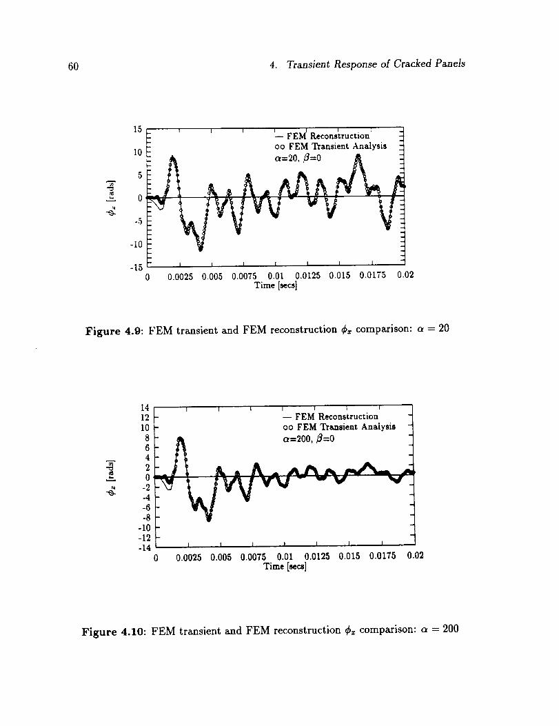
60 4. Transient Response o[ Cracked Panels
15
10
5
0
-5
-i0
-15
I ] I l ] ] [
FEM Reconstructionoo FEM TransientAnalysis =-
a:20, _:0 A :
- I I I i I I I
0 0.0025 0.005 0.0075 0.01 0.0125 0.015 0.0175 0.02Time [secs]
Figure 4.9: FEM transient and FEM reconstruction ¢= comparison: a = 20
4
141210
4
-2-4
-10-12-14
I l I I I I I
- -- FEM Reconstruction
- oo FEM TransientAnalysis
Ct:200, _=0
A,, _-
vv- -" --:_
I I I I I J l
0 0.0025 0.005 0.0075 0.01 0.0125 0.015 0.0175Time [secs]
0.02
Figure 4.10: FEM transient and FEM reconstruction ¢= comparison: a = 200
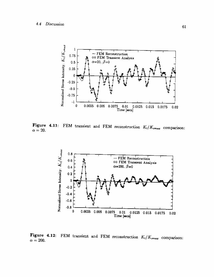
4.4 Discussion 61
N¢1
I _---_-_ M r'------rReconstruction0.75
0.5
'_ 0.25
_= 0
-0.25
-0.5
-0.75
-Iz
t 1 r
=2o, 3=o ,,
oo FEM TransientAnalysis
i
<b
0 0.0025 0.005 0.0075 0.01 0.0125 0.015 0.0175 0.02Time [secs]
Figure 4.11: FEM transient and FEM reconstruction Kt/Ko_,,= comparison:a=20.
0.8
_-_ 0.60.4
"_ 0.2
0
-0.2-0.4
-o.s
_r"---'__v---"'-r-------_ T T-- FEM Reconstructionoo FEM TransientAnalysis
a=200, fl=0
-0.8 _.__..__
Z 0 0.0025 0.005 0.0075 0.01 0.0125 0.015 0.0175 0.02Time [secs]
Figure 4.12: FEM transient and FEM reconstruction Kt/Kom_= comparison:a = 200.
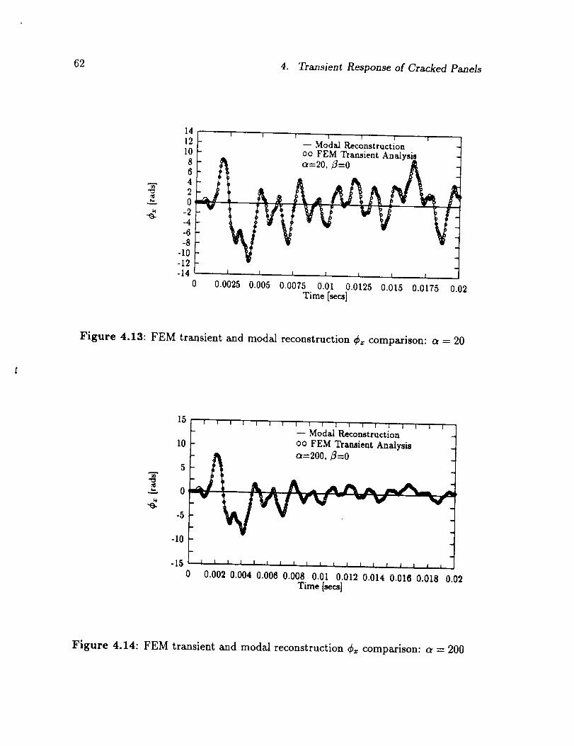
62 4. Transient Response of Cracked Panels
7
141210
4
-2-4-6-8-I0-12 --14 __
0
_T-'-'-'-_r--------_ r T "r_Modal Reconstruction
oo FEM TransientAnalys_
0.0025 0.005 0.0075 0.01 0.0125 0,015 0.0175 0.02Time [secs]
Figure 4.13: FEM transient and modal reconstruction _ comparison: a = 20
15
10
5
-5
-10
J _ _ J _ J _ _ _ _ z _ _ _ _ j _ _- -- Modal Reconstruction _
oo FEM TransientAnalysis
-15 J i i I I I i I I I I l i I f I l l i
0 0.0020.0040.008 0.008 0.01 0.0120.014 0.016 0.018 0.02Time [secs]
Figure 4.14: FEM transient and modal reconstruction _ comparison: a = 200
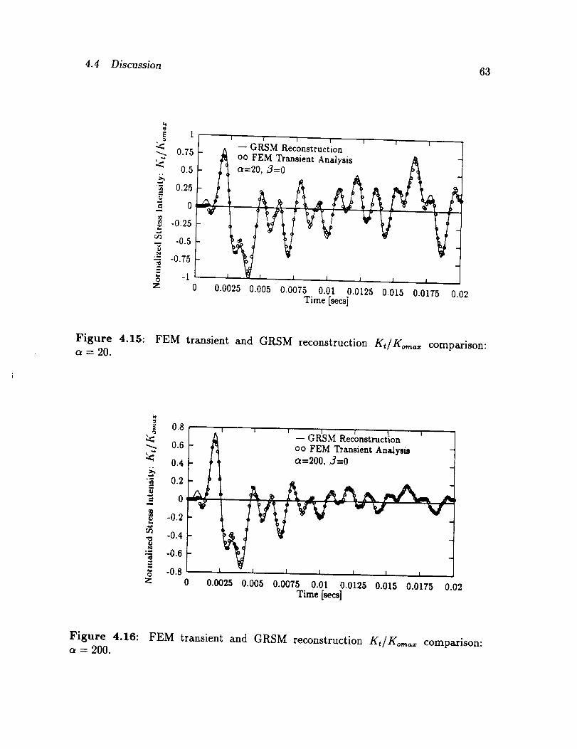
4.4 Discussion 63
4
_. 0.75
0.5
"_ 0.25
= 0
-0.25
-0.5N
-0.75
-1z 0
I I I I I I I
-- GRSM Reconstruction
OO :_FEMTransient Analysis
, • Ct--29 d
c I I 1 1 I I
0.0025 0.005 0.0075 0.01 0.0125 0.015 0.0175 0.02Time [secs]
Figure 4.15: FEM transient and GRSM reconstruction Kt/Ko,,,_= comparison:a=20.
0.8 I "------F-'----_--
_. 0.6
0.4 * *
"_ 0.2 ° *
o- @-
-0.2 .
._ -0.4
"_ -0.6r-
-0.8z
V---'---'T--r----'---I--T-- t
-- GRSM Reconstruction
oo FEM TransientAnalysis
e=200, A=0
0 0.0025 0.005 0.0075 0.01 0.0125 0.015 0.0175 0.02Time [sees]
Figure 4.16: FEM transient and GRSM reconstruction Kt/Ko,,,,= comparison:a = 200.

64 4. Transient Response of Cracked Panels
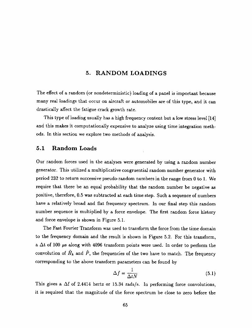
5. RANDOM LOADINGS
The effect of a random (or nondeterministic) loading of a panel is important because
many real loadings that occur on aircraft or automobiles are of this type, and it can
drastically affect the fatigue crack growth rate.
This type of loading usually has a high frequency content but a low stress level [14]
and this makes it computationally expensive to analyze using time integration meth-
ods. In this section we explore two methods of analysis.
5.1 Random Loads
Our random forces used in the analyses were generated by using a random number
generator. This utilized a multiplicative congruential random number generator with
period 232 to return successive pseudo-random numbers in the range from 0 to 1. We
require that there be an equal probability that the random number be negative as
positive, therefore, 0.5 was subtracted at each time step. Such a sequence of numbers
have a relatively broad and flat frequency spectrum. In our final step this random
number sequence is multiplied by a force envelope. The first random force history
and force envelope is shown in Figure 5.1.
The Fast Fourier Transform was used to transform the force from the time domain
to the frequency domain and the result is shown in Figure 5.2. For this transform,
a At of 100 /_s along with 4096 transform points were used. In order to perform the
convolution of/:/k and P, the frequencies of the two have to match. The frequency
corresponding to the above transform parameters can be found by
1
Af _ Atg (5.1)
This gives a Af of 2.4414 hertz or 15.34 rads/s. In performing force convolutions,
it is required that the magnitude of the force spectrum be close to zero before the
65
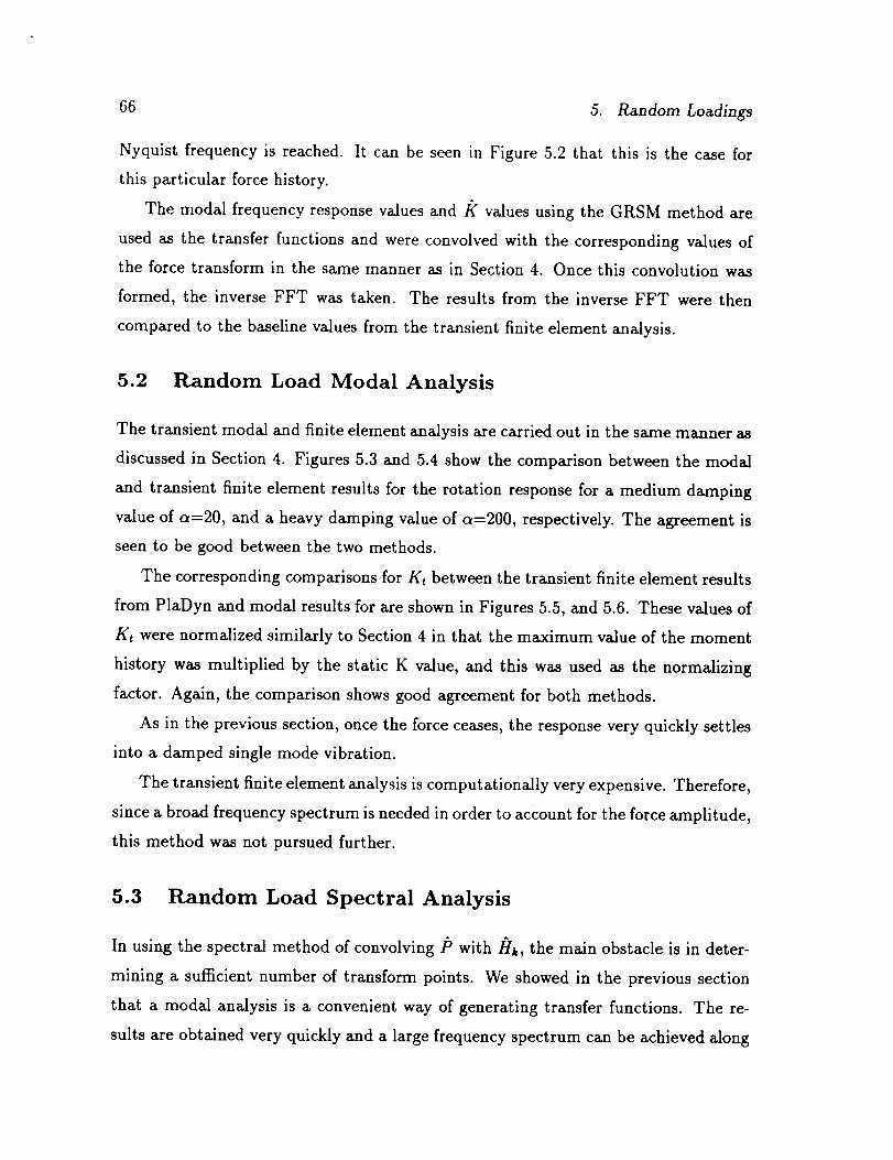
66 5. Random Loadings
Nyquist frequency is reached. It can be seen in Figure 5.2 that this is the case for
this particular force history.
The modal frequency response values and/t" values using the GRSM method are
used as the transfer functions and were convolved with the corresponding values of
the force transform in the same manner as in Section 4. Once this convolution was
formed, the inverse FFT was taken. The results from the inverse FFT were then
compared to the baseline values from the transient finite element analysis.
5.2 Random Load Modal Analysis
The transient modal and finite element analysis axe carried out in the same manner as
discussed in Section 4. Figures 5.3 and 5.4 show the comparison between the modal
and transient finite element results for the rotation response for a medium damping
value of a=20, and a heavy damping value of a=200, respectively. The agreement is
seen to be good between the two methods.
The corresponding comparisons for Kt between the transient finite element results
from PlaDyn and modal results for axe shown in Figures 5.5, and 5.6. These values of
Kt were normalized similarly to Section 4 in that the maximum value of the moment
history was multiplied by the static K value, and this was used as the normalizing
factor. Again, the comparison shows good agreement for both methods.
As in the previous section, once the force ceases, the response very quickly settles
into a damped single mode vibration.
The transient finite element analysis is computationally very expensive. Therefore,
since a broad frequency spectrum is needed in order to account for the force amplitude,
this method was not pursued further.
5.3 Random Load Spectral Analysis
In using the spectral method of convolving/5 with/;/k, the main obstacle is in deter-
mining a sufficient number of transform points. We showed in the previous section
that a modal analysis is a convenient way of generating transfer functions. The re-
sults are obtained very quickly and a large frequency spectrum can be achieved along
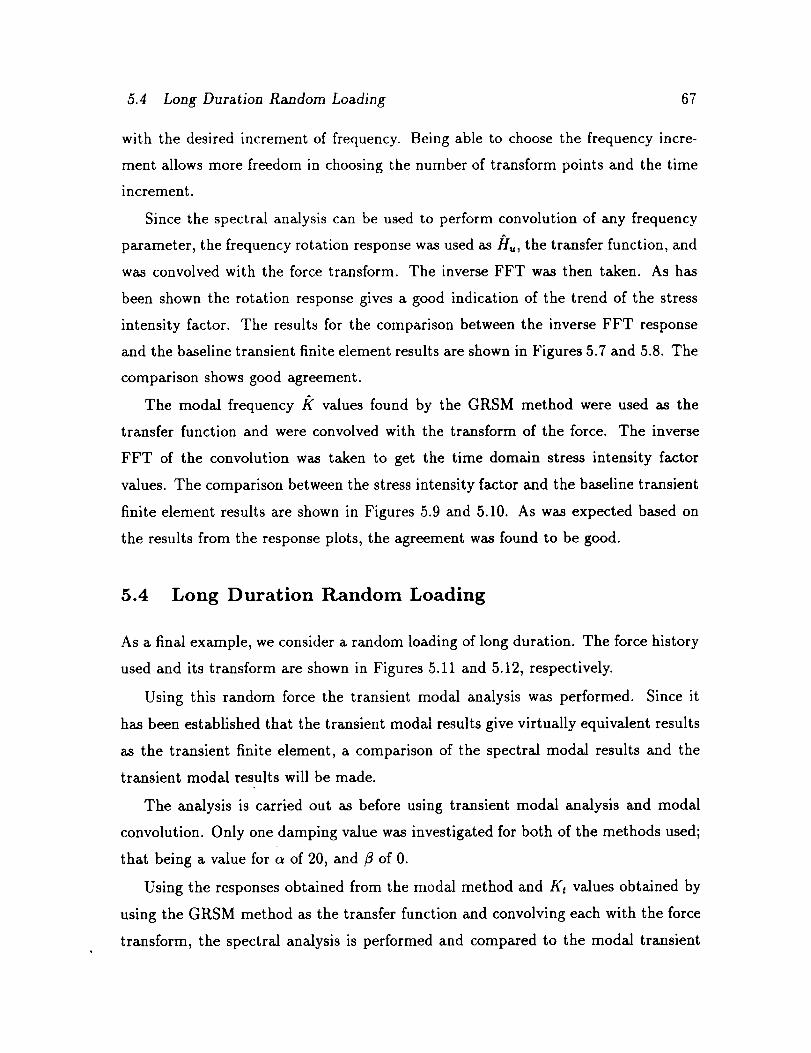
5.4 Long Duration Random Loading 67
with the desired increment of frequency. Being able to choose the frequency incre-
ment allows more freedom in choosing the number of transform points and the time
increment.
Since the spectral analysis can be used to perform convolution of any frequency
parameter, the frequency rotation response was used as//_, the transfer function, and
was convolved with the force transform. The inverse FFT was then taken. As has
been shown the rotation response gives a good indication of the trend of the stress
intensity factor. The results for the comparison between the inverse FFT response
and the baseline transient finite element results are shown in Figures 5.7 and 5.8. The
comparison shows good agreement.
The modal frequency /_ values found by the GRSM method were used as the
transfer function and were convolved with the transform of the force. The inverse
FFT of the convolution was taken to get the time domain stress intensity factor
values. The comparison between the stress intensity factor and the baseline transient
finite element results are shown in Figures 5.9 and 5.10. As was expected based on
the results from the response plots, the agreement was found to be good.
5.4 Long Duration Random Loading
As a final example, we consider a random loading of long duration. The force history
used and its transform are shown in Figures 5.11 and 5.12, respectively.
Using this random force the transient modal analysis was performed. Since it
has been established that the transient modal results give virtually equivalent results
as the transient finite element, a comparison of the spectral modal results and the
transient modal results will be made.
The analysis is carried out as before using transient modal analysis and modal
convolution. Only one damping value was investigated for both of the methods used;
that being a value for a of 20, and fl of 0.
Using the responses obtained from the modal method and Kt values obtained by
using the GRSM method as the transfer function and convolving each with the force
transform, the spectral analysis is performed and compared to the modal transient

68 5. Random Loadings
results. Figure 5.13 shows the comparison for the rotation response. Figure 5.15
shows the _omparison of the transient Kt values. As was expected, the they axe in
good agreement.
A note should be made regarding the time increment chosen for the integration
and the transform. It was found that the time increment used for taking the force
transform had little effect on the results after the inverse FFT was taken and compared
to previous results. On the other hand, the time increment chosen to generate the
modal responses in order to do the post processing to gain the moment on the crack tip
had a significant effect on the results. The time increment of 100/_s in taking the force
transform was used. An initial value of 50_s was used in the modal transient analysis.
Upon comparing the ¢_ and Kt values, it was seen that the agreement was not very
good. Therefore, a finer time step was used for the modal transient integration and
the comparison for these results are shown in Figures 5.14 and 5.16 on a reduced
time scale for ease of comparison for the rotation and Kt results, respectively. These
results show good agreement between the two methods.
5.5 Dynamic and Quasistatic Kt Comparison
The dynamic problem studied above will be put into perspective by considering the
quasistatic problem. By quasistatic, we mean that for each discretized random load
point the corresponding Kt value would be calculated by
gt = go = 6M°P(t)v/-_h2 (5.2)
where Mo is the constant applied moment, and P(t) is its scaling history time. For
the random force the K, values were calculated and normalized with respect to the
K value found by using the maximum moment of 500 in the above equation for P(t).
These results were then compared to the Kt values calculated for the modal transient
analysis in the previous section. The comparison is shown in Figure 5.17. As can
be expected the quasistatic Kt values follow the same pattern as exhibited by the
random input. It can be seen that the values from the dynamic response and the
quasistatic analysis are drastically different--as much as 400% on average. One of
the reasons for the large difference is that for the dynamic analysis multiple resonances
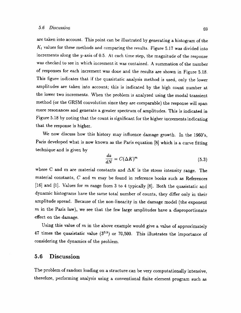
5.6 Discussion 69
are taken into account. This point can be illustrated by generating a histogram of the
Kt values for these methods and comparing the results. Figure 5.17 was divided into
increments along the y-axis of 0.5. At each time step, the magnitude of the response
was checked to see in which increment it was contained. A summation of the number
of responses for each increment was done and the results are shown in Figure 5.18.
This figure indicates that if the quasistatic analysis method is used, only the lower
amplitudes are taken into account; this is indicated by the high count number at
the lower two increments. When the problem is analyzed using the modal transient
method (or the GRSM convolution since they are comparable) the response will span
more resonances and generate a greater spectrum of amplitudes. This is indicated in
Figure 5.18 by noting that the count is significant for the higher increments indicating
that the response is higher.
We now discuss how this history may influence damage growth. In the 1960's,
Paris developed what is now known as the Paris equation [8] which is a curve fitting
technique and is given byda
_-_ = C(AK)" (5.3)
where C and m are material constants and AK is the stress intensity range. The
material constants, C and m may be found in reference books such as References
[16] and [1]. Values for m range from 3 to 4 typically [8]. Both the quasistatic and
dynamic histograms have the same total number of counts, they differ only in their
amplitude spread. Because of the non-linearity in the damage model (the exponent
m in the Paris law), we see that the few large amplitudes have a disproportionate
effect on the damage.
Using this value of m in the above example would give a value of approximately
47 times the quasistatic value (33"5) or 70,500. This illustrates the importance of
considering the dynamics of the problem.
5.6 Discussion
The problem of random loading on a structure can be very computationally intensive,
therefore, performing analysis using a conventional finite element program such as
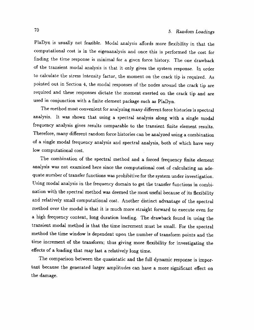
70 5. Random Loadings
PlaDyn is usually not feasible. Modal analysis affords more flexibility in that the
computational cost is in the eigenanalysis and once this is performed the cost for
finding the time response is minimal for a givcn force history. The one drawback
of the transient modal analysis is that it only gives the system response. In order
to calculate the stress intensity factor, the moment on the crack tip is required. As
pointed out in Section 4, the modal responses of the nodes around the crack tip are
required and these responses dictate the moment exerted on the crack tip and are
used in conjunction with a finite element package such as PlaDyn.
The method most convenient for analyzing many different force histories is spectral
analysis. It was shown that using a spectral analysis along with a single modal
frequency analysis gives results comparable to the transient finite element results.
Therefore, many different random force histories can be analyzed using a combination
of a single modal frequency analysis and spectral analysis, both of which have very
low computational cost.
The combination of the spectral method and a forced frequency finite element
analysis was not examined here since the computational cost of calculating an ade-
quate number of transfer functions was prohibitive for the system under investigation.
Using modal analysis in the frequency domain to get the transfer functions in combi-
nation with the spectral method was deemed the most useful because of its flexibility
and relatively small computational cost. Another distinct advantage of the spectral
method over the modal is that it is much more straight forward to execute even for
a high frequency content, long duration loading. The drawback found in using the
transient modal method is that the time increment must be small. For the spectral
method the time window is dependent upon the number of transform points and the
time increment of the transform; thus giving more flexibility for investigating the
effects of a loading that may last a relatively long time.
The comparison between the quasistatic and the full dynamic response is impor-
tant because the generated larger amplitudes can have a more significant effect on
the damage.
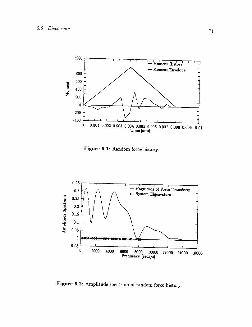
5.6 Discussion 71
1200
--Moment' I_" ' ' ''xstory
elope -800
600
400
2O0
0
-200
-400 I I I I t t i J I I I I I I I I l I I
0 0.001 0.002 0.003 0.004 0.005 0.006 0.007 0.008 0.009 0.01Time [secs]
Figure 5.1: Random force history.
0.35
0.3
-_ 0.25L_
0.2
0.15
'_- 0.1
"= 0.05
0
-0.050
I I I I I I I
-- Magnitude ofForce Transform
l I I t I I [
2000 4000 6000 8000 10000 12000 14000 16000Frequency [rads/s]
Figure 5.2: Amplitude spectrum of random force history.
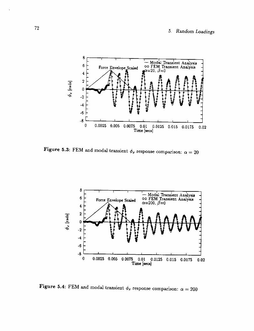
72 5. Random Loadings
"W
6
4
2
0
-2
-4
-6
-80
- -- Mo_
- Force Envelo-e Scaled oo FEM Transient Analysis --- __. , "-- .
__L._.__._ j L _
0.0025 0.005 0.0075 0.01 0.0125 0.015 0.0175 0.02Time [secs]
Figure 5.3: FEM and modal transient _. response comparison: a = 20
t_
-O-
4
2
0
-2
-4
-6
-8
Fo............ _ oo FEM^Traasient Analysisroe r,nvelope acateu Or=200 :_=0
0 0.0025 0.005 0.0075 0.01 0.0125 0.015 0.0175 0.02Time [secs]
Figure 5.4: FEM and modal transient ff_ response comparison: a = 200
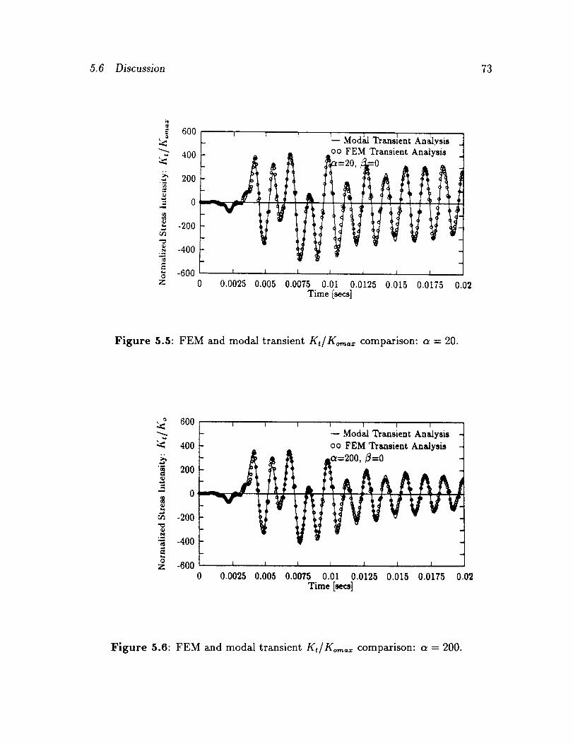
5.6 Discussion 73
600
400200
0
-200
-400
-600z
I
0 0.0025 0.005
oo FEM TransientAnalysis ._
.L l .L l
0.0075 0.01 0.0125 0.015 0.0175Time [secs]
0.02
Figure 5.5: FEM and modal transient Kt/Ko,,,°x comparison: a = 20.
° 600
_, 400200
0
i -200-400
z -600
r _ r T "r--_- -- Modal TransientAnalysis -
- oo FEM TransientAnalysis -
- -. .... .
0.0025 0.005 0.00?5 0.01 0.0125 0.015 0.0175 0.02Time [secs]
Figure 5.6: FEM and modal transient KJKo,,,,x comparison: a = 200.
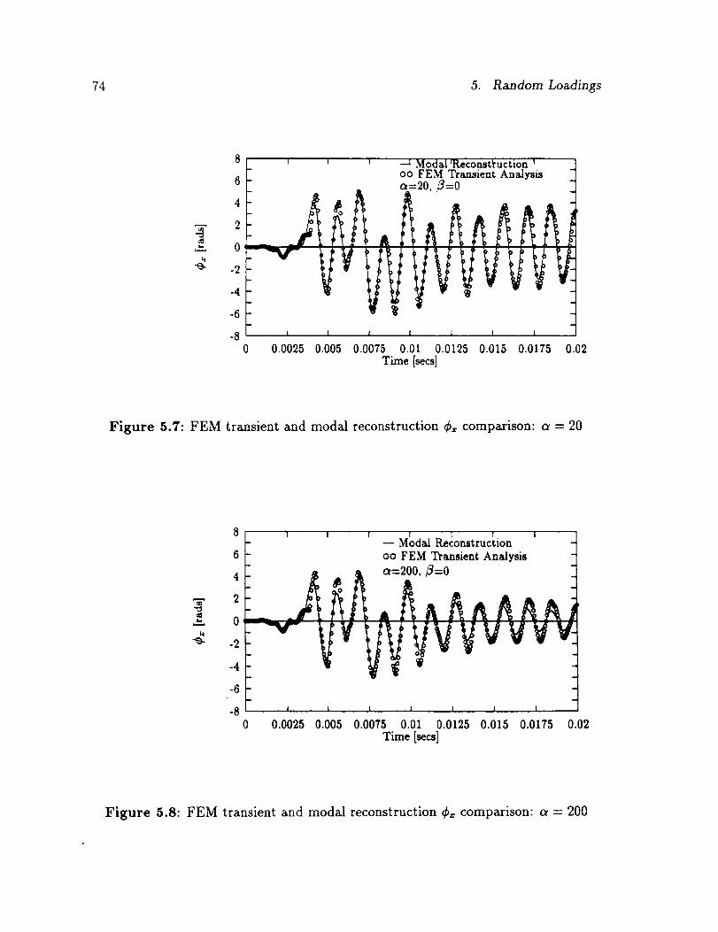
74 5. Random Loadings
.=_
4
2
0
-2
-4
-6
-80
r r T o a const uctlon
oo FEM TransientAnalysisa:20, 3=0
0.0025 0.005 0.0075 0.01 0.0125 0.015 0.0175 0.02Time [secs]
Figure 5.7: FEM transient and modal reconstruction ¢= comparison: a = 20
-,,j
6
4
2
0
-2
-4
-6
-8
I I I I [ I I
a=200,8=0- vvvvvv I [ I I I I I
0 0.0025 0.005 0.0075 0.01 0.0125 0.015 0.0175 0.02Time [secs]
Figure 5.8: FEM transient and modal reconstruction ¢= comparison: a = 200
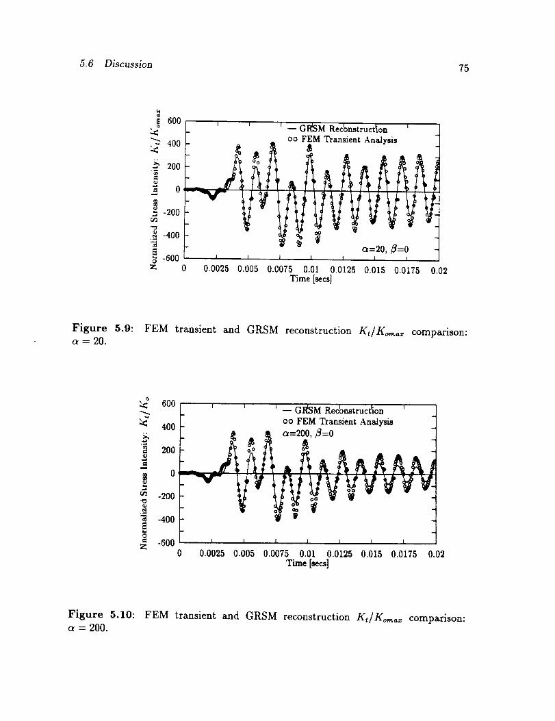
5.6 Discussion 75
N
60O
,_ 400
200
0
-200-400
- oo FEM Transient Analysis
- -a=20, _=0 -
Z 0 0.0025 0.005 0.0075 0.01 0.0125 0.015 0.0175 0.02Time [secs]
Figure 5.9: FEM transient and GRSM reconstruction KdKo,,,,, = comparison:a = 20.
600
400
'-_ 200
--_ 0
-200
.4
I 3"_ _ G M Reconstructon r
oo FEM TransientAnalysis
= -600 __.L _0 0.0025 0.005 0.0075 0.01 0.0125 0.015 0.0175 0.02
Time [secs]
Figure 5.10: FEM transient and GRSM reconstruction Kt/Ko_= comparison:a = 200.
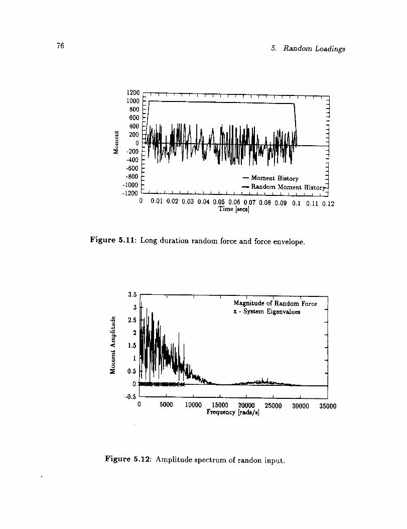
76 5. Random Loadings
1200
I000800
600
400- 200i°
-200
-400-600
-800-1000
-12000
_r---r--r--T__
L______
Moment lqistory
-- Random Moment History
0.01 0.02 0.03 0.04 0.05 0.06 0.07 0.08 0.09 0.I 0.ii 0.12Time [semi
Figure 5.11: Long duration random force and force envelope.
2K.v.,,] f , , l , ,
[a MagnitudeofRandom Force
3 _" [ ! x- System Eigenvalues
1.
i
0.5_0 _
-0.5 J x j l
0 5000 10000 15000 20000 25000 30000Frequency[fads/s]
35000
Figure 5.12: Amplitude spectrum of randon input.

5.6 Discussion 77
50
40
30
20
I0
0
-i0
-20
-30
-40
-500 0.01 0.02 0.03 0.04 0.05 0.06 0.07 0.08 0.09 0.i
Time [sees]
Figure 5.13: Modal and transient and modal reconstruction ¢= comparison: a = 20
40
30
20
0
-o- -10
-20
-30
-40
-50
0 0.01 0.02 0.03 0.04 0.05Time [sees]
Figure 5.14: Modal transient and modal reconstruction ¢_ comparison: expandedscale.
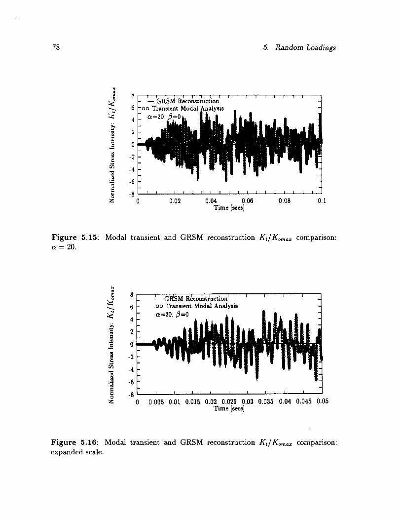
78 5. Random Loadings
8
6
4
._ 2
= 0
-2.=
_n -4
"- -6
=,'_ -87
t l I 1 i l I I I ] I 1 I I I I ] I I I /-- GRSM Reconstructionoo Transient Modal Analysisa=20,
0 0.02 0.04 0.06 0.08 0.ITime [secs]
Figure 5.15: Modal transient and GRSM reconstruction Kt/Ko_,.:_ comparison:
a=20.
8
6
4
= 0
] -2m -4
"_ -6
.=-8
Z
'-- GI_SM Rclcoustrluction'
oo TransientModal Analysis
a=20, _=0
! I I I
0 0.005 0.01 0.015 0.02 0.025 0.03 0.035 0.04 0.045 0.05
Time [_:s]
Figure 5.16: Modal transient and GRSM reconstruction Kt/Ko,-,,a= comparison:
expanded scale.
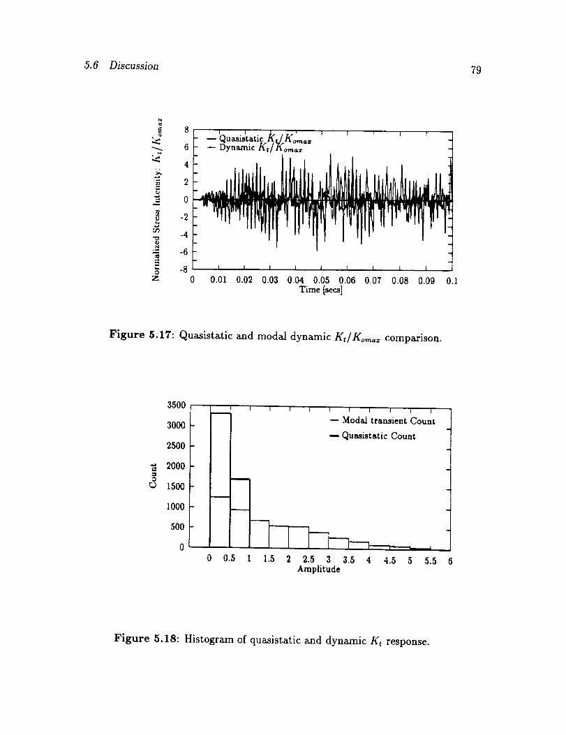
5.6 Discussion 79
z
i ! I l'!-4
-6
__ / I t l I I 1 I I
0 0.01 0.02 0.03 0.04 0.05 0.06 0.07 0.08 0.09 0.1Time [sees]
Figure 5.17: Quasistatic and modal dynamic Kt/Ko,_,_= comparison.
3500
3000
2500
2000
1500
I000
500
0
Ill
0 0.5 1.5 2 2.5 3 3.5 4 4.5 5 5.5 6Amplitude
Figure 5.18: Histogram of quasistatic and dynamic Kt response.

80 5. Random Loadings
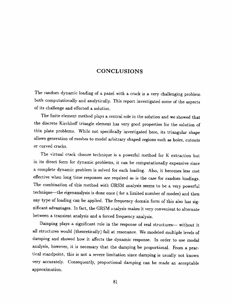
CONCLUSIONS
The random dynamic loading of a panel with a crack is a very challenging problem
both computationally and analytically. This report investigated some of the aspects
of its challenge and effected a solution.
The finite element method plays a central role in the solution and we showed that
the discrete Kirchhoff triangle element has very good properties for the solution of
thin plate problems. While not specifically investigated here, its triangular shape
allows generation of meshes to model arbitrary shaped regions such as holes, cutouts
or curved cracks.
The virtual crack closure technique is a powerful method for K extraction but
in its direct form for dynamic problems, it can be computationally expensive since
a complete dynamic problem is solved for each loading. Also, it becomes less cost
effective when long time responses are required as is the case for random loadings.
The combination of this method with GRSM analysis seems to be a very powerful
technique---the eigenanalysis is done once ( for a limited number of modes) and then
any type of loading can be applied. The frequency domain form of this also has sig-
nificant advantages. In fact, the GRSM aaalysis makes it very convenient to alternate
between a transient analysis and a forced frequency analysis.
Damping plays a significant role in the response of real structures-- without it
all structures would (theoretically) fail at resonance. We modeled multiple levels of
damping and showed how it affects the dynamic response. In order to use modal
analysis, however, it is necessary that the damping be proportional. From a prac-
tical standpoint, this is not a severe limitation since damping is usually not known
very accurately. Consequently, proportional damping can be made an acceptable
approximation.
81
82Conclusions
For a random loading, it was shown that it is vital to consider the dynamics of the
structure since multiple resonances may be spanned. Therefore, design should not
be based on the quasistatic results since they significantly underestimate the actual
response of the structure and hence the damage accumulation. This conclusion is
based on the results found in using Paris' equation for calculating crack growth. A
large difference between the quasistatic and the dynamic analysis was shown indicat-
ing that a dynamic analysis need be performed using one of the methods outlined
here. The particular method used to perform the analysis would depend upon the
problem specifications and requirements.
This research can now form the basis for the modeling of such difficult problems
as the effect of random loading on the fatigue growth in structures.
References
[1]
[2]
[3]
[4]
[5]
[6]
[7]
[8]
[9]
[lO]
[11]
[12]
[13]
Barsom, J.M., "Fatigue-Crack Propagation in Steels of Various Yield Strengths",Trans. ASME, J. Eng. Ind.,, vol. B73, No. 4, Nov 1971.
Batoz, J.L., Bathe, J.L., and Ho, L.W., "A Study of Three-Node Triangular
Plate Bending Elements", International Journal for Numerical Methods, vol. 15 pp.1745-1750, Jan 1980.
Cook, R.D., Concepts and Applications of Finite Element Analysis, John Wiley andSons, New York., 1989.
Doyle, J.F., Wave Propagation in Structures: An FFT-Based Spectral AnalysisMethodology, Kluwer Publishing, Boston, MA., 1989.
Doyle, J.F., Static and Dynamic Analysis of Structures, Kluwer Publishing, Boston,MA., 1991.
Dym, R. and Shames, R., Energy and Finite Element Methods in Structural Me-chanics, Hemisphere, Washington., 1985.
Irwin, G.R., "Fracture", Handbuch der Physic, vol. 6 pp. 551, Jan 1958.
Kanninen, M.F. and Popelar, C.H., Advanced Fracture Mechanics, Oxford Uni-versity Press, New York., 1985.
Kobayashi, A.S., Experimental Techniques in Fracture Mechanics, Iowa State Uni-versity Press, Ames, Iowa., 1973.
Leissa, A.W., Vibration of Plates, Scientific and Techncial Information Division;
Office of Tecnology and Utilization; National Aeronautics and Space Administration,Washington, D.C., 1969, 1969.
ModDyn, "Modal Analysis of Dynamic Systems", ikayex Software Tools, Lafayette,IN., 1992.
Petyt, M., Introduction to Finite Element Vibration Analysis, Oxford UniversityPress, New York., 1990.
PlaDyn, "A Program for the Static and Dynamic Analysis of Folded Plates", ikayezSoftware Tools, Lafayette, IN., 1992.
83
84 References
[14]
[15]
Rizzi, S.A., "A Frequency Based Approach to Dynamic Stress Intensity Analysis",
American Institute of Aeronautics and Astronautics Journal, pp. 2677-2683, 1991.
Rizzi, S.A., and Doyle, J.F., "Frequency Domain Stress Intensity Calibration of
Damped Cracked Panels", International Journal of Fracture, vol. 7 pp. 180-181, Sep1990.
[16]
[17]
[18]
[19]
Rolfe, S.T. and Barsom, J.M., Fracture and Fatigue Control in Structures, Pren-tice Hall, New Jersey., 1977.
Rook, D.P. and Cartwright, D.J., Compendium of Stress Intensity Factors,H.M.S.O., London., 1976.
Rybicki, E.R. and Kanninen, M.F., "A Finite Element Calculation of Stress In-
tensity Factors by a Modified Crack Closure Integral", Engineering Fracture Mechanics,vol. 9 pp. 931-938 1977.
Sih, G.C. and Paris, P.C. and Erdogan, F, "Crack Tip, Stress-Intensity Factors
for Plane Extension and Plate Bending Problems", Journal of Applied Mechanics,ASME 29, pp. 306-312 June 1962.
[20]
[21]
[22]
Stricklin, J.A., Haisler W., Tisdale, R., and Gunderson, R., "A Rapidly
Converging Triangular Plate Element ", American Institute o/Aeronautics and Astro-
nautics, vol. 7 pp. 180-181, Sep 1968.
Timoshenko, S. and Woinowsky-Krieger, S., Theory of Plates and Shells,McGraw-Hill, New York., 1959.
Wu, W-F, "Computer Simulation and Reliability Analysis of Fatigue Crack Propa-
gation Under Random Loading", Journal of Fracture Mechanics, vol. 45 pp. 697-712,Aug 1993.
[23] Young, M.J. Analysis of Cracked Plates Subjected to Out-Of-Plane Loadings. PhDthesis, Purdue University, 1991.
Times®-Roman
Times-BoldTimes-Italic
T'tmes-Boldltalic
ITC Avant Garde®-BookITC Avant Garde-Demi
ITC Avant Garde-BookObliqueITC Avant Garde-DemiOblique
Helvetica®-Narrow
Helvetica-Narrow-Bold
Helvetica-Narrow-ObliqueHelvetica-Narrow-BoldOblique
QMS-PS 810Version 47.2C
Defined Font Outlines
Helvetica ®Helvetica-Bold
Helvetica-ObliqueHelvetica-BoldOblique
Palatino®-RomanPalatino-BoldPalatir_Italic
Palatino-Boldltalic
ITC Zapf Chancery_-Mediumltalic
ITC Zapf Dingbats ®Symbols Set
CourierCourier-Bold
Courier,ObliqueCourier-BoldOblique
New Century Schoolbook-RomanNew Century Schoolbook-BoldNew Century Schoolbook-Italic
New Century Schoolbook-Boldltalic
ITC Bookman®.LightITC Bookman-Demi
ITC Bookrnan-Lighfltalic1TC Bookman-DcmLltalic
Times, He.lveer._ sod P_tinO am re_=ed mdmmks ot Linaqq_ Company.
ITC Avam _ ITC Zal_'C_mcery. rrc Za_ Disbars, msd 1.rc Booknun m _ _ __ T_ _