Fatigue in Aluminum Highway Bridges under Random Loading · 2015-01-20 · Fatigue in Aluminum...

International Journal of Applied Science and Technology Vol. 4, No. 6; November 2014

95

Fatigue in Aluminum Highway Bridges under Random Loading

Søren Rom MSc Eng.

Bridges, COWI A/S DK-2800 Lyngby, Denmark

Henning Agerskov Professor emeritus

Dept. of Civil Engrg. Tech. Univ. of Denmark

DK-2800 Lyngby, Denmark Abstract

Fatigue damage accumulation in aluminum highway bridges under random loading is studied. The fatigue life of welded joints has been determined both experimentally and from a fracture mechanics analysis. In the experimental part of the investigation, fatigue test series on welded plate test specimens have been carried through. The material that has been used has a 0.2% proof strength of 310 MPa and an ultimate tensile strength of 327 Mpa. The fatigue tests have been carried out using load histories, which correspond to one week’s traffic loading, determined by means of strain gauge measurements on the deck structure of the Farø Bridges in Denmark. The test series carried through show a significant difference between constant amplitude and variable amplitude fatigue test results. Both the fracture mechanics analysis and the fatigue test results indicate that Miner’s rule, which is normally used in the design against fatigue in aluminum bridges, may give results which are unconservative. The validity of the results obtained from Miner’s rule will depend on the distribution of the load history in tension and compression.

Keywords: Aluminum, Bridges, Highway bridges, Fatigue, Fatigue tests, Random processes

1. Introduction

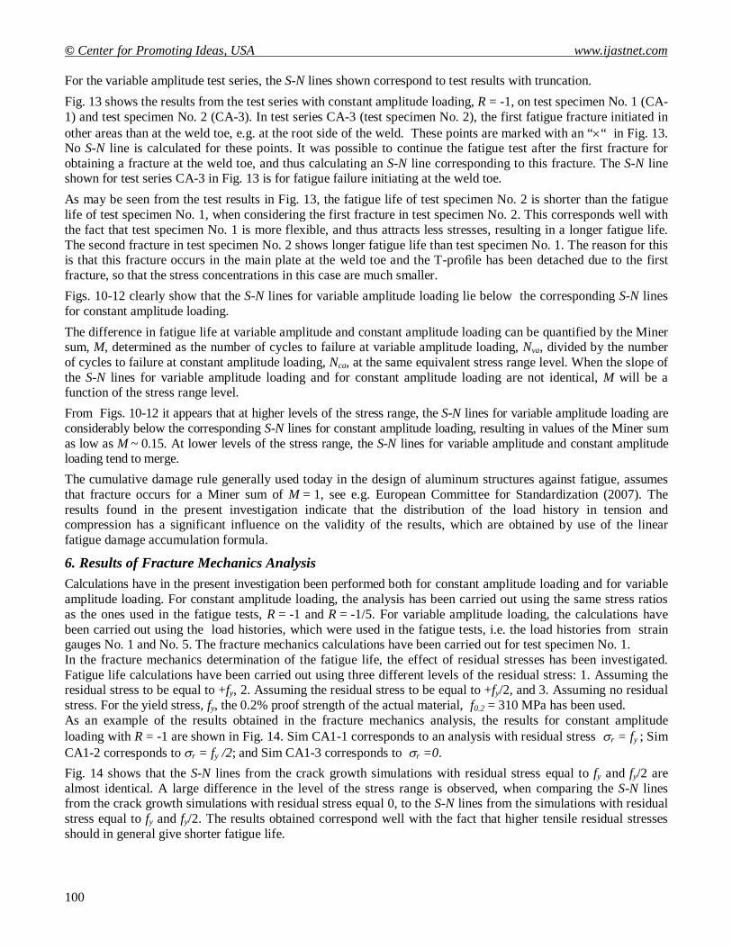
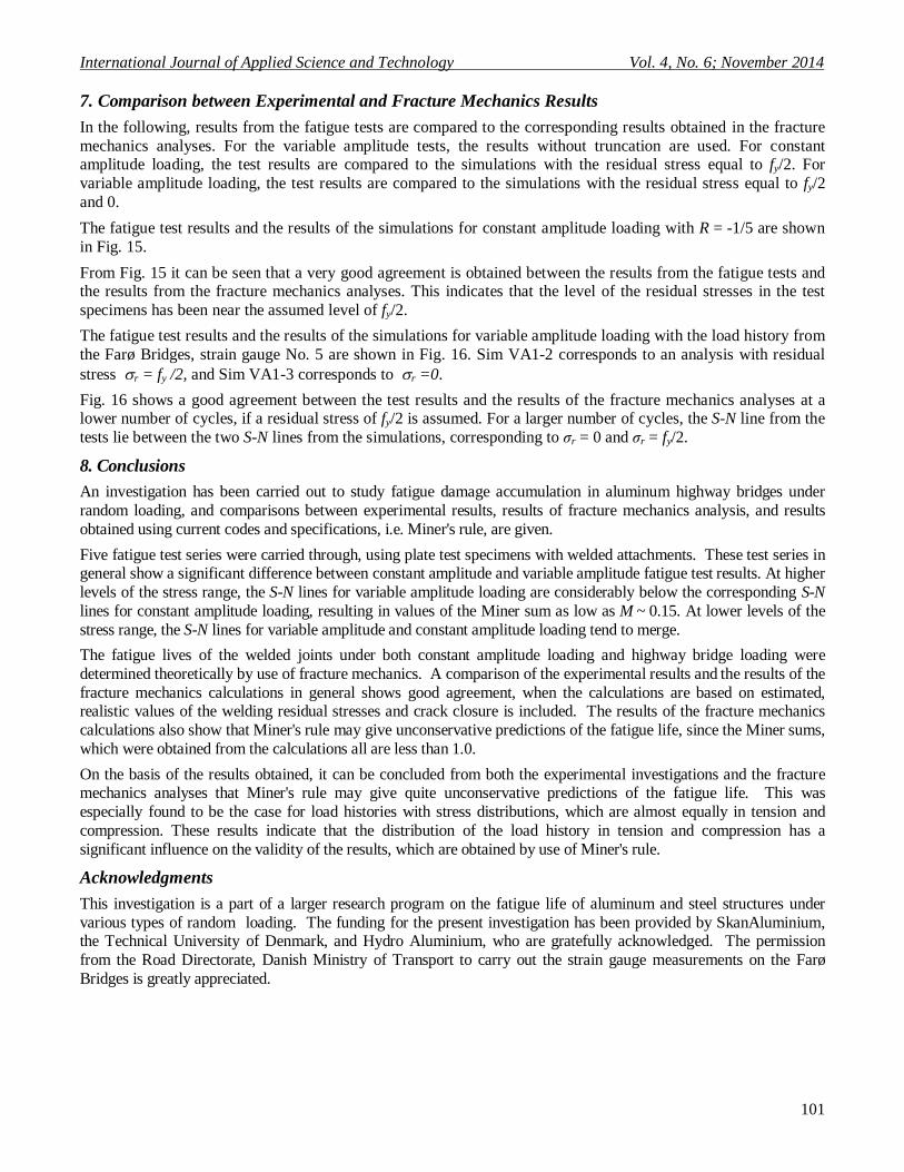
Aluminum is a relatively new material in permanent bridge structures. Aluminum is most commonly used for relatively small bridges, e.g. footbridges and short span road bridges. The low weight is one of the major advantages of aluminum in bridge structures, compared to the other bridge structure materials. Normally, specially developed extruded deck profiles are used in aluminum bridges. By welding the deck profiles together at the top and bottom flanges, an almost ideal isotropic bridge deck structure may be obtained. The deck profiles may be placed either in the longitudinal or transverse direction of the bridge. The choice of direction will depend on the bridge geometry and the way of construction. Main disadvantages in using aluminum for bridge structures are the low modulus of elasticity and the low fatigue strength, compared to steel. Fig.1 shows an example of an extruded aluminum profile for use in bridge deck structures, and Fig.2 an example of an aluminum bridge in Norway.

A major concern in the design of aluminum bridges is the fatigue life. One of the problems that have attracted increased attention in recent years is the problem of fatigue damage accumulation. Codes and specifications normally give simple rules, using a Miner summation and based on the results of constant amplitude fatigue tests. Over the years, fatigue test series have been carried through using different types of block loadings, and for these types of loading, Miner's rule has in many cases been found to give reasonable results. However, in a real structure the loading does normally not consist of loading blocks, but the structure is subjected to a stochastic loading, due to traffic, wind, etc. Thus, the need for a better understanding of the fatigue behavior under more realistic fatigue loading conditions is obvious. The question of the validity of Miner's rule has been the background for a series of research projects on fatigue in aluminum and steel structures, carried out at the Department of Civil Engineering of the Technical University of Denmark over a long period of time.

© Center for Promoting Ideas, USA www.ijastnet.com

96

The primary purpose of these projects has been to study the fatigue life of aluminum and steel structures under various types of stochastic loading that are realistic in relation to these types of structures. This paper concentrates on the results of the investigations on aluminum bridges.

The types of loading that are used in the present investigation correspond to one week's traffic loading, determined by means of strain gauge measurements at various locations in the deck structure of the Farø Bridges in Denmark. The fatigue tests have been carried out on welded plate test specimens.

Besides the fatigue tests, the present investigation also includes analytical determination of the fatigue life under the actual types of random loading by use of fracture mechanics, to be able to compare experimentally and theoretically determined fatigue lives.

2. Experimental Investigation

2.1 Test Specimens

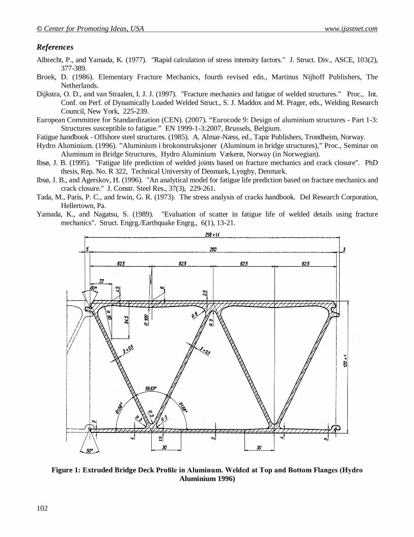
In the experimental investigation, two types of welded test specimens have been used. Test specimen No. 1 consists of a special extruded profile which is welded to the main plate of the test specimen. This test specimen is shown in Fig. 3. Test specimen No. 2 consists of a traditional extruded T-profile welded to the main plate of the test specimen, see Fig. 4. Test specimen No. 1 is intended to give lower stress concentration at the weld toe than test specimen No. 2.

The material used for the test specimens is Al 6005 T6. The ultimate tensile strength and the 0.2% proof strength for the test specimens were determined to be: fu = 327 MPa and f0.2 = 310 MPa, respectively. Both profiles used are extruded and both are welded to a main plate of width 400 mm and thickness 10 mm. The individual test specimens are then fabricated by sawing in pieces of width 45 mm.

2.2 Test Equipment and Test Procedures

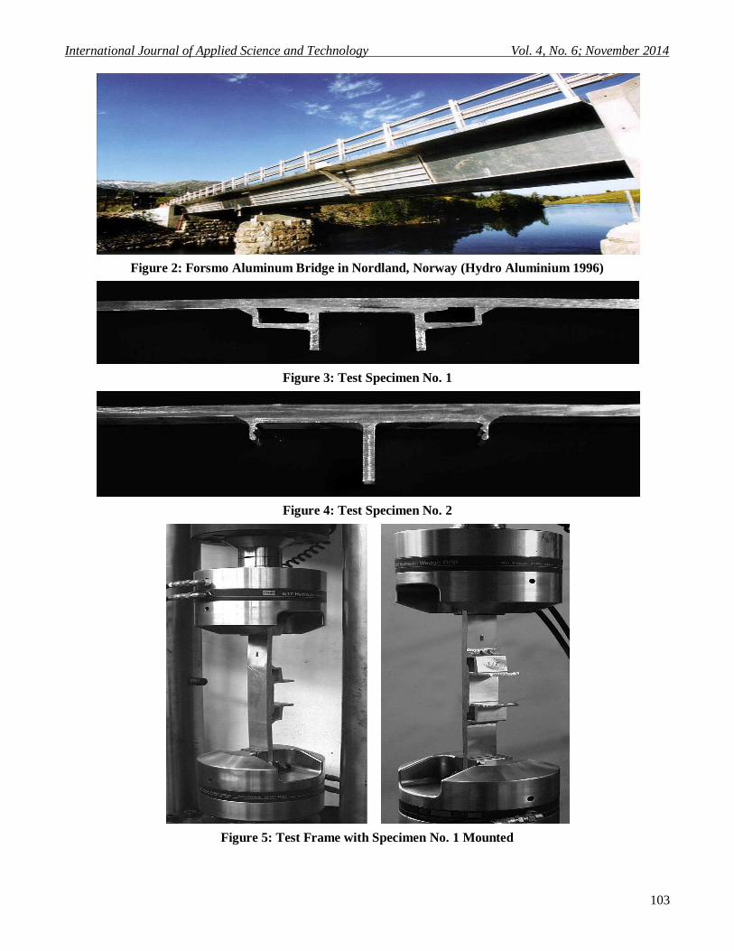
The fatigue tests have been carried out in a fixed test frame with a capacity of ±100 kN. The applied loading in these tests is a central normal force in the main plate. Small eccentricities due to the welding of the test specimens are inevitable in these test series. This results in additional secondary bending stresses at the joint. Strain gauges are used on all test specimens in these series to determine the resulting stresses from normal force and eccentricity moment. Furthermore, the stresses in the most critical areas with respect to fatigue have been determined from finite element analysis. Fig. 5 shows the test frame used with test specimen No. 1 mounted. Both constant amplitude and variable amplitude fatigue tests are included in the present investigation. For the variable amplitude tests, the load sequence is controlled by a computer, reading from a file containing the load history. The computer sends the load sequence to the servo-controller of the test equipment.

During the fatigue test, sequences of peak values from the strain measurements are read. In the case of constant amplitude tests, only few readings are needed to determine the stress range, while longer sequences, corresponding to the length of the load histories, are needed in the tests with variable amplitude loading to get a reliable equivalent stress range from the rainflow counting on the stress history.

3. Variable Amplitude Loading

The variable amplitude loading that has been used in the fatigue tests of the present investigation has been deter-mined from strain gauge measurements on the steel deck structure of the Farø Bridges in Denmark. No similar stress histories measured on aluminum bridges were found at the start of this investigation. The load histories correspond to one week's traffic loading. Strain gauge measurements were taken at 10 different locations in the deck structure. The load histories that have been used in the present investigation were measured by two strain gauges, both placed on the bottom of one of the trapezoidal longitudinal stiffeners of the deck plate. The stiffener chosen is located under the most heavily loaded lane of the motorway. The distance from the measurement area to the simple support of the bridge girder on the nearest bridge pier is approximately 8 m. With a length of the bridge spans of approximately 80 m, this location of the strain gauges means that only local bending effects in the deck structure will be registered, whereas the stresses due to global bending in the bridge girder will be negligible. Strain gauge No. 1 is placed in the middle of the longitudinal stiffener span, which has a length of 4 m. Strain gauge No. 5 is placed at a distance of 0.5 m from one of the transverse diaphragms. This means that the stresses measured by strain gauge No. 1 are primarily tensile stresses, whereas the stresses registered by strain gauge No. 5 are almost equally in tension and compression.


97

Only the extremes of the load history are needed, since the load course between consecutive extremes is considered unimportant. Thus, only the peak values of the stress history, registered by the strain gauges during the measuring period, are stored in the computer.

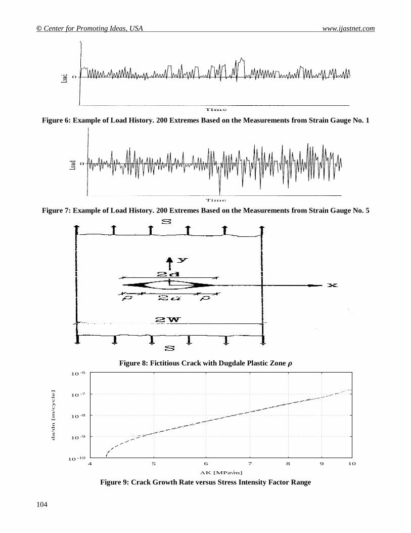
In order to avoid noise and low, non-damaging stress cycles in the stress history to be used in the fatigue tests, a truncation is carried out on the directly registered stress history. The truncation level th has been determined by use of linear elastic fracture mechanics, on the basis of a choice of the threshold value of the stress intensity factor range, Kth = 4.2 mMPa . This value was determined from crack growth measurements on the material used. Figs. 6 and 7 show examples of typical load histories based on the measurements from strain gauges No. 1 and 5, respectively. The load level in each variable amplitude test is determined from the measured load history by multiplication with a scaling factor. The frequency used in the tests is 10-30 cycles per second. When the load history corresponding to one week's traffic has been simulated in the fatigue test, the simulation procedure returns to the beginning of the load history and repeats the one week loading.

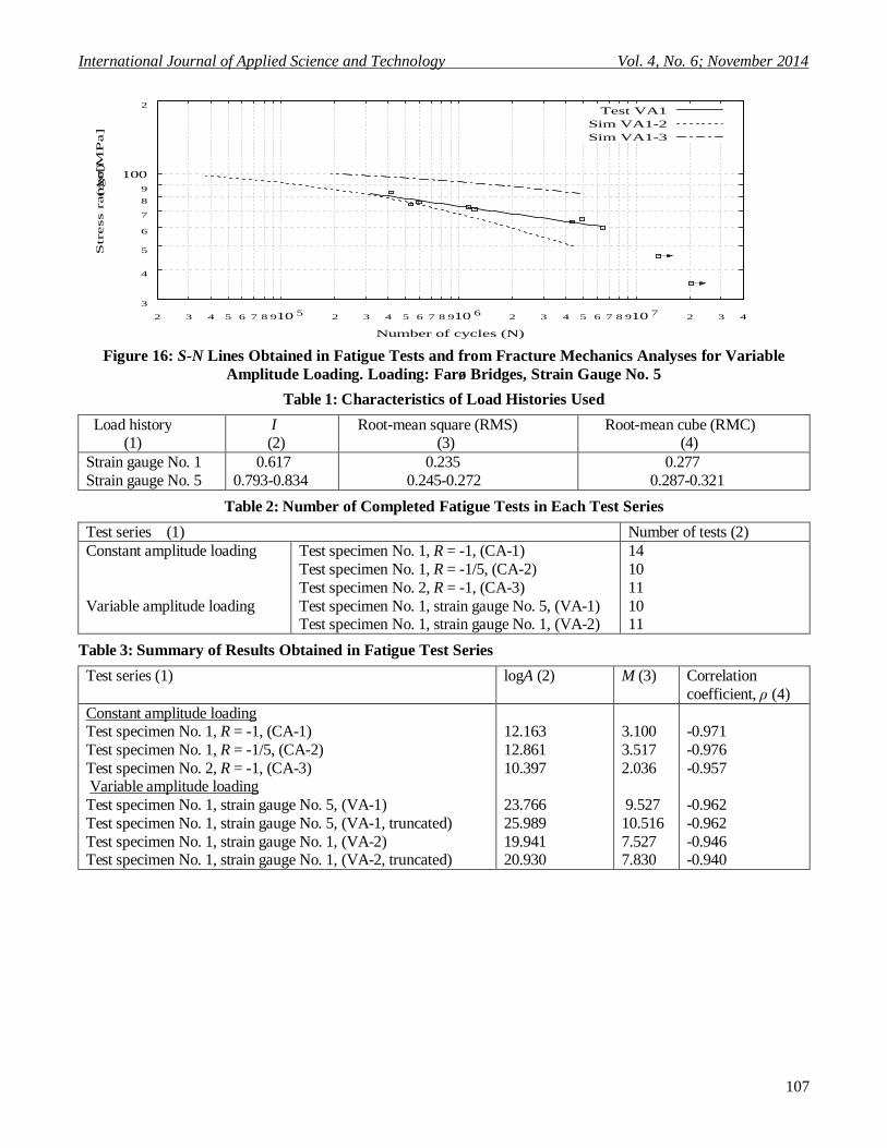
The main characteristics of the load histories based on the measurements from strain gauges No. 1 and 5 are given in Table 1. The irregularity factor, I, is defined as the number of positive-going mean-value crossings divided by the number of maxima of the load history. For narrow band loading, the irregularity factor will be close to unity. Root-mean-square (RMS) and root-mean-cube (RMC) values have been determined from rainflow counts on the load histories. The RMS- and RMC-values given in Table 1 correspond to a maximum stress range in the stress history, max = 1.

4. Fracture Mechanics Prediction of Fatigue Life

The fatigue life of welded joints can be determined theoretically by the use of fracture mechanics. Of special importance for the validity of the results that are obtained from the fracture mechanics analysis is the consideration of crack closure in the analytical model.

The crack growth analysis model used in the present investigation is based on the Dugdale-Barenblatt strip yielding assumption, with modifications to allow plastically deformed material to be left along the crack surfaces as the crack grows. The crack closure model accounts for load interaction effects, such as retardation and acceleration, under variable amplitude loading. The model may be used to simulate fatigue crack growth under both constant amplitude and variable amplitude loading taking into account the influence of crack closure upon fatigue crack growth. Furthermore, in the determination of the crack growth life the effects of stress concentrations and welding residual stresses are included. In the following is given a brief description of the crack growth model and of the most important parameters used in the model. The present paper concentrates on the experimental investigations, and thus only a short mention of the results of the fracture mechanics calculations is included.

The mechanisms of crack closure have been attributed to plasticity-induced closure, roughness-induced closure and environment-induced closure. Only the plasticity-induced closure is included in the crack closure model used in the present investigation.

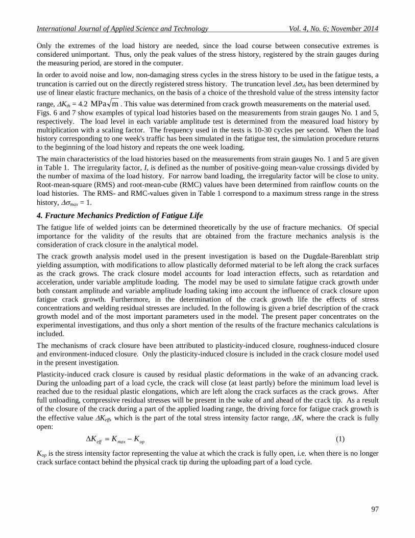
Plasticity-induced crack closure is caused by residual plastic deformations in the wake of an advancing crack. During the unloading part of a load cycle, the crack will close (at least partly) before the minimum load level is reached due to the residual plastic elongations, which are left along the crack surfaces as the crack grows. After full unloading, compressive residual stresses will be present in the wake of and ahead of the crack tip. As a result of the closure of the crack during a part of the applied loading range, the driving force for fatigue crack growth is the effective value Keff, which is the part of the total stress intensity factor range, K, where the crack is fully open:

opmaxeff KKK (1)

Kop is the stress intensity factor representing the value at which the crack is fully open, i.e. when there is no longer crack surface contact behind the physical crack tip during the uploading part of a load cycle.


98

The fatigue crack growth rate may be presumed to follow a power law of the following form:

theffeff

theffeffm

theffmeff

KKdnda

KKKKCdnda

,

,,

for0

for)(

(2)

where Keff,th is the effective threshold stress intensity factor range, below which no crack growth takes place, considering the effect of crack closure.

A fictitious crack with half length d, where d=a+, is used in the model. a is half the physical crack length, and is the length of the plastic zone. Fig. 8 shows the fictitious crack with half length d.

In the calculations of the fatigue life using the crack closure model, the following assumptions have been made: 1) only one semi-elliptical crack is growing in the plate element; 2) the ratio between the semi-axes of the crack, a/b, is constant throughout the calculation; 3) as an approximation for taking strain hardening into consideration, the flow stress o, which is the average value of the yield stress, fy (the 0.2% proof strength, f0.2), and the ultimate tensile strength, fu, is introduced; and 4) plane stress and plane strain conditions, as well as conditions between these two, are simulated by using a constraint factor on the tensile yielding at the crack front to approximately account for three-dimensional stress states.

A widely used approximate calculation of the stress intensity factor for a surface semi-elliptical crack in a structural detail is obtained by using the method proposed by Albrecht and Yamada (1977). Using this method, K is expressed as follows:

aSFFFFK GTES (3)

where FS, FE, FT and FG are correction factors for free surface, elliptical crack shape, finite plate thickness or width, and geometry or stress gradient, respectively. The stress intensity factor corrections, FS, FE, and FT may be found from Tada, Paris, and Irwin (1973), Albrecht and Yamada (1977), Fatigue Handbook (1985) and Broek (1986). FG may be determined from the results of a finite element analysis using the weight function method. S is the remote applied stress.

The crack growth coefficients, m and C, in Eq. 2 were determined from crack growth measurements carried out on standard Compact-Tension (CT) specimens. The actual values of m and C were determined by a linear regression of crack growth rate data using the method of least squares. The following values of m and C were obtained:

28.4m (4)

4.28

12

)m(MPam1048.4 C (5)

The measured crack growth rate as a function of the stress intensity factor range is shown in Fig. 9. Based on the results shown in Fig. 9, the effective threshold stress intensity factor range may be taken as

mMPa2.4, theffK (6)

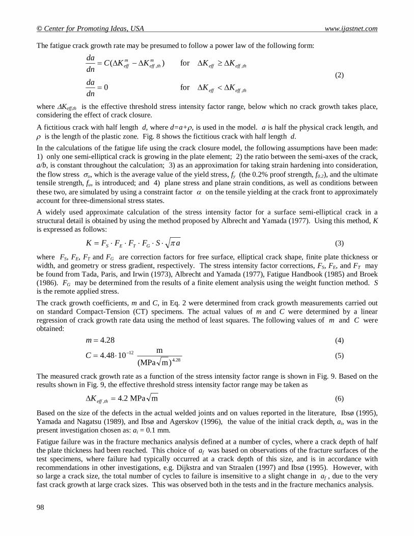
Based on the size of the defects in the actual welded joints and on values reported in the literature, Ibsø (1995), Yamada and Nagatsu (1989), and Ibsø and Agerskov (1996), the value of the initial crack depth, ai, was in the present investigation chosen as: ai = 0.1 mm.

Fatigue failure was in the fracture mechanics analysis defined at a number of cycles, where a crack depth of half the plate thickness had been reached. This choice of af was based on observations of the fracture surfaces of the test specimens, where failure had typically occurred at a crack depth of this size, and is in accordance with recommendations in other investigations, e.g. Dijkstra and van Straalen (1997) and Ibsø (1995). However, with so large a crack size, the total number of cycles to failure is insensitive to a slight change in af , due to the very fast crack growth at large crack sizes. This was observed both in the tests and in the fracture mechanics analysis.


99

Thus, with a plate thickness of 10 mm, the crack depth, af, corresponding to the final or critical crack size was chosen as: af = 5 mm. In the fatigue tests, the number of cycles to failure was defined as the number of cycles, where the test specimen actually broke.

5. Fatigue Test Results

In the following are given the results that have been obtained in the fatigue tests. Initial test series with constant amplitude loading were carried out as a reference, and also to obtain the actual value of the exponent m for calculation of the equivalent stress ranges of the tests with variable amplitude loading.

The load histories based on the measurements from strain gauge No. 5 are almost equally in tension and compression. Furthermore, the maximum stresses in tension and compression are practically the same for these load histories. This means that the results of the test series with the load histories based on strain gauge No. 5 should be compared with the constant amplitude test series with a stress ratio, R = -1.

The load history resulting from the measurements from strain gauge No. 1 is primarily in the tension area. It appears from the load history that approximately 5/6 of the stress is in tension and approximately 1/6 is in compression. Thus, it seems reasonable to compare the results obtained in this test series with the results from the constant amplitude test series with R = -1/5.

Five fatigue test series were carried through:

CA-1 Constant amplitude loading, R = -1, test specimen No. 1. VA-1 Variable amplitude loading, strain gauge No. 5, test specimen No. 1. CA-2 Constant amplitude loading, R = -1/5, test specimen No. 1. VA-2 Variable amplitude loading, strain gauge No. 1, test specimen No. 1. CA-3 Constant amplitude loading, R = -1, test specimen No. 2.

In Table 2, the number of tests carried out in each test series is given. Table 2 includes both the constant amplitude test series and the variable amplitude test series.

The results obtained in the test series with constant amplitude loading and in the series with bridge loading are shown in Figs. 10-13. In the results from the variable amplitude tests, the stress parameter used is the equivalent constant amplitude stress range, e, defined as:

m

imii

e Nn

/1)(

(7)

In which ni = number of cycles of stress range i; i = variable amplitude stress range; N = total number of cycles to failure (=ini); and m = slope of corresponding constant amplitude S-N line.

For the results obtained in each test series, the data are fitted to an expression:

logloglog mAN (8)

By the method of least squares. In Eq. 8, m and A are constants, N is the number of cycles to failure, and is the stress range.

In the S-N diagrams, points marked with an arrow correspond to a test with a non-broken test specimen. These points have not been included in the regression analysis.

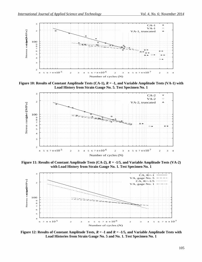
The results obtained in the test series on test specimen No. 1 under constant amplitude loading (CA-1) with stress ratio R = -1 and variable amplitude loading (VA-1) with the load history from strain gauge No. 5 are shown in the S-N diagram in Fig. 10. Fig. 11 shows the results that have been obtained in the test series on test specimen No. 1 under constant amplitude loading (CA-2) with stress ratio R = -1/5 and variable amplitude loading (VA-2) with the load history from strain gauge No. 1. For the variable amplitude tests in Figs. 10-11, the results are shown both with and without truncation.

The main data for the S-N lines obtained are summarized in Table 3.

The S-N diagram in Fig. 12 shows a comparison between the S-N lines obtained in the 4 test series on test specimen No. 1: CA-1, CA-2, VA-1 and VA-2.


100

For the variable amplitude test series, the S-N lines shown correspond to test results with truncation.

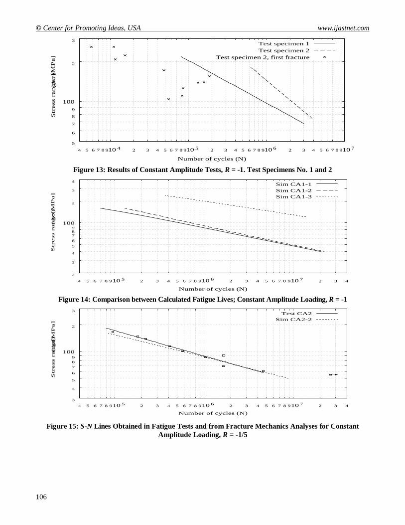
Fig. 13 shows the results from the test series with constant amplitude loading, R = -1, on test specimen No. 1 (CA-1) and test specimen No. 2 (CA-3). In test series CA-3 (test specimen No. 2), the first fatigue fracture initiated in other areas than at the weld toe, e.g. at the root side of the weld. These points are marked with an ““ in Fig. 13. No S-N line is calculated for these points. It was possible to continue the fatigue test after the first fracture for obtaining a fracture at the weld toe, and thus calculating an S-N line corresponding to this fracture. The S-N line shown for test series CA-3 in Fig. 13 is for fatigue failure initiating at the weld toe.

As may be seen from the test results in Fig. 13, the fatigue life of test specimen No. 2 is shorter than the fatigue life of test specimen No. 1, when considering the first fracture in test specimen No. 2. This corresponds well with the fact that test specimen No. 1 is more flexible, and thus attracts less stresses, resulting in a longer fatigue life. The second fracture in test specimen No. 2 shows longer fatigue life than test specimen No. 1. The reason for this is that this fracture occurs in the main plate at the weld toe and the T-profile has been detached due to the first fracture, so that the stress concentrations in this case are much smaller.

Figs. 10-12 clearly show that the S-N lines for variable amplitude loading lie below the corresponding S-N lines for constant amplitude loading.

The difference in fatigue life at variable amplitude and constant amplitude loading can be quantified by the Miner sum, M, determined as the number of cycles to failure at variable amplitude loading, Nva, divided by the number of cycles to failure at constant amplitude loading, Nca, at the same equivalent stress range level. When the slope of the S-N lines for variable amplitude loading and for constant amplitude loading are not identical, M will be a function of the stress range level.

From Figs. 10-12 it appears that at higher levels of the stress range, the S-N lines for variable amplitude loading are considerably below the corresponding S-N lines for constant amplitude loading, resulting in values of the Miner sum as low as M ~ 0.15. At lower levels of the stress range, the S-N lines for variable amplitude and constant amplitude loading tend to merge.

The cumulative damage rule generally used today in the design of aluminum structures against fatigue, assumes that fracture occurs for a Miner sum of M = 1, see e.g. European Committee for Standardization (2007). The results found in the present investigation indicate that the distribution of the load history in tension and compression has a significant influence on the validity of the results, which are obtained by use of the linear fatigue damage accumulation formula.

6. Results of Fracture Mechanics Analysis

Calculations have in the present investigation been performed both for constant amplitude loading and for variable amplitude loading. For constant amplitude loading, the analysis has been carried out using the same stress ratios as the ones used in the fatigue tests, R = -1 and R = -1/5. For variable amplitude loading, the calculations have been carried out using the load histories, which were used in the fatigue tests, i.e. the load histories from strain gauges No. 1 and No. 5. The fracture mechanics calculations have been carried out for test specimen No. 1. In the fracture mechanics determination of the fatigue life, the effect of residual stresses has been investigated. Fatigue life calculations have been carried out using three different levels of the residual stress: 1. Assuming the residual stress to be equal to +fy, 2. Assuming the residual stress to be equal to +fy/2, and 3. Assuming no residual stress. For the yield stress, fy, the 0.2% proof strength of the actual material, f0.2 = 310 MPa has been used. As an example of the results obtained in the fracture mechanics analysis, the results for constant amplitude loading with R = -1 are shown in Fig. 14. Sim CA1-1 corresponds to an analysis with residual stress r = fy ; Sim CA1-2 corresponds to r = fy /2; and Sim CA1-3 corresponds to r =0.

Fig. 14 shows that the S-N lines from the crack growth simulations with residual stress equal to fy and fy/2 are almost identical. A large difference in the level of the stress range is observed, when comparing the S-N lines from the crack growth simulations with residual stress equal 0, to the S-N lines from the simulations with residual stress equal to fy and fy/2. The results obtained correspond well with the fact that higher tensile residual stresses should in general give shorter fatigue life.


101

7. Comparison between Experimental and Fracture Mechanics Results

In the following, results from the fatigue tests are compared to the corresponding results obtained in the fracture mechanics analyses. For the variable amplitude tests, the results without truncation are used. For constant amplitude loading, the test results are compared to the simulations with the residual stress equal to fy/2. For variable amplitude loading, the test results are compared to the simulations with the residual stress equal to fy/2 and 0.

The fatigue test results and the results of the simulations for constant amplitude loading with R = -1/5 are shown in Fig. 15.

From Fig. 15 it can be seen that a very good agreement is obtained between the results from the fatigue tests and the results from the fracture mechanics analyses. This indicates that the level of the residual stresses in the test specimens has been near the assumed level of fy/2.

The fatigue test results and the results of the simulations for variable amplitude loading with the load history from the Farø Bridges, strain gauge No. 5 are shown in Fig. 16. Sim VA1-2 corresponds to an analysis with residual stress r = fy /2, and Sim VA1-3 corresponds to r =0.

Fig. 16 shows a good agreement between the test results and the results of the fracture mechanics analyses at a lower number of cycles, if a residual stress of fy/2 is assumed. For a larger number of cycles, the S-N line from the tests lie between the two S-N lines from the simulations, corresponding to σr = 0 and σr = fy/2.

8. Conclusions

An investigation has been carried out to study fatigue damage accumulation in aluminum highway bridges under random loading, and comparisons between experimental results, results of fracture mechanics analysis, and results obtained using current codes and specifications, i.e. Miner's rule, are given.

Five fatigue test series were carried through, using plate test specimens with welded attachments. These test series in general show a significant difference between constant amplitude and variable amplitude fatigue test results. At higher levels of the stress range, the S-N lines for variable amplitude loading are considerably below the corresponding S-N lines for constant amplitude loading, resulting in values of the Miner sum as low as M ~ 0.15. At lower levels of the stress range, the S-N lines for variable amplitude and constant amplitude loading tend to merge.

The fatigue lives of the welded joints under both constant amplitude loading and highway bridge loading were determined theoretically by use of fracture mechanics. A comparison of the experimental results and the results of the fracture mechanics calculations in general shows good agreement, when the calculations are based on estimated, realistic values of the welding residual stresses and crack closure is included. The results of the fracture mechanics calculations also show that Miner's rule may give unconservative predictions of the fatigue life, since the Miner sums, which were obtained from the calculations all are less than 1.0.

On the basis of the results obtained, it can be concluded from both the experimental investigations and the fracture mechanics analyses that Miner's rule may give quite unconservative predictions of the fatigue life. This was especially found to be the case for load histories with stress distributions, which are almost equally in tension and compression. These results indicate that the distribution of the load history in tension and compression has a significant influence on the validity of the results, which are obtained by use of Miner's rule.

Acknowledgments

This investigation is a part of a larger research program on the fatigue life of aluminum and steel structures under various types of random loading. The funding for the present investigation has been provided by SkanAluminium, the Technical University of Denmark, and Hydro Aluminium, who are gratefully acknowledged. The permission from the Road Directorate, Danish Ministry of Transport to carry out the strain gauge measurements on the Farø Bridges is greatly appreciated.


102

References

Albrecht, P., and Yamada, K. (1977). "Rapid calculation of stress intensity factors." J. Struct. Div., ASCE, 103(2), 377-389.

Broek, D. (1986). Elementary Fracture Mechanics, fourth revised edn., Martinus Nijhoff Publishers, The Netherlands.

Dijkstra, O. D., and van Straalen, I. J. J. (1997). "Fracture mechanics and fatigue of welded structures." Proc., Int. Conf. on Perf. of Dynamically Loaded Welded Struct., S. J. Maddox and M. Prager, eds., Welding Research Council, New York, 225-239.

European Committee for Standardization (CEN). (2007). “Eurocode 9: Design of aluminium structures - Part 1-3: Structures susceptible to fatigue.” EN 1999-1-3:2007, Brussels, Belgium.

Fatigue handbook - Offshore steel structures. (1985). A. Almar-Næss, ed., Tapir Publishers, Trondheim, Norway. Hydro Aluminium. (1996). ”Aluminium i brokonstruksjoner (Aluminum in bridge structures),” Proc., Seminar on

Aluminum in Bridge Structures, Hydro Aluminium Vækerø, Norway (in Norwegian). Ibsø, J. B. (1995). "Fatigue life prediction of welded joints based on fracture mechanics and crack closure". PhD

thesis, Rep. No. R 322, Technical University of Denmark, Lyngby, Denmark. Ibsø, J. B., and Agerskov, H. (1996). "An analytical model for fatigue life prediction based on fracture mechanics and

crack closure." J. Constr. Steel Res., 37(3), 229-261. Tada, M., Paris, P. C., and Irwin, G. R. (1973). The stress analysis of cracks handbook. Del Research Corporation,

Hellertown, Pa. Yamada, K., and Nagatsu, S. (1989). "Evaluation of scatter in fatigue life of welded details using fracture

mechanics". Struct. Engrg./Earthquake Engrg., 6(1), 13-21.

Figure 1: Extruded Bridge Deck Profile in Aluminum. Welded at Top and Bottom Flanges (Hydro Aluminium 1996)


103

Figure 2: Forsmo Aluminum Bridge in Nordland, Norway (Hydro Aluminium 1996)

Figure 3: Test Specimen No. 1

Figure 4: Test Specimen No. 2

Figure 5: Test Frame with Specimen No. 1 Mounted


104

Figure 6: Example of Load History. 200 Extremes Based on the Measurements from Strain Gauge No. 1

Figure 7: Example of Load History. 200 Extremes Based on the Measurements from Strain Gauge No. 5

Figure 8: Fictitious Crack with Dugdale Plastic Zone

Figure 9: Crack Growth Rate versus Stress Intensity Factor Range

10 -10

10 -9

10 -8

10 -7

10 -6

4 5 6 7 8 9 10

da/d

n [

m/c

ycle

]

K [MPam]


105

Figure 10: Results of Constant Amplitude Tests (CA-1), R = -1, and Variable Amplitude Tests (VA-1) with Load History from Strain Gauge No. 5. Test Specimen No. 1

Figure 11: Results of Constant Amplitude Tests (CA-2), R = -1/5, and Variable Amplitude Tests (VA-2) with Load History from Strain Gauge No. 1. Test Specimen No. 1

Figure 12: Results of Constant Amplitude Tests, R = -1 and R = -1/5, and Variable Amplitude Tests with Load Histories from Strain Gauge No. 5 and No. 1. Test Specimen No. 1

2

3

4

5

6789

100

2

3

4 5 6 7 8 910 5 2 3 4 5 6 7 8 910 6 2 3 4 5 6 7 8 910 7 2 3 4

Str

ess

ran

ge

[M

Pa]

Number of cycles (N)

CA-1VA-1

VA-1, truncated

2

3

4

5

6789

100

2

3

4 5 6 7 8 910 5 2 3 4 5 6 7 8 910 6 2 3 4 5 6 7 8 910 7 2 3 4

Str

ess

ran

ge[M

Pa]


CA-2VA-2

VA-2, truncated

4

5

6

7

89

100

2

3

6 7 8 9 10 5 2 3 4 5 6 7 8 9 10 6 2 3 4 5 6 7 8 9 10 7

Str

ess r

an

ge

[M

Pa]


CA, R=-1VA, gage No. 5

CA, R=-1/5VA, gage No. 1


106

Figure 13: Results of Constant Amplitude Tests, R = -1. Test Specimens No. 1 and 2

Figure 14: Comparison between Calculated Fatigue Lives; Constant Amplitude Loading, R = -1

Figure 15: S-N Lines Obtained in Fatigue Tests and from Fracture Mechanics Analyses for Constant Amplitude Loading, R = -1/5

5

6

7

8

9

100

2

3

4 5 6 7 8 910 4 2 3 4 5 6 7 8 910 5 2 3 4 5 6 7 8 910 6 2 3 4 5 6 7 8 910 7

Str

ess

ran

ge

[M

Pa]


Test specimen 1Test specimen 2

Test specimen 2, first fracture

2

3

4

56789

100

2

3

4

4 5 6 7 8 910 5 2 3 4 5 6 7 8 910 6 2 3 4 5 6 7 8 910 7 2 3 4

Str

ess

ran

ge

[M

Pa]


Sim CA1-1Sim CA1-2Sim CA1-3

3

4

5

6

789

100

2

3

4 5 6 7 8 910 5 2 3 4 5 6 7 8 910 6 2 3 4 5 6 7 8 910 7 2 3 4

Str

ess r

an

ge

[M

Pa]


Test CA2Sim CA2-2


107

Figure 16: S-N Lines Obtained in Fatigue Tests and from Fracture Mechanics Analyses for Variable

Amplitude Loading. Loading: Farø Bridges, Strain Gauge No. 5

Table 1: Characteristics of Load Histories Used

Load history (1)

I (2)

Root-mean square (RMS) (3)

Root-mean cube (RMC) (4)

Strain gauge No. 1 Strain gauge No. 5

0.617 0.793-0.834

0.235 0.245-0.272

0.277 0.287-0.321

Table 2: Number of Completed Fatigue Tests in Each Test Series

Test series (1) Number of tests (2) Constant amplitude loading Variable amplitude loading

Test specimen No. 1, R = -1, (CA-1) Test specimen No. 1, R = -1/5, (CA-2) Test specimen No. 2, R = -1, (CA-3) Test specimen No. 1, strain gauge No. 5, (VA-1) Test specimen No. 1, strain gauge No. 1, (VA-2)

14 10 11 10 11

Table 3: Summary of Results Obtained in Fatigue Test Series

Test series (1) logA (2) M (3) Correlation coefficient, ρ (4)

Constant amplitude loading Test specimen No. 1, R = -1, (CA-1) Test specimen No. 1, R = -1/5, (CA-2) Test specimen No. 2, R = -1, (CA-3) Variable amplitude loading Test specimen No. 1, strain gauge No. 5, (VA-1) Test specimen No. 1, strain gauge No. 5, (VA-1, truncated) Test specimen No. 1, strain gauge No. 1, (VA-2) Test specimen No. 1, strain gauge No. 1, (VA-2, truncated)

12.163 12.861 10.397 23.766 25.989 19.941 20.930

3.100 3.517 2.036 9.527 10.516 7.527 7.830

-0.971 -0.976 -0.957 -0.962 -0.962 -0.946 -0.940

3

4

5

6

7

89

100

2

2 3 4 5 6 7 8 910 5 2 3 4 5 6 7 8 910 6 2 3 4 5 6 7 8 910 7 2 3 4

Str

ess

ran

ge

[M

Pa]


Test VA1Sim VA1-2Sim VA1-3

Fatigue in Aluminum Highway Bridges under Random Loading · 2015-01-20 · Fatigue in Aluminum...

Documents

Transcript of Fatigue in Aluminum Highway Bridges under Random Loading · 2015-01-20 · Fatigue in Aluminum...