Forest Ecology and Management - US Forest Service that the images from different dates have...

Forest Ecology and Management 279 (2012) 147–166

Contents lists available at SciVerse ScienceDirect

Forest Ecology and Management

journal homepage: www.elsevier .com/locate / foreco

Detailed maps of tropical forest types are within reach: Forest tree communitiesfor Trinidad and Tobago mapped with multiseason Landsat and multiseasonfine-resolution imagery

E.H. Helmer a,⇑, Thomas S. Ruzycki b, Jay Benner b, Shannon M. Voggesser b, Barbara P. Scobie c,Courtenay Park c,1, David W. Fanning d, Seepersad Ramnarine c

a International Institute of Tropical Forestry, USDA Forest Service, Río Piedras, PR 00926, United Statesb Center for Environmental Management of Military Lands, Colorado State University, Fort Collins, CO 80523, United Statesc Trinidad and Tobago Forestry Division, Long Circular Road, St. Joseph, Trinidad and Tobagod Fanning Software Consulting, 1645 Sheely Drive, Fort Collins, CO 80526, United States

a r t i c l e i n f o a b s t r a c t

Article history:Received 25 January 2012Received in revised form 5 May 2012Accepted 13 May 2012Available online 26 June 2012

This article is dedicated to John S. Beard,whose work provided the foundation for ourcontinued studies

Keywords:Gap-filled Landsat imageryMultitemporal imageryBiodiversityREDD+DeciduousnessFloristic composition

0378-1127/$ - see front matter Published by Elsevierhttp://dx.doi.org/10.1016/j.foreco.2012.05.016

⇑ Corresponding author.E-mail address: [email protected] (E.H. Helmer).

1 Present address: University of Trinidad & Tobago,Agriculture and Forestry, Piarco, Trinidad and Tobago.

Tropical forest managers need detailed maps of forest types for REDD+, but spectral similarity among for-est types; cloud and scan-line gaps; and scarce vegetation ground plots make producing such maps withsatellite imagery difficult. How can managers map tropical forest tree communities with satellite imagerygiven these challenges? Here we describe a case study of mapping tropical forests to floristic classes withgap-filled Landsat imagery by judicious combination of field and remote sensing work. For managers, weinclude background on current and forthcoming solutions to the problems of mapping detailed tropicalforest types with Landsat imagery. In the study area, Trinidad and Tobago, class characteristics like decid-uousness allowed discrimination of floristic classes. We also discovered that we could identify most ofthe tree communities in (1) imagery with fine spatial resolution of 61 m; (2) multiseason fine resolutionimagery (viewable with Google Earth); or (3) Landsat imagery from different dates, particularly imageryfrom drought years, even if decades old, allowing us to collect the extensive training data needed formapping tropical forest types with ‘‘noisy’’ gap-filled imagery. Further, we show that gap-filled, syntheticmultiseason Landsat imagery significantly improves class-specific accuracy for several seasonal forestassociations. The class-specific improvements were better for comparing classification results; for insome cases increases in overall accuracy were small. These detailed mapping efforts can lead to newviews of tropical forest landscapes. Here we learned that the xerophytic rain forest of Tobago is closelyassociated with ultramafic geology, helping to explain its unique physiognomy.

Published by Elsevier B.V.

1. Introduction

Tropical forest managers need to produce detailed forest mapsfor REDD+, which is a mechanism that gives countries financialincentives for Reducing Emissions from Deforestation and Degra-dation and managing forests to sustain biodiversity and enhancecarbon stocks (REDD+) (Wertz-Kanounnikoff and Kongphan-api-rak, 2009; Phelps et al., 2010). Maps of forest types, including treecommunity distributions, are essential for many related manage-ment questions. Vegetation mapping is often a first step in regionalplanning for biodiversity conservation (Scott et al., 1993). In addi-tion, as the carbon storage of forests becomes more variable across

B.V.

Eastern Caribbean Institute of

a landscape, estimates of carbon storage that are based on forestinventory plots become less precise and accurate. Estimates areimproved, and the number of forest plots can be reduced, whenforests are stratified into more homogenous units, such as by foresttype (Estrada, 2011).

No example exists of a country-wide map of tropical forest treecommunities at Landsat scale. At the floristic level prior Landsat-based maps do not consider clouds and use only one season ofimagery (Chust et al., 2006; Sesnie et al., 2008). Mapping for REDD+and other management, however, requires that gaps from clouds inremotely sensed imagery be filled. Gap-filled imagery is mosaickedor composited from many scene dates to fill image gaps that stemfrom failure of the scan-line corrector on the Landsat 7 EnhancedThematic Mapper (ETM+) (Wulder et al., 2008). We also use theterm to include filling gaps from clouds as in Helmer and Ruefen-acht (2005). Tropical forest mapping with gap-filled Landsat imag-ery has been limited to mapping forest physiognomic types

http://dx.doi.org/10.1016/j.foreco.2012.05.016

mailto:[email protected]


http://www.sciencedirect.com/science/journal/03781127

http://www.elsevier.com/locate/foreco

148 E.H. Helmer et al. / Forest Ecology and Management 279 (2012) 147–166

(Kennaway and Helmer, 2007; Helmer et al., 2008; Kennawayet al., 2008), forest cover or change (Hansen et al., 2008; Lindquistet al., 2008), or forest vertical structure, disturbance type and wet-land type (Helmer et al., 2010).

By tree communities we mean forest associations (sensu Jen-nings et al., 2009), which are species-specific assemblages. Theyare distinct from more general and easily mapped physiognomicclasses (i.e. formations, where forests are classified with modifierslike deciduous, semi-evergreen, evergreen or montane; closed oropen; broad-leaved or needle-leaved, etc.). Associations are alsomore detailed than life zones (sensu Holdridge, 1967). Life zonesare climatic classes; they only generally relate to species composi-tion (Pyke et al., 2001). Trinidad has four life zones (nine includingtransitional zones) (Nelson, 2004), compared with seven forest for-mations or about 26 forest associations (counting mature nativeforests, plantations and bamboo) (Beard, 1946a).

Major challenges when mapping forest associations are that (1)most Landsat imagery over tropical forests has clouds or other datagaps; (2) at first glance different tree communities look the same inair photos or have similar signatures in multispectral satelliteimagery; (3) residual errors from gap-filling make the spectral sig-natures of classes more variable, increasing spectral overlap amongdifferent forest types; and (4) ground-based reference data fortraining image classifications are sparse. Moreover, previous workmapping tropical forest types with Landsat imagery uses somenoncommercial computer programs that few staff have experiencewith.

How can managers meet these challenges and produce detailedmaps of tropical forest types for REDD+ with Landsat? Our goalsare to help answer that question. Some unexpectedly promisingfindings suggest that simple steps can improve results. We presenta case study from Trinidad and Tobago, and for managers we givesome background on current and forthcoming solutions to theabove challenges. We also specifically test the following (the firsttwo questions have not been previously tested):

1. Whether tropical forest associations can be mapped withdecision-tree classification of gap-filled Landsat imageryand reference data supplemented by fine resolution imagerylike that viewable with Google Earth (Google, 2010) (Version5.2) [Software], which is available from http://www.google.-com/earth/index.html.

2. Whether three gap-filled Landsat images made from three1980s scenes with different phenologies would be redundantwith one another, or would incrementally improve classifica-tion models of tropical forest association, when each gap-filled image comes from using two of the three scenes to fillgaps in the third scene, yielding a form of synthetic multisea-son imagery.

3. Whether gap-filled imagery of the thermal band improvesmapping of low-density urban lands.

2. Background

2.1. Filling clouds and other data gaps in Landsat imagery

To fill clouds and other data gaps in Landsat imagery, imagedata from different dates are combined after applying atmosphericcorrection, or after normalization to a reference scene. The reasonis that the images from different dates have different atmosphericconditions, sensor calibration, sun elevation, view angle and vege-tation or soil phenology. Without normalizing the data, the spec-tral signatures of a given forest type will vary greatly among thepixels sourced from different image dates, increasing spectral con-fusion among types. To normalize these signatures, normalizationmodels use: (1) nonlinear relationships between clear overlapping

pixels of fill scenes and reference scenes (Helmer and Ruefenacht,2005); (2) linear relationships between clear overlapping pixelsthat are somehow localized, e.g. drawn from a small surroundingwindow (Howard and Lacasse, 2004; Chen et al., 2011) and therebyat the scene level are not linear; (3) localized linear relationshipsbased on the relationships between overlapping pixels of twoimages with coarse spatial but fine temporal resolution that are da-ted closely to the base and fill Landsat scenes (Roy et al., 2008); or,potentially, (4) the phenological pattern of past imagery.

2.2. Defining the space in which forest types are separable

Different forest types may only display subtle spectral differ-ences in multispectral imagery from the peak of a growing seasonor when forested wetlands are not inundated. To help distinguishspectrally similar forest types, image bands from different timesor from ancillary environmental data can be added to improvethe potential to discriminate types. For example, multiseasonimagery reduced confusion among tropical forest formations inLandsat imagery (Bohlman et al., 1998; Tottrup, 2004), andmonthly composites of imagery with coarse spatial resolution(250 m–1 km) supported large-area mapping of tropical forest for-mations (Gond et al., 2011).

Adding data bands of environmental variables is like adding im-age bands from other times. Topography, for example, helps distin-guish spectrally similar forest types when they occur in differentenvironments (Skidmore, 1989). Another mapped variable thathelps predict tree species composition is substrate. Limestoneand serpentine geological substrates, or acid soils, are classicexamples (Beard, 1946a; Ewel and Whitmore, 1973; Pyke et al.,2001). Studies use geological substrate when mapping tropical for-est type with satellite imagery (Helmer et al., 2002; Chust et al.,2006; Kennaway and Helmer, 2007). Geographic position also ex-plains variation in the composition of tropical forest tree species(Chinea and Helmer, 2003; Chust et al., 2006) and is also used asa mapping predictor layer (Chust et al., 2006; Sesnie et al., 2008).

Like adding image bands from different seasons, adding imagebands from other years or decades also helps distinguish tropicalforest types by helping to distinguish successional stage (Kimeset al., 1999; Helmer et al., 2000), or disturbance type (Helmeret al., 2010). Disturbance type and land use affect the species com-position of secondary tropical forests (Aide et al., 1996; Chinea,2002; Chinea and Helmer, 2003). With long time series of gap-filled Landsat we can map classes of tropical forest disturbancetype and age that relate to young forest species composition (Hel-mer et al., 2010; Larkin et al., 2012). Mapping old forest type andforest disturbance history from a long time series creates mapsof ‘‘forest harvest legacies’’ sensu Sader and Legaard (2008). ForREDD, estimates of forest biomass from lidar or plot data may thenbe averaged over patches of similar forest type or disturbance his-tory (e.g. Helmer et al., 2009; Nelson et al., 2009) to estimate forestcarbon storage over landscapes.

To effectively incorporate ancillary data that maps environmen-tal variables into classifications, machine learning classificationalgorithms (and expert systems) are used. They outperform linearmethods like maximum likelihood classification and do not as-sume that class spectral distributions are parametric. Commonlyused algorithms are decision trees (Lees and Ritman, 1991; Hansenet al., 1996), neural networks (Chen et al., 1995; Foody et al., 1995),and support vector machines (Brown et al., 2000).

2.3. Augmenting sparse plot data with high-resolution imagery

Studies have mapped forest types by predicting their spatialdistributions with ordination of plot data against mapped environ-mental gradients and satellite imagery (Ohmann and Gregory,

http://www.google.com/earth/index.html

http://www.google.com/earth/index.html

E.H. Helmer et al. / Forest Ecology and Management 279 (2012) 147–166 149

2002; Chust et al., 2006). Plot data from systematic inventories,however, are often not available. They often miss rare forest types,and they may not include enough plots to capture the spatial andspectral variability of forest associations. Complex climatic,edaphic, anthropogenic and dispersal factors all affect the spatialpatterns of forest associations. Moreover, residual errors in thenormalization models used to produce gap-filled imagery addnoise (i.e. variability) to the spectral signature of each forest type,increasing spectral confusion among types. When classifying gap-filled Landsat imagery with decision trees and ancillary data, train-ing data must represent the spatial and spectral range of each class,including observations from the different dates that compose agap-filled image (Helmer and Ruefenacht, 2007). This statementimplies the need for thousands of well-distributed classificationtraining points, more points than are normally available from fieldplots. Sesnie et al. (2008), for example, had only 144 forest plots,but they collected thousands of training pixels for each lowlandforest association from 1:60,000-scale black and white air photos.

3. Methods

3.1. Study area

The Republic of Trinidad and Tobago (10�410N, 61�130N) is asoutheastern Caribbean country that includes two main islands,Trinidad and Tobago, and many small outer islands that togetherencompass 5133 km2 (Fig. 1). Trinidad lies on the South Americancontinental shelf and was once part of South America. Its vegeta-tion is similar to that of northeastern South America. Tobago

Fig. 1. The study covered the Rep

formed by obduction at the edge of this shelf (Snoke et al.,2001a). Its flora has an Antillean influence but is more closely re-lated to that of South America (Oatham and Boodram, 2006).

With a tropical climate, mean annual temperatures range from21 to 27 �C in Trinidad and 23 to 27 �C in Tobago. Total precipita-tion ranges from about 1370–2900 mm year�1 on Trinidad and1630–2530 mm year�1 on Tobago (Hijmans et al., 2005) and in-cludes a dry season from January to April and a wet season fromJuly to November; May to June and December are transitionalmonths. Most forests are moist broadleaved seasonal evergreen,but forests also include hardleaved evergreen coastal, deciduous,semi-evergreen, montane evergreen, and wetland formations(Beard, 1944a, 1946a).

Elevations reach 940 m in the Northern Range of Trinidad (Farret al., 2007), which has steep topography and free draining soilsdeveloped over metamorphic rock. Elevations reach 320 m in Trin-idad’s smaller Central Range (Farr et al., 2007), which is composedof marine sedimentary rocks. Some limestone outcrops and hillsoccur in the Northern and Central Ranges. Alluvial and terrace low-lands, with clay to sandy clay soils and restricted drainage, occurbetween the Northern and Central ranges and southeast of theCentral Range. The Southern Range is a series of hills that rise toabout 280 m. Soils of these hills and of the southern lowlands haveformed mainly over sandstones and siltstones. Southwestern Trin-idad is mainly marine sedimentary (Donovan, 1994; Day andChenoweth, 2004).

On Tobago, elevations range from sea level to about 570 m onthe Main Ridge. Surficial rocks in Tobago’s northeastern third,including the Main Ridge, are metavolcanic schist. Meeting the

ublic of Trinidad and Tobago.

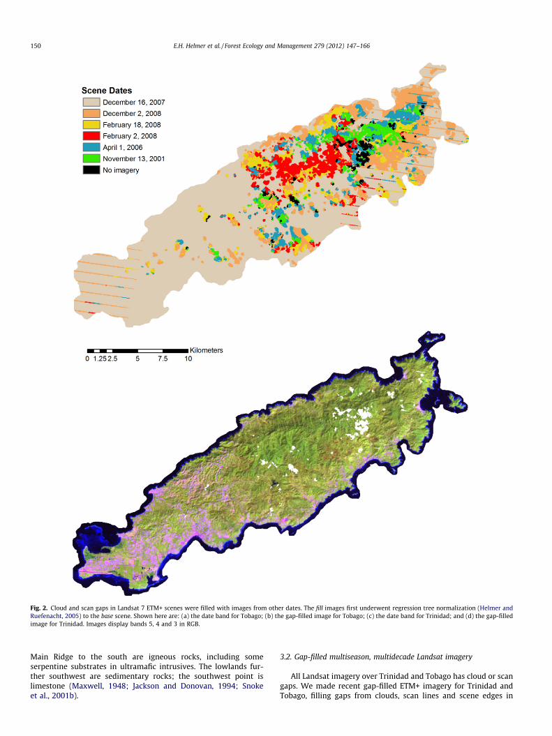
Fig. 2. Cloud and scan gaps in Landsat 7 ETM+ scenes were filled with images from other dates. The fill images first underwent regression tree normalization (Helmer andRuefenacht, 2005) to the base scene. Shown here are: (a) the date band for Tobago; (b) the gap-filled image for Tobago; (c) the date band for Trinidad; and (d) the gap-filledimage for Trinidad. Images display bands 5, 4 and 3 in RGB.


Main Ridge to the south are igneous rocks, including someserpentine substrates in ultramafic intrusives. The lowlands fur-ther southwest are sedimentary rocks; the southwest point islimestone (Maxwell, 1948; Jackson and Donovan, 1994; Snokeet al., 2001b).

3.2. Gap-filled multiseason, multidecade Landsat imagery

All Landsat imagery over Trinidad and Tobago has cloud or scangaps. We made recent gap-filled ETM+ imagery for Trinidad andTobago, filling gaps from clouds, scan lines and scene edges in

Fig. 2 (continued)


reference scenes from the early dry season of 2007 (December)with image data from fill scenes (Table 3 and Fig. 2). In our priorwork mapping physiognomic forest types, image gaps came only

from clouds, as we used imagery dated before late May of 2003.Here scan gaps added uncertainty to our ability to map forestassociations. Each fill scene first underwent regression-tree


normalization to the 2007 data. This nonlinear normalization min-imizes the atmospheric, phenological and sensor differences be-tween the base and fill scenes and is described elsewhere(Helmer and Ruefenacht, 2005, 2007).

In Trinidad, we mapped land cover with the 2007 gap-filledimagery. We then mapped forest association with separate classi-fication models that were applied only to forests. For these classi-fication models of forest association, we added gap-filled imageryfrom the late dry season (see below). Tobago has far fewer matureforest associations than Trinidad; there we simultaneouslymapped land cover and forest associations with the 2007 gap-filledimagery.

We used the early dry season imagery for land-cover mappingbecause forest is most distinct from nonforest then: deciduous for-ests are still leafed out, making them more spectrally distinct fromnonforest. In contrast in the late dry season, leaf loss for deciduoustropical tree species peaks, causing confusion between deciduousforest and nonforest. In the wet season, flooding helps distinguishforested wetlands, but dense herbaceous cover is greened up andmay be spectrally similar to young forest.

In the course of this work we observed that imagery from thelate dry season (late March–early May) might be helpful for distin-guishing among the many seasonal forest associations in Trinidad,most of which would simply be classified as moist forests in the lifezone system. Consequently, for mapping forest type we made threegap-filled images from the mid- to late dry season for mapping for-est type with three Landsat TM scenes from the years 1985–1987(Table 3). Because each of these 1980s images displayed slightlydifferent phenology, we sought gap-filled images that representedthe unique phenology of each scene, and so each scene served as abase scene to which we then normalized the other two scenes.Whether this form of synthetic multiseason imagery would im-prove results had not been tested for mapping tropical forestassociations.

Another reason for using imagery from the 1980s is that addingimage bands from previous decades to the set of spectral bandsbeing classified helps distinguish mature and old-growth tropicalforest from secondary forest (Kimes et al., 1999; Helmer et al.,2000). Being �20 years old, the 1980s data might help distinguishforest younger than �15–20 years old in the 1980s (up to �35–40 years old in 2007) from older (‘‘mature’’) forests (assuming thatforest regrowth becomes indistinct from mature forest after about15–20 years).

3.3. Cloud masking

In making the mosaics, we masked clouds and cloud shadowswith: (1) an algorithm that identified clouds and potential cloudshadows with a series of models in ERDAS Imagine and a short rou-tine in Interactive Data Language (IDL); (2) an IDL program thatidentified actual cloud shadow from clouds, potential cloud sha-dow and solar geometry which was partly based on Choi andBindschadler (2004); and (3) manual refinement. The algorithm re-quires some clear area over land and water, and clouds must be nowarmer than water. It ignores snow and ice.

The algorithm to identify clouds and potential cloud shadowsuses Histogram Fitting for Mapping (HFM), which Helmer et al.(2009) describe for making a forest mask with image-specificthresholds found from image histograms. Water and land pixelsare identified with the Shuttle Radar Topography Mission (SRTM)Water Body Dataset (SWBD) (NGA, 2003). Next, IDL fits a normaldistribution to the histogram of the thermal infrared band (TIR-band6) for water pixels, and then for land pixels. Cool and warmclouds are found as pixels cooler than or as cool as most water pix-els, respectively, or cooler than land if land is cooler than water.Clouds are preliminarily masked from the image, and the parame-

ters are again estimated for each band by fitting a normal distribu-tion to the new histograms of water and land. Pixels are thenmasked from the identified clouds if they are darker than or as darkas most water in the second shortwave-infrared band (SWIRband7),removing warm or shallow water. Cool land is then removed fromthe cloud mask by removing pixels that are as dark as most land inthe blue band. Potential cloud shadow over land is mapped asareas that are darker in bands 4 and 5 than most land.

Next, each cloud patch is gradually shifted in the direction ofthe shadows. The distance of maximum overlap between pixelsin the shifting cloud patch and pixels of potential cloud shadowis found as the peak of the distribution of overlapping pixels for dif-ferent distances. The shifted cloud patch is expanded slightly andtaken as identified cloud shadow. For Landsat ETM+ imagery withscan-line gaps, a majority filter fills scan gaps with clouds or poten-tial cloud shadows where these elements are in the image data sur-rounding gaps. Final manual refinement was followed by adding athree-pixel buffer to both the clouds and the identified cloud shad-ows. The buffer removes mixed pixels that occur around cloudedges.

3.4. Collecting reference data on tropical forest association

We used the hierarchical classification system of Beard (1944a,1946a) who classified native forests in Trinidad and Tobago andmapped their distributions on public lands (which comprise about40% of the land). The system starts with floristic groups that are‘‘recognizable by diagnostic species.’’ The associations are groupedinto alliances of canopy dominants and then into formations basedon physiognomic factors, primarily structure, deciduousness, andother characteristics of leaf type (Tables 1 and 2; local names inS1–S2). Formations ‘‘express a habitat determined by the interplayof the environmental factors of climate, topography, and soil’’(Beard, 1944b, 1946a). Montane seasonal forests, for example,are ‘‘seasonal’’ because of the importance of deciduous species,which are more common in this forest than in other montane for-est because it occurs on more freely draining limestone substrates.The associations within a formation, though floristically defined,usually also differ slightly in physiognomy. The semi-evergreenassociations differ in deciduousness, for example, as do some ofthe seasonal evergreen associations. Vegetation physiognomy af-fects spectral response in satellite imagery, particularly deciduous-ness and canopy development. It follows that because severalfloristic associations are physiognomically distinct, they may alsobe distinct in multispectral imagery if it is dated from the correctseason or year.

Beard based his system on strip surveys conducted from 1927–1933 and 1941–1942, and aerial photos from 1938 (scale1:40,000). All trees >9.9 cm diameter at breast height (dbh) werecounted along continuous, 10-m wide transects, and then summedby species over each 200-m long section. The plot networks weredense: transects in central and southern Trinidad, for example,were spaced only 2 km apart, resulting in about 1600 plots.

Given the high spatial density and large number of plots Beardused, and the detailed descriptions and tallies of the species com-position and deciduousness of associations, we assumed that thisclassification system is valid for forests where large-scale clearingfor agriculture did not occur since the surveys, even though it wasnot based on modern ordination techniques. We also assumed thatwe could rely on the Beard maps as one information source whenlearning to identify forest classes in fine resolution imagery. Ourconclusions are conditioned on these assumptions. Forest associa-tions on public lands were again mapped with aerial photos from1969 and field work conducted in 1979–1980 (FRIM, 1992), andthe mapping results are almost identical. We modified the names

Table 1Forest classes mapped for Trinidad; mature forest classes are those from Beard (1946a,b).a

Forest Formation and Association according to Beard (1946a,b) Symbol Identifying sourcesa

Dry evergreen forest–littoral woodland (canopy)Coccoloba uvifera–Hippomane mancinellab LWS 1 m Img, Maps, Fieldb

Roystonea oleracea–Manilkara bidentatab LWP 1 m Img, Mapsb

Deciduous seasonal forest (canopy)Machaerium robinifolium–Lonchocarpus punctatus–Bursera simaruba Ss 1 m Img, Field, L7 200303

Deciduous to semi-evergreen seasonal forest (canopy)Protium guianense–Tabebuia serratifolia ecotone and Peltogyne floribunda–T. serratifolia–P. guianense Ip 1 m Img, Field, L7 200303

Semi-evergreen seasonal forest (canopy)P. floribunda–Mouriri marshallii Pbl Plots, 1 m Img, Maps, FieldTrichilia pleeana–Brosimum alicastrum–Bravaisia integerrima Aj Plots, 1 m Img, Maps, FieldT. pleeana–B. alicastrum–Protium insigne Ag Plots, 1 m Img, Maps, FieldB. alicastrum–Ficus yoponensisb Af Maps, L5 1987b

Evergreen seasonal forest (emergents/canopy/subcanopy)Aniba panurensis and A. trinitatis-Carapa guianensis/Ligania biglandulosa Cd Maps, FieldA. panurensis and A. trinitatis – Carapa guianensis – Eschweilera subglandulosa/Pentaclethra macroloba/Attalea maripa Cco Plots, 1 m Img, Maps, Field,

L7200301C. guianensis–Pachira insignis – E. subglandulosa/P. macroloba/Sabal sp. Cca Plots, 1 m Img, Maps, FieldE. subglandulosa–P. insignis–C. guianensis/Clathrotropis brachypetala/A. maripa Cb Plots, 1 m Img, Maps, Field,Mora excelsa–C. guianensis/P. macrolobac Cm Plots, 1 m Img, Maps, Field

Montane rain forest (Canopy)Transitional seasonal evergreen to lower montane Cd-LMF 1 m Img, MapsByrsonima spicata–Licania ternatensis–Sterculie pruriens (Lower) LMF Maps, FieldInga macrophylla–Guarea guara (seasonal)b SMF Maps, L5 1987b

Transitional Lower Montane – Montane LMF-MF 1 m Img, MapsRicheria grandis–Eschweilera trinitensis (Montane Cloud) MF 1 m Img, Maps, Field

Forested WetlandsMangrove (includes different associations)d ESM 1 m Img, Maps, FieldOther swamp communitiese ESO 1 m Img, Maps, Field

Young secondary forest classesHevea brasiliensis – former plantation Br 1 m Img, Field, L7200301Young secondary forest (<15–20 yr) YSF 1 m Img, FieldYoung secondary forest (<35–40 yr) or abandoned or semi-active woody agriculture YSF-

Wag1 m Img, Field

Young secondary forest – former Cocos nucifera plantation YSF-C 1 m Img, FieldBambusa vulgaris YSF-B 1 m Img, Field

Tree plantationsTectona grandisb PT 1 m Img, Fieldb

Pinus caribaeab PP 1 m Img, Fieldb

Otherb PO 1 m Img, Fieldb

a The latin names for seasonal and semi-evergreen forest types are altered to better represent canopy dominance. 1Plots = Plots; Field = field identification; 1 m Img = 61-mimagery; Maps = Maps from air photos and plots (Beard (1946a,b); FRIM, 1992); L7 = Landsat 7 ETM+; L7 2003 03 = L7 from 03/31/2003; L7 2003 01 = L7 from 01/19/2003; L51987 = Landsat 5 TM dated 05/07/1987.

b Manually delineated.c Both modeled and manually delineated.d Associations may include these species: Rhizohpora mangle, R. harrisonii, R. racemosa, Avicennia germinans, A. Schaueriana, Laguncularia racemosa, or Conocarpus erectus.e The Class other swamp communities was manually differentiated, based on 61-m imagery, into palm swamp (Roystonea oleracea or Mauritia flexuosa), swamp forest

(Pterocarpus officinalis); swamp forest ecotone (Carapa guianensis–Ptercarpus officinalis), marsh forest (Manicaria saccifera–Jessenia oligocarpa–Euterpe precatoria), or marshforest – seasonal evergreen ecotone.


of evergreen seasonal associations, adding other diagnostic domi-nant species that Beard mentions in addition to the timber species.

Data for training and testing the classification models camefrom assigning land cover or forest type to patches of about 16or fewer pixels (but only one to four pixels for low-density urbanlands). The data sources were: (1) three weeks of field work inwhich experts identified forest association in locations throughoutthe islands; (2) the locations of 241 inventory plots that expertshad labeled to forest association; and 3) learning to identify manyof the forest associations in fine resolution imagery (or in two casesin Landsat imagery), based on the field work, plots, and unique his-torical work by Beard (1944a, 1946a). The large number of Beard’sassociations that we could identify was unexpected, and we givemore details in the results section.

Fine resolution imagery (61 m) was available for the entirestudy area and dated from October 2000 to August 2009. Most datawas from 2004 to 2007. It included island-wide tiled mosaics of

pan-sharpened, true color IKONOS images (examples shown inS3); island-wide tiled mosaics of black-and-white, orthorectifieddigital air photos; and pan-sharpened, true color images from Dig-ital Globe that were viewable with Google Earth. The Google Earthimages included most of the IKONOS images above, but also in-cluded more than one date of fine resolution imagery for mostplaces.

Two or more distinct spectral classes were discernible for someforest types. We separated such classes in decision-tree modelsand then recombined them in the final map and accuracy assess-ment. For example, a gradient of decreasing greenness from westto east was evident for two of the lowland seasonal evergreen asso-ciations. This gradient likely reflects the gradient of increasingdeciduousness that Beard (1946a) mentions. As in prior work, asunlit and shadowed spectral class represented each forest typein hilly areas. We also separated the training pixels for Mora forestsinto three geographic regions: south, central and Northern Range.

Table 2Forest classes mapped for Tobago; mature forest classes are those from Beard (1944a,b).

Forest formation and association Code Identifying sourcesa

Dry evergreen forest – littoral woodlandCoccoloba uvifera–Hippomane mancinellab Manilkara bidentatab LWSb XFBab 1 m Img, Maps, Field 1 m Img, L72000 08

Deciduous seasonal forestBursera simaruba–Coccothrinax barbadensis Ssd 1 m Img, Maps, Field

Semi-evergreen seasonal forestHura crepitans–Tabebuia chrysantha–Spondias mombin Sch 1 m Img, Maps, Field

Lowland rain forestCarapa guianensis–Euterpe precatoria Ccp 1 m Img, Maps, Field

Xerophytic rain forestManilkara bidentata–Guettarda scabra XFBb 1 m Img, Maps, L72000 08

Lower montane rain forestLicania biglandulosa – Byrsonima spicata LMF 1 m Img, Maps, Field

Young secondary forest classesYoung secondary forest (<15-20 yr), abandoned woody agriculture YSF-Wag 1 m Img, FieldSecondary forest – former Cocus nucifera plantationb YSF-Cb 1 m Img, FieldBambusa vulgaris YSF-B 1 m Img, Field

Forested wetlandsMangrove ESM 1 m Img, Maps, FieldOther wooded wetlands ESO 1 m Img, Maps, Field

a Field = field identification; 1 m Img = 61-m imagery; Maps = maps from air photos and plot data (Beard (1944a,b)) and maps, air photos and fieldwork from FRIM (1992);L72000 = Landsat 7 ETM+, 001/052, dated 08/06/2000.

b Manually delineated.

Table 3Four gap-filled Landsat image mosaics were created for Trinidad and one for Tobago from the 19 scenes listed here. Each mosaic included a reference, or base scene. The clear partsfrom other scene dates, or fill scenes, then filled the cloudy parts of the base scene after undergoing normalization to the base scene with the regression tree method of Helmerand Ruefenacht (2005). Fill scenes are listed in the order that they filled cloudy areas in the base scene (i.e., top to bottom). Scene types: L5 = Landsat 5 TM; L7 = Landsat 7Enhanced TM.

Dates and types of scenes in gap-filledmosaics (month/day/year)

Percent of studyarea Dates and types of scenes in gap-filledmosaics (month/day/year)

Percent of study area

Trinidad 2007, path/row 233/053 Trinidad 1980s, path/row 233/05312/16/2007 – L7 57 03/14/1985 – L5 4603/05/2002 – L7 21 05/04/1986 – L5 2201/29/2001 – L7 13 05/07/1987 – L5 1004/17/2006 – L7 3.301/30/2007 – L7 1.5 05/04/1986 – L5 4203/21/2008 – L7 0.7 03/14/1985 – L5 2702/03/2006 – L7, 001/053 1.3 05/07/1987 – L5 1002/11/2003 – L7, 001/053 1.401/24/2008 – L7 0.02 05/07/1987 – L5 3410/25/2000 – L7 0.3 03/14/1985 – L5 29

05/04/1986 – L5 14

Tobago 2007, path/row 233/05212/16/2007 – L7 6312/02/2008 – L7 1402/18/2008 – L7 5.702/02/2008 – L7 6.004/01/2006 – L7 6.211/13/2001 – L7 3.9


3.5. Classifications and classification comparisons

To create classification mapping models, we applied the deci-sion-tree software See5 to text files that list class assignment andvalues for spectral and ancillary predictor layers for each referencepixel. To produce each map, we applied the models from See5 tothe stack of spectral and ancillary data layers with software fromRuefenacht et al. (2008).

A randomly-selected 90% of the reference data served to traineach classification model, leaving 10% of the data for estimatingmodel error. On average, then, about one to two pixels per patchwere available for testing. Calculating classification accuracy frompixels that are randomly selected from multi-pixel patches oftraining data likely yields optimistic error estimates. The bias

arises because pixels within a patch are likely to be more similarto each other than to other pixels of the same class. Limiting testdata to 10% of the reference data reduces this bias from the morecommonly withheld proportion of 30%, but probably does not re-move it. Sufficient resources were not available for a completelyindependent accuracy assessment (Sesnie et al., 2008).

We used one decision-tree classification model to simulta-neously map both land cover and forest type for Tobago, as Tobagohas only seven main forest associations that are closely related totopography. The model used the gap-filled image centered on2007 and the other predictor layers listed in the next section.

Trinidad was divided into two mapping zones: the NorthernRange was one; the rest of Trinidad (the ‘‘lowlands’’) was the other.With the decision-tree software described above, we first mapped


land cover for the two Trinidad zones with the gap-filled imagecentered on 2007. We then mapped forest type for the two Trini-dad zones for the areas that the land-cover models classified as for-est, using the gap-filled imagery centered on 2007, all three of thegap-filled images from the 1980s, and the other predictor layersdescribed below. In those results Mora forests in the southeastand Northern Range showed more confusion with other foresttypes. Consequently, we manually cleaned up the result for Moraforests in those areas and then overlaid the edited Mora forestsonto forest types as mapped after excluding Mora training pointsin those areas.

To test if the gap-filled imagery from the 1980s and the thermalband improved classifications, we compared overall accuracy,class-specific accuracies, and the Kappa coefficient of agreementof models that used various band combinations. We testedwhether overall and class-specific accuracies differed significantlyvia the McNemar test for comparing related proportions (Foody,2009). Comparisons were of (1) land cover with vs. without thegap-filled thermal band; and (2) for Trinidad, forest associationwith vs. without one or more of the gap-filled images from the1980s.

3.6. Ancillary environmental predictor layers

We considered the following predictor layers for the decision-tree classification models: spectral bands and indices from thegap-filled imagery; maps of rainfall and temperature (Hijmanset al., 2005); and topography (Farr et al., 2007), geology (Suter,1960; Snoke et al., 2001b) and geographic position. Hijmans et al.(2005) mapped climate at 1-km resolution based on climate sta-tion data and topography. Their data did not include the densernetwork of rain gauges set up by the local water authority, butthose rainfall data were not available to us. Topographic layers in-cluded elevation, slope, slope position, curvature, sine and cosineof aspect, topographic shading for the time of the base scene for

Fig. 3. Forest association and land cover for Tobago were mapped with decision-tree clasassociations are classified according to the system of Beard (1944).

each gap-filled image, and topographic relative moisture index(TRMIM) (Manis et al., 2002). We used these topographic deriva-tives to represent soil drainage.

Spectral data included all bands from each Landsat mosaic, adate band (e.g. Fig. 2a and c) and six spectral indices. The indiceswere tasseled cap (TC) brightness, greenness and wetness (Cristand Cicone, 1984; Huang et al., 2002), the wetness–brightness dif-ference index (WBDI) (Helmer et al., 2009), the normalized differ-ence vegetation index (NDVI), and the normalized differencestructure index (NDSI) (Hardisky et al., 1983; Helmer et al., 2010):

WBDI ¼ TC Wetness� TC Brightness ð1ÞNDVI ¼ ðNIRb4 � REDb3Þ=ðNIRb4 þ REDb3Þ ð2ÞNDSI ¼ ðNIRb4 � SWIRb5Þ=ðNIRb4 þ SWIRb5Þ ð3Þ

3.7. Manual delineation and editing

Several forest associations were manually delineated (Tables 1and 2). We manually delineated managed and former timber plan-tations, including teak, Caribbean pine and abandoned Brazilianrubber. Though usually spectrally distinct from adjacent forest,delineating them was fast, thanks to their regular boundaries andlimited number, and would reduce confusion among other classes.Spanish cedar plantations are also common in Trinidad. Though welocated many patches of it during field work, most of them weretoo small to be clearly identifiable in the Landsat imagery. We alsomanually delineated the two littoral forest associations. Many ofthe patches were narrow, resulting in pixels being mixed withwater, sand or wetland, making their spectral signatures highlyvariable. Nonforested wetlands were also manually delineateddue to large signature variability. Nonmangrove forested wetlandswere one class in decision-tree models and then manually dividedinto subclasses. Most other manual editing corrected confusion be-tween Mora forests and other seasonal evergreen associations, or

sification of gap-filled Landsat 7 imagery centered on December 2007. Mature forest

Fig. 4. Before mapping forest association, land cover was mapped for Trinidad with decision-tree classification of gap-filled Landsat 7 imagery centered on December 2007,which is the early dry season. Forest association was then mapped for those areas classified as forest with the gap-filled imagery from 2007 plus three gap-filled images fromthe 1980s that were from the mid to late dry season. Mature forest associations are classified according to the system of Beard (1946a).


corrected scattered pixels of agriculture that were misclassified asurban lands.

4. Results

The final map of land cover and forest associations for Tobago(Fig. 3) included the most accurate overall classification, which in-

cluded the thermal band. The final map for Trinidad (Fig. 4) com-bined the most accurate land-cover classification, which includedthe thermal band, the most accurate classifications of forest asso-ciation, which included all of the gap-filled images from the1980s, and the edited Mora forests (Fig. 5). Where residual gaps ex-isted in the 1980s gap-filled imagery, forest association wasmapped with only the 2007 gap-filled image.

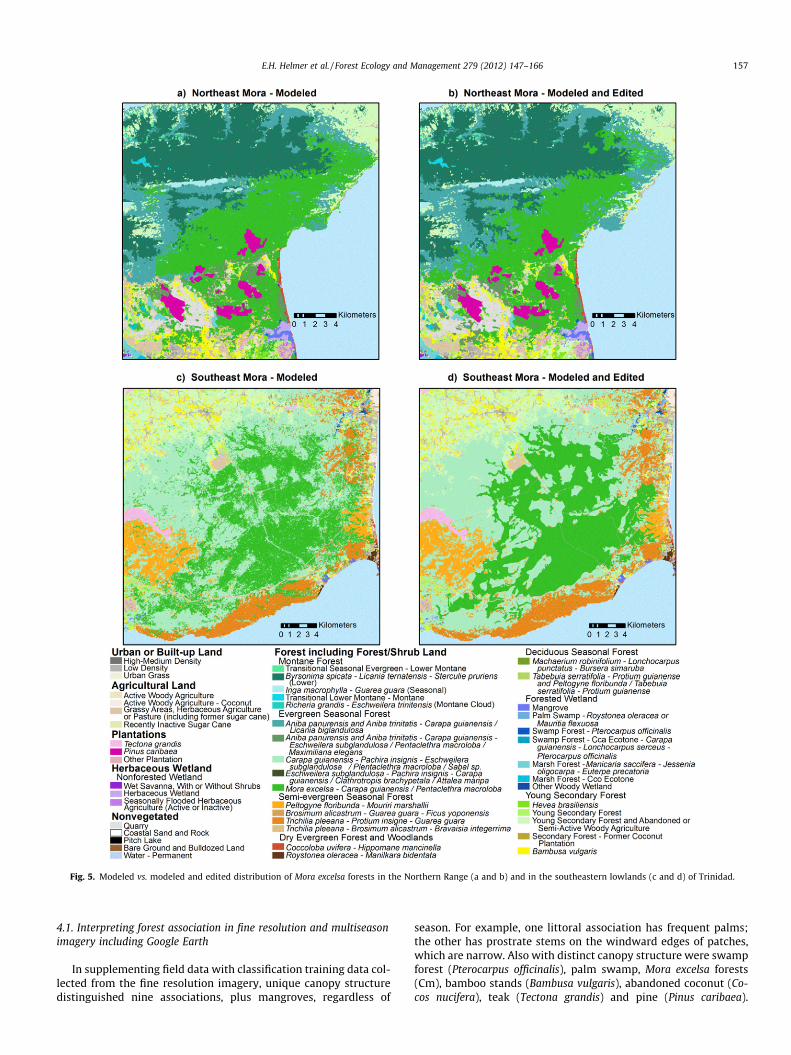
Fig. 5. Modeled vs. modeled and edited distribution of Mora excelsa forests in the Northern Range (a and b) and in the southeastern lowlands (c and d) of Trinidad.


4.1. Interpreting forest association in fine resolution and multiseasonimagery including Google Earth

In supplementing field data with classification training data col-lected from the fine resolution imagery, unique canopy structuredistinguished nine associations, plus mangroves, regardless of

season. For example, one littoral association has frequent palms;the other has prostrate stems on the windward edges of patches,which are narrow. Also with distinct canopy structure were swampforest (Pterocarpus officinalis), palm swamp, Mora excelsa forests(Cm), bamboo stands (Bambusa vulgaris), abandoned coconut (Co-cos nucifera), teak (Tectona grandis) and pine (Pinus caribaea).


Apparent differences in water level also helped distinguish for-ested wetlands from other forests. Mora excelsa forests, which area monodominant type, have a smoother canopy that is 15 m tallerand has larger crowns than adjacent types (S3-a). Beard could dis-tinguish this association in air photos.

For an additional seven associations, plus abandoned woodyagriculture, we identified unique canopy features that were onlypresent in certain seasons or dates of the fine resolution imagery.Two or more fine resolution images were available for nearly allof the study area. Images displaying the seasonal image elements

Table 4Overall and class-specific overall accuracy for Tobago classification of land cover and fore

Forest formation and association Code

Kappa coefficient of agreementOverall accuracy (%)

Dry evergreen forest – littoral woodlandCoccoloba uvifera–Hippomane mancinella LWS

Deciduous seasonal forestBursera simaruba–Coccothrinax barbadensis Ssd

Semi-evergreen seasonal forestHura crepitans–Tabebuia chrysantha–Spondias mombin Sch

Xerophytic rain forestManilkara bidentata–Guettarda scabra XFBb

Lowland rain forestCarapa guianensis–Euterpe precatoria Ccp

Lower montane rain forestLicania biglandulosa–Byrsonima spicata LMF

Young secondary forest classesYoung secondary forest (<15-20 yr) YSF-WagBambusa vulgaris YSF-B

Edaphic swamp communitiesMangrove ESMOther wooded wetlands ESO

Nonforest classesHerbaceous agricultureWaterUrban, high densityUrban, low densityGrassy areas, pasture

Fig. 6. For the Tobago classification model, the percentage of cases in w

that identified association were available for at least half of the ex-tent of the seven associations. Examples of these elements are thelowland seasonal evergreen association Cco, which has a canopypunctuated by dark crowns in scenes from late April (S3-b), prob-ably the result of flushing leaves which can be red to brown in col-or, distinguishing it from another lowland seasonal evergreen type(Cca). The same dark crowns distinguished the two seasonal ever-green associations of the Northern Range (Cd and transitional Cd)from types at higher elevations. Differences in relative deciduous-ness showed distinct boundaries between three lowland semi-

st type. The relative differences in bold typeface are significant at p < 0.05.

Excluding thermal Including thermal Relative difference (%)

0.93 ± 0.01 0.93 ± 0.0194 94 0

64 72 13

98 98 0

90 91 1

91 93 2

94 92 �2

96 96 0

89 89 079 79 0

96 96 086 86 0

73 93 27100 100 094 94 091 88 �397 96 �1

hich the indicated layer was used in at least one classification rule.


evergreen associations (Pbl, Aj and Ag). Based on deciduousness wecould also distinguish seasonal from semi-evergreen associations,including in an area that Beard maps a mixture of the two (Ccavs. Ag). The semi-evergreen association is either more deciduousor a brighter green (caused by leaf flush of deciduous species) thanthe seasonal evergreen one (Fig. S3-c). Abandoned woody agricul-ture was also distinct in fine resolution imagery if Erithryna poepp-igiana was in bloom. It is a nitrogen-fixing legume withconspicuous coral-colored flowers that farmers plant to shadeand fertilize coffee or cocoa (Fig. S3-d). This feature was mainlypresent in the Northern Range.

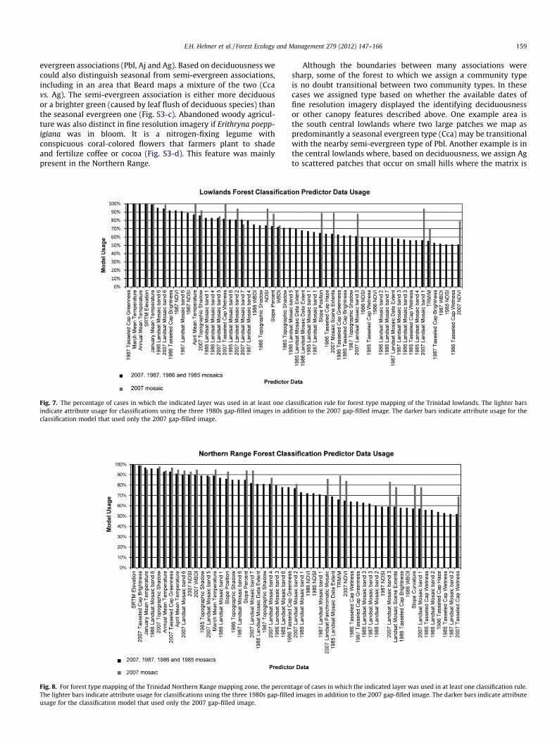
Fig. 7. The percentage of cases in which the indicated layer was used in at least one clindicate attribute usage for classifications using the three 1980s gap-filled images in addclassification model that used only the 2007 gap-filled image.

Fig. 8. For forest type mapping of the Trinidad Northern Range mapping zone, the percenThe lighter bars indicate attribute usage for classifications using the three 1980s gap-filleusage for the classification model that used only the 2007 gap-filled image.

Although the boundaries between many associations weresharp, some of the forest to which we assign a community typeis no doubt transitional between two community types. In thesecases we assigned type based on whether the available dates offine resolution imagery displayed the identifying deciduousnessor other canopy features described above. One example area isthe south central lowlands where two large patches we map aspredominantly a seasonal evergreen type (Cca) may be transitionalwith the nearby semi-evergreen type of Pbl. Another example is inthe central lowlands where, based on deciduousness, we assign Agto scattered patches that occur on small hills where the matrix is

assification rule for forest type mapping of the Trinidad lowlands. The lighter barsition to the 2007 gap-filled image. The darker bars indicate attribute usage for the

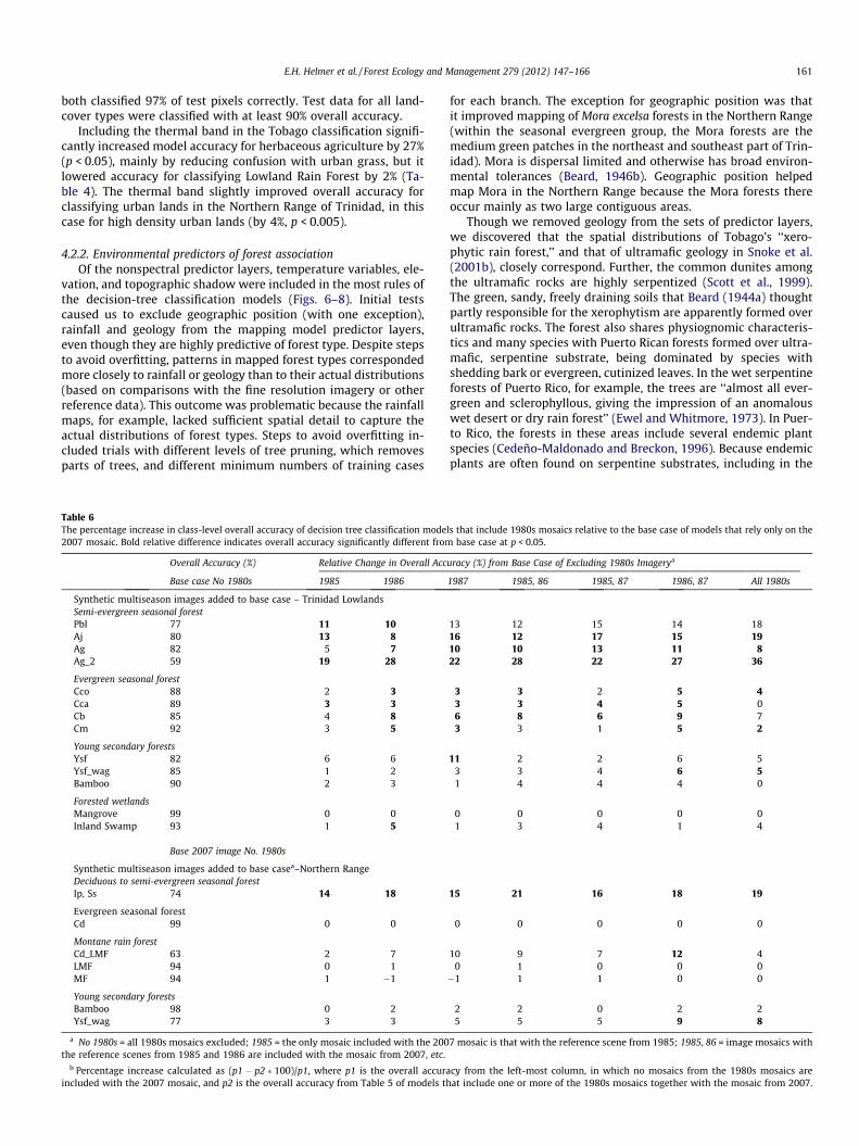
tage of cases in which the indicated layer was used in at least one classification rule.d images in addition to the 2007 gap-filled image. The darker bars indicate attribute

Table 5A comparison of overall accuracies for Trinidad, including class-level accuracies. Decision tree classification models that include the gap-filled image from 2007, but that excludeone to three of the 1980s gap-filled images, are compared against models that include all of the gap-filled images (N = 8525 for Trinidad’s lowlands and 8757 for the rest ofTrinidad). In the Lowlands, the most accurate models used at least two of the gap-filled images from the 1980s, particularly those representing the driest conditions.

Overall accuracy (%) and significance of difference from base case of including all 1980s imageryc

No. 1980s 1985 1986 1987 1985, 86 1985, 87 1986, 87 Base case All 1980s

Synthetic multiseason images included with 2007 image a – Trinidad lowlandsKappa statisticb 0.84 0.88 0.89 0.90 0.90 0.90 0.91 0.92Overall 86*** 90*** 91*** 91*** 91*** 92** 93 93

Semi-evergreen seasonal forestPbl 77*** 87* 86** 89 88* 91 90 91Aj 80*** 92 87*** 95 91* 96 93* 96Ag 82*** 86*** 88* 91 91 95 92 93Ag_2 59*** 73*** 82 76* 82 77* 82 83

Evergreen seasonal forestCco 88** 89* 91 91 91 90* 92 93Cca 89*** 92** 92** 92** 92** 93* 93 94Cb 85** 89* 93 91 93 91 94 93Cm 92 94 97 95 95 93 97 95

Young secondary forestsYSF 82 88 88 92 84 84 88 87YSF-Woody Ag 85* 86 87 88 88 89 91 89YSF-Bamboo 90 92 93 91 94 94 94 93

Forested wetlandsMangrove 99 100 100 99 100 100 99 99Inland Swamp 93 95 98 95 96 97 95 97

Synthetic multiseason images included with 2007 Imagea – Trinidad Northern RangeKappa statisticb 0.89 0.90 0.91 0.91 0.91 0.91 0.91 0.91Overall 93** 94 94 94 94 94 94 94

Deciduous to semi-evergreen seasonal forestIp, Ss 74** 86 90 87 93 88 90 88

Evergreen seasonal forestCd 99 99 99 99 99 99 99 99

Montane rain forestCd_LMF 63 64 68 70 69 68 71 65LMF 94 95 95 95 95 94 95 95MF 94 95 93 93 95 95 94 94

Young secondary forestsYSF-Woody Ag 77* 79 79 80 80 81 84 83YSF-Bamboo 98 98 100 100 100 98 100 100

a No 1980s = all 1980s mosaics excluded; 1985 = the only mosaic included with the 2007 mosaic is that with the reference scene from 1985; 1985, 86 = image mosaics withthe reference scenes from 1985 and 1986 are included with the mosaic from 2007, etc.

b The 95% confidence interval for all Kappa estimates rounds to ±0.01; differences between Kappa estimates that are larger than ±0.01 are significant at p < 0.05.c McNemar test for related proportions.* p < 0.05.

** p < 0.005.*** p < 0.0005.


Cca. These patches likely receive more rainfall than the Ag patchescloser to the coast. They are likely transitional between the Ag andCca communities.

An additional four associations have distinct boundaries in par-ticular Landsat image dates (Tables 1 and 2), two of which we man-ually digitized from specific scenes (SMF and Br). Tobago’sxerophytic rain forest (XfBb) displayed a larger band 4:5 ratio inwet-season imagery, which we have observed occurs in otherCaribbean forest types with hard leaves and a wind-clipped can-opy, though we have not seen this observation mentioned else-where. Other examples were distinct in a specific image date(Table 1) because of a leaf-off condition, including the distinctionbetween deciduous and semi-evergreen forests on the Chaguara-mas Peninsula in northwest Trinidad (Ss vs. Ip); former plantationsof Brazilian rubber (Hevea brasiliensis); and the main areas of themontane seasonal forest (SMF). In these images these forest asso-ciations reflected more light in the red band and less in the nearinfrared band as compared with adjacent forest. The image fromthe 1987 drought was the only image we found in which montaneseasonal forests, which are more seasonal because they occur on

more freely draining limestone substrates, had dropped so muchfoliage as to be distinct from surrounding forest. Another note isthat strategic display of Landsat bands 7, 2 and the wetness–brightness difference index (WBDI) revealed the extent of lowlandMora. In this display it appears greener on flat lands than otherold-growth forest because it tends to be brighter in the visibleband 2, possibly because its monodominant and therefore smooth-er canopy has less shadow.

4.2. Classification models

4.2.1. Land-cover classifications and the influence of the thermal bandIn Tobago (Fig. 3), the test data for land cover and forest associ-

ation were classified with an overall accuracy of 94% (Table 4).Class-specific accuracies for test data on forest associations rangedfrom 72% to 98% (Table 4). Though we did not make multiseasonimage mosaics for Tobago, it has fewer associations, most of whichare closely related to topography. The land-cover classificationmodels for the Northern Range and lowlands of Trinidad (Fig. 4)


both classified 97% of test pixels correctly. Test data for all land-cover types were classified with at least 90% overall accuracy.

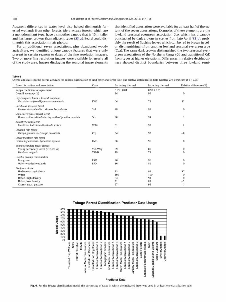
Including the thermal band in the Tobago classification signifi-cantly increased model accuracy for herbaceous agriculture by 27%(p < 0.05), mainly by reducing confusion with urban grass, but itlowered accuracy for classifying Lowland Rain Forest by 2% (Ta-ble 4). The thermal band slightly improved overall accuracy forclassifying urban lands in the Northern Range of Trinidad, in thiscase for high density urban lands (by 4%, p < 0.005).

4.2.2. Environmental predictors of forest associationOf the nonspectral predictor layers, temperature variables, ele-

vation, and topographic shadow were included in the most rules ofthe decision-tree classification models (Figs. 6–8). Initial testscaused us to exclude geographic position (with one exception),rainfall and geology from the mapping model predictor layers,even though they are highly predictive of forest type. Despite stepsto avoid overfitting, patterns in mapped forest types correspondedmore closely to rainfall or geology than to their actual distributions(based on comparisons with the fine resolution imagery or otherreference data). This outcome was problematic because the rainfallmaps, for example, lacked sufficient spatial detail to capture theactual distributions of forest types. Steps to avoid overfitting in-cluded trials with different levels of tree pruning, which removesparts of trees, and different minimum numbers of training cases

Table 6The percentage increase in class-level overall accuracy of decision tree classification mode2007 mosaic. Bold relative difference indicates overall accuracy significantly different from

Overall Accuracy (%) Relative Change in Overall Acc

Base case No 1980s 1985 1986

Synthetic multiseason images added to base case – Trinidad LowlandsSemi-evergreen seasonal forestPbl 77 11 10Aj 80 13 8Ag 82 5 7Ag_2 59 19 28

Evergreen seasonal forestCco 88 2 3Cca 89 3 3Cb 85 4 8Cm 92 3 5

Young secondary forestsYsf 82 6 6Ysf_wag 85 1 2Bamboo 90 2 3

Forested wetlandsMangrove 99 0 0Inland Swamp 93 1 5

Base 2007 image No. 1980s

Synthetic multiseason images added to base casea–Northern RangeDeciduous to semi-evergreen seasonal forestIp, Ss 74 14 18

Evergreen seasonal forestCd 99 0 0

Montane rain forestCd_LMF 63 2 7LMF 94 0 1MF 94 1 �1

Young secondary forestsBamboo 98 0 2Ysf_wag 77 3 3

a No 1980s = all 1980s mosaics excluded; 1985 = the only mosaic included with the 200the reference scenes from 1985 and 1986 are included with the mosaic from 2007, etc.

b Percentage increase calculated as (p1 � p2 � 100)/p1, where p1 is the overall accuraincluded with the 2007 mosaic, and p2 is the overall accuracy from Table 5 of models th

for each branch. The exception for geographic position was thatit improved mapping of Mora excelsa forests in the Northern Range(within the seasonal evergreen group, the Mora forests are themedium green patches in the northeast and southeast part of Trin-idad). Mora is dispersal limited and otherwise has broad environ-mental tolerances (Beard, 1946b). Geographic position helpedmap Mora in the Northern Range because the Mora forests thereoccur mainly as two large contiguous areas.

Though we removed geology from the sets of predictor layers,we discovered that the spatial distributions of Tobago’s ‘‘xero-phytic rain forest,’’ and that of ultramafic geology in Snoke et al.(2001b), closely correspond. Further, the common dunites amongthe ultramafic rocks are highly serpentized (Scott et al., 1999).The green, sandy, freely draining soils that Beard (1944a) thoughtpartly responsible for the xerophytism are apparently formed overultramafic rocks. The forest also shares physiognomic characteris-tics and many species with Puerto Rican forests formed over ultra-mafic, serpentine substrate, being dominated by species withshedding bark or evergreen, cutinized leaves. In the wet serpentineforests of Puerto Rico, for example, the trees are ‘‘almost all ever-green and sclerophyllous, giving the impression of an anomalouswet desert or dry rain forest’’ (Ewel and Whitmore, 1973). In Puer-to Rico, the forests in these areas include several endemic plantspecies (Cedeño-Maldonado and Breckon, 1996). Because endemicplants are often found on serpentine substrates, including in the

ls that include 1980s mosaics relative to the base case of models that rely only on thebase case at p < 0.05.

uracy (%) from Base Case of Excluding 1980s Imagerya

1987 1985, 86 1985, 87 1986, 87 All 1980s

13 12 15 14 1816 12 17 15 1910 10 13 11 822 28 22 27 36

3 3 2 5 43 3 4 5 06 8 6 9 73 3 1 5 2

11 2 2 6 53 3 4 6 51 4 4 4 0

0 0 0 0 01 3 4 1 4

15 21 16 18 19

0 0 0 0 0

10 9 7 12 40 1 0 0 0�1 1 1 0 0

2 2 0 2 25 5 5 9 8

7 mosaic is that with the reference scene from 1985; 1985, 86 = image mosaics with

cy from the left-most column, in which no mosaics from the 1980s mosaics areat include one or more of the 1980s mosaics together with the mosaic from 2007.

Table 7Areas of land cover and forest type for Trinidad.

Symbol Trinidad forest type and land cover Area (ha) Percent of Trinidad Percent of Forest

Dry evergreen forest–littoral woodland and forest (canopy) 822 0.2 0.2LWS Coccoloba uvifera–Hippomane mancinella 427 0.1LWP Roystonea oleracea–Manilkara bidentata 395 0.1

Deciduous to semi-evergreen seasonal forest (canopy) 9617 2.0 2.8Ss Machaerium robinifolium–Lonchocarpus punctatus–Bursera simaruba 2530 0.5Ip Protium guianense–Tabebuia serratifolia ecotone and Peltogyne floribunda–T. serratifolia–P. guianense 7087 1.5

Semi-evergreen seasonal forest (canopy) 24,331 5.2 7.1Pbl P.floribunda–Mouriri marshallii 10,141 2.1Af Trichilia pleeana–Brosimum alicastrum–Bravaisia integerrima 481 0.1Ag T. pleeana–B. alicastrum–Protium insigne 9293 1.9Aj B. alicastrum–Ficus yoponensis 4416 0.9

Evergreen seasonal forest (emergents/canopy/subcanopy) 125,024 26.5 36.5Cd Aniba spp.-Carapa guianensis/Ligania biglandulosa (Cd) 19,947 4.1Cco Aniba spp.-C. guianensis-Eschweilera subglandulosa/Pentaclethra macroloba/Attalea maripa 19,232 4Cca Carapa guianensis-Pachira insignis-E. subglandulosa/P. macroloba/Sabal sp. 40,230 8.3Cb E. subglandulosa-P. insignis-C. guianensis/Clathrotropis brachypetala/A. maripa 12,326 2.6Cm M. excelsa-C. guianensis/P. macroloba 33,289 6.9

Montane rain forest (canopy) 34,763 7.4 10.2Cd-LMF Transitional seasonal evergreen to lower montane 1032 0.2LMF Byrsonima spicata–Licania ternatensis–Sterculie pruriens (Lower) 31,890 6.6SMF Inga macrophylla–Guarea guara (Seasonal) 501 0.1LMF-MF Transitional lower montane to montane 74 0MF Richeria grandis–Eschweilera trinitensis (Montane Cloud) 1266 0.3

Forested wetland 12,325 2.6 3.6ESM Mangrove 7492 1.6ESP Palm swamp – Roystonea oleracea or Mauritia flexuosa 1516 0.3ESS Swamp forest – Pterocarpus officinalis 267 0.1ESS-Cca Swamp forest – Cca ecotone 908 0.2EMF Marsh forest – Manicaria saccifera–Jessenia oligocarpa – Euterpe langloisii 912 0.2EM-Cco Marsh forest – Cco ecotone 693 0.1ESO Other woody wetland 537 0.1

Young secondary forest 124,283 26.3 36.3YSF Young secondary forest 18,592 3.9YSF-Wag Young secondary forest and abandoned or semi-active woody agriculture 78,832 16.3YSF-C Young secondary forest – former coconut plantation 2229 0.5YSF-B Bambusa vulgaris 21,013 4.4Br Hevea brasiliensis – former plantation 3617 0.8

Tree plantations 11,244 2.4 3.3PT Tectona grandis 8694 1.8PP Pinus caribaea 2504 0.5PO Other plantation 46 0

Total forest area 342,409 72.6

Emergent wetlands and wet savanna 11,075 2.3EMS Wet savanna, with or without shrubs 277 0.1ESH Herbaceous wetland and wet savannah 5022 1EAg Seasonally flooded herbaceous agriculture (active or inactive) 5776 1.2

Recently active agriculture, pasture (excluding wetland agriculture 83,933 17.8WA Active woody agriculture 3073 0.6WAC Active woody agriculture – coconut 2709 0.6Agric Grassy areas, herbaceous agriculture or pasture (including former sugar cane) 65,475 13.6FC Recently inactive sugar cane 12,676 2.6

Non-vegetated 5639 1.2Quarry 1658 0.3Coastal sand and rock 504 0.1Pitch lake 52 0.6Bare ground and bulldozed land 388 0.1Water – permanent 3037 0.6

Urban – high or medium density 8695 1.8Urban – low density 31,029 6.4Urban grass 406 0.1Urban and built-up 40,130 8.5Total area (forest and nonforest) 471,942


Greater Antilles, and because the presence of serpentintized rockson Tobago has not been previously mentioned in the literature onTobago’s vegetation, a botanical survey of Tobago’s xerophytic rainforests could be warranted.

4.2.3. Influence of multiseason, multidecade imagery on predictingforest association

In lowland Trinidad, the decision-tree model of forest associa-tion that uses both the early dry season imagery from 2007, plus

Table 8Areas of land cover and forest type for Tobago.

Symbol Tobago forest type and land cover Area (ha) Percent of Trinidad Percent of Forest

Dry evergreen, deciduous and semi-evergreen forests 5775 19 23LWS Coccoloba uvifera – Hippomane mancinella (dry evergreen littoral) 136 0.5XFBa Manilkara bidentata (dry evergreen Littoral) 194 0.6Ssd Bursera simaruba–Coccothrinax barbadensis (deciduous) 1271 4.2Sch Hura crepitans – Tabebuia chrysantha – Spondias mombin (semi-evergreen) 4174 13.9

Rain forest 10,347 34 41XFBb Manilkara bidentata – Guettarda scabra (xerophytic) 937 3.1LMF Licania biglandulosa – Byrsonima spicata (lower montane) 4566 15.2Ccp Carapa guianensis – Euterpe precatoria (lowland) 4844 16.1

Young secondary forests 8798 29 35Young secondary forest 7038 23Young secondary forest – former Cocos nucifera plantation 133 0.4Young secondary forest – Bambusa vulgaris 1627 5.4

Forested wetlands 228 0.8 0.9Mangrove 216 0.7Other woody wetland 12 0Total forest area 25,148

Herbaceous wetland 7 0Agriculture, grassy areas and pasture 2156 7.2Active woody agriculture 71 0.2Active woody agriculture – coconut 10 0Grassy areas, herbaceous agriculture or pasture 2075 6.9Nonvegetated 235 0.8Quarry 24 0.1Coastal sand and rock 115 0.4Bare ground and bulldozed land 57 0.2Water – permanent 39 0.1

Urban or Built-up 2556 8.5Urban – high or medium density 178 0.6Urban – low density 2206 7.3Urban grass 172 0.6

Total area (forest and nonforest) 30,095


all of the late-dry season mosaics from the 1980s, correctly classi-fies 93% of all test pixels (Kappa = 0.92 ± 0.01). This result is highlysignificantly different from the 86% accuracy for models thatexcluded the 1980s imagery (p� 0.0001) (Kappa = 0.84 ± 0.01)(Table 5). It is also significantly different from (p� 0.0001), butonly slightly more than, the Kappa coefficient for models that in-clude only the mosaics from 1985 or 1986 (p < 0.005), but it isnot significantly different from the model that included only themosaic from the drought (1987). At the class level, excluding allof the late dry season data results in significantly different andlower overall accuracy for all semi-evergreen and most seasonalevergreen associations and for the older secondary forest class(young secondary forest and abandoned woody agriculture, orYSF-Wag).

In the mountainous Northern Range of Trinidad, if at least onemosaic from the 1980s is included in a decision-tree model, overallclassification model accuracy is no different than if all of the 1980smosaics are included. If no mosaics from the 1980s are included,overall classification accuracy for deciduous forest and one youngsecondary forest class (YSF-Wag) are significantly different(p < 0.005) and smaller. These results do not reflect the fact thatmontane seasonal forest was only visually distinct in thedrought-year image, because we manually delineated that class.

Including the 1980s mosaics results in large relative increases inoverall accuracy at the class level for some classes, even when theoverall accuracy calculated across all classes is only slightly larger(Table 6). In the Trinidad lowlands, relative accuracy of semi-ever-green forest classes is 7–36% larger when one or more of the 1980smosaics are used in the models. Smaller relative increases of 3 to11% occur for seasonal evergreen classes. The secondary forestclass YSF-Wag is 5–6% more accurate in two combinations of

mosaics that include 1980s data. In the Northern Range, deciduousforest accuracy is 14–21% greater if 1980s data are included; YSF-Wag accuracy is 5–9% larger for three combinations of mosaics thatinclude 1980s data. In general, classifications were most accurate ifthe models included a mosaic with a reference scene from earlyMay, the absolute end of the dry season (1986, 1987), particularlythat from the 1987 drought.

4.3. Areas of land cover and forest types in Trinidad and Tobago

Trinidad is 73% forested, 8% urban and 18% active or inactiveherbaceous agriculture or pasture (Fig. 3, Table 7). Sugar-canefields that are no longer cultivated compose at least 2.6% of Trini-dad’s land area and most of the wetlands converted to agriculture.Thirty-six % of forests are mature seasonal evergreen forests, 36%are young secondary forests, 10% are mature montane forests, 7%are mature semi-evergreen forests and 4% are forested wetlands.Stands with >60% cover of the nonnative bamboo, Bambusa vulga-ris, compose 4.4% of Trinidad’s area (6% of its forests). The matureforests include much old-growth forest or forest subject only toselective logging or wildfire.

Tobago is 84% forested, 8.5% urban and 7.2% agriculture orgrassy areas (Fig. 4, Table 8). The most extensive forest types in To-bago are lowland and lower montane rain forests, young secondaryforests and well-developed but secondary semi-evergreen forests.Of Tobago’s other forests, 3% are xerophytic rain forests and 4%are deciduous seasonal forests. Nonnative bamboo forests occupy5% of Tobago and 6% of all forest. The lower montane and xero-phytic rain forests are believed to have not been subject to clearingfor agriculture before 1944 (Beard, 1944a,b).


5. Discussion and conclusions

5.1. Mapping tropical forest associations with gap-filled Landsatimagery and Google Earth-enabled selection of training data

Our results highlight that tropical tree communities can bemapped to the level of forest association with ‘‘noisy’’ gap-filledLandsat imagery, at least if, as in this study (1) extensive trainingdata can be collected that represent the spectral and spatial vari-ability of each association; (2) sufficient ancillary data are available– the temperature and topographic data that we used are availablefor all of the tropics; and (3) characteristics of associations, likedeciduousness as reflected in multiseason imagery, allow discrim-ination among a known set of tree communities.

With field data, historical maps for public lands, and detaileddescriptions of forest associations, we learned to identify most ofthe tree communities in the fine resolution imagery viewable withGoogle Earth. We discovered that a large portion of the forest asso-ciations were distinct in the fine resolution imagery viewable therebecause of unique growth form or canopy structure. Other associ-ations had distinct leaf or flowering phenology that was visible incertain seasons, and the appropriate season of imagery was oftenalso viewable with Google Earth. The multiseason views there al-lowed us to collect enough training data to compensate for thenoise in gap-filled imagery and the complex spatial distributionsof forest types.

5.2. Synthetic multiseason, multidecade Landsat imagery, particularlyfrom droughts, are important

We found that multiseason Landsat imagery from the late dryseason, even when it was gap-filled synthetic multiseason imagery,significantly improved mapping of tropical forest associations thatdiffer in the numbers of tree species and individuals that are decid-uous. Multispectral satellite imagery is specifically designed to de-tect differences in vegetation greenness and consequently wellsuited to discriminate floristic associations that differ in decidu-ousness. In many landscapes, ancillary data on environmental vari-ables will be required to map different forest classes. In some cases,however, spectral data may better reflect these differences thanancillary data can. This is particularly important where topographydoes not strongly predict forest type, as is the case in Trinidad’slowlands. The multiseason imagery helps delineate the spatial dis-tributions of some associations where available rainfall maps donot have sufficient spatial resolution to help distinguish finer-scalepatterns in forest type, as in this study. Other classes were mostdistinct in wet-season imagery, including the xerophytic rain for-ests of Tobago, which we found here are closely associated withultramafic geology.

Our results also highlight the value of class-specific compari-sons when evaluating differences in classification accuracy. Overallaccuracy is more typically evaluated, but in this study the largestimprovements from adding multiseason imagery were at the classlevel. Although this seems obvious, it is not always considered.

With multidecade imagery, imagery from past climate ex-tremes or from stand-clearing disturbances can help classify for-ests in current imagery. Here we discovered that Landsatimagery from a past drought is better for distinguishing forestassociations that are spectrally similar in the average image formost dates. The boundaries between several associations aremost distinct, or are only distinct, in imagery from the late dryseason of a severe drought. Droughts, floods, or other climaticevents that are not annual events may still shape communitycomposition. Stand-clearing disturbances can also affect tree spe-cies composition, and in this study older imagery also improved

detection of older secondary forest and abandoned woodyagriculture.

5.3. Mapping low-density urban lands

The thermal band did not much improve mapping of low-den-sity urban lands, similar to general understanding (Yang et al.,2003). But model accuracy for low-density urban lands was betterthan in our prior work (Helmer et al., 2008; Kennaway et al., 2008).The improved accuracy for low-density urban lands probablystems from a more restricted selection of training data to Landsatpixels that clearly reflected a mixture of natural vegetation andbuilt-up lands. We did not attempt to include with this class pixelswith as little as 15% cover of man-made structures as in the priorwork. The strategy produced visually and statistically excellentresults.

5.4. Approach potential and limitations

Though we used specialized software to produce the gap-filledimagery and apply the decision-tree classification models, alterna-tives will soon be freely available with Google Earth Engine (GEE)(http://earthengine.google.org). It is expected that GEE will allowusers to make a composite Landsat image, input classificationtraining points collected from Google Earth, and then apply thepoints to classify one or more dates of Landsat imagery with a ma-chine learning algorithm. Other Landsat image products may alsobecome available over time. Roy et al. (2010), for example, pro-duced gap-filled Landsat imagery for the US. Similar gap-filled datacould soon become globally available.

Persistent cloudiness affects forest mapping in many tropicalforest landscapes, and the scan gaps in Landsat 7 imagery haveadded to the need for combining many scenes to cover an area(Trigg et al., 2006; Lindquist et al., 2008). In Trinidad and Toba-go, many floristic differences are associated with physiognomicdifferences in deciduousness or inundation that are visible inLandsat imagery from certain times. This relationship betweenfloristics and physiognomic features that are detectable in multi-season imagery is likely to be repeated elsewhere. To the extentthat synthetic gap-filled Landsat imagery can be created that re-flects these differences, the approach here may be applicableelsewhere.

A limitation to this approach is that in remote places, fine reso-lution images viewable with Google Earth are still limited to oneseason or only a portion of each Landsat scene. This drawback,however, will be less important as the global archive of fine reso-lution imagery increases and in more uniform landscapes, samplesof fine resolution imagery may be sufficient. Floristic classificationsbased on data as comprehensive as that for Trinidad and Tobagoare not available for all tropical forests. However, 20th centuryecologists have described many of the major tropical tree commu-nities, and these descriptions may be useful where there has notbeen large-scale disturbance since those studies. Another consider-ation is that floristic differences between adjacent classes may notalways be clearly identifiable from differences in phenology or dis-turbance history. For example, gradual changes in species compo-sition may be difficult to define when collecting classificationtraining data from fine resolution imagery.

Acknowledgements

Gary Senseman led work at CEMML. The Trinidad Environmen-tal Management Agency helped with administration. Claus Eckel-mann, Kenny Singh and Antony Ramnarine initiated it. TheTrinidad and Tobago Town and Country Planning Division of theMinistry of Planning and Mobilization provided the IKONOS imag-

http://earthengine.google.org


ery and air photos. Thanks to many foresters and ecologists whoassisted with field work or expert review: Leo Lendore, KrishnaJohn, William Trim, John Edwards, Safraz Ali, Wendell Bruce, Rob-ert DeMatas, Ted Jhilmit, Earl Jones, Jefferson Quashie, ImranMohammed, Jason Mungalsingh, Shelley-Ann Pantin, Leo Persad,Suresh Ramnath, Roopnarine Singh and Davis Sooklal. Mike Oa-tham, Bonnie Ruefenacht, Casey Keslar, Marie Held and Ariel Lugoalso assisted or provided valuable manuscript comments. Justin D.Gray provided volunteer IT support. The U.S. Geological Surveyprovided the Landsat imagery through the Landsat Science Team.This work was conducted in cooperation with the University ofPuerto Rico and the USDA Forest Service RMRS.

Appendix A. Supplementary material

Supplementary data associated with this article can be found, inthe online version, at http://dx.doi.org/10.1016/j.foreco.2012.05.016.

References

Aide, T.M., Zimmerman, J.K., Rosario, M., Marcano, H., 1996. Forest recovery inabandoned cattle pastures along an elevational gradient in northeastern PuertoRico. Forest Ecology and Management 28, 537–548.

Beard, J.S., 1944a. The natural vegetation of Tobago, British West Indies. EcologicalMonographs 14, 135–163.

Beard, J.S., 1944b. Climax vegetation in Tropical America. Ecology 25, 127–158.Beard, J.S., 1946a. The Natural Vegetation of Trinidad. Oxford Univeristy Press,

Oxford.Beard, J.S., 1946b. The mora forests of Trinidad, British West Indies. Journal of

Ecology 33, 173–192.Bohlman, S.A., Adams, J.B., Smith, M.O., Peterson, D.L., 1998. Seasonal foliage

changes in the eastern Amazon basin detected from Landsat Thematic Mappersatellite images. Biotropica 30, 13–19.

Brown, M., Lewis, H.G., Gunn, S.R., 2000. Linear spectral mixture models andsupport vector machines for remote sensing. IEEE Transactions on Geoscienceand Remote Sensing 38, 2346–2360.

Cedeño-Maldonado, J.A., Breckon, G.J., 1996. Serpentine endemism in the flora ofPuerto Rico. Caribbean Journal of Science 32, 348–356.

Chen, K.S., Tzeng, Y.C., Chen, C.F., Kau, W.L., 1995. Land-cover classification ofmultispectral imagery using a dynamic learning neural network.Photogrammetric Engineering & Remote Sensing 61, 403–408.

Chen, J., Zhu, X., Vogelmann, J.E., Gao, F., Jin, S., 2011. A simple and effective methodfor filling gaps in Landsat ETM+ SLC-off images. Remote Sensing of Environment115, 1053–1064.

Chinea, J.D., 2002. Tropical forest succession on abandoned farms in the HumacaoMunicipality of eastern Puerto Rico. Forest Ecology and Management 167, 195–207.

Chinea, J.D., Helmer, E.H., 2003. Diversity and composition of tropical secondaryforests recovering from large-scale clearing: results from the 1990 inventory inPuerto Rico. Forest Ecology and Management 180, 227–240.

Choi, H., Bindschadler, R., 2004. Cloud detection in Landsat imagery of icesheets using shadow matching technique and automatic normalizeddifference snow index threshold value decision. Remote Sensing ofEnvironment 91, 237–242.

Chust, G., Chave, J., Condit, R., Aguilar, S., Lao, S., Pérez, R., 2006. Determinants andspatial modeling of tree b-diversity in a tropical forest landscape in Panama.Journal of Vegetation Science 17, 83–92.

Crist, E.P., Cicone, R.C., 1984. A physically-based transformation of ThematicMapper data – the TM Tasseled Cap. IEEE Transactions on Geoscience andRemote Sensing 22, 256–263.

Day, M.J., Chenoweth, M.S., 2004. The Karstlands of Trinidad and Tobago, their landuse and conservation. The Geographical Journal 170, 256–266.

Donovan, S.K., 1994. Trinidad. In: Donovan, S.K., Jackson, T.A. (Eds.), CaribbeanGeology, An Introduction. The University of the West Indies Publishers’Association, Kingston, Jamaica, pp. 209–228.

Estrada, M., 2011. Standards and methods available for estimating project-levelREDD+ carbon benefits: reference guide for project developers, Working Paper52. Center for International Forestry Research, Bogor, Indonesia.

Ewel, J.J., Whitmore, J.L., 1973. The Ecological Life Zones of Puerto Rico and the U.S.Virgin Islands. Institute of Tropical Forestry, Rio Piedras, Puerto Rico, p. 72.

Farr, T.G., Rosen, P.A., Caro, E., Crippen, R., Duren, R., Hensley, S., Kobrick, M., Paller,M., Rodriguez, E., Roth, L., Seal, D., Shaffer, S., Shimada, J., Umland, J., Werner, M.,Oskin, M., Burbank, D., Alsdorf, D., 2007. The shuttle radar topography mission.Reviews of Geophysics 45, RG2004.

Foody, G.M., 2009. Classification accuracy comparison: hypothesis tests and the useof confidence intervals in evaluations of difference, equivalence and non-inferiority. Remote Sensing of Environment 113, 1658–1663.

Foody, G.M., McColloch, M.B., Yates, W.B., 1995. Classification of remotely senseddata by an artificial neural network: issues related to training datacharacteristics. Photogrammetric Engineering & Remote Sensing 61, 391–401.

FRIM, 1992. Forest Resource Inventory and Management Section Inventory of theIndigenous Forest of Trinidad. Lands and Surveys Division, Ministry of Planningand Development, Forestry Division.

Gond, V., Freycon, V., Molino, J.-F., Brunaux, O., Ingrassia, F., Joubert, P., Pekel, J.-F.,Prévost, M.-F., Thierron, V., Trombe, P.-J., Sabatier, D., 2011. Broad-scale spatialpattern of forest landscape types in the Guiana Shield. International Journal ofApplied Earth Observation and Geoinformation 13, 357–367.

Google, 2010. Google Earth. Google, Inc., Mountain View, CA.Hansen, M., Dubayah, R., Defries, R., 1996. Classification trees: an alternative to

traditional land cover classifiers. International Journal of Remote Sensing 17,1075–1081.

Hansen, M.C., Roy, D.P., Lindquist, E., Adusei, B., Justice, C.O., Altstatt, A., 2008. Amethod for integrating MODIS and Landsat data for systematic monitoring offorest cover and change in the Congo Basin. Remote Sensing of Environment112, 2495–2513.

Hardisky, M.A., Klemas, V., Smart, R.M., 1983. The influence of soil salinity, growthform, and leaf moisture on the spectral reflectance of Spartina alternifloracanopies. Photogrammetric Engineering & Remote Sensing 49.

Helmer, E.H., Ruefenacht, B., 2005. Cloud-free satellite image mosaics withregression trees and histogram matching. Photogrammetric Engineering &Remote Sensing 71, 1079–1089.

Helmer, E.H., Ruefenacht, B., 2007. A comparison of radiometric normalizationmethods when filling cloud gaps in Landsat imagery. Canadian Journal ofRemote Sensing/Journal Canadien de Teledetection 33, 325–340.

Helmer, E.H., Cohen, W.B., Brown, S., 2000. Mapping montane tropical forestsuccessional stage and land use with multi-date Landsat imagery. InternationalJournal of Remote Sensing 21, 2163–2183.

Helmer, E.H., Ramos, O., Lopez, T.D.M., Quiñones, M., Diaz, W., 2002. Mapping foresttype and land cover of Puerto Rico, a component of the Caribbean biodiversityhotspot. Caribbean Journal of Science 38, 165–183.

Helmer, E.H., Kennaway, T.A., Pedreros, D.H., Clark, M.L., Marcano-Vega, H., Tieszen,L.L., Ruzycki, T.R., Schill, S., Carrington, C.M.S., 2008. Land cover and forestformation distributions for St. Kitts, Nevis, St. Eustatius, Grenada and Barbadosfrom decision tree classification of cloud-cleared satellite imagery. CaribbeanJournal of Science 44, 175–198.

Helmer, E.H., Lefsky, M.A., Roberts, D.A., 2009. Biomass accumulation rates ofAmazonian secondary forest and biomass of old-growth forests from Landsattime series and the Geoscience Laser Altimeter System. Journal of AppliedRemote Sensing 3, 033505:033501–033531.

Helmer, E.H., Ruzycki, T.S., Wunderle Jr, J.M., Voggesser, S., Ruefenacht, B., Kwit, C.,Brandeis, T.J., Ewert, D.N., 2010. Mapping tropical dry forest height, foliageheight profiles and disturbance type and age with a time series of cloud-clearedLandsat and ALI image mosaics to characterize avian habitat. Remote Sensing ofEnvironment 114, 2457–2473.

Hijmans, R.J., Cameron, S.E., Parra, J.L., Jones, P.G., Jarvis, A., 2005. Very highresolution interpolated climate surfaces for global land areas. InternationalJournal of Climatology 25, 1965–1978.

Holdridge, L.R., 1967. Life Zone Ecology. Tropical Science Center, San José, CostaRica.

Howard, S.M., Lacasse, J.M., 2004. An evaluation of gap-filled Landsat SLC-offimagery for wildland fire burn severity mapping. Photogrammetric Engineering& Remote Sensing 70, 877–880.

Huang, C., Wylie, B., Homer, C., Yang, L., Zylstra, G., 2002. Derivation of a TasseledCap transformation based on Landsat 7 at-satellite reflectance. InternationalJournal of Remote Sensing 23, 1741–1748.

Jackson, T.A., Donovan, S.K., 1994. Tobago. In: Donovan, S.K., Jackson, T.A. (Eds.),Caribbean Geology, An Introduction. The University of the West IndiesPublishers’ Association, Kingston, Jamaica, pp. 193–207.

Jennings, M.D., Faber-Langendoen, D., Loucks, O.L., Peet, R.K., Roberts, D., 2009.Standards for associations and alliances of the U.S. National VegetationClassification. Ecological Monographs 79, 173–199.

Kennaway, T., Helmer, E.H., 2007. The forest types and ages cleared for landdevelopment in Puerto Rico. Geoscience and Remote Sensing 44, 356–382.

Kennaway, T.A., Helmer, E.H., Lefsky, M.A., Brandeis, T.A., Sherrill, K.R., 2008.Mapping land cover and estimating forest structure using satellite imagery andcoarse resolution lidar in the Virgin Islands. Journal of Applied Remote Sensing2 (023551), pp. 023551–023551.

Kimes, D.S., Nelson, R.F., Salas, W.A., Skole, D.L., 1999. Mapping secondary tropicalforest and forest age from SPOT HRV data. International Journal of RemoteSensing 20, 3625–3640.

Larkin, C.C., Kwit, C., Wunderle, J.M., Helmer, E.H., Stevens, M.H.H., Roberts, M.T.K.,Ewert, D.N., 2012. Disturbance type and plant successional communities inBahamian dry forests. Biotropica 44, 10–18.

Lees, B., Ritman, K., 1991. Decision-tree and rule-induction approach to integrationof remotely sensed and GIS data in mapping vegetation in disturbed or hillyenvironments. Environmental Management 15, 823–831.

Lindquist, E.J., Hansen, M.C., Roy, D.P., Justice, C.O., 2008. The suitability of decadalimage data sets for mapping tropical forest cover change in the DemocraticRepublic of Congo: implications for the global land survey. International Journalof Remote Sensing 29, 7269–7275.

Manis, G., Lowry, J., Ramsey, R.D., 2002. Pre-classification: An Ecologically PredictiveLandform Model. College of Natural Resources, Utah State University, Logan, UT,p. AML script.




Maxwell, J.C., 1948. Geology of Tobago, British West Indies. Geological Society ofAmerica Bulletin 59, 801–854.

Nelson, H.P., 2004. Tropical Forest Ecosystems of Trinidad: Ecological Patterns andPublic Perceptions. Wildlife Ecology and Forestry. University of Wisconsin,Madison, Wisconsin, p. 459.

Nelson, R., Boudreau, J., Gregoire, T.G., Margolis, H., Næsset, E., Gobakken, T., Ståhl,G., 2009. Estimating Quebec provincial forest resources using ICESat/GLAS.Canadian Journal of Forest Research 39, 862–881.

NGA, 2003. SRTM Water Body Dataset (SWBD). National Geospatial IntelliganceAgency (distributed by the US Geological Survey Center for EROS).

Oatham, M.P., Boodram, N., 2006. The dry forest vegetation communities of LittleTobago Island, West Indies: floristic affinities. Tropical Ecology 47, 211–228.

Ohmann, J.L., Gregory, M.J., 2002. Predictive mapping of forest composition andstructure with direct gradient analysis and nearest-neighbor imputation incoastal Oregon, U.S.A. Canadian Journal of Forest Research 32, 725–741.

Phelps, J., Webb, E.L., Agrawal, A., 2010. Does REDD+ threaten to recentralize forestgovernance? Science 328, 312–313.

Pyke, C.R., Condit, R., Aguilar, S., Lao, S., 2001. Floristic composition across a climaticgradient in a neotropical lowland forest. Journal of Vegetation Science 12, 553–566.

Roy, D.P., Ju, J., Lewis, P., Schaaf, C., Gao, F., Hansen, M., Lindquist, E., 2008. Multi-temporal MODIS-Landsat data fusion for relative radiometric normalization,gap filling, and prediction of Landsat data. Remote Sensing of Environment 112,3112–3130.

Roy, D.P., Ju, J., Kline, K., Scaramuzza, P.L., Kovalskyy, V., Hansen, M., Loveland, T.R.,Vermote, E., Zhang, C., 2010. Web-enabled Landsat Data (WELD): Landsat ETM+composited mosaics of the conterminous United States. Remote Sensing ofEnvironment 114, 35–49.

Ruefenacht, B., Finco, M.V., Nelson, M.D., Czaplewski, R., Helmer, E.H., Blackard, J.A.,Holden, G.R., Lister, A.J., Salajanu, D., Weyermann, D., Winterberger, K., 2008.Conterminuous US and Alaska forest type mapping using forest inventory andanalysis data. Photogrammetric Engineering & Remote Sensing 74, 1379–1388.

Sader, S.A., Legaard, K.R., 2008. Inclusion of forest harvest legacies, forest type, andregeneration spatial patterns in updated forest maps: a comparison of mappingresults. Forest Ecology and Management 255, 3846–3856.

Scott, J.M., Davis, F., Csuti, G., Noss, R., Butterfield, B., Groves, C., Anderson, H.,Caicco, S., D’Erchia, F., Edwards, T.C., Ulliman, J., Wright, R.G., 1993. Gap

analysis: a geographical approach to protection of biological diversity. WildlifeMonographs 123, 1–41.

Scott, P.W., Jackson, T.A., Dunham, A.C., 1999. Economic potential of the ultramaficrocks of Jamaica and Tobago: two contrasting geological settings in theCaribbean. Mineralium Deposita 34, 718–723.

Sesnie, S.E., Gessler, P.E., Finegan, B., Thessler, S., 2008. Integrating Landsat TM andSRTM-DEM derived variables with decision trees for habitat classification andchange detection in complex neotropical environments. Remote Sensing ofEnvironment 112, 2145–2159.

Skidmore, A.K., 1989. An expert system classifies eucalypt forest types usingthematic mapper data and a digital terrain model. PhotogrammetricEngineering & Remote Sensing 55, 1449–1464.

Snoke, A.W., Rowe, D.W., Yule, J.D., Wadge, G., 2001a. Petrologic and structuralhistory of Tobago, West Indies: a fragment of the accreted Mesozoic oceanic arcof the southern Caribbean. Geological Society of America Special Papers 354, 1–54.

Snoke, A.W., Rowe, D.W., Yule, J.D., Wadge, G., 2001b. Geologic Map of Tobago, WestIndies with Explanatory Notes. Geological Society of America Map andChart Series 087, p. 1 Sheet and 24 p Pamphlet.

Suter, H.H., 1960. The General and Economic Geology of Trinidad. B.W.I. HMSO,London.

Tottrup, C., 2004. Improving tropical forest mapping using multi-date Landsat TMdata and pre-classification image smoothing. International Journal of RemoteSensing 25, 717–730.

Trigg, S.N., Curran, L.M., McDonald, A.K., 2006. Utility of Landsat 7 satellite data forcontinued monitoring of forest cover change in protected areas in SoutheastAsia. Singapore Journal of Tropical Geography 27, 49–66.

Wertz-Kanounnikoff, S., Kongphan-apirak, M., 2009. Emerging REDD+: aPreliminary Survey of Demonstration Readiness Activities, Working Paper 46.Center for International Forestry Research, Bogor, Indonesia.

Wulder, M.A., Ortlepp, S.M., White, J.C., Maxwell, S., 2008. Evaluation of Landsat-7SLC-off image products for forest change detection. Canadian Journal of RemoteSensing 34, 93–99.

Yang, L., Huang, C., Homer, C.G., Wylie, B.K., Coan, M.J., 2003. An approach formapping large-area impervious surfaces: synergistic use of Landsat-7 ETM+ andhigh spatial resolution imagery. Canadian Journal of Remote Sensing 29, 230–240.

Forest Ecology and Management - US Forest Service that the images from different dates have...

Documents

Transcript of Forest Ecology and Management - US Forest Service that the images from different dates have...