Texas A&M University Mechanical Engineering Department

Turbomachinery Laboratory Tribology Group

FORCE COEFFICIENTS FOR A LARGE CLEARANCE OPEN

ENDS SFD WITH A CENTRAL FEED GROOVE: TEST RESULTS AND PREDICTIONS

Research Progress Report to the TAMU Turbomachinery Research Consortium

TRC-SFD-01-2012

by

Luis San Andrés Mast-Childs Tribology Professor

Principal Investigator

May 2012

LINEAR-NONLINEAR FORCE COEFFICIENTS FOR SQUEEZE FILM DAMPERS

TRC Project, TEES # 32513/1519 SF

ii

EXECUTIVE SUMMARY

FORCE COEFFICIENTS FOR A LARGE CLEARANCE OPEN ENDS SFD WITH A

CENTRAL FEED GROOVE: TEST RESULTS AND PREDICTIONS

LUIS SAN ANDRES, MAY 2012

The report describes a large load Squeeze Film Damper (SFD) test rig1, details measurements

of dynamic loads and circular orbits conducted on a large clearance (c=9.9 mil) open ends

centrally grooved SFD, and presents the identified experimental SFD force coefficients for

operation at three static eccentricities. The rig has a bearing cartridge supported atop four elastic

rods and a stationary journal, rigidly attached to a base structure. The SFD consists of two

parallel film lands, one inch in length, separated by a central groove, ½ inch in width and 3/8

inch in depth. In the journal, three equally spaced holes, 120o apart, supply an ISO VG 2

lubricant into the central groove and squeeze film lands.

The experimental SFD force coefficients are compared to test results obtained earlier with

the same land length damper but with a smaller clearance (c=5.55 mil) and against predictions

obtained from an advanced physical model that accounts for the flow field in the central groove

and the interaction with the adjacent film lands. Dynamic pressures in the film lands and in the

central groove are (not) surprisingly of the same order of magnitude. The central groove affects

the dynamic forced response of the test damper to generate large direct damping coefficients,

~3.5 times those derived from classical lubrication formulas. Experimental added mass

coefficients are ~7.4 times the predictive classical values. Predictions from the advanced model

correlate well with the test data when using a shallow effective groove depth.

The measurements and analysis advance understanding of the forced performance of SFDs,

point out to the limited value of simplistic predictive formulas, and show the effectiveness of an

enhanced predictive tool.

Note: Test data collected by Paola Mahecha, Research Assistant (May 2011). Work funded by Luis San Andrés. Analysis, text and graphical art for 2012 TRC report by Luis San Andrés

1 Project supported by Pratt & Whitney Engines (2008-2010).

iii

TABLE OF CONTENTS

FORCE COEFFICIENTS FOR A LARGE CLEARANCE OPEN ENDS SFD WITH A

CENTRAL FEED GROOVE: TEST RESULTS AND PREDICTIONS LUIS SAN ANDRES, MAY 2012

page

EXECUTIVE SUMMARY ii

LIST OF TABLES iv

LIST OF FIGURES iv

Significance of work 1

Statement of work and budget 1

Description of large load SFD test rig 3

Identification of structural parameters for dry test system 7

Identification of force coefficients with lubricated test system 10

The experimental SFD force coefficients 11

Comparison of force coefficients for two open ends SFDs, small and large clearances (c~5.5 and 9.9 mil)

12

Dynamic film pressures recorded in the film lands and groove of test damper 16

Measurements of flow rate and flow conductances 20

Prediction of SFD force coefficients and comparisons to test data 22

Conclusions 26

Nomenclature 28

References 29

APPENDIX A. Sample of flexibility and impedance functions for lubricated test system 30

APPENDIX B. Uncertainty and goodness of fit for estimated force coefficients 35

APPENDIX C. Estimation of bearing force coefficients from orbital paths 36

iv

LIST OF TABLES No page1 Geometry and oil properties for test open ends SFD. Nominal radial clearance

c=0.254 mm (1 mil) 5

2 Structural parameters of dry test system (bearing cartridge and support assembly) derived from circular centered orbits. Frequency range 50 Hz-210 Hz

8

3 Force coefficients of lubricated test system from circular orbits: centered (eS=0) and three off-center positions (eS=1, 2 and 3 mil). Open ends SFD with c=9.90 mil and one inch land lengths. Frequency range 50 – 250 Hz

11

4 Open ends SFD force coefficients derived from circular orbits: centered (eS=0) and three off-center positions (eS=1, 2 and 3 mil). Frequency range 50 – 250 Hz. Damper with c=9.90 mil clearance and one inch land lengths

12

5 Operating conditions for tests with open ends SFDs (one inch land lengths) and two film clearances

13

6 Measured lubricant flow rates (inlet and through bottom land) and static pressure in central groove for two open ends dampers with film clearances (a) c=9.9 mil (b) c=5.5 mil [3]. One inch film land lengths.

20

B.1 Open ends SFD lubricated test system: Uncertainty and goodness of fit for force coefficients. From tests at various BC eccentric positions (eS=1, 2 and 3 mil). Circular orbits with amplitude r=0.5 mil, frequency range 50 – 250 Hz. Film land clearance c=9.9 mil and one inch land lengths

35

LIST OF FIGURES No page

1 Top and side views of the PW SFD test rig 3

2 Cross-section view of SFD with long journal 4

3 Cross section view of SFD test rig and lubricant flow path through damper film lands

5

4 Disposition of support rods holding bearing cartridge 6

5 Static pull load vs. BC radial displacement (eS). Bearing supported on 12 rods. Structure static stiffness KS=100 klbf/in

7

6 Amplitude and phase angle of flexibility functions (Gij) vs. excitation frequency for dry (unlubricated) test system. Experimental values and model curve fits. Identification range 50 – 210 Hz. Open ends damper with c=9.9 mil and one inch land lengths. Off-centered journal (eS=3 mil), circular orbits r =0.5 mil.

9

7 Open ends SFDs: Direct damping (CXX, CYY)SFD and inertia (MXX, MYY)SFD coefficients versus static eccentricity (eS). Film radial clearances c~5.5 mil [3] and 9.9 mil. Orbit radius amplitude r=0.5 mil. One inch film land lengths.

15

8 Disposition of dynamic pressure sensors in bearing cartridge. Damper with one inch lands lengths

16

v

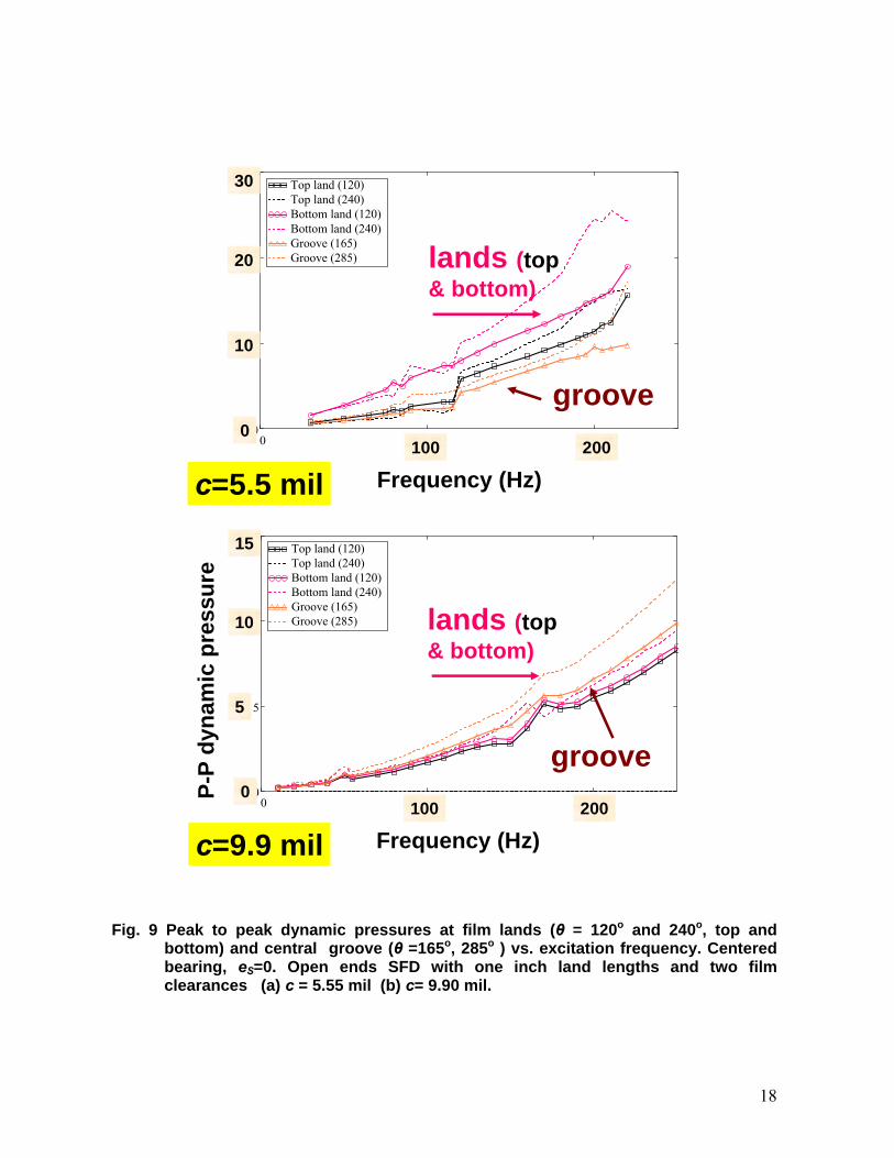
9 Peak to peak dynamic pressures at film lands (θ = 120o and 240o, top and bottom) and central groove (θ =165o, 285o ) vs. excitation frequency. Centered bearing, eS=0. Open ends SFD with one inch land lengths and two film clearances (a) c= 5.55 mil (b) c = 9.90 mil.

18

10 Ratio of groove to land peak-peak dynamic pressures vs. excitation frequency. Centered bearing, eS=0. Open ends SFD with one inch land lengths and two film clearances (a) c = 5.55 mil (b) c = 9.90 mil.

19

11 Open ends SFDs: Predicted pressure field for damper with one inch film land lengths and clearance clearances c~5.5 mil. Supply pressure 8.10 psi (0.55 bar).

22

12 Geometry and nomenclature for a model SFD with a central groove. Inset shows effective groove depth

23

13 Comparison of predicted and measured damping (CXX, CYY)SFD and inertia (MXX, MYY)SFD coefficients versus static eccentricity (eS). Open ends SFDs: radial clearances c~5.5 mil and 9.9 mil. Orbit radius amplitude r=0.5 mil. Predictions obtained with effective groove depth d=1.6c

25

A.1 Amplitude and phase angle of flexibility functions Gij vs. excitation frequency for lubricated test system. Experimental values and model curve fits. Identification range 120 – 230 Hz. Open ends damper with c=10mil and one inch land lengths. Centered journal (eS=0 mil), circular orbits r =0.5 mi

30

A.2 Estimated damping coefficients (CXX, CYY) and Im(H)/ vs. excitation frequency for open ends damper with c=10mil and one inch land lengths. Centered journal (eS=0 mil), circular orbits r =0.5 mil

30

A.3 Real and imaginary parts of direct impedances (HXX, HYY) vs. excitation frequency. Experimental data and fits using identified parameters. Open ends damper with c=10mil and one inch land lengths. Centered journal (eS=0 mil), circular orbits r =0.5 mil.

31

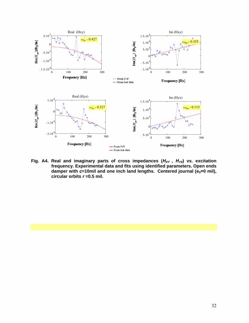
A.4 Real and imaginary parts of cross impedances (HXY, HYX) vs. excitation frequency. Experimental data and fits using identified parameters. Open ends damper with c=10mil and one inch land lengths. Centered journal (eS=0 mil), circular orbits r =0.5 mil.

32

A.5 Amplitude of flexibility functions Gij vs. excitation frequency for lubricated test system. Experimental values and model curve fits. Identification range 120 – 230 Hz. Open ends damper with c=10mil and one inch land lengths. Off-centered journal (eS=3 mil), circular orbits r =0.5 mil

33

A.6 Real and imaginary parts of direct impedances (HXX , HYY) vs. excitation frequency. Experimental data and fits using identified parameters. Open ends damper with c=10mil and one inch land lengths. Off-centered journal (eS=3 mil), circular orbits r =0.5 mil

33

A.7 Estimated damping coefficients (CXX, CYY) and Im(H)/ vs. excitation frequency for open ends damper with c=10mil and one inch land lengths. Off-centered journal (eS=3 mil), circular orbits r =0.5 mil.

34

A.8 Real and imaginary parts of cross impedances (HXY, HYX) vs. excitation frequency. Experimental data and fits using identified parameters. Open ends damper with c=10mil and one inch land lengths. Off-centered journal (eS=3 mil), circular orbits r =0.5 mil.

34

vi

C.1 Example of journal describing off-centered, large amplitude elliptical motion 38

C.2 Example of circular centered orbit analysis: journal motion X vs Y and SFD reaction forces (FX vs FY). Dots indicate discrete points at which code predicts SFD forces

39

1

shaker X

shaker YStatic loader

SFD

basesupport rods

Static loader

X

Y

shaker Xshaker Y

Static loader

SFD

basesupport rods

Static loader

X

Y

Significance of work High performance turbomachinery demands high shaft speeds, increased rotor flexibility,

tighter clearances in the flow passages, advanced materials, and increased tolerance to

imbalance [1]. Operation at high speeds induces severe dynamic loading with large amplitude

journal motions at the bearing supports. Squeeze Film dampers (SFD) aid to reduce rotor

vibrations due to imbalance and other sources and also serve to isolate the rotor(s) from the

engine frame or casing [2]. Energy efficient and reliable rotordynamic operation of aircraft

engines calls for detailed understanding of the forced performance in actual SFDs. Predictions

derived from classical SFD analyses fail to accurately predict the force coefficients for SFDs.

It is well known that classical lubrication formulas predict inertia force coefficients that are an

order of magnitude lesser than experimental data.

Pratt & Whitney Engines sponsored a two-

year experimental and computational program to

investigate novel SFD configurations operating at

typical conditions encountered in aircraft jet

engines. The project provided reliable SFD forced

performance data and benchmarked predictions

from a new computational program. The program

funded the construction of a high load SFD test

rig consisting of a rigid journal and an elastically supported bearing cartridge (BC). Two

electromagnetic shakers deliver periodic loads to the bearing to induce whirl motions at preset

amplitudes and frequencies; max. 500 lbf and 400 Hz. The test rig permits the excitation of the

BC with large amplitude whirl motions of arbitrary shape [3,4]. In practice this is a normal

occurrence. However, predicted (linear) SFD force coefficients may not represent with fidelity

the actual forced response of a SFD, in particular for off-centered journal motions.

Statement of work and budget

Recall that rotordynamic force coefficients

are strictly valid for infinitesimally small

amplitude motion about an equilibrium

condition. Both requirements, an equilibrium

X

Y

X

Y

X

Y

elliptical orbitscircular orbits

centered journal off-centered journal

2

state and small whirl amplitude motions, are often violated in SFD operation.

The proposed work is:

(a) Test the short length open ends damper with dynamic loads (20-300 Hz) inducing off-centered elliptical orbital motions with amplitude ratios as large as 5:1 to reach 80% of the bearing clearance (see inset).

(b) Extract SFD force coefficients from test impedances obtained over a frequency range and correlate coefficients with predictions of linear force coefficients and experimental coefficients for smallest whirl amplitudes (5%c).

(c) Perform computational model numerical experiments, similar to the physical tests, to also extract linearized SFD force coefficients from the nonlinear forces and valid within a frequency range. Determine the goodness of the linear-nonlinear representation from the equivalence in mechanical energy dissipation with the work performed from the actual nonlinear forces (experimental and numerical).

The TRC project was funded in December 2011 with the budget detail listed below. Mr. Sung-

Hwa Jung, M.S. graduate student, was hired as a Research Assistant (RA) with an effective

start date of January 1, 2012.

BUDGET FROM TRC FOR 2011-2012 Year ISupport for graduate student (20 h/week) x $ 1,800 x 12 months $ 21,600

Fringe benefits (0.6%) and medical insurance ($191/month) $ 2,419

Travel to (US) technical conference $ 1,200Tuition three semesters ($3,802 x 3) $ 10,138

Supplies for test rig $ 1,500Total Cost: $ 37,108

During the last 4 months, the RA has learned about the test rig components and operating

procedures, disassembled the test rig and installed, centered and aligned a journal to give a

SFD with a nominal 10 mil clearance and lands one inch long, and performed measurements

to identify the test system lubricated and dry force coefficients. To the end of May 2012, the

expenses amount to $13,687 which include the student salary ($1,950/month) plus social and

medical benefits and a modest amount for test rig expenses. For 2012-2013, the amount of

$14,000 is requested to continue the project until May 31, 2013.

The report describes the test rig and the measurements obtained by Paola Mahecha, a

former graduate student working with the SFD rig. In late April 2012, the current RA repeated

the same measurements, obtaining similar results and deriving identical conclusions.

Work will continue throughout 2012 and 2013 to complete the tasks outlined above, in

particular with large amplitude orbital motions to determine the validity of the common

impedance formulation to derive SFD force coefficients.

3

Description of large load SFD test rig Figure 1 shows the PW-SFD test rig and its support structure, a hydraulic static loader

and two electromagnetic shakers. Figure 2 depicts the test rig components and their

disposition, and Figure 3 presents a schematic view of the SFD test section and the lubricant

flow path. The SFD section is the gap between a stationary rigid journal and a bearing

cartridge (BC) elastically supported. The journal with diameter D=127 mm is rigidly mounted

to a base, which in turn is fastened to a heavy pedestal. Twelve steel rods (4 main rods and 8

flexural rods) support the BC to give an isotropic structural static stiffness (KS).

A hydraulic static loader positioned 45o away from the X and Y axes serves to statically

displace the BC to an off-centered or eccentric position. Two electromagnetic shakers

orthogonally positioned along the X and Y axes connect, through slender stingers, to the BC

for delivery of periodic loads at preset frequencies and amplitudes.

Static loader

Shaker assembly (Y direction)

Shaker assembly (X direction)

Static loader

Shaker in X direction

Shaker in Y direction

Test SFD

Top view

Isometric viewStatic loader

Shaker assembly (Y direction)

Shaker assembly (X direction)

Static loader

Shaker in X direction

Shaker in Y direction

Test SFD

Static loader

Shaker assembly (Y direction)

Shaker assembly (X direction)

Static loader

Shaker assembly (Y direction)

Shaker assembly (X direction)

Static loader

Shaker in X direction

Shaker in Y direction

Static loader

Shaker in X direction

Shaker in Y direction

Test SFD

Top view

Isometric view

Fig. 1 Top and side views of the PW SFD test rig.

4

in

Bearing Cartridge

Test Journal

Main support rod (4)

Journal BasePedestal

Piston ring seal

(location)

Flexural Rod (4, 8, 12)

Circumferential groove

Supply orifices (3)

Fig. 2. Cross-section view of test SFD with long journal. [3]

The journal is hollow to route lubricant from a supply system to the SFD through three

orifice restrictors, each 2.54 mm in diameter and 120o apart. When installed, the nominal

radial clearance between the journal and BC is c~0.025 mm (0.010 in). The BC with inner

diameter D+2c contains a groove of width and depth equal to LG=12.7 mm and dG=9.5 mm.

Hence, as shown in Figure 3, there are two squeeze film lands of length L=25.4 mm (1 in),

above and below the central groove.

Table 1 lists the dimensions of the damper and the measured radial clearance c~0.0251

mm (9.9 mil). Note that the groove depth is ~ 38 times the film thickness (clearance) in the

damper lands. The lubricant used is ISO VG 2 oil whose viscosity at room temperature is

similar to that of an aircraft jet engine lubricant at its operating condition (~ 200o C).

Note also that the number of active (open) orifice holes can be varied by selective

plugging. The journal incorporates end grooves for installation of piston seal rings, if needed.

Incidentally, the number of elastic rods supporting the BC can be varied from four to 16, and

thus the support stiffness can be tailored within a distinctive range, from KS=4.38 MN/m to

5

26.3 MN/m (25 klbf/in to 150 klbf/in). Presently, as depicted in Figure 4, twelve rods support

the BC.

Oil out, Qb

BaseSupportrod

Bearing Cartridge

Journal (D) Oil out, Qt

Oil in, Qin

Central groove

L½ L

L

End groove

End groove

Oil outOil collector

c

Oil out, Qb

BaseSupportrod

Bearing Cartridge

Journal (D) Oil out, Qt

Oil in, Qin

Central groove

L½ L

L

End groove

End groove

Oil outOil collector

BaseSupportrod

Bearing Cartridge

Journal (D) Oil out, Qt

Oil in, Qin

Central groove

L½ L

L

End groove

End groove

Oil outOil collector

c

Fig. 3 Cross section view of SFD test rig and lubricant flow path through damper film lands.

Table 1. Geometry and oil properties for test open ends SFD. Nominal radial clearance c=0.254 mm (10 mil).

SI unit US Unit Journal diameter, D 127 mm 5 inch Land length, L 25.4 mm 1 inch Radial clearance, c 0.251 mm 9.9 mil Groove axial length, LG 12.7 mm 0.5 inch depth, dG 9.5 mm 3/8 inch Oil wetted length, 2L+LG 63.5 mm 2.5 inch Groove static pressure, PG 0.11 bar 1.6 psig Oil inlet temperature, TS 23 oC 73 oF Lubricant ISO VG 2

Density, 785 kg/m3 49 lb/ft3

Viscosity at TS 0.0031 Pa.s 0.45 micro-Reynolds

Flow rate, Qin 5.00 LPM 1.32 GPM Max. static load (1.556 kN: 350 lbf),

Max. amplitude dynamic load (2,000 kN: 440 lbf) Range of excitation frequencies: 35-250 Hz

6

Fig. 4 Disposition of support rods holding bearing cartridge.

The test rig was constructed for a funded research program that aimed to deliver reliable

experimental SFD data and to develop an experimentally benchmarked and accurate SFD

forced performance predictive tool for integration in an engineering process handling the

rotordynamics design and analysis of jet engine performance. Several students, graduate and

undergraduate, worked in a fast paced project which delivered as intended in spite of the

severe economic crunch of the late 2000’s. The test schedule included dynamic load

measurements with two film two land lengths (short and long), four support stiffnesses, two

film radial clearances, and two end conditions (open and sealed).

The research team prepared 23 technical progress reports and comprehensive annual

reports. Near 1,500 dynamic load tests were conducted on short and long journals, with open

ends and sealed conditions for increasing static eccentricities, whirl amplitudes and

frequencies, lubricant feed pressure and varying the number of active feed holes. The bearing

dynamic motions imposed include unidirectional, circular and elliptical orbits. Note also that a

comprehensive LABview® DAQ system and a Mathcad® data post-processing code for

parameter identification were developed for the project.

Refs. [3, 4] are student M.S. theses relevant to the project. Seshaghiri [3] details the test

rig operation, parameter identification procedure, and reports SFD force coefficients for two

open ends configurations with two film land lengths, 0.5 inch and 1.0 inch. Mahecha [4]

continued the work and tested piston ring end sealed SFDs, extended the parameter

Retained flexural rod

Empty location

Main Support

X

Y

7

identification procedure, and showcased comparisons of her results with those for the open

ends SFD coefficients in Ref. [3]. San Andrés, Principal Investigator, developed the predictive

software for SFDs performing arbitrary orbital motions and based on earlier seminal work in

the Turbomachinery Laboratory [5,6]. Recently, San Andrés [7] compiled a technical paper

summing the test results in Ref. [3].

Identification of structural parameters for dry test system In general, upon installation and centering of a (new) journal or reconfiguration of the

rods’ support system the process calls for the measurement of the support structure static

stiffness (KS). To this end, static pull loads are imposed on the dry (unlubricated) structure

displacing the BC radially to a maximum eccentricity eS ~0.35c (3.5 mil).

Figure 5 shows the static load versus the BC displacement and the estimated static

structure stiffness KS~17.5 MN/m (100 klbf/in) from a linear curve-fit of the test data. Note

that the BC off-center displacement is 45o away from the X and Y axes.

0

100

200

300

400

0 0.5 1 1.5 2 2.5 3 3.5 4

static radial eccentricity, (mil)

stat

ic r

adia

l lo

ad (

lbf)

X

Y

e S

static load

e

c

45 deg

K S ~ 100 klbf/in

Fig. 5. Static pull load vs. BC radial displacement (eS). Bearing supported on 12 rods. Structure static stiffness KS~100 klbf/in

Still under dry (no lubricant) conditions and with a centered BC, single-frequency loads

are exerted on the BC to induce circular orbits of amplitude r=15.2 m (0.6 mil). The

8

dynamic loads F(t)={FX, FY}T , BC accelerations a(t)={aX, aY}T, and BC displacements

z(t)={x,y}T relative to the journal are recorded for each frequency () and processed for

estimation of the system parameters using an ad-hoc computational software implementing the

Instrument Variable Filter Method (IVFM ) [8].

In the frequency domain, the equations of motion of the unlubricated or dry test system are

2( ) ( ) ( )i s s s BCK C M z F M a (1)

where 1i , and for example ( ) ( )tDFT a a is the discrete Fourier transform of the

acceleration vector. Above (K, C, M)s stand for the matrices of structural force coefficients.

Note that 2( ) ( ) z a at excitation frequencies > 130 Hz [4]; hence the identification

method must treat the BC displacement z(t) and the acceleration a(t) as independent variables.

From Eq. (1), impedance coefficients Hs and flexibility coefficients Gs for the structure are

defined as

2 ,i -1s S s S s sH K M C G = H (2)

Table 2 lists the identified test (dry) system structural force coefficients from tests

spanning a frequency range of 50-210 Hz. Figure 6 depicts typical system flexibility

coefficients , ,,iij i j X Y

j

XG

F

(amplitude and phase) versus excitation frequency for circular

orbit tests conducted with an off-centered journal (eS=3 mil).

Table 2. Structural parameters of dry test system (bearing cartridge and support assembly) derived from circular centered orbits. Frequency range 50 Hz-210 Hz

Bearing Structure Direct XX Direct YY Cross XY Cross YX

Stiffness Ks [klbf/in] 107.3 120.1 -0.5 -0.4

Damping Cs [lbf-s/in] 8.4 8.8 0.0 -0.3

Mass Ms [lb] -3.8 -3.2 -0.3 0.4

System Mass MBC [lb] 48.0 48.0 Natural

frequency fns [Hz] 148 156

Damping ratio ξs 0.036 0.036 Static stiffness of structure KS = 100 klbf/in

9

The test results for the dry-structure evidence little structural cross-coupling, i.e.,

, ,XY YX XX YYs s s sK K K K Recall that the static structural stiffness KS=100 klbf/in while the

structural stiffnesses derived from the circular orbit tests ,XX YYs sK K are different.

XXsK and

YYsK are 7% and 20% higher that the static stiffness magnitude. The different stiffnesses also

cause a change in the natural frequencies of the dry-system structure.

0 100 200 3000

5 10 8

1 10 7

1.5 10 7

2 10 7

Magnitude:Gxx & Gxy vs. frequency

frequency (Hz)

fstart fend

0 100 200 3000

5 10 8

1 10 7

1.5 10 7

2 10 7

Magnitude: Gyy & Gyx vs. frequencyfstart fend

0 100 200 3004

2

0

2

4Phase angle: Fyx & Fyy vs frequency

frequency (Hz)

1.57

0 100 200 3004

2

0

2

4Phase angle: Fxy & Fxx vs frequency

frequency (Hz)

1.57

Fig. 6 Amplitude and phase angle of flexibility functions (Gij) vs. excitation frequency for dry (unlubricated) test system. Experimental values and model curve fits. Identification range 50 – 210 Hz. Open ends damper with c=9.9 mil and one inch land lengths. Off-centered journal (eS=3 mil), circular orbits r =0.5 mil.

10

Identification of force coefficients with lubricated test system Lubricant ISO VG 2 is supplied at an inlet pressure of

0.11 bar (1.6 psig) and temperature of ~73 oF (~23oC). The

recorded flow rate at this supply condition is ~1.32 GPM

(5.00 LPM). Flow rates for various other oil supply

pressures are listed later.

During tests with the BC at its centered position (eS=0)

and at three static eccentricities eS= 1, 2 and 3 mil (75 m)

displaced with the static loader, the dynamic load shakers

induced single frequency (50-250 Hz) circular orbits of the

BC with amplitude r=0.5 mil (12.5 m) , as shown in the

inset graph to the left. The BC static displacements (eS) are

45o away from the X and Y axes.

The equations of motion for the lubricated test system in the frequency domain become

2( ) ( ) ( )i S SFD S SFD S SFD SK + K C C M + M z F M a (3)

where (K, C, M)SFD represent the matrices of squeeze film damper force coefficients

(stiffness, damping and inertia).Eq. (3) can also be written as

( ) ( ) ( )( ) ( ) ( ) ( ) s SFD LUB SH + H z H z F M a (4)

where 2 i SFD SFD SFD SFDH K M C (5)

is the matrix of SFD impedance coefficients.

Table 3 lists the identified force coefficients for the lubricated test system, i.e., the

parameters add the SFD force coefficients to the dry-structure parameters. Cross-coupled

force coefficients are small, relative to the direct force coefficients, for most test conditions

except those with the largest static off-center BC displacement (eS=3 mil).

Appendix A shows characteristic flexibility coefficients , ,,iij i j X Y

j

XG

F

(amplitude and

phase) for the tests with the lubricated system. The appendix also presents the real and

imaginary parts of the impedance coefficients for scrutiny of the correlation between the

assumed physical model and the test data.

X

Y

r

eS

centered and off-centered circular orbits

11

Table 3. Force coefficients of lubricated test system from circular orbits: centered (eS=0) and three off-center positions (eS=1, 2 and 3 mil). Open ends SFD with c=9.90 mil and one inch land lengths. Frequency range 50 – 250 Hz

Identified Direct Coefficients

Static eccentricity

eS (mil) Static load

(lbf)

Whirl amplitude, r

(mil)

KXX (klbf/in)

KYY (klbf/in)

MXX (lb)

MYY (lb)

CXX (lbf-s/in)

CYY (lbf-s/in)

0.0 0 0.5 105.7 118.7 23.6 26.6 38.7 43.5 1.0 108 0.5 106.1 119.1 23.8 26.4 43.2 45.3 2.0 216 0.5 105.2 115.8 25.3 27.0 42.3 46.8 3.0 324 0.5 137.1 231.6 28.2 35.1 56.4 61.1

TABLE 2 DRY SYSTEM 107.3 120.8 -3.8 -3.2 8.4 8.8

Identified Cross-Coupled Coefficients

Static eccentricity

eS (mil) Static load

(lbf)

Whirl amplitude, r

(mil)

KXY (klbf/in)

KYX (klbf/in)

MXY (lb)

MYX (lb)

CXY (lbf-s/in)

CYX (lbf-s/in)

0.0 0 0.5 -1.7 -3.6 1.1 1.4 5.0 4.1 1.0 108 0.5 0.7 -3.9 1.2 0.6 6.8 7.1 2.0 216 0.5 0.0 -1.1 1.5 1.8 4.9 5.8 3.0 324 0.5 60.0 51.7 5.7 5.7 13.1 14.2

TABLE 2 DRY SYSTEM -0.5 -0.4 -0.3 0.4 0.0 -0.3

The experimental SFD force coefficients Table 4 gives the SFD coefficients derived by subtracting the dry system structural force

coefficients from the lubricated system force coefficients, i.e.

(K, C, M)SFD = (K, C, M)lubricated - (K, C, M)s (6)

Note that the reported SFD force coefficients represent the combined action of the two

parallel film lands (top and bottom) and the central groove. In general, the SFD cross-film

force coefficients are small relative to the direct force coefficients. Note also that CXX~CYY and

MXX~MYY, as expected from the circumferential symmetry of the test SFD system. In addition,

the SFD direct stiffnesses are a minute fraction of the test system structural stiffness.

However, the test results at eS=3 mil are suspect, i.e., the data results are anomalous. That is,

the assumed physical model (K, C, M) shows little correlation with the experimental data.

Refer to Appendix B for the uncertainty of the experimental force coefficients as well as the

12

goodness of the curve fits for the assumed physical model reproducing the experimental data

within a specific excitation frequency range.

Table 4. Open ends SFD force coefficients derived from circular orbits: centered (eS=0) and three off-center positions (eS=1, 2 and 3 mil). Frequency range 50 – 250 Hz. Damper with c=9.90 mil clearance and one inch land lengths.

SFD Direct Coefficients Static

eccentricity eS (mil)

Static load (lbf)

whirl amplitude,

r (mil) KXX (klbf/in)

KYY (klbf/in)

MXX (lb)

MYY (lb)

CXX (lbf-s/in)

MYY (lbf-s/in)

0.0 0 0.50 -1.6 -1.4 27.4 29.8 30.3 34.7

1.0 108 0.50 -1.2 -0.9 20.0 23.3 34.9 36.9

2.0 216 0.50 -2.1 -4.3 21.4 23.9 34.0 38.4

3.0 324 0.50 29.8 111.6 24.4 31.9 48.1 52.8

SFD Cross-Coupled Coefficients Static

eccentricity eS (mil)

Static load (lbf)

whirl amplitude,

r (mil) KXY (klbf/in)

KYX (klbf/in)

MXY (lb)

MYX (lb)

CXY (lbf-s/in)

CYX (lbf-s/in)

0.0 0 0.50 -1.2 -3.2 1.5 0.9 5.1 4.4

1.0 108 0.50 1.1 -3.5 1.6 0.2 6.8 7.4

2.0 216 0.50 0.4 -0.7 1.8 1.4 4.9 6.2

3.0 324 0.50 60.4 52.2 6.0 5.3 13.1 14.5

Comparison of force coefficients for two open ends SFDs, small and large clearances (c~5.5 and 9.9 mil)

Seshaghiri [3] reports the SFD force coefficients for two open ended dampers with film

land lengths equaling L= 0.5 inch and 1.0 inch and with a nominal clearance of 5 mil (actual

c=5.55 mil). Presently, the test results from Seshaghiri are compared against the present ones

obtained with a larger film clearance, c=9.90 mil, and identical film land lengths (L=25.4 mm

=1 inch).

For reference, Table 5 lists the distinct operation characteristics for the tests conducted

with the two dampers, both with same film length and differing film land clearances.

13

Table 5. Operating conditions for tests with open ends SFDs (one inch land lengths) and two film clearances

Actual clearance

c (mil)

Structure static stiffness

KS (klbf/in)

Whirl amplitude

r (mil)

Static Groove pressure

PG (psig)

Inlet flow rate

Qin (GPM)

Frequency range (Hz)

5.55 150 (*) 0.5 10.2 1.80 50-250

9.90 100 0.5 1.70 1.36 110-250

(*) The test SFD configuration in Ref. [3] had 16 rods in place to support the BC.

Figure 7 shows the SFD direct damping and inertia force coefficients versus static

eccentricity (eS) for two dampers with the same film length but differing clearances. Note that

the force coefficients are derived from circular orbit tests.

As expected, the damping and inertia force coefficients are larger for the damper with the

tightest clearance. The damping coefficients (CXX, CYY)SFD for the damper with small

clearance(c=5.5 mil) are ~3.7 times that for the large clearance (c=9.9 mil) damper. The added

mass coefficients (MXX, MYY)SFD appear to double when the clearance increases from c=5.5 to

9.9 mil.

For an open ends SFD with a centered journal, the classical damping (C*) and inertia (M*)

coefficients are [2]

3

* * *tanh

2 12π 12XX YY

LD DC C C L

LcD

(6)

3

* * *tanh

2 π 12XX YY

LL D DM M M

LcD

The formulas above are valid for a full film condition, i.e., without lubricant cavitation,

and for infinitesimally small amplitude journal motions. The predicted SFD force coefficients

using the formulas in Eq. (6) give

c=5.5 mil C* = 7,121 kNs/m (40.6 lbf.s/in) M* = 2.98 kg (6.58 lbm)

c=9.9 mil C* = 1,255 kNs/m (7.16 lbf.s/in) M* = 1.67 kg (3.69 lbm)

14

The theoretical force coefficients are a fraction of the identified coefficients, in particular

the added mass coefficients. The generation of fluid dynamic pressures in the central groove is

paramount to augment substantially the test SFD damping and inertia force coefficients.

From classical lubrication theory [2] for short length bearings damping coefficients are

proportional to (L/c)3 while added mass coefficients are proportional to (L/c). Since the

dampers’ film land lengths (L=1 inch) are identical, then the expected ratios for the force

coefficients are

3

5.55mil 5.55mil

9.90mil 9.90mil

9.90 9.901.78 ; 5.67

5.55 5.55c c

c c

M C

M C

(7)

From test results at the centered condition (eS=0); see Figure 7, the ratios of the added

masses and damping coefficients for the two dampers are

5.55mil 5.50mil

9.90mil 9.90mil

5.55mil 5.55mil

9.90mil 9.90mil

2.04; 1.70

3.86; 3.57

c c

c cXX YY

c c

c cXX YY

M M

M M

C C

C C

(8)

The test results show the added masses scale well with (1/c); however, the damping force

coefficients are not proportional to 1/c3. The rationale for the difference lies on the effect of

the central groove (and feed holes) on affecting the dynamic force coefficients. In other

words, the theory addresses to a simple damper model while the test damper has two

distinctive characteristics: three feed holes, 120o apart, and a deep central groove.

15

SFD (1 inch land lengths)

0

20

40

60

80

100

120

140

160

180

0.0 0.5 1.0 1.5 2.0 2.5 3.0 3.5

static eccentricity, e S (mil)

Da

mp

ing

co

effi

cie

nts

(lb

f -s/

in)

C SFD

circular orbits

C XX c= 9.9 mil

C YY c= 9.9 mil

C YY c= 5.5 mil

C XX c= 5.5 mil

 ~ 0.66g

l

P

P

~1.22g

l

P

P

0

10

20

30

40

50

60

70

80

0.0 0.5 1.0 1.5 2.0 2.5 3.0 3.5

static eccentricity, e S (mil)

Ad

ded

mas

s co

effi

cien

ts (

lb)

M SFD

M XX c= 9.9 mil

M YY c= 9.9 mil

M YY c= 5.5mil

M XX c= 5.5 mil

Fig. 7 Open ends SFDs: Direct damping (CXX, CYY)SFD and inertia (MXX, MYY)SFD coefficients versus static eccentricity (eS). Film radial clearances c~5.5 mil [3] and 9.9 mil. Orbit radius amplitude r=0.5 mil. One inch film land lengths.

The significant discrepancy between theoretical and experimental results is not unusual.

Please refer to prior relevant work by San Andrés [2] and Delgado and San Andrés [5] and

San Andrés and Delgado [6], and more recently the theses of Seshaghiri [3] and Mahecha [4].

16

Dynamic film pressures recorded in the film lands and groove of test damper

Figure 8 depicts the six piezoelectric pressure sensors installed in the bearing cartridge to

measure lubricant pressures at mid-axial length of the squeeze film lands and in the central

deep groove. In the top and bottom lands there are two pairs of sensors installed 120o apart.

Two other sensors measure dynamic pressures in the central groove. The sensor disposition

changes with the journal land lengths, one inch for the long damper and ½ inch for the short

one [3,4]. The sensors are flush mounted to the inner diameter of the bearing cartridge and

thus face directly into the film land or central groove.

This section presents the amplitude of peak-peak dynamic pressures recorded in the

damper central groove and in the film lands. During the dynamic load tests, the lubricant film

pressures are periodic with a fundamental frequency equaling that of the excitation frequency.

See Refs. [3,4] for more test data showing the time variation of the film and groove pressures.

Pressure sensor

Bottom Land

Pressure sensor locations

and

Central groove

and,

Central groove

Top Land

BC

25.4 mm

25.4 mm

Side view: Sensors located at middle plane of film lands

Top view: Sensors around bearing circumference

63.5 mm

12.7 mm

Pressure sensor

Pressure sensor

Pressure sensor

Bottom Land

Pressure sensor locations

and

Central groove

and,

Central groove

Top Land

BC

25.4 mm

25.4 mm

Side view: Sensors located at middle plane of film lands

Top view: Sensors around bearing circumference

63.5 mm

12.7 mm

Pressure sensor

Pressure sensor

Fig. 8 Disposition of dynamic pressure sensors in bearing cartridge. Damper with one inch lands lengths.

17

For the open ends SFDs with film clearances c=9.9 mil and c=5.5 mil, Figure 9 illustrates

the effect of excitation frequency on the peak to peak (p-p) dynamic pressures recorded in the

film lands (Pl), top and bottom, and in the central groove (Pg) at two circumferential locations.

The p-p film pressures for the damper with the small clearance are more than twice larger than

those for the damper with the large clearance. Note that the groove dynamic pressures are not

negligible.

The measurements demonstrate that the deep central groove does not isolate adjacent film

lands and is not a region of constant pressure! In actuality, the measurements make evident

that the dynamic pressures in the central groove are as substantive as those in the film lands.

In actuality, for the damper with the larger clearance (c=9.9 mil), the dynamic pressures in the

groove are even higher than those in the film lands. The effect is evident in Figure 10 that

shows the ratio of groove to film land peak to peak pressures (Pg/Pl) versus excitation

frequency.

18

0 100 2000

10

20

30Top land (120)Top land (240)Bottom land (120)Bottom land (240)Groove (165)Groove (285)

Frequency (Hz)

100 200

30

20

10

0

c=5.5 mil

groove

lands (top & bottom)

0 100 2000

5

10

15Top land (120)Top land (240)Bottom land (120)Bottom land (240)Groove (165)Groove (285)

Frequency (Hz)

P-P

dyn

amic

pre

ssu

re

100 200

15

10

5

0

c=9.9 mil

groove

lands (top & bottom)

Fig. 9 Peak to peak dynamic pressures at film lands (θ = 120o and 240o, top and bottom) and central groove (θ =165o, 285o ) vs. excitation frequency. Centered bearing, eS=0. Open ends SFD with one inch land lengths and two film clearances (a) c = 5.55 mil (b) c= 9.90 mil.

19

0 100 2000

1

2

3

4Top land (120)Top land (240)

Frequency (Hz)

P-P

pre

ssu

re r

atio

s

100 2000

c=5.5 mil

groovelands (top)

1.0

0 100 2000

1

2

3

4Top land (120)Top land (240)

Frequency (Hz)

P-P

pre

ssu

re r

atio

s

100 200

1.0

c=9.9 mil

groovelands (top)

Fig. 10 Ratio of groove to land peak-peak dynamic pressures vs. excitation frequency. Centered bearing, eS=0. Open ends SFD with one inch land lengths and two film clearances (a) c = 5.55 mil (b) c = 9.90 mil.

20

Measurements of flow rate and flow conductances For the two open ends SFDs, clearances c=5.55 mil and c= 9.90 mil, Table 6 lists the

measured lubricant flow rates at the damper inlet (Qin) and through the bottom land flow (Qb)

for increasing magnitudes of the static pressure recorded in the central groove (PG). Note that

for a perfectly centered and aligned damper BC and with a uniform clearance Qb/Qin=0.50.

The table also lists the flow conductances, i.e., the ratio of flow rate to pressure drop across a

film land, Cc=Q/PG.

Table 6. Measured lubricant flow rates (inlet and through bottom land) and static

pressure in central groove for two open ends dampers with film clearances (a) c=9.9 mil (b) c=5.5 mil [3]. One inch film land lengths.

a) c=9.90 mil b) c=5.5 mil PG Qin Qb Ratio PG Qin Qb Ratio

psig GPM GPM b/in psig GPM GPM b/in 1.50 1.18 0.64 0.54 6.5 1.2 0.6 0.50 1.70 1.36 0.77 0.56 8.1 1.5 0.7 0.47

2.1 1.76 0.98 0.56 10.2 1.8 0.8 0.44 Flow GPM/psi 0.814±0.02 0.453 0.56 Conductance GPM/psi 0.181±0.02 0.084 0.47

As expected, the damper with a larger clearance “leaks” more than the SFD with a tighter

clearance. This damper has a lesser flow resistance or higher flow conductance, C~0.45

GPM/psi, while the damper with small clearance has C~0.08 GPM/psi for the bottom film

lands. The ratio of flow conductances (large/small clearances) is ~5.4.

On the other hand, for a simple or idealized damper with film length (L) and with uniform

feed pressure on one end and ambient pressure on the other end, the axial flow conductance

(C) is [2]

3 1

12

Q DcC

P L

(9)

From the Eq. above, theory delivers a ratio of flow conductances

3

9.90mil

5.55mil

9.905.65

5.55c

c

C

C

, similar in magnitude to that of the measurements.

However, using the simple formula in Eq. (9) delivers poor predictions for the measured

flow rates; that is Cc=9.9mil=0.735 GPM/psi and Cc=5.55mil=0.129 GPM/psi. Compare these

magnitudes against the measured values, C~0.453 GPM/psi for the large clearance damper

21

and C~0.084 GPM/psi for the small clearance damper. Hence, simple theory predicts a larger

flow conductance (lesser flow resistance) than the measurements evidence. Clearly the

difference is attributed to the flow resistance in the central groove and the uneven pressure

distribution since there are three supply holes. Note that for both dampers, the ratio

Ctest/Ctheory~0.65.

Even when adding the groove ½ axial length in Eq. (9), i.e., with L=1.25 in, the

predictions render a slight decrease in flow conductance and Ctest/Ctheory~0.78. Thus, the

measured flow conductances, lesser than simple theory predicts, are due to the flow

interactions in the central groove.

Using a computational model that accounts for the central groove and feed holes [9], the

PI conducted a parametric study on effective groove depths to match the recorded flow rates

and thus obtaining identical flow conductances. The analysis requires of an effective groove

depth d=1.6c [6] to predict similar flow conductances, i.e., C~0.452 GPM/psi for the large

clearance damper, and C~0.080 GPM/psi for the small clearance damper.

The required effective groove depths, a little deeper than the actual film clearance,

demonstrate that the feed groove has a significant flow resistance; in direct opposition to the

common assumption of a flow source (negligible flow resistance). For reference, Figure 11

shows the predicted static pressure field for a centered damper with the small clearance. Note

that the pressure in the groove section varies circumferentially from one feed hole to the next.

In the film land, the pressure drops linearly towards the ambient condition; however, the

upstream condition at the interface with the edge of the central groove is largely affected by

the holes disposition and effective groove depth.

22

1

9

17

25

33

41

49

57

65

73

81

89S

1

S8

0.00

0.10

0.20

0.30

0.40

0.50

0.60

circ coordinate (node #)

axial coordinate

0.5-0.6

0.4-0.5

0.3-0.4

0.2-0.3

0.1-0.2

0.0-0.1

Inner Film

Pressure

Feed hole (3 x 120 deg)

groove

land

z

Pressure (bar)

1

9

17

25

33

41

49

57

65

73

81

89S

1

S8

0.00

0.10

0.20

0.30

0.40

0.50

0.60

circ coordinate (node #)

axial coordinate

0.5-0.6

0.4-0.5

0.3-0.4

0.2-0.3

0.1-0.2

0.0-0.1

Inner Film

Pressure

Feed hole (3 x 120 deg)

groove

land

z

Pressure (bar)

Fig. 11. Open ends SFDs: Predicted pressure field for damper with one inch film land lengths and clearance clearances c~5.5 mil. Supply pressure 8.10 psi (0.55 bar).

Predictions of SFD force coefficients and comparisons to test data San Andrés and Delgado [5,6] advance a sound physical bulk-flow model for prediction

of the pressure film in thin film land sections separated by grooves, as shown in Fig. 12. The

model bridges the gap between extensive experimental data1 in oil seal rings and SFDs and

simple model predictions that ignore the flow field in grooved regions. The finite element

analysis solves numerically the modified Reynolds equation

2

3 3 2

212

P P h hh h h

R R z z t t

(9)

1 The test data shows force coefficients much larger than classical model predictions; thus the need for a more accurate development. Please see Refs. [5,6] for a comprehensive review of the literature, the foundation of the model, and comparisons of predictions to archival test data. In 2012, the ASME –IGTI Structures and Dynamics Division gave a Best Paper Award to Ref. [6].

23

where h and P are the fluid film thickness and film pressure in the lubricated flow region

120 2 ,0 Gz L L . Above µ and ρ are the lubricant viscosity and density, respectively.

The modified Reynolds equation above accounts for temporal fluid inertia effects. The film

thickness is

( ) ( )( ), ,

cos sint tz X Yz t

h c e e

(10)

where c(z) is a step-wise clearance distribution along the axial direction and (eX, eY) are the

components of the instantaneous journal center eccentricity.

z

LLG

do

Bearing

Journal

End seal

c : clearance

Lubricant in

Lubricant out

orifice

groove

film land

dG

D, diameter

Lubricant in

recirculationzone

Effective groove depth

streamline

Lubricant out

separation line

d

Lubricant in

recirculationzone

Effective groove depth

streamline

Lubricant out

separation line

d

Fig. 12. Geometry and nomenclature for a model SFD with a central groove. Inset shows effective groove depth [6].

As per Refs. [5,6], a groove effective depth (d) lesser than the physical depth (dG) is

needed to predict accurately SFD force coefficients. Presently, as depicted in Fig. 12, the

effective depth d=1.6c ( 8.88 mil and 15.84 mil) for both dampers is based on a close

matching of the predicted flow rate to the measured flow magnitudes.

Recall the experimental force coefficients are derived from small amplitude (r=0.5 mil)

circular orbits about a static eccentricity (eS), 45o away from the X, Y axes. Presently,

predictions are obtained for perturbations of the journal center about the equilibrium position.

Figure 13 shows a comparisons of the current predictions for direct damping and inertia force

coefficients and the experimental force coefficients (see Fig. 7) versus static eccentricity for

the dampers with a small and large clearances, c=5.55 mil and c=9.9 mil. The graphs also

display the theoretical force coefficients based on the classical lubrication equations, See Eqs.

(6).

24

The comparisons show that the current computational model [10] does a good job in

predicting accurate force coefficients. Notice the large difference between the current

predictions and test data and the magnitudes predicted by the simple classical lubrication

formulas. The discrepancies are due to the flow interaction in the central groove and which

generate a large dynamic pressure field.

The model predicts for the large clearance damper: larger inertia coefficients and lesser

damping coefficients than the test values. On the other hand, for the small clearance SFD, the

model predicts more damping and less inertia coefficients than the experimental results. The

discrepancies may be due to the constant value of effective groove depth selected for the

analysis and also because the effect of the feed holes is not properly accounted for when the

damper describes circular orbits.

25

0

20

40

60

80

100

120

140

160

180

200

0.0 0.5 1.0 1.5 2.0 2.5 3.0 3.5 4.0

static ccentricity, e S (mil)

Dam

pin

g c

oef

fici

ents

(lb

f -s/

in)

C SFD

C XX c= 9.9 mil

C YY c= 9.9 mil

C YY c= 5.5 mil

C XX c= 5.5 mil

lines - predictions

symbols: test data

classical theory (7.1 lbf.s/in)

classical theory (40.6 lbf.s/in)

0

10

20

30

40

50

60

70

80

0.0 0.5 1.0 1.5 2.0 2.5 3.0 3.5 4.0

static eccentricity, e S (mil)

Ad

ded

mas

s co

effi

cien

ts (

lb)

M SFD

M XX c= 9.9 mil

M YY c= 9.9 mil

M YY c= 5.5mil M XX c= 5.5 mil

lines - predictions

symbols: test data

classical theory (3.7 - 6.6 lb)

Fig. 13. Comparison of predicted and measured damping (CXX, CYY)SFD and inertia (MXX, MYY)SFD coefficients versus static eccentricity (eS). Open ends SFDs: radial clearances c~5.5 mil and 9.9 mil. Orbit radius amplitude r=0.5 mil. Predictions obtained with effective groove depth d=1.6c

26

Conclusions Note: The project received funding in December 2011, effectively starting on January 1, 2012.

The report describes the components and operation of a large load SFD test rig, details

measurements of dynamic loads conducted on a large clearance (c=9.9 mil) open ends,

centrally grooved SFD, and presents the experimental SFD force coefficients for operation at

three static eccentric positions. The damper consists of two parallel film lands, one inch in

length, separated by a deep central groove, ½ inch in width. Three equally spaced holes, 120o

apart, supply an ISO VG 2 lubricant into the central groove at room temperature.

The experimental SFD force coefficients are compared to test results obtained earlier with

the same damper but with a smaller clearance (c=5.5 mil) [3] and against predictions obtained

from an advanced physical model that includes the flow field in the central groove and the

interaction with the adjacent film lands [10]. Dynamic pressures recorded in the film lands

(top and bottom) and in the central groove reveal that the central groove does not isolate the

adjacent film lands but actually is a region where dynamic pressures are as large as in the film

lands. This phenomenon is presently the rule rather than the exception as abundant test data in

the laboratory and practice attest [5-7].

The measurements show negligible cross-coupled force coefficients since the orbital

motions are of small amplitude (r=0.5 mil ~ 0.05c) albeit the excitation frequencies are as

large as 250 Hz and with large amplitude dynamic forces (~ 90 lbf).

The experimental squeeze films damping and stiffness coefficients are much larger than

predictions obtained from classical lubrication theory [2]. For example, at the centered (es=0)

and largest static eccentricity (es=3 mil), the force coefficients extracted from the dynamic

load measurements, the advanced predictive model [10], and those based on classical

lubrication are listed below:

Centered bearing KXX

(klbf/in) KYY

(klbf/in) MXX (lb)

MYY (lb)

CXX (lbf-s/in)

MYY (lbf-s/in)

Experimental -1.6 -1.4 27.4 29.8 30.3 34.7

Perturbation analysis [10]

0.00 0.00 22.2 22.2 26.3 26.3

Orbital analysis, App C 0.07 0.07 22.2 22.2 26.3 26.3

Classical Lubrication, Eqs. (6)

0.0 0.0 3.19 3.19 7.16 7.16

27

Off-centered 3 mil KXX

(klbf/in) KYY

(klbf/in) MXX (lb)

MYY (lb)

CXX (lbf-s/in)

MYY (lbf-s/in)

Experimental -1.6 -1.4 27.4 29.8 30.3 34.7

Perturbation analysis [10]

0.060 0.071 25.7 27.7 25.4 28.2

Orbital analysis, App C 0.061 0.071 25.8 27.5 24.3 26.7

Classical Lubrication, Eqs. (6)

NA NA

Hence, the open ends centrally grooved damper delivers ~3.5 times more damping than

the classical formula predicts and generates a ~7.4 larger added mass. The measurements thus

reveal the limited applicability of the classical formulas and make pathetic the need to use a

more advanced model to predict accurately the dynamic forced of SFDs in practice.

The experimental force coefficients for the large clearance damper are also compared

against prior experimental results for an identical damper (diameter and length) but with a

smaller clearance, c=5.5 mil [3]. The experimental results show the added masses scale well

with (1/c); however, the damping force coefficients are not proportional to 1/c3. The ratio of

damping force coefficients for the small and large clearance dampers is ~3.80 while the scale

law (1/c3) gives 5.68. The discrepancy is due to the generation of an uneven static pressure

field in the groove region as determined by the disposition of the lubricant feed holes.

Appendix C details the orbital analysis model implemented in an updated version of the

computational model described in Ref. [10]. The novel analysis will deliver more accurate

force coefficients representative of actual SFD orbital paths.

28

Nomenclature a(t) {aX, aY}T Vector of bearing accelerations [m/s2]

( )a ( )tDFT a Discrete Fourier transform of accelerations [m/s2]

c Film land clearance [m] C Damping coefficient [N.s/m] Cc Q/P. Flow conductance [LPM/Pa] dG Groove depth [m] d Effective groove depth [m] D Journal diameter [m], R= ½ D eS Static eccentricity (along 45o) [m] eX, eY Dynamic eccentricity components [m] fn Natural frequency [rad/s] F(t) {FX, FY}T Vector of dynamic loads [N]

( )F ( )tDFT F Discrete Fourier transform of accelerations [m/s2]

G H-1. Flexibility matrix [m/N] H 2 i K M C . Matrix of impedance coefficients [N/m] i 1 . Imaginary unit K Stiffness coefficient [N/m] KS Support stiffness [N/m] M Mass coefficient [kg] MBC Bearing cartridge mass [kg] L Film land length [m] LG Grove width [m] Qin Flow rate [LPM] Qb Flow rate through bottom land [LPM] P Film pressure [Pa] PG Static oil pressure in central groove [Pa] Pl, Pg Dynamic pressures in film land and central groove [Pa] r Circular orbit amplitude [m] t Time [s] X,Y Coordinate axes z(t) {x,y}T Vector of bearing displacements relative to journal [m]

( )z ( )tDFT z Discrete Fourier transform of bearing displacements [m]

Damping ratio [-] x/R. Circumferential coordinate [rad] Oil density [kg/m3] and viscosity [Pa.s] Excitation frequency [rad/s] Subscripts

s Structure LUB Lubricated system SFD Squeeze film damper

29

References [1] Zeidan, F., San Andrés, L., and Vance, J.M., 1996, “Design and Application of Squeeze

Film Dampers in Rotating Machinery,” Proc. of the 25th Turbomachinery Symposium, Turbomachinery Laboratory, Texas A&M University, pp. 169-188, September, Houston.

[2] San Andrés, L., 2010, "Squeeze Film Dampers: Operation, Models and Technical Issues," Modern Lubrication Theory, Notes 13, Texas A&M University Digital Libraries, https://repository.tamu.edu/handle/1969.1/93197

[3] Seshaghiri, S., 2011, “Identification of Force Coefficients in Two Squeeze Film Dampers with a Central Groove,” M.S. Thesis, Texas A&M Univ., College Station, TX., USA.

[4] Mahecha, P., 2011, “Experimental Dynamic Forced Performance of a Centrally Grooved, End Sealed Squeeze Film Damper,” M.S. Thesis, Texas A&M Univ., College Station, TX., USA.

[5] Delgado, A., and San Andrés, L., 2010, “A Model for Improved Prediction of Force Coefficients in Grooved Squeeze Film Dampers and Grooved Oil Seal Rings”, ASME Journal of Tribology, 132(July), p. 032202 (1-12)

[6] San Andrés, L., and Delgado, A., 2012, “A Novel Bulk-Flow Model for Improved Predictions of Force Coefficients in Grooved Oil Seals Operating Eccentrically,” ASME J. Eng. Gas Turbines Power, 134(May), p. 052509 (1-10)

[7] San Andrés, L., 2012, “Damping And Inertia Coefficients for Two Open Ends Squeeze Film Dampers with a Central Groove: Measurements and Predictions,” ASME Paper GT2012-6212 (accepted for publication at ASME J. Eng. Gas Turbines Power)

[8] San Andrés, L., 2009, Modern Lubrication Theory, “Experimental Identification of Bearing Force Coefficients,” Notes 14, Texas A & M University Digital Libraries, http://repository.tamu.edu/handle/1969.1/93197

[10] San Andrés, L., 2010, "PW_SFD_2010," SFD Predictive Code Developed for Pratt & Whitney Engines, MEEN Dept., Texas A&M University, Proprietary

30

Appendix A. Sample of flexibility and impedance functions for lubricated test system (a) Tests at centered condition, eS= 0 mil

0 100 200 3000

5 10 8

1 10 7

1.5 10 7

2 10 7

Magnitude:Gxx & Gxy vs. frequency

frequency (Hz)

fstart fend

0 100 200 3000

5 10 8

1 10 7

1.5 10 7

2 10 7

Magnitude: Gyy & Gyx vs. frequencyfstart fend

0 100 200 3004

2

0

2

4Phase angle: Fxy & Fxx vs frequency

frequency (Hz)

1.57

0 100 200 3004

2

0

2

4Phase angle: Fyx & Fyy vs frequency

frequency (Hz)

1.57

Fig. A1 Amplitude and phase angle of flexibility functions Gij vs. excitation frequency

for lubricated test system. Experimental values and model curve fits. Identification range 120 – 230 Hz. Open ends damper with c=10mil and one inch land lengths. Centered journal (eS=0 mil), circular orbits r =0.5 mil.

0 100 200 3000

50

100

Im(H)/w

cyy_US

fstart fend

0 100 200 3000

20

40

60

Im(H)/w

cxx_US

fstart fend

Fig. A2 Estimated damping coefficients (CXX, CYY) and Im(H)/ vs. excitation frequency

for open ends damper with c=10mil and one inch land lengths. Centered journal (eS=0 mil), circular orbits r =0.5 mil.

31

0 100 200 3002 105

1 105

0

1 105

2 105

Real (Hxx)fstart fend

0 100 200 3000

2 104

4 104

6 104

8 104

Im (Hxx)fstart fend

rxxre 0.995

rxxIm 0.939

0 100 200 3002 105

1 105

0

1 105

2 105

Real (Hyy)fstart fend

0 100 200 3000

2 104

4 104

6 104

8 104

1 105

Im (Hyy)fstart fend

ryyre 0.993

ryyIm 0.916

Fig. A3 Real and imaginary parts of direct impedances (HXX , HYY) vs. excitation frequency. Experimental data and fits using identified parameters. Open ends damper with c=10mil and one inch land lengths. Centered journal (eS=0 mil), circular orbits r =0.5 mil.

32

0 100 200 3001.5 104

1 104

5 103

0

5 103

Real (Hxy)

0 100 200 3001 104

5 103

0

5 103

1 104

1.5 104

Im (Hxy)

Im(H

xy)

[lb

f / i

n]

rxyre 0.427rxyIm 0.355

0 100 200 3002 104

1 104

0

1 104

Real (Hyx)

Re(

Hyx

) [

lbf

/ in]

0 100 200 3005 103

0

5 103

1 104

1.5 104

Im (Hyx)

Im(H

yy)

[lb

f / i

n]ryxre 0.327 ryxIm 0.115

Fig. A4. Real and imaginary parts of cross impedances (HXY , HYX) vs. excitation

frequency. Experimental data and fits using identified parameters. Open ends damper with c=10mil and one inch land lengths. Centered journal (eS=0 mil), circular orbits r =0.5 mil.

33

(b) Tests at off-centered displacement eS= 3 mil

0 100 200 3000

5 10 8

1 10 7

1.5 10 7

2 10 7

Magnitude:Gxx & Gxy vs. frequency

frequency (Hz)

fstart fend

0 100 200 3000

5 10 8

1 10 7

1.5 10 7

2 10 7

Magnitude: Gyy & Gyx vs. frequencyfstart fend

Fig. A5 Amplitude of flexibility functions Gij vs. excitation frequency for lubricated test

system. Experimental values and model curve fits. Identification range 120 – 230 Hz. Open ends damper with c=10mil and one inch land lengths. Off-centered journal (eS=3 mil), circular orbits r =0.5 mil.

0 100 200 3002 105

1 105

0

1 105

2 105

Real (Hxx)fstart fend

0 100 200 3000

5 104

1 105

1.5 105

Im (Hxx)fstart fend

rxxre 0.899rxxIm 0.639

0 100 200 3001 105

0

1 105

2 105

3 105

Real (Hyy)fstart fend

0 100 200 3000

5 104

1 105

1.5 105

Im (Hyy)fstart fendryyre 0.92

ryyIm 0.168

Fig. A6 Real and imaginary parts of direct impedances (HXX , HYY) vs. excitation

frequency. Experimental data and fits using identified parameters. Open ends damper with c=10mil and one inch land lengths. Off-centered journal (eS=3 mil), circular orbits r =0.5 mil.

34

0 100 200 3000

50

100

150

Im(H)/w

cxx_US

fstart fend

0 100 200 3000

50

100

Im(H)/w

cyy_US

fstart fend

Fig. A7. Estimated damping coefficients (CXX, CYY) and Im(H)/ vs. excitation frequency

for open ends damper with c=10mil and one inch land lengths. Off-centered journal (eS=3 mil), circular orbits r =0.5 mil.

0 100 200 3000

5 104

1 105

1.5 105

Real (Hxy)

0 100 200 3001 104

0

1 104

2 104

3 104

4 104

Im (Hxy)Im

(Hxy

) [

lbf

/ in]

rxyre 0.309rxyIm 1.893 10

3

0 100 200 3002 104

2 104

6 104

1 105

Real (Hyx)

Re(

Hyx

) [

lbf

/ in]

0 100 200 3000

2 104

4 104

6 104

Im (Hyx)

Im(H

yy)

[lb

f / i

n]ryxre 0.349 ryxIm 0.221

Fig. A8 Real and imaginary parts of cross impedances (HXY , HYX) vs. excitation

frequency. Experimental data and fits using identified parameters. Open ends damper with c=10mil and one inch land lengths. Off-centered journal (eS=3 mil), circular orbits r =0.5 mil.

35

Appendix B. Uncertainty and goodness of fit for estimated force coefficients

Table B.1 list the uncertainties for the identified physical parameters (stiffness, damping

and inertia) and the goodness of fit with the physical (K-C-M) model. This table complements

the identified force coefficients in Table 4, pg. 12. Refs. [3,4] give details on the uncertainty

analysis.

In general the uncertainties for all the parameters are a small fraction (5% or less) of the

magnitude reported. For the tests with BC static eccentricity eS= 0, 1 and 2 mil, the goodness

of fit, R2~0.95 and higher, denotes the physical parameters (K, C, M)XX,YY represent very well

the experimentally derived impedances. On the other hand for the case eS=3 mil, the goodness

of fit are too low thus indicating the physical model does not represent the experimental data

with any accuracy.

Table B1. Open ends SFD lubricated test system: Uncertainty and goodness of fit for force coefficients. From tests at various BC eccentric positions (eS=1, 2 and 3 mil). Circular orbits with amplitude r=0.5 mil, frequency range 50 – 250 Hz. Film land clearance c=9.9 mil and one inch land lengths

Direct coefficients Goodness of fit

UKXX UKYY UMXX UMYY UCXX UCYY Static

eccentricity (mil) (klbf/in) (klbf/in) (lb) (lb) (lbf-s/in) (lbf-s/in)

Re (XX)

Re (YY)

Im (XX)

Im (YY)

0.0 1.7 1.9 0.7 0.8 0.8 0.9 0.995 0.993 0.939 0.916

1.0 1.7 1.9 0.7 0.7 0.9 1.0 0.889 0.977 0.637 0.823

2.0 1.6 1.8 0.7 0.8 0.9 1.0 0.987 0.993 0.969 0.960

3.0 2.1 3.6 0.8 1.0 1.2 1.2 0.899 0.920 0.639 0.168

Cross coupled coefficients Goodness of fit

UKXY UKYX UMXY UMYX UCXY UCYX Static

cccentricity (mil) (klbf/in) (klbf/in) (lb) (lb) (lbf-s/in) (lbf-s/in)

Re (XY)

Re (YX)

Im (XY)

Im (YX)

0.0 0 -0.1 0 0 0.4 0.4 0.427 0.327 0.355 0.1151.0 0 -0.1 0 0 0.4 0.4 0.112 0.018 0.066 0.0182.0 0 0 0 0.1 0.4 0.4 0.411 0.340 0.344 0.3023.0 0.9 0.8 0.2 0.2 0.5 0.5 0.306 0.283 0.003 0.237

36

Small amplitude motions

-1.0

-0.8

-0.6

-0.4

-0.2

0.0

0.2

0.4

0.6

0.8

1.0

-1.0 -0.8 -0.6 -0.4 -0.2 0.0 0.2 0.4 0.6 0.8 1.0

X/c

Y/c

e

Appendix C. Estimation of bearing force coefficients from orbital paths

Fluid film bearing analytical models and computational programs predict rotordynamic

force coefficients for a specified static equilibrium eccentricity (see inset). The mechanical

parameters, hereby labeled as the true (linear) force coefficients, represent the idealization of

infinitesimally small amplitude journal motions about an static position or equilibrium

eccentricity ,e ex y .

Fluid film bearing reaction forces F={FX, FY}T relate to journal center motions

( ) ( ),t e t ex x x y y x by

e

e

XX XX XY XX XY XX XY

Y YX YY YX YY YX YYY

FF K K C C M Mx x x

F K K C C M MF y y y

(C.1)

or ( t ) eF = F -KΔz -CΔz -MΔz (C.2)

where Fe is the bearing static reaction force vector at the

equilibrium position (xe, ye). Above, the matrices K, C and

M contain the stiffness, damping and inertia force

coefficients, respectively. Fluid inertia or added

coefficients (M) are significant in squeeze film dampers

and seals with dense fluids operating at high speeds and

with large pressure differentials. In general, the force

coefficients for liquid (incompressible fluid) bearings or

seals are frequency independent; thus, the physical K-C-M

model is quite adequate. However, bearings or seals handling compressible fluids (gases)

show force coefficients that depend strongly on the frequency () of whirl motion; hence,

K=K() and C= C(). Incidentally, bearings with compliant surfaces or moving parts, such as

tilting pad bearings, also show strong frequency effects in their dynamic forced response.

Recall that the (linear) force coefficients represent changes in bearing reaction forces to

small amplitude motions about an equilibrium position; that is

37

, , ,

; ;e e e e e e

X Y XXY YX XX

x y x y x y

F F FK C M

y x x

(C.3)

for example. The mathematical formulation calls for infinitesimally small motions; however,

engineering use and practice show these coefficients to be valid in producing bearing reaction

forces with journal whirl motions of sizable amplitudes. Often, the applicability of a

theoretical formulation goes well beyond rigorous mathematical definitions.

The archival literature, every so often, presents studies2 that question the validity of the

linearized force representation, Eq. (C.1), and embark on non-linear analyses to assess

(quantify) the error in using the linearized formulation as opposed to a “more exact” model

derived from a Taylor-series expansion of the forces; say,

( )

2 32 3

2 3

2 3 22 3

2 3

2 32 3

2 3

1 1.....

2! 3!

1 1..... .....

2! 3!

1 1.....

2! 3!

t e

X X XX X

e e e

X X X X

e e e e

X X X

e e e

F F FF F x x x

x x x

F F F Fy y y x y

y x yy y

F F Fx x x

x x x

2 3 22 3

2 3

1 1..... ..... ....

2! 3!X X X X

e e e e

F F F Fy y y x y

y x yy y

(C.4)

which leads to both linear and nonlinear force coefficients. Clearly, the question is when to

truncate the nonlinear model so as to keep its accuracy while ensuring some degree of

computational efficiency. This question is perhaps irrelevant in an age of fast computing

where engineering processes can readily integrate the complete nonlinear bearing model into a

predictive environment and simply calculate at each time (step),

( )

( )

( ) ( ), , , , ,t

t

X

t tY

Fx y x y x y

F

f (C.5)

2 Tieu, A.K., and Qiu, Z.L., 1995, “Stability of Finite Journal Bearings–-from Linear and Nonlinear Bearing

Forces,” Trib. Trans., v. 38, pp. 627-635. Braun, MJ, and Hu, Y., 1991, “Nonlinear Effects in a Plain Journal Bearing: Part

1—Analytical Study; Part 2—Results,” ASME J. Tribol., 113, pp. 555–570.

38

SFDs often experience orbital (elliptical) motions with large amplitudes, thus violating the

major assumption to derive linearized rotordynamic force coefficients. Presently, an existing

computational model [10] also performs an orbit analysis to predict instantaneous reaction

forces (FX, FY) for a specified journal motion with arbitrary amplitudes of motion and static

position. The model assumes single frequency () motions3 of the type

( ) ( ) ( )

( ) ( ) ( )

cos( ) sin( )

sin( ) cos( )

t S X t Y t

t S X t Y t

x x a a

y y a a

(C.6)

where ( ) ( )cos( ), sin( )X t X Y t Ya r t a r t (C.7)

Above ,S Sx y denote the components of the static eccentricity vector, ,X Yr r are the

amplitudes of motion along the X,Y axes, is a phase angle, and is the angle of the ellipse

axis with the X coordinate. Figure C.1 depicts a typical off-centered journal orbital motion

with ,S Sx y =0.3c, 40.2 , 0.3 , 0andX Yr c r c .

Orbit

-1.0

-0.8

-0.6

-0.4

-0.2

0.0

0.2

0.4

0.6

0.8

1.0

-1.0 -0.8 -0.6 -0.4 -0.2 0.0 0.2 0.4 0.6 0.8 1.0

X/c

Y/c

Fig. C.1 Example of journal describing off-centered, large amplitude elliptical motion

Figure C.2 depicts a typical example of an orbital analysis conducted with a large amplitude

circular centered orbit. The motion path is specified and the damper reaction forces predicted at

discrete points along the orbital path during a full period of whirl motion.

3 The whirl frequency is positive, i.e. counter-clockwise as per the graph.

39

X

Y Y

X

lbf

Forces

mil

Journal orbit

Fig. C.2 Example of circular centered orbit analysis: journal motion X vs Y and SFD reaction forces (FX vs FY). Dots indicate discrete points at which code predicts SFD forces

The SFD instantaneous reaction force superimposes a dynamic force to a static force, i.e.

F=Fstatic+Fdyn. The dynamic component of the SFD reaction force is modeled in a linearized

form as

dyn SFD SFD SFDF K z C z + M z (C.8)

where z is a vector of dynamic displacements and (K, C, M)SFD are matrices of stiffness,

viscous damping and inertia force coefficients. From Eq. (C.6), z is given by the real part of

cos( ) sin( ) i t i tX Y

Y X

r i re e

i r r

1z z (C.9)

where Tc cx y1z . The dynamic or time varying part of the reaction force is periodic with

fundamental period T=2/Using Fourier series decomposition, the damper dynamic

reaction force Fdyn can be decomposed as

2 31 ....i t i t i te e e dyn II IIIF F F F (C.10)

To satisfy Eq. (C.8), one must approximate the reaction force as

1

i te dynF F (C.11)

40

This approximation is valid for small amplitude motions and nearly centered operating

conditions4. Substitution of Eqs. (C.11) and (C.9) into Eq. (C.8) gives

21 i SFD SFD SFD 1 1F K M C z H z (C.12)

with H as a matrix of damper impedances, 2 i SFD SFD SFDH K M C . Eq. (C.12)

provides two equations for determination of four impedance coefficients. Hence, in the

numerical simulation, an orbital path with the same amplitudes is specified but with a negative

frequency, <0 (clockwise whirl motion).

Next, the computational program calculates the SFD time varying reaction force for the

new orbital path and delivers the fundamental Fourier components of motion and forces, i.e. z2

and F2. The specified orbital paths (forward and backward whirl orbits) ensure linear

independence of the two reaction forces. Thus, using the two sets of results, write Eq. (C.12)

as

1 2 1 2F F H z z (C.13)

at a particular frequency, say k. Thus,

1

1 2k 1 2H F F z z (C.14)

delivers the impedance coefficients HXX, HYY, HXY, HYX at k. The analysis stacks impedances

for a set of frequencies (k=1,2,….N) from which, by linear curve fits, one determines

2 Re

Im

SFD SFD

SFD

K M H

C H (C.15)

Note that the numerical analysis follows an identical procedure as in the experimental

identification of the test data. The computer program developed can be thought as a virtual

tool to perform parameter identification in SFDs.

The goodness of the orbit-analysis derived SFD parameters is determined from the energy

dissipated over one cycle of whirl motion. That is, over one period (T=2), the work

performed by the SFD reaction force is

c X YT

W F x F y dt Tdx F (C.12)

4 The validity of the assumption will be verified later with more examples as well as benchmarking against test data.

41

Using the linearized model, 1; i testatic dyn dynF F F F F ,

c S dynW dt dt dt W W T T Tstatic dyn static dynz F F z F z F (C.13)

The work performed by the static components of the bearing force is nil, i.e.

0S S S SS X Y X YW dt F x F y dt F x dt F y dt T

staticz F (C.14)

since the whirl motion describes a full closed orbit with , i t i tc cx x e y y e .

Using the estimated linear force coefficients, the work is

_ 1~dyn linearW dt dt T TSFD SFD SFDz F z K z +C z + M z (C.15)

The ratio _dyn linear

c

WW will provide a measure of how well the estimated linear model

reproduces the actual work (energy dissipated).

Further analysis and correlation to the experimental measurements will appear in the

coming months.