60

Lecture 5. NEWTON’S LAWS OF MOTION

Newton’s Laws of Motion

Law 1. Unless a force is applied to a particle it will eitherremain at rest or continue to move in a straight line atconstant velocity,

Law 2. The acceleration of a particle in an inertial referenceframe is proportional to the force acting on the particle, and

Law 3. For every action (force), there is an equal andopposite reaction (force).

Newton’s second Law of Motion is a Second-Order DifferentialEquation

where is the resultant force acting on the particle, is theparticle’s acceleration with respect to an inertial coordinatesystem, and m is the particle’s mass.

61

Figure 3.1 A car located in the X, Y (inertial) system by IX anda particle located in the x, y system by ix.

A particle in the car can be located by

The equation of motion,

is correct. However,

because the x, y system is not inertial.

62

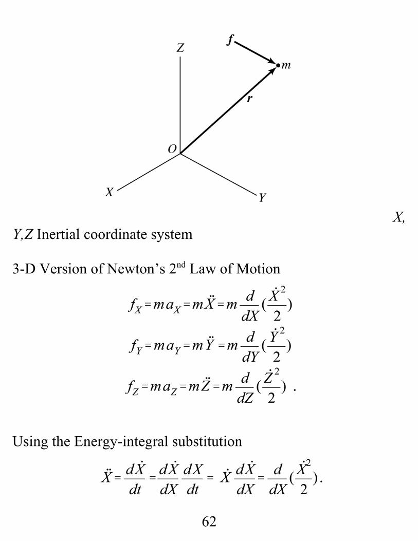
X,Y,Z Inertial coordinate system

3-D Version of Newton’s 2nd Law of Motion

Using the Energy-integral substitution

63

Multiplying the equations by dX, dY, dZ , respectively, and adding gives

This “work-energy” equation is an integrated form of Newton’ssecond law of motion . The expressions are fullyequivalent and are not independent.

The central task of dynamics is deriving equations of motion forparticles and rigid bodies using either Newton’s second law ofmotion or the work-energy equation.

64

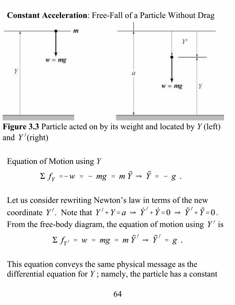
Figure 3.3 Particle acted on by its weight and located by Y (left)and (right)

Constant Acceleration: Free-Fall of a Particle Without Drag

Equation of Motion using Y

Let us consider rewriting Newton’s law in terms of the newcoordinate . Note that .From the free-body diagram, the equation of motion using is

This equation conveys the same physical message as thedifferential equation for Y ; namely, the particle has a constant

65

acceleration downwards of g, the acceleration of gravity.

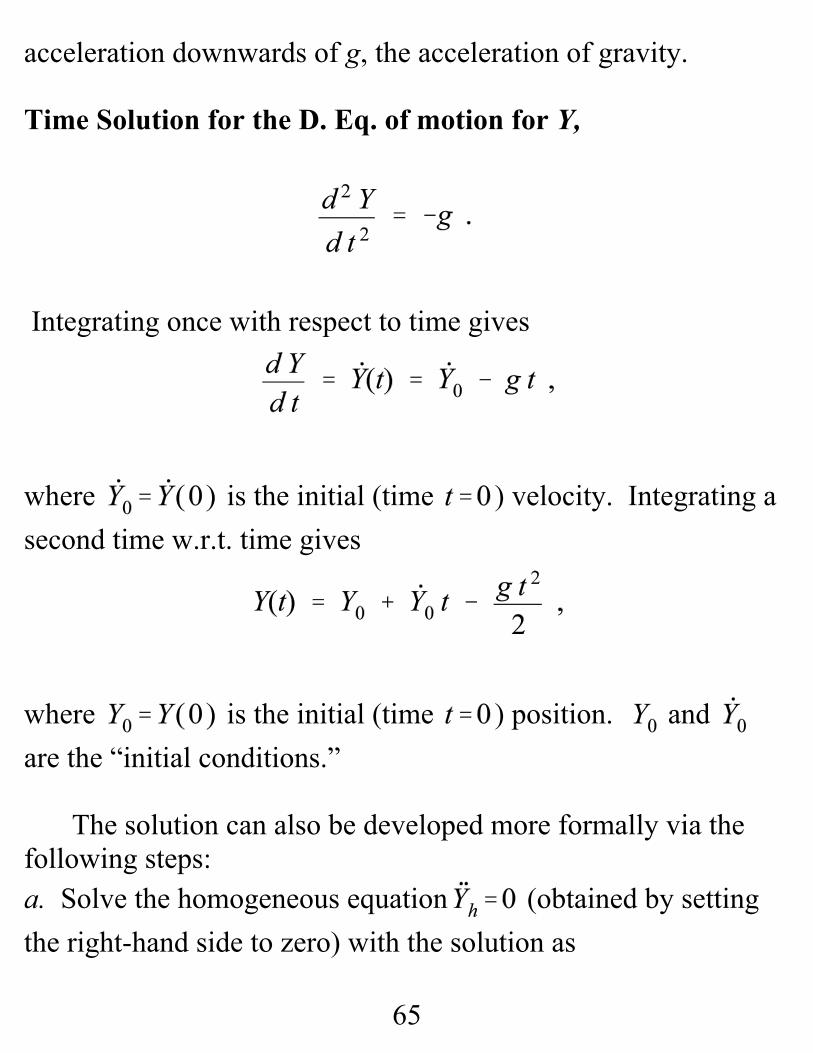
Time Solution for the D. Eq. of motion for Y,

Integrating once with respect to time gives

where is the initial (time ) velocity. Integrating asecond time w.r.t. time gives

where is the initial (time ) position. and are the “initial conditions.”

The solution can also be developed more formally via thefollowing steps:a. Solve the homogeneous equation (obtained by settingthe right-hand side to zero) with the solution as

66

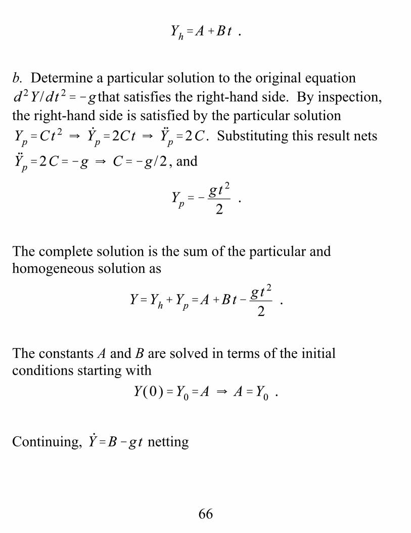
b. Determine a particular solution to the original equationthat satisfies the right-hand side. By inspection,

the right-hand side is satisfied by the particular solution. Substituting this result nets

, and

The complete solution is the sum of the particular andhomogeneous solution as

The constants A and B are solved in terms of the initialconditions starting with

Continuing, netting

67

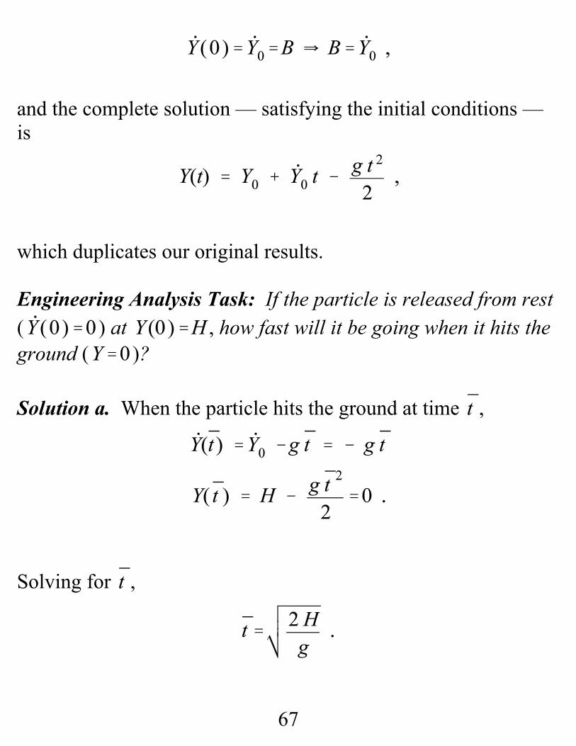
and the complete solution — satisfying the initial conditions —is

which duplicates our original results.

Engineering Analysis Task: If the particle is released from rest( ) at , how fast will it be going when it hits theground ( )?

Solution a. When the particle hits the ground at time ,

Solving for ,

68

Solving for ,

Solution b. Using the energy-integral substitution,

changes the differential equation to

Multiplying through by dY and integrating gives

Since , is

Solution c. There is no energy dissipation; hence, we can workdirectly from the conservation of mechanical energy equation,

69

where is the kinetic energy. The potential energy ofthe particle is its weight w times the vertical distance above ahorizontal datum. Choosing ground as datum gives and

The weight is a conservative force, and in the differentialequation is , pointing in the direction. Strictly speaking,a conservative force is defined as a force that is the negative ofits gradient with respect to a potential function V. For thissimple example, with

Hence (as noted above) the potential energy function for gravityis the weight times the distance above a datum plane; i.e.,

70

Figure 3.5 (a) Particle being held prior to release, (b) Ycoordinate defining m’s position below the release point, ( c)Spring reaction force

Acceleration as a Function of Displacement: Spring Forces

Particle suspended by a spring and acted on by its weight. Thespring is undeflected at ; i.e., (zero springforce). The spring force has a sign that is the oppositefrom the displacement Y, and it acts to restore the particle to theposition .

71

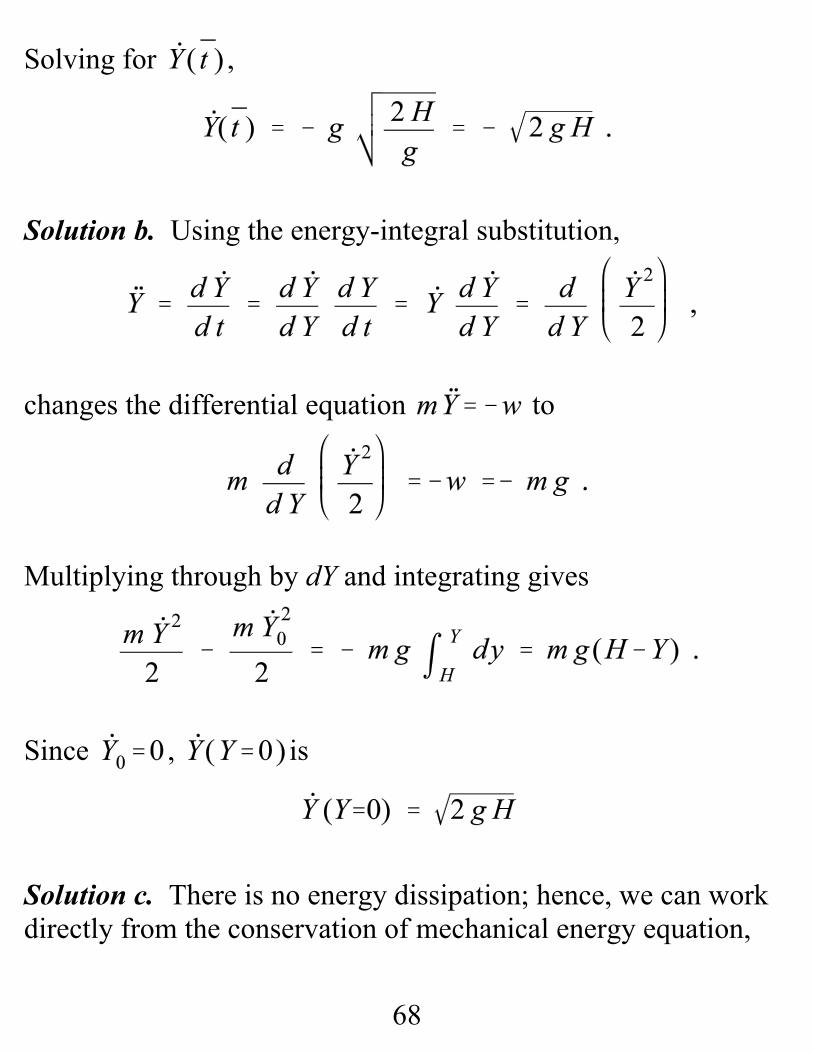
Figure 3.5 (d) Free-bodydiagram for , (e) Free-bodydiagram for

(3.13)

From the free-body diagram of figure 3.5d, Newton’s second lawof motion gives the differential equation of motion,

Figure 3.5d-e shows that for and

72

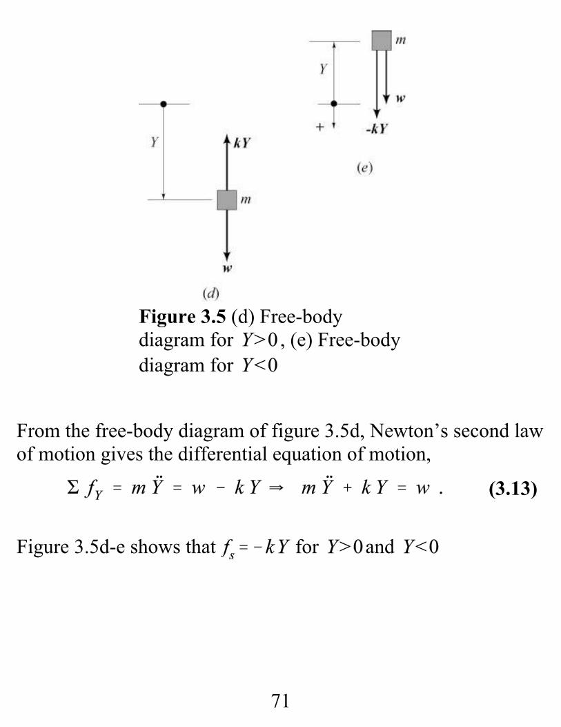
Figure 3.5 (a) Mass m inequilibrium, (b) Equilibrium free-body diagram, (c) General-positionfree-body diagram

Deriving the Equation of Motion for Motion about Equilibrium

Figure 3.5c applies for m displaced the distance y below theequilibrium point. The additional spring displacement generatesthe spring reaction force , and yields the followingequation of motion.

(3.14)

73

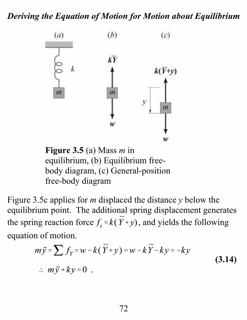
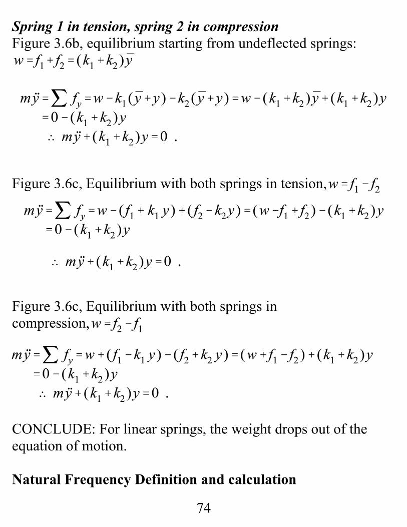
Figure 3.6 (a) Equilibrium, (b)Equilibrium with spring 1 in tension andspring 2 in compression, (c) Equilibriumwith both springs in tension, (d)Equilibrium with both springs incompression

This result holds for a linear spring and shows that w iseliminated, leaving only the perturbed spring force ky.

MOREEQUILIBRIUM, 1 MASS - 2SPRINGS

74

Spring 1 in tension, spring 2 in compressionFigure 3.6b, equilibrium starting from undeflected springs:

Figure 3.6c, Equilibrium with both springs in tension,

Figure 3.6c, Equilibrium with both springs incompression,

CONCLUDE: For linear springs, the weight drops out of theequation of motion.

Natural Frequency Definition and calculation

75

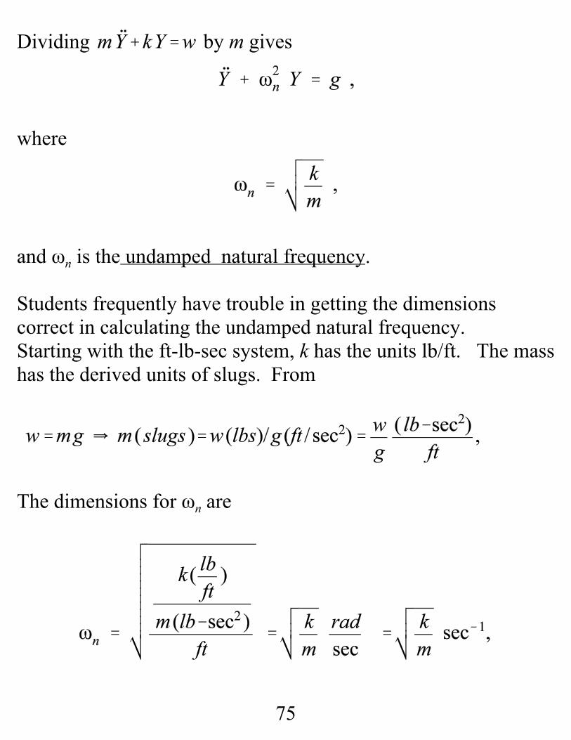
Dividing by m gives

where

and ωn is the undamped natural frequency.

Students frequently have trouble in getting the dimensionscorrect in calculating the undamped natural frequency. Starting with the ft-lb-sec system, k has the units lb/ft. The masshas the derived units of slugs. From

,

The dimensions for ωn are

76

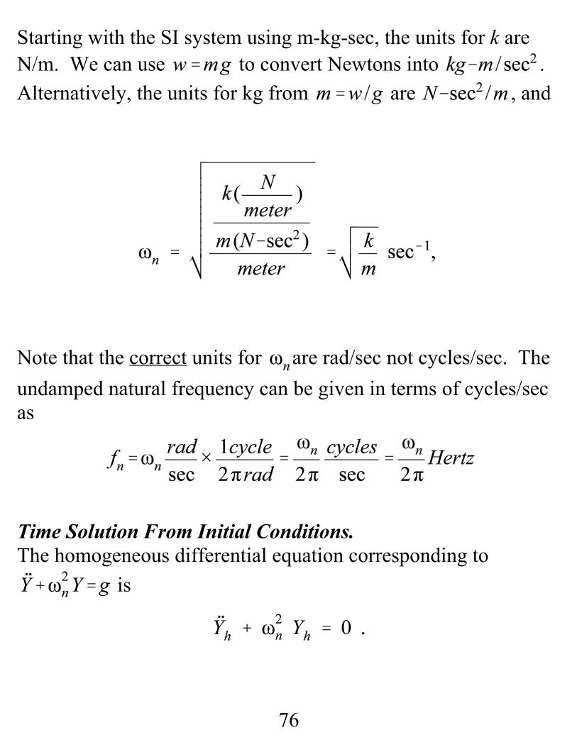
Starting with the SI system using m-kg-sec, the units for k areN/m. We can use to convert Newtons into . Alternatively, the units for kg from are , and

Note that the correct units for are rad/sec not cycles/sec. Theundamped natural frequency can be given in terms of cycles/sec as

Time Solution From Initial Conditions.The homogeneous differential equation corresponding to

is

77

Substituting the guessed yields

Guessing yields the same result; hence, the generalsolution is solution

The particular solution is

Note that this is also the static solution; i.e.,. The complete solution is

For the initial conditions , the constant Ais obtained as

78

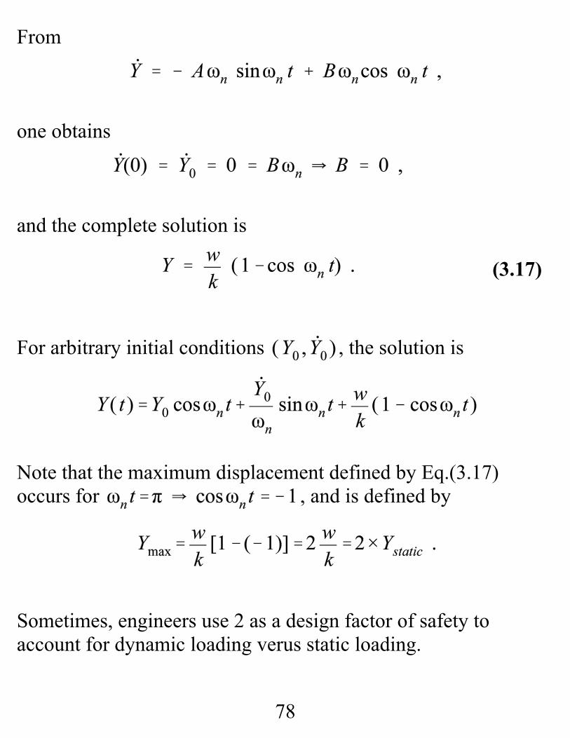
(3.17)

From

one obtains

and the complete solution is

For arbitrary initial conditions , the solution is

Note that the maximum displacement defined by Eq.(3.17)occurs for , and is defined by

Sometimes, engineers use 2 as a design factor of safety toaccount for dynamic loading verus static loading.

79

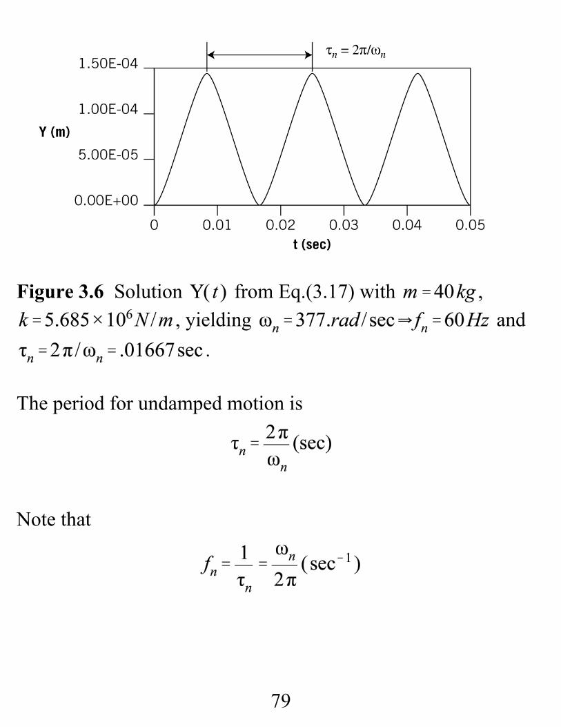
Figure 3.6 Solution from Eq.(3.17) with ,, yielding and

.

The period for undamped motion is

Note that

80

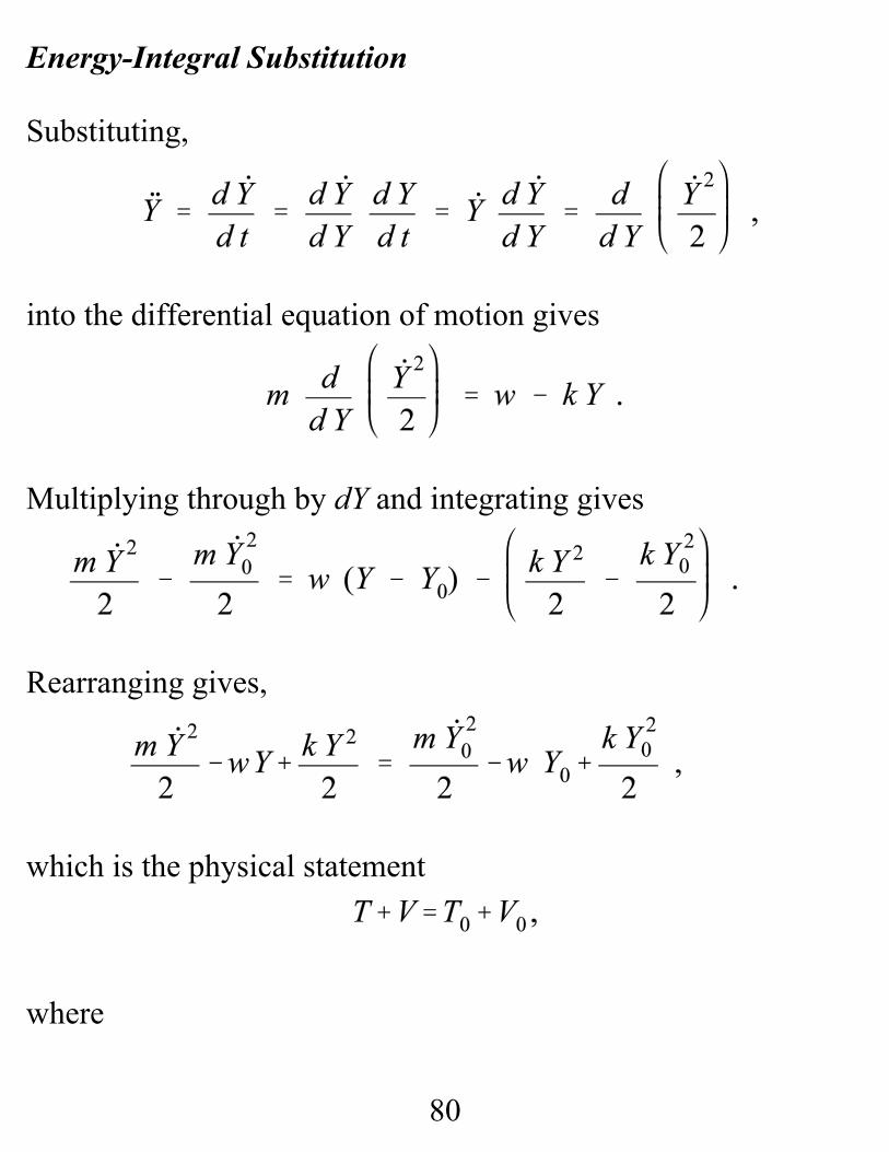
Energy-Integral Substitution

Substituting,

into the differential equation of motion gives

Multiplying through by dY and integrating gives

Rearranging gives,

which is the physical statement

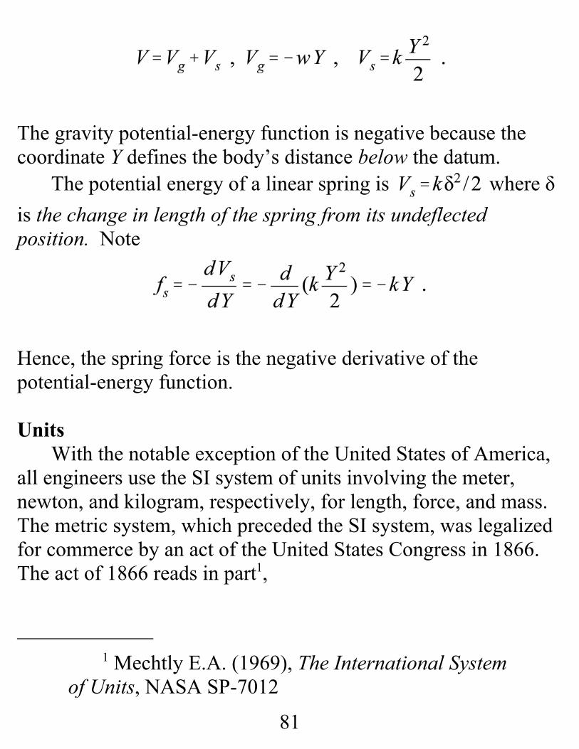
where

1 Mechtly E.A. (1969), The International Systemof Units, NASA SP-7012

81

The gravity potential-energy function is negative because thecoordinate Y defines the body’s distance below the datum.

The potential energy of a linear spring is where δis the change in length of the spring from its undeflectedposition. Note

Hence, the spring force is the negative derivative of thepotential-energy function.

UnitsWith the notable exception of the United States of America,

all engineers use the SI system of units involving the meter,newton, and kilogram, respectively, for length, force, and mass. The metric system, which preceded the SI system, was legalizedfor commerce by an act of the United States Congress in 1866. The act of 1866 reads in part1,

82

It shall be lawful throughout the United States of America toemploy the weights and measures of the metric system; andno contract or dealing or pleading in any court, shall bedeemed invalid or liable to objection because the weights ormeasures referred to therein are weights or measures of themetric system.

None the less, in the 21st century, USA engineers, manufacturers,and the general public continue to use the foot and pound asstandard units for length and force. Both the SI and US systemsuse the second as a unit of tim. The US Customary system ofunits began in England, and continues to be referred to in theUnited States as the “English System” of units. However, GreatBritain adopted and has used the SI system for many years.

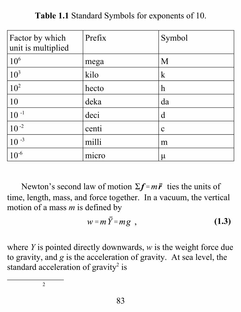
Both the USA and SI systems use the same standard symbolsfor exponents of 10 base units. A partial list of these symbols isprovided in Table 1.1 below. Only the “m = -3” (mm = millimeter = 10-3m) and “k = +3” ( km = kilometer = 103 m)exponent symbols are used to any great extent in this book.

2

83

(1.3)

Table 1.1 Standard Symbols for exponents of 10.

Factor by whichunit is multiplied

Prefix Symbol

106 mega M103 kilo k102 hecto h10 deka da10 -1 deci d10 -2 centi c10 -3 milli m10-6 micro μ

Newton’s second law of motion ties the units oftime, length, mass, and force together. In a vacuum, the verticalmotion of a mass m is defined by

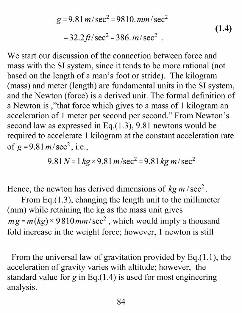
where Y is pointed directly downwards, w is the weight force dueto gravity, and g is the acceleration of gravity. At sea level, thestandard acceleration of gravity2 is

From the universal law of gravitation provided by Eq.(1.1), theacceleration of gravity varies with altitude; however, thestandard value for g in Eq.(1.4) is used for most engineeringanalysis.

84

(1.4)

We start our discussion of the connection between force andmass with the SI system, since it tends to be more rational (notbased on the length of a man’s foot or stride). The kilogram(mass) and meter (length) are fundamental units in the SI system,and the Newton (force) is a derived unit. The formal definition ofa Newton is ,”that force which gives to a mass of 1 kilogram anacceleration of 1 meter per second per second.” From Newton’ssecond law as expressed in Eq.(1.3), 9.81 newtons would berequired to accelerate 1 kilogram at the constant acceleration rateof , i.e.,

Hence, the newton has derived dimensions of .From Eq.(1.3), changing the length unit to the millimeter

(mm) while retaining the kg as the mass unit gives, which would imply a thousand

fold increase in the weight force; however, 1 newton is still

85

(1.5)

required to accelerate 1 kg at ,and

Hence, for a kg-mm-second system of units, the derived forceunit is 10-3 newton = 1 mN (1 milli newton).

Another view of units and dimensions is provided by theundamped-natural-frequency definition of a mass Msupported by a linear spring with spring coefficient K . Perturbing the mass from its equilibrium position causesharmonic motion at the frequency , and ’s dimension is

, or sec-1 (since the radian is dimensionless) .Using kg-meter-second system for length, mass, and time, thedimensions for follow from

confirming the expected dimensions. Shifting to mm for the length unit while continuing to use

the newton as the force unit would change the dimensions of thestiffness coefficient K to and reduce K by a factor of1000. Specifically, the force required to deflect the spring 1 mm

86

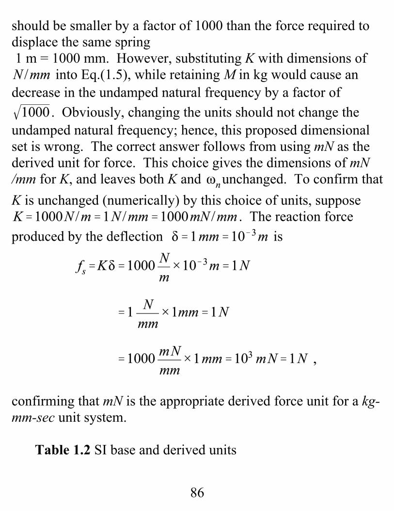
should be smaller by a factor of 1000 than the force required todisplace the same spring 1 m = 1000 mm. However, substituting K with dimensions of

into Eq.(1.5), while retaining M in kg would cause andecrease in the undamped natural frequency by a factor of

. Obviously, changing the units should not change theundamped natural frequency; hence, this proposed dimensionalset is wrong. The correct answer follows from using mN as thederived unit for force. This choice gives the dimensions of mN/mm for K, and leaves both K and unchanged. To confirm thatK is unchanged (numerically) by this choice of units, suppose

. The reaction forceproduced by the deflection is

confirming that mN is the appropriate derived force unit for a kg-mm-sec unit system.

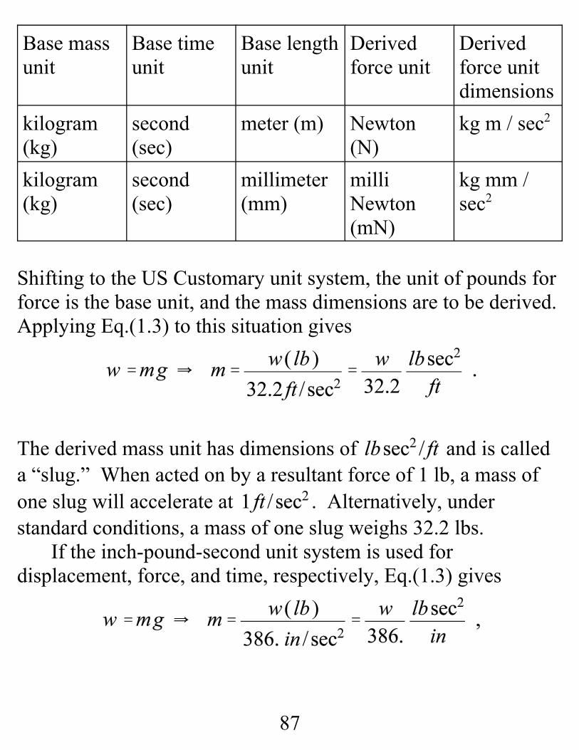
Table 1.2 SI base and derived units

87

Base massunit

Base timeunit

Base lengthunit

Derivedforce unit

Derivedforce unitdimensions

kilogram(kg)

second(sec)

meter (m) Newton(N)

kg m / sec2

kilogram(kg)

second(sec)

millimeter(mm)

milliNewton(mN)

kg mm /sec2

Shifting to the US Customary unit system, the unit of pounds forforce is the base unit, and the mass dimensions are to be derived. Applying Eq.(1.3) to this situation gives

The derived mass unit has dimensions of and is calleda “slug.” When acted on by a resultant force of 1 lb, a mass ofone slug will accelerate at . Alternatively, understandard conditions, a mass of one slug weighs 32.2 lbs.

If the inch-pound-second unit system is used fordisplacement, force, and time, respectively, Eq.(1.3) gives

88

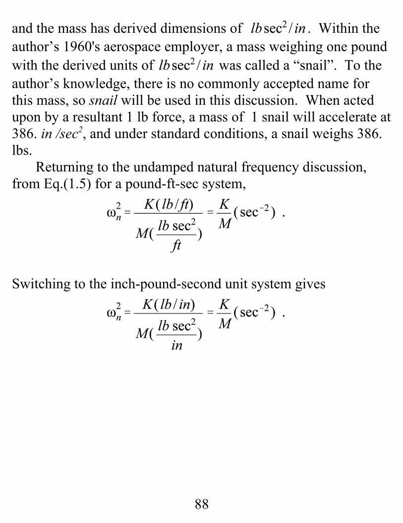
and the mass has derived dimensions of . Within theauthor’s 1960's aerospace employer, a mass weighing one poundwith the derived units of was called a “snail”. To theauthor’s knowledge, there is no commonly accepted name forthis mass, so snail will be used in this discussion. When actedupon by a resultant 1 lb force, a mass of 1 snail will accelerate at386. in /sec2, and under standard conditions, a snail weighs 386.lbs.

Returning to the undamped natural frequency discussion,from Eq.(1.5) for a pound-ft-sec system,

Switching to the inch-pound-second unit system gives

89

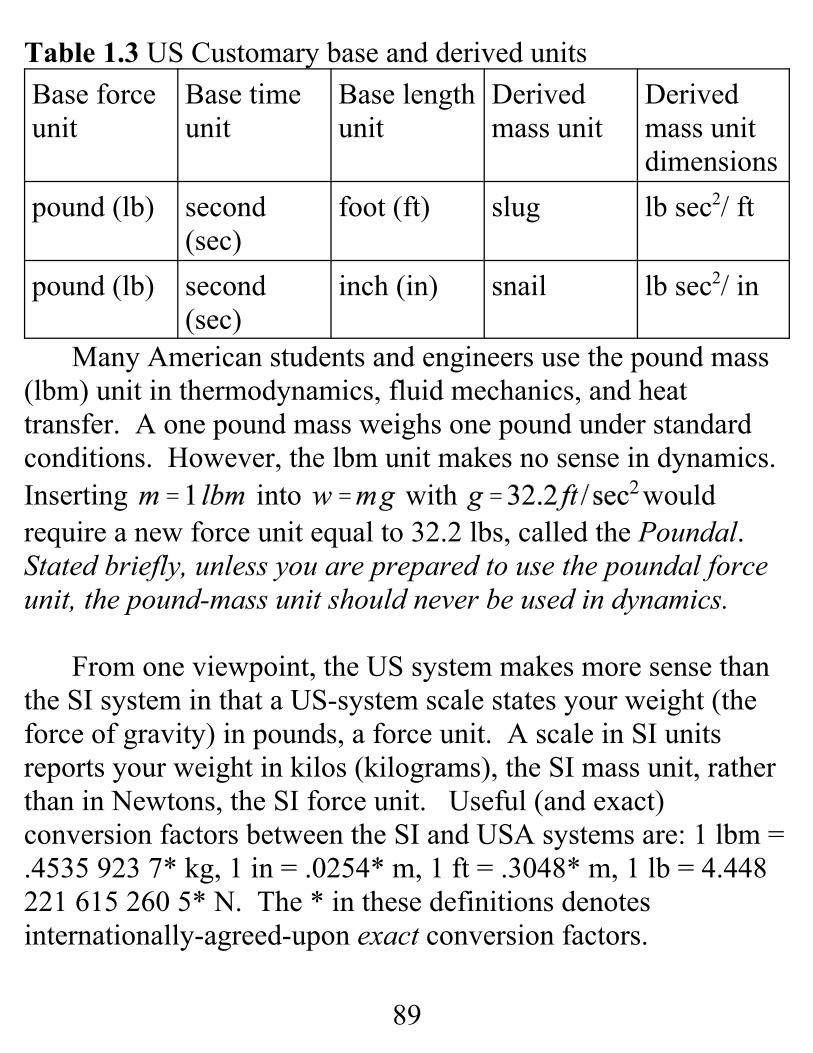
Table 1.3 US Customary base and derived unitsBase forceunit

Base timeunit

Base lengthunit

Derivedmass unit

Derivedmass unitdimensions

pound (lb) second(sec)

foot (ft) slug lb sec2/ ft

pound (lb) second(sec)

inch (in) snail lb sec2/ in

Many American students and engineers use the pound mass(lbm) unit in thermodynamics, fluid mechanics, and heattransfer. A one pound mass weighs one pound under standardconditions. However, the lbm unit makes no sense in dynamics.Inserting into with wouldrequire a new force unit equal to 32.2 lbs, called the Poundal.Stated briefly, unless you are prepared to use the poundal forceunit, the pound-mass unit should never be used in dynamics.

From one viewpoint, the US system makes more sense thanthe SI system in that a US-system scale states your weight (theforce of gravity) in pounds, a force unit. A scale in SI unitsreports your weight in kilos (kilograms), the SI mass unit, ratherthan in Newtons, the SI force unit. Useful (and exact)conversion factors between the SI and USA systems are: 1 lbm =.4535 923 7* kg, 1 in = .0254* m, 1 ft = .3048* m, 1 lb = 4.448221 615 260 5* N. The * in these definitions denotesinternationally-agreed-upon exact conversion factors.

90

Conversions between SI and US Customary unit systemsshould be checked carefully. An article in the 4 October 1999issue of Aviation Week and Space Technology states,” Engineershave discovered that use of English instead of metric units in anavigation software table contributed to, if not caused, the loss ofMars Climate Orbiter during orbit injection on Sept. 23.” Thispress report covers a highly visible and public failure; however,less spectacular mistakes are regularly made in unit conversions.

92

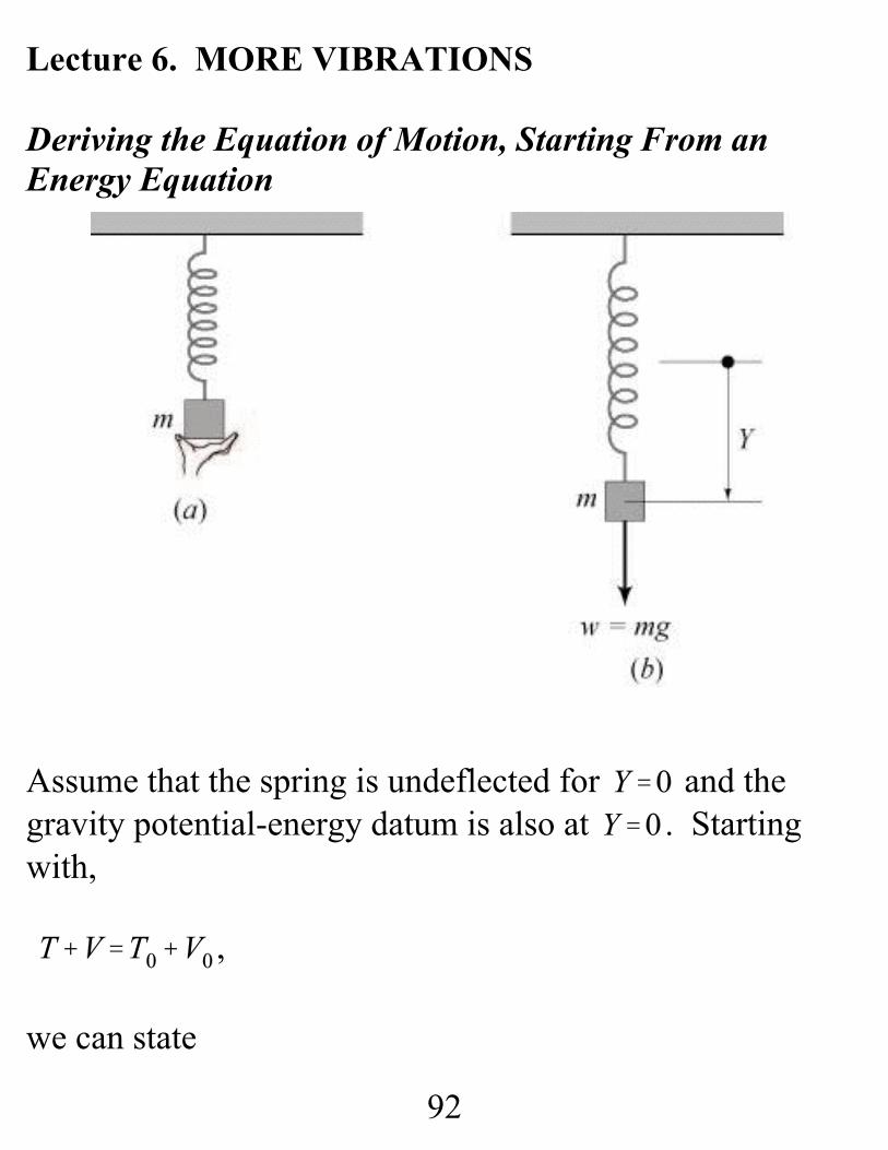
Lecture 6. MORE VIBRATIONS

Deriving the Equation of Motion, Starting From anEnergy Equation

Assume that the spring is undeflected for and thegravity potential-energy datum is also at . Startingwith,

,

we can state

93

The negative sign applies for the gravity potential energybecause Y is below the datum. Differentiating with respectto Y gives

In many cases, the differential equation of motion isobtained more easily from an energy equation than fromNewton’s 2nd law.

Equilibrium Conditions. Equilibrium for the particlegoverned by the mass-spring differential equation,

occurs for , and defines the equilibrium position

We looked at motion about the equilibrium position by

94

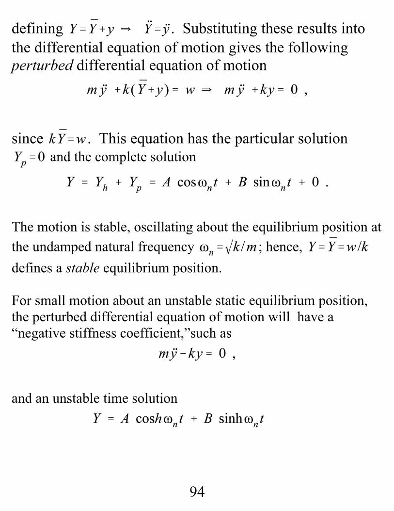
defining . Substituting these results intothe differential equation of motion gives the followingperturbed differential equation of motion

since . This equation has the particular solution and the complete solution

The motion is stable, oscillating about the equilibrium position atthe undamped natural frequency ; hence, defines a stable equilibrium position.

For small motion about an unstable static equilibrium position,the perturbed differential equation of motion will have a“negative stiffness coefficient,”such as

and an unstable time solution

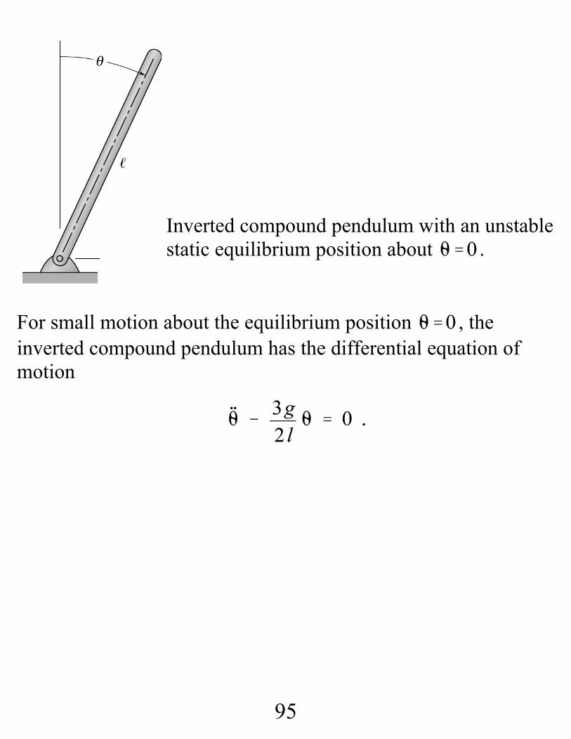
95

Inverted compound pendulum with an unstablestatic equilibrium position about .

For small motion about the equilibrium position , theinverted compound pendulum has the differential equation ofmotion

96

External time-varying force. Adding the external time-varyingforce to the harmonic oscillator (mass-spring)system yields the differential equation

The energy-integral substitution,

gives

and integration gives

This equation is a specific example of the general equation

97

An external time-varying force is a nonconservative force andproduces nonconservative work. The right-hand side integralcannot be evaluated unless the solution for the differentialequation is known.

Hence, for nonconservative forces that are functions of time,neither the energy-integral substitution nor the work-energyequation is useful in solving the differential equation of motion. The substitution is normally helpful in solving the differentialequation when the acceleration can be expressed as a function ofdisplacement only.

98

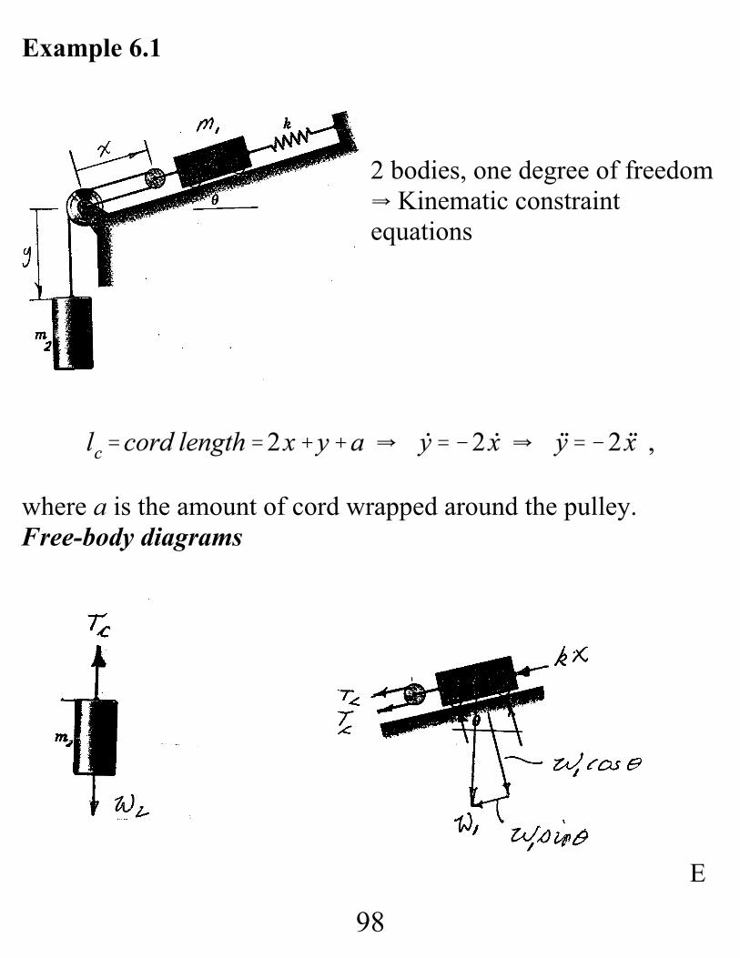
Example 6.1

2 bodies, one degree of freedomY Kinematic constraintequations

where a is the amount of cord wrapped around the pulley.Free-body diagrams

E

99

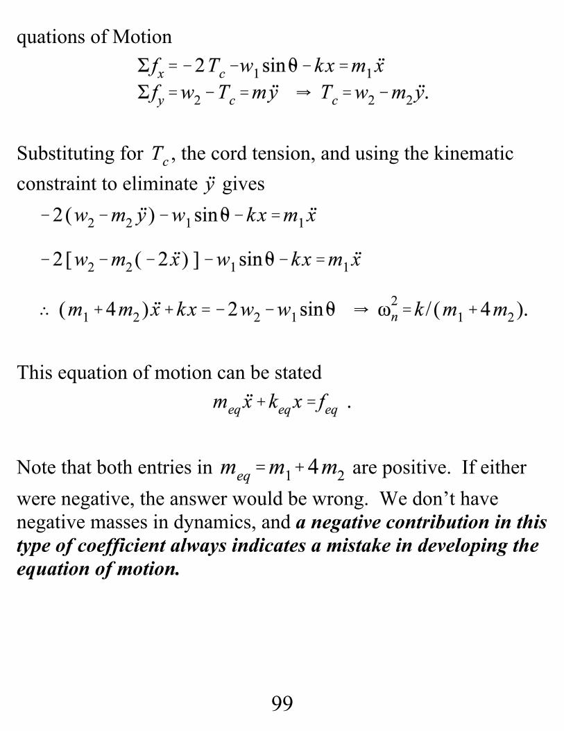
quations of Motion

Substituting for , the cord tension, and using the kinematicconstraint to eliminate gives

This equation of motion can be stated

Note that both entries in are positive. If eitherwere negative, the answer would be wrong. We don’t havenegative masses in dynamics, and a negative contribution in thistype of coefficient always indicates a mistake in developing theequation of motion.

100

Strategy for Deriving and Verifying the Equation of Motionfrom :1. Select Coordinates and draw them on your figure. Yourchoice for coordinates will establish the + and - signs fordisplacements, velocities, accelerations and forces. Check to seeif there is a relation between your coordinates. If there is arelationship, write out the corresponding kinematic constraintequation(s).

2. Draw free-body diagrams corresponding to positivedisplacements and velocities for your bodies. In the presentexample a positive x displacement produced a compression forcein the spring acting in the -x direction.

3. Use to state the equations of motion with + and -forces defined by the + and - signs of your coordinates.

4. Use the kinematic constraint equation(s) to eliminate excessvariables to produce an equation of motion.

5. If your equation has the form , check tosee that the individual contributions for and are positive.

Think about the degrees of freedom for your system. A onedegree-of-freedom (1DOF) system needs one coordinate to

101

define all of the bodies’ positions. A 2DOF system needs twocoordinate to define all of the bodies’ positions, etc. Example6.1 has two coordinates but only one degree of freedom.

Equation of Motion for motion about equilibrium

Equilibrium is defined by and implies

For motion about the equilibrium position defined by,

102

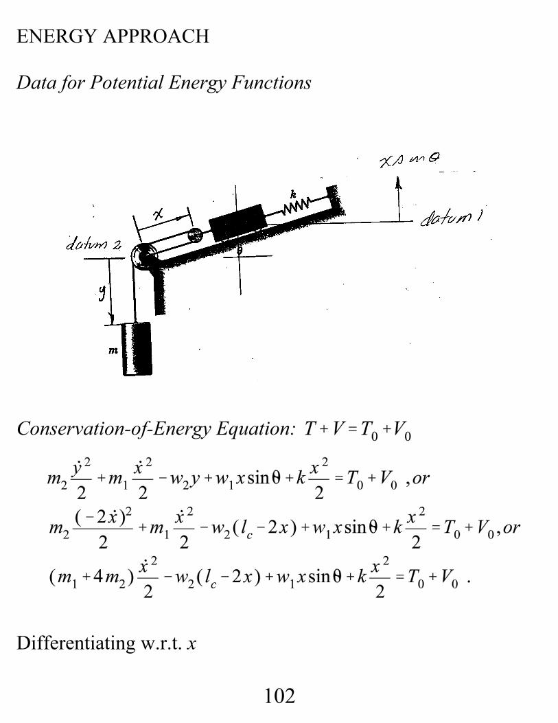
ENERGY APPROACH

Data for Potential Energy Functions

Conservation-of-Energy Equation:

Differentiating w.r.t. x

103

104

LECTURE 7. MORE VIBRATIONS

`

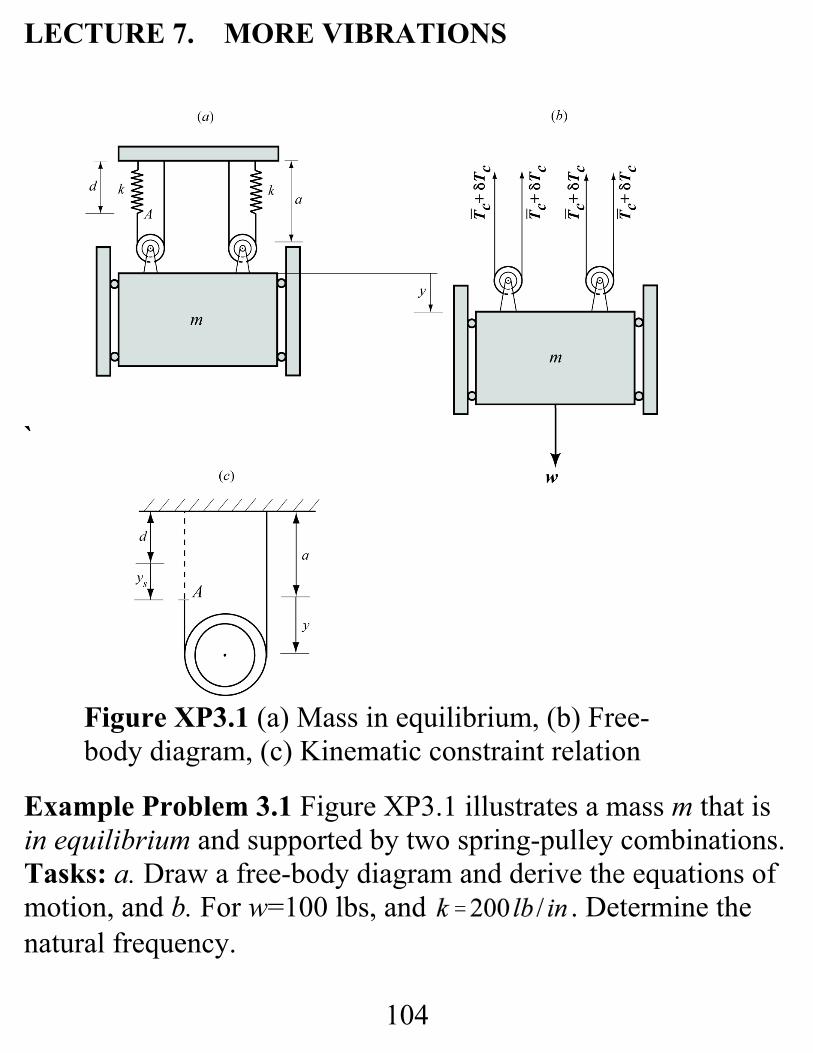
Example Problem 3.1 Figure XP3.1 illustrates a mass m that isin equilibrium and supported by two spring-pulley combinations. Tasks: a. Draw a free-body diagram and derive the equations ofmotion, and b. For w=100 lbs, and . Determine thenatural frequency.

Figure XP3.1 (a) Mass in equilibrium, (b) Free-body diagram, (c) Kinematic constraint relation

105

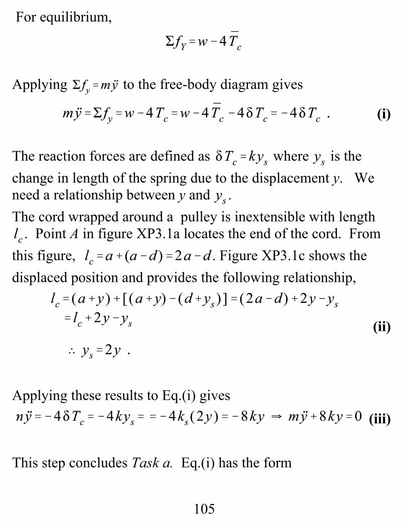
For equilibrium,

Applying to the free-body diagram gives

The reaction forces are defined as where is thechange in length of the spring due to the displacement y. Weneed a relationship between y and . The cord wrapped around a pulley is inextensible with length

. Point A in figure XP3.1a locates the end of the cord. Fromthis figure, . Figure XP3.1c shows thedisplaced position and provides the following relationship,

Applying these results to Eq.(i) gives

This step concludes Task a. Eq.(i) has the form

(i)

(ii)

(iii)

106

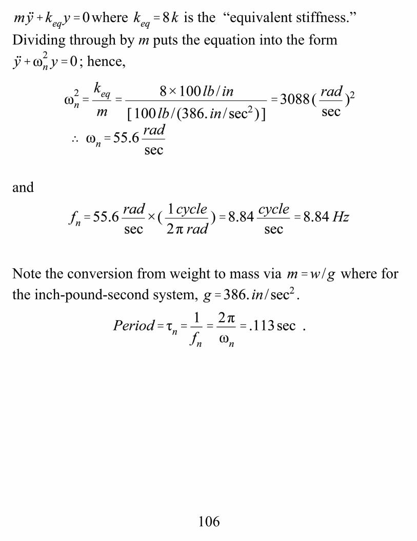
where is the “equivalent stiffness.” Dividing through by m puts the equation into the form

; hence,

and

Note the conversion from weight to mass via where forthe inch-pound-second system, .

107

Deriving Equation of Motion From Conservation of Energy

Differentiating w.r.t. y gives

The Simple Pendulum, Linearization of nonlinearDifferential Equations for smallmotion about an equilibrium

108

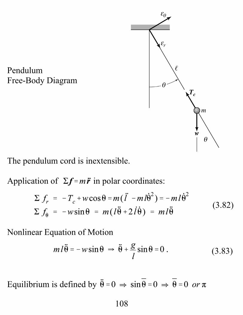
(3.82)

(3.83)

Pendulum Free-Body Diagram

The pendulum cord is inextensible.

Application of in polar coordinates:

Nonlinear Equation of Motion

Equilibrium is defined by

109

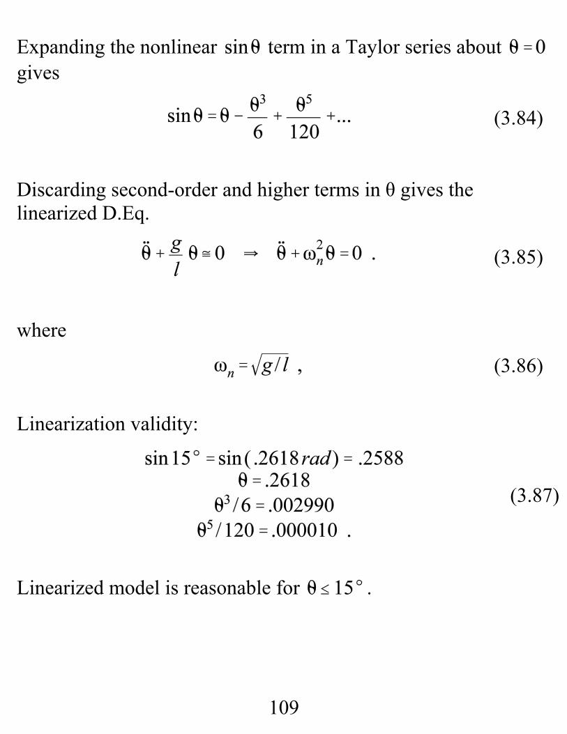
(3.84)

(3.85)

(3.87)

(3.86)

Expanding the nonlinear term in a Taylor series about gives

Discarding second-order and higher terms in θ gives thelinearized D.Eq.

where

Linearization validity:

Linearized model is reasonable for .

110

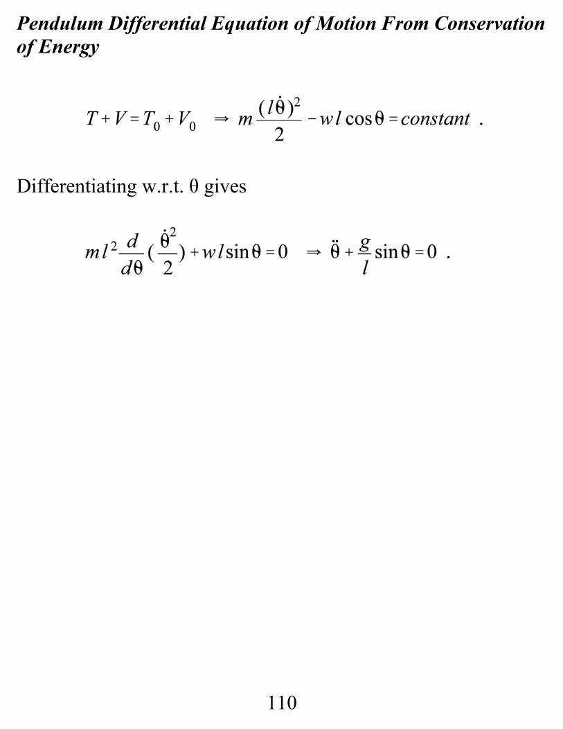
Pendulum Differential Equation of Motion From Conservationof Energy

Differentiating w.r.t. θ gives

111

ENERGY DISSIPATION—Viscous Damping

Automatic door-closers and shock absorbers for automobilesprovide common examples of energy dissipation that isdeliberately introduced into mechanical systems to limit peakresponse of motion.

As illustrated above, a thin layer of fluid lies between the pistonand cylinder. As the piston is moved, shear flow is produced inthe fluid which develops a resistance force that is proportional tothe velocity of the piston relative to the cylinder. The flowbetween the piston and the cylinder is laminar, versus turbulentflow which occurs commonly in pipe flow and will be covered inyour fluid mechanics course. The piston free-body diagramshows a reaction force that is proportional to the piston’s velocity and acting in a direction that is opposite to the piston’s velocity

112

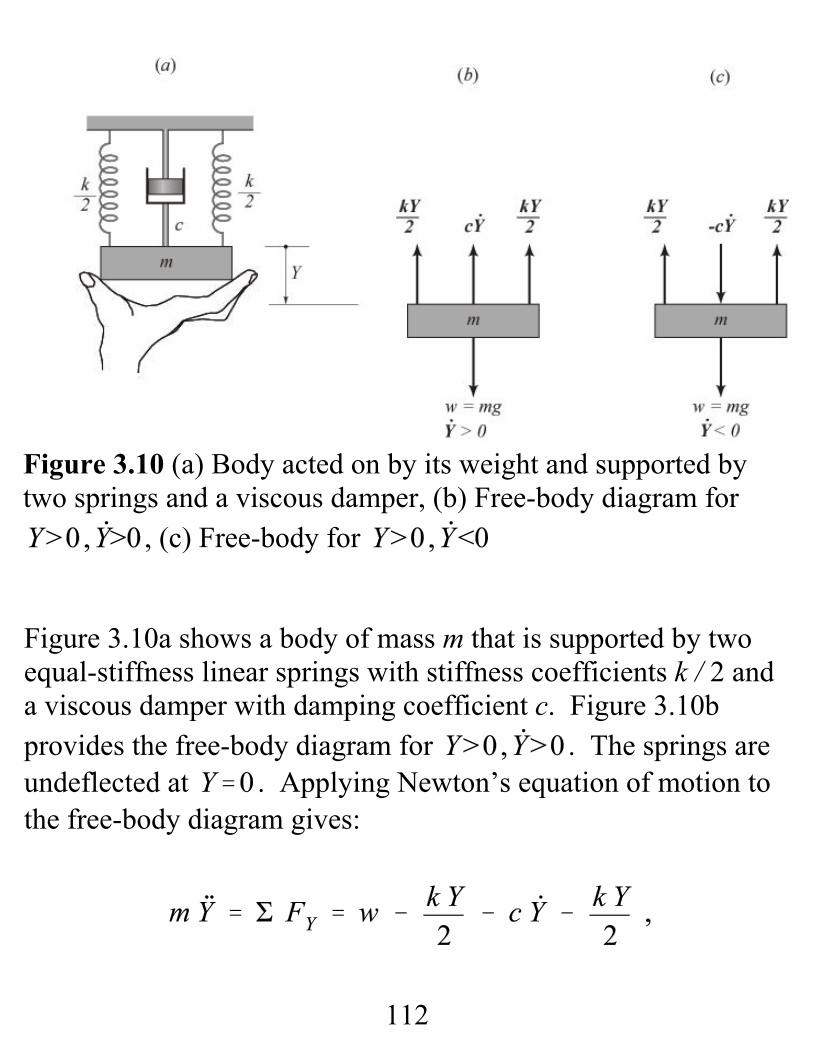
Figure 3.10a shows a body of mass m that is supported by twoequal-stiffness linear springs with stiffness coefficients k / 2 anda viscous damper with damping coefficient c. Figure 3.10bprovides the free-body diagram for . The springs areundeflected at . Applying Newton’s equation of motion tothe free-body diagram gives:

Figure 3.10 (a) Body acted on by its weight and supported bytwo springs and a viscous damper, (b) Free-body diagram for

, (c) Free-body for

113

(3.21)

(3.22)

or

Dividing through by m gives

where

ζ is called the linear damping factor.

Transient Solution due to Initial Conditions and Weight.

Homogeneous differential Equation

Assumed solution: Yh=Aest yields:

114

(3.23)

(3.24)

(3.25)

Since A … 0, and

This is the characteristic equation. For , the mass iscritically damped and does not oscillate. For ζ<1, the roots are

is called the damped natural frequency. The tworoots defined by Eq.(3.24) are

The homogeneous solution looks like

where A1 and A2 are complex coefficients. Substituting theidentities

into Eq.(3.25) yields a final homogeneous solution of the form

115

(3.26)

(3.27)

where A and B are real constants. The complete solution is

For I.C.’s , starting with Eq.(3.27) yields

To evaluate B, we differentiate Eq.(3.27), obtaining

Evaluating this expression at t = 0 gives

Hence,

116

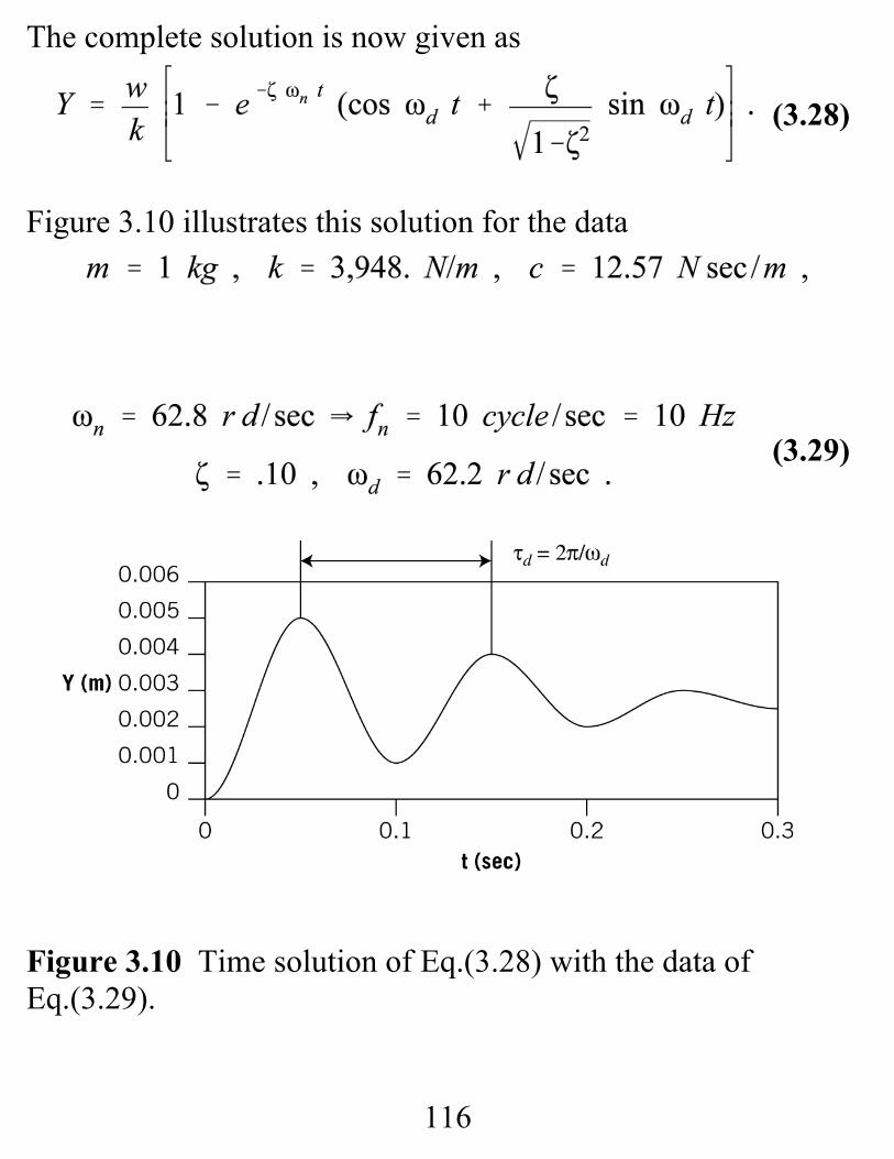
(3.28)

(3.29)

The complete solution is now given as

Figure 3.10 illustrates this solution for the data

Figure 3.10 Time solution of Eq.(3.28) with the data ofEq.(3.29).

117

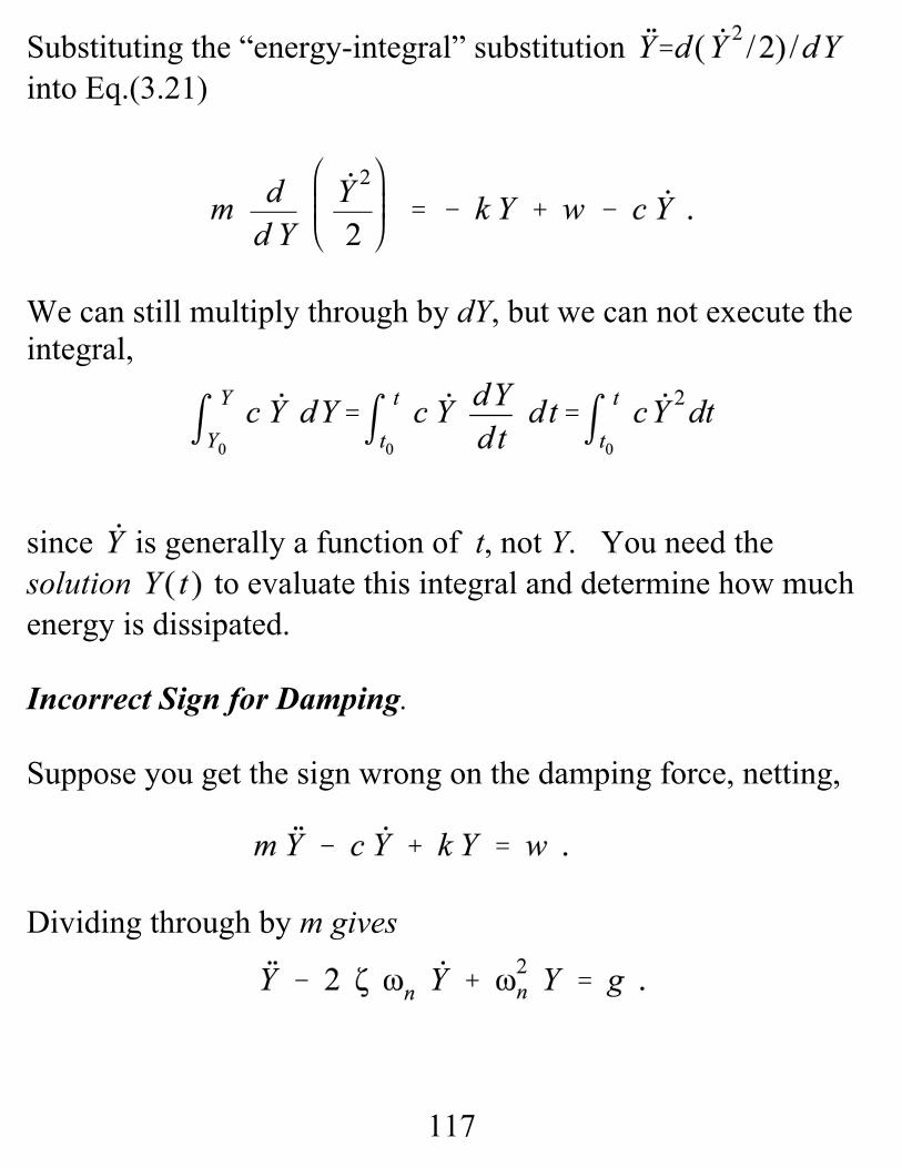
Substituting the “energy-integral” substitution into Eq.(3.21)

We can still multiply through by dY, but we can not execute theintegral,

since is generally a function of t, not Y. You need thesolution to evaluate this integral and determine how muchenergy is dissipated.

Incorrect Sign for Damping.

Suppose you get the sign wrong on the damping force, netting,

Dividing through by m gives

118

the general solution is now

Instead of decaying exponentially with time, the solution growsexponentially with time.

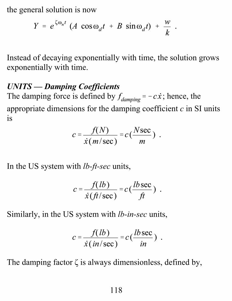
UNITS — Damping CoefficientsThe damping force is defined by ; hence, theappropriate dimensions for the damping coefficient c in SI unitsis

In the US system with lb-ft-sec units,

Similarly, in the US system with lb-in-sec units,

The damping factor ζ is always dimensionless, defined by,

119

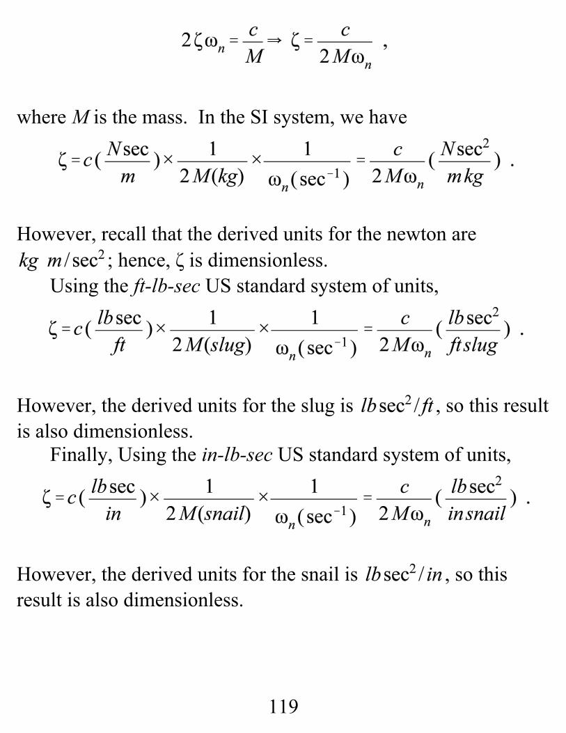
where M is the mass. In the SI system, we have

However, recall that the derived units for the newton are; hence, ζ is dimensionless.

Using the ft-lb-sec US standard system of units,

However, the derived units for the slug is , so this resultis also dimensionless.

Finally, Using the in-lb-sec US standard system of units,

However, the derived units for the snail is , so thisresult is also dimensionless.

120

(3.30)

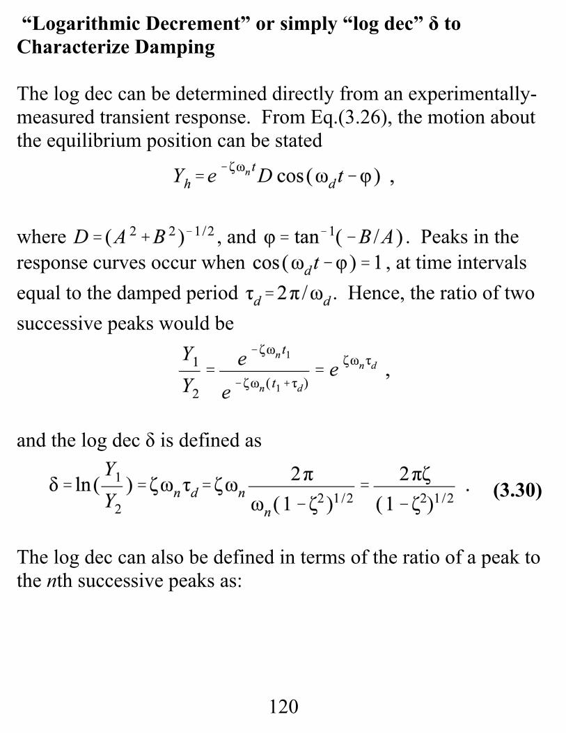
“Logarithmic Decrement” or simply “log dec” δ toCharacterize Damping

The log dec can be determined directly from an experimentally-measured transient response. From Eq.(3.26), the motion aboutthe equilibrium position can be stated

where , and . Peaks in theresponse curves occur when , at time intervalsequal to the damped period . Hence, the ratio of twosuccessive peaks would be

and the log dec δ is defined as

The log dec can also be defined in terms of the ratio of a peak tothe nth successive peaks as:

121

(3.31)

(3.31)

Note in Eq.(3.30) that δ becomes unbounded as . In manydynamic systems, the damping factor is small, , and

.

In stability calculations for systems with unstable eigenvalues,negative log dec’s are regularly stated.

Solving for the damping factor ζ in terms of δ from Eq.(3.30)gives

The effect of damping in the model can becharacterized in terms of the damping factor ζ and the log-dec δ.

122

(3.31)

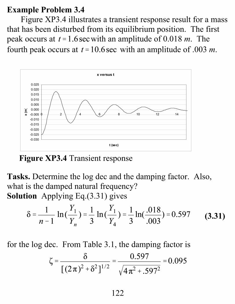
Example Problem 3.4Figure XP3.4 illustrates a transient response result for a mass

that has been disturbed from its equilibrium position. The firstpeak occurs at with an amplitude of 0.018 m. Thefourth peak occurs at with an amplitude of .003 m.

Tasks. Determine the log dec and the damping factor. Also,what is the damped natural frequency?Solution Applying Eq.(3.31) gives

for the log dec. From Table 3.1, the damping factor is

x versus t

-0.030-0.025-0.020-0.015-0.010-0.0050.0000.0050.0100.0150.0200.025

0 2 4 6 8 10 12 14

t (sec)

x (m

)

Figure XP3.4 Transient response

123

The damped period for the system is obtained as. Hence,

.

Percent of Critical DampingRecall that Y critical damping A “percent of criticaldamping” is also used to specify the amount of availabledamping. For example, implies 10% of critical damping.

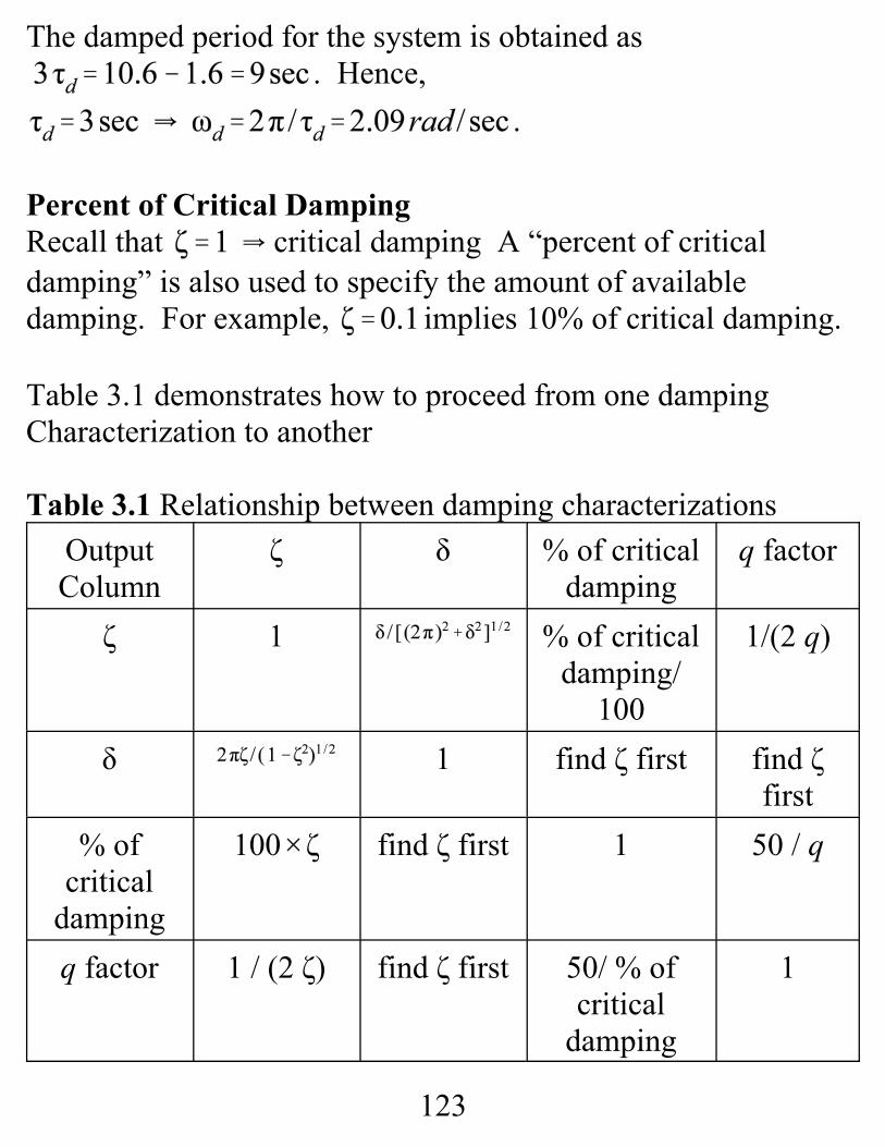
Table 3.1 demonstrates how to proceed from one dampingCharacterization to another

Table 3.1 Relationship between damping characterizationsOutputColumn

ζ δ % of criticaldamping

q factor

ζ 1 % of criticaldamping/

100

1/(2 q)

δ 1 find ζ first find ζfirst

% ofcritical

damping

100 ζ find ζ first 1 50 / q

q factor 1 / (2 ζ) find ζ first 50/ % ofcritical

damping

1

124

Important Concept and Knowledge Questions

How is the reaction force due to viscous damping defined?

In the differential equation of motion for a damped, spring-mass system, what is the correct sign for c , the lineardamping coefficient?

What is implied by a negative damping coefficient c?

What are c’s dimensions in the inch-pound-second, foot-pound-second, newton-kilogram-second, newton-millimeter-second systems?

What is the damped natural frequency?

What is the damping factor ζ ?

How is the critical damping factor defined, and what doescritical damping imply about free motion?

What is the log dec?

125

(B.1)

(B.2)

Lecture 8. TRANSIENT SOLUTIONS 1, FORCEDRESPONSE AND INITIAL CONDITIONS

IntroductionDifferential equations in dynamics normally arise from

Newton’s second law of motion, Accordingly, indynamics, systems of coupled second order differential equationsare the norm. Occasionally, the equation of motion for a particleor rigid body has the form, , and the energy-integral substitution,

reduces the second-order equation, with time t as the independentvariable, to the first-order differential equation,

with displacement y as the independent variable and as thedependent variable. Systems of first order equations arise in heattransfer, RC circuits, population studies, etc.

126

(B.8)

Undamped Spring-Mass ModelThe undamped spring-mass system with weight acting as aforcing function can be stated

The homogeneous differential equation is obtained by setting theright-hand side to zero, netting in this case . Insolving any linear second-order differential equation, we use thefollowing steps:

(i). Solve the homogeneous equation for , which willinclude two arbitrary constants A and B,

(ii). Solve for the particular solution that satisfies theright-hand side of the equation,

(iii). Form the complete solution , and

(iv). Use the complete solution to solve for the two unknownconstants A and B that satisfy the problem’s initial conditions.

127

(B.9)

The formal solution to the homogeneous differentialequation, , is obtained by assuming a solution of the

form . We have previously developedthe homogeneous solution as

where .Any constant-coefficient linear ordinary differential equation

can be solved by Laplace transforms including the particularsolution. However, most particular solutions can be obtained byan inspection of the right-hand side terms and the differentialequation itself. For Eq.(B.8), the right hand side is constant, anda guessed constant solution of the form yields

where is the static deflection due to the weight w. Notethat this particular solution is linearly proportional to theexcitation on the right-hand side of Eq.(B.8).

128

(B.10)

(B.11)

The complete solution to is

Assuming that the initial conditions are , ,we can first solve for the constant A via

Similarly, , nets

and the complete solution (satisfying the specified initialconditions) is

Suppose the spring-mass system is acted on by an externalforce that increases linearly with time, netting the differentialequation of motion,

129

( B.12)

(B.13)

This equation has the same homogeneous differential equationand solution; however, a new particular solution is required. Byinspection, a solution of the form will work. Substituting this guessed solution into Eq.(B.12)produces

Eq.(B.12)’s complete solution is now

130

Table B.1 provides three particular solutions.

Table B.1. Particular solutions for .

Excitation,

a t

131

(B.18)

(B.19)

Consider the following version of Eq.(B.8)

Since this equation is linear, from Table B.1 and thehomogeneous solution defined by Eq.(B.9), from superposition,the complete solution is

Spring-Mass-Damper ModelThe equation of motion for a spring-mass-damper system actedupon by weight can be stated

The homogeneous solution is obtained (again) by assuming asolution of the form . Substituting into the homogeneous differential equation nets

This result holds, since neither A nor is zero.

132

(B.21)

(B.20)

The following three solution possibilities exist for Eq.(B.19):

(i). , critically damped motion,

(ii). , over-damped motion, and

(iii). , under-damped motion.

For , the roots to the characteristic Eq.(B.19) are

Note that two real, negative roots are obtained, netting thehomogeneous solution,

where are real constants. The overdamped solution is thesum of two exponentially decaying terms.

For (critical damping), the characteristic Eq.(B.19)produces the single root , and single solution,

. This homogeneous solution (containing only oneconstant) is not adequate to satisfy two initial conditions

133

(B.25)

(B.26)

(B.22)

(position and velocity). For less than obvious reasons, thecomplete homogeneous solution is

where are real constants. The second term in this solution also satisfies the differential equation as can be confirmed bysubstituting for . The critically-damped solution is interestingfrom a mathematical viewpoint as a limiting condition, but hasminimal direct engineering value.

For , the homogeneous equation, hasthe solution form

where are real constants, and .

The particular solution for is

, and the complete solution is

134

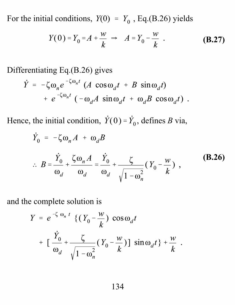
(B.27)

(B.26)

For the initial conditions, , Eq.(B.26) yields

Differentiating Eq.(B.26) gives

Hence, the initial condition, , defines B via,

and the complete solution is

135

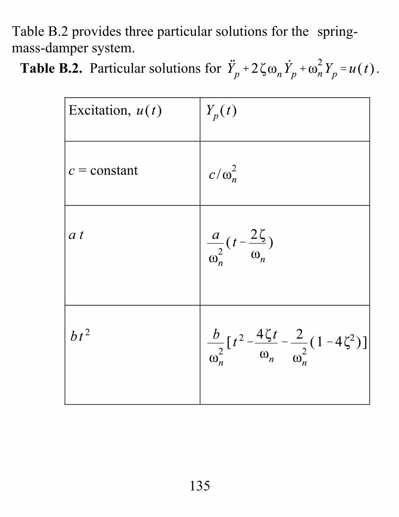
Table B.2 provides three particular solutions for the spring-mass-damper system.

Table B.2. Particular solutions for .

Excitation,

c = constant

a t

136

As with the undamped equation, the following basic steps aretaken to produce a complete solution for :

a. The homogeneous solution,, is developed for

and involves the two constants A andB.

b. The particular solution is developed to satisfy the

right hand side of the equation .

c. The complete solution, , is formed,and the arbitrary constants A and B are determined from thecomplete solution such that the complete solution satisfiesthe initial conditions.

137

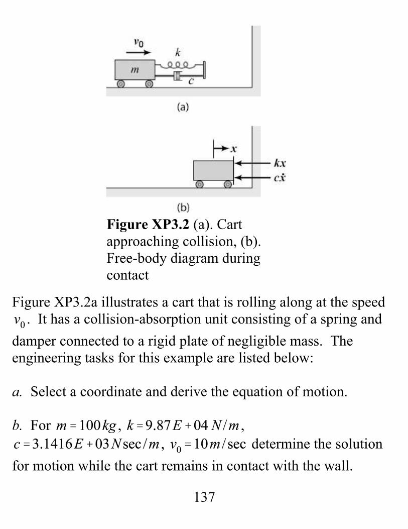
Figure XP3.2 (a). Cartapproaching collision, (b).Free-body diagram duringcontact

Figure XP3.2a illustrates a cart that is rolling along at the speed. It has a collision-absorption unit consisting of a spring and

damper connected to a rigid plate of negligible mass. Theengineering tasks for this example are listed below:

a. Select a coordinate and derive the equation of motion.

b. For , ,, determine the solution

for motion while the cart remains in contact with the wall.

138

(i)

(ii)

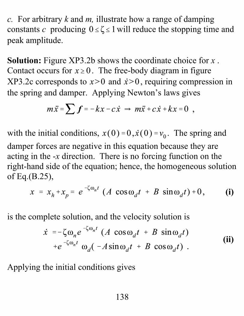
c. For arbitrary k and m, illustrate how a range of dampingconstants c producing will reduce the stopping time andpeak amplitude.

Solution: Figure XP3.2b shows the coordinate choice for x . Contact occurs for . The free-body diagram in figureXP3.2c corresponds to and , requiring compression inthe spring and damper. Applying Newton’s laws gives

with the initial conditions, . The spring anddamper forces are negative in this equation because they areacting in the -x direction. There is no forcing function on theright-hand side of the equation; hence, the homogeneous solutionof Eq.(B.25),

is the complete solution, and the velocity solution is

Applying the initial conditions gives

1

The equation has an infinite number of solutionsdefined by:

139

(iii)

Substituting back into (i) and (ii) gives

where .

The cart loses contact with the wall when . Tf isdefined from the first of Eqs.(iii) by 1.The problem parameters net

140

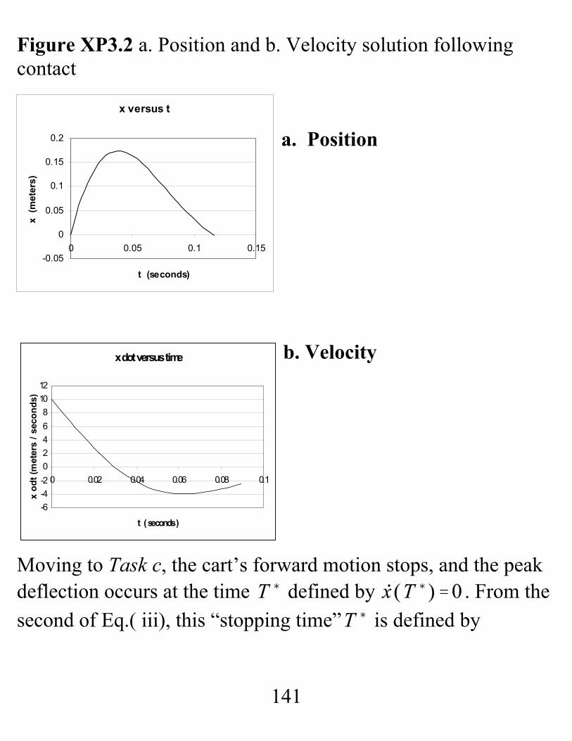
Plots for x and x(t) are provided below for .

141

x versus t

-0.05

0

0.05

0.1

0.15

0.2

0 0.05 0.1 0.15

t (seconds)

x (m

eter

s)

x dot versus time

-6-4-2024681012

0 0.02 0.04 0.06 0.08 0.1

t ( seconds )

x od

t (m

eter

s / s

econ

ds)

Figure XP3.2 a. Position and b. Velocity solution followingcontact

a. Position

b. Velocity

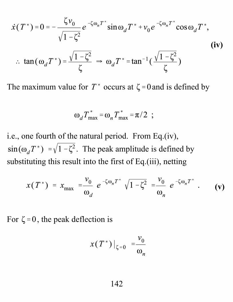
Moving to Task c, the cart’s forward motion stops, and the peakdeflection occurs at the time defined by . From thesecond of Eq.( iii), this “stopping time” is defined by

142

(v)

(iv)

The maximum value for occurs at and is defined by

i.e., one fourth of the natural period. From Eq.(iv),. The peak amplitude is defined by

substituting this result into the first of Eq.(iii), netting

For , the peak deflection is

143

Reduction in stopping time

0

0.2

0.4

0.6

0.8

1

1.2

0 0.2 0.4 0.6 0.8 1 1.2

zeta

T* /

(T* @

zet

a =

0)

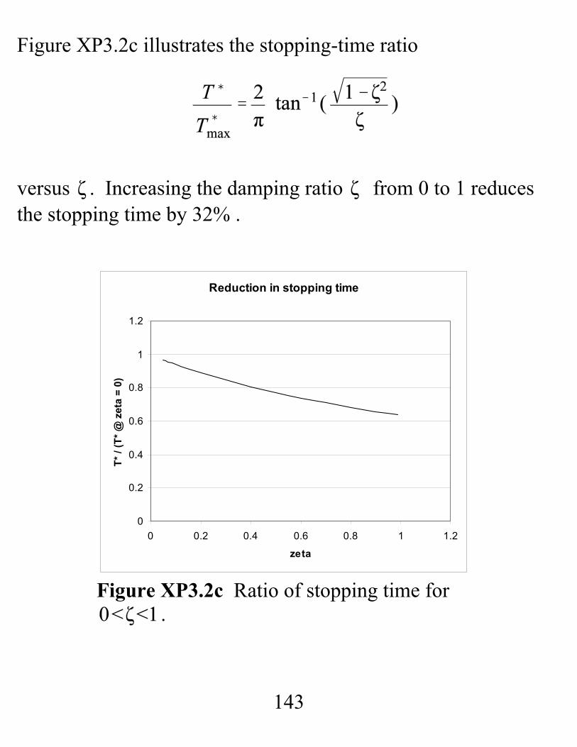
Figure XP3.2c Ratio of stopping time for.

Figure XP3.2c illustrates the stopping-time ratio

versus . Increasing the damping ratio from 0 to 1 reducesthe stopping time by 32% .

144

Relative Reduction in Peak Amplitudes

0

0.1

0.2

0.3

0.4

0.5

0.6

0.7

0.8

0.9

1

0 0.2 0.4 0.6 0.8 1 1.2

zeta

X(T*

)/ X(

T* @

zeta

= 0

)

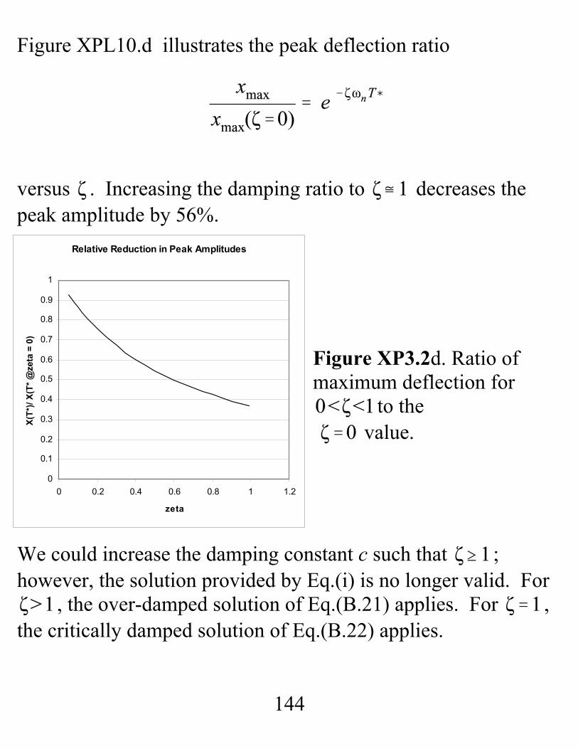
Figure XPL10.d illustrates the peak deflection ratio

versus . Increasing the damping ratio to decreases thepeak amplitude by 56%.

Figure XP3.2d. Ratio ofmaximum deflection for

to the value.

We could increase the damping constant c such that ;however, the solution provided by Eq.(i) is no longer valid. For

, the over-damped solution of Eq.(B.21) applies. For ,the critically damped solution of Eq.(B.22) applies.

145

Lecture 9. More Transient Solutions, Base Excitation

Example Problem L9.1 Consider the model with initial conditions

. The parameters k, m, and c are defined by , , and . These

data produce:

The force is defined by the half-sine wave pulse illustratedbelow, and defined by

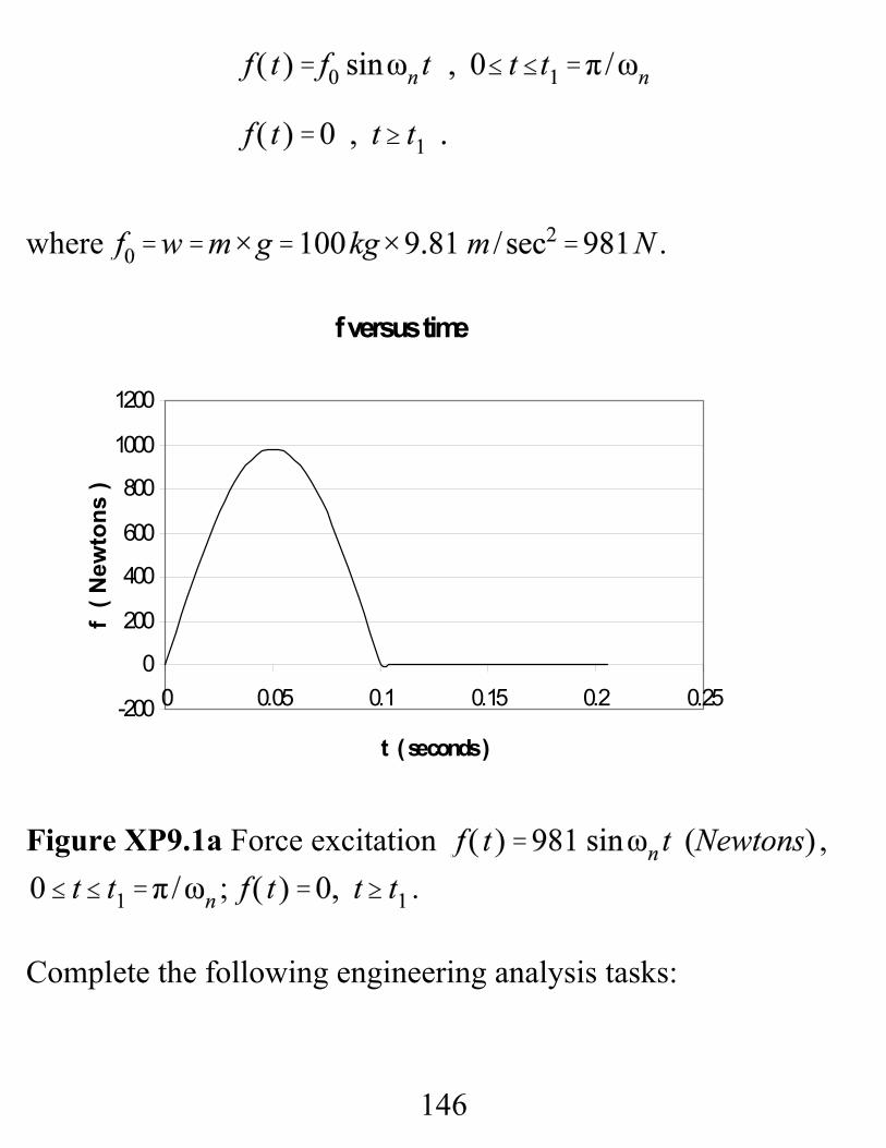
146

f versus time

-200

0

200

400

600

800

1000

1200

0 0.05 0.1 0.15 0.2 0.25

t ( seconds )

f ( N

ewto

ns )

where .

Figure XP9.1a Force excitation , ; .

Complete the following engineering analysis tasks:

147

a. Determine the solution for .

b. Determine the solution for .

c. Plot the solution for

Solution. In lecture 11, we will develop the particular solutionfor as , where

For , , ,and the particular solution is

The complete solution is

148

A is solved via

To determine B, we start with

Evaluating,

The complete solution satisfying the initial conditions is

149

Y dot versus time

-5.00E-02

0.00E+00

5.00E-02

1.00E-01

1.50E-01

2.00E-01

2.50E-01

3.00E-01

0 0.02 0.04 0.06 0.08 0.1 0.12

t ( seconds )

Y do

t ( m

eter

s / s

econ

ds )

Y versus t

0.00E+002.00E-034.00E-036.00E-038.00E-031.00E-021.20E-021.40E-021.60E-02

0 0.02 0.04 0.06 0.08 0.1 0.12

t ( seconds )

Y (

met

ers

)

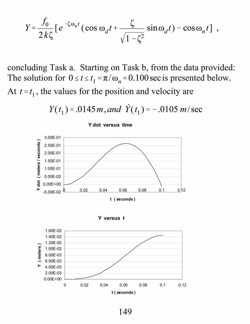
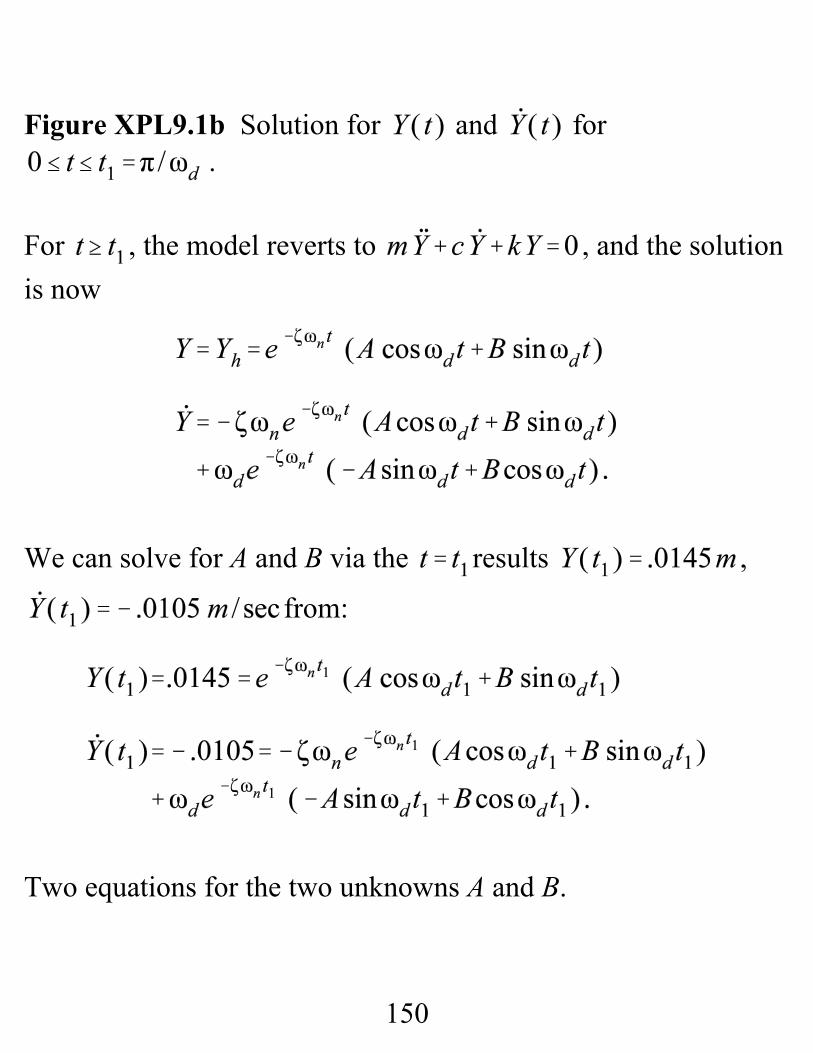
concluding Task a. Starting on Task b, from the data provided:The solution for is presented below. At , the values for the position and velocity are

150

Figure XPL9.1b Solution for and for .

For , the model reverts to , and the solutionis now

We can solve for A and B via the results ,

from:

Two equations for the two unknowns A and B.

151

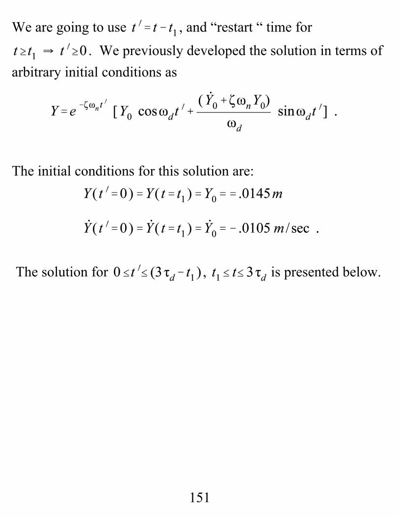
We are going to use , and “restart “ time for. We previously developed the solution in terms of

arbitrary initial conditions as

The initial conditions for this solution are:

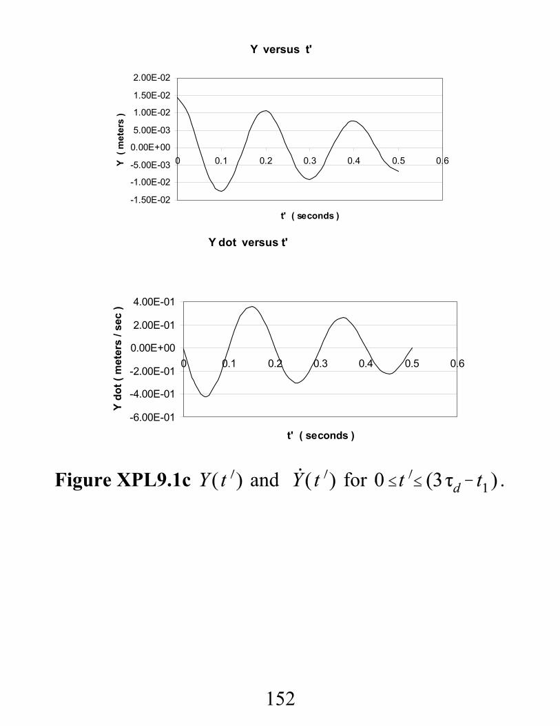
The solution for , is presented below.

152

Y versus t'

-1.50E-02

-1.00E-02

-5.00E-03

0.00E+00

5.00E-03

1.00E-02

1.50E-02

2.00E-02

0 0.1 0.2 0.3 0.4 0.5 0.6

t' ( seconds )

Y (

met

ers

)

Y dot versus t'

-6.00E-01

-4.00E-01

-2.00E-01

0.00E+00

2.00E-01

4.00E-01

0 0.1 0.2 0.3 0.4 0.5 0.6

t' ( seconds )

Y do

t ( m

eter

s / s

ec )

Figure XPL9.1c and for .

153

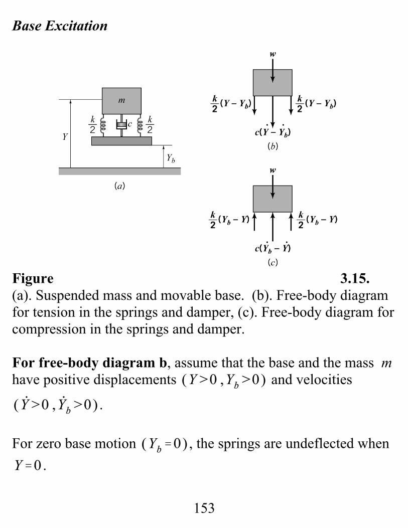
Base Excitation

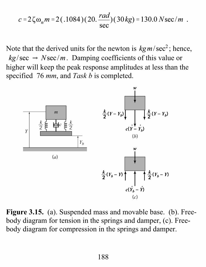
Figure 3.15. (a). Suspended mass and movable base. (b). Free-body diagramfor tension in the springs and damper, (c). Free-body diagram forcompression in the springs and damper.

For free-body diagram b, assume that the base and the mass mhave positive displacements and velocities

.

For zero base motion , the springs are undeflected when.

154

Assuming that the m’s displacement is greater than the basedisplacement means that the springs are in tension, and

the spring forces are defined by .

Assuming that the m’s velocity is greater than the base velocity, the damper is also in tension, and the damping force is

defined by .

Applying to the free-body diagram of figure 3.15b givesthe differential equation of motion

For free-body diagram c , the base displacement is greater thanthe mass displacement . With this assumed relativemotion, the springs are in compression, and the spring forces aredefined by . Similarly, assuming that the base

velocity is greater than m’s causes the damper to alsobe in compression, and the damper force is defined by

. The free-body diagram of figure 3.15C is

155

consistent with this assumed motion and leads to the differentialequation of motion

The short lesson from these developments is that the samegoverning equation should result for any assumed motion, sincethe governing equation applies for any position and velocity. Note that the following procedural steps were taken in arriving atthe equation of motion:

a. The nature of the motion was assumed e.g., ,

b. The spring or damper force was stated in a manner thatwas consistent with the assumed motion, e.g.,

,

c. The free-body diagram was drawn in a manner that wasconsistent with the assumed motion and its resultant springand damper forces., i.e., in tension or compression, and

d. Newton’s second law of motion was applied tothe free-body diagram to obtain the equation of motion.

Note: We have looked at only one arrangement for base

156

excitation. Your homework has several examples for which thesame procedure works, but the final equations are different.

156

Figure XP3.3 (a). Spring-mass-damper system with an appliedforce, (b). Applied force definition

Lecture 10. Transient Solutions 3 — More base ExcitationExample Problem XP3.3.

Figure XP3.3a illustrates a spring-mass-damper systemcharacterized by the following parameters: ,

, , with the forcingfunction illustrated. The mass system start from rest with thespring undeflected. The force increases linearly until

when it reaches a magnitude equal to . For , .Tasks: Determine the mass’s position and velocity at

. Plot for and .

Solution. This Example problem has the same stiffness and mass

157

(ii)

(i)

as Example problem 9.1; hence,

The equation of motion for is

For , the equation of motion is We will use the solution for the first equation for todetermine and , which we will then use as initialconditions in stating the solution to the second equation ofmotion for .

The applicable homogeneous solution is

From Table B.2, the particular solution for , is

158

(iii)

(iv)

Hence, the particular solution for is

and the complete solution is

The velocity is

Solving for the constants from the initial conditions gives

The complete solution satisfying the initial conditions is

159

(v)

Y versus t

0

0.002

0.004

0.006

0.008

0 0.05 0.1 0.15

t (seconds)

Y (m

eter

s)

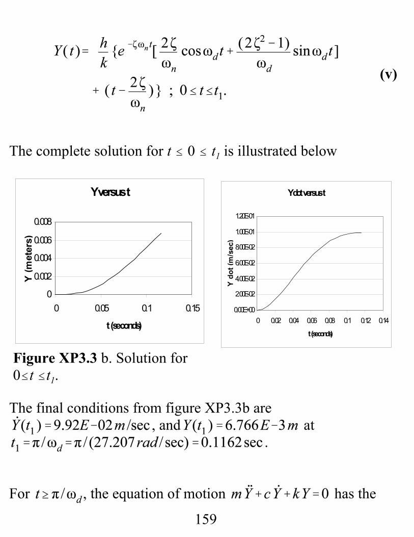
Figure XP3.3 b. Solution for0#t #t1.

Y dot versus t

0.00E+00

2.00E-02

4.00E-02

6.00E-02

8.00E-02

1.00E-01

1.20E-01

0 0.02 0.04 0.06 0.08 0.1 0.12 0.14

t (seconds)

Y do

t (m

/sec

)

The complete solution for t # 0 # t1 is illustrated below

The final conditions from figure XP3.3b are, and at

.

For , the equation of motion has the

160

solution

and derivative

We could solve for the unknown constants A and B via and . We are going

to take an easier tack by restarting time via the definition. Since,

the equation of motion is unchanged. The solution in terms of is

with the derivative

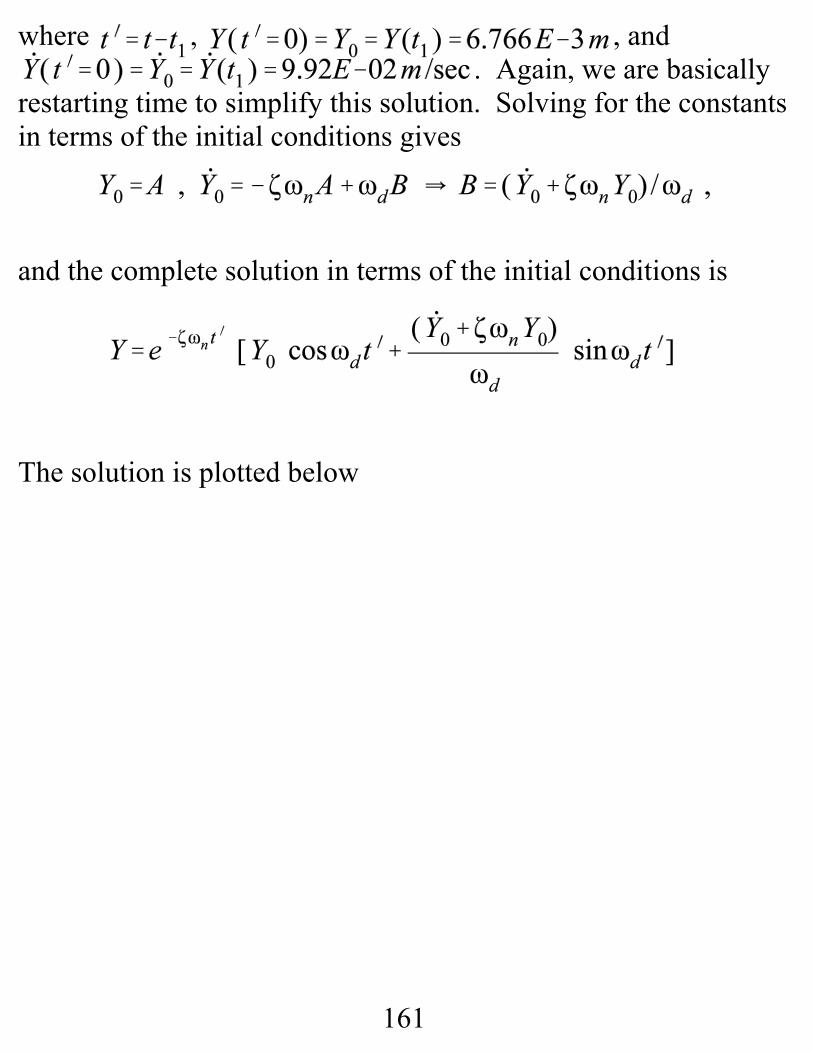
161

where , , and . Again, we are basically

restarting time to simplify this solution. Solving for the constantsin terms of the initial conditions gives

and the complete solution in terms of the initial conditions is

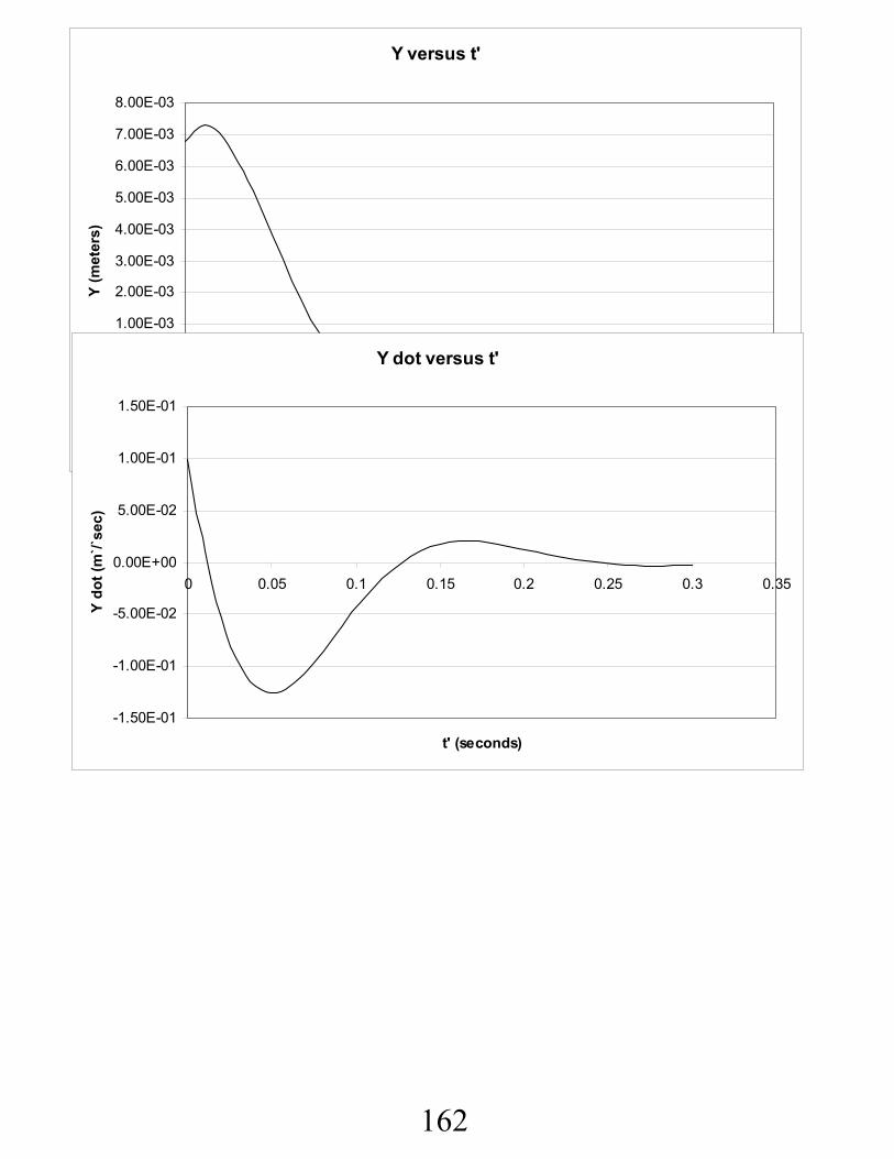
The solution is plotted below

162

Y versus t'

-2.00E-03

-1.00E-03

0.00E+00

1.00E-03

2.00E-03

3.00E-03

4.00E-03

5.00E-03

6.00E-03

7.00E-03

8.00E-03

0 0.05 0.1 0.15 0.2 0.25 0.3 0.35

t' (seconds)

Y (m

eter

s)

Y dot versus t'

-1.50E-01

-1.00E-01

-5.00E-02

0.00E+00

5.00E-02

1.00E-01

1.50E-01

0 0.05 0.1 0.15 0.2 0.25 0.3 0.35

t' (seconds)

Y do

t (m

`/`se

c)

163

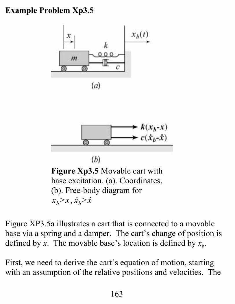
Example Problem Xp3.5

Figure XP3.5a illustrates a cart that is connected to a movablebase via a spring and a damper. The cart’s change of position isdefined by x. The movable base’s location is defined by xb.

First, we need to derive the cart’s equation of motion, startingwith an assumption of the relative positions and velocities. The

Figure Xp3.5 Movable cart withbase excitation. (a). Coordinates,(b). Free-body diagram for

164

(i)

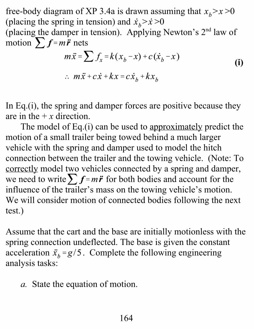
free-body diagram of XP 3.4a is drawn assuming that (placing the spring in tension) and (placing the damper in tension). Applying Newton’s 2nd law of motion nets

In Eq.(i), the spring and damper forces are positive because theyare in the + x direction.

The model of Eq.(i) can be used to approximately predict themotion of a small trailer being towed behind a much largervehicle with the spring and damper used to model the hitchconnection between the trailer and the towing vehicle. (Note: Tocorrectly model two vehicles connected by a spring and damper,we need to write for both bodies and account for theinfluence of the trailer’s mass on the towing vehicle’s motion. We will consider motion of connected bodies following the nexttest.)

Assume that the cart and the base are initially motionless with thespring connection undeflected. The base is given the constantacceleration . Complete the following engineeringanalysis tasks:

a. State the equation of motion.

165

b. State the homogeneous and particular solutions, and statethe complete solution satisfying the initial conditions.c. For , plot thecart’s motion for two periods of damped oscillations.

Stating the equation of motion simply involves proceeding from to find and plugging them into Eq.(i), via

Substituting these results into Eq.(i) produces

The homogeneous solution is

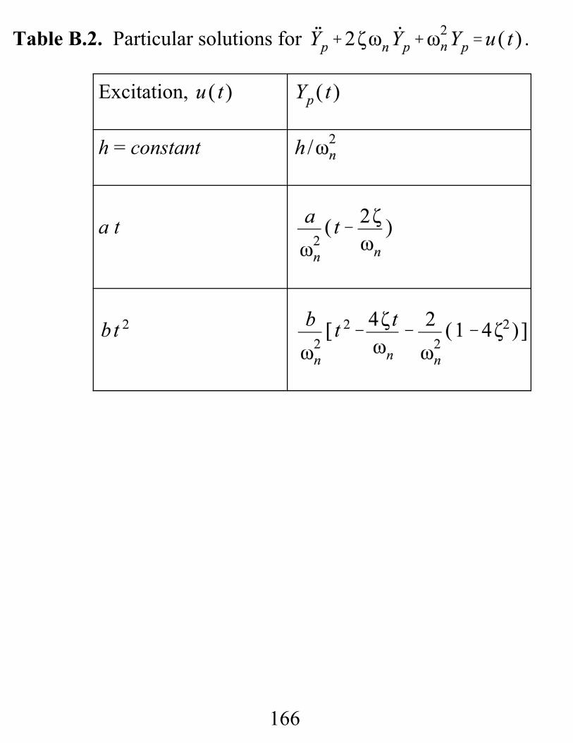
We can pick the particular solutions from Table B.2 below asfollows

166

Table B.2. Particular solutions for .

Excitation,

h = constant

a t

167

The complete solution is

The constant A is obtained via,

To obtain B, first

168

(ii)

Hence,

The complete solution satisfying the boundary conditions is

and Eq.(ii) completes Task b.

Moving towards Task c,.

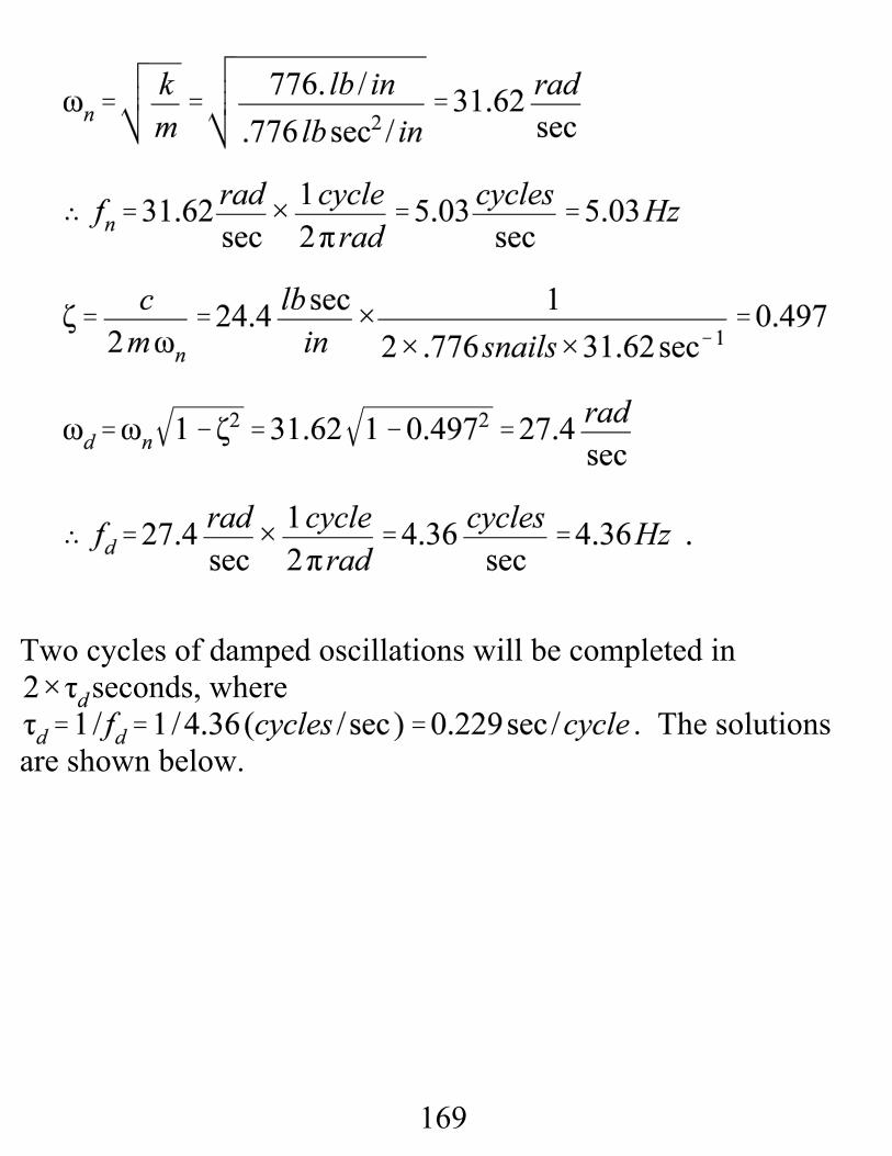
169

Two cycles of damped oscillations will be completed inseconds, where

. The solutionsare shown below.

170

x versus t

-1012345678

0 0.1 0.2 0.3 0.4 0.5

t (seconds)

x (in

ches

)

x_b -x versus t

00.010.020.030.040.050.060.070.080.090.1

0 0.1 0.2 0.3 0.4 0.5

t (seconds)

( x_b

-x )

( in

ches

)

(x dot_b-x dot) versus t

-0.4-0.20

0.20.40.60.81

1.21.4

0 0.1 0.2 0.3 0.4 0.5

t (seconds)

x do

t_b-

x do

t ( in

/ se

c )

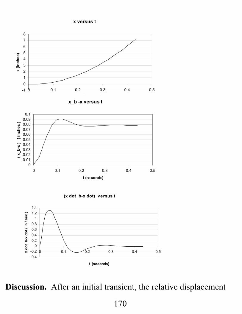
Discussion. After an initial transient, the relative displacement

171

approaches a constant value , while therelative velocity approaches zero; i.e., . The scalingfor hides the initial transient, but the plot shows quadraticincrease with time, which is consistent with its constantacceleration at . The spring force

, while the forcerequired to accelerate the mass at g/5 is

Hence, the asymptotic value for creates the spring forcerequired to accelerate the mass at .

172

(iii)

Example XP3.6Think about an initially motionless cart being “snagged” by amoving vehicle with velocity through a connection consistingof a parallel spring-damper assembly. The connecting spring isundeflected prior to contact. That circumstance can be modeledby giving the base end of the model in figure XP3.5 the velocity

; i.e., , and the governingequation of motion is

with initial conditions . The engineering analysistasks for this example are:

a. Determine the complete solution that satisfies the initialconditions.

b. For the data set, , , and, determine .

c. For produce plots for the mass displacement, relative displacement , and the mass

velocity for two cycles of motion.

173

Solution. From Table B.2, the particular solutions correspondingto the right-hand terms are:

The complete solution is

Solving for A ,

Solving for B from

174

(iv)

gives

The complete solution satisfying the initial conditions is

which completes Task a.

For Task b,

175

x versus t

0

1

2

3

4

5

6

7

0 0.2 0.4 0.6 0.8 1 1.2

t ( seconds )

x (

met

ers

)

x_b - x versus t

-0.1

-0.05

0

0.05

0.1

0.15

0.2

0.25

0 0.2 0.4 0.6 0.8 1 1.2

t ( seconds )

( x_b

- x)

( m

eter

s )

From the last of these results, the period for a damped oscillationis .

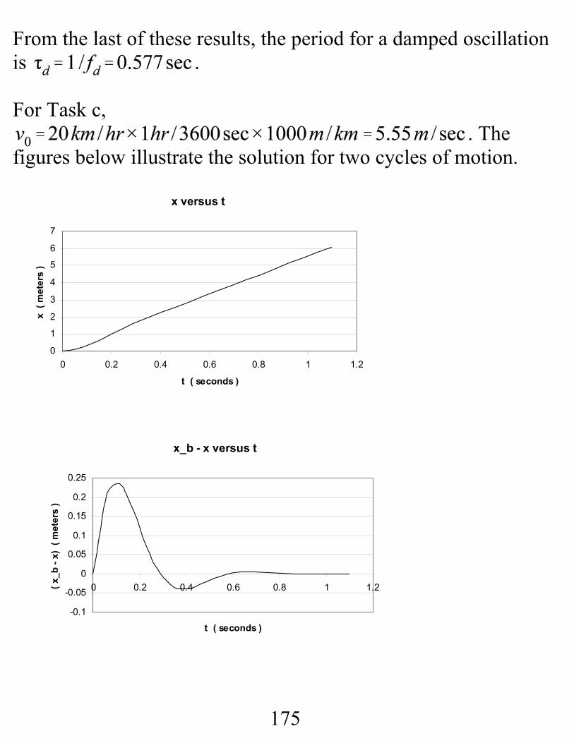
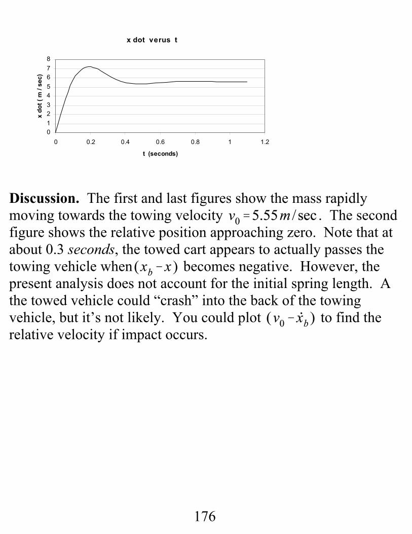
For Task c,. The

figures below illustrate the solution for two cycles of motion.

176

x dot verus t

012345678

0 0.2 0.4 0.6 0.8 1 1.2

t (seconds)

x do

t ( m

/ se

c)

Discussion. The first and last figures show the mass rapidlymoving towards the towing velocity . The secondfigure shows the relative position approaching zero. Note that atabout 0.3 seconds, the towed cart appears to actually passes thetowing vehicle when becomes negative. However, thepresent analysis does not account for the initial spring length. Athe towed vehicle could “crash” into the back of the towingvehicle, but it’s not likely. You could plot to find therelative velocity if impact occurs.

177

(3.32)

(3.33)

(3.34)

LECTURE 11. HARMONIC EXCITATION

Forced Excitation

Dividing through by the mass m gives

Seeking a particular solution for the right hand term gives

Substituting this solution into Eq.(3.32) yields

Gathering the and coefficients gives the following

178

(3.35)

two equations:

The matrix statement for the unknowns D and C is

Using Cramer’s rule for their solution gives:

where Δ is the determinant of the coefficient matrix defined by

The solution defined by Eq.(3.34) can be restated

179

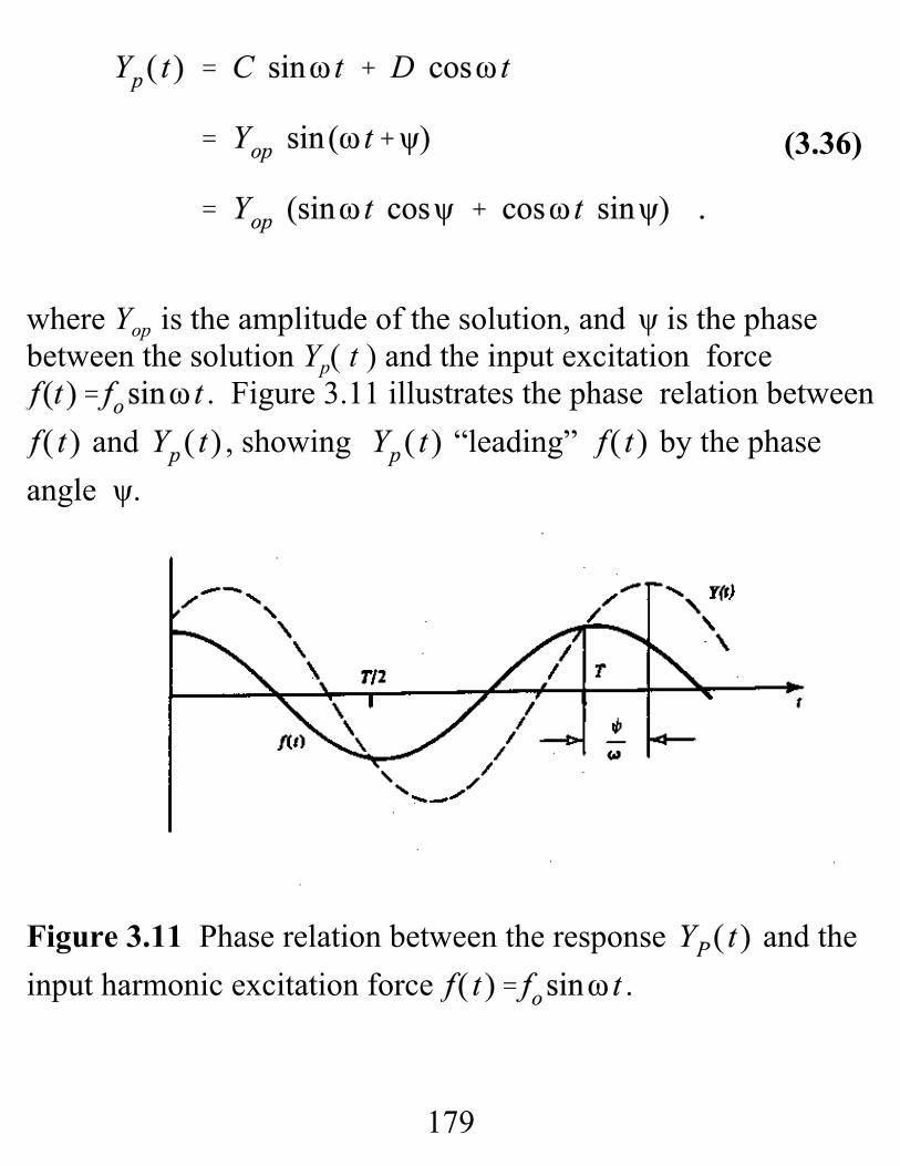
(3.36)

where Yop is the amplitude of the solution, and ψ is the phasebetween the solution Yp( t ) and the input excitation force

. Figure 3.11 illustrates the phase relation between and , showing “leading” by the phase

angle ψ.

Figure 3.11 Phase relation between the response and theinput harmonic excitation force .

180

(3.38)

The solution for C and D provided by Eq.(3.35) gives:

where

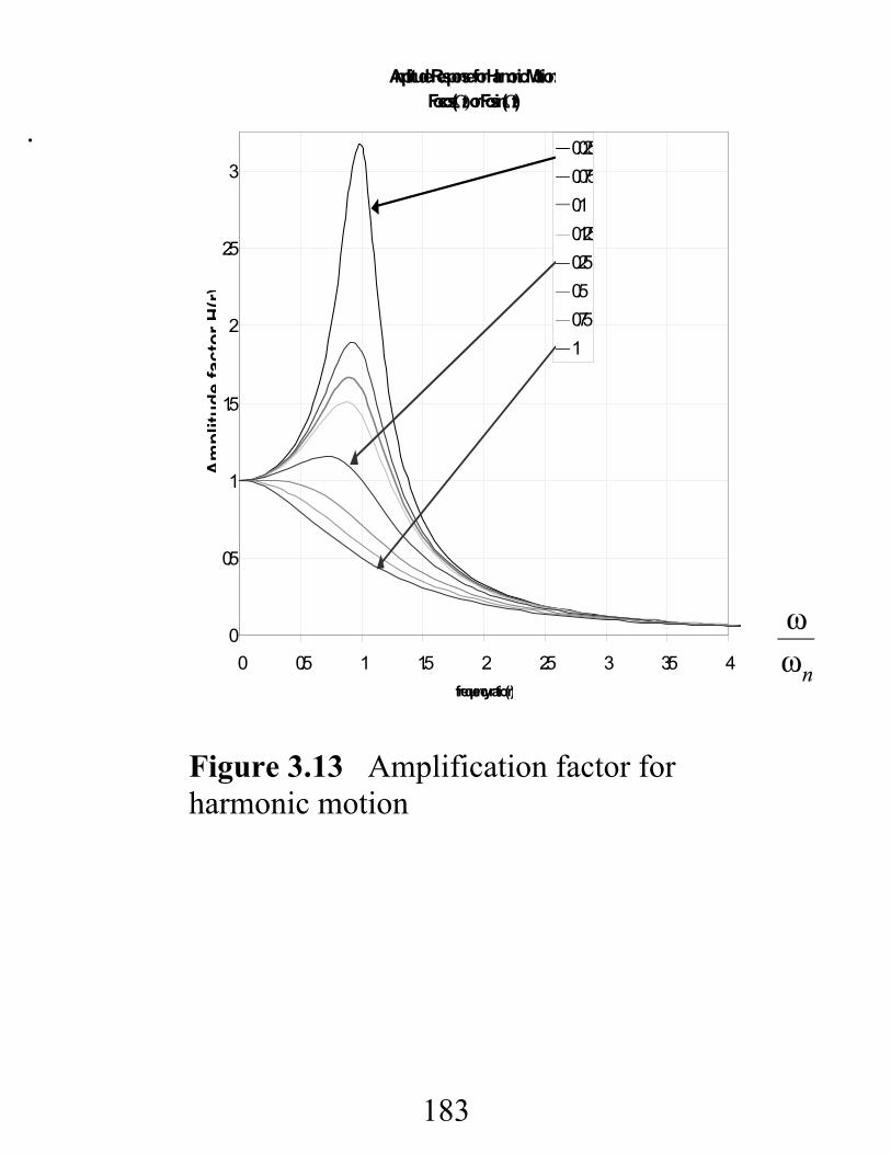
Amplification Factor

The maximum amplification factor is found from

181

(3.39)

(3.40a)

as

Note that

This is another way to characterize damping.

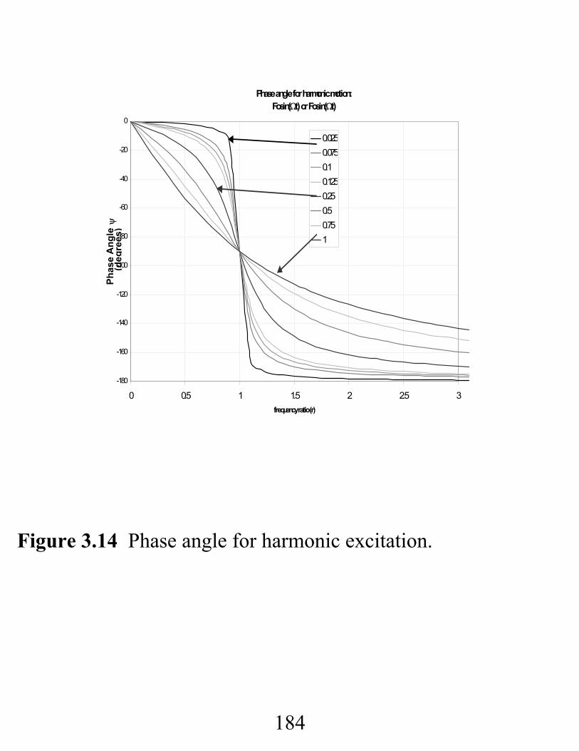
Eqs.(3.35) and (3.36) define the phase as

Complete Solution

182

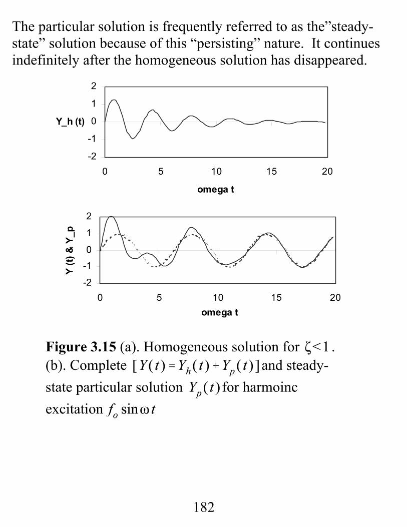
The particular solution is frequently referred to as the”steady-state” solution because of this “persisting” nature. It continuesindefinitely after the homogeneous solution has disappeared.

-2

-1

0

1

2

0 5 10 15 20

omega t

Y_h (t)

-2

-1

0

1

2

0 5 10 15 20omega t

Y (t)

& Y

_p

Figure 3.15 (a). Homogeneous solution for .(b). Complete and steady-state particular solution for harmoincexcitation

183

.

Amplitude Response for Harmonic Motion:Focos(Ωt) or Fosin(Ωt)

0

0.5

1

1.5

2

2.5

3

0 0.5 1 1.5 2 2.5 3 3.5 4frequency ratio (r)

Am

plitu

defa

ctor

H(r

)

0.0250.0750.10.1250.250.50.751

Figure 3.13 Amplification factor forharmonic motion

184

Figure 3.14 Phase angle for harmonic excitation.

Phase angle for harmonic motion:Fosin(Ωt) or Fosin(Ωt)

-180

-160

-140

-120

-100

-80

-60

-40

-20

0

0 0.5 1 1.5 2 2.5 3frequency ratio (r)

Phas

e A

ngle

ψ (d

egre

es)

0.0250.0750.10.1250.250.50.751

185

(i)

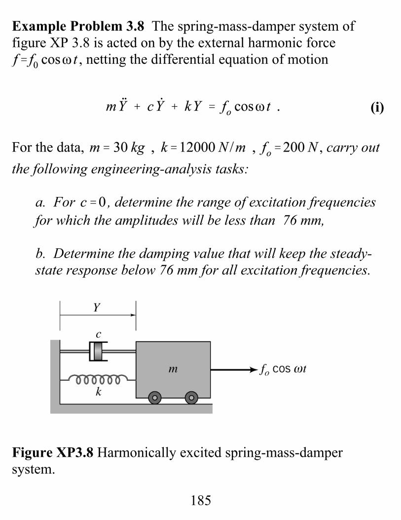
Example Problem 3.8 The spring-mass-damper system offigure XP 3.8 is acted on by the external harmonic force

, netting the differential equation of motion

For the data, , carry outthe following engineering-analysis tasks:

a. For , determine the range of excitation frequenciesfor which the amplitudes will be less than 76 mm,

b. Determine the damping value that will keep the steady-state response below 76 mm for all excitation frequencies.

Figure XP3.8 Harmonically excited spring-mass-dampersystem.

186

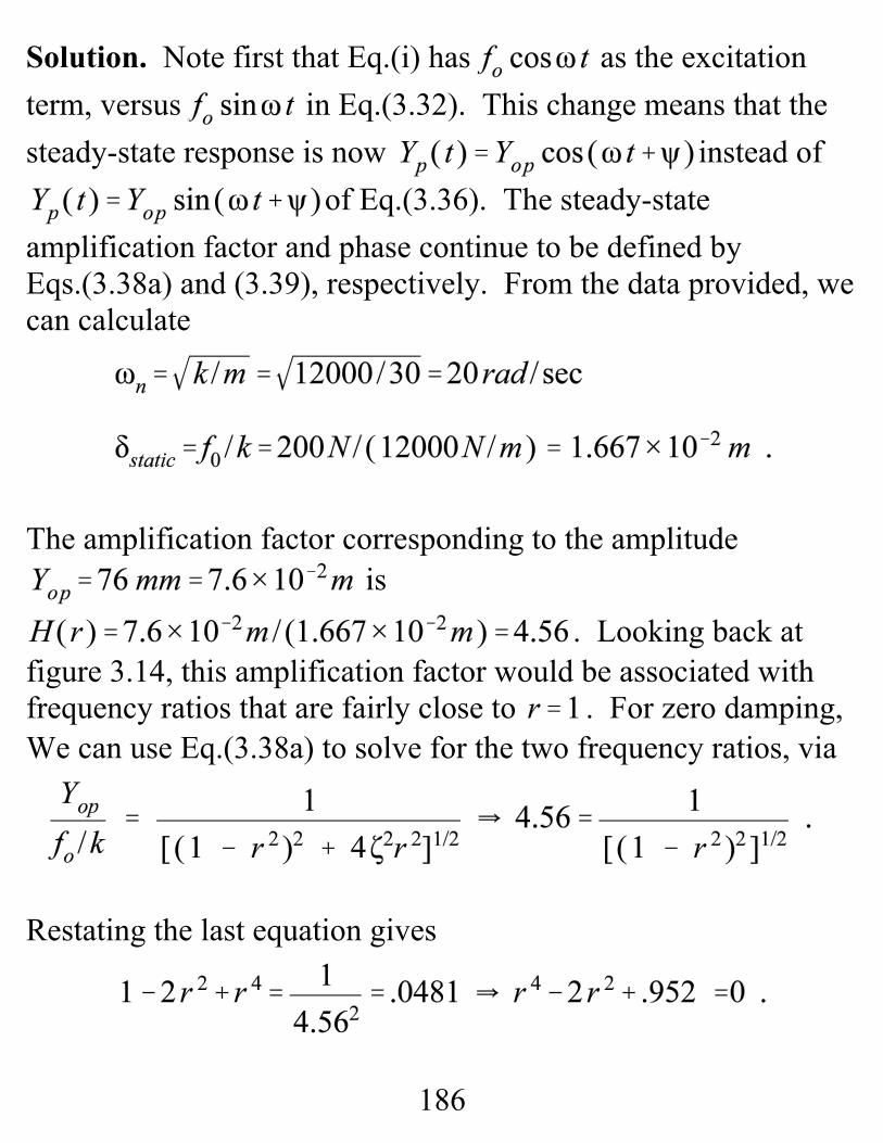
Solution. Note first that Eq.(i) has as the excitationterm, versus in Eq.(3.32). This change means that thesteady-state response is now instead of

of Eq.(3.36). The steady-stateamplification factor and phase continue to be defined byEqs.(3.38a) and (3.39), respectively. From the data provided, wecan calculate

The amplification factor corresponding to the amplitude is

. Looking back atfigure 3.14, this amplification factor would be associated withfrequency ratios that are fairly close to . For zero damping,We can use Eq.(3.38a) to solve for the two frequency ratios, via

Restating the last equation gives

187

Solving this quadratic equation defines the two frequencies by:

As expected, and are close to the natural frequency . The steady-state amplitudes will be less than the specified 76mm , for the frequency ranges, and

, and we have competed Task a.

Moving to Task b, the amplification factor is a maximum at, and its maximum value is .

Hence,

and the required damping to achieve this ζ value is, fromEq.(3.22),

188

Note that the derived units for the newton is ; hence, . Damping coefficients of this value orhigher will keep the peak response amplitudes at less than thespecified 76 mm, and Task b is completed.

Figure 3.15. (a). Suspended mass and movable base. (b). Free-body diagram for tension in the springs and damper, (c). Free-body diagram for compression in the springs and damper.

189

(3.42)

(3.43)

(3.41)

Harmonic Base Excitation. Base harmonic base motion can bedefined by , , and

becomes

Dividing through by m gives

We can solve for B and φ from the last two lines of this equation,obtaining

Looking at Eq.(3.41), our sole interest is the steady-state solutiondue to the harmonic excitation term .

Based on the earlier results of Eq.(3.36), the expected steady-state solution format to Eq.(3.41) is

190

(3.44)

with ψ defined by Eq.(3.39). This solution is sinusoidal at theinput frequency ω, having the same phase lag ψ with respect tothe input force excitation as determined earlier forthe harmonic force excitation .

Comparison Eqs.(3.33) and (3.41), shows B replacing . Substituting into Eq.(3.37) gives

Hence, the ratio of the steady-state-response amplitude to thebase-excitation amplitude is

Figure 3.16 illustrates , showing a strong similarity toof figure 3.13 with the peak amplitudes occurring near

. For , the two transfer functions coincide. Themaximium for is obtained via , yielding

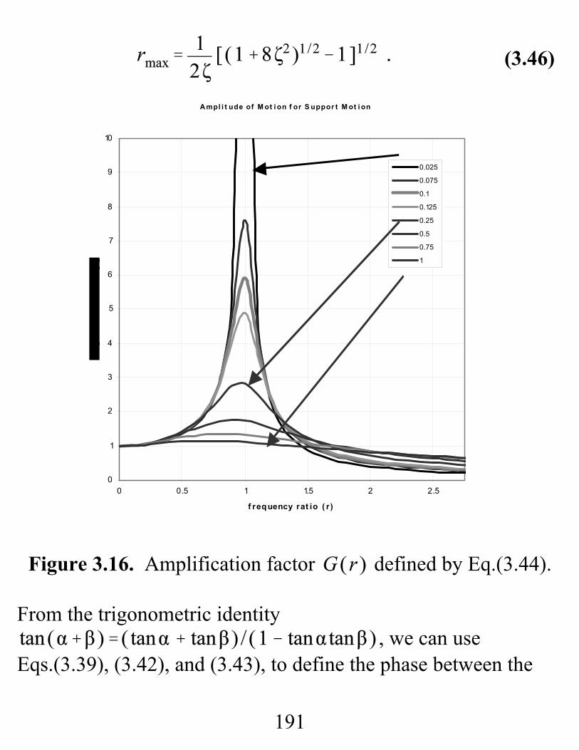
191

(3.46)

Figure 3.16. Amplification factor defined by Eq.(3.44).

From the trigonometric identity , we can use

Eqs.(3.39), (3.42), and (3.43), to define the phase between the

A mpl i t ude of M ot i on f or S uppor t M ot i on

0

1

2

3

4

5

6

7

8

9

10

0 0.5 1 1.5 2 2.5

f requency rat io ( r )

0.025

0.075

0.1

0.125

0.25

0.5

0.75

1

192

(3.45)

steady-state solution and the basemotion excitation as

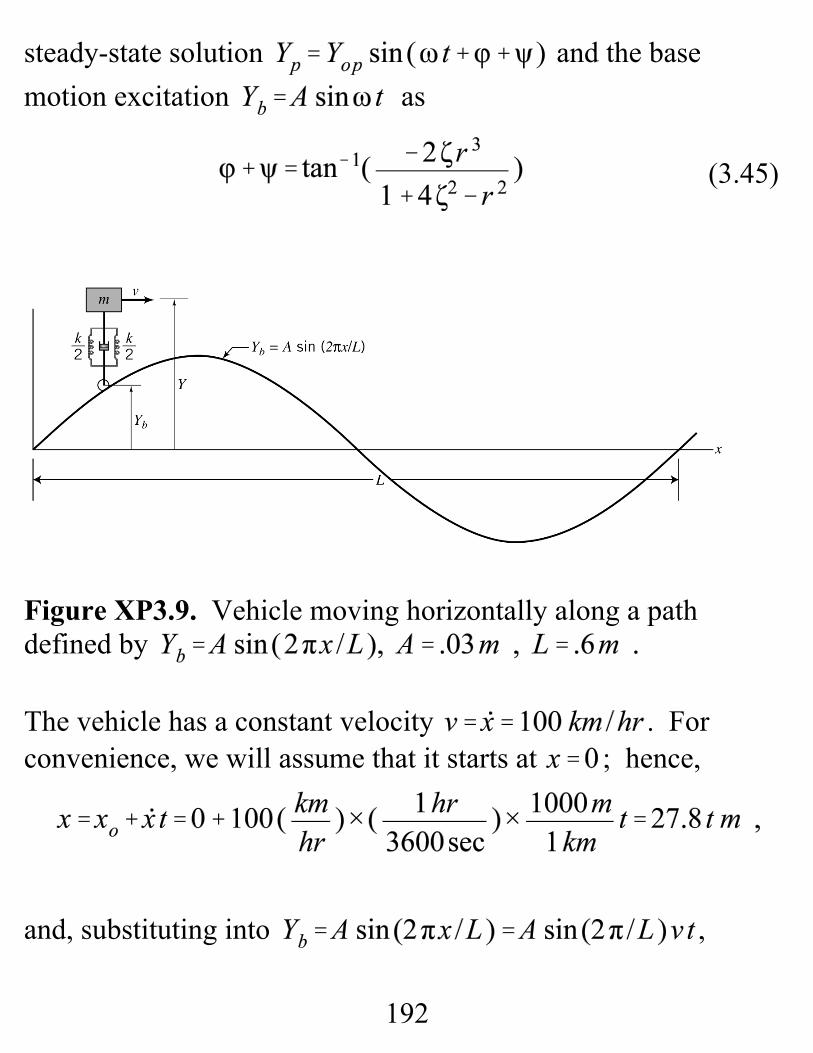
Figure XP3.9. Vehicle moving horizontally along a pathdefined by

The vehicle has a constant velocity . Forconvenience, we will assume that it starts at ; hence,

and, substituting into ,

193

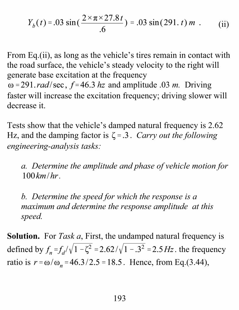
(ii)

From Eq.(ii), as long as the vehicle’s tires remain in contact withthe road surface, the vehicle’s steady velocity to the right willgenerate base excitation at the frequency

and amplitude .03 m. Drivingfaster will increase the excitation frequency; driving slower willdecrease it.

Tests show that the vehicle’s damped natural frequency is 2.62Hz, and the damping factor is . Carry out the followingengineering-analysis tasks:

a. Determine the amplitude and phase of vehicle motion for.

b. Determine the speed for which the response is amaximum and determine the response amplitude at thisspeed.

Solution. For Task a, First, the undamped natural frequency isdefined by . the frequencyratio is . Hence, from Eq.(3.44),

194

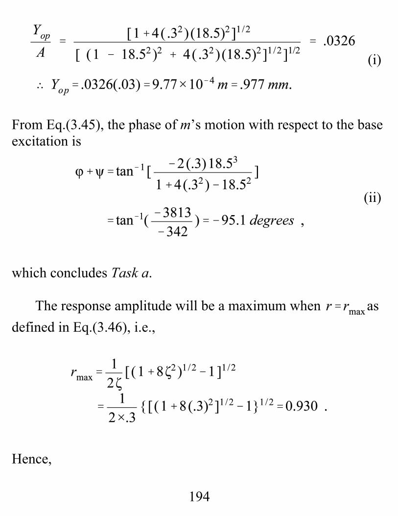
(i)

(ii)

From Eq.(3.45), the phase of m’s motion with respect to the baseexcitation is

which concludes Task a.

The response amplitude will be a maximum when asdefined in Eq.(3.46), i.e.,

Hence,

195

From Eq.(3.45), at this speed, the steady-state amplificationfactor is

196

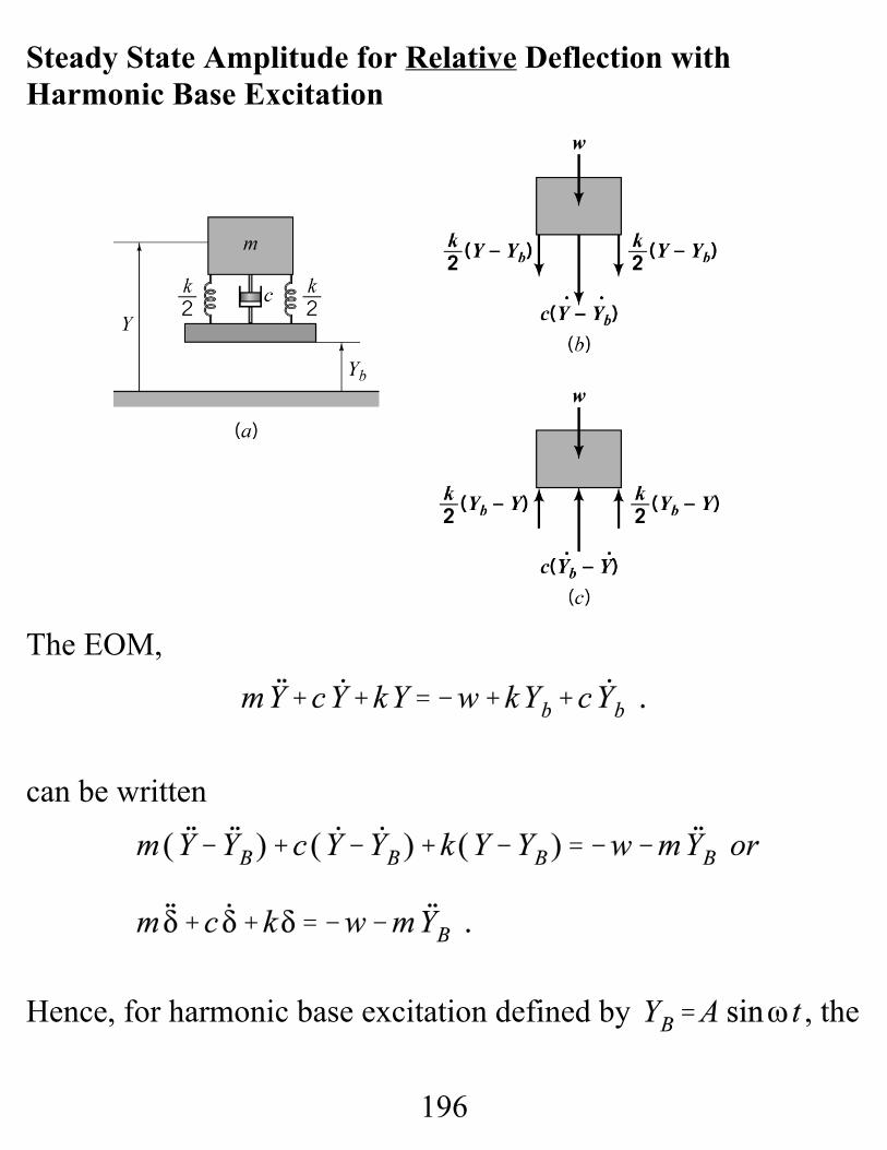
Steady State Amplitude for Relative Deflection withHarmonic Base Excitation

The EOM,

can be written

Hence, for harmonic base excitation defined by , the

197

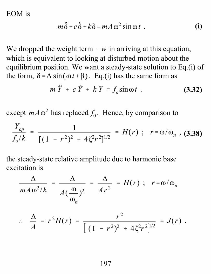
(3.32)

(3.38)

EOM is

We dropped the weight term in arriving at this equation,which is equivalent to looking at disturbed motion about theequilibrium position. We want a steady-state solution to Eq.(i) ofthe form, . Eq.(i) has the same form as

except has replaced . Hence, by comparison to

the steady-state relative amplitude due to harmonic baseexcitation is

(i)

198

Figure 3.18. versus frequency ratio fromEq.(3.49) for a range of damping ratio values.

Example Problem 3.9 Revisited. Solve for the steady-staterelative amplitude at as

This value is much greater than the absolute amplitude of motion

Amplitude Response for Rotating Imbalance

0

1

2

3

4

5

6

7

8

9

10

0 0.5 1 1.5 2 2.5

frequency ratio (r)

Am

plitu

de fa

ctor

J(r

)0.0250.0750.10.1250.250.50.751

199

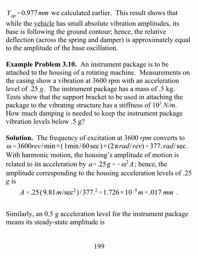
we calculated earlier. This result shows thatwhile the vehicle has small absolute vibration amplitudes, itsbase is following the ground contour; hence, the relativedeflection (across the spring and damper) is approximately equalto the amplitude of the base oscillation.

Example Problem 3.10. An instrument package is to beattached to the housing of a rotating machine. Measurements onthe casing show a vibration at 3600 rpm with an accelerationlevel of .25 g. The instrument package has a mass of .5 kg. Tests show that the support bracket to be used in attaching thepackage to the vibrating structure has a stiffness of 105 N/m. How much damping is needed to keep the instrument packagevibration levels below .5 g?

Solution. The frequency of excitation at 3600 rpm converts to.

With harmonic motion, the housing’s amplitude of motion isrelated to its acceleration by ; hence, theamplitude corresponding to the housing acceleration levels of .25g is

Similarly, an 0.5 g acceleration level for the instrument packagemeans its steady-state amplitude is

200

Hence, the target amplification factor is .

The natural frequency of the instrument package is

Hence, the frequency ratio is .

Plugging into Eq.(3.44) gives

The solution to this equation is . Hence, therequired damping is

which concludes the engineering-analysis task. Note that thederived units for the Newton are ; hence, nets

. Note that, since only one excitation frequency isinvolved, we could have simply taken the ratio of the

201

acceleration levels directly to get .

202

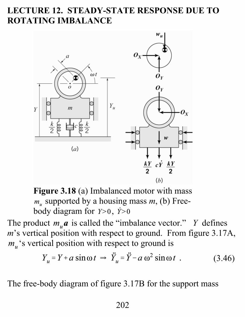
Figure 3.18 (a) Imbalanced motor with mass supported by a housing mass m, (b) Free-

body diagram for ,

(3.46)

LECTURE 12. STEADY-STATE RESPONSE DUE TOROTATING IMBALANCE

The product is called the “imbalance vector.” Y definesm’s vertical position with respect to ground. From figure 3.17A,

‘s vertical position with respect to ground is

The free-body diagram of figure 3.17B for the support mass

203

(3.32)

(3.47)

(3.48a)

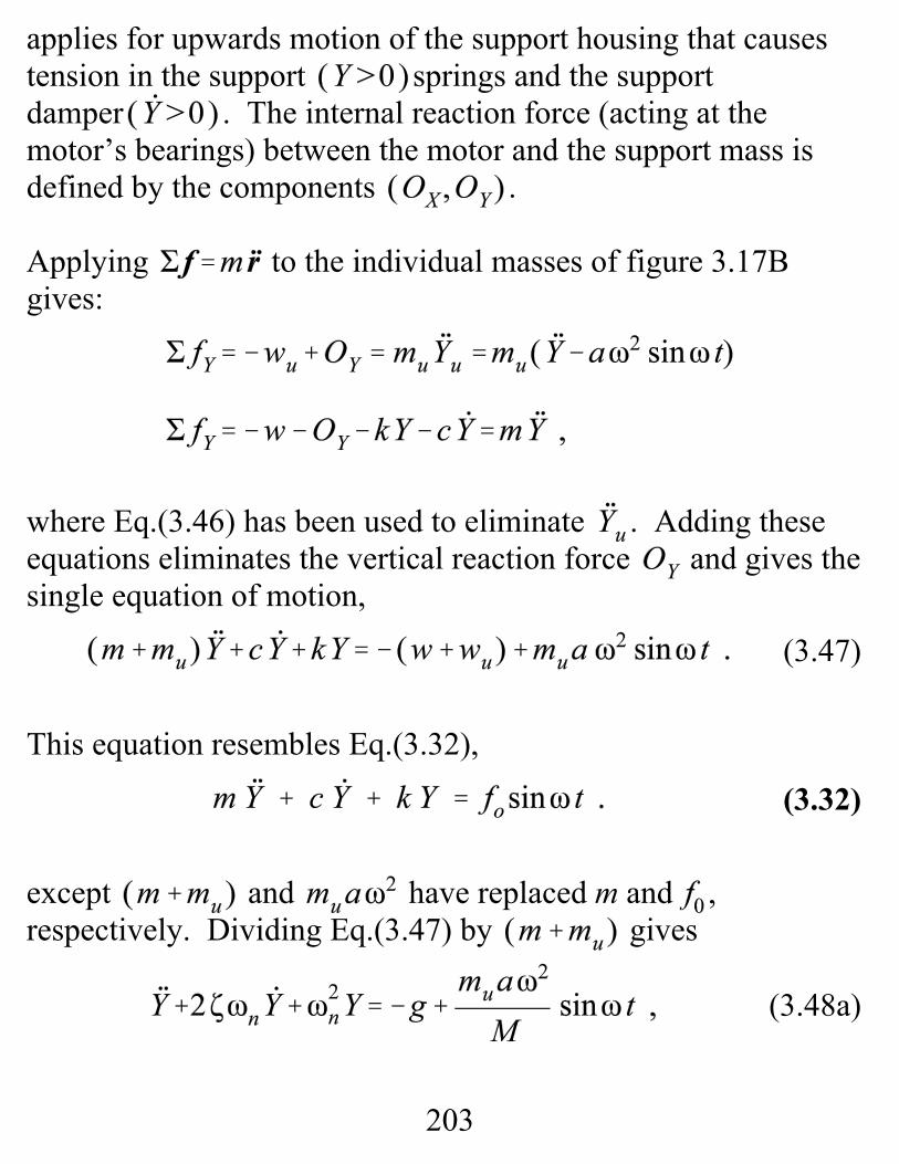
applies for upwards motion of the support housing that causestension in the support springs and the supportdamper . The internal reaction force (acting at themotor’s bearings) between the motor and the support mass isdefined by the components .

Applying to the individual masses of figure 3.17Bgives:

where Eq.(3.46) has been used to eliminate . Adding theseequations eliminates the vertical reaction force and gives thesingle equation of motion,

This equation resembles Eq.(3.32),

except and have replaced m and ,respectively. Dividing Eq.(3.47) by gives

204

(3.48b)

(3.37)

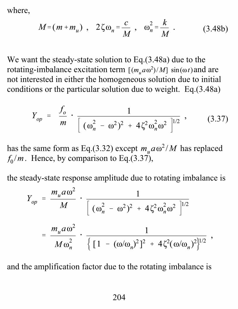
where,

We want the steady-state solution to Eq.(3.48a) due to therotating-imbalance excitation term and arenot interested in either the homogeneous solution due to initialconditions or the particular solution due to weight. Eq.(3.48a)

has the same form as Eq.(3.32) except has replaced. Hence, by comparison to Eq.(3.37),

the steady-state response amplitude due to rotating imbalance is

and the amplification factor due to the rotating imbalance is

205

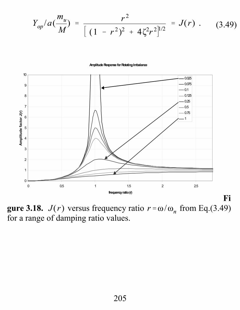
(3.49)

Figure 3.18. versus frequency ratio from Eq.(3.49)for a range of damping ratio values.

Amplitude Response for Rotating Imbalance

0

1

2

3

4

5

6

7

8

9

10

0 0.5 1 1.5 2 2.5

frequency ratio (r)

Am

plitu

de fa

ctor

J(r

)

0.0250.0750.10.1250.250.50.751

206

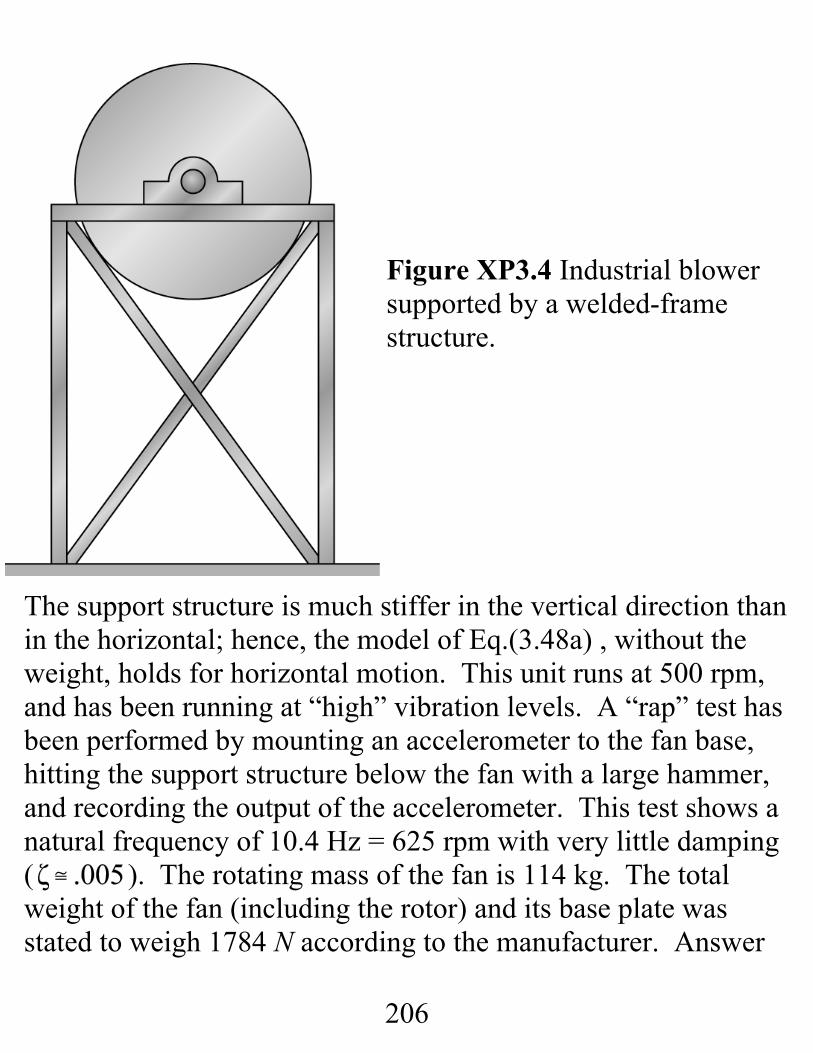
Figure XP3.4 Industrial blowersupported by a welded-framestructure.

The support structure is much stiffer in the vertical direction thanin the horizontal; hence, the model of Eq.(3.48a) , without theweight, holds for horizontal motion. This unit runs at 500 rpm,and has been running at “high” vibration levels. A “rap” test hasbeen performed by mounting an accelerometer to the fan base,hitting the support structure below the fan with a large hammer,and recording the output of the accelerometer. This test shows anatural frequency of 10.4 Hz = 625 rpm with very little damping( ). The rotating mass of the fan is 114 kg. The totalweight of the fan (including the rotor) and its base plate wasstated to weigh 1784 N according to the manufacturer. Answer

207

the following questions:

a. Assuming that the vibration level on the fan is to be lessthan , how well should the fan be balanced; i.e., to whatvalue should a be reduced?

b. Assuming that the support structure could be stiffenedlaterally by approximately 50%, how well should the fan bebalanced?

Solution. In terms of the steady-state amplitude of the housing,the housing acceleration magnitude is ,where . Hence, at

the housing-amplitude specification is:

Applying the notation of Eq.(3.49) gives

and . Applying Eq.(3.49) gives

208

Hence, the imbalance vector magnitude a should be no morethan

which concludes Task a. Balancing and maintaining the rotorsuch that for a 114 kg fan rotor is not easy.

Moving to Task b, and assuming that the structural stiffeningdoes not appreciably increase the mass of the fan assembly,increasing the lateral stiffness by 50% would change the naturalfrequency to

With a stiffened housing, ,. Since ,

Hence,

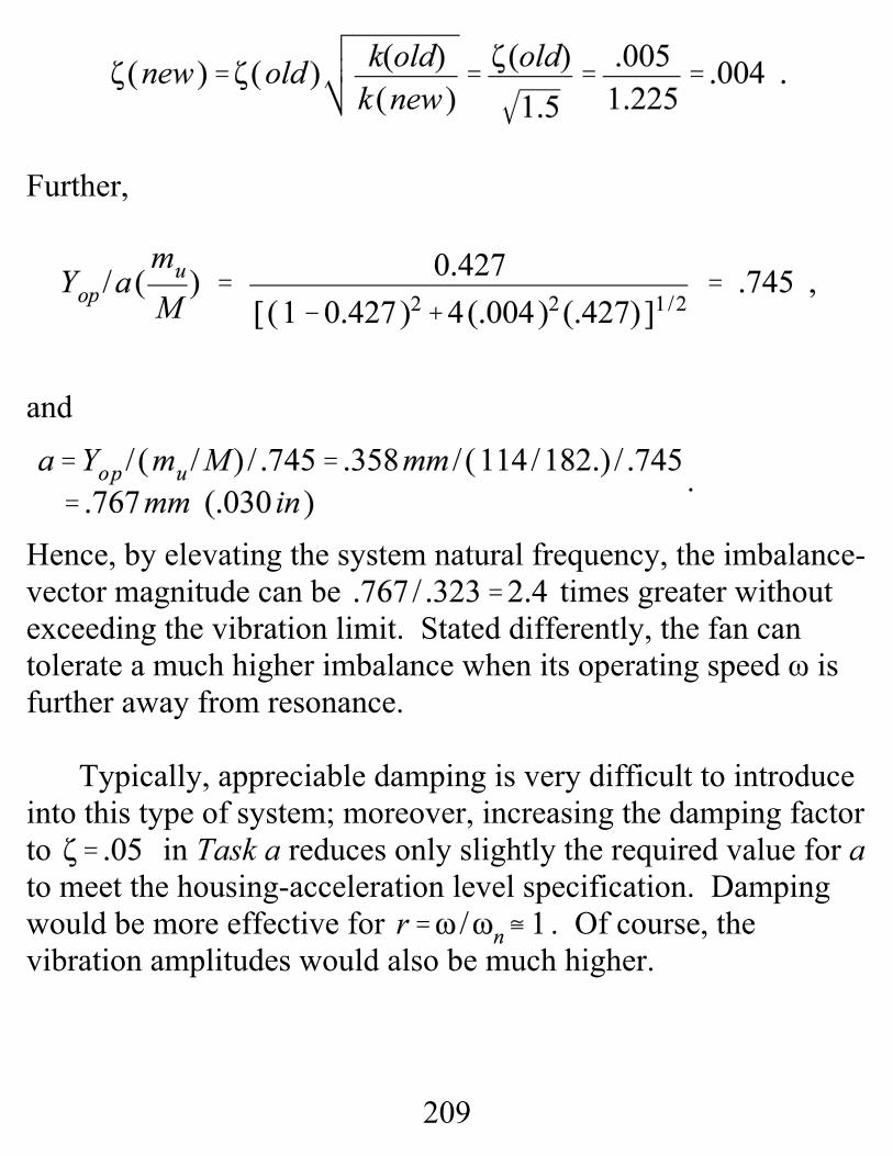
209

Further,

and

.

Hence, by elevating the system natural frequency, the imbalance-vector magnitude can be times greater withoutexceeding the vibration limit. Stated differently, the fan cantolerate a much higher imbalance when its operating speed ω isfurther away from resonance.

Typically, appreciable damping is very difficult to introduceinto this type of system; moreover, increasing the damping factorto in Task a reduces only slightly the required value for a to meet the housing-acceleration level specification. Dampingwould be more effective for . Of course, thevibration amplitudes would also be much higher.

210

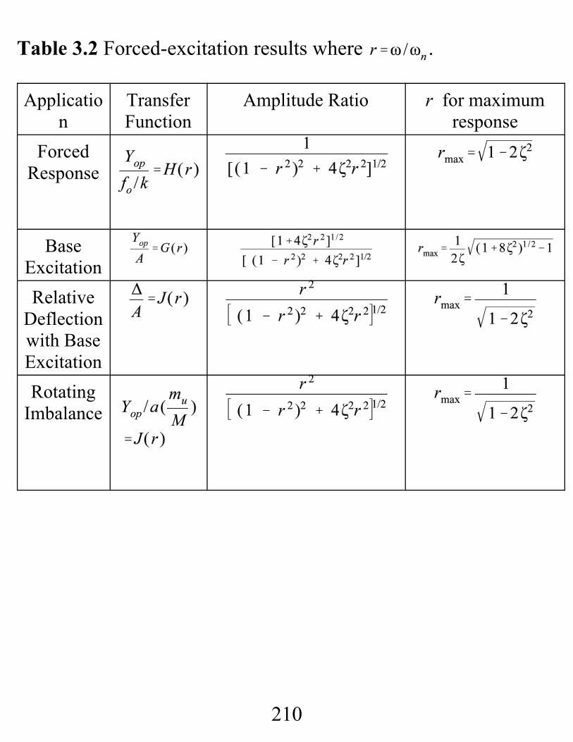
Table 3.2 Forced-excitation results where .

Application

TransferFunction

Amplitude Ratio r for maximumresponse

ForcedResponse

BaseExcitationRelative

Deflectionwith BaseExcitationRotating

Imbalance