Finite Volume Model for Two-Dimensional Shallow …Finite Volume Model for Two-Dimensional Shallow...

loped fors, whichond-ordermall waterinishingapplied to

Finite Volume Model for Two-Dimensional Shallow WaterFlows on Unstructured Grids

Tae Hoon Yoon, F.ASCE,1 and Seok-Koo Kang2

Abstract: A numerical model based upon a second-order upwind finite volume method on unstructured triangular grids is devesolving shallow water equations. The HLL approximate Riemann solver is used for the computation of inviscid flux functionmakes it possible to handle discontinuous solutions. A multidimensional slope-limiting technique is employed to achieve secspatial accuracy and to prevent spurious oscillations. To alleviate the problems associated with numerical instabilities due to sdepths near a wet/dry boundary, the friction source terms are treated in a fully implicit way. A third-order total variation dimRunge–Kutta method is used for the time integration of semidiscrete equations. The developed numerical model has beenseveral test cases as well as to real flows. Numerical tests prove the robustness and accuracy of the model.

DOI: 10.1061/~ASCE!0733-9429~2004!130:7~678!

CE Database subject headings: Floods; Hydraulic models; Numerical models; Shallow waters; Unsteady flow.

plexf theen-duceeom-suchl nu-backsex-

idely, andevel-ethod

Molls

hanen

lvedore

e-prob-

ener-two-s is

o in-ionsch-plex

nted tousing

naleth-

euredward

rob-ld.erleighthe

thethenaled onrids

olverder

ysicaland

seda-

andtionecon-

ma--100;ea.

ndaieup,8@

ssionste bygingpos-

er 25,

4/7-

Introduction

Flows in rivers, floodplains, and coastal zones are very comdue to uneven bottom topography and irregular boundaries oflow domain. These cannot be easily solved by the unidimsional models and even the bidimensional models cannot proaccurate results if they are not able to handle complicated getries or are not robust enough to treat abrupt flow changesas shocks and discontinuities or dry bed conditions. Severamerical schemes have been developed to alleviate the drawinvolved in the bidimensional models but it seems that thereists no an all-around model so far.

Two-dimensional shallow water equations have been wused to simulate flows in shallow lakes, wide rivers, estuariescoastal zones. A number of numerical methods have been doped to solve these equations, such as the finite difference m~Garcia and Kahawita 1986; Fennema and Chaudhry 1990;and Chaudhry 1995!, the finite element method~Akanbi andKatopodes 1988!, and the finite volume method~Alcrudo andGarcia-Navarro 1993; Zhao et al. 1994; Anastasiou and C1997; Sleigh et al. 1998!. The finite difference methods have beused with structured grids that permit the flow field to be soefficiently. Structured grids, which make the flow solver m

1Professor Emeritus, Han River Eco-Hydro Inst., 367-6 ChunOksoo Bldg. 3F, Oksoo-dong, Sungdong-gu, Seoul, Korea 133formerly, Dept. of Civil Engineering, Hanyang Univ., Seoul, KorE-mail: [email protected]

2Researcher, Hyundai Institute of Construction Technology, HyuEngineering & Construction, Co. Ltd., 102-4, Mabuk-ri, Goosung-Yongin, Kyeong-gi-do, Korea 449-716. E-mail: kangsk7ihanyang.ac.kr

Note. Discussion open until December 1, 2004. Separate discumust be submitted for individual papers. To extend the closing daone month, a written request must be filed with the ASCE ManaEditor. The manuscript for this paper was submitted for review andsible publication on September 17, 2002; approved on Septemb2003. This paper is part of theJournal of Hydraulic Engineering, Vol.130, No. 7, July 1, 2004. ©ASCE, ISSN 0733-9429/200
678–688/$18.00.
678 / JOURNAL OF HYDRAULIC ENGINEERING © ASCE / JULY 2004

Downloaded 10 Nov 2010 to 198.91.37.2. Redistribution

efficient, may confront difficulties in modeling complex flow gometries. In these cases, unstructured grids can alleviate thelems associated with structured grids. A triangular mesh is gally the simplest and most convenient way for covering adimensional domain. An advantage of using triangular gridtheir ability to generate grids on arbitrary geometries and tcrease the number of cells in high-gradient regions or in regof particular interest in the flow field. It is a quite attractive tenique for modeling rivers or coastal zones because the comgeometry is intractable when using structured grids.

Recently, several successful schemes have been presesolve the shallow water equations on unstructured grids byfinite volume formulations. Anastasiou and Chan~1997! andSleigh et al.~1998! reported a solution of the two-dimensioshallow water equations using second-order finite volume mods on triangular meshes. Zhao et al.~1994! developed a finitvolume model with first-order spatial accuracy on unstructmeshes. Currently, there has not been much work done toapplying unstructured finite volume methods to real flow plems and verifying their capability to predict the real flow fieZhao et al.~1994! applied their model to the Kissimmee Rivbasin in the United States reporting satisfactory results. Set al. ~1998! applied a second-order finite volume method toAxe estuary in the United Kingdom.

In an attempt to circumvent many difficulties present inexisting numerical models and to verify the applicability offinite volume method to real flow problems, a two-dimensiomodel is proposed and tested in this paper. The model is basthe upwind finite volume method on unstructured triangular gand employs a cell-centered finite volume formulation to sconservative two-dimensional shallow water equations. In oto achieve high-order spatial accuracy and to prevent nonphoscillations, the multidimensional reconstruction techniquethe continuously differentiable multidimensional limiter propoby Jawahar and Kamath~2000! are employed in this study. Jawhar and Kamath~2000! applied the reconstruction techniquethe limiter to solve the two-dimensional linear advection equaand compressible Euler and Navier–Stokes equations. The r
struction technique is based on a wide computational stencil and
subject to ASCE license or copyright. Visit http://www.ascelibrary.org

ty forbleumpswith

reti-ing

tinu-aces.lit-mall

tionsr theis-ro-tinu-

,y;

y.an-

flu-stresslected

ntll and

left-the

lines

l,the

he-r ap-

trol

does not strongly depend on vertex values to preserve stabilihighly distorted grids. The limiter is continuously differentiaand produces a smooth transition between discontinuous jwith first-order accuracy and sharp but continuous gradientssecond-order accuracy.

To accomplish high-order temporal accuracy, the time disczation is made by the third-order total variation diminish~TVD! Runge–Kutta method~Shu and Osher 1988!. The HLLapproximate Riemann solver enabling one to handle disconous solutions is used to evaluate inviscid fluxes at the cell fThe friction terms are treated fully implicitly by an operator spting technique to prevent numerical instabilities caused by a swater depth near the dry zones.

Governing Equations

The two-dimensional depth-integrated shallow water equaare obtained by integrating the Navier–Stokes equations oveflow depth with the following assumptions: uniform velocity dtribution in the vertical direction, incompressible fluid, hydstatic pressure distribution, and small bottom slope. The conity and momentum equations are

]U]t

1]F]x

1]G]y

5S (1)

in which

U5S huhvh

D , F5S uhu2h1gh2/2

uvhD , G5S vh

uvhv2h1gh2/2

Dand

S5So1Sf5S 0ghSox

ghSoy

D 1S 02ghSf x

2ghSf y

D (2)

whereu and v5velocity components in thex and y directionsrespectively; h5water depth; g5acceleration due to gravit(Sox ,Soy)5bed slopes in the x and y directions, and(Sf x ,Sf y)5friction slopes in thex andy directions, respectivelIn this study, the friction slopes are estimated by using the Mning formula

Sf x5n2uAu21v2

h4/3, Sf y5

n2vAu21v2

h4/3

where n5Manning’s roughness coefficient. In general, the inence of bottom roughness prevails over the turbulent shearbetween cells. Therefore the effective stress terms were negin the computation.

where (UL) i , j and (UR) i , j5reconstructions ofU on the left and right

JO


Numerical Model

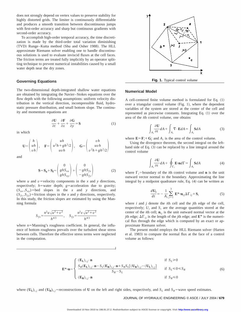
A cell-centered finite volume method is formulated for Eq.~1!over a triangular control volume~Fig. 1!, where the dependevariables of the system are stored at the center of the cerepresented as piecewise constants. Integrating Eq.~1! over thearea of theith control volume, one obtains

EAi

]U]t

dA1EAi

¹•EdA5EAi

SdA (3)

whereE5Fi 1G j andAi is the area of the control volume.Using the divergence theorem, the second integral on the

hand side of Eq.~3! can be replaced by a line integral aroundcontrol volume

EAi

]U]t

dA1 RG i

E"ndG5EAi

SdA (4)

whereG i5boundary of theith control volume andn is the unitoutward vector normal to the boundary. Approximating theintegral by a midpoint quadrature rule, Eq.~4! can be written a

dUi

dt52

1

Ai(j 51

3

E* "ni j DG i j 1Si (5)

where i and j denote theith cell and thejth edge of the celrespectively;Ui and Si are the average quantities stored atcenter of theith cell; ni j is the unit outward normal vector at tjth edge;DG i j is the length of thejth edge; andE* is the numerical flux through the edge which is computed by an exact oproximate Riemann solver.

The present model employs the HLL Riemann solver~Hartenet al. 1983! to compute the normal flux at the face of a convolume as follows:

Fig. 1. Typical control volume

E* "n5H ~EL ! i , j•n if SL>0

SR~EL ! i , j•n2SL~ER! i , j•n1SRSL@~UR! i , j2~UL ! i , j #

SR2SLif SL<0<SR

~ER! i , j•n if SR<0

(6)

sides, respectively, andSL andSR5wave speed estimates.

URNAL OF HYDRAULIC ENGINEERING © ASCE / JULY 2004 / 679


There are several possible choices forSL andSR . The approach proposed by Toro~1992! is used in the present model:

SL5H min~qL•n2AghL,u* 2Agh* ! if both sides are wet

qL•n2AghL if the right side is dry

qR•n22AghR if the left side is dry

(7)

SR5H max~qR•n2AghR,u* 1Agh* ! if both sides are wet

qL•n12AghL if the right side is dry

qR•n1AghR if the left side is dry

(8)

u* 51

2~qL1qR!•n1AghL2AghR (9)

Agh* 51

2~AghL1AghR!1

1

4~qL2qR!•n (10)

lver,s re-pre-

iece-hichason

ent-

allowd

Liut anf ele-one-L ap-ndend onction

es noghly

form

nd

gle

this

nneltex

thef the

e

nearsicalles.

whereq5@u v#T.

Linear Reconstruction

Accuracy, which is the most important aspect for any flow sohas a direct influence on the number of computational cellquired to resolve a flow field as economically as possible. Resenting the numerical approximation of the solution as a pwise constant is equivalent to a first-order spatial accuracy, wis often inadequate to achieve a desired accuracy. For this rea higher-order implementation, which involves a gradireconstruction, is necessary.

There are several higher-order schemes applied to shwater equations on unstructured triangular grids~Anastasiou anChan 1997; Sleigh et al. 1998; Hubbard 1999; Wang and2000!. A high-order reconstruction on unstructured grids is noeasy task since the positions of vertices and the numbers oments surrounding a vertex are arbitrary. Extensions ofdimensional reconstruction techniques, such as the MUSCproach, to unstructured grids make the scheme strongly depeon grid connectivity, and therefore poor results are obtainehighly distorted grids. In the present study, the reconstrutechnique proposed by Jawahar and Kamath~2000!, which pos-sesses dependence on a wide computational stencil and dostrongly depend on vertex values to preserve stability for hidistorted triangles, is employed.

The initial data at each time step are reconstructed in the

Uinew5Ui1r i•¹Ui

1 (11)

wherer i5position vector relative to the centroid of the cell a¹Ui

15limited gradient.For examples, the gradient ofU for the two trianglesD1a2

and D1i2 in Fig. 1, which are referred to as (¹U)1a2 and(¹U)1i2 , can be computed using the Green–Gauss theorem

¹U51

A RGUndG (12)

where G5integration path connecting vertices of each trianandA is the area of the triangle.

In order to calculate gradients (¹U)1a2 and (¹U)1i2 , a valueof a conserved variable at a vertex should be known. For
purpose, a linearity preserving interpolation method based on the


,

t

t

pseudo-Laplacian formula proposed by Holmes and Co~1989! is used to calculate vertex values. Assuming that verkis surrounded byM cells, the conserved variable at vertexk iscalculated as follows:

Uk5(i 51

Mv i

( i 51M v i

Ui . (13)

where

v i511lx~xi2xk!1ly~yi2yk! (14)

lx5I xyRy2I yyRx

I xxI yy2I xy2

, lx5I xyRx2I xxRy

I xxI yy2I xy2

(15)

I xx5(i 51

M

~xi2xk!2, I yy5(i 51

M

~yi2yk!2,

(16)

I xy5(i 51

M

~xi2xk!~yi2yk!

Rx5(i 51

M

~xi2xk!, Ry5(i 51

M

~yi2yk! (17)

After (¹U)1a2 and (¹U)1i2 are obtained, the gradient atface j 51 is computed by using the area-weighted average otwo trianglesD1a2 andD1i2

~¹U ! j 515A1a2~¹U !1a21A1i2~¹U !1i2

A1a21A1i2(18)

(¹U) j 52 and (¹U) j 53 are computed in the same manner.The unlimited gradient for the celli is computed using th

area-weighted average gradients at the three faces

¹Ui5Ai1a2~¹U ! j 511Ai2b3~¹U ! j 521Ai3c1~¹U ! j 53

Ai1a21Ai2b31Ai3c1(19)

Multidimensional Limiter

Higher order schemes often produce nonphysical oscillationsdiscontinuities; therefore, it is essential to suppress nonphyoscillations by limiting the slope of the reconstructed variab
For unstructured grids, the limiter should be inherently multidi-

on isdif-h assolu-iter

-

-

alse the

ur-

rvan-

-

cted

nce on, bot-angleesh.le is

i-

reti-th is. Tod in

es,-ll

df

by

rop-racy.fer-fr

me,

the

f the.nalcells

mensional in construction and one-dimensional implementatinot suitable. In addition, the limiter should be continuouslyferentiable since the use of a nondifferentiable function sucmax and min may adversely affect the convergence of thetion to steady state. For this reason, the multidimensional limof Jawahar and Kamath~2000!, which is continuously differentiable, is used in this study.

The procedure of Jawahar and Kamath~2000! consists of calculating the limited gradient¹Ui

1 as follows:

¹Ui15va¹Ua1vb¹Ub1vc¹Uc (20)

whereva , vb , andvc5weights given by the multidimensionlimiter function and¹Ua , ¹Ub , and¹Uc5unlimited gradientof the three surrounding cells which are combined to produclimited gradient¹Ui

1. The weights are given by

va5~gbgc1«2!

~ga21gb

21gc213«2!

vb5~gagc1«2!

~ga21gb

21gc213«2!

(21)

vc5~gagb1«2!

~ga21gb

21gc213«2!

wherega , gb , andgc are functions of the gradients of the srounding cells given by the square of theL2 norm, i.e., ga

5i¹Uai22, gb5i¹Ubi2

2, andgc5i¹Uci22; and«5small numbe

which is introduced to prevent indeterminacy caused by theishing of the three gradients in regions of uniform flow.

After applying Eq.~19! for every grid cell, the unlimited gradients are computed and substituted into Eq.~20! to obtain thelimited gradients. Finally, variables for each cell are reconstruby Eq. ~11!.

Treatment of Source Terms

Source terms in Eqs.~1! and ~2! consist of the slope and frictioterms, and the treatment of these terms exerts a great influenthe accuracy of the numerical scheme. In triangular meshestom slopes are readily computed since three vertices of a trilie on the same plane unlike the vertices of a rectangular mThe equation of a plane containing three vertices of a triangexpressed as

z5c1x1c2y1c3 (22)

wherec1 , c2 , andc35constants andz5bottom elevation. Substtution of values ofx, y, andz at three vertices into Eq.~22! yieldsthe following simultaneous equations forc1 , c2 , andc3 :

xpc11ypc21c35zp ~p51,2,3! (23)

wherep denotes a vertex of an element.After c1 , c2 , andc3 are obtained by solving Eq.~23!, bottom

slopes are computed as

~Sox ,Soy!5S 2]z

]x,2

]z

]yD5~2c1 ,2c2! (24)

Therefore, slope source terms are obtained as

So5S 02ghc1

2ghcD (25)

2

JO


In treating the friction source terms, a simple explicit disczation may cause numerical instabilities when the water depvery small, which commonly occurs near wet/dry boundariescircumvent numerical instabilities, the friction terms are treatea fully implicit way with an operator splitting technique.

Eq. ~5! can be split into two ordinary differential equations

dUi

dt5Sf,i (26)

dUi

dt52

1

Ai(j 51

3

E* "ni j DG i j 1So,i (27)

The right-hand side of Eq.~26! contains only friction sourcterms. Eqs.~26! and~27! are solved in implicit and explicit wayrespectively. Eq.~26! is solved by a fully implicit scheme utilizing a Taylor series expansion about thenth time level at every cei in the domain:

Uin112Ui

n

Dt5Sf,i

n11 (28)

Sf,in115Sf,i

n 1S ]Sf,i

]U D n

DUi1O~DU2! (29)

wheren denotes the time level andDUi5Uin112Ui

n. The seconterm of the right-hand side of Eq.~29! is the jacobian matrix oSi . After some algebraic manipulations, one obtains

S I2Dt]Sf,i

n

]U DDUi5DtSf,in (30)

whereI is the identity matrix.The increment ofU due to the friction term is calculated

solving Eq.~30!.

Time Integration

Using the solution of Eq.~26! as an initial condition, Eq.~27! issolved by the total variation diminishing~TVD! Runge–Kuttatime discretization method, which preserves strong stability perties of the backward Euler method and high-order accuThis was proven very useful in solving hyperbolic partial difential equations~Shu and Osher 1988!. Denoting the first term othe right-hand side of Eq.~27! as L(U), an optimal third-ordeTVD Runge–Kutta method is given by

U~1!5Un1DtL~Un!

U~2!53

4Un1

1

4U~1!1

1

4DtL~U~1!! (31)

Un1151

3Un1

2

3U~2!1

2

3DtL~U~2!!

Since the TVD Runge–Kutta method is an explicit schethe time step is restricted by a Courant–Friedrichs Lewy~CFL!-like condition. The following formula is used to determinemaximum time step at each time level:

Dt<mini

S Ri

2 maxj~Au21v21c! i jD (32)

where Ri denotes the nearest distance from the centroid ocontrol volume to cell vertices andc is the wave celerity. In Eq~32!, the minimum is taken over all the cells in the computatiodomain and the maximum is taken over the three adjacent
of i.


d thefrom

Rie-tions

ne-ce,the

ion

aryeary.

on-or a

of

age.

-od

al todary

ve,

ionse

und-thise

the

idth,wavenom-ticalfyscon-rted

. 2.

own-

ell-rid isdis-irec-

ob-

Boundary Conditions

Boundary conditions are imposed at the face of the cell anvalues of the conserved variables at the face are extrapolatedthe cell-center. According to the theory of characteristics, themann invariants of the one-dimensional shallow water equaare

R25u12c, R15u22c (33)

which are conserved alongdx/dt5u1c and dx/dt5u2c, re-spectively, when the contribution of the source terms areglected.R2 andR1 denote the state to the right and left of a farespectively. Since the right side of a boundary is outsidedomain, theR2 condition is replaced by the boundary condititself. For two-dimensional shallow water equations theR2 con-dition is given as

~u,v !L•n12AghL5~u,v !* •n12Agh* (34)

where the subscripts* andL denote the variables at the boundand the left side, respectively. Eq.~34! is combined with thboundary condition to compute the normal flux at the boundThe normal flux at the boundary is given as

E"n5S h* ~u,v !* •n

h* u* ~u,v !* •n11

2gh

*2 nx

h* v* ~u,v !* •n11

2gh

*2 ny

D (35)

wherenx andny5components ofn in the x andy directions.According to the theory of characteristics, two boundary c

ditions are needed when the flow regime is subcritical. Fsubcritical flow, a boundary condition is imposed in the formflow depth, unit discharge, or velocity.

In the case of a depth boundary condition,h* is given and(u,v)* •n is computed directly from Eq.~34! as

~u,v !* •n5~u,v !L•n12AghL22Agh* (36)

In the case of a velocity boundary condition, (u,v)* •n isgiven andh* is computed by modifying Eq.~34!

h* 5@~u,v !L•n12AghL2~u,v !* •n#2

4g(37)

A unit discharge boundary condition is given as

q5h* ~u,v !* •n (38)

whereq5unit discharge, which is constant at a given time sth* and (u,v)* are computed by combining Eqs.~34! and ~38!.The substitution ofq/h* 5(u,v)* •n into Eq. ~34! yields a nonlinear equation forh* that can be solved by an iterative methsuch as the Newton–Raphson method.

Assuming that the tangential velocity at a boundary is equthat of left state, the tangential velocity component at a bounis given as

~u,v !* •t5~u,v !L•t (39)

After (u,v)* •n and (u,v)* •t are computed as stated abou* andv* can be computed as

S u*v*

D5S nx 2ny

ny nxD S ~u,v !* •n

~u,v !* •t D (40)

Finally, the normal flux, Eq.~35! can be computed by usingu* ,
v* , andh* .


In the case of a supercritical flow, three boundary conditare needed, so thatu* , v* , and h* are directly given and thnormal flux is readily obtained.

A free outfall condition, which makes waves pass the boary without reflection, is applied at the outflow boundary. Incase, all physical variables,u* , v* , andh* at the boundary facare the same as the internal variables.

A free slip condition is applied at the solid boundary, i.e.,normal velocity component at the face is set to zero.

~u,v !* •n50 (41)

Then, the normal flux at a solid wall is

E"n5S 01

2gh

*2 nx

1

2gh

*2 ny

D (42)

andh* is computed by combining Eqs.~34! and ~41! as

h* 5@~u,v !L•n12AghL#2

4g(43)

Applications

Oblique Hydraulic Jump

When a supercritical flow passes a channel with decreasing wthe deflected channel wall generates an oblique standingaccompanying an abruptly increased flow depth. This pheenon is called an oblique hydraulic jump, for which an analysolution is available~Chow 1959!. This problem is used to verithe capability of the present model to handle high-speed ditinuous flows and the stability of the present model on distogrids.

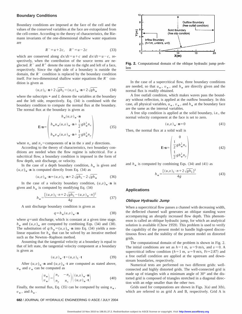
The computational domain of the problem is shown in FigThe initial conditions are set ash51 m, u59 m/s, andv50. Asupercritical inflow condition (h51 m, u59 m/s, Fr52.87! anda free outfall condition are applied at the upstream and dstream boundaries, respectively.

Numerical tests are performed on two different grids: wconnected and highly distorted grids. The well-connected gmade up of triangles with a minimum angle of 30° and thetorted grid is composed of triangles stretched in a diagonal dtion with an edge smaller than the other two.

Grids used for computations are shown in Figs. 3~a! and 3~b!,

Fig. 2. Computational domain of the oblique hydraulic jump prlem

which are referred to as grid A and B, respectively. Grid A is


1,831ut byod,’’

was

tedd A.ithd 5per-

om-om-the

m/s,tions

thee 1,

t nu-

thet. As-reeratesfons

con-rid.od’’om-ch

n of acy isodeland

-meri-odellity ofng ac-veryws.

iouset al.meri-lties

l

made up of 1,880 elements and 1,000 nodes and grid Belements and 1,000 nodes. Computations were carried ousing a first-order and second-order scheme with the ‘‘minmthe ‘‘superbee’’ limiters~Anastasiou and Chan 1997!, and thepresent model. The model was run until a steady statereached.

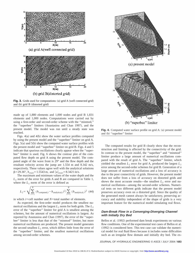
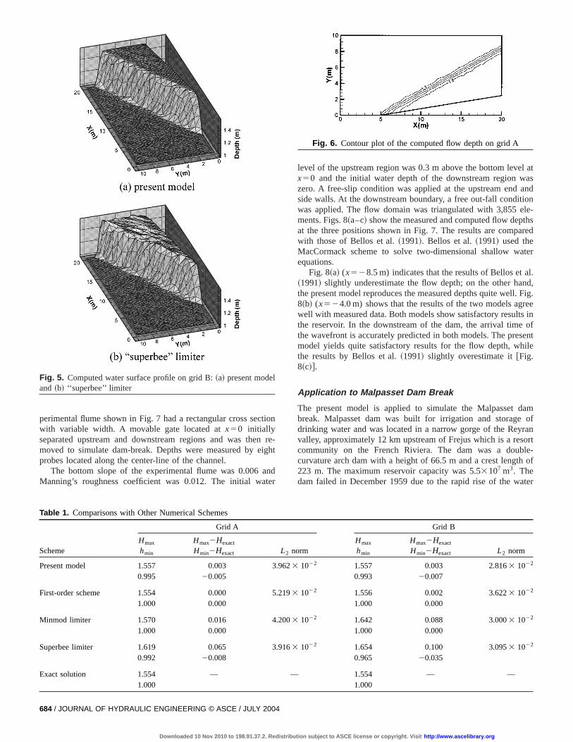
Figs. 4~a! and 4~b! show the water surface profiles compuby using the present model and the ‘‘superbee’’ limiter on griFigs. 5~a! and 5~b! show the computed water surface profiles wthe present model and ‘‘superbee’’ limiter on grid B. Figs. 4 anindicate that spurious oscillations clearly appear when the ‘‘subee’’ limiter is used. Fig. 6 shows the contour plot of the cputed flow depth on grid A using the present model. The cputed angle of the wave front is 29° and the flow depth andresultant velocity across the jump are 1.554 m and 8.342respectively. These values agree well with the analytical solub529.36°,hexact51.5543 m, anduuuexact58.3421 m/s.

The maximum and minimum values of the water depth andL2 norm of the error for grids A and B are compared in Tablwhere theL2 norm of the error is defined as

L25A(i 51

N

~hcomputed,i2hanalytical,i !2/(

i 51

N

~hanalytical,i !2 (44)

in which i5cell number andN5total number of elements.As expected, the first-order model produces the smalles

merical oscillations and the largestL2 norm for both grids. TheL2

error of the ‘‘superbee’’ limiter for grid A is smallest amongschemes, but the amount of numerical oscillations is largesreported by Anastasiou and Chan~1997!, the error of the ‘‘superbee’’ limiter is less than that of the ‘‘minmod’’ limiter, but monumerical oscillations are produced. The present model genthe second smallestL2 error, which differs little from the error othe ‘‘superbee’’ limiter, and the smallest numerical oscillati

Fig. 3. Grids used for computations:~a! grid A ~well connected grid!and ~b! grid B ~distorted grid!

among second-order schemes.

JO


The computed results for grid B clearly show that the restruction and limiting is affected by the connectivity of the gIn contrast to the present model, the ‘‘superbee’’ and ‘‘minmlimiter produce a large amount of numerical oscillations cpared with the result of grid A. The ‘‘superbee’’ limiter, whiyielded the smallestL2 error for grid A, produced the largestL2

error among the second-order schemes for grid B. Generatiolarge amount of numerical oscillations and a loss of accuradue to the poor connectivity of grids. However, the present mdoes not suffer from a loss of accuracy on distorted gridsshows the most accurate results—the smallestL2 error and numerical oscillations—among the second-order schemes. Nucal tests on two different grids indicate that the present mpreserves accuracy even on a distorted grid. Since the quathe generated mesh cannot always be satisfactory, preservicuracy and stability independent of the shape of grids is aimportant feature for the numerical model simulating real flo

Dam-Break Flow in a Converging-Diverging Channelwith Initially Dry Bed

Bellos et al.~1992! performed dam break experiments on varflow conditions. One of the experimental test cases of Bellos~1992! is considered here. This test case can validate the nucal model for real fluid flows because it includes some difficu

Fig. 4. Computed water surface profile on grid A:~a! present modeand ~b! ‘‘superbee’’ limiter

such as an irregular flow domain and initially dry bed. The ex-



ction

en reeight

andater

el atwasand

itionele-pthspared

ater

al.and,ll. Fig.greelts ine ofesenthile

dame ofyransortble-th of

ater

l

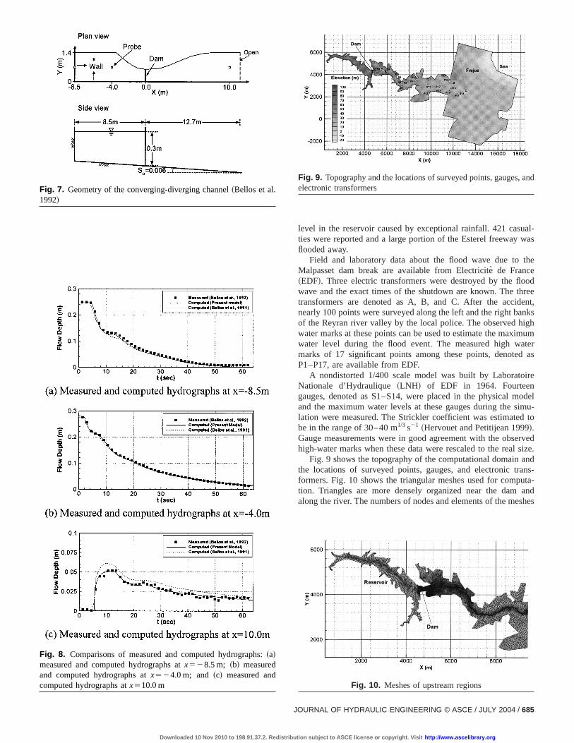
perimental flume shown in Fig. 7 had a rectangular cross sewith variable width. A movable gate located atx50 initiallyseparated upstream and downstream regions and was thmoved to simulate dam-break. Depths were measured byprobes located along the center-line of the channel.

The bottom slope of the experimental flume was 0.006Manning’s roughness coefficient was 0.012. The initial w

Fig. 5. Computed water surface profile on grid B:~a! present modeand ~b! ‘‘superbee’’ limiter

Table 1. Comparisons with Other Numerical Schemes

Scheme

Grid A

Hmax

hmin

Hmax2Hexact

Hmin2Hexact

Present model 1.557 0.0030.995 20.005

First-order scheme 1.554 0.0001.000 0.000

Minmod limiter 1.570 0.0161.000 0.000

Superbee limiter 1.619 0.0650.992 20.008

Exact solution 1.554 —1.000



-

level of the upstream region was 0.3 m above the bottom levx50 and the initial water depth of the downstream regionzero. A free-slip condition was applied at the upstream endside walls. At the downstream boundary, a free out-fall condwas applied. The flow domain was triangulated with 3,855ments. Figs. 8~a–c! show the measured and computed flow deat the three positions shown in Fig. 7. The results are comwith those of Bellos et al.~1991!. Bellos et al.~1991! used theMacCormack scheme to solve two-dimensional shallow wequations.

Fig. 8~a! (x528.5 m) indicates that the results of Bellos et~1991! slightly underestimate the flow depth; on the other hthe present model reproduces the measured depths quite we8~b! (x524.0 m) shows that the results of the two models awell with measured data. Both models show satisfactory resuthe reservoir. In the downstream of the dam, the arrival timthe wavefront is accurately predicted in both models. The prmodel yields quite satisfactory results for the flow depth, wthe results by Bellos et al.~1991! slightly overestimate [email protected]~c!#.

Application to Malpasset Dam Break

The present model is applied to simulate the Malpassetbreak. Malpasset dam was built for irrigation and storagdrinking water and was located in a narrow gorge of the Revalley, approximately 12 km upstream of Frejus which is a recommunity on the French Riviera. The dam was a doucurvature arch dam with a height of 66.5 m and a crest leng223 m. The maximum reservoir capacity was 5.53107 m3. Thedam failed in December 1959 due to the rapid rise of the w

Fig. 6. Contour plot of the computed flow depth on grid A

Grid B

rmHmax

hmin

Hmax2Hexact

Hmin2Hexact L2 norm

21022 1.557 0.003 2.8163 1022

0.993 20.007

91022 1.556 0.002 3.6223 1022

1.000 0.000

1022 1.642 0.088 3.0003 1022

1.000 0.000

1022 1.654 0.100 3.0953 1022

0.965 20.035

1.554 — —1.000

L2 no

3.963

5.213

4.2003

3.9163

—


sual-was

the

oodthreedent,ankshighimumaterd as

oirenmodelsimu-ed to

servedl size.and

trans-puta-

andeshes

.

s:dd

, and

JO


level in the reservoir caused by exceptional rainfall. 421 caties were reported and a large portion of the Esterel freewayflooded away.

Field and laboratory data about the flood wave due toMalpasset dam break are available from Electricite` de France~EDF!. Three electric transformers were destroyed by the flwave and the exact times of the shutdown are known. Thetransformers are denoted as A, B, and C. After the accinearly 100 points were surveyed along the left and the right bof the Reyran river valley by the local police. The observedwater marks at these points can be used to estimate the maxwater level during the flood event. The measured high wmarks of 17 significant points among these points, denoteP1–P17, are available from EDF.

A nondistorted 1/400 scale model was built by LaboratNationale d’Hydraulique~LNH! of EDF in 1964. Fourteegauges, denoted as S1–S14, were placed in the physicaland the maximum water levels at these gauges during thelation were measured. The Strickler coefficient was estimatbe in the range of 30–40 m1/3s21 ~Hervouet and Petitijean 1999!.Gauge measurements were in good agreement with the obhigh-water marks when these data were rescaled to the rea

Fig. 9 shows the topography of the computational domainthe locations of surveyed points, gauges, and electronicformers. Fig. 10 shows the triangular meshes used for comtion. Triangles are more densely organized near the damalong the river. The numbers of nodes and elements of the m

Fig. 9. Topography and the locations of surveyed points, gaugeselectronic transformers

Fig. 10. Meshes of upstream regions

Fig. 7. Geometry of the converging-diverging channel~Bellos et al1992!

Fig. 8. Comparisons of measured and computed hydrograph~a!measured and computed hydrographs atx528.5 m; ~b! measureand computed hydrographs atx524.0 m; and~c! measured ancomputed hydrographs atx510.0 m



. The,000-

sead theoints.ts of

atir isreamrougho beth inaffecton. Ad thes the

le run

nts is

istri--

f theyed.

dry.lly in

reaksent

es de-DF.by

teral

of thel timeto ben isodtwo

pro-com-

ithedata.th theand

e

s

ers

used for the computation are 34,849 and 67,719, respectivelybottom elevation of the valley was obtained from the 1:20ancient IGN~Institut Geographique National! maps. The elevations range from220 m below sea level to 100 m abovelevel. The number of digitized points amounted to 13,541 anbottom elevation at each node was interpolated from these p

The dam is considered as a straight line between the poin(x,y) coordinates being~4,701.18 m, 4,143.41 m! and ~4,656.5m, 4,392.10 m!, and instantaneous removal of the entire damthe timet50 is assumed. The initial water level in the reservo100 m above sea level which is equal to zero. In the downstof the dam, the bottom is set to dry because the discharge ththe outlet gate is unknown and its quantity is considered tsmall compared with that of the flood wave. The water depthe sea is also removed for convenience since it does notthe solution at surveyed points and gauges during computatisolid boundary condition is imposed along all boundaries anManning roughness coefficient is set to 0.033, which equalStrickler coefficient of 30 m1/3s21.

The computation was run until the timet53,000 s. The modewas run on a PC with a Pentium 4 2.4 Ghz processor and thtime of the test case was about 7 h 15 min. The run time isconsidered not excessive given that the number of elemeapproximately 70,000.

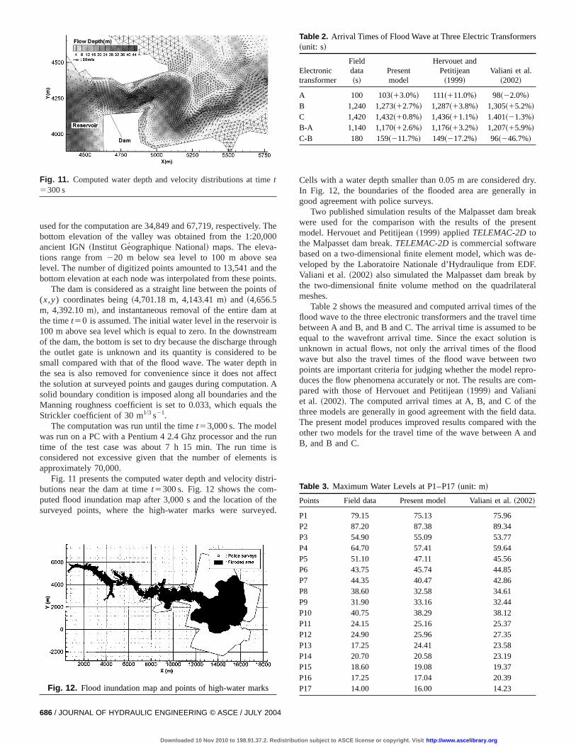
Fig. 11 presents the computed water depth and velocity dbutions near the dam at timet5300 s. Fig. 12 shows the computed flood inundation map after 3,000 s and the location osurveyed points, where the high-water marks were surve

Fig. 11. Computed water depth and velocity distributions at timt5300 s

Fig. 12. Flood inundation map and points of high-water mark



Cells with a water depth smaller than 0.05 m are consideredIn Fig. 12, the boundaries of the flooded area are generagood agreement with police surveys.

Two published simulation results of the Malpasset dam bwere used for the comparison with the results of the premodel. Hervouet and Petitijean~1999! appliedTELEMAC-2Dtothe Malpasset dam break.TELEMAC-2Dis commercial softwarbased on a two-dimensional finite element model, which waveloped by the Laboratoire Nationale d’Hydraulique from EValiani et al. ~2002! also simulated the Malpasset dam breakthe two-dimensional finite volume method on the quadrilameshes.

Table 2 shows the measured and computed arrival timesflood wave to the three electronic transformers and the travebetween A and B, and B and C. The arrival time is assumedequal to the wavefront arrival time. Since the exact solutiounknown in actual flows, not only the arrival times of the flowave but also the travel times of the flood wave betweenpoints are important criteria for judging whether the model reduces the flow phenomena accurately or not. The results arepared with those of Hervouet and Petitijean~1999! and Valianet al. ~2002!. The computed arrival times at A, B, and C ofthree models are generally in good agreement with the fieldThe present model produces improved results compared wiother two models for the travel time of the wave between AB, and B and C.

Table 2. Arrival Times of Flood Wave at Three Electric Transform~unit: s!

Electronictransformer

Fielddata~s!

Presentmodel

Hervouet andPetitijean~1999!

Valiani et al.~2002!

A 100 103~13.0%! 111~111.0%! 98~22.0%!

B 1,240 1,273~12.7%! 1,287~13.8%! 1,305~15.2%!

C 1,420 1,432~10.8%! 1,436~11.1%! 1.401~21.3%!

B-A 1,140 1,170~12.6%! 1,176~13.2%! 1,207~15.9%!

C-B 180 159~211.7%! 149~217.2%! 96~246.7%!

Table 3. Maximum Water Levels at P1–P17~unit: m!

Points Field data Present model Valiani et al.~2002!

P1 79.15 75.13 75.96P2 87.20 87.38 89.34P3 54.90 55.09 53.77P4 64.70 57.41 59.64P5 51.10 47.11 45.56P6 43.75 45.74 44.85P7 44.35 40.47 42.86P8 38.60 32.58 34.61P9 31.90 33.16 32.44P10 40.75 38.29 38.12P11 24.15 25.16 25.37P12 24.90 25.96 27.35P13 17.25 24.41 23.58P14 20.70 20.58 23.19P15 18.60 19.08 19.37P16 17.25 17.04 20.39P17 14.00 16.00 14.23


sultsfor

ent is

umthe

ts

beenwet

han-lvinglver.ionalulti-

racy.n on

dis-odelk testree-com-mmentThis

s usedesent

allowith

theirhankthe

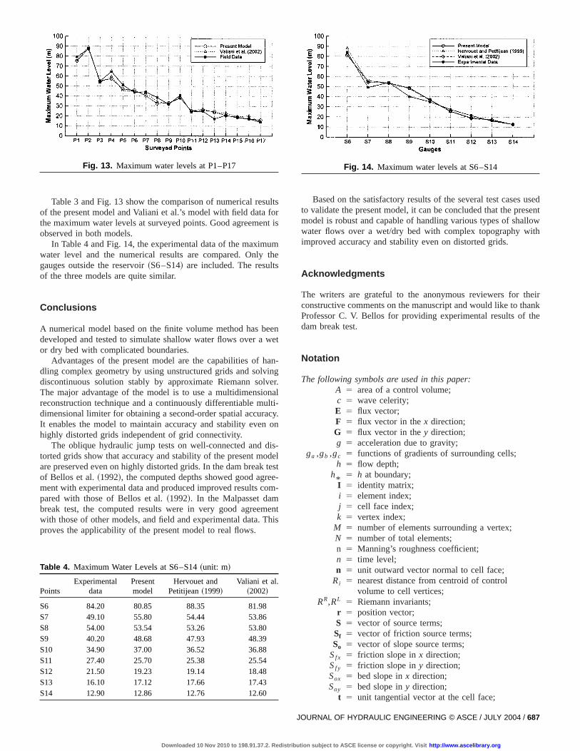
Table 3 and Fig. 13 show the comparison of numerical reof the present model and Valiani et al.’s model with field datathe maximum water levels at surveyed points. Good agreemobserved in both models.

In Table 4 and Fig. 14, the experimental data of the maximwater level and the numerical results are compared. Onlygauges outside the reservoir~S6–S14! are included. The resulof the three models are quite similar.

Conclusions

A numerical model based on the finite volume method hasdeveloped and tested to simulate shallow water flows over aor dry bed with complicated boundaries.

Advantages of the present model are the capabilities ofdling complex geometry by using unstructured grids and sodiscontinuous solution stably by approximate Riemann soThe major advantage of the model is to use a multidimensreconstruction technique and a continuously differentiable mdimensional limiter for obtaining a second-order spatial accuIt enables the model to maintain accuracy and stability evehighly distorted grids independent of grid connectivity.

The oblique hydraulic jump tests on well-connected andtorted grids show that accuracy and stability of the present mare preserved even on highly distorted grids. In the dam breaof Bellos et al.~1992!, the computed depths showed good agment with experimental data and produced improved resultspared with those of Bellos et al.~1992!. In the Malpasset dabreak test, the computed results were in very good agreewith those of other models, and field and experimental data.proves the applicability of the present model to real flows.

Fig. 13. Maximum water levels at P1–P17

Table 4. Maximum Water Levels at S6–S14~unit: m!

PointsExperimental

dataPresentmodel

Hervouet andPetitijean~1999!

Valiani et al.~2002!

S6 84.20 80.85 88.35 81.98S7 49.10 55.80 54.44 53.86S8 54.00 53.54 53.26 53.80S9 40.20 48.68 47.93 48.39S10 34.90 37.00 36.52 36.88S11 27.40 25.70 25.38 25.54S12 21.50 19.23 19.14 18.48S13 16.10 17.12 17.66 17.43S14 12.90 12.86 12.76 12.60

JO


Based on the satisfactory results of the several test caseto validate the present model, it can be concluded that the prmodel is robust and capable of handling various types of shwater flows over a wet/dry bed with complex topography wimproved accuracy and stability even on distorted grids.

Acknowledgments

The writers are grateful to the anonymous reviewers forconstructive comments on the manuscript and would like to tProfessor C. V. Bellos for providing experimental results ofdam break test.

Notation

The following symbols are used in this paper:A 5 area of a control volume;c 5 wave celerity;E 5 flux vector;F 5 flux vector in thex direction;G 5 flux vector in they direction;g 5 acceleration due to gravity;

ga ,gb ,gc 5 functions of gradients of surrounding cells;h 5 flow depth;

h* 5 h at boundary;I 5 identity matrix;i 5 element index;j 5 cell face index;k 5 vertex index;

M 5 number of elements surrounding a vertex;N 5 number of total elements;n 5 Manning’s roughness coefficient;n 5 time level;n 5 unit outward vector normal to cell face;

Ri 5 nearest distance from centroid of controlvolume to cell vertices;

RR,RL 5 Riemann invariants;r 5 position vector;S 5 vector of source terms;Sf 5 vector of friction source terms;So 5 vector of slope source terms;

Sf x 5 friction slope inx direction;Sf y 5 friction slope iny direction;Sox 5 bed slope inx direction;Soy 5 bed slope iny direction;

Fig. 14. Maximum water levels at S6–S14

t 5 unit tangential vector at the cell face;



-

-ns.’’

trian-

t.

-ws.’’

s-

-

-.,

r.’’

el

n-

and

ingc.

etme

-allow

. Y.for

t 5 temporal coordinate;U 5 vector of the conserved variables;u 5 vertically averaged velocities inx direction;

u* 5 u at boundary;v 5 vertically averaged velocities iny direction;

v* 5 v at boundary;x,y 5 orthogonal Cartesian coordinates;

z 5 bottom elevation;G 5 boundary of a control volume;D 5 finite difference operator;¹ 5 nabla operator;

va ,vb ,vc 5 weights used to limit gradient of solution.

References

Akanbi, A. A., and Katopodes, N. D.~1988!. ‘‘Model for flood propagation on initially dry land.’’ J. Hydraul. Eng.,114~7!, 689–706.

Alcrudo, F., and Garcia-Navarro, P.~1993!. ‘‘A high-resolution Godunovtype scheme in finite volumes for the 2D shallow water equatioInt. J. Numer. Methods Fluids,16, 489–505.

Anastasiou, K., and Chan, C. T.~1997!. ‘‘Solution of the 2D shallowwater equations using the finite volume method on unstructuredgular meshes.’’Int. J. Numer. Methods Fluids,24, 1225–1245.

Bellos, C. V., Soulis, J. V., and Sakkas, J. G.~1991!. ‘‘Computation oftwo-dimensional dambreak induced flows.’’Adv. Water Resour.,30,14~1! ~31–41!.

Bellos, C. V., Soulis, J. V., and Sakkas, J. G.~1992!. ‘‘Experimentalinvestigation of two-dimensional dam-break induced flows.’’J. Hy-draul. Res.,30~1!, 47–63.

Chow, V. T. ~1959!. Open-channel hydraulics, McGraw-Hill, New York.Fennema, R. J., and Chaudhry, M. H.~1990!. ‘‘Explicit method for 2-D

transient free-surface flows.’’J. Hydraul. Eng.,116~8!, 1013–1034.Garcia, R., and Kahawita, R. A.~1986!. ‘‘Numerical solution of the S

Venant equations with the MacCormack finite-difference scheme.’’



Int. J. Numer. Methods Fluids,6, 259–274.Harten, A., Lax, P. D., and van Leer, B.~1983!. ‘‘On upstream differenc

ing and Godunov-type schemes for hyperbolic conservation laSIAM Rev.,25~1!, 35–61.

Hervouet, J.-M., and Petitijean, A.~1999!. ‘‘Malpasset dam-break reviited with two-dimensional computations.’’J. Hydraul. Res.,37~6!,777–788.

Holmes, D. G., and Connel, S. D.~1989!. ‘‘Solution of the 2D NavierStokes equations on unstructured adaptive grids.’’Proc., AIAA 9thCFD Conf., AIAA Paper 89-1932.

Hubbard, M. E.~1999!. ‘‘Multidimensional slope limiters for MUSCLtype finite volume schemes on unstructured grids.’’J. Comput. Phys155, 54–74.

Jawahar, P., and Kamath, H.~2000!. ‘‘A high-resolution procedure foEuler and Navier-Stokes computations on unstructured gridsJ.Comput. Phys.,164, 165–203.

Molls, T., and Chaudhry, M. H.~1995!. ‘‘Depth-averaged open channflow model.’’ J. Hydraul. Eng.,121~6!, 453–465.

Shu, C. W., and Osher, S.~1988!. ‘‘Efficient implementation of essetially non-oscillatory shock capturing schemes.’’J. Comput. Phys.,77,439–471.

Sleigh, P. A., Gaskell, P. H., Berzins, M., and Wright, N. G.~1998!. ‘‘Anunstructured finite-volume algorithm for predicting flow in riversestuaries.’’Comput. Fluids,27~4!, 479–508.

Toro, E. ~1992!. ‘‘Riemann problems and the WAF method for solvthe two-dimensional shallow water equations.’’Philos. Trans. R. SoLondon, Ser. A,338, 43–68.

Valiani, A., Caleffi, V., and Zanni, A.~2002!. ‘‘Case Study: Malpassdam-break simulation using a two-dimensional finite volumethod.’’J. Hydraul. Eng.,128~5!, 460–472.

Wang, J.-W., and Liu, R.-X.~2000!. ‘‘A comparative study of finite volume methods on unstructured meshes for simulation of 2D shwater wave problems.’’Math. Comput. Simul.,53, 171–184.

Zhao, D. H., Shen, H. W., Tabios, III, G. Q., Lai, J. S., and Tan, W~1994!. ‘‘Finite-volume two-dimensional unsteady-flow model
river basins.’’J. Hydraul. Eng.,120~7!, 863–883.

Finite Volume Model for Two-Dimensional Shallow …Finite Volume Model for Two-Dimensional Shallow...

Documents

Transcript of Finite Volume Model for Two-Dimensional Shallow …Finite Volume Model for Two-Dimensional Shallow...