THREE-DIMENSIONAL FINITE STRIP ANALYSIS OF ELASTIC SOLIDS

M.S. Cheung and M.Y.T. Chan Public Works Canada

SUMMARY

Three-dimensional (3-D) finite strips are formulated by combining finite element shape functions with beam eigenfunctions. Because of the orthogonality of the beam functions, three-dimensional problems are reduced to a series of two-dimensional problems, often with stiffness matrices of very narrow bandwidth. These require considerably less computer memory and computation time to solve. Isoparametric and high order finite element shape functions are used in the formulation of the 3-D finite strips. Numerical examples such as the static and free vibration analyses of simply supported thick plates are presented. Results are compared with existing solutions. Good agreements are obtained in all cases. Potential applications of the 3-D finite strips include the static and dynamic analyses of voided slabs, thick box girders and axisymmetric thick-walled shell structures.

INTRODUCTION

Although the finite element method is at present the most powerful and versatile numerical approach for structural analysis, the computing cost can often be very high. This is particularly true in the case of three- dimensional structural analyses. In an attempt to reduce the computational requirements of the finite element method, researchers have developed the finite strip technique (ref.11, a semi-analytical method that couples simple polynomial expressions for one or two directions with beam eigenfunction series for the other directions. This reduces a two-dimensional problem to one dimension, and a three-dimensional problem to two dimensions. Furthermore, because of the orthogonal properties of the eigenfunction series, the terms of the series may become uncoupled depending on the type of boundary conditions, and the stiffness matrices of each term can be formed, assembled and solved separately, resulting in a substantial reduction in computing costs. The method.is suited for the analysis of structures having regular geometric plans and simple boundary conditions, and has been successfully applied to the static and the dynamic analyses of slabs, folded plate structures and box-girder bridges (ref. I).

In this study, 3-D finite strips are formulated in two ways, one by coupling isoparametric quadrilateral and triangular plane-stress finite element shape functions with beam eigenfunctions, and the second by coupling high order quadr.ilateral plane-stress finite element shape functions with beam eigenfunctions. The stiffness, mass and load matrices are derived following standard finite element procedures. Three-dimensional elasticity

153

https://ntrs.nasa.gov/search.jsp?R=19790002289 2018-07-15T11:34:32+00:00Z

constitutive equations are used in the derivation of the various stiffness matrices. Applications of the 3-D finite strips to some prismatic solids such as thick plates are described. Numerical integration -using Legendre- Gauss or Radau-Gauss quadratures was employed in the derivations.

SYMBOLS

al’ a2, etc.

a A

[Bl [cl [Dl {F) ,(F)

{gl h

L,’ L2’ L3

[Kl , [RI [Ml , [fll N n

{PI P

(41 V

us VY w

x9 Y, =

lengths of sides of a quadrilateral span of 3-D finite strips surface area of 3-D finite strips matrix relating strains to displacement components matrix containing finite strip displacement functions material constant matrix

individual and assembled consistent load vectors vector containing distributed body forces thickness of plate triangular area co-ordinates individual and assembled stiffness matrices individual and assembled consistent mass matrices finite element shape functions

number of nodes in finite elements vector containing concentrated nodal forces point in 5 - n space or a concentrated point

load vector containing distributed surface forces

volume of 3-D finite strip displacement components in the x, y and z directions Cartesian co-ordinates distance along lines of equal n (equation 8) indiv.i.dual and assembled nodal displacement vectors curvilinear co-ordinates finite element rotational degree of freedom &W/ax )

Si 3-D finite strip rotational degree of freedom =(aw/aX& mass density

circular natural frequencies

154

w XY

!d XZ

finite element skew symmetric rotational degree of freedom dadax - aday)/

3-D finite strip skew symmetric rotational degree of freedom dadax - au/as2

ISOPARAMETRIC 3-D FINITE STRIPS

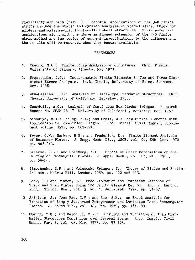
A family of 3-D isoparametric quadrilateral and triangular finite strips can be developed by using the plane-stress isoparametric finite element shape functions reported by Ergatoudis (ref. 2). Considering only simply supported situations in which u=w=av/ay=O at the ends, a suitable set of displacement functions for a 3-D strip of span a (fig. 1) is

OD n u = c C N u i im sin=

m=l i=l a

00

v = c c” Nivimcosy m=l i=l

(1)

Q) n w= c C N w i im sin= a

m=l i=l

The x and z co-ordinates of the isoparametric section are defined as

x q ; Nx ii i=l n

z = C Nizi (2) i=l

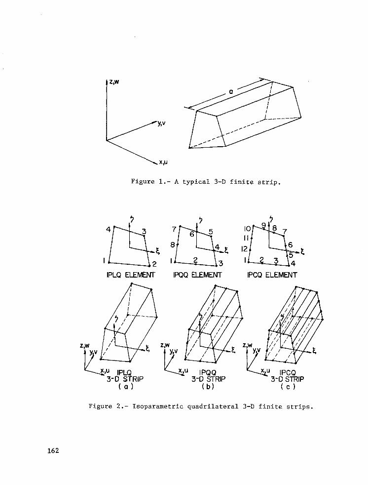
The most simple isoparametric quadrilateral is the four node IPLQ quardi- laterial (ref. 2) which has linearly varying displacements (fig. 2a). The shape functions for this finite element are simply

Ni q +, (1 + SSi) (1 + W-Q) (3)

Other more sophisticated isoparametric quadrilateral elements of the same family include the eight node IPQQ quadrilateral (ref. 2) whose dis- placements vary quadratically (fig. 2b), and the twelve node IPCQ quadrilateral (ref. 2) with cubically varying displacements (fig. 2~).

155

For the Isoparametric triangular finite elements, the shape functions are most conveniently expressed in terms of the area co-ordinates Ll, L2 and

L3. The first element of the series is the three node IPCST constant strain

triangle (fig. 3a) whose shape functions are simply the area co-ordinates (ref. 2). Thus,

N1 q L,, N2 q L2, N3

= L3 (4)

Using a recurrence formula (ref. 21, more refined triangular elements such as the six node IPLST linear strain triangle (fig. 3b) and the ten node IPQST quadratic strain triangle (fig. 3c) can be formulated.

Although in theory more refined elements can be derived by introducing additional nodes, such elements are often of limited practical use since they usually result in stiffness matrices having very large bandwidths.

HIGH ORDER QUADRILATERAL 3-D FINITE STRIPS

Because of its linearly varying displacements, the accuracy of the IPLQ 3-D finite strip is usually very limited. The strip could be refined by adding extra nodes as was done in the last section. However, such a procedure is not always desirable, since the bandwidths of the stiffness matrices are increased. The alternative, and probably most effective, approach is to introduce additional degrees of freedom at the nodes. Two high order plane stress quadrilateral finite elements were selected from the published literature for this purpose.

The first element is the QCC3 in-plane quadrilateral with displacements u, v and the skew symmetric rotations

w =- ’ (g - $) XY 2

(5)

as degrees of freedom (fig. 4a). This element was derived by Abu-Ghazaleh (ref. 3) and subsequently used by Scordelis (ref. 4) to analyze box-girder bridges.

Using strip with

w q xz

as degrees of freedom is formulated (fig. 4a). Considering only simply supported cases, the displacement functions of the finite strip can be written as

the shape function of this finite element, a high order 3-D finite u, VY w and the skew symmetric rotations

(6)

co 4 u = c C [N +N w

m=l i=l li Uim 2i xziml sin y

156

;r -

i ,, 1 .I

‘, / I

m=l i=l

co ; IN !!Ex

w= c Ii Wim + N3i~xziml sin a

(7)

m=l i=l where the shape functions N ,i, .N2i and N3i are the same as those used for the finite element in reference 3.

The other high order element selected is the plane stress QLC3 element developed by Sisodiya et al.(ref. 5). The nodal parameters of the element are 161 = [u, v, eZIT, i with ezi=(av/ax~)i where x

5 is a distance along lines

equal n (fig. 4b); and at a general point P

(8)

of

where a 1 and a3 are the lengths of opposite sides of a quadrilateral (fig. 4b).

Adopting the shape function of the element for the 3-D finite strip, the displacement functions of a simply supported 3-D strip can be expressed as

cm u=c

m=l

co v=c

m=l

co w q c

m=l

where 8 yi = and N 3i are

(9)

4 .?I N

i=l li "im sin=

a

4 1 N

i=l li 'im c0s-f a

4 C [N2i wim + N3i eyim] sin y

i=l

cadax, 1 ad xs ,i is as defined before. The functions Nli, N2i

identical to those presented in reference 5.

STIFFNESS, MASS AND LOAD MATRICES

The stiffness and load matrices can be derived through the minimization of the total potential energy, a standard finite element procedure that leads to the familar expression

157

[ti (6) - tF1 = 0 (IO)

in which [Kl is the stiffness matrix, {S) the unknown nodal displacement vector and (F) the consistent load vector. the stiffness matrix [Kl is

A typical submatrix [Kijj of

fKijl = JrBl $Dl [Bl .dV J

(II)

where [Bl is the so-called strain matrix that relates the strains to the displacement components and [Dl is the elasticity matrix for the material which can 'be isotropic or orthotropic. is

A typical submatrix {Fi} of IF}

iFi = {Pi) + j$lT{qjdA + .&~T~g~dV (I‘?)

where [Gil contains the nodal displacement functions and the force terms

represent concentrated, surface and body forces.

Using the displacement functions defined in the previous sections, equation (II) would become

(13)

Because of the orthogonality of the series used, it can be shown that for llfm

2 JJ!i3,1i[3: :13j] ,jxdz for 9, = m (14)

l.e., the series terms are uncoupled and off-diagonal submatrices in the stiffness matrix are null matrices.

To obtain the consistent load vector for the 3-D strips, the external applied loads are expressed in terms of series similar to those used for the displacement functions and substituted into the appropriate integrals in equation (12). Details of the derivation of the load terms can be found in reference 1.

The formula for deriving the consistent mass matrix is quite standard, and is

[Ml = Io[CITrCldV (15)

where [Ml is the consistent mass matrix and p is the mass density of the material.

As the displacement functions are either defined in terms of the cur- vilinear co-ordinates 5 and n or area co-ordinates L,, L2 and L 3, it is necessary to rewrite the derivatives and integrals of the displacements with respect to the local co-ordinate system. This is a fairly straightforward matter involving the determination of the Jacobian matrix (ref. 2).

158

Once the individual finite strip stiffness, mass and load matrices are formulated, they can be assembled in the usual manner to form the -static problem of

riz1 (8) - {PI = 0

or the free vibration problem of

CL81 - flJ2 ml > (8) = 0

(16)

(17)

where [El , [RI , (!?I and (8) are respectively the assembled stiffness, mass, load and displacement matrices, and w is the circular frequency of free vibration.

ILLUSTRATIVE EXAMPLES

Static and free vibration analyses were carried out for the simply supported thick, square plate shown in fig. 5. The central deflections due to uniformly distributed load and a central point load are shown in tables 1 and 2. The values shown were obtained with ten series terms. Comparing the present results with existing finite element solutions (ref. 6) and closed form solutions (ref. 7) as well as the classical thin plate theory (ref. 81, it can be seen that the agreement is good. By doubling the number of series terms in a number of runs, it-was found that the displace- ment values remained unchanged. The first three lowest flexural frequencies for a simply supported square plate with a thickness vs. span ratio of 0.2 are tabulated in table 3. Excellent agreement 'between the present frequencies and those obtained from finite element (ref. 9) and closed form (ref. 10) solutions can be seen, while the thin plate theory tends to overestimate the frequencies. The results in tables 1-3 indicate that the effects of thickness-shear deformation and rotary inertia can be accurately predicted by the present 3-D finite strip formulation.

CONCLUDING REMARKS

Three-dimensional (3-D) simply supported finite strips with quadri- lateral and triangular cross sections have been formulated using isopara- metric and high order finite element shape functions and beam eigenfunctions. In general, the accuracies of both the isoparametric and high order 3-D strips can be considered good since reasonably good results can be achieved even with a relatively coarse mesh.

Three-dimensional finite strips with other than simply supported boundaries can be derived by employing the appropriate beam eigenfunctions to match the boundary conditions. Curved, and circular 3-D strips can be developed by using a cylindrical co-ordinate formulation. Continuous structures can be analyzed either by coupling the finite element shape functions with eigenfunctions of continuous beams (ref. II); or by using a finite strip

159

flexibility approach (ref. I). Potential applications of the 3-D finite strips include the static and dynamic analyses of voided slabs, thick box girders and axisymmetric thick-walled shell structures. These potential applications along with the above mentioned extension of the 3-D finite strip method are the topics of current investigations by the authors; and the results will be reported when they become available.

1.

2.

3.

4.

5.

6.

7.

8.

9.

10.

11.

REFERENCES

Cheung, M.S.: Finite Strip Analysis of Structures. Ph.D. Thesis, University of Calgary, Alberta, May 1971.

Ergatoudis, J.G.: Isoparametric Finite Elements in Two and Three Dimen- sional Stress Analysis. Ph.D., Thesis, University of Wales, Swansea, Oct. 1968.

Abu-Gazaleh, B.N.: Analysis of Plate-Type Prismatic Structures. Ph.D. Thesis, University of Calfornia, Berkeley, 1965.

Scordelis, A.C.: Analysis of Continuous Box-Girder Bridges. Research Report No. SESM 66-17, University of California, Berkeley, Oct. 1967.

Sisodiya, R.G.; Cheung, Y.K.; and Ghali, A.: New Finite Elements with Application to Box-Girder Bridges. Proc. Instit. Civil Engrs., Supple- ment Volume, 1972, pp. 207-224.

Pryor, C.W.; Barker, R.M.; and Frederick, D.: Finite Element Analysis of Reissner Plates. J. Engg. Mech. Div., ASCE, vol. 96, EM6, Dec. 1970, pp. 963-983.

Salerno, V.L.; and Goldberg, N.A.: Effect of Shear Deformation on the Bending of Rectangular Plates. J. Appl. Mech., vol. 27, Mar. 1960, pp. 54-58.

Timoshenko, S.P.; and Woinowsky-Krieger, S.: Theory of Plates and Shells. 2nd edn., McGraw-Hill, London, 1959, pp. 120 and 143.

Rock, T.; and Hinton, E.: Free Vibration and Transient Response of Thick and Thin Plates Using the Finite Element Method. Int. J. Earthq. ha. Struct. Dyn., vol. 3, No. 1, Jul.-Sept. 1974, pp. 51-63.

Srinivas, S.; Joga Rao, C.V.; and Rao, A.K.: An Exact Analysis for Vibration of Simply-Supported Homogeneous and Laminated Thick Rectangular Plates. J. Sound Vib., vol. 12, Feb. 1970, pp. 187-199.

Cheung, Y.K.; and Delcourt, C.R.: Buckling and Vibration of Thin Flat- Walled Structures Continuous over Several Spans. Proc. Instit. Civil Enars. Part 2. vol. 63. Mar. 1977. DD. 93-103.

160

TABLE 1 COMPARISON OF CENTRAL DEFLECTIONS FOR SIMPLY SUPPORTED PLATES UNDER UDL

IPLQ IPQQ IPCQ IPCST IPLST IPQST QCC3 QLC3 REF. 6 REF. 7 REF. 8

- . _--. _ __i_-- - h/a=0.05 h/a=O.l h/a=0.2 h/a=0.25

j- --.-.-- - -_ 3692.1 463.4 64.1 35.4 3694.0 482.1 65.5 36.3 3704.2 487.2 67.1 36.4 3681.1 462.1 63.2 34.2 3688.5 465.2 64.8 36.3 3701.1 471.3 66.1 36.5 3683.1 465.4 64.3 35.5 3686.5 465.1 64.5 35.8 3575.2 461.2 64.8 35.9 3588.8 463.2 65.2 36.2 3549.6 443.7 55.5 28.4

TABLE 2 COMPARISON OF CENTRAL DEFLECTIONS FOR SIMPLY SUPPORTED PLATES UNDER POINT LOAD

IPLQ IPQQ IPCQ IPCST IPLST IPQST QCC3 QLC3 REF. 6 REF. 8

h/a=0.05 h/a=O.l h/a=0.2 h/a=0.25 105.98 - 13.97 2.24 1.39 106.52 14.47 2.31 1.43 106.71 14.87 2.36 1.49 104.92 13.88 2.27 1.39 106.16 14.32 2.29 1.42 106.89 14.77 2.32 1.48 106.11 14.12 2.28 1.41 106.31 14.16 2.30 1.41 106.49 14.77 2.46 1.47 101.34 12.67 1.58 0.81

TABLE 3 COMPARISON OF CIRCULAR FREQUENCIES OF A SIMPLY SUPPORTED THICK PLATE (h/a=0.2)

MODES OF VIBRATION BER OF HALF-WAVES IN x AND y DIRECTIONS)

'9' 192 292

IPLQ 1.0621 2.3324 3.4000 IPQQ 1.0611 2.3251 3.2781 IPLST 1.0625 2.3351 3.3386 IPQST 1.0608 2.3284 3.2762 QCC3 1.0631 2.3342 3.4017 QLC3 1.0635 2.3289 3.3947 THIN PLATE THEORY 1.1947 2.9867 4.7788 REF. 10 1.0607 2.3291 3.3765 REF. 9 j,O565 2.3235 3.2758

161

W

Y,”

XJJ

Figure l.- A typical 3-D finite strip.

IPLQ ELEMENT IWQ ELEMENT IPCQ ELEMENT

3-D STRIP (b)

3-D STRIP (cl

Figure 2.- Isoparametric quadrilateral 3-D finite strips.

162

STATIC ANALYSIS: Q = IO, E = 1.3 =0.3

a/2 klESH FOR QUADRILATERAL 3-D Sl&S

‘MESH FOR TRlANGUlAR 3-D FlNllE “----&RIPS

DYNAMIC ANALYSIS: a=I, E=l, d=O-3, p=l It

I I I I I I I I

I I I I I ! _ X

ii- ESH FOR TRlANCiJLAR 3-D STRIPS ’

Figure 5.- Mesh sizes used for simply supported thick plate analyses.

164