Finite-dimensional dynamical system modeling thermal...

Physica D 137 (2000) 295–315

Finite-dimensional dynamical system modeling thermal instabilities

Michael L. Frankela, Gregor Kovacic b, Victor Roytburdb,∗, Ilya Timofeyevb

a Department of Mathematical Sciences, Indiana University–Purdue University at Indianapolis, Indianapolis, IN 46202-3216, USAb Department of Mathematical Sciences, Rensselaer Polytechnic Institute, Troy, NY 12180-3590, USA

Received 22 December 1997; received in revised form 19 March 1999; accepted 23 July 1999Communicated by C.K.R.T. Jones

Abstract

We describe a three-dimensional dynamical system, which is obtained as a pseudo-spectral approximation to a free boundaryproblem modeling solid combustion and rapid solidification, and is capable of generating its major dynamical patterns. Thesepatterns include a Hopf bifurcation followed by a sequence of secondary period doubling and a transition to chaos, reversesequences, and sequences followed by Shilnikov type trajectories. A computer-assisted bifurcation analysis uncovers somenovel mechanisms of stability exchange. The most striking of them is an infinite period bifurcation which resembles theclassical Shilnikov bifurcation, but instead of a funnel-shaped spiral along which the period is continually increasing, thecontinuation produced a series of isolas. Each isola is a closed branch of solutions of roughly the same period, and withthe same number of oscillations. The isolas corresponding to consecutive numbers of low amplitude oscillations about theequilibrium are adjacent to each other, and appear to accumulate on a saddle-focus homoclinic connection of Shilnikov type.©2000 Elsevier Science B.V. All rights reserved.

Keywords:Hopf bifurcation; Shilnikov bifurcation; Free boundary problems

1. Introduction

In this paper we introduce and study a three-dimensional system of ordinary differential equations (see (4.6)–(4.8))capable of generating a variety of non-trivial dynamics. This system is one of a handful of examples of differentialequations that provide “real life”, working models for constructions of the dynamical systems theory. The systemarises as a pseudo-spectral approximation of a free boundary problem for the heat equation, which describescondensed phase combustion and some exothermic non-equilibrium phase transitions. In a wide range of parametersthe three-dimensional dynamical system gives a qualitatively accurate approximation of the free boundary problemand reproduces its major dynamical patterns.

Evolution of exothermic interfaces generates a remarkable variety of spatio-temporal patterns. These patternsarise when, in certain ranges of parameters, uniformly traveling modes of propagation become unstable, and undergo

∗ Corresponding author.E-mail address:[email protected] (V. Roytburd).

0167-2789/00/$ – see front matter ©2000 Elsevier Science B.V. All rights reserved.PII: S0167-2789(99)00180-3

296 M.L. Frankel et al. / Physica D 137 (2000) 295–315

a transition to self-oscillatory regimes. Such transitions have been observed in experiments for both the condensedphase and the premixed gaseous combustion [20,22]. Similar instabilities have been observed in the process of rapidsolidification of thin films initiated by a laser beam (see [23]), and laser-induced evaporation of solid materials [15].A variety of complex (including chaotic) auto-oscillatory regimes have also been found in numerical simulationsof mathematical models of different degrees of complexity. In particular, in our recent work [6–10] we undertooka systematic investigation of a “one-phase” free boundary problem.

As was demonstrated in [6], dynamics of the free boundary (in one spatial dimension the free boundary isjust a point moving along thex-axis) includes such different scenarios as a uniform motion, a Hopf bifurcation andpersistent simple periodic oscillations for any overcritical value of the control parameter, a Hopf bifurcation followedby a sequence of secondary period doubling bifurcations resulting in a transition to chaos, reverse sequences,sequences followed by Shilnikov type trajectories, infinite period bifurcations, etc. It is rather remarkable that sucha variety of dynamical patterns is exhibited by a relatively simple problem, which consists of the 1-D heat equationand (free) boundary conditions. This dynamical abundance is predicated on the subtle interaction between the heatrelease at the free boundary (governed by the boundary kinetics) and the thermal diffusion in the medium.

Results of numerical experiments with the free boundary model demonstrate surprisingly clear-cut patterns,some of which are well known and have been studied extensively for the finite-dimensional dynamical systems. Itleads quite naturally to the conjecture that dynamics generated by the free boundary problem may be essentiallyfinite-dimensional. The low-dimensional qualitative approximation of the free boundary problem that is introducedin the present paper gives substantial, although indirect, evidence in support of this conjecture.

For the derivation of the finite-dimensional model we employ a pseudo-spectral method with the basis formedby the Laguerre polynomials. This is a very natural basis for the problem, in view of the uniform exponential decayof solutions along the spatial variable. The issue of a correct choice of the discrete approximation method turnsout to be extremely important. Perhaps partially due to the success of the Lorenz model, the Galerkin method hasbeen used almost exclusively in the attempts to derive finite-dimensional approximations of systems governed byPDEs. In our case, however, no reasonable imitation of the original problem, as it seems, could be achieved basedon the Galerkin approximation with a low number of modes. One plausible explanation could be that the dynamicalpatterns described above occur for highly overcritical values of the bifurcation parameter and far away (in anyreasonable norm) from the basic solution, so that any sense of the orthogonality associated with the linearization iscompletely lost.

Discrete approximation based on the collocation method appears much more successful. The three-dimensionaldynamical system introduced below generates a remarkably accurate qualitative imitation of the original free bound-ary problem, especially taking into account that only three collocation points have been used. In fact, certain subtletiesin the dynamics of the original problem that we had not noticed in earlier simulations on the free boundary modelwere discovered via the three-dimensional model. The dynamics persists with the increase of number of colloca-tion points, while spectra of the corresponding linearizations approach the linear spectrum of the prototype PDEproblem.

The rest of the paper is organized as follows. In Sections 2 and 3, for the reader’s convenience, we describethe underlying free boundary model, summarize its analytical properties and present certain relevant features of itsdynamical behavior. In Section 4 through the pseudo-spectral approximation, we derive a three-dimensional systemof ODEs that is the main subject of the paper. This section also includes a comparison of spectral properties ofsuccessive approximations which are based on increasing number of collocation points.

Section 5 is central for the paper: it gives a detailed description of dynamics exhibited by the system of ODEs.We present results of numerical simulations that demonstrate a rich variety of dynamical scenarios correspondingto different kinetic functions inherited from the free boundary problem. Comparison with observations of dynamicsgenerated by the original problem shows a uniform qualitative agreement between them, practically throughout the

M.L. Frankel et al. / Physica D 137 (2000) 295–315 297

entire parameter space. The bifurcation structure of the problem is investigated with the aid of theauto softwarepackage [4]. We describe novel (and not yet completely understood) mechanisms of exchange of stability thatare suggested by the bifurcation diagrams. In particular, we would like to single out an infinite period bifurcationwhich superficially appears to be similar to the classical Shilnikov bifurcation [14]. Periodic solutions for thistype of bifurcation have the following structure: they contain a longer duration, high amplitude excursion from theequilibrium which is followed by a series of high frequency, low amplitude oscillations about the equilibrium. For theclassical Shilnikov case, the bifurcation curve is oscillatory, with the magnitude of oscillations gradually decaying(a “snake”); the period of periodic solutions is continually increasing and approaching infinity along the bifurcationcurve. In contrast to the classical Shilnikov bifurcation, in our case the continuation produced an isola, a closedbranch of solutions of roughly the same period, and with the same number of oscillations. The isolas correspondingto consecutive numbers of low amplitude oscillations are adjacent to each other. Periodic solutions bifurcate alongthe envelope of the isolas, which appears to be aparabola. In this sense, the exchange of stability exhibited bythis infinite period bifurcation is analogous to the “soft” loss of stability for a supercritical Hopf bifurcation. Aderivation of the 3× 3 system and some results of the paper were announced in [11].

2. Motivation of the free boundary model

In this section we sketch the derivation of the free boundary model which is at the heart of the present investi-gation. We consider condensed phase combustion. For this type of combustion a solid fuel mixture is transformeddirectly into a solid product. In addition to its theoretical interest, gasless combustion currently finds technologicalapplications as a method of synthesizing certain ceramics and metallic alloys [21]. The most primitive model ofgasless combustion involves a system of differential equations for the temperatureu and the concentration of thefuel C (see [22]). In the one-dimensional formulation it takes the form:

ut = (κux)x + qW(C, u), (2.1)

Ct = −W(C, u), (2.2)

whereκ is the thermal diffusivity,W is the chemical reaction rate, andq is the heat release.For physically relevant values of parameters, the system is characterized by the strong temperature sensitivity of

the rate and by rather sharply defined regions of dramatic change in the field variables that are usually associatedwith propagating fronts. This suggests an alternative to the models with distributed kinetics which is provided bythose with concentrated kinetics (so-called flame sheet approximation, see [25]). The distributed reaction rate in(2.1) and (2.2) is replaced by theδ-function,

W = w(u) δ(x − s(t)), (2.3)

supported at the interfacex = s(t) between the fresh(C = 1) and burnt(C = 0) material (see [19]). In the caseof gaseous combustion when the distributed kinetics is of the Arrhenius type, theδ-function model is the rationalasymptotic limit of the distributed kinetics model in the large activation energy limit. In this case the strength of theδ-functionw(u) is determined through an asymptotic analysis by matching relevant inner and outer solutions. Ofcourse, all the intricacies of the behavior in the reaction zone are lost in this approximation.

The system (2.1) and (2.2) with theδ-function source is understood in the sense of distributions. This leads tothe system of two heat equations coupled at the interface:

u−t = (κu−

x )x, u+t = (κu+

x )x, u−|x=s(t) = u+|x=s(t),

(κu+x − κu−

x )x=s(t) = −w(u)x=s(t),ds

dt= −w(u)|x=s(t), (2.4)


where

u−(x, t) = u(x, t) for x < s(t), u+(x, t) = u(x, t) for x > s(t).

This is the free interfacetwo-phaseproblem of condensed phase combustion. The heat conductivity coefficientκ is usually considered to be a constant. But, in principle, the heat conductivities of the fuel and of the productmay be drastically different. For example, if the product is a foam-like substance thenκproduct � κfuel. By settingκproduct = 0 in the equation and the boundary condition foru+ in (2.4), we arrive at the followingone-phasemodelproblem foru = u+:

ut = uxx, −∞ < x < s(t) (2.5)

with the Stefan type conditions at the free boundary,

u|x=s(t) = g(s(t)), ∂u/∂x|x=s(t) = −s(t), (2.6)

wheres(t) is the position of the free boundary ands(t) is its velocity. The concrete form of the dimensionlessversion of the nonlinearityg,

g(s) = 1 + νK(−s), whereK(1) = 0, K ′(1) = 1, (2.7)

is introduced in Section 3. A very similar one-phase model was introduced earlier in the context of laser inducedevaporation from the surface of metals [15] or for impurity controlled solidification [18].

We note that in the context of condensed phase combustion, the kinetic boundary condition in (2.6) expressesthe dependence of the propagation velocity on the temperature of the flame front. In the context of solidification ofovercooled liquids (see, e.g., [5]) or the amorphous to crystalline transition (see [18,23]) the condition correspondsto the interface attachment kinetics, which are determined by various microscopic mechanisms of incorporating theproduct phase into the crystalline lattice at the interface.

3. Dynamics of the free boundary model

With the normalizations stated in (2.7), it is easy to see that the free boundary model (2.5) and (2.6) supports thetraveling wave solution,

ub(x, t) = ex+t for x ≤ −t; sb(t) = −t. (3.1)

that moves with velocityV = s(t) = −1. It is the only traveling wave solution, provided the kinetic functiong ismonotone.

The rate of change ofg(V ) at V = −1 is a very important characteristic of the chemical reaction. For theasymptotics employed in [19], the inverse to the kinetic functiong is given byV = −exp[α(u − 1)] or

u = g(V ) = 1 + 1

αln(−V ), (3.2)

whereα (the Zeldovich number) is proportional to the dimensionless activation energy. As a parameter responsiblefor the sensitivity of the reaction with respect to temperature variations, we utilizeν = 1/α. We will use the kineticfunction in the form:

g(V ) = 1 + νK(−V ), whereK(1) = 0, K ′(1) = 1. (3.3)

The free boundary problem in (2.5) and (2.6) is well posed for a wide class of kinetic functionsg = 1 + νK. Itwas proved in [8,10] that if the inverse functiong−1 is monotone and bounded from 0,V = g−1(u) < −v0 for


u ≥ 0, and its growth for largeu is bounded by a “slightly” sublinear function,∼ Cu1/(1+γ ), whereγ > 0.132 is aconstant, then a classical solution exists for any once differentiable initial data that are consistent with the boundaryconditions at time 0. The solution exists for all time, and the corresponding free boundary velocity is bounded.Note that the important case of Arrhenius kinetics is included, since in that caseg−1(u) is boundedfor largeu.The well-posedness result is obtained through a rather clever use of parabolic potentials. It appears that the excesssublinearityγ > 0 is due more to the method of [10] than the nature of the problem. At least in the case of thetwo-phase version of the problemγ is equal to 0 [12]. We should note an earlier work by Visintin [24] where theexistence of weak solutions had been established for a related two-phase problem in a bounded interval.

Some indications of the complex dynamics generated by the model can be obtained even at the level of linearanalysis (see [9] for detail). Consider small perturbations of the basic solution (3.1) which in the front attachedcoordinate system take the formu = εeλtf (x), s = εeλt and drop all the terms of order higher thanε. To satisfythe linearized differential equation and boundary conditions, one is led to the following dispersion relation:

ν2λ2 + (3ν − 1)λ + ν = 0, (3.4)

which produces two eigenvalues

λ = 1 − 3ν ± (1 − ν)√

1 − 4ν

2ν2.

The real part of the eigenvalues changes sign from negative to positive asν decreases through the thresholdνcr =1/3; the eigenvalues cross the imaginary axis transversally. In addition to the two points of discrete spectrum, thelinearized operator has the continuous spectrum filling the set(−∞, −1/4]. Thus, one can expect a Hopf bifurcationatν = νcr, which is indeed the case as was proved in [9].

The situation, however, is much more interesting and complicated than just a Hopf bifurcation, if a physicallyrelevant case of a parametric family of kinetic functions is considered. Concerning the choice of the kinetic functionwe remark that this issue is far from settled either theoretically or experimentally. For example, for solid combustionthe widely used Arrhenius kinetics has not been obtained from an analysis of molecular collisions in the spirit of thekinetic theory of gases, but has been, to a degree, “transplanted” from gas combustion. There are several types offunctions that were suggested for a more realistic description of kinetics in specific chemical and physical settings.On the other hand, the exact form of the interface attachment kinetics for solidification fronts may vary, and to thebest of our knowledge, has not been reliably established. For example, Brailovsky and Sivashinsky [1] suggestedto employ a family of kinetic functions with the extra parameter related to a temperature ratio that is characteristicfor the uniform propagation of the reaction.

In our work [6] we also used another one-parameter familyKp(V ) of kinetic functions that has a simple, powerbehavior for large|V | and similarly to (3.2) has a singularity atV = 0:

Kp,q(−V ) = V p − V −q

p + q, V > 0. (3.5)

The power kinetics behaves very similarly to the Arrhenius kinetics (see Fig. 1 of [6]). It also appears that dynamicalscenarios are, in some sense, “homeomorphic” to each other for differentq ’s. Everywhere in this paper we keepq

fixed atq = 1. Note that the extra parameterp is nonlinear in the sense that it does not make any contribution tothe linearization.

Results of numerical simulations of [6] are summarized next. We note that dynamical scenarios are identical, nomatter whether kineticsKp or the kinetics from [1] are used. It appears that what does matter is the presence oftwo bifurcation parameters, (ν, p in our case); only theKp kinetics will be discussed below. We also note that thenon-trivial dynamics for numerical simulations with distributed kinetics [2], also require an extra parameter, which


in this case is related to melting of the solid before burning. In the figures below, we illustrate dynamics by graphsof time evolution of the velocity perturbationv(t) over the basic velocity,v = V − (−1). To give a better idea aboutthe phase space behavior of the solution, we also plotv(t) against the value of the solution at a fixed distance aheadof the front,u(−1, t). The latter picture is a two-dimensional projection of the infinitely dimensional phase spaceu(x, ·), v(·).

All the regimes discussed below are initiated by a small deviation from the basic profile and velocity. The timehistories and phase diagrams are shown only for sufficiently large times when the transient behavior is eliminated.Forν > νcr = 1/3, the basic traveling wave is stable (the local exponential stability was proved in [9]). Asν dropsbelow νcr there are two principal types of stability exchange, depending on the value of the second bifurcationparameter,p. For the first type, exchange of stability resembles a Shilnikov bifurcation (see e.g., [14]) and for thesecond type, exchange of stability starts as a Hopf bifurcation (which is followed by a period doubling cascade andfurther, more complicated evolution).

The Shilnikov type case is demonstrated in Fig. 1 for the kineticsK3.3. Just below the critical value,ν = 0.3332,we observe a solution of a very large periodT ∼ 150. Each period contains a large excursion piece (a burstof large amplitude and duration) which is followed by an accumulation phase (low amplitude, high frequency,expanding oscillations whose frequency is very close to the linearized frequency

√3). Asν drops down, the number

of oscillations in the accumulation phase decreases while the shape of the burst is virtually unchanged. For thesmallest value ofν in Fig. 1 the higher frequency oscillations disappear entirely and we are left with the lowerfrequency relaxational oscillations consisting of the bursts alone. It appears that, asν decreases, solutions with anyfinite number of low amplitude oscillations can be observed. Also, numerical evidence suggests that the period ofsolutions and the number of high frequency oscillations approach infinity asν approachesνcr from below. Thus,one can naturally conjecture the existence of a saddle-focus type homoclinic orbit with the burst correspondingto the hyperbolic direction and the low amplitude oscillations corresponding to the spiral. As discussed below inSection 5.2, in many respects the scenario depicted in Fig. 1 is very different from the classical Shilnikov case. Forthis reason we prefer to call it the infinite period bifurcation.

For the other typical scenario (cf. Fig. 3 of [6]), the basic solution loses stability via a Hopf bifurcation andgives rise to harmonic oscillations. Asν decreases, one can observe a period doubling cascade leading to chaoticoscillations. With the further decrease inν the solution exits the chaotic regime via an infinite reverse cascadeof period doubling that is terminated with a “period 3” solution. Asν drops even further, the “period 3” solutionundergoes a cascade of period doubling again leading to chaos. Asν changes within this chaotic regime, thephase curves deform in such a way that the characteristic “burst corner” (cf. phase diagrams in Fig. 1) becomeswell-pronounced. Again the system leaves the chaotic regime through a reverse period-doubling cascade which isterminated with an accumulation-burst pattern containing just one low amplitude oscillation. This, according to ourobservations, is always the case, that is, if the system enters the region of chaos it exits in one fashion or anotherfor lower values ofν to return to simple periodic regimes. Periodic orbits of other finite winding numbers wereobserved for different values of the kinetic parameterp. The reader can find a rather accurate illustration of thescenario just described in Fig. 13 that presents a similar scenario for the ODE approximation.

4. Finite-dimensional approximations and their spectra

In the free boundary problem (2.5) and (2.6), it is convenient for our purposes to pass to the moving coordinatesystem,

z = x − s(t),


Fig. 1. Infinite period biburcation (the pde case): velocity perturbation profiles,v(t) vs t and projections of the orbits into the plane(v, u|x=1)

for K3.3, ν = 0.3332, 0.331, 0.322, 0.317, 0.3 and 0.28.

and to introduce the new dependent variables

w(z, t) = u − ub, v = V + 1,

which are the deviations from the basic traveling wave solution. In terms of the new variables, the free boundaryproblem takes the form:

wt = wzz + (v − 1)wz + vu′b, z ≤ 0, (4.1)

w(0, t) = νk(v), wz(0, t) = −v, w(−∞, t) = 0, (4.2)

herek(v) is defined ask(v) = K(1− v). Recall thatub is the basic traveling wave which in the moving coordinateframe is given byub(z, t) = ub(z) = ez, while u′

b = ez is its derivative.


Now we apply the general scheme of pseudo-spectral approximation (see e.g., [16]). As the approximation spaceBn+1 we take the space spanned by the functions of the formp(z)ez, wherep(z) is a polynomial of degreen. Thischoice of the approximation space is motivated by the exponential spatial decay of solutions (recall thatz < 0). Let

φk(z), k = 1, 2, . . . , n + 1

be a basis inBn+1. Then we look for an approximation for thew component of the solution of (4.1) and (4.2) in theform

w(z, t) =n+1∑k=1

ak(t)φk(z). (4.3)

Next we selectn collocation pointsz1 = 0 > z2 > · · · > zn. Possible choices of collocation points will bediscussed later, but it should be emphasized that the inclusion of the free boundary pointz = 0 as a collocationpoint appears to be necessary for obtaining an approximation with correct dynamics. We requirew(z, t) and thefunctionv(t) to satisfy (4.1) at the collocation points, and the boundary conditions in (4.2) at 0. As the result weobtain the following system ofn ordinary differential equations and two algebraic equations for then+ 2 functionsv(t) anda(t) = {a1(t), a2(t), . . . , an+1(t)}tr:

Φa = ΦD2a − ΦDa + vΦDa + vΦb (4.4)

〈a, f(z1)〉 = νk(v), 〈a, Dtrφ(z1)〉 = −v. (4.5)

HereΦ = (Φij ) with Φij = φj (zi) is then × (n + 1) matrix of the transformation of the(n + 1)-dimensionalapproximation spaceBn+1 ontoRn, Φ : f → (f (z1), f (z2), . . . , f (zn)). Matrix D is the(n+1)× (n+1) matrixof differentiation inBn+1, dΦ/dz = ΦD, finally Φb is the image inRn of the basic solutionub(z) = ∑

bjφj (z),andf = (φ1, . . . , φn+1).

We note that because of linearity ina, changes of basis inBn+1 do not affect the system in (4.4) and (4.5), leadingjust to a rearrangement of equations. From the computational viewpoint, a certain care should be taken in selectinga basis for higher dimensions: orthonormal bases lead to better conditioned matrices.

Even in the case of two differential equations (the spaceB3), the pseudo-spectral approximation reveals non-trivialdynamics. In this paper we investigate the case ofB4 whose dynamics is an amazingly accurate reflection of thebehavior of the free boundary problem. A convenient basis in this case is provided by

φ1(z) = z2ez, φ2(z) = z3ez, φ3(z) = (1 − z)ez, φ4(z) = zez,

(the somewhat unorthodox numeration of polynomials above is dictated by the desire to have the final equations interms ofa1 anda2 rather than ofa3, a4). Note thatφj (z1) = 0, j = 1, 2, 4; φ′

j (z1) = 0, j = 1, 2, 3; φ3(z1) =1; φ′

4(z1) = 1. The boundary conditions in (4.5) give the relations

a3 = νk(v), a4 = −v.

Upon the substitution of these relations into (4.4), the latter can be resolved with respect to the derivatives to yieldthe following system of ordinary differential equations:

v = 2a1 − νk − v2

νk′ , (4.6)

a1 = α

[−2a1 − 3a2 − 2a1 − νk − v2

2νk′ + νk

2(v + 1) + v2 − va1

]+ 3a2(v + 1) + va1, (4.7)


a2 = β

[−2a1 − 3a2 − 2a1 − νk − v2

2νk′ + νk

2(v + 1) + v2 − va1

]+ va2, (4.8)

where prime stands for d/dv, andα = −2(z2 + z3)/z2z3, β = 2/z2z3. Everywhere in the next section we usez2 = −1, z3 = −2 which yield the valuesα = 3, β = 1.

We remark that the system in (4.6)–(4.8) takes a particularly simple form (which will not be used in the sequel),if it is written in terms of the new variables:

ξ = 2

(a1

α− a2

β

), η = v + 2

βa2, ζ = k(v). (4.9)

Then it is convenient to treat (4.6)–(4.8) as a system of three differential equations, supplemented by an algebraicrelation betweenv andζ :

ζ = −ζ + α

ν(ξ + η − v) − 1

νv2, ξ = 3

β

α(η − v)(1 + v) + vξ,

η = (2α + 3β)(v − η) − 2αξ + ν(v + 1)ζ + 2v2 + v[(1 − α)(η − v) − αξ ], ζ = k(v), (4.10)

where the nonlinearities of the differential equations are quadratic. Our preliminary investigation shows that thecomplicated dynamical behavior discussed in the paper is preserved even if some nonlinearities are dropped.

The system in (4.4) and (4.5) possesses an equilibrium at the origin. The linearized stability of the system aboutthe origin is determined by the following eigenvalue problem:

λΦa = ΦD2a − ΦDa + vΦb, 〈a, f(z1)〉 = νv, 〈a, Dtrf(z1)〉 = −v. (4.11)

As in the casen = 3, the problem can be simplified by selecting a basis for whichf(z1) = (0, 0, . . . , 1, 0) andDtrf(z1) = (0, 0, . . . , 0, 1). For the 3× 3 system (4.6)–(4.8) withα = 3, β = 1, the linear eigenvalue problemcan be solved explicitly, and the linearization yields the following eigenvalue equation:

λ3 + (10− 3/ν)λ2 + (12− 3/ν)λ + 3 = 0.

It is easy to see thatλ = −1 is a root for anyν. By factoring this root out, one can see that there are two complexconjugate eigenvalues

λ = 12(9 − 3/ν ±

√(9 − 3/ν)2 − 12)

crossing into the positive half-plane asν decreases. By coincidence, the threshold value is the sameνcr = 1/3as for the free boundary problem, with the same pure imaginary eigenvalues±i

√3. Thus, atν = 1/3 the spec-

trum of the system is consistent with a Hopf–Shilnikov bifurcation. Symbolic computations (performed with theaid of Maple) demonstrate that the spectra are qualitatively similar for arbitrary choices of collocation pointsz2 andz3: i.e., there is a negative real root and a pair of complex conjugate eigenvalues crossing into the pos-itive half-plane asν decreases. Of course, for arbitraryz2 and z3, the critical value deviates (rather slightly)from 1/3.

Forn > 3, the linearized eigenvalue problem in (4.11) was solved numerically. In Fig. 2(a) we show eigenvaluesof several low dimensional approximations for a fixedν = 0.37. Note, how the negative eigenvalues tend to “fill”the negative real axis approaching the continuous spectrum of the free boundary problem (cf. Section 3). The plots inFig. 2(b) demonstrate how the pair of complex conjugate eigenvalues crosses the imaginary axis for approximationswith different numbers of modes.

As the number of modes in the approximation increases, the placement of collocation points becomes ratherimportant. Our experience shows that a spectrum with the qualitative properties described in the previous paragraph


Fig. 2. (a) Distribution of eigenvalues in the complex plane for approximations with 3, 4, 5 and 6 modes,ν = 0.37; (b) motion of complex rootsinto the positive half-plane asν decreases.

is attained if collocation points are accumulated near the free boundaryz = 0. Both a simpleminded distributionzk = zk = −8k2/100 and a bit more sophisticated distribution at zeros of the corresponding Chebyshev polynomialproduced spectra which are qualitatively similar, Fig. 3(a). On the other hand, the uniform distribution of collocationpoints leads to generation of extra pairs of complex roots, Fig. 3(b). However, all these extra roots are very stable, andfrom the spectral view point, the approximation with uniformly distributed collocation points is not much inferiorto the approximation with properly clustered points.

Fig. 3. Distribution of eigenvalues in the complex plane forzk = −8k2/100 (a) andzk = −k (b); n = 10k = 0, 1, 2, . . . , 10.


5. Dynamics of the three-mode approximation

In this section we describe and classify fascinating dynamical scenarios that are exhibited by the 3× 3 systemof ODEs (4.6)–(4.8). Dynamical scenarios of this section are strikingly similar to the dynamical scenarios for thefree boundary model that have been discussed in Section 3.

All the time histories and phase portraits presented below are obtained through direct numerical simulations withinitial conditions close to the equilibrium at 0. Thus, periodic time histories are in fact time evolutions which areattracted bystableperiodic solutions; as a rule the attraction in these cases is extremely strong. For convenience ofcomparison with the free boundary problem, we use here the same phase plane projection into thevu|x=−1 plane asin Section 3. It is easily seen thatu|x=−1 = (a1−a2)/e. We note that the direct numerical simulations of this sectionwere repeated for afour-modepseudo-spectral approximation of the original free boundary problem. Simulationson the 4× 4 system of ODEs gave a virtually identical reproduction of time histories and phase portraits observedfor the 3× 3 case.

All the bifurcation diagrams of this section represent theL2-norm of solutions against a bifurcation parameter(which is almost alwaysν), whereL2-norm is defined as normalized by the period,

limT →∞

1√T

[∫ T

0(v2(t) + a1(t)

2 + a2(t)2) dt

]1/2

.

Recall thatv, a1, a2 are components of a solution. This norm is a standard norm for almost periodic functions. Forperiodic functions it produces theL2-norm normalized by the period. The bifurcation diagrams are generated bythe continuation softwareauto94 [4], which computes both dynamically stable and dynamically unstable periodicsolutions.

Recall from Section 4, that whenν drops below the critical levelνcr = 1/3, two complex conjugate eigenvaluesof the linearized system cross the imaginary axis into the right half-plane. The crossing is transversal, and the basicsolution loses stability via a Hopf bifurcation. The character of the bifurcation and stability properties of bifurcatingperiodic solutions depend on the structure of nonlinearity, which in our case is governed by the parameterp (asbefore, we consistently use the nonlinear kinetic function from (3.5)). Numerical computation of Floquet exponentsof bifurcating solutions was performed with the aid ofauto94. The computations show that there are two criticalvalues ofp, p1 = 0.55 andp2 = 2.37, at which the bifurcation switches from a subcritical to a supercritical case.Typical bifurcation diagrams forp = 0.4, 1.5, 3 are presented in Fig. 4. For both subcritical diagrams, Fig. 4(a,c),the solutions corresponding to the points of the bifurcation branch for smallν − νcr are dynamically unstable andcannot be observed in simulations. Meanwhile, dynamics that do occur forp < p1 andp > p2 differ dramatically.

5.1. Subcritical bifurcation: “hard” loss of stability

Thep < p1 regimes exhibit a classical “hard” exchange of stability. Asν drops belowνcr the zero solution losesstability giving rise to a limit cycle of finite magnitude. On the bifurcation diagram, the bifurcation corresponds toa jump upwards from 0 to the stable part of the bifurcation branch. In Fig. 5 we present a few time histories andphase portraits for decreasingν.

Even very close to the threshold of stability, the periodic solution is of order one amplitude. In contrast withharmonic oscillations, the periodic solutions are characterized by the prolonged plateaus separated by the zones ofa very steep change (in the context of nonlinear oscillations, such oscillations are sometimes calledrelaxational).As ν decreases the amplitude and period increase gradually.


Fig. 4. Typical bifurcation branches,L2-norm of periodic solutions vsν: (a) subcriticalp = 0.4 < p1; (b) supercriticalp1 < p = 1.5 < p2;(c) subcriticalp > p2.

Fig. 5. Hard loss of stability,p = 0.4: velocity perturbation profiles,v(t) vs t and projections of the orbits into the plane(v, u|x=1) forν = 0.3333, and 0.3.

5.2. Subcritical bifurcation: an infinite period bifurcation

Thep > p2 regimes demonstrate the infinite period bifurcation that appears identical to its counterpart for thefree boundary problem. The sequence depicted in Fig. 6 should be compared to the one in Fig. 1. Again we see


Fig. 6. The infinite period bifurcation case: velocity perturbation profilesv(t) vs t and projections of the orbits into the plane(v, u|x=1) forp = 3, ν = 0.3325, 0.33, 0.32, 0.315, 0.3 and 0.28.

a series of higher frequency oscillations whose period is close to the linear period (i.e., the period correspondingto the pure imaginary eigenvalues of the linearized problem). The higher frequency oscillations are followed by aprolonged larger amplitude burst. The total period of the solution approaches infinity asν approachesνcr (for thefirst plot in Fig. 6,T ∼ 200 forν = 0.3325). This structure of solutions, and the nature of the linearized spectrumat νcr (two complex-conjugate eigenvalues crossing into the positive complex half-plane, and one negative orderone eigenvalue) seem to suggest the existence of a homoclinic orbit and a Hopf–Shilnikov type bifurcation. We willdemonstrate that the situation is dramatically different from the classical Shilnikov case [3,14,17].


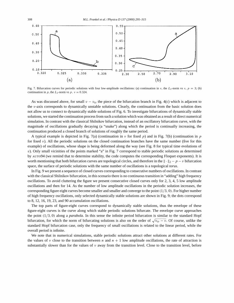
Fig. 7. Bifurcation curves for periodic solutions with four low-amplitude oscillations: (a) continuation inν, theL2-norm vsν, p = 3; (b)continuation inp, theL2-norm vsp, ν = 0.324.

As was discussed above, for smallν − νcr the piece of the bifurcation branch in Fig. 4(c) which is adjacent tothe ν-axis corresponds to dynamically unstable solutions. Clearly, the continuation from the basic solution doesnot allow us to connect to dynamically stable solutions of Fig. 6. To investigate bifurcations of dynamically stablesolutions, we started the continuation process from such a solution which was obtained as a result of direct numericalsimulation. In contrast with the classical Shilnikov bifurcation, instead of an oscillatory bifurcation curve, with themagnitude of oscillations gradually decaying (a “snake”) along which the period is continually increasing, thecontinuation produced a closed branch of solutions of roughly the same period.

A typical example is depicted in Fig. 7(a) (continuation inν for fixed p) and in Fig. 7(b) (continuation inpfor fixed ν). All the periodic solutions on the closed continuation branches have the same number (five for thisexample) of oscillations, whose shape is being deformed along the way (see Fig. 8 for typical time evolutions ofv). Only small vicinities of the points marked “a” in Fig. 7 correspond to stable periodic solutions as determinedby auto94 (we remind that to determine stability, the code computes the corresponding Floquet exponents). It isworth mentioning that both bifurcation curves are topological circles, and therefore in the‖ · ‖2 −p − ν bifurcationspace, the surface of periodic solutions with the same number of oscillations is a topologicaltorus.

In Fig. 9 we present a sequence of closed curves corresponding to consecutive numbers of oscillations. In contrastwith the classical Shilnikov bifurcation, in this scenario there is no continuous transition in “adding” high frequencyoscillations. To avoid cluttering the figure we present consecutive closed curves only for 2, 3, 4, 5 low amplitudeoscillations and then for 14. As the number of low amplitude oscillations in the periodic solution increases, thecorresponding figure eight curves become smaller and smaller and converge to the point(1/3, 0). For higher numberof high frequency oscillations, only selected dynamically stable solutions are shown in Fig. 9; the dots correspondto 8, 12, 16, 19, 23, and 90 accumulation oscillations.

The top parts of figure-eight curves correspond to dynamically stable solutions, thus the envelope of thesefigure-eight curves is the curve along which stable periodic solutions bifurcate. The envelope curve approachesthe point(1/3, 0) along aparabola. In this sense the infinite period bifurcation is similar to the standard Hopfbifurcation, for which the norm of bifurcating solutions is also on the order of

√νcr − ν. Of course, unlike the

standard Hopf bifurcation case, only the frequency of small oscillations is related to the linear period, while theoverall period is infinite.

We note that in numerical simulations, stable periodic solutions attract other solutions at different rates. Forthe values ofν close to the transition betweenn andn + 1 low amplitude oscillations, the rate of attraction issubstantially slower than for the values ofν away from the transition level. Close to the transition level, before


Fig. 8. Typical time historiesv(t) vs t for periodic solutions with four low-amplitude oscillations. The time histories correspond to the pointsmarked “a”, “b”, and “c” in the previous figure.

Fig. 9. A series of bifurcation curves, theL2 norm of periodic solutions for solutions with increasing number of oscillations,p = 3.


Fig. 10. A simple transition from harmonic oscillations to relaxation oscillations, velocity perturbation profiles,v(t) vs t , and projections of theorbits into plane(v, u|x=1), p = 1.5, ν = 0.33, 0.315, and 0.29

settling to a periodic trajectory withn small oscillations, the numerical solution “hesitate” and may pick up, atrandom, different numbers of small oscillations separated by large bursts.

5.3. Supercritical bifurcation (p1 < p < p2)

In the weakly nonlinear regime, the periodic solutions that bifurcate from the trivial solution are harmonicoscillations with the period close to the linear period and the amplitude on the order of

√νcr − ν, as prescribed by

the bifurcation diagram Fig. 4(b). Asν moves into more nonlinear regions however, there is a variety of possibledynamical scenarios, depending on the value of the kinetic parameterp.

For the regimes withp < p3 = 1.92 dynamics are qualitatively similar. They are illustrated by the sequence inFig. 10. Asν decreases, harmonic oscillations gradually become more and more relaxational while their period isgradually increasing.

At p ' 1.92 a new qualitative feature appears which is illustrated in the sequence in Fig. 11. Atν = 0.323 theharmonic periodic solution experiences period doubling. Asν continues to drop, the larger oval of the phase portraitdevelops a characteristic “corner” that corresponds to the burst phase of the infinite period bifurcation sequence.Finally, through the reverse period doubling, a simple periodic solution is created, it contains the periodicallyrepeated burst-like phase alone. Asp increases, this scenario evolves in the following fashion (Fig. 12) : a harmonicoscillation undergoes two period doublings, then the ovals form corners, and through the cascade of two reversedoublings a single burst solution is born. Asp increases further, the scenario of cascade-deformation-reverse cascadewas observed with 3 and 4 period doublings. Apparently, cascades with any 2k number of ovals should exist.

Yet another interesting qualitative feature appears asp increases beyondp = 2.1. First, asν decreases, a periodicsolution undergoes an infinite series of period doubling and becomes chaotic. With the further decrease inν thesolution exits the chaotic regime via an infinite reverse cascade of period doubling that is terminated with a “period3” solution. Asν drops even further, the “period 3” solution undergoes a cascade of period doubling leading to


Fig. 11. A transition from harmonic oscillations to burst like oscillations through direct and reverse period doubling, velocity perturbationprofiles,v(t) vs t and projections of the orbits into the plane(v, u|x=1); p = 2.0, ν = 0.33, 0.324, 0.323, 0.315, 0.3101, and 0.3.

chaos. Asν changes within this chaotic regime, the phase curves deform in such a way that the characteristic “burstcorner” becomes well-pronounced. Again the system leaves the chaotic regime through a reverse period-doublingcascade which is terminated with an accumulation-burst pattern. Depending on the value of parameterp, weobserved patterns with 2, 3, 4, and 5 accumulation oscillations; apparently any number of these oscillations canbe obtained. Finally, asν moves even further into the nonlinear region, the number of accumulation oscillationsis consecutively reduced to two through the mechanism described in Section 5.2. After that the last accumulationoscillation disappears through a reverse period doubling, and a pure burst periodic solution arises. The scenario just


Fig. 12. A transition from harmonic oscillations to burst like oscillations through a cascade of direct and reverse period doubling, velocity pertur-bation profiles,v(t) vst , and projections of the orbits into the plane(v, u|x=1), p = 2.08, ν = 0.326, 0.325, 0.323, 0.3195, 0.3063, and 0.306

described is illustrated in Fig. 13. The second reverse cascade there ends with the burst-accumulation pattern whichcontains three low amplitude oscillations.

6. Conclusion

We have presented a three-dimensional system of ordinary differential equations that reveals very rich dynam-ics and novel mechanisms of exchange of stability. In particular it demonstrates a critical and subcritical Hopfbifurcation, multiple cascades of period doubling, and a novel type of infinite period bifurcation.


Fig. 13. A transition from harmonic oscillations to burst like oscillations through a cascade of direct and reverse period doubling, period3, and another direct-reverse period doubling cascade, velocity perturbation profiles,v(t) vs t , and projections of the orbits into the plane(v, u|x=1), p = 2.3, ν = 0.33, 0.329, 0.3285, 0.3281, 0.32805, 0.328, 0.327, 0.3245, 0.3235, 0.322, 0.315, 0.31, and 0.29.

The system has clear physical origins and approximates dynamics of the underlying infinitely dimensional (pde)problem extremely accurately. This gives a strong indication that the free boundary problem itself possesses afinite-dimensional attractor. We address this issue in a work in progress. We prove that a version of the freeboundary problem on a finite spatial interval does possess a finite-dimensional attractor. Moreover, the dimensiondoes not depend on the length of the interval. These results will appear in the nearest future (see [13]).

We believe the three-dimensional system of ordinary differential equations of the present paper is a very interestingexample of a relatively simple low-dimensional dynamical system that preserves important features of its physically


Fig. 13. (Continued).


motivated and dynamically rich PDE source, even in a variety of strongly nonlinear regimes. It appears that not allthe nonlinearities of the system are of equal importance, and that some of them can be dropped without loosing anydynamical scenarios. It would be very interesting to find a normal form for the system that would allow to clarifythe origin and structure of the unusual dynamics we have discussed in the paper.

Acknowledgements

Michael Frankel would like to acknowledge support in part by NSF through grant DMS-9623006. Gregor Kovacicand Ilya Timofeyev would like to acknowledge support in part from the US Department of Energy through grantDE-FG02-93ER25154, the National Science Foundation through grants DMS-9502142 and DMS-9510728, andthe Alfred P. Sloan Foundation through a Sloan Research Fellowship. Victor Roytburd would like to acknowledgesupport in part by NSF through grant DMS-9704325. The authors are grateful to the referee for several helpfulsuggestions.

References

[1] I. Brailovsky, G. Sivashinsky, Chaotic dynamics in solid fuel combustion, Physica D 65 (1993) 191–198.[2] A. Bayliss, B. Matkowsky, M. Minkoff, Period doubling gained, period doubling lost, SIAM J. Appl. Math. 49 (1989) 1047–1063.[3] M. Bosch, C. Simó, Attractors in a Shilnikov–Hopf scenario and a related one-dimensional map, Physica D 62 (1993) 217–229.[4] E. Doedel, X. Wang, T. Fairgrieve,auto94, Software for continuation and bifurcation problems, Applied Mathematics Report, California

Institute of Technology, 1994.[5] M.L. Frankel, On the nonlinear evolution of a solid–liquid interface, Phys. Lett. A 128 (1988) 57–60.[6] M.L. Frankel, V. Roytburd, Dynamical portrait of a model of thermal instability: cascades, chaos, reversed cascades and infinite period

bifurcations, Int. J. Bifur. Chaos 4 (1994) 579–593.[7] M.L. Frankel, V. Roytburd, G. Sivashinsky, A sequence of period doubling and chaotic pulsations in a free boundary problem modeling

thermal instabilities, SIAM J. Appl. Math. 54 (1994) 1357–1374.[8] M.L. Frankel, V. Roytburd, A free boundary problem modeling thermal instabilities: well-posedness, SIAM J. Math. Anal. 25 (1994)

1357–1374.[9] M.L. Frankel, V. Roytburd, A free boundary problem modeling thermal instabilities: stability and bifurcation, J. Dynamics Differential

Equations 6 (1994) 447–486.[10] M.L. Frankel, V. Roytburd, On a free boundary problem related to solid-state combustion, Comm. Appl. Nonlinear Anal. 2 (1995) 1–22.[11] M.L. Frankel, V. Roytburd, Finite-dimensional model of thermal instability, Appl. Math. Lett. 8 (1995) 39–44.[12] M. Frankel, M. Qu, V. Roytburd, On a free interface problem modeling solid combustion and rapid solidification in infinite medium, in:

Dynamical Systems and Applications, World Scientific series in Applicable Analysis, vol. 4, 1995, pp. 263–278.[13] M.L. Frankel, V. Roytburd, Finite-dimensional attractors for a free boundary model of a thermal instability, in preparation.[14] P. Glendinning, C. Sparrow, Local and global behavior near homoclinic orbits, J. Stat. Phys. 35 (1984) 645–696.[15] S.M. Gol’berg, M.I. Tribelskii, On laser induced evaporation of nonlinear absorbing media, Zh. Tekh. Fiz. (Sov. Phys.-J. Tech. Phys.) 55

(1985) 848-857 (in Russian).[16] D. Gottlieb, S. Orszag, Numerical Analysis of Spectral Methods: Theory and Applications, SIAM, Philadelphia, PA, 1977.[17] P. Hirschberg, E. Knobloch, Shilnikov–Hopf bifurcation, Physica D 62 (1993) 202–216.[18] J.S. Langer, Lectures in the theory of pattern formation, in: J. Souletie, J. Vannimenus, R. Stora (Eds.), Chance and Matter, Elsevier,

Amsterdam, 1987.[19] B.J. Matkowsky, G.I. Sivashinsky, An asymptotic derivation of two models in flame theory associated with the constant density

approximation, SIAM J. Appl. Math 37 (1979) 686–689.[20] A.G. Merzhanov, A.K. Filonenko, I.P. Borovinskaya, New Phenomena in Combustion of Condensed Systems, Dokl. Akad. Nauk USSR,

208 (1973) 892–894 (Soviet Phys. Dokl. 208 (1973) 122–125).[21] A.G. Merzhanov, SHS processes: combustion theory and practice, Arch. Combustionis, 1 (1981) 23-48.[22] K.G. Shkadinsky, B.I. Khaikin, A.G. Merzhanov, Propagation of a Pulsating Exothermic Reaction Front in the Condensed Phase, Combust.

Expl. Shock Waves 7 (1971) 15–22.[23] W. Van Saarloos, J. Weeks, Surface undulations in explosive crystallization: a nonlinear analysis of a thermal instability, Physica D 12

(1984) 279–294.[24] A. Visintin, Stefan problem with a kinetic condition at the free boundary, Annali di Matematica Pura ed Applicata 146 (1987) 97–122.[25] Ia.B. Zeldovich, G.I. Barenblatt, V.B. Librovich, G.M. Makhviladze, The Mathematical Theory of Combustion and Explosions, Consultants

Bureau, Washington, DC, 1985.

Finite-dimensional dynamical system modeling thermal...

Documents

Transcript of Finite-dimensional dynamical system modeling thermal...