
Financial work incentives in Britain
74
FINANCIAL WORK INCENTIVES IN BRITAIN: COMPARISONS OVER TIME AND BETWEEN FAMILY TYPES Stuart Adam Mike Brewer Andrew Shephard THE INSTITUTE FOR FISCAL STUDIES WP06/20
Transcript of Financial work incentives in Britain
FINANCIAL WORK INCENTIVES IN BRITAIN: COMPARISONS OVER TIME AND BETWEEN FAMILY TYPES
Stuart AdamMike Brewe
Andrew Shephard
THE INSTITUTE FOR FISCAL STUDIESWP06/20
r

Financial work incentives in Britain: comparisons over time and between family types
Stuart Adam, Mike Brewer and Andrew Shephard1
Executive Summary
This paper reviews various techniques for quantifying financial incentives to work, shows how financial work incentives have changed across the population since 1979, and estimates how much of these changes are due to changes in the tax and benefit system.
Two aspects of financial work incentives are important: the incentive to be in work at all, and the incentive to progress in work (i.e. increase earnings). We measure the incentive to progress using the effective marginal tax rate (EMTR); we measure the incentive to work at all using the replacement rate (RR) and the participation tax rate (PTR). In all three cases, higher rates correspond to weaker work incentives.
Our measures of incentives incorporate income tax, employee National Insurance contributions, council tax, tax credits and social security benefits; they do not take account of taxes formally incident on companies (such as employer National Insurance contributions) or indirect taxes.
We find that work incentives are generally weaker for people who are not working than for people who are working. However, such analysis requires us to estimate what wages non-workers would command if they did work; concerns about the reliability of these estimates mean that for most of our analysis we restrict attention to people in work.
The weakest work incentives are faced by people on low incomes who face having their means-tested benefits or tax credits withdrawn if they increase their income. Such disincentives are much greater than those imposed on high-income people through higher rates of income tax. Over two million workers in Britain stand to lose more than half of any increase in earnings to taxes and reduced benefits. Some 160,000 would keep less than 10p of each extra £1 they earned.
1 Adam, Brewer and Shephard are all at the Institute for Fiscal Studies. Contact: [email protected]. This paper was produced as part of a project called “Can Governments reduce poverty and improve work incentives?”, supported by the Joseph Rowntree Foundation (JRF) as part of its programme of research and innovative development projects, which it hopes will be of value to policy-makers, practitioners and service users. The facts presented and views expressed in this paper, however, are those of the authors and not necessarily those of the Foundation, nor of the other individuals or institutions mentioned here, including the Institute for Fiscal Studies, which has no corporate view. The authors are very grateful to Chris Goulden, the project manager at JRF, and to the Advisory Group. Howard Reed was originally the manager of the project that led to this report, and the authors are grateful for his contributions. Material from the Family Expenditure Survey (FES) was made available by the Office for National Statistics through the UK Data Archive and has been used by permission of the Controller of HMSO. Material from the Family Resources Survey (FRS) was made available by the Department for Work and Pensions, and is also available at the UK Data Archive.
1

Different groups in society face different work incentives. Lone parents face some of the weakest incentives to work at all, and face weak incentives to earn more, because many will be subject to withdrawal of a tax credit or means-tested benefit as their earnings rise: over two-thirds of working lone parents face an EMTR in excess of 50 per cent. On the other hand, single adults without children face some of the strongest incentives, mostly because they are entitled to relatively little support when they do not work, and because they are not likely to be entitled to tax credits or means-tested benefits when they are in work. People living with a partner and with dependent children tend to have weaker work incentives in general than those without children, partly because they are more likely to be older and earn more, and therefore subject to the higher rate of income tax, but also because they are more likely to be subject to tax credit withdrawal.
Both incentives to work at all and incentives to progress have strengthened, on average, since 1979, but have weakened on average since 2000. Only part of these changes in work incentives are the direct result of tax and benefit reforms: changes in average wages, wage inequality, rent levels and working patterns within two-adult families are also important explanatory factors.
Separating out these various factors shows that tax and benefit reforms since 1979 have strengthened work incentives on average, although the precise trends vary by family type. Across the whole population, reforms under the Conservatives acted to strengthen average work incentives whereas Labour’s reforms to date have acted to weaken average work incentives. On average, tax and benefit changes since 1997 mean that someone choosing to work harder gets to keep 2½p less of each extra £1 they earn. However, these trends have not been uniform: the Conservatives’ reforms weakened work incentives for a period in the early 1980s, and Labour’s reforms have strengthened incentives for lone parents to work at all, and have strengthened incentives to earn more for some groups previously facing the weakest incentives.
Growth in real wages over the period has tended to strengthen average incentives to work at all (as measured by replacement rates), but has had little effect on average incentives to progress, weakening them very slightly overall. Other changes in the economy, such as the growth in real rents acting through housing benefit, have tended to weaken both the incentive to work at all and the incentive to progress.
2

Contents
1. Introduction...........................................................................................................................4
2. Measuring financial work incentives ..................................................................................6
2.1. Defining our main measures of financial work incentives.....................................6
2.1.1 The incentive to work at all ...................................................................................6
2.1.2 The incentive to progress in the labour market ..................................................8
2.2. Relating work incentive measures to the budget constraint ..................................9
2.3. Financial work incentives in Britain in 2005: an overview...................................12
2.3.1 Work incentives for all working adults...............................................................12
2.3.2 How do work incentives vary by family circumstances? .................................14
2.4 Detailed issues around measuring financial work incentives...............................19
2.4.1 How do we define “net income”?.......................................................................19
2.4.2 What “margin” should be used when calculating effective marginal tax rates?......................................................................................................................................23
2.4.3 What time period should be considered when measuring incomes? .............24
2.4.4 How should we estimate work incentives for those not working? ................26
3. Work incentives over time.................................................................................................29
3.1 What has happened to financial work incentives on average? ............................29
The incentive to work at all ...............................................................................................30
The incentive to progress...................................................................................................36
3.2 How have financial work incentives changed for different groups in the population? ...............................................................................................................................39
Lone parents: incentive to work at all ..............................................................................39
Lone parents: incentive to progress .................................................................................43
Couples with children: incentive to work at all...............................................................46
Couples with children: incentive to progress ..................................................................51
Single people without children: incentive to work at all................................................55
Single people without children: incentive to progress ...................................................58
Couples without children: incentive to work at all.........................................................60
Couples without children: incentive to progress ............................................................66
3.3 Bringing it all together...............................................................................................70
References .....................................................................................................................................72
3
1. Introduction Since 1997, the UK Government has made a series of changes to taxes and benefits with the twin aims of reducing child and pensioner poverty and ‘making work pay’. Much is known about how recent tax and benefit changes in the UK have contributed to changes in poverty and inequality. 2 Less is known about how those same reforms have affected financial incentives to work. 3 This paper reviews various techniques for quantifying financial incentives to work, shows how financial work incentives have changed across the population since 1979, and estimates how much of these changes are due to changes in the tax and benefit system. The material in this paper is summarised and built upon in Adam et al (2006), which also explores the trade-off between strengthening work incentives and redistributing income.
Economists usually think of tax and benefit programmes as affecting work incentives in two ways: through an income effect and a substitution effect. The income effect refers to the idea that higher taxes or lower benefits make people worse off and so more inclined to seek to increase their earnings to make up for this lost income. The substitution effect refers to the idea that income taxes or means testing discourage work by reducing the reward for additional work: higher incomes can only be obtained with a greater increase in hours worked or work effort because recipients see some of the gain from increasing their private income taken in tax or offset by reductions in tax credit and benefit entitlement. Some models attempt to make inferences about the size of income and substitution effects based on individuals’ responses to past tax and benefit changes (see Brewer et al (2005a) for an example, and Blundell and MaCurdy (1999) for a wider review), and it is these sorts of models that tell us that financial incentives do matter to individuals’ – and especially mothers’ – decisions of whether and how much to work. But all such estimates remain controversial and laden with assumptions, and we do not espouse any here. In this paper, therefore, we estimate only the direct effects of policies on work incentives: we do not estimate how far people respond to these incentives and therefore the ultimate effect of policies on employment and earnings.
The rest of the report is structured as follows: Chapter 2 reviews various techniques of quantifying the financial incentives to work, and shows how financial work incentives vary across the population in 2005–06. Chapter 3 shows the key trends since 1979, and estimates how much of the changes are due to changes in the tax and benefit system.
Much of our analysis is based on measures of work incentives produced by the IFS’s tax and benefit micro-simulation model, TAXBEN. TAXBEN is able to use data from Family Resources Survey and the Family Expenditure Survey. The Family Resources Survey an annual cross-section survey of 27,000 households in Great Britain, and began in 1994. The Family Expenditure Survey is an annual cross-section survey of around 2 See Brewer, Goodman, Shaw and Sibieta (2006) on the income distribution and relative poverty now, Sutherland et al (2004) or Brewer, Clark and Goodman (2002) on how tax and benefit changes have affected child poverty, and Clark and Leicester (2004) on how tax and benefit changes have affected inequality.
3 The impact of the working families’ tax credit and related reforms on lone parents has been thoroughly investigated by a number of studies, and recent work by some of the authors of this report has examined how tax and benefit changes since 1997 have affected work incentives across the population. See Brewer and Browne (2006) for a review of the former, and Brewer and Shephard (2004, 2005) for the latter.
4

7,000 households in the UK, available from the 1960s through to 2000–01. The analysis uses the Family Expenditure Survey until 1993, and the Family Resources Survey between 1994–95 and 2002–03. Years refer to calendar years until 1993, and then financial years. Synthetic data for 2003–04 – 2005–06 was created by uprating data from 2002–03, as described in Brewer, Browne and Sutherland (2006). The analysis of work incentives in this report is restricted to working individuals in families in which no-one is self-employed, aged over 55 or receiving a disability benefit. Individuals with particularly complicated budget constraints, who did not have an hourly wage or who had extreme values of measures of work incentives were also omitted from the analysis. Details of the final samples used are available from the authors.
5

2. Measuring financial work incentives This chapter defines some important measures of financial work incentives (2.1-2.2), and presents an overview of financial work incentives in Britain in 2005 (2.3), showing what types of people tend to face strong or weak financial work incentives. It also discusses a number of detailed issues involved when measuring financial work incentives using a micro-simulation model (2.4).
2.1. Defining our main measures of financial work incentives
An individual’s financial incentive to work will depend on the shape of the relationship between hours of paid work and net income, taking account of the financial costs of working and not working.4 This relationship is known as a “budget constraint”: see Figure 2.1a for an example. Budget constraints tell us all we might want to know about the financial incentives to work for an individual, but it is often preferable to summarise this information in some convenient measure. When doing so, there are two important dimensions of the budget constraint that we attempt to quantify:
• the financial reward for working compared to not working, measured by some function of incomes in and out of work, which we call the incentive to work at all.
• The incentive to for those in work to work harder or earn more, which we call the incentive to progress in the labour market.
2.1.1 The incentive to work at all
Two common measures of the incentive to work at all are the replacement rate, and the participation tax rate: 5
i. The replacement rate (RR) is measured by (net income out of work) / (net income in work). For example, if someone would receive £50 in benefits if they did not work, and would have a net income of £200 if they worked, then the replacement rate is 50/200 or 0.25.
ii. The participation tax rate (PTR) is measured by 1 – {(net income in work – net income out of work) / gross earnings}, or one minus the financial gain to working as a proportion of gross earnings. It measures the proportion of gross earnings taken in tax or reduced benefits. To continue the previous example, if that person had gross earnings of £250, then the participation tax rate would be 1 – (200-50)/250, or 0.4.
A number of points apply to both of these measures:
4 “Net income” means income after benefits and tax credits have been added and after direct taxes have been deducted.
5 Gregg et al (1999) call the latter concept the average tax rate, although the average tax rate is usually defined to mean total tax paid divided by total gross income, with no reference to out-of-work benefits or tax credits forgone.
6
• “net income” means income after benefits and tax credits have been added and after direct taxes have been deducted.
• Low numbers of both mean stronger financial incentives to work: a participation tax rate of zero would mean that an individual got to keep all of their gross earnings, and lost no benefits or tax credits, when they worked; a replacement rate of zero occurs where someone has no income if they do not work. At the other extreme, a PTR or an RR of one would mean that there is no financial reward to working. High PTRs or RRs are often referred to as the unemployment trap.
• Interpreting differences in these measures between individuals who are working different numbers of hours can be problematic, and this is why, in the later empirical analysis, we hold hours of work constant when comparing these measures between individuals and over time.
• Calculating either measure for non-workers requires assumptions about what they would earn if they did work.
• For individuals in couples, we can calculate the replacement rate and participation tax rate using individual or family income, and this choice will affect our impression of the strength of the financial reward to work. For example, a low-earning person living with a high-earning partner may have no independent income if he or she does not work, and therefore would have a very low replacement rate – or a strong financial incentive to work – when calculated using individual income. However, the same individual would have a very high replacement rate when calculated using family income, because whether he or she works makes little difference proportionally to the family’s income. By contrast, the participation tax rate for this individual is likely to be very low (if the individual is only paying income tax and employee national insurance contributions on a small portion of their earnings, and is in a family too rich to be entitled to tax credits) regardless of whether individual or family income is used for the calculation.
Both these measures attempt to capture the incentive to work at all, but they are different, and as a result of this, these measures behave differently following different sorts of changes in income. In particular:
• A constant increase in income at all hours (in other words, an equal cash gain in in-work and out-of-work incomes, or a vertical shift in the budget constraint) does not change the participation tax rate, but increases the replacement rate. This means that the PTR would suggest no change in incentives, but the RR that they have got weaker.
• At a given level of hours of work, an increase in the gross hourly wage will strengthen incentives according to the RR, but will have ambiguous effects according to the PTR.
7
According to economic theory, the impact of an equal cash gain in in-work and out-of-work incomes should be to reduce the attractiveness of working compared to not working, and the impact of an increase in the hourly wage should be the reverse. This means, then, that for these two very simple thought experiments, the replacement rate accords with the intuition from simple economic theory. However, the participation tax rate better captures how the tax and benefit system affects the incentive to work: it distinguishes between whether a reduced reward to work is caused by higher taxes or lower wages, for example, which the replacement rate does not. And, as discussed above, the two measures can give very different impressions of the incentive to work faced by adults in a couple. Therefore, much of the empirical analysis that follows will use both measures.
Other ways of measuring the incentive to work at all There are other ways of measuring the financial incentive to work at all, such as the financial gain to work (the difference between income in work and income out of work) and the average tax rate (total taxes paid (less in-work benefits received) divided by gross earnings). Like the RR and PTR, these are convenient ways of summarising the shape of the budget constraint. In addition, in a rather specialised study, Giles et al (1996) analysed the work incentives facing adults in rented accommodation by estimating the number of weekly hours of work needed to exhaust entitlement to housing benefit. Housing benefit is important when considering work incentives because recipients of housing benefit face a high EMTR until their incomes have risen to the point where they are no longer entitled. The measure used in Giles et al (1996) attempts to capture how far these high EMTRs affect an individual. Clearly, the more hours that must be worked until entitlement is exhausted, the weaker is the incentive to work. Individuals with high wages and low rents will need to work fewer hours before entitlement is exhausted. The drawbacks of this measure are, though, that it’s rather arbitrary, and very specific to a particular set of individuals, and a specific tax and benefit system: not all individuals are entitled to housing benefit, even when they have a low income.
2.1.2 The incentive to progress in the labour market
The incentive for those in work to progress in the labour market can be measured by the effective marginal tax rate (EMTR), the slope of the budget constraint. The EMTR measures how much of a small change in earnings is lost to direct tax payments and foregone state benefit and tax credit entitlements, and it tells us about the strength of the incentive for individuals to increase their earnings slightly, whether through working more hours, or through promotion, qualifying for bonus payments or getting a better-paid job. In this paper, we use the term “incentives to progress” for all these possibilities.
As with the incentive to work at all, low numbers mean stronger financial incentives. An EMTR of zero means that the individual keeps all of any small change in earnings, and a rate of 1 (or 100%) means that the individual keeps none. High EMTRs amongst workers in low-income families are often referred to as the poverty trap.
Another measure of the incentive to progress would be the net hourly wage: the amount (in £) by which an individual’s net income would rise were she to work an extra hour.
8

Like the RR relative to the PTR, this can sometimes accord better with economic theory than the EMTR: for example, a rise in the gross hourly wage will affect the net wage in the same way as a fall in the tax rate (unlike with the EMTR), reflecting the prediction from economic theory that people will respond in the same way to both changes. We do not use this measure because of the difficulty in understanding changes in the net wage over a period when gross wages have changed markedly: it is more useful when comparing incentives to progress at a point in time. 6
2.2. Relating work incentive measures to the budget constraint
All the standard work-incentives measures can be related to – and derived from – a standard budget constraint diagram. The four diagrams below show the relationship between the budget constraint (the relationship between gross earning and net income after taxes and benefits) and the three main measures of work incentives discussed here. Figure 2.1a shows a hypothetical budget constraint (for a lone parent with 1 child aged 3 earning £6 an hour with no housing benefit entitlement, no formal childcare costs, but liable to average (England and Wales)Band D council tax, all under the April 2005 tax and benefit system).
The EMTR – our measure of incentives to progress in the labour market – is reflected in the slope of this line, and is shown in Figure 2.1b. EMTRs of 100% occur when an individual is entitled to income support and every pound of private earnings above the disregard reduces the income support payment by a pound.
Figure 2.1a. A budget constraint for a lone parent with 1 child, April 2005 tax and benefit system
£0
£75
£150
£225
£300
£375
0 10 20 30 40 5Hours worked
Net
wee
kly
inco
me
a
0
b
c
Notes and sources: a and c are the levels of gross earnings and net income respectively for this person if they work 16 hours, and b is their net income (from benefits) if they do not work. Authors’ calculations
6 A measure that reflects the changing slope of the budget constraint is its convexity. Budget constraints are convex when EMTRs rise with incomes, so a measure of convexity tells us how quickly EMTRs rise or fall with income: studies including Zarutskie (2003) and Hubbard and Gentry (2004) have used it as a measure of how well the tax and benefit systems provides insurance against income risk.
9
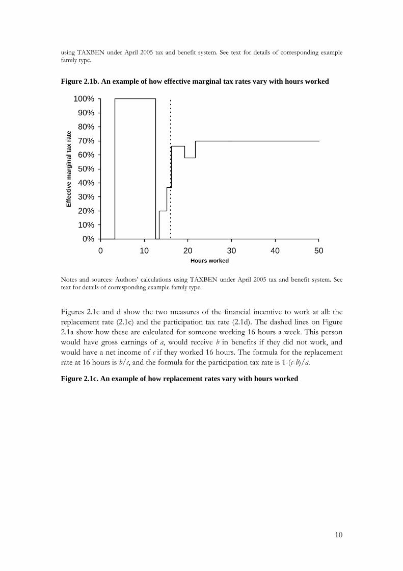
using TAXBEN under April 2005 tax and benefit system. See text for details of corresponding example family type.
Figure 2.1b. An example of how effective marginal tax rates vary with hours worked
0%
10%
20%
30%
40%
50%
60%
70%
80%
90%
100%
0 10 20 30 40 5Hours worked
Effe
ctiv
e m
argi
nal t
ax ra
te
0
Notes and sources: Authors’ calculations using TAXBEN under April 2005 tax and benefit system. See text for details of corresponding example family type.
Figures 2.1c and d show the two measures of the financial incentive to work at all: the replacement rate (2.1c) and the participation tax rate (2.1d). The dashed lines on Figure 2.1a show how these are calculated for someone working 16 hours a week. This person would have gross earnings of a, would receive b in benefits if they did not work, and would have a net income of c if they worked 16 hours. The formula for the replacement rate at 16 hours is b/c, and the formula for the participation tax rate is 1-(c-b)/a.
Figure 2.1c. An example of how replacement rates vary with hours worked
10

40%
50%
60%
70%
80%
90%
100%
0 10 20 30 40 5Hours worked
Rep
lace
men
t rat
e
0
Notes and sources: Authors’ calculations using TAXBEN under April 2004 tax and benefit system. See text for details of corresponding example family type.
Figure 2.1d. An example of how the participation tax rate varies with hours worked
-10%
0%
10%
20%
30%
40%
50%
60%
70%
80%
0 10 20 30 40 5Hours worked
Part
icip
atio
n ta
x ra
te
0
Notes and sources: Authors’ calculations using TAXBEN under April 2004 tax and benefit system. See text for details of corresponding example family type.
11

2.3. Financial work incentives in Britain in 2005: an overview
This section presents an overview of financial work incentives for people working in Britain in 2005, showing what types of people tend to face strong or weak financial work incentives. We begin by showing the distribution of replacement rates, participation tax rates and effective marginal tax rates amongst working age adults under the April 2005 tax and benefit system. We then show how the distribution of work incentives varies between different family types. Full details of the way we construct these measures is given in section 2.4, which also shows how different ways of estimating work incentives in a micro-simulation model affect our impression of the distribution of work incentives in Britain.
2.3.1 Work incentives for all working adults
The distribution of replacement rates is shown in Table 2.1. The most common range of replacement rates faced by working-age working adults in 2005 is between 50% and 60%, where around 2.75 million adults are located (this means that these adults’ families would receive 50-60% of their current income if the individual stopped work). Almost 70% of individuals face replacement rates between 20% and 70%, and the distribution of replacement rates is roughly symmetric: there is a similar number of people with very high replacement rates (weak work incentives) as with very low replacement rates (strong work incentives).
Amongst the population as a whole, there are several factors that lead to this variation in replacement rates: individuals could be facing high replacement rates if they have a low wage, only work a few hours every week, or if the tax and benefit systems means that they face high levels of out-of-work income. Understanding the variation in replacements rates is much more straightforward when examining the incentives within different family groups, because most of the variation in replacement rates within family groups is derived from variation in wages.
Table 2.1. Replacement rates amongst working adults Number of working adults with rate in
this band Number who face rate in or higher than this band
0% 50,000 17,800,000 0.1% - 10% 470,000 17,740,000 10.1% - 20% 1,640,000 17,270,000 20.1%–30% 2,400,000 15,630,000 30.1%–40% 2,180,000 13,230,000 40.1%–50% 2,640,000 11,050,000 50.1%–60% 2,750,000 8,410,000 60.1%–70% 2,100,000 5,660,000 70.1%–80% 1,690,000 3,560,000 80.1%–90% 1,270,000 1,870,000 90.1%–100% 560,000 600,000 Over 100% 40,000 40,000 All 17,800,000
Notes and sources: Authors’ calculations using FRS 2002–03 and TAXBEN under April 2005 tax and benefit system. Excludes adults aged over 55, the self-employed, adults receiving a disability benefit, and other adults living in these families. Figures grossed up using FRS weights and rounded to nearest 10,000. Numbers may not add because of rounding. See section 2.4 for details.
12

Table 2.2 shows that the most common participation tax rate band is between 30% and 40%, with 5.1 million individuals facing rates in this range. Unlike the distribution of replacement rates, the distribution of participation tax rates is skewed to the lower end.
Table 2.2. Participation tax rates amongst working adults Number of working adults with rate in
this band Number who face rate in or higher than this band
0% 500,000 17,800,000 0.1% - 10% 570,000 17,320,000 10.1% - 20% 1,450,000 16,750,000 20.1%–30% 4,490,000 15,300,000 30.1%–40% 4,610,000 10,810,000 40.1%–50% 2,870,000 6,200,000 50.1%–60% 1,610,000 3,330,000 60.1%–70% 850,000 1,720,000 70.1%–80% 520,000 870,000 80.1%–90% 260,000 350,000 90.1%–100% 50,000 90,000 Over 100% 40,000 40,000 All 17,800,000
Notes and sources: Authors’ calculations using FRS 2002–03 and TAXBEN under April 2005 tax and benefit system. Excludes adults aged over 55, the self-employed, adults receiving a disability benefit, and other adults living in these families. Figures grossed up using FRS weights and rounded to nearest 10,000. Numbers may not add because of rounding. See section 2.4 for details. Table 2.3 shows the distribution of EMTRs.7 This distribution has a large spike at tax rates of between 30% and 40%: nearly two thirds of working adults have EMTRs in this range. This can be easily understood in terms of the parameters of the tax and benefit system: the single most common EMTR faced by workers under the April 2005 tax and benefit system is 33 per cent, the rate that applies to adults whose own earnings are high enough to pay basic-rate income tax, but lower than the upper earnings limit in national insurance, and with a family income sufficiently high that they have no entitlements to means-tested benefits or tax credits (beyond the family element of the child tax credit). This band also includes people who pay the higher-rate of income tax and are contracted out of the state second pension.
7 Table 4.2 of HMT (2006) shows similar estimates. The key differences between the two tables are that:: a) the Treasury’s estimates only apply to people working at least 16 hours a week; ours apply to anyone working any hours; b) the Treasury’s estimates count the number of families, ours count the number of workers; c) the Treasury’s estimates incorporate some non-take-up of tax credits and means-tested benefits, ours assume full-take-up.
13

Table 2.3. Effective marginal tax rates (EMTRs) amongst working adults Number of working adults with rate in
this band Number who face rate in or higher than this band
0% 560,000 17,800,000 0.1% - 10% 110,000 17,240,000
10.1% - 20% 250,000 17,130,000 20.1%–30% 1,640,000 16,880,000 30.1%–40% 10,900,000 15,240,000 40.1%–50% 2,130,000 4,340,000 50.1%–60% 240,000 2,210,000 60.1%–70% 1,390,000 1,970,000 70.1%–80% 180,000 580,000 80.1%–90% 240,000 400,000
90.1%–100% 120,000 160,000 Over 100% 40,000 40,000
All 17,800,000 Notes and sources: Authors’ calculations using FRS 2002–03 and TAXBEN under April 2005 tax and benefit system. Excludes adults aged over 55, the self-employed, adults receiving a disability benefit, and other adults living in these families. Figures grossed up using FRS weights and rounded to nearest 10,000. Numbers may not add because of rounding. Marginal effective tax rates calculated by increasing hours of work by 5%. See section 2.4 for details. EMTRs of 20% or below – which apply to just under 5% of working adults – are faced by low-earning adults who earn too little to pay basic-rate income tax, and who live either in families who are too rich to be subject to withdrawal of in-work support (because they live with a high-earning partner) or on families whose joint income is sufficiently low so that the adults are not subject to a withdrawal or means-tested benefits or tax credits (in other words, these are low-earning individuals in either very low-income or relative high-income families).
EMTRs between 40% and 50% - which is the second most numerous range of marginal tax rates - tend to apply to adults who earn enough to pay the higher rate of income tax. EMTRs beyond this – and there are around 2.2m workers who face EMTRs in excess of 50 per cent – almost always arise when adults live in a family whose income means that they face a withdrawal of a means-tested benefit or a tax credit. Indeed, the highest EMTRs arise when adults are eligible for more than one means-tested benefit or tax credit, usually housing benefit or council tax benefit in conjunction with tax credits: in April 2005, an individual facing simultaneous withdrawal of tax credits and housing benefit as well as basic rate income tax and standard rate NICs would face an effective marginal tax rate of 89.5% – or 95.5% if they also faced withdrawal of council tax benefit. Most working adults in receipt of income support are subject to a 100% marginal tax rate, as every pound of private earnings above the small disregard is wholly offset by a one pound reduction in their income support entitlement.
2.3.2 How do work incentives vary by family circumstances?
Section 2.3.1 examined the distribution of work incentives across the working population; this section shows how incentives vary by family type.
14

Table 2.4 shows the mean, median and quartile points of replacement rates, participation tax rates and effective marginal tax rates for people in six different family types:8
• single adults without children9
• men and women (separately) in couples without children
• lone parents
• men and women (separately) in couples with children.10
We use these same groups in the next chapter, when we show how work incentives have changed over time.
The financial work incentives of these groups are very different. Lone parents face some of the weakest incentives to work at all, and face weak incentives to progress in the labour market. They face weak incentives to progress because many working lone parents will be subject to withdrawal of a tax credit or means-tested benefit as their earnings rise. For the same reason, and because of the low average wage that they receive and high levels of out-of-work income, they face weak incentives to work at all.
Meanwhile, single adults without children face some of the strongest incentives. The relatively low level of state support that is provided to this group when that they are not working means that their replacement rates are generally low. The incentive to progress is relatively strong for this group, with most individuals being subject just to the basic rate of income tax and National Insurance contributions. The incentive to progress is weaker for high wage individuals who pay the higher rate of income tax, and also for very low-earning individuals who may be receiving a means-tested benefit or working tax credit.
The table gives a mixed impression about the incentive to progress for people in couples. Looking at men in couples first, it can be seen that those who live in families with children have a weaker incentive to progress than those who do not. This is partly because men who live in couples with dependent children tend to be older, and so more likely to be subject to the higher-rate of income tax and therefore face a higher EMTR. Furthermore, men who live in couples with dependent children are much more likely to be subject to tax credit withdrawal. Men in couples with dependent children also face a weaker incentive to work at all (measured by both the replacement rate and the participation tax rate) than those without, because those with children would usually be entitled to tax credits even if no one in the family is working.
8 The median (50th centile) is the middle number, such that half of individuals have higher replacement rates (say) than this and half have lower. Similarly the first quartile (25th percentile) is the number that 25% of replacement rates are below, and the third quartile (75th centile) is the number that 75% of replacement rates are below
9 “Children” means “dependent children”.
10 For brevity, se sometimes refer to these as “fathers in couples” and “mothers in couples” respectively.
15

Table 2.4. Financial work incentives of working adults in different family types, April 2005
RR PTR EMTR Single adults without children
Mean 33.9 46.8 35.1 Median 25.9 39.6 33.0
25th centile 18.7 35.8 31.4 75th centile 37.6 50.0 33.0
Men in couples without children Mean 43.0 29.0 33.8
Median 43.2 26.8 33.0 25th centile 33.8 23.9 31.4 75th centile 51.7 31.8 33.0
Women in couples without children
Mean 59.6 22.3 31.1 Median 58.5 22.1 31.4
25th centile 50.0 17.0 31.4 75th centile 68.8 25.40 33.0
Lone parents Mean 64.2 33.8 56.7
Median 64.3 45.1 68.4 25th centile 50.2 21.8 33.0 75th centile 79.7 56.0 70.0
Fathers in couples Mean 52.4 45.2 42.0
Median 52.1 42.7 33.7 25th centile 41.2 34.4 31.4 75th centile 63.9 54.3 47.0
Mothers in couples Mean 72.6 23.4 33.0
Median 73.9 23.2 33.0 25th centile 62.9 13.0 31.4 75th centile 82.9 33.5 37.0
All Mean 49.4 36.6 36.4
Median 48.5 35.4 33.0 25th centile 29.5 25.5 31.4 75th centile 65.4 45.5 39.1
Notes and sources: Authors’ calculations using FRS 2002–03 and TAXBEN under April 2005 tax and benefit system. Excludes families containing any adults aged over 55, the self-employed, or adults receiving a disability benefit. Marginal effective tax rates calculated by increasing hours of work by 5%. RR = replacement rate. See section 2.4 for details. PTR = participation tax rate. EMTR = effective marginal tax rate.
A similar pattern exists for women in couples: those in families with dependent children tend to face higher EMTRs and higher RRs than those in families with no dependent children. However, an important feature of the work incentives faced by women in couples is the different impressions given by the RR and the PTR: incentives to work at
16

all appear quite weak when considering the replacement rate, but seem relatively strong when considering the participation tax rate. This is because women in couples are much more likely than men to have working (and high-earning) partners, and so the decision to work of a woman in a couple – especially if part-time or for a relatively low wage – may make little difference to family income, while these small additional earnings may be subject to little income tax or National Insurance contributions, and may make no difference to the family’s tax credit entitlement.
Figures 2.2 to 2.4 provide a convenient way of summarising the distribution of work incentives. Figure 2.1 shows the distribution of replacement rates within family types under the April 2005 tax and benefit system. The lines shown are the fraction of individuals (of that family type) with RRs equal to or lower than a given amount. Lines towards the top left of the picture correspond to groups with low RRs (strong incentives).
Figure 2.2. Cumulative distribution of replacement rates within family types, April 2005
0%10%20%30%40%50%60%70%80%90%
100%
0 10 20 30 40 50 60 70 80 90 100
Replacement Rate (%)
% o
f wor
kers
Single adult Lone parentMan, couple no kids Woman, couple no kidsMan, couple with kids Woman, couple with kids
Notes and sources: Authors’ calculations using FRS 2002–03 and TAXBEN under April 2005 tax and benefit system. Excludes families containing any adults aged over 55, self-employed, or receiving a disability benefit. See section 2.4 for details.
Similarly, Figure 2.3 shows the distribution of participation tax rates. Some key findings are:
• Women in couples have some of the lowest participation tax rates. Almost 80% of women in couples without dependent children, and over 60% of those in couples with dependent children, have participation tax rates of 30% or below. In contrast, single adults and men in couples are especially unlikely to face very low participation tax rates.
17

• Across all groups, very few individuals face participation tax rates of 80% or above. The group most likely to have such rates however, is single adults, where they affect almost 4% of these individuals.
• The most common participation tax rate faced by lone parents is 50% to 60%. For other groups it is lower: for women in couples (both with and without children) and men in couples without children, the most common rate band is 20% to 30%, for single adults it is 30% to 40%, and for men in couples with dependent children, it is 40% to 50%.
Figure 2.3. Cumulative distribution of participation tax rates within family types, April 2005
0%10%20%30%40%50%60%70%80%90%
100%
0 10 20 30 40 50 60 70 80 90 100
Participation Tax Rate (%)
% o
f wor
kers
Single adult Lone parentMan, couple no kids Woman, couple no kidsMan, couple with kids Woman, couple with kids
Notes and sources: Authors’ calculations using FRS 2002–03 and TAXBEN under April 2005 tax and benefit system. Excludes families containing any adults aged over 55, self-employed, or receiving a disability benefit. See section 2.4 for details.
Finally, we present the distribution of effective marginal tax rates within different family types in Figure 2.4. Some key findings are:
• The vast majority of mothers in couples, men and women in couples without children, and single adults without children face an EMTR between 30% and 40%. A rate in this band is less common amongst men in couples with children, and relatively few lone parents face such rates.
• Almost 30% of men in couples with children and around 20% of men in couples without children face an EMTR between 40% and 50% (individuals in this range are mostly higher-rate income tax payers). For all other groups, the relevant proportion is under 10%, and is lowest for lone parents.
18

• The proportion of individuals facing low EMTRs (below 30%) is highest amongst women in couples.
• The proportion of individuals facing high EMTRs (above 50%) is highest amongst lone parents: over 60% of such individual are affected.
Figure 2.4. Cumulative distribution of effective marginal tax rates within family types, April 2005
0%10%20%30%40%50%60%70%80%90%
100%
0 10 20 30 40 50 60 70 80 90 100
Effective Marginal Tax Rate (%)
% o
f wor
kers
Single adult Lone parentMan, couple no kids Woman, couple no kidsMan, couple with kids Woman, couple with kids
Notes and sources: Authors’ calculations using FRS 2002–03 and TAXBEN under April 2005 tax and benefit system. Excludes families containing any adults aged over 55, self-employed, or receiving a disability benefit. Marginal effective tax rates calculated by increasing hours of work by 5%. See section 2.4 for details.
2.4 Detailed issues around measuring financial work incentives
The following section discusses a number of detailed issues that need to be confronted when measuring financial work incentives using micro-simulation models.
2.4.1 How do we define “net income”?
All the measures discussed in this chapter relate to an individual’s income at various hour points. This prompts the obvious question of how one should actually measure income. For our analysis we consider all private sources of income in our definition, treating a pound of income the same regardless of whether it was obtained from earnings, investments, or any other source. To derive net income we then deduct income tax, employee National Insurance contributions (NICs) and council tax, and add income from state benefits and tax credits. We do not take account of indirect taxes. Nor do our measures of work incentives take account of taxes formally incident on employers, such as employer NICs; this could be done by adding employer NICs back into gross income.
19

Non-take-up of benefits The example budget constraint shown in Figure 2.1a and the analysis in Section 2.4 were constructed assuming complete take-up of benefits and tax credits. However, welfare programmes do exist where take-up is far from complete. Clearly, our assumption about take-up will have implications for our analysis, as it will determine the shape of the budget constraint and the derived work incentive measures: if we are incorrectly assuming that individuals are claiming and receiving benefits for which they are entitled, then we may be making incorrect inferences about the work incentives that they face. 11 Despite this concern, we assume that there is full take-up of benefits and tax credits. While this assumption clearly is not ideal, given that we do not have complete data on benefit take-up over the past 25 years, it is perhaps the least arbitrary assumption that one can make.
Childcare costs and the costs of working Our main analysis in section 2.4 ignored the fact that there are financial costs of working. Most individuals bear unavoidable various work-related costs, such as transportation costs and work clothing. Any measure of work incentives should ideally take these costs into consideration, and any analysis of the change in work incentives over time needs to factor in trends in these work-related costs: if income in work has been increasing over time, but the costs of working have been increasing more quickly, then it would be difficult to argue that work incentives have actually strengthened. However, most work costs are not recorded in household surveys, making it difficult to incorporate these work-related costs into our micro-simulation analysis. Also, even if we were to observe all work costs faced by those adults in work, the costs of working for someone who is not working (if they did work) may be different from the costs faced by someone who is actually working: this would have to be addressed using a technique similar to that used to solve the problem of the unknown wages for those not currently working (see later this section).
An important work-related cost for parents is the need to arrange and possibly pay for someone else to look after their children while the parents work. Unlike other work-related costs, recent household surveys do record what parents spend on childcare. But there are still difficulties in using this data when calculating work incentives, beyond those already mentioned:
• Parents observed using childcare may be doing so for non-work-related reasons. If so, then it would be wrong to attribute the cost of childcare as a work-related cost. However, household survey data is rarely rich enough to discriminate between these different uses.
• The survey that we use for our comparisons of work incentives over three decades (the FES) does not have such rich data on childcare costs as other surveys that now exist.
11 It is not possible to say which way our results will be biased by assuming full take-up of means-tested benefits and tax credits: the direction of the bias depends on the detail of the particular means-tested benefit/tax credit.
20

However, we show below what impact childcare costs can have upon work incentives estimated by a micro-simulation model. We predict childcare costs for those not working by estimating a relationship between spending on childcare and hours of work (using an Ordinary Least Squares regression, with no correction for “selection effects”), and we assume that all childcare costs recorded in the Family Resources Survey are work-related, so they would not be incurred were the adults not to work.
Figure 2.5 shows the impact on the distribution of replacement rates for lone parents: deducting childcare costs from net incomes when women with dependent children work induces a rightward shift of the distribution, increasing the replacement rate (weakening work incentives) at the median by around 5 percentage points. A similar pattern is observed for adults in couples with dependent children: median replacement rates increase by 6 and 9 percentage points respectively. The percentage point impact is greater when we examine the participation tax rate: for lone parents, women and men in couples with dependent children it increases at the median by 11, 18 and 18 percentage points respectively (full tables are available on request).
Figure 2.5. The replacement rate distribution for working lone parents before and after deducting childcare costs
0%
1%
2%
3%
0.0 0.5 1.0Replacement rate
Perc
enta
ge o
f wor
king
lone
par
ents
Childcare Expenditure No Childcare Expenditure
Notes and sources: Authors’ calculations using FRS 2002–03 and TAXBEN under April 2002 tax and transfer system. Excludes families containing any adults aged over 55, self-employed, or receiving a disability benefit. Figure has been smoothed using kernel density techniques, so it shows the fraction of lone parents with RRs of a given value.
Childcare costs (and other costs of work) clearly have a negative and important impact on work incentives. But while they appear important, our main analysis in chapter 3 will not take them into consideration when calculating work incentives, both for the reasons given above and also because we lack suitable data that covers our 25 year span.
21

Housing costs In the Government’s Households Below Average Income (HBAI) publication, disposable income measures are presented on both a Before Housing Costs (BHC) and an After Housing Costs (AHC) basis. These two different income measures are generally seen as being complementary indicators of changes and differences in living standards over time: the reason for using these different income measures is discussed in Brewer et al (2005b).
The housing services that individuals consume will (in the short run) not be affected by the choice of their hours of work. This means that reflecting housing costs in a budget constraint leads to a uniform downward shift in the budget constraint, with predictable effects on the work inventive measures: the participation tax rate and EMTR will remain unchanged, but replacement rates will fall. We do not deduct housing costs from our measure of net incomes in the main analysis in this paper, but Figure 2.6 shows this predictable shift in the distribution of replacement rates amongst all workers.
Figure 2.6. Replacement Rate Distribution: All Workers (with and without Housing Costs)
0%
1%
2%
3%
0.0 0.5 1.0Replacement rate
Per
cent
age
of w
orke
rs
Housing Costs No Housing Costs
Notes and sources: Authors’ calculations using FRS 2002–03 and TAXBEN under April 2002 tax and transfer system. Excludes families containing any adults aged over 55, self-employed, or receiving a disability benefit. Figure has been smoothed using kernel density techniques.
How should we measure income for individuals in couples? In this paper, we focus on the case where couples care about combined family income. This means that, when comparing the income in and out of work for an individual in a couple, we include in the calculations the net income of the partner. At the opposite extreme, an alternative which would lead to quite different measures of financial work incentives is to assume that couples don’t share income and don’t care about each other’s
22

income, and therefore to ignore the income brought in by the partner: see Sutherland (1997), for example.
2.4.2 What “margin” should be used when calculating effective marginal tax rates?
In Figure 2.1b earlier, an example effective marginal tax rate schedule was shown. Amongst other things, it showed that the individual was subject to a 100% effective marginal tax rate over the range of incomes where they were in receipt of income support. For an individual who is located in such an income range, they have no financial incentive to increase their work effort by a very small amount. However, they do have an incentive to increase their work effort by a larger amount, as doing so can move the individual to a different section of the budget constraint so that they do indeed realise a financial gain. Clearly, our impression of the strength of work incentives depends upon the margin which is considered.
In a simple economic model of labour supply, the strength of the work incentive depends, amongst other things, on the slope (or derivative) of the budget constraint. To calculate a EMTR that is as close as possible to the relevant concept in economic theory, one should choose a margin that is as small as possible, such as a change in gross earnings of 1 penny a week. However, such a measure can be criticised because, in practice, it is virtually impossible for individuals to vary their labour supply to the extent that their earnings change by 1p a week. In addition, rounding rules inherent in the calculation of taxes and benefit and tax credits sometimes mean that EMTRs calculated for a 1 penny change are atypical and uninformative about the slope evaluated over a slightly larger margin.
For these reasons, the empirical analysis in this report calculates EMTRs by increasing weekly hours by 5% (approximately an hour a week for someone working part-time, and 2 hours a week for someone working full-time). EMTRs estimated in this way will be identical to those calculated by increasing the hourly wage by 5% except where there are hours rules in the means-tested benefits and tax credit system. 12 If a change in income arises from a change in hours worked rather than in wages, the changed hours might take the invididual across (say) the 16-hours threshold above which they lose entitlement to income support, or the 30-hours threshold above which they are entitled to additional working tax credit.
For individuals who face the same EMTR over a reasonably long range of income, then the choice of margin is unlikely to influence our impression of incentives to progress. But for individuals whose earnings place them close to kink points or discontinuities in the budget constraint, then the choice of margin is likely to be very important. In Table 2.5 we show how the distribution of marginal tax rates varies when increasing hours of work by 5%, 10% and 20%: we infer from this that there is very little change in EMTRs across
12 In early work for this project, we examined data on changes in hours worked over a 12 month period (using the Quarterly Labour Force Survey, which follows the same individuals over a five quarter period): this revealed that many individuals do report small changes in hours. We had hoped to use such analysis to inform our judgement of what margin to choose, but we felt that the estimates from the QLFS were too unreliable, and so we arbitrarily chose a 5% change in hours worked.
23

much of the distribution, even for lone parents, whose budget constraints have many kink points.
Table 2.5. How mean EMTRs vary with the “margin”
Change in hours worked 5% 10% 20%
Single adults without children Mean 36% 36% 35%
Median 33% 33% 33% 25th centile 33% 33% 32% 75th centile 36% 36% 36%
Men in couples without children Mean 35% 36% 36%
Median 34% 34% 34% 25th centile 33% 33% 33% 75th centile 38% 38% 39%
Women in couples without children
Mean 33% 33% 33% Median 33% 33% 33%
25th centile 32% 32% 32% 75th centile 36% 36% 36%
Lone parents Mean 57% 55% 54%
Median 68% 68% 65% 25th centile 36% 36% 34% 75th centile 71% 71% 71%
Fathers in couples Mean 43% 43% 42%
Median 38% 39% 39% 25th centile 33% 33% 33% 75th centile 46% 46% 45%
Mothers in couples Mean 35% 35% 35%
Median 34% 35% 35% 25th centile 31% 31% 32% 75th centile 39% 39% 39%
Notes and sources: Authors’ calculations using FRS 2002–03 and TAXBEN under April 2005 tax and benefit system. Excludes families containing any adults aged over 55, self-employed, or receiving a disability benefit.
2.4.3 What time period should be considered when measuring incomes?
All discussion of work incentives to this point has made no consideration of how work incentives might change over time because of time dependencies in the tax and benefit system. But such time dependencies can be very important. For example:
• Contributions-based Jobseekers Allowance is paid for only six months, so individuals whose family circumstances disqualify them from receiving income-
24

based Jobseekers Allowance will see their out-of-work income fall (and their incentive to work at all strengthen) after 6 months.
• Mortgage interest payments under Income Support or income-based Jobseekers Allowance (ISMI) are payable (to non-pensioners) only after a claim has exceeded 9 months, meaning that out-of-work income will rise (and the incentive to work at all weaken) for such families after 9 months.
• Certain means-tested benefits have “run-ons”, where part or all of the benefit continues to be paid for a short-time after a claimant moves into work. This means that income when working is higher (and therefore the incentive to work at all is stronger) in the first few weeks of moving into work than it is subsequently.
• There is a £25,000 disregard applied to rises in income when calculating entitlements to the child and working tax credits. 13 This means that someone whose income rises will receive more tax credits in that financial year than they will in future years (and therefore the incentive to work at all is initially stronger), even if their income remains unchanged thereafter.
The main analysis in this paper is based on a long-run measure of work incentives, where we ignore the income disregard in tax credits, we assume that no-one is entitled to contributions-based JSA, and we allow home-owners to receive ISMI if they are entitled to Income Support or income-based Jobseekers Allowance.
In Table 2.6, though, we give some examples of how the choice of time period affects our impression of work incentives. We compare the median replacement rate and participation tax rate for non-workers calculated using the long-run measure used throughout this report (in which families entitled to income support are entitled to ISMI), but also for a short-run measure, where we recognise entitlement to contributory-based JSA, and we implement the income disregard in the new tax credits (note that these have offsetting impacts on the incentive to work).14 Another alternative would of course be to construct some measure of work incentives that lay in between the short- and long-run estimates, based on some choice of discount rate: we do not pursue this here, though.
13 Entitlements to tax credits in the current financial year depend on the greater of (annual income in the current year – £25,000) and (annual income in the previous year).
14 The analysis in this Table was calculated when the disregard was £2,500, rather than its present £25,000. We use non-workers here because we want to observe whether individuals are entitled to contributory JSA; the way we calculate work incentives for non-workers is discussed in the following section.
25

Table 2.6. The estimated short-run and long-run incentive to work at all for non-workers, 2005–06
Replacement rate Participation tax rate 20 hours 40 hours 20 hours 40 hours
Single adults without children Short run 57 36 50 39 Long run 56 35 49 39
Men in couples without children Short run 71 52 39 36 Long run 70 51 38 37
Women in couples without children
Short run 75 59 24 28 Long run 75 60 24 28
Lone parents
Short run 77 64 48 51 Long run 79 68 51 57
Fathers in couples Short run 75 64 43 47 Long run 79 65 51 50
Mothers in couples Short run 79 70 18 28 Long run 82 71 26 31
Notes and sources: Authors’ calculations using FRS 2002–03 and TAXBEN under April 2005 tax and benefit system. Excludes families containing any adults aged over 55, self-employed, or receiving a disability benefit. Wages for non-workers have been generated using Heckman selectivity adjustments – see Section 2.4.4.
For adults without children, the long-run and short-run incentives are very similar: as expected, short-run incentives to work tend to be slightly weaker than long-run incentives, because of entitlement to contributions-based JSA. For adults in families with dependent children, though, the reverse is true: short-run incentives to work are stronger than long-run incentives, because the strengthening of work incentives from the temporary earnings disregard in tax credits outweighs the weakening of incentives from contributions-based JSA (it is also the case that few non-working parents are receiving contributions-based JSA).
The impact is particularly noticeable for women in couples with dependent children, where the disregard reduces the median participation tax rate for part-time work by over a third. This is because these women, when working part-time, will tend to pay little income tax or national insurance, and the most important wedge between gross and net earnings will be the withdrawal of tax credits; consequently, the temporary earnings disregard makes a large difference.
2.4.4 How should we estimate work incentives for those not working?
All the work incentive measures discussed require us to specify the individual’s wage. If we limit our analysis to those individuals who are working, then this presents no
26

problems, as we can use the wage reported in the household survey data. For non-working individuals this is clearly not possible.
Economists have devised a number of methods to overcome the problem of the lack of wage information for non-workers. The simplest way of generating wages is to estimate a wage equation based on those individuals whom we observe working and then use this equation we to predict wages for non-workers on the basis of their characteristics. The problem with this approach, however, is that the decision to work is not a random one: workers form a self-selecting group, and, if the decision to work is influenced by financial considerations, then, other things equal, individuals with a low return to work will be less likely to work.
This means that, if there are factors unobserved by the analyst that affects the wage someone could earn, then the actual wage that would be earned by someone not currently working should be lower than that of someone observed in work with the same observable characteristics. This problem is known as the “selection problem”. Econometricians have developed procedures to overcome this problem of selectivity (Heckman 1974, 1979): they generally involve specifying the relationship determining both an individual’s wage rate and their decision to work.
As an alternative to making such selectivity adjustments, Gregg et al (1999) assume that individuals currently not in work would be able to earn hourly wages similar to those of individuals who had recently entered work, and who had similar observable characteristics. Gregg et al show that average entry wages are lower than average wages (across all workers) even after accounting for selectivity.15
The data sets that we use – the Family Resources Survey and the Family Expenditure Survey – do not contain sufficient information to estimate entry wages, so we cannot pursue that approach. Instead, Table 2.7 shows how some work incentive measures vary across workers and non-workers, where wages for non-workers have been calculated using Heckman-style selectivity adjustments. 16
15 Of course, in principle we could estimate selectivity adjusted entry wages which may be expected to produce even lower predicted wage rates.
16 No attempt is made to predict hours of work for non-workers.
27
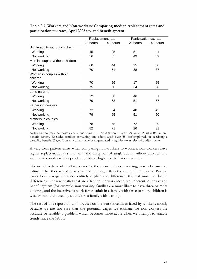
Table 2.7. Workers and Non-workers: Comparing median replacement rates and participation tax rates, April 2005 tax and benefit system
Replacement rate Participation tax rate 20 hours 40 hours 20 hours 40 hours
Single adults without children Working 45 25 51 41 Not working 56 35 49 39
Men in couples without children Working 60 44 25 30 Not working 70 51 38 37
Women in couples without children
Working 70 56 17 25 Not working 75 60 24 28
Lone parents
Working 72 58 46 51 Not working 79 68 51 57
Fathers in couples Working 72 54 48 45 Not working 79 65 51 50
Mothers in couples Working 78 65 72 29 Not working 82 71 26 31
Notes and sources: Authors’ calculations using FRS 2002–03 and TAXBEN under April 2005 tax and benefit system. Excludes families containing any adults aged over 55, self-employed, or receiving a disability benefit. Wages for non-workers have been generated using Heckman selectivity adjustments. A very clear pattern exists when comparing non-workers to workers: non-workers have higher replacement rates and, with the exception of single adults without children and women in couples with dependent children, higher participation tax rates.
The incentive to work at all is weaker for those currently not working, mostly because we estimate that they would earn lower hourly wages than those currently in work. But the lower hourly wage does not entirely explain the difference: the rest must be due to differences in characteristics that are affecting the work incentives inherent in the tax and benefit system (for example, non-working families are more likely to have three or more children, and the incentive to work for an adult in a family with three or more children is weaker than that faced by an adult in a family with 1 child).
The rest of this report, though, focuses on the work incentives faced by workers, mostly because we are not sure that the potential wages we estimate for non-workers are accurate or reliable, a problem which becomes more acute when we attempt to analyse trends since the 1970s.
28

3. Work incentives over time Section 2.4 looked at the distribution of financial work incentives in 2005-06 and examined which sorts of people face the strongest and weakest incentives to work at all and to progress. This chapter examines how these incentives have changed since 1979. It looks at changes in both the incentive to work at all, captured by the participation tax rate and the replacement rate, and the incentive to progress in the labour market, as captured by the EMTR.
As well as showing the main trends, we also explain what has caused these changes. First, we show how the changes are split between high-level demographic groups (defined by whether they live with a partner, whether they have children, and, for those people who live with a partner, by gender). Second, we show how much of the changes can be explained by various factors, such as changes to the tax and benefit system, changes in the real level of wages and their distribution, and changes to the real level of rents; the precise methodology is explained in Box 3.1.
We focus on the work incentives faced by workers. We use data from the Family Expenditure Survey (FES) for the years 1979 to 1993, and the Family Resources Survey (FRS) thereafter.17
3.1 What has happened to financial work incentives on average?
Understanding the Figures in this chapter.
Many figures in chapter 3 show five series over time: the 10th, 25th, 50th, 75th and 90th centiles of the distribution of work incentives within a particular group of the population. The 10th and 25th centiles illustrate the financial work incentives of people with relatively strong financial work incentives, and the 75th and 90th centiles illustrate the incentives of people with relatively weak financial work incentives.
Years on the horizontal axis of the Figures refer to calendar years until 1993, and then financial years.
We usually measure incentives to work at all at a fixed number of hours a week (either 20 or 40) in order that changes over time in weekly hours worked do not affect our results.
EMTRs have been calculated by increasing observed hours worked by 5% (so around 1 hour a week for a part-time worker, and 2 hours a week for a full-time worker).
17 The FES records cohabiting couples as being single individuals before 1990. We therefore impute cohabitation status for these years. The movement from imputed to actual cohabitation status in 1990 may help explain the slight discontinuity that is seen in some of our aggregate series. At the time this analysis was undertaken, the latest data was FRS 2002/3, and analysis for later years was based on uprated 2002/3 data.
29

The incentive to work at all
The financial incentive to work at all, as captured by both the participation tax rate and the replacement rate, has generally strengthened (ie the rates have fallen) between 1979 and 2005. Figure 3.1 shows what has happened to replacement rates, and Figure 3.2 shows the same for participation tax rates amongst all working individuals, evaluated at their usual hours of work (Box 3.1 gives more detail on the methodology used to construct that Figure and others in this chapter).
The changes have not been even, though, across the period. Replacement rates rose in the early 1980s, before falling over the rest of the decade (recall that replacement rates fall when financial work incentives strengthen). The turn of the 1990s saw the incentive to work at all weaken briefly, before a long period through the 1990s of relatively small changes, with mostly strengthening incentives. Work incentives in 2005 are slightly stronger than they were in 1997.
The changes in replacement rates have been uneven across the distribution: there has been a tendency for the distribution of replacement rates at a point in time to become more dispersed: the 90:10 ratio has grown from 3.2 to 4.3 over the period. The increased dispersion has arisen because the weakest incentives to work at all have not changed, or have weakened, over time, but the strongest incentives to work have become stronger.
The median participation tax rate has generally shown the same trend as the median replacement rate, and shows more pronounced changes. Changes across the distribution are rather different, with the participation tax rate showing reduced (rather than increased) dispersion over time. This difference is not enormously meaningful in itself: PTRs and RRs are constructed in different ways, and there is no reason to expect their variances to be related. But it suggests that whether the weakest incentives have strengthened relative to the strongest incentives is ambiguous, depending on which measure of incentives is used.
It is worth repeating the key conclusions because they will be echoed when we examine the changes amongst different sub-groups. In particular, incentives to work at all generally:
• are stronger in 2005 than in 1979, on average
• weakened in the early 1980s, at the turn of the 1990s, and in the early 2000s
• weakened over most of the 1980s and over most of the 1990s
• got more dispersed over time when measured by the replacement rate, but less dispersed when measured by the participation tax rate.
30

Figure 3.1. Replacement rates: 1979 - 2005
10
20
30
40
50
60
70
80
90
1979
1981
1983
1985
1987
1989
1991
1993
1995
1997
1999
2001
2003
2005
Year
Mea
n In
cent
ive
Rat
e (%
)
Notes and sources: Authors’ calculations using various years of FES/FRS and TAXBEN. Excludes families containing any adults aged over 55, the self-employed, or adults receiving a disability benefit.. Replacement rates evaluated at usual hours worked. Figure shows, from bottom to top, the changes in the 10th, 25th, 50th, 75th and 90th centiles of the distribution.
Figure 3.2. Participation tax rates: 1979 - 2005
0
10
20
30
40
50
60
70
80
1979
1981
1983
1985
1987
1989
1991
1993
1995
1997
1999
2001
2003
2005
Year
Mea
n In
cent
ive
Rat
e (%
)
Notes and sources: Authors’ calculations using various years of FES/FRS and TAXBEN. Excludes families containing any adults aged over 55, the self-employed, or adults receiving a disability benefit. Replacement rates evaluated at usual hours worked. Figure shows, from bottom to top, the changes in the 10th, 25th, 50th, 75th and 90th centiles of the distribution.
31
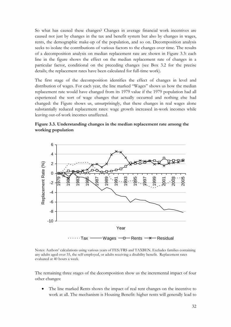
So what has caused these changes? Changes in average financial work incentives are caused not just by changes in the tax and benefit system but also by changes in wages, rents, the demographic make-up of the population, and so on. Decomposition analysis seeks to isolate the contributions of various factors to the changes over time. The results of a decomposition analysis on median replacement rate are shown in Figure 3.3: each line in the figure shows the effect on the median replacement rate of changes in a particular factor, conditional on the preceding changes (see Box 3.2 for the precise details; the replacement rates have been calculated for full-time work).
The first stage of the decomposition identifies the effect of changes in level and distribution of wages. For each year, the line marked “Wages” shows us how the median replacement rate would have changed from its 1979 value if the 1979 population had all experienced the sort of wage changes that actually occurred and nothing else had changed: the Figure shows us, unsurprisingly, that these changes in real wages alone substantially reduced replacement rates: wage growth increased in-work incomes while leaving out-of-work incomes unaffected.
Figure 3.3. Understanding changes in the median replacement rate among the working population
-10
-8
-6
-4
-2
0
2
4
6
1979
1981
1983
1985
1987
1989
1991
1993
1995
1997
1999
2001
2003
2005
Year
Rep
lace
men
t Rat
e (%
)
Tax Wages Rents Residual
Notes: Authors’ calculations using various years of FES/FRS and TAXBEN. Excludes families containing any adults aged over 55, the self-employed, or adults receiving a disability benefit. Replacement rates evaluated at 40 hours a week.
The remaining three stages of the decomposition show us the incremental impact of four other changes:
• The line marked Rents shows the impact of real rent changes on the incentive to work at all. The mechanism is Housing Benefit: higher rents will generally lead to
32

higher entitlements to Housing Benefit, which increases out-of-work income and increases in-work income by the same or a smaller amount. The Figure confirms that real rent changes weakened the incentive to work at all.
• The line marked Tax shows the impact of real tax and benefit changes. It shows that the tax and benefit systems between 1980 and 1989 led to weaker incentives to work than in 1979, because the line marked “Tax” is above the zero line, but that those after 1989 would have led to stronger incentives to work compared with 1979). It also shows that the impact of real tax and benefit changes since 1999 has been to weaken the median incentive to work.
• Lastly, the residual shows the incremental changes caused by all other changes (see Box 3.2 for what this might include).
It is important to recognise that decompositions have limitations. They aim to isolate the effect of policy changes (for example) by showing what work incentives would have looked like in the absence of policy changes, holding all other factors constant. But “holding other factors constant” is problematic in two respects:
• in practice people may well have behaved differently, changing these “other factors”, if different policies had been in place. So this decomposition approach can only identify the direct effect of policy: it cannot tell us, for example, how far tax and benefit reforms changed work incentives by affecting the wages offered by employers.
• the decomposition treats changes sequentially, whereas they actually occurred simultaneously. Thus the estimated impacts from the decomposition analysis are order-dependent: each stage identifies the additional effect of a particular change, conditional on the preceding changes, so the effect of each factor might vary according to whether other factors are held constant at their 1979 or 2000 levels.
As Box 3.2 makes clear, the results from this sort of analysis are order-dependent: each stage identifies the additional effect of a particular change, conditional on the preceding changes. In work not shown here we performed the decompositions in a different order.18 Reassuringly, the results are not quantitatively identical, but are qualitatively similar:
• real wage changes have always strengthened the incentive to work at all.
• The tax and benefit systems in operation between 1980 and 1989 all led to weaker incentives to work at all than that of 1979; those since 1989 led to stronger incentives. Real tax and benefit changes since 1999, though, have been weakening the incentive to work at all.
• increased real rents and all other changes have all weakened the incentive to work.
18 The order of the alternative decomposition was: real tax and benefit changes, average wage growth, wage inequality, real rent changes, all other changes.
33

Results for all of the decomposition shown in this paper are available performed in this other order, and we report them here only when they are of interest. Generally, the order of the decomposition can matter, particularly in the most recent years, when deciding how much of the observed change in financial incentives is due to changes in wages, and how much is due to changes in the tax and benefit system. For example, whether the tax and benefit system in 2005–06 leads to stronger or weaker incentives to progress (on average) than the one in 1979 depends on whether we calculate incentives in 2005–06 using the real wages observed in 1979 or in 2005–06.
34

Box 3.2. Understanding the changes in financial work incentives though a decomposition analysis
The main technique used in our work to understand the changes in financial work incentives is to decompose the observed changes into those caused by changes to the tax and benefit system, and those due to changes in the characteristics of the working population.
To do this, we start with the population observed in 1979 facing the tax and benefit system of 1979. We then change economic variables and characteristics of this population until we end up with the actual population in a different year (say 2000), with the actual tax and benefit system of 2000. 19 The stages in the decomposition are described below, assuming for simplicity that we are only comparing 1979 and 2000 (in reality we do this for every year):
1. Identify the contribution of changes in the level and distribution of wages, by assuming that the population in 2000 has the same real characteristics as in 1979 except for wages, which follow the distribution of the 2000 population. We do this by projecting the actual wage distribution in 2000 onto the 1979 population, so that each 1979 individual is assigned the wage of someone observed in 2000 with the same wage ranking within the relevant demographic group. Comparing the work incentives of this wage-adjusted 1979 population with those of the actual 1979 population, both under the 1979 tax and benefit system, shows the impact of wage changes alone on work incentives.
2. Identify the additional contribution of real changes in average rents (but still assuming that the proportion of the group in rented accommodation is the same as 1979) by increasing all rents by the growth in average rents between 1979 and 2000.
3. Identify the additional contribution of real changes to the tax and benefit system by allowing the tax and benefit system to change. 20
4. Identify the additional contribution of all other changes that might affect financial work incentives, such as changes in non-earned income, housing tenure, disability and ill health, and, amongst parents, the number and age of dependent children. This also includes changes in the working patterns amongst couples: as shown in chapter 2, this will be an important factor in explaining financial work incentives amongst individuals in couples.
19 Similar analyses have been undertaken by, for example, Adam and Brewer (2004) to explain changes in child-contingent support, and Dickens and Ellwood (2004) to explain changes in child poverty in the US and UK.
20 When looking at changes over this long period (25 years), it is arguably more sensible to assume that the appropriate index for uprating tax and benefit parameters over time should be the growth in average earnings rather than the growth in average retail prices (see Clark and Leicester (2004), Evans and Eyre (2004)). However, we have decided to assume that “no real changes” is the baseline, but to show the impact of real changes in the tax and benefit system separately from the impact of real changes in wages.
35

Later sections in this chapter give more detail of how financial work incentives have changed for particular groups.
The incentive to progress
Trends in the financial incentive to progress – as measured by EMTRs – are shown in Figure 3.4.
The economy-wide median incentive shows a similar pattern to the incentive to work at all. It weakened in the early 1980s, and strengthened rapidly between 1985 and 1988. Between 1988 and 1995, it weakened slightly, then strengthened between 1995 and 1997, since when it has been weakening once more.
However, the trend shown by the other lines on the Figure is rather different from the median. The distribution of incentives to progress has become much more dispersed over time: in 1979, 80% of the population faced EMTRs of between 29% and 37%; in 2004–05, the range is between 23% and 68%. 21 This increased dispersion is less evident when examining the inter-quartile range (the 25th and 75th centiles): it is due to changes for those with the strongest and weakest incentives. In particular, the strongest incentives to progress (measured by the 10th centile) have strengthened by more than the median, particularly between 1995 and 2000, when tax rates for low earners were being cut, and the weakest incentives to progress (measured by the 90th centile) have got a lot weaker since 1999, as eligibility for in-work support extended both up the income distribution and (in 2003) to people without children.
Figure 3.4 also shows us that, Since 2003, more than one in four workers have faced an effective marginal tax rate of around 40 per cent or more, the first time this has happened since 1985. This reflects both the impact of fiscal drag on the number of higher-rate taxpayers and the increasing numbers of workers entitled to in-work support.22
21 This is taking the 80% of the population who are not at the extremes of the distribution: those lying between the 10th and 90th centiles.
22 People rich enough to pay higher-rate tax but who are contracted out of the state second pension would face an EMTR of 39.4% after April 2003 (we ignore the additional age-related NICs rebate that applies to people who are contracted out into defined contribution pension schemes).
36

Figure 3.4. Effective marginal tax rates: 1979 – 2005
20
30
40
50
60
70
1979
1981
1983
1985
1987
1989
1991
1993
1995
1997
1999
2001
2003
2005
Year
Mar
gina
l Effe
ctiv
e Ta
x R
ate
(%)
Notes and sources: Authors’ calculations using various years of FES/FRS and TAXBEN. Excludes families containing any adults aged over 55, the self-employed, or adults receiving a disability benefit. Replacement rates evaluated at usual hours worked. Figure shows, from bottom to top, the changes in the 10th, 25th, 50th, 75th and 90th centiles of the distribution.
Changes in the median incentive to progress are overwhelmingly determined by changes to the tax and benefit system: the decline in the median EMTR during the mid 1990s reflects the successive cuts in the basic rate of income tax, for example. For this reason, we instead show a decomposition of changes in the mean EMTR in Figure 3.5. The key results are:
• real tax and benefit changes are the single most important determinant of changes in the average incentive to progress.
• The tax and benefit systems between 1980 and 1987 produced weaker incentives to progress, on average, than that of 1979; those more recent than 1988 have produced stronger incentives to progress, on average. But the impact of recent tax and benefit changes (since 1999) has been to weaken, on average, incentives to progress, raising the average EMTR by almost 3 percentage points.23
23 Whether the tax and benefit system in 2005–06 leads to stronger or weaker incentives to progress (on average) than the one in 1979 depends on whether we calculate incentives in 2005–06 using the real earnings observed in 1979 or in 2005/06. In work not shown here, we find that if real wages had not changed since 1979, then real tax and benefit reforms between 1979 and 2005 would have reduced average incentives to progress, because of the increased support for low-income working families, and the consequential increased likelihood that workers would face a withdrawal of income-related support as their earning rise. However, once we allow for real wages to grow, then real tax and benefit reforms between 1979 and 2005 have strengthened average incentives to progress.
37

• Over the whole period, changes in wages had very little net effect on the average incentive to progress, only slightly weakening it overall: in the first third of the period, these changes lowered the mean EMTR, but since the late 1980s they have raised it. Growth in real wages will strengthen incentives to progress for adults who become too rich to quality for means-tested benefits or tax credits, or too rich to pay National Insurance contributions on their extra earnings, but weaken them for those who move onto higher income tax rates; our analysis suggests, therefore, that the latter effect slightly outweighs the former over this whole period.
• Changes in the real level of rents, and all other changes not explicitly mentioned here, have both tended to weaken incentives to progress, on average.
Figure 3.5. Understanding changes in the mean EMTR amongst the working population
-4
-3
-2
-1
0
1
2
3
4
1979
1981
1983
1985
1987
1989
1991
1993
1995
1997
1999
2001
2003
2005
Year
EMTR
(%)
Tax Wages Rents Residual
Notes: Authors’ calculations using various years of FES/FRS and TAXBEN. Excludes families containing any adults aged over 55, the self-employed, or adults receiving a disability benefit.
Summary:
Both incentives to work at all, and incentives to progress, are generally stronger now than in 1979.
Real wage growth has greatly strengthened the incentive to work at all (measured by replacement rates), because out-of-work benefits have typically been increased only in line with price inflation, not average wage growth.
Over the whole period, changes in wages had very little effect on the average incentive to progress. Wage growth reduces EMTRs for those adults who become too rich to quality for means-tested benefits or tax credits, or too rich to pay
38

National Insurance contributions on their extra earnings, but it increases EMTRs for those who move onto higher income tax rates; our analysis suggests that these effects broadly offset each other, with the latter effect only slightly outweighing the former over this whole period.
The cumulative effect of 26 years of real tax and benefit changes has been to strengthen work incentives. The pattern has not been even, though: between 1979 and 1983, real tax and benefit changes tended to weaken the incentive to work; between 1983 and the late 1990s, they tended to strengthen it; and the most recent changes have tended to weaken it once more. Since 1999, tax and benefit changes have increased the average EMTR by almost three percentage points.
Increased real rents and all other changes have all weakened the incentive to work and incentives to progress.
3.2 How have financial work incentives changed for different groups in the population?
In the next section, we show how financial work incentives have changed for people in six different demographic groups, defined by whether they live with a partner, whether they have children, and, for those people who live with a partner, their gender. Since 1979, the relative size of these six groups has changed considerably. In work not shown here, we find that these changes hardly contribute to the trends shown in the earlier figures: instead, it is the changing financial work incentives within the six groups that have driven the changes, and so we focus on those changes below.
In each of the next sections, we echo the analysis in section 3.1: we show how the incentives to work at all and the incentives to progress have changed, and we undertake a decomposition analysis to try to understand what has been causing the changes. 24
Lone parents: incentive to work at all
As we saw in Chapter 2, lone parents face the weakest financial work incentives of our demographic groups.
The financial incentive for lone parents to work part-time (20 hours a week) is now stronger than it was in 1979, in general, as measured by replacement rates (see Figure 3.6). An important cause of the fall in three of the series shown in Figure 3.6 was the reform to family credit in 1992, when the number of hours needed to receive in-work benefits fell from 24 to 16. But there has also been a noticeable weakening of work incentives in recent years, at the same time as lone parents’ entitlements to out-of-work benefits have been rising. As for the population as a whole, replacement rates have become more dispersed over time; unlike for the population as a whole, though, the weakest incentives to work at all (the 90th centile) have been getting stronger, albeit by less than the strongest (the 10th centile). 24 When calculating replacement rates, we hold hours of work constant over time at 40 hours a week for all groups except lone parents, where we calculate incentives to work at all at 20 hours a week.
39

Our other measure of the incentive to work at all – the participation tax rate – shows broadly similar trends (Figure 3.7):
• incentives to work at all are stronger now than in 1979, with big one-off strengthenings in 1992 and 1999
• the distribution is more dispersed.
However, the PTR shows further strengthening of the incentive to work since 1999, in contrast to the RR. Indeed, the PTR shows that, since 2000, between 10 and 25 per cent of working lone parents find that their net income rises by more than their gross earnings when they move into work (this is the implication of a negative PTR, and it can happen if in-work support (less taxes) is greater than out-of-work support).
40

Figure 3.6. Changes in the part-time replacement rate amongst working lone parents, 1979 - 2005
30
40
50
60
70
80
90
100
1979
1981
1983
1985
1987
1989
1991
1993
1995
1997
1999
2001
2003
2005
Year
Rep
lace
men
t Rat
e (%
)
Notes: Authors’ calculations using various years of FES/FRS and TAXBEN. Excludes families containing any adults aged over 55, the self-employed, or adults receiving a disability benefit. Replacement rates evaluated at 20 hours. Figure shows, from bottom to top, the changes in the 10th, 25th, 50th, 75th and 90th centiles of the distribution.
Figure 3.7. Changes in the part-time PTR rate amongst working lone parents, 1979 - 2005
-40
-20
0
20
40
60
80
100
1979
1981
1983
1985
1987
1989
1991
1993
1995
1997
1999
2001
2003
2005
Year
Par
ticip
atio
n Ta
x R
ate
(%)
Notes: Authors’ calculations using various years of FES/FRS and TAXBEN. Excludes families containing any adults aged over 55, the self-employed, or adults receiving a disability benefit. Replacement rates evaluated at 20 hours. Figure shows, from bottom to top, the changes in the 10th, 25th, 50th, 75th and 90th centiles of the distribution.
41

Incentives to work full-time – not shown here – have always been stronger than those to work part-time, but have strengthened by less over this period. Non-workers – again, not shown here – have experienced similar changes in their work incentives over this same period, although, as we said in Chapter 2, their incentives are slightly weaker, in general, than those already in work.
The results of a decomposition analysis on the changes in the median replacement rate for part-time work amongst working lone parents is shown in Figure 3.8 (see Box 3.2 for the precise details). It tells us the following:
• There were only small changes to the median replacement rate between 1979 and 1991, with average wage growth tending to strengthen the incentive to work at all, but other changes weakening it
• Since 1991, real changes to the tax and benefit system have dramatically strengthened the incentive to work at all
• Changes in wages earned by lone parents has meant that incentives to work at all are stronger than they were in 1979
• Changes to rent levels, and all other changes, though, have weakened the median incentive to work at all.
According to the decomposition analysis in Figure 3.8, the weakening between 2000 and 2003 of lone parents’ incentives to work at all was not primarily due to changes in taxes and benefits: instead, the analysis suggests that it was due to the low growth in lone parents’ wages, the growth in rents, and all other changes (such as changes in lone parents’ family compositions) since 1999.
42

Figure 3.8. Understanding changes in the median part-time replacement rate amongst working lone parents
-15
-10
-5
0
5
1019
79
1981
1983
1985
1987
1989
1991
1993
1995
1997
1999
2001
2003
2005
Year
Tax Wages Rents Residual
Notes: Authors’ calculations using various years of FES/FRS and TAXBEN. Excludes families containing any adults aged over 55, the self-employed, or adults receiving a disability benefit. Replacement rates evaluated at 20 hours.
Lone parents: incentive to progress
Changes in lone parents’ incentives to progress in the labour market are shown in Figure 3.9. It shows that:
• the weakest incentives to progress have strengthened since the early 1980s: since 1999, 75 per cent of working lone parents have had an EMTR below 70%, the highest proportion since 1982. In 1999, the proportion of working lone parents with EMTRs of 100% or more fell below 10% for the first time in our data.
• The strongest incentives to progress have hardly changed (25th centile) or have slightly strengthened (10th centile) since 1979. This group represents lone parents who are unaffected by withdrawal rates in means-tested benefits or in-work support, either because they don’t have low enough incomes to be entitled or because they earn so little that extra earnings do not reduce entitlements.
• The median incentive to progress, though, has weakened over time, with the median EMTR jumping from around 40% to around 70% as entitlement to in-work support has grown amongst working lone parents.
43

Figure 3.9. Effective marginal tax rates for working lone parents: 1979 - 2005
0
20
40
60
80
100
1979
1981
1983
1985
1987
1989
1991
1993
1995
1997
1999
2001
2003
2005
Year
Mar
gina
l Effe
ctiv
e Ta
x R
ate
(%)
Notes: Authors’ calculations using various years of FES/FRS and TAXBEN. Excludes families containing any adults aged over 55, the self-employed, or adults receiving a disability benefit. Figure shows, from bottom to top, the changes in the 10th, 25th, 50th, 75th and 90th centiles of the distribution.
As with the population as a whole, changes in the median EMTR track changes in the tax and benefit system. The results of a decomposition analysis of the mean incentive to progress are shown in Figure 3.10. As with other Figures showing changes in lone parents’ work incentives, some of the individual series (particularly the “residual”, or the impact of all changes not explicitly accounted for) are rather volatile. The key results are the following:
• real tax and benefit changes have weakened incentives to progress from their 1979 level particularly because of reforms in the early 1990s.
• Changes in the wages received by lone parents strengthened their incentives to progress, particularly after 1988, presumably by making fewer of them eligible to means-tested benefits or tax credits.
• Changes in the real level of rents have weakened incentives to progress, by extending the range of earnings consistent with eligibility to housing benefit.
44

Figure 3.10. Understanding changes in the mean EMTR amongst working lone parents
-15
-10
-5
0
5
10
15
2019
79
1981
1983
1985
1987
1989
1991
1993
1995
1997
1999
2001
2003
2005
Year
Tax Wages Rents Residual
Notes: Authors’ calculations using various years of FES/FRS and TAXBEN. Excludes families containing any adults aged over 55, the self-employed, or adults receiving a disability benefit.
Summary:
The incentive for lone parents to work part-time (compared to not working) is generally stronger now than in 1979, both because real wages have risen and because in-work support is now available for part-time as well as full-time workers. On the other hand, real rent rises and housing benefit have weakened the incentive for lone parents to work, and incentives to work in 2005 are slightly weaker than they were in 1999.
Until the early 1990s, the extension of in-work support amongst lone parents was broadly in line with the real changes in lone parents’ wages, and so incentives to progress were broadly unchanged from their 1979 level. Reforms to family credit in the early 1990s, though, extended in-work support to many more lone parents, weakening incentives to progress, on average, for those already in work. In more recent years, the expansion of tax credits has increased EMTRs for relatively well-off lone parents previously facing strong incentives to progress, but strengthened some of the weakest incentives to progress. But it is still the case in 2005–06 that more than half of working lone parents would, once the temporary disregard in tax credits had expired, keep less than a third of any extra earnings if they worked an hour or two more each week.
45

Couples with children: incentive to work at all
The incentive for men in couples with children to work full-time generally weakened in the early 1980s, strengthened slowly from the mid 1980s to the late 1990s, but has begun to weaken since then (see Figures 3.11 and 3.12).
As in the whole population, there has been a slight increase over time in the dispersion of RRs, but a reduction in the dispersion of PTRs. Comparing 1979 and 2005, there has been little change in the highest RRs, but a reduction in the lowest; there has been little change in the lowest PTRs, but a reduction in the highest. This is the only demographic group for whom the dispersion of PTRs has narrowed.
Figure 3.11. Changes in the full-time replacement rate amongst working fathers in couples, 1979 - 2005
0
10
20
30
40
50
60
70
80
90
1979
1981
1983
1985
1987
1989
1991
1993
1995
1997
1999
2001
2003
2005
Year
Rep
lace
men
t Rat
e (%
)
Notes: Authors’ calculations using various years of FES/FRS and TAXBEN. Excludes families containing any adults aged over 55, the self-employed, or adults receiving a disability benefit. Replacement rates evaluated at 40 hours. Figure shows, from bottom to top, the changes in the 10th, 25th, 50th, 75th and 90th centiles of the distribution.
46

Figure 3.12. Changes in the full-time PTR amongst working fathers in couples, 1979 - 2005
0
10
20
30
40
50
60
70
80
9019
79
1981
1983
1985
1987
1989
1991
1993
1995
1997
1999
2001
2003
2005
Year
Par
ticip
atio
n Ta
x R
ate
(%)
Notes: Authors’ calculations using various years of FES/FRS and TAXBEN. Excludes families containing any adults aged over 55, the self-employed, or adults receiving a disability benefit. Rates evaluated at 40 hours. Figure shows, from bottom to top, the changes in the 10th, 25th, 50th, 75th and 90th centiles of the distribution.
Financial incentives to work at all tend to be weaker amongst working mothers in couples than fathers in couples, and the distribution is much less dispersed (Figures 3.13 and 3.14). For the majority of women in couples, the trends are broadly similar to those amongst fathers in couples – a gradual strengthening from the early 1980s to the late 1990s, with spells of weakening incentives before and after this period. Unlike for men, though, the weakest incentives faced by women became weaker even between the early 1980s and the late 1990s. As for men, there has been an increase in the dispersion of RRs; but unlike for men, the dispersion of PTRs has also increased.
The part-time replacement rate amongst working mothers in couples tends to be higher than the full-time replacement rate, but the trend over this period is extremely similar (not shown).
47

Figure 3.13. Changes in the full-time replacement rate amongst working mothers in couples, 1979 - 2005
20
30
40
50
60
70
80
90
1979
1981
1983
1985
1987
1989
1991
1993
1995
1997
1999
2001
2003
2005
Year
Rep
lace
men
t Rat
e (%
)
Notes: Authors’ calculations using various years of FES/FRS and TAXBEN. Excludes families containing any adults aged over 55, the self-employed, or adults receiving a disability benefit. Rates evaluated at 40 hours. Figure shows, from bottom to top, the changes in the 10th, 25th, 50th, 75th and 90th centiles of the distribution.
48

Figure 3.14. Changes in the full-time PTR amongst working mothers in couples, 1979 - 2005
0
10
20
30
40
50
60
70
80
9019
79
1981
1983
1985
1987
1989
1991
1993
1995
1997
1999
2001
2003
2005
Year
Par
ticip
atio
n Ta
x R
ate
(%)
Notes: Authors’ calculations using various years of FES/FRS and TAXBEN. Excludes families containing any adults aged over 55, the self-employed, or adults receiving a disability benefit. Rates evaluated at 40 hours. Figure shows, from bottom to top, the changes in the 10th, 25th, 50th, 75th and 90th centiles of the distribution.
Decomposing the changes in the median full-time RR for fathers in couples suggests the following (see Figure 3.15):
• Real tax and benefit changes have tended to weaken the incentive to work at all, with particularly marked deteriorations in the early 1980s and since the late 1990s.
• Changes in the wages earned by men in couples with children has more than offset this, though, substantially strengthening the incentive to work at all.
• Real growth in rents has slightly increased the median replacement rate.
Although the changes are much less pronounced, the same decomposition for women in couples with dependent children (Figure 3.16) tells the same story: real tax and benefit changes alone would have weakened the median incentive to work at all, but changes in the wages received by these women have more than offset this.
49

Figure 3.15 Understanding changes in the median full-time replacement rate amongst working fathers in couples
-12-10
-8-6-4-202468
1979
1981
1983
1985
1987
1989
1991
1993
1995
1997
1999
2001
2003
2005
Year
Tax Wages Rents Residual
Notes: Authors’ calculations using various years of FES/FRS and TAXBEN. Excludes families containing any adults aged over 55, the self-employed, or adults receiving a disability benefit. Rates evaluated at 40 hours.
Figure 3.16 Understanding changes in the median full-time replacement rate amongst working mothers in couples
-12-10-8-6-4-202468
1979
1981
1983
1985
1987
1989
1991
1993
1995
1997
1999
2001
2003
2005
Year
Tax Wages Rents Residual
Notes: Authors’ calculations using various years of FES/FRS and TAXBEN. Excludes families containing any adults aged over 55, the self-employed, or adults receiving a disability benefit. Rates evaluated at 40 hours.
50
Couples with children: incentive to progress
Trends in the incentives to progress facing working fathers in couples are shown in Figure 3.17. Between 1979 and 1999, the trends are very similar across the distribution of working fathers, and very similar to those of the general population. Incentives to progress have been weakening since 1999 at most points in the distribution; the marked jump in the 90th centile shows us that, after WFTC was introduced, more than 10 per cent of working fathers were in families receiving in-work support.
The trend in the median EMTR for working mothers in couples (Figure 3.18) is very similar to that for working fathers. The other lines, though, look quite different. This is partly because, over much of our period, a significant minority of working mothers faced either zero, or a very low, EMTR. Typically, these are women with income below the personal allowance and so not paying income tax, but whose partners have a high enough income that the family is not entitled to in-work support.
51
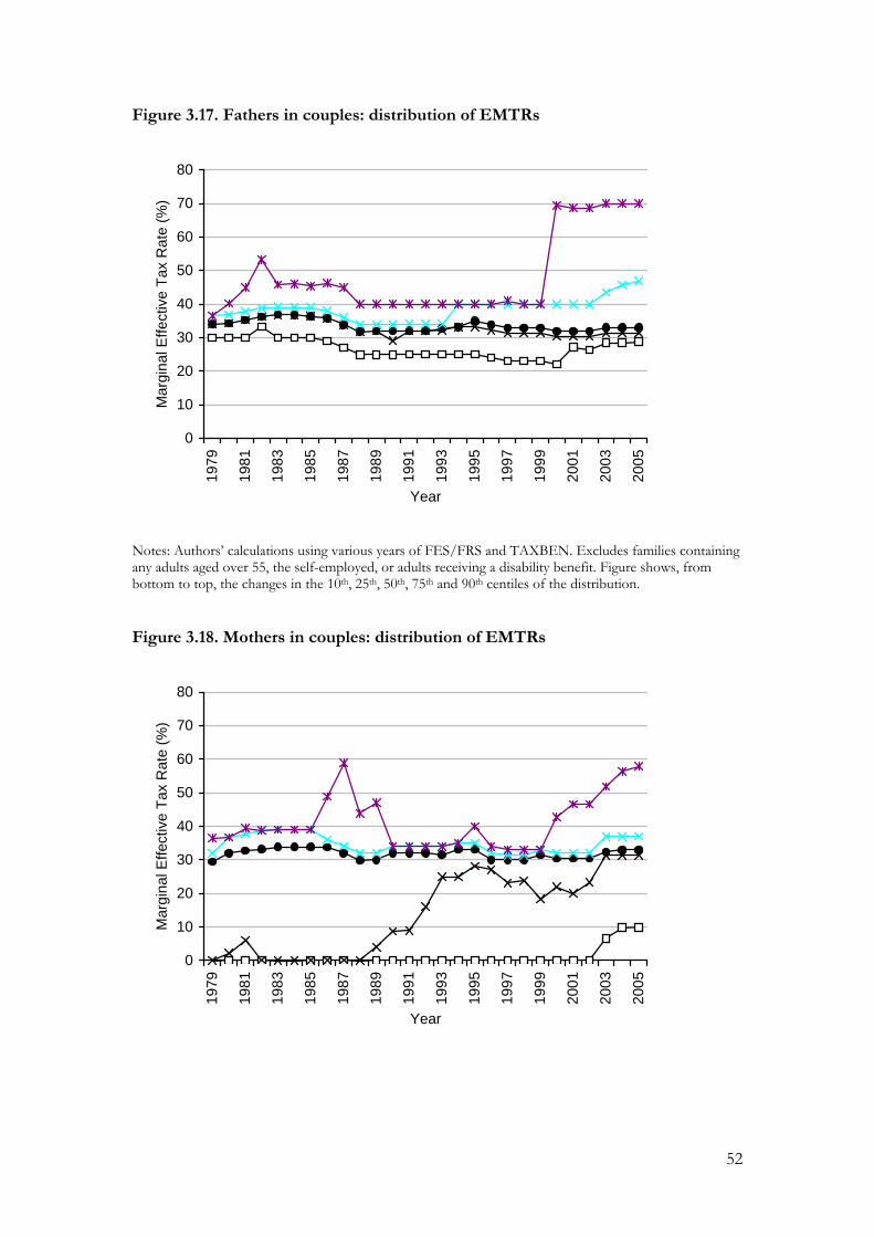
Figure 3.17. Fathers in couples: distribution of EMTRs
0
10
20
30
40
50
60
70
80
1979
1981
1983
1985
1987
1989
1991
1993
1995
1997
1999
2001
2003
2005
Year
Mar
gina
l Effe
ctiv
e Ta
x R
ate
(%)
Notes: Authors’ calculations using various years of FES/FRS and TAXBEN. Excludes families containing any adults aged over 55, the self-employed, or adults receiving a disability benefit. Figure shows, from bottom to top, the changes in the 10th, 25th, 50th, 75th and 90th centiles of the distribution.
Figure 3.18. Mothers in couples: distribution of EMTRs
0
10
20
30
40
50
60
70
80
1979
1981
1983
1985
1987
1989
1991
1993
1995
1997
1999
2001
2003
2005
Year
Mar
gina
l Effe
ctiv
e Ta
x R
ate
(%)
52

Notes: Authors’ calculations using various years of FES/FRS and TAXBEN. Excludes families containing any adults aged over 55, the self-employed, or adults receiving a disability benefit. Figure shows, from bottom to top, the changes in the 10th, 25th, 50th, 75th and 90th centiles of the distribution.
The results of decomposition analyses of the mean incentive to progress are shown in Figure 3.19 and 3.20. The key results are the following:
• the tax and benefit systems between 1980 and 1987 produced weaker incentives to progress, on average, than that of 1979; those between 1988 and 1998 produced stronger incentives to progress, on average, for both fathers and mothers, than in 1979. The impact of tax and benefit changes since the second half of the 1990s has been to weaken, on average, incentives to progress. For fathers, the combined effect of real tax and benefit changes over the whole period has been to weaken incentives to progress compared to 1979; for mothers, it has been to strengthen them.
• Changes in the wages received by men in couples with dependent children have had little impact, on average, on their incentives to progress; amongst women in couples with dependent children, though, such changes have weakened incentives to progress, presumably because more of these women are now earning enough to pay income tax.
• Rises in the real level of rents have had small but negative impacts on incentives to progress, by extending the range of earnings consistent with eligibility to housing benefit.
53
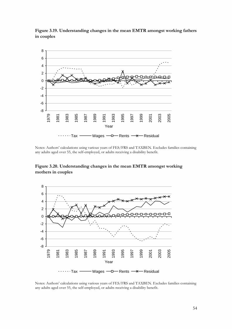
Figure 3.19. Understanding changes in the mean EMTR amongst working fathers in couples
-8
-6
-4
-2
0
2
4
6
819
79
1981
1983
1985
1987
1989
1991
1993
1995
1997
1999
2001
2003
2005
Year
Tax Wages Rents Residual
Notes: Authors’ calculations using various years of FES/FRS and TAXBEN. Excludes families containing any adults aged over 55, the self-employed, or adults receiving a disability benefit.
Figure 3.20. Understanding changes in the mean EMTR amongst working mothers in couples
-8
-6
-4
-2
0
2
4
6
8
1979
1981
1983
1985
1987
1989
1991
1993
1995
1997
1999
2001
2003
2005
Year
Tax Wages Rents Residual
Notes: Authors’ calculations using various years of FES/FRS and TAXBEN. Excludes families containing any adults aged over 55, the self-employed, or adults receiving a disability benefit.
54

Summary:
Growth in real earnings led to a gradual strengthening of the incentive to be in work for men and women in couples with children from the early 1980s to the late 1990s, but tax and benefit changes weakened incentives to work both before and after this period.
Higher earnings amongst working mothers has meant that more of them now pay income tax than in 1979, dulling incentives to progress. Aside from this, the main change to incentives to progress for adults in couples with children took place since the late 1990s, with the expansion of in-work support weakening incentives to progress for a minority.
Single people without children: incentive to work at all
As chapter 2 showed, single people without children have the strongest incentives to work at all, on average, because they would be entitled to little income from benefits if they did not work. Indeed, the replacement rates of single individuals without children with relatively weak incentives to work are very similar to those of lone parents with relatively strong incentives.
Since the early 1980s, replacement rates and participation tax rates for full-time work for single people without children have declined almost continuously, with the median replacement rate falling by 6 percentage points over the entire period (Figure 3.21). Not all the population has experienced the same strengthening: those with the weakest incentives have generally seen the least strengthening.25 Between the mid 1990s and 2003, PTRs rose but RRs continued to fall (Figure 3.22).
25 Part-time replacement rates for single people without children are higher than those for full-time work (about 20 percentage points at the median) and the distribution is more dispersed. However, the trends are very similar to those for full-time work. Financial work incentives for non-workers are weaker than those for workers: the median replacement rate is around 5 percentage points higher. Over time, financial work incentives for non-working single people without children have changed little at the median, and have weakened at the 75th percentile point, with strengthening only at the 25th percentile, amongst those with already relatively strong financial work incentives.
55

Figure 3.21. Changes in the full-time replacement rate amongst working single people without children, 1979 - 2005
10
20
30
40
50
60
70
1979
1981
1983
1985
1987
1989
1991
1993
1995
1997
1999
2001
2003
2005
Year
Rep
lace
men
t Rat
e (%
)
Notes: Authors’ calculations using various years of FES/FRS and TAXBEN. Excludes families containing any adults aged over 55, the self-employed, or adults receiving a disability benefit. Rates evaluated at 40 hours. Figure shows, from bottom to top, the changes in the 10th, 25th, 50th, 75th and 90th centiles of the distribution.
56

Figure 3.22. Changes in the full-time PTR amongst working single people without children, 1979 - 2005
0
10
20
30
40
50
60
70
80
9019
79
1981
1983
1985
1987
1989
1991
1993
1995
1997
1999
2001
2003
2005
Year
Par
ticip
atio
n Ta
x R
ate
(%)
Notes: Authors’ calculations using various years of FES/FRS and TAXBEN. Excludes families containing any adults aged over 55, the self-employed, or adults receiving a disability benefit. Rates evaluated at 40 hours. Figure shows, from bottom to top, the changes in the 10th, 25th, 50th, 75th and 90th centiles of the distribution.
The decomposition analysis, shown in Figure 3.23, suggests the following:
• As for the population as a whole, the tax and benefit systems between 1980 and 1989 led to weaker average incentives to work at all than that of 1979; those since 1989 have led to stronger incentives.
• This change, though, is much smaller than the strengthening caused by changes in wages received by single adults without children.
• Real growth in rents and all other changes have weakened incentives to work at all.
57

Figure 3.23. Understanding changes in the median full-time replacement rate amongst working single people without children
-10
-8
-6
-4
-2
0
2
4
6
1979
1981
1983
1985
1987
1989
1991
1993
1995
1997
1999
2001
2003
2005
Year
Rep
lace
men
t Rat
e (%
)
Tax Wages Rents Residual
Notes: Authors’ calculations using various years of FES/FRS and TAXBEN. Excludes families containing any adults aged over 55, the self-employed, or adults receiving a disability benefit. Rates evaluated at 40 hours.
Single people without children: incentive to progress
Figure 3.24 shows the changes in the financial incentives to progress facing single adults. The general trend is familiar: incentives strengthened between the early 1980s and the late 1990s, but got weaker outside this period. There is also increasing dispersion of incentives over time.
58

Figure 3.24. Singles people without children: distribution of EMTRs
20
25
30
35
40
45
50
1979
1981
1983
1985
1987
1989
1991
1993
1995
1997
1999
2001
2003
2005
Year
Mar
gina
l Effe
ctiv
e Ta
x R
ate
(%)
Notes: Authors’ calculations using various years of FES/FRS and TAXBEN. Excludes families containing any adults aged over 55, the self-employed, or adults receiving a disability benefit. Figure shows, from bottom to top, the changes in the 10th, 25th, 50th, 75th and 90th centiles of the distribution.
A decomposition analysis (Figure 3.25) shows that:
• the tax and benefit systems between 1980 and 1987 led to weaker incentives to progress than that of 1979; those since 1987 have led to stronger incentives. However, changes since 2002 have been weakening average incentives to progress.
• Increases in wages have slightly strengthened incentives to progress, but real growth in rents and all other changes have weakened incentives to progress.
59

Figure 3.25. Understanding changes in the mean EMTR amongst working single adults without children
-5
-4
-3
-2
-1
0
1
2
3
419
79
1981
1983
1985
1987
1989
1991
1993
1995
1997
1999
2001
2003
2005
Year
Tax Wages Rents Residual
Notes: Authors’ calculations using various years of FES/FRS and TAXBEN. Excludes families containing any adults aged over 55, the self-employed, or adults receiving a disability benefit.
Summary:
Single adults without children faced relatively strong incentives to work even in 1979. Real wage growth since then has strengthened this further, as have tax and benefit changes.
Incentives to progress strengthened for most of the period, but weakened in the early 1980s, and have been weakening since the late 1990s: these changes are driven by real tax and benefit changes.
Couples without children: incentive to work at all
Over time, incentives for working men in couples without children to work full-time have changed in a similar way to those for single people without children (see Figures 3.26 and 3.27). Incentives to work at all tended to weaken between 1979 and 1986, strengthen between 1986 and the late 1990s, and have slightly weakened in recent years. As with most other groups examined so far, the dispersion of incentives to work at all has widened: the weakest incentives have strengthened by less than the strongest.
Over the same period, the median replacement rate for working women in couples without children has also fallen, by around 5 percentage points (Figure 3.28). This reduction is very similar in magnitude to that experienced by working men in couples without children, but the declines took place at different points in time: for men, much of the reduction occurred between the mid 1980s and the early 1990s; for women, the reduction began in the early 1990s. As with men, we see increasing dispersion over time,
60

although the distribution of RRs is less dispersed than for men. Trends in PTRs (Figure 3.29) are broadly the same, although the weakening at the start and the end of the whole period is more noticeable than with the RR. 26
26 The replacement rates of non-workers in couples without children (not shown here) has changed by little since 1979, with strengthening of financial work incentives limited to women in the most recent few years.
61

Figure 3.26 Changes in the full-time replacement rate amongst working men in couples without children, 1979 - 2005
20
30
40
50
60
70
80
1979
1981
1983
1985
1987
1989
1991
1993
1995
1997
1999
2001
2003
2005
Year
Rep
lace
men
t Rat
e (%
)
Notes: Authors’ calculations using various years of FES/FRS and TAXBEN. Excludes families containing any adults aged over 55, the self-employed, or adults receiving a disability benefit. Figure shows, from bottom to top, the changes in the 10th, 25th, 50th, 75th and 90th centiles of the distribution.
Figure 3.27. Changes in the full-time PTR amongst working men in couples without children, 1979 - 2005
0
10
20
30
40
50
60
70
80
90
1979
1981
1983
1985
1987
1989
1991
1993
1995
1997
1999
2001
2003
2005
Year
Par
ticip
atio
n Ta
x R
ate
(%)
Notes: Authors’ calculations using various years of FES/FRS and TAXBEN. Excludes families containing any adults aged over 55, the self-employed, or adults receiving a disability benefit. Figure shows, from bottom to top, the changes in the 10th, 25th, 50th, 75th and 90th centiles of the distribution.
62
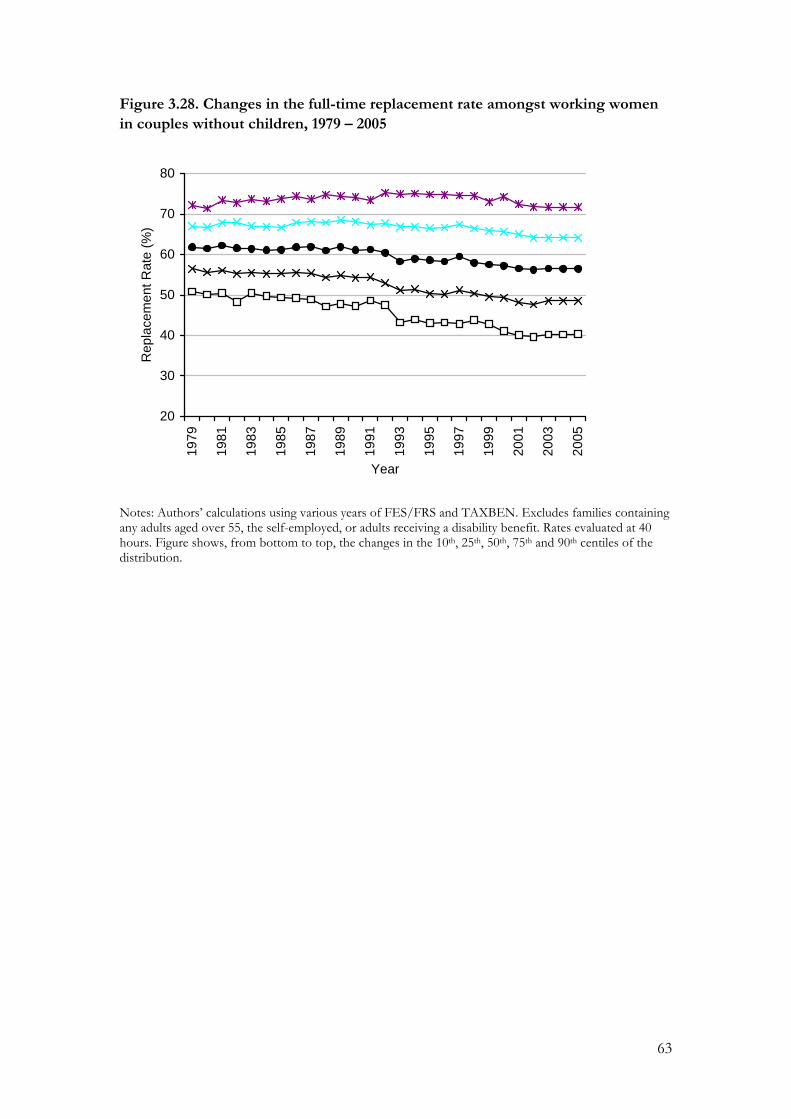
Figure 3.28. Changes in the full-time replacement rate amongst working women in couples without children, 1979 – 2005
20
30
40
50
60
70
8019
79
1981
1983
1985
1987
1989
1991
1993
1995
1997
1999
2001
2003
2005
Year
Rep
lace
men
t Rat
e (%
)
Notes: Authors’ calculations using various years of FES/FRS and TAXBEN. Excludes families containing any adults aged over 55, the self-employed, or adults receiving a disability benefit. Rates evaluated at 40 hours. Figure shows, from bottom to top, the changes in the 10th, 25th, 50th, 75th and 90th centiles of the distribution.
63
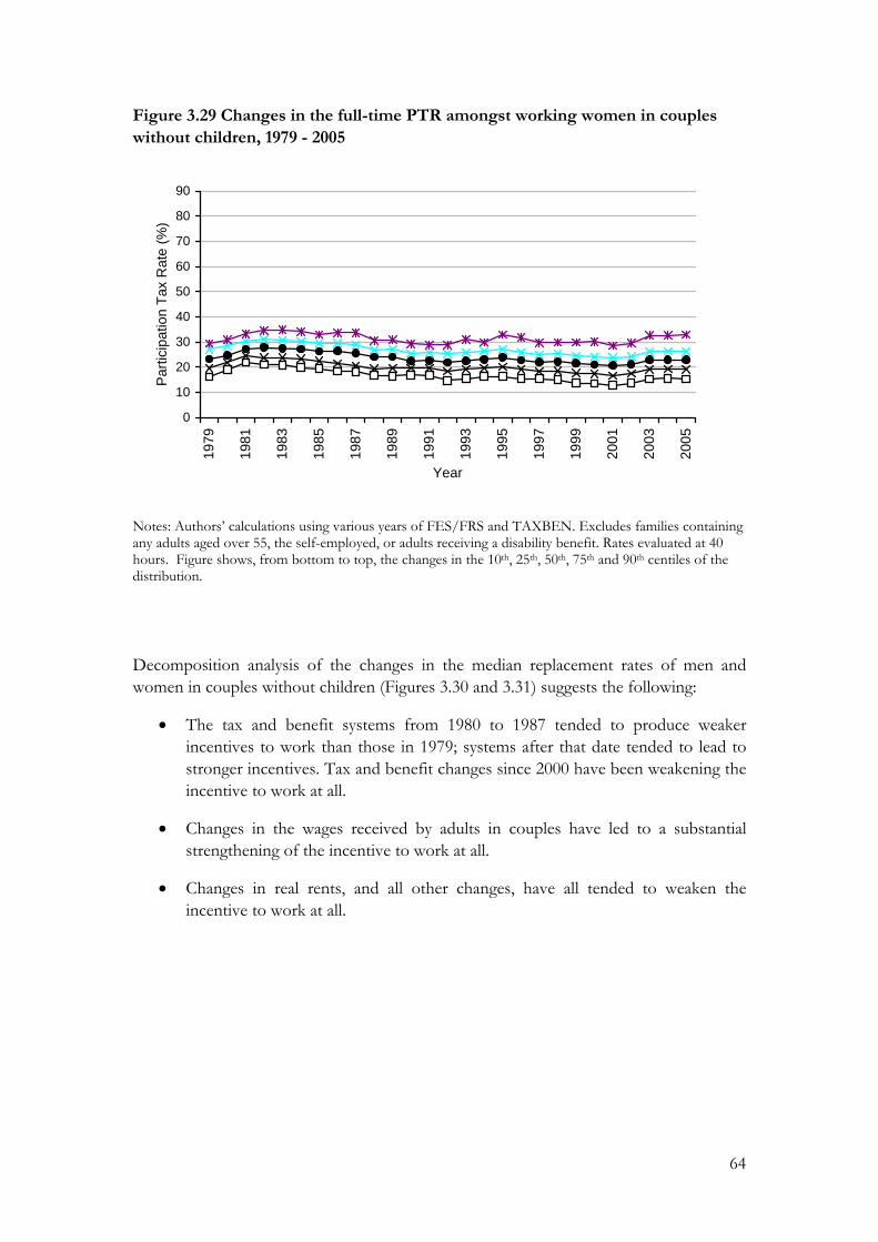
Figure 3.29 Changes in the full-time PTR amongst working women in couples without children, 1979 - 2005
0
10
20
30
40
50
60
70
80
9019
79
1981
1983
1985
1987
1989
1991
1993
1995
1997
1999
2001
2003
2005
Year
Par
ticip
atio
n Ta
x R
ate
(%)
Notes: Authors’ calculations using various years of FES/FRS and TAXBEN. Excludes families containing any adults aged over 55, the self-employed, or adults receiving a disability benefit. Rates evaluated at 40 hours. Figure shows, from bottom to top, the changes in the 10th, 25th, 50th, 75th and 90th centiles of the distribution.
Decomposition analysis of the changes in the median replacement rates of men and women in couples without children (Figures 3.30 and 3.31) suggests the following:
• The tax and benefit systems from 1980 to 1987 tended to produce weaker incentives to work than those in 1979; systems after that date tended to lead to stronger incentives. Tax and benefit changes since 2000 have been weakening the incentive to work at all.
• Changes in the wages received by adults in couples have led to a substantial strengthening of the incentive to work at all.
• Changes in real rents, and all other changes, have all tended to weaken the incentive to work at all.
64

Figure 3.30 Understanding changes in the median full-time replacement rate amongst working men in couples without children
-8
-6
-4
-2
0
2
4
1979
1981
1983
1985
1987
1989
1991
1993
1995
1997
1999
2001
2003
2005
Year
Rep
lace
men
t Rat
e (%
)
Tax Wages Rents Residual
Notes: Authors’ calculations using various years of FES/FRS and TAXBEN. Excludes families containing any adults aged over 55, the self-employed, or adults receiving a disability benefit. Rates evaluated at 40 hours. Figure 3.31 Understanding changes in the median full-time replacement rate amongst working women in couples without children
-8
-6
-4
-2
0
2
4
1979
1981
1983
1985
1987
1989
1991
1993
1995
1997
1999
2001
2003
2005
Year
Rep
lace
men
t Rat
e (%
)
Tax Wages Rents Residual
65
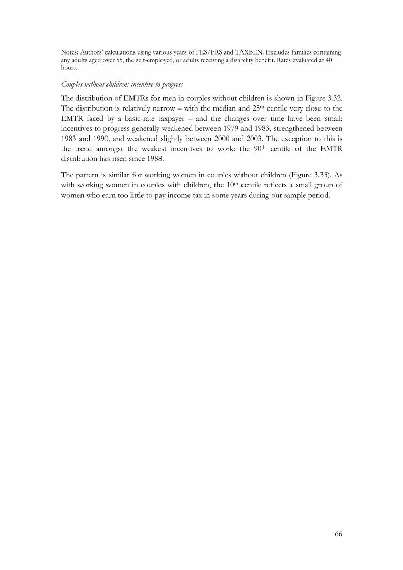
Notes: Authors’ calculations using various years of FES/FRS and TAXBEN. Excludes families containing any adults aged over 55, the self-employed, or adults receiving a disability benefit. Rates evaluated at 40 hours.
Couples without children: incentive to progress
The distribution of EMTRs for men in couples without children is shown in Figure 3.32. The distribution is relatively narrow – with the median and 25th centile very close to the EMTR faced by a basic-rate taxpayer – and the changes over time have been small: incentives to progress generally weakened between 1979 and 1983, strengthened between 1983 and 1990, and weakened slightly between 2000 and 2003. The exception to this is the trend amongst the weakest incentives to work: the 90th centile of the EMTR distribution has risen since 1988.
The pattern is similar for working women in couples without children (Figure 3.33). As with working women in couples with children, the 10th centile reflects a small group of women who earn too little to pay income tax in some years during our sample period.
66
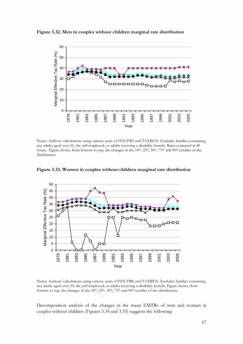
Figure 3.32. Men in couples without children marginal rate distribution
0
10
20
30
40
50
60
1979
1981
1983
1985
1987
1989
1991
1993
1995
1997
1999
2001
2003
2005
Year
Mar
gina
l Effe
ctiv
e Ta
x R
ate
(%)
Notes: Authors’ calculations using various years of FES/FRS and TAXBEN. Excludes families containing any adults aged over 55, the self-employed, or adults receiving a disability benefit. Rates evaluated at 40 hours. Figure shows, from bottom to top, the changes in the 10th, 25th, 50th, 75th and 90th centiles of the distribution.
Figure 3.33. Women in couples without children marginal rate distribution
0
5
10
15
20
25
30
35
40
45
50
1979
1981
1983
1985
1987
1989
1991
1993
1995
1997
1999
2001
2003
2005
Year
Mar
gina
l Effe
ctiv
e Ta
x R
ate
(%)
Notes: Authors’ calculations using various years of FES/FRS and TAXBEN. Excludes families containing any adults aged over 55, the self-employed, or adults receiving a disability benefit. Figure shows, from bottom to top, the changes in the 10th, 25th, 50th, 75th and 90th centiles of the distribution.
Decomposition analysis of the changes in the mean EMTRs of men and women in couples without children (Figures 3.34 and 3.35) suggests the following:
67

• The tax and benefit systems from 1980 to 1987 tended to produce weaker incentives to progress than those in 1979; systems after that date tended to lead to stronger incentives. Since 1999 (men) or 2002 (women), though, tax and benefit changes have been weakening incentives to progress.
• Changes in the wages received by adults in couples without children has led to a small weakening in incentives to progress compared to 1979.
• Changes in real rents have tended to weaken incentives to progress.
68
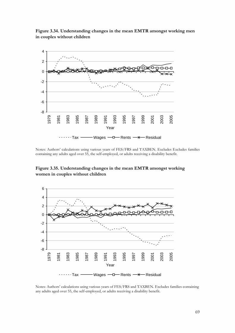
Figure 3.34. Understanding changes in the mean EMTR amongst working men in couples without children
-8
-6
-4
-2
0
2
419
79
1981
1983
1985
1987
1989
1991
1993
1995
1997
1999
2001
2003
2005
Year
Tax Wages Rents Residual
Notes: Authors’ calculations using various years of FES/FRS and TAXBEN. Excludes Excludes families containing any adults aged over 55, the self-employed, or adults receiving a disability benefit.
Figure 3.35. Understanding changes in the mean EMTR amongst working women in couples without children
-8
-6
-4
-2
0
2
4
6
1979
1981
1983
1985
1987
1989
1991
1993
1995
1997
1999
2001
2003
2005
Year
Tax Wages Rents Residual
Notes: Authors’ calculations using various years of FES/FRS and TAXBEN. Excludes families containing any adults aged over 55, the self-employed, or adults receiving a disability benefit.
69

Summary:
For both men and women in couples without children, the tax and benefit systems of the early and mid 1980s had weaker incentives (both incentives to work at all and incentives to progress) than those of the 1990s and 2000s. But the work incentives inherent in the tax and benefit system of 2005 are generally weaker than they were in 1999.
Growth in wages, particularly for women in couples without children, has also been very important in explaining the strengthening of the incentive to work at all.
3.3 Bringing it all together
What can we say about the main determinants of the changes in work incentives?
Considering the incentive to work at all:
• Growth in real wages over the period has tended to strengthen the incentive to work at all, as measured by the replacement rate.
• Over the 26 year period, real tax and benefit changes have strengthened incentives to work at all. The pattern has not been even, though. Generally, the tax and benefit systems in the early and mid 1980s led to weaker work incentives than that in 1979, those of the 1990s and 2000s led to stronger incentives: incentives crossed their 1979 level at some point between 1985 and 1989, depending on the measure. Real tax and benefit changes between 1979 and 1983 tended to weaken the incentive to work at all, those between 1983 and the late 1990s tended to strengthen it, but the most recent changes have tended to weaken it once more for most (not all) groups.
• Other changes in the economy, such as the growth in real rents acting through housing benefit, have tended to reduce the incentive to work at all.
The median incentive to progress is dominated by the large proportion of people whose EMTR is determined by the basic rate of income tax plus the national insurance contributions rate; changes in the median EMTR have been driven largely by real tax and benefit changes. For a more informative analysis, we decomposed changes in the mean, and found that:
• Changes in real wages since 1979 have had little net effect on average incentives to progress, only weakening them slightly. Increases in wages will tend to strengthen incentives to progress for adults who become too rich to quality for means-tested benefits or tax credits, or too rich to pay National Insurance contributions on their extra earnings, but weaken it for those who move onto higher income tax rates; our analysis suggests, therefore, that the last of these effects dominated, on average, over this whole period.
• Across the whole population, and over the 26 year period, real tax and benefit changes since 1979 have strengthened incentives to progress given current wage
70
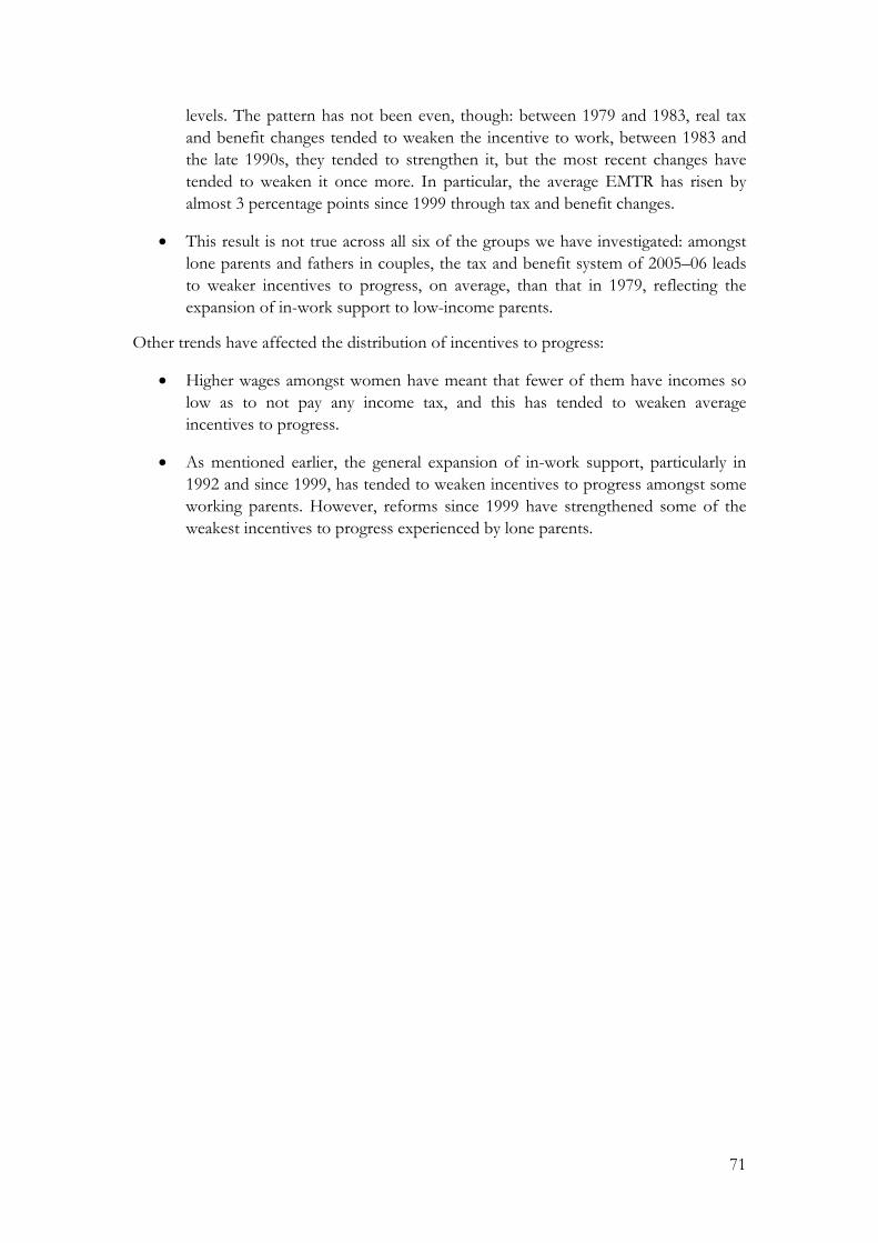
levels. The pattern has not been even, though: between 1979 and 1983, real tax and benefit changes tended to weaken the incentive to work, between 1983 and the late 1990s, they tended to strengthen it, but the most recent changes have tended to weaken it once more. In particular, the average EMTR has risen by almost 3 percentage points since 1999 through tax and benefit changes.
• This result is not true across all six of the groups we have investigated: amongst lone parents and fathers in couples, the tax and benefit system of 2005–06 leads to weaker incentives to progress, on average, than that in 1979, reflecting the expansion of in-work support to low-income parents.
Other trends have affected the distribution of incentives to progress:
• Higher wages amongst women have meant that fewer of them have incomes so low as to not pay any income tax, and this has tended to weaken average incentives to progress.
• As mentioned earlier, the general expansion of in-work support, particularly in 1992 and since 1999, has tended to weaken incentives to progress amongst some working parents. However, reforms since 1999 have strengthened some of the weakest incentives to progress experienced by lone parents.
71

References Adam, S. and Brewer, M. (2004), Supporting Families: The Financial Costs and Benefits of Children since 1975, Bristol: Policy Press.
Adam, S., Brewer, M. and Shephard, A. (2006), The Poverty Trade-Off: Work Incentives and Income Redistribution in Britain, Bristol: Policy Press.
Blundell, R. and MaCurdy, T. (1999), “Labour Supply: A Review of Alternative Approaches”, Chapter 27 of O. Ashenfelter and D. Card (eds.), Handbook of Labour Economics, vol. 3, pp.1559-1695, Amsterdam: North-Holland.
Brewer, M. and Browne, J. (2006), The Effect of the Working Families’ Tax Credit on Labour Market Participation, IFS Briefing Note no. 69, http://www.ifs.org.uk/bns/bn69.pdf.
Brewer, M and Shephard, A. (2004) Has Labour Made Work Pay?, http://www.jrf.org.uk/bookshop/eBooks/1859352626.pdf.
Brewer, M and Shephard, A. (2005), Employment and the Labour Market, IFS 2005 Election Briefing Note no. 5, http://www.ifs.org.uk/bns/05ebn5.pdf.
Brewer, M., Clark, T. and Goodman, A. (2003), ‘What really happened to child poverty in the UK under Labour’s first term?’, Economic Journal, vol. 113, pp. F240–57.
Brewer, M., Duncan, A., Shephard, A. Suárez, M. (2005a) “Did Working Families' Tax Credit work? The final evaluation of the impact of in-work support on parents' labour supply and take-up behaviour in the UK”, Inland Revenue Working Paper 2, http://www.hmrc.gov.uk/research/ifs-laboursupply.pdf.
Brewer, M., Goodman, A., Shaw, J. and Shephard, A. (2005b), Poverty and Inequality in Britain: 2005, Commentary no. 99, London: Institute for Fiscal Studies
Brewer, M., Goodman, A., Shaw, J. and Sibieta, L. (2006), Poverty and Inequality in Britain: 2006, Commentary no. 101, London: Institute for Fiscal Studies
Clark, T. and Leicester, A. (2004), “Inequality and two decades of British tax and benefit reform”, Fiscal Studies, Vol. 25, No. 2, pp. 129-158.
Dickens, R. & Ellwood, D. (2003). “Child Poverty in Britain and the United States,” Economic Journal, vol. 113(488), F219-F239.
Evans, M. and Eyre, J. (2004). The Opportunities of a Lifetime, Bristol: The Policy Press.
Gentry, W. M. & Hubbard, R. G. (2004). "The effects of progressive income taxation on job turnover," Journal of Public Economics, vol. 88(11), pages 2301-2322.
Giles, C., Johnson, P. and McCrae, J. (1997) “Housing benefit and financial returns to employment for tenants in the social sector”, Fiscal Studies, Vol. 18, No. 1.
Gregg, P., Johnson, P. and Reed, H., (1999) Entering work and the British tax and benefit system, London: IFS.
72

Heckman, J. (1974), “Shadow Prices, Market Wages and Labour Supply”, Econometrica, 46, 695-712.
Heckman, J. (1979), “Sample Selection Bias as a Specification Error.” Econometrica, 47(1): 153-161.
Sutherland, H. (1997), “Women, Men and the Redistribution of Income”, Fiscal Studies, 18 (1), 1-22.
Sutherland, H., Sefton, T. and Piachaud, D. (2003), Poverty in Britain, York: Joseph Rowntree Foundation.
73