t I

9 : ,J *

FINAL REPORT - PHASE I A CAVITY RADIOMETER FOR EARTH ALBEDO MEASUREMENT

SBsIR PROPOSAL NUMBER 86.1-08.02-1035

October 18, 1987

This work was supported by: National Aeronautics and Space Asministration

Goddard Space Flight Center Under Contract NAS5- 30059

I

L

(NASA-CR-lE1385) A CAVITY BADIONETEB P 3 k N 87- 2980 5 EARTH ALBEDO HEASUREHENT, PHASE 1 F i n a l Report (Technica l Measurements) 34 p A v a i l : NTIS HC A03/MF A01 CSCL. lit8 Unclas

GJ/35 0102708

TECHNICAL MEASUREMENTS, INC. La Canada, California

https://ntrs.nasa.gov/search.jsp?R=19870020372 2020-03-16T01:31:17+00:00Z

SBIR pROR3SA.L JWMBER 86.1-08.02-1035

Radiometric measurements of the directional albedo of the Earth requires a detector with a flat response from 0.2 to 50 microns, a response time of about tho seconds, a sensitivity of the order of 0.02 mw/cm , and a measurement uncertainty of less than 5%. Absolute cavity radianeters easily meet the spectral response and accuracy requirements for Earth albedo measurements, but the radiometers available today lack the necessary sensitivity and response time.

2

In this effort, the specific innovations addressed were the developnent of a very low thermal mass cavity and printed/deposited thermocouple sensing elements which were incorporated into the radiometer design to produce a sensitive, fast response, absolute radiometer. The new cavity is applicable to the measurement of the reflected and radiated fluxes fromthe earth's surface and lower atmosphere from low earth orbit satellites. The effort consisted of requirements ard thermal analysis: design, construction, and test of prototype elements of the black cavity and sensor elements to show proof-of-concept.

The results obtained indicate that a black body cavity sensor that has inherently a flat response from 0.2 to 50 microns can be produced which has a sensitivity of at least 0.02 mw/cm per micro volt output and with a time constant of less than tho seconds. Additional work is required to develop the required thermopile.

2

~ I C A L M E A S U R F M E N I ' S , INC La Canada, California

.. .--- I '.

c

PAGE

PRIXTECT ~Y........................................................l P m J E r OBJECrIvE

I. General ............................................... 1 11. Sensor Requirements ..................................... 2

111. Optimum Cavity Sensor ................................... 3

I. Requirements Analysis ................................... 3 11. Thermal Analysis ........................................ 6 111. Cavity Desi gn..........................................17 IV. Thermopile Desi gn...................................... 19 V. Manufacturing Processes

A. Electrofomi ng. . . . . . . . . . . . . . . . . . . . . . . . . . . . . . . . . . 21 B. Thermopiles ..................................... 25

VI. Test Item Manufacture .................................. 26 V I I . Test Pr~ram...........................................26

WORKED PERFOEZMED

RESULTS CBTAINED I. Analysis and Mamufacturing Fksults.....................28 11. Test ~sults.. ......................................... 29 111. Performance Estimates .................................. 30

ESTIMATE QF "NI(IAL E'EASIBILI TY..................................... 30 CONTNCT REpOFtTING mwI REMENIS....................................... 31 STATEMEW W I F y I N G LEVEL OF EFEOKT'..................................31 FIGURES

1 2 3 4

Developnent of 'Two Cone Geunetry.. ..................... .8

(Xlter Cone Dimensionless Time Constant.................13 Mid-mint Receptor Geanet ry............................ 16 High Sensitivity Fast Time Constant Radiometer.........18

Radiometric measurements of the directional albedo of the Earth requires a detector with a flat response from 0.2 to 50 microns, a response time of about t w seconds, a sensitivity of the order of 0.02 mw/cm , and a measurement uncertainty of less than 5%. Absolute cavity radiometers easily meet the spectral response and accuracy requirements for Earth albedo measurements, but the radiometers available today lack the necessary sensitivity and response time.

2

In this effort, the specific innovations addressed were the developnent of a very low thermal mass cavity and printed/deposited thermocouple sensing elements which were incorporated into the radiometer design to produce a sensitive, fast response, absolute radiometer. ?he new cavity is applicable to the measurement of the reflected and radiated fluxes fromthe earth's surface and lower atmosphere from low earth orbit satellites. The effort consisted of requirements and thermal analysis; design, construction, and test of prototype elements of the black cavity and sensor elements to show proof-of-concept .

m e results cbtained s h o w that with further developent, a black body cavity sensor can be produced which meets all of the critical requirements for a top-of-the-atmosphere earth radiation W g e t instrument,

I. General

The end objective of the multiphased SBIR effort is the development of an Absolute Cavity Array Instrument (ACAI) suitable for measuring the top of the atmosphere flux from the full earth disk visible from an orbiting satellite at approximately 830km altitude. The ACAI would be composed of an number of detectors mounted in an array to measure the radiation field below the satellite. By using an array of fixed sensors of the absolute cavity type,

P A a 1

". *

problems associated with mechanical motion and spectral response are eliminated. The advantages to be derived fran the use of the absolute cavity sensors should be the following:

1.

2.

3.

4.

The current feasiblity

Measurements needirq M spectral corrections. Self-calibrating, direct energy measurements, with high stability. Measurements directly comparable to ERB measurements. A mechanically simple device, without moving mirrors.

phase of the research is centered on the cavity sensor: the of providing an absolute cavity sensor with the required

sensitivity and response time to make the required measurements. The next phase of the research will address the integratim of the sensor cavity into an instrument capable of making the desired measurements of earth lS3A albedo. And then, the research will address issues associated with inflight calibration, field-of-view and spatial convolution, and overall instrument measurement accuracy and stability.

11. Sensor Requirements

For the ACAI to have the desired sensitivity, the cavity sensor must provide an electrical signal greater than 1 microvolt for the unit of energy corresponding to the required resolution. This equates to a sensitivity of at least 0.02 mw/cm /pv. The standard Kendall cavity used in the Mk VI radiometer has a sensitivity of m l y .06 mw/cm /pv. Therefore an improvement of over three is required ard a tarqet.improvement of 10 is desired.

2

2

The stated requirement for response time (l/e) is less than t m seconds. The standard Kendall cavity exhibits a response time of approximately 6 seconds. Again, an improvement of at least three is required. ?his requirement is the most difficult to meet.

The spectral sensitivity of the cavity is required to be flat from .25 to 50

microns. The inside surface of ?MI cavities are coated with 3Mblack velvet. This mating is m t specular, and has a certain amount of retro-reflectance.

PAGE 2

1 Y

,

Measurements of emittance of this type cavity were made by NBS on a Mk VI

cavity using a laser for irradiance and a conical pyrolytic receptor to measure the emittance. The results of this test gave an overall reflectance of 0.0021. A correction factor is amlied to account for this loss of radiant prower. No direct measurements of spectral sensitivity have been made, but it is quite certain that the spectral response is flat over the solar spectrum. The radiometer has been tested by the radiance from a black body warmed to a temperature of loo C above the temperature of the radiometer (at 30°). The radiometer gives a very strong response, indicating spectral sensitivity at long wavelengths.

This corresponds with analytic studies performed by JPL and ?MI.

111. Optimum Cavity Sensor

The optimum cavity design for the ACAI represents a trade of size, sensitivity, and time response. It is beyond the scope of this effort to optimize a cavity design for -1, but it is within scope to determine the controlling parameters, to verify them, ard to demnstrate the feasiblity of achieving a satisfactory Sensor. 'Ihe reason that an optimum design can not be obtained at this stage is that the performance of the sensor is heavily dependent on the design of the view limiter and of the containing body. These, in turn, are driven by considerations of weight, size, and experiment design. In this effort we intend to show that we have sufficient control of the important variables and that instruments which can meet ACAI requirements can be produced.

I. Requirements Analysis

The scope of the requirements analysis is to establish an acceptable approach to the evaluation of the effect of instrument time constant on the interpretation of the data obtained frm an open aperture cavity radiometer swept across a variable scene. ?his, in a reverse application, can provide the specification of time constant (together with other instrument parameters)

req[uired for the interpretation of gathered experimental data with respect to the achievement of stated scientific objectives.

In a "shuttered" application where the "scene" goes from one fixed, constant value to a second fixed value, the conventional time constant is a direct measure of the reqyired settling time to reach the second value within a given error of the measurement. For a continuously changing scene or a swept scene, a meaningful measure of the time-related accuracy is different and we suggest consideration of the steady state error in following a step change in the scene during the time the step propagates through the scene. This concept will now be developed.

A one dimensional &el is assumed. For given values of radiometer aperture width, view limiter width, distance to view limiter and finally operating altitude, tm scene ar object sizes are determined. The first and smaller, width sl, is that region hich is seen by the entire measurement aperture of the instrument. ?he second, total width s2 to outer edges, are the additional regions an both sides of the first; these do not fill the measurement aperture because they are cut off in various amounts by the view limiter. Now define tl and t2 as s /v and s2/v where v is the (orbital) velocity of the sweeping motion.

1

Next consider the effect of the step change in radiated power as it propagates through the instrument view due to orbital motion. The step is perpendicular to the direction of motion. As the instrument is swept across this location, the region s1 provides a ramp inplt of time length tl. The instrument also sees a pre-ramp and a post-ramp with a smaller slope; the duration is t2, which is symetrically spaced around ti. The actual response of the instrument will be between that of the response to a single, unit amplitude, ramp of duration tl, and to a single, unit amplitude, ramp of duration t2 greater than

5' The response of a single time constant device (time constant = to) to a ramp

inpt of unspecified duration of the shape ar magnitude Wo t/tl is:

It is readily seen that W(0) = 0, as it must be. Here t = 0 is the time when the ramp starts, i .e. when the edge of the ramp canes into view. For large t , t larger than to, the instrument output eventually follows the ramp inpt with a simple time delay equal to to, the instrument time oonstant.

For the above to be applicable to the experimental conditions here where the ramp times (tl or t ) are finite, the value of to must be significantly smaller than the ramp time: the value of to must be at least less than 0.2 tl and preferably less than 0.1 tl . (For the case of t larger than tl the instrument is so slow that it can not tell the difference between a ramp input and a "shuttered" step inFt.)

2

0

"Is, for the case here of following with time delay to, the error, w, in following the actual power input to the instrument (which is all it can be expected to measure) from a step change of power, W, at the scene is given

by: w / w = t o / tl

This error exists during the center portion of the ramp. The transient departure at the start and the transient closure at the end of the ramp are of the form {1 - exp(-t/to)]. For t2 = m tl, the error may be considered boLlnded: not as much as to/tl but not less than to/t2 = to / m tl . We now advocate the incorporation of the above description of instrument time related error to a step d m q e at the scene into the combined tasks of the specification and design of, 1) the instrument to make the measurement, 2) the conditions under which the experiment is to be carried out, and 3 ) the interpretation of the acquired data. '

A point on the curve is now given. from an altitude of 830 km where the orbital velocity is about 7.4 km/sec:

With a scene spot size of 250 km viewed

tl = 250/7.4 = 33.8 sec

For a step change of 1/2 full scale in the scene (clouds. no clouds during sunlight) and an instrument time constant of 3 . 3 8 sec the error in not following the step is:

.38/3 ,8) = /2O = 5% of full scale

The above analysis has focused entirely on the effect of instrument time constant. It must be remembered that the time constant "tracking" error, just discussed, does not relate or cause an error of the intregal of the energy of the step change of radiation, but cmly an additional smearing of the step: the finite width of the aperture with its view limiter wings causes the first smear. Mditionally, the m u n t of motion smear and instantanems measurement error can be estimated from the rate-of-change in the recorded data for a clean, abrupt, single step change. 'Ihe absolute sensitivity and resolution of the instrument is certainly of great importance; the physical reality is that these latter are related directly to the size of the instrument whereas the time constant increases (undesirably so) as the square of the linear size. The intent of this requirements analysis is to provide a useable measure of the effect of time constant for combination with other instrument and experiment requirements.

11. Thermal Analysis

A major effort was made to produce a theoretical, mathematically rigorous description of the transient thermal flow through simplified gemetries that could adequately represent actual cavity and thermal resistor configurations. It was intended that this be used in meaningful evaluations of the model cavities to be produced using thin wall electroforming techniques.

The basic coordinate system for the constant wall thickness, conical receptor is cylindrical: r, theta and z. (Cut out a pie shaped portion of a thin flat pancake and form the balance into a cone.) The only spatial variable is the radial distance r; flow is along lines of constant theta, and the walls are sufficiently thin, z direction, that is assumed there is negligible temperature difference and flow in that direction. The flow along the r direction, of course, is not spatially uniform; it diverges or converges with radial distance.

Tb start, the basic single flow parameter equations for the three systems were

P A a 6

- set down: linear (Cartesian), cylindrical, and spherical

T 1

thickness along cavity walls). The form of the basic time constant was determined for each system (referenced later in this report). Most of this effort was the gathering together of classical mathematical solutions available in m y places: the Wrpose was to assemble the tools that could be useful in analysis of actual cavity a d receptor configurations.

During this time, the concept emerged of a simple cone receptor with a mid-point thermal resistor as the minimum time constant configuration. One of the major driving forces was the fact that it was felt that this geometry could be quite rigorously analyzed. The measured performance should compare well with the prediction for thermal time constant. The balance of the thermal analysis performed here is based on this configuration, using the Bessel function solutions to the cylindrical coordinate configuration.

The mid-point thermal resistor configuration is built up from two conical pieces. The outer portion of the inner mne, which contains the closed apex, is folded over and down to form (a part of) the thermal resistor. ?he outer cone has a hole as its inner edge, and its lower portion is slit and split outward to form (the balance of) the thermal resistor. In the combined parts of the resistor the excess material from the inner cone fills the vacant spaces between the slits in the outer cone: the result is a cylindrical thermal resistor of constant thickness equal to twice that the of conical, receptor, prticn. The rigorous transient thermal analysis model consists of starting at time zero with a representative

The details are given in Figure 1.

temperature profile along the conical sections. This profile tapers to a constant reference temperature at the lower edge of the thermal resistor; the local temperature is measured as a temperature difference from this reference. At time equals zero the heat flux producing the initial temperature profile is considered to be removed and the temperature falls to the constant reference temperature at a rate indicative of the thermal time constant.

The mathematical form for the cylindrical case is well known and the general solution is given by:

PAGE 7

,

PAGE 8

T 1

dhere : a 2= k/cp = corductivity/volume heat capacity = Bessel functions of zero order yo

p s = series of inverse lengths required to satisfy the reference termperature condition

= series of temperatures magnitudes that satisfy the initial temperature distribution:

When applied to the inner cone with a total length ro including the thermal resistor portion and mntaining the center apex at r = 0, first all Bs must be zero since Y ( 0 ) is infinite. Next since, T(ro,t) = 0 it is required that

' where jo are the zeros of Jo. Defining 0

I S Jo(g sro) = 0 and thus (psro) = J O I S

= I/& 2ps2 the quation for T becomes: tS

T(r,t) = Z A e-t'ts J ( j r/ro) S 0 0,s

where ts = ro / ( j O I s l2 = time constants of the components.

For the several components of the solution a short table of relative time constants demonstrates the concept of the dominant time constant which will be used subsequently:

S '0,s ts/tl 1 2.4048 1.000 2 5.5201 .190 3 8.6537 .077 4 11.7915 .0415

Thus it is seen that the canponent terms for s = 2,3,4, etc. decay much more rapidly than for s = 1 and the tl time constant will dominate the transient behavior for the temperature profiles to be encountered in real cavities. This is discussed further shortly.

It will be illustrative to consider briefly other coordinant systems, Cartesian (linear) and spherical. The linear case represents a t m dimensional trough shaped cavity and the spherical the case of cavity thickness zero at center apex and increasing linearly with distance outward.

PA= 9

For the linear case with a length of xo to the center of the cavity:

The n here clearly represents a series of harmonics, and for dT/dx = zero at x = xo at

For the

the center of the "trough", n must be odd. The time constants are:

2 tn = (x0 / a 2, / (n17'/2)

spherical geometry case the solutions are of the form:

sin(n ~~'x/xo)/(x/xo).

The zeros are at IIX = f l a n d the resulting time constants are:

A tabular comparison of the dominant time constants shows the effect of geometry.

Geametry Linear Cy1 indr ical spherical Math form Trig Bessel (Sin x)/x Daninant time constant ( 2 / c l 2 (1/jo,1)2 (l/m

= 4/n2 = 1. 708/H2 = 1/n2

For the cylindrical case the daninant time constant is less than half that of the trough and for the spherical case it would be only one fourth. The spherical case, with its tapered walls, was not considered for implementation at this time.

The linear geometry case can be used time constant is indeed dominant for distributions. The initial temperature

to show quite easily that the daninant representative initial temperature distribution is given w:

, n odd cnly

PA= 10

i

By ao&ining small amounts of 3rd, 5th, etc. harmonics, the temperature rise can be made quite linear from x = 0 to some fraction of xo, e.g 1/3 . This corresponds to the thermal resistor portion where the constant heat flux produces a linear temperature drop. Beyond this "resistor" region the temperature profile continues to rise to a maximum at xo, the center of the trough. This is precisely the case for same form of sensibly constant heat flux absorbtion in this, the receptor, portions of the device. The relative time constants decrease as 1/9, 1/25. 1/49, etc. of the dominant time constant. 73-11.1s even if there are significant quantities of the harmonics (relative to the n=l fundamental), these will die out rapidly. The ultimately dominant transient temperature distribution will be the quarter period sinusoid that will decay at the dominant, n=1, time constant rate. The Bessel functions are basically trigonometric functions whose amplitude falls off with distance (approach sin x / x for large x); the spherical case behaves as sin x/x. The concept of harmonics and the behavior of these harmonics is directly transferable frm the linear, simple trigonometric, case to these.

The basic analytical work presented in the several previous paragraphs for the inner cone can be found in many text books. The concept of the daminant time constant and the representative initial temperature distributions has been specifically tailored to the circumstances of cavity receptors. The analysis to follow for the outer cone prtion is considered to be new work, original to the specific requirements here.

For the outer cone, the task is to determine the dominant time constant for a two parameter system defined by an inner dge radial distance rl and an outer edge radial'distance, r2 instead of the single parameter r for the inner cone. ?he boundary mndition at rl is constant (reference) temperature since this edge will ultimately be the bottom of the thermal resistor. At r2, the outer edge of this outer cone, the requirement is that dT/dr = 0; no heat is conducted along the aone at this pint since this is an dge that is thermally insulated. ?he Yo Bessel solution is now acceptable since r is always larger than zero. The single solutian for the dminant time constant will be sought rather than the general sum of all the possible "harmonics". The general solution for the outer cone is:

0

PAGE: 11

i

T 1

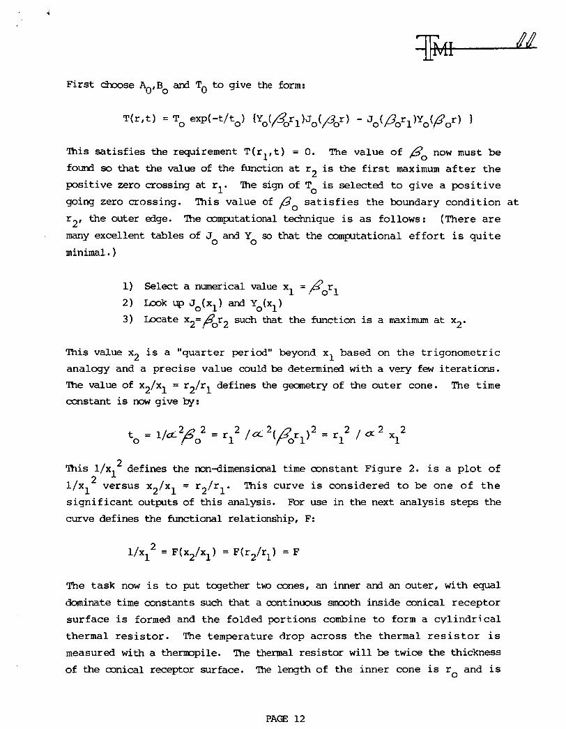
First choose A B and To to give the form: 0' 0

This satisfies the requirement T(rl,t) = 0. The value of Bo now must be feud so that the value of the function at r2 is the first maximum after the positive zero crossing at rl. ?he sign of T is selected to give a positive going zero crossing. r the outer dge. ?he computational technique is as follows: (There are many excellent tables of J and Yo so that the comptational effort is quite minimal. )

0 This value of Po satisfies the boundary condition at

2' 0

1) Select a numerical value x1 =,Forl 2) m k UP Jo(xl) and Yo(xl)

Locate x2= p0r2 such that the function is a maximum at x2. 3)

This value x2 is a "quarter period" beyond x1 based on the trigonometric analogy and a precise value could be determined with a very few iterations. The value of x2/x1 = r2/r1 defines the geometry of the outer cone. The time constant is now give by:

2 = 1/d2~: = r12 /CL 2(porl)2 = r 1 2 / a ' x 1

This 1/x12 defines the non-dimensional time constant Figure 2. is a plot of 1/x12 versus x2/x1 = r2/rl. This curve is considered to be one of the significant outputs of this analysis. For use in the next analysis steps the curve defines the functional relationship, F:

1/x12 = F(x2/x1) = F(r 2 1 /r ) = F

The task now is to put together tm cones, an inner and an outer, with equal dominate time constants such that a continuous smooth inside conical receptor surface is formed and the folded portions combine to form a cylindrical thermal resistor. The temperature drop across the thermal resistor is measured with a thermopile. The thermal resistor will be twice the thickness of the aonical receptor surface. The length of the inner cone is ro and is

PAGE 12

t: e

s i

TOP OF SCALE VALUE FOR F = 1/x12 = ORDINATE

0.1 1.0

I r ’

OUTER CONE DIMENSIONLESS TIME CONSTANT

FIGURE -2

PAGE 13

c

the basic reference dimension. A length k xo of this axe is folded over to produce a thermal resistor of length k x This requires that rl=(l- 2 k)ro so that when an equal length, k ro, of the outer cone is folded out to complete the thermal resistor, the tho cones match to form a smooth receptor surface. The inner and outer time constants which are set equal are given

0'

w:

= r /a 2 ( jo,1)2 = 0.1729 r: /cZ: 2 tin o

2 2 2 2 2 tout =rl /tc: x1 = F r l /c;C

F = 0.1729 (ro/rl)2 = 0.1729 / (1- 2 k )2

The combined cone has m w been defined by two parameters, ro and k. Small values of k W i l l give large values of r2, the "aperture size" of the cone, with resulting large energy input but short length thermal resistors with small temperature drops for measurement by the thermopile. Smaller values of k decrease the aperture area and energy received but increase the thermal resistor length and the output voltage. In the next paragraphs the maximum (relative) sensitivity is found.

In high absolute cavity radiometers, a deep cavity is used. This provides a high cavity enhancement factor the reduces the effect of lack of precise knowledge of the emissivity of the receptor surface. -ever, the larger size and longer heat flow paths greatly increase the time constant. For here a simple conical shape is proposed with half cone angles of 30 degrees to provide is based for the resistor

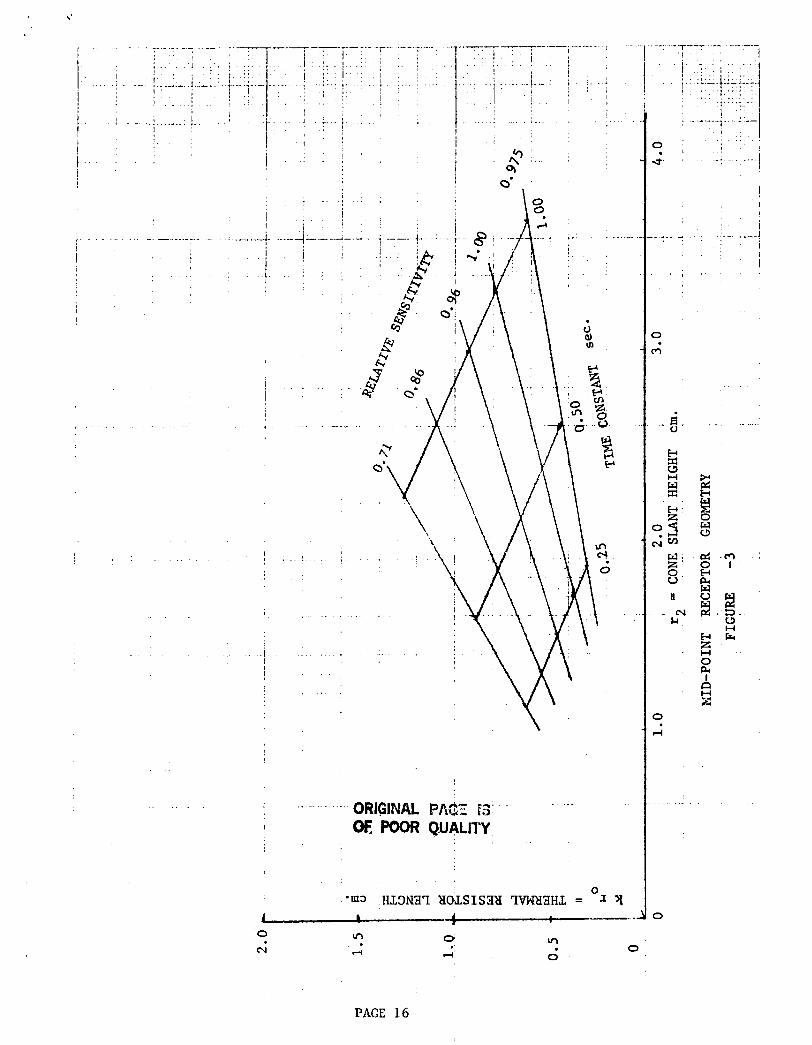
at least some cavity enhancement. The following sensitivity analysis cn a constant cone angle ard hence produces a relative sensitivity constant half angle, phi, as a function of the length of the thermal and the time constant. At a given flux density input:

bwer = p0 (r2 sin+)2 = p0 sin 2 9 (r2/r012 ro 2

Circumference of thermal resistor = 2 (1 - k)ro sin p Length of thermal resistor = k ro Temperature drop across thermal resistor is proportional to: (Power) (Length) /(Circumference)

Number of themuples is proportional to the circumference.

P A a 14

Voltage produced is thus proportional to: (Temp drop) (Circumference) = (Pbwer) (Length)

n n n L L L = sin r2/ro) ro (k ro) = sin2? rO3 [ k (r2/ro)2 1

Thus at constant half cone angle and at a given time constant (which determines the value of ro) the maximum electrical output is at the maximum of the product k ( r2/ro)' . This product maximizes at k=O. 252. Silver is now selected as the cone and resistor material with its low value of cz. :

1/a2 = 0.580

The graph of Figure 3 constants of 0.25, 0.50

2 sec / an

is now produced from these relationships for time and 1.0 seconds. For half cone angles of 30° The

slant length of the cone is also equal to the diameter at the outer edge. A

long thermal resistor is desired for several reasons, e.g. attachment of the required electrical insulation barrier to isolate the thermopile junctions and attachment of the thermopile itself. ?he graph shows that the resistor length can be sensibly increased (also a smaller aperature and thus smaller instrument size itself is cbtained) with only a modest and probably a very acceptable decrease in relative sensitivity. This curve is considered to be the second significant output of this analysis.

In summary, the basic objective of this transient thermal analysis was to provide tools and guidance for the selection of the size and geometry of the ultra light receptor cones and associated mid-point thermal resistors. Both the magnitude of the time constant and the geometric features for minimizing this magnitude were obtained. The term "mid-point" is a misnomer; in actual practice the location of the resistor is well toward the outer edge of the cone; thermal flux flaw along the diverging inner portion is less impeded than the converging flow from the outer portion. mestions and concerns about the proper matching of the initial temperature conditions in the combining of the t w folded prts to make the thermal resister are valid. Wwever, it is felt that the dominant time constant concept is a valid approach for the purpose here; "higher harmonic" terms do exist in an actual initial temperature distribution caused by the actual input thermal flux. But these will decay rapidly. This dominant time constant concept is intrinsic to this analysis

PAGE 15

\'

I

i ! i i i i j I

!

I

I I

i

. . . .

! . . . .

, .

. . . .

. ~ __ .._- . , I : ' ; . . . . ' I . . ; . . . .

I I . I I . i : : . . . . . . . .

1.: _._... ! ' ' p; : . . . j . . . . . ! .

I .

..

....... I

:. . 2

I I

.....

i

~ - . . . .

.. ! . . . ; . - : I . . . . . I : ! I. . :

. . . . . . . 3 . .

...

I

. . .

I

\o, . - . I . ,

I I

c . . . . - . - . .

. . . . . i . .

! .~ . . . . . . . .

I . . . . . . . . Cki .m . : 0 1

. . . . . . . . ~.

w

I . . . . . .

. . . . . . . . .i I

. .

\ . .

0

hl C

PAGE 16

and is mnsidered a third significant analysis output.

111. Cavity Design

Wification of a standard black cavity sensor both by changes in geometry and by new technological advances in fabrication methods were explored. Two

cavity designs were considered: the standard TMI design modified only for manufacturing by new methods, and a new cone cavity design attempting to achieve maximum performance with sensitivity greatly increased and time constant significantly decreased. Changing cavity shape is a trade of response time for cavity absorptivity, and uncertainty of measurement in long term use. The standard Kendall cavity design has an enhansement of a factor of six over a flat plate and a factor of 2 over a 30° cone. An additional factor that can be considered is giving up the self-calibratim feature to gain response time.

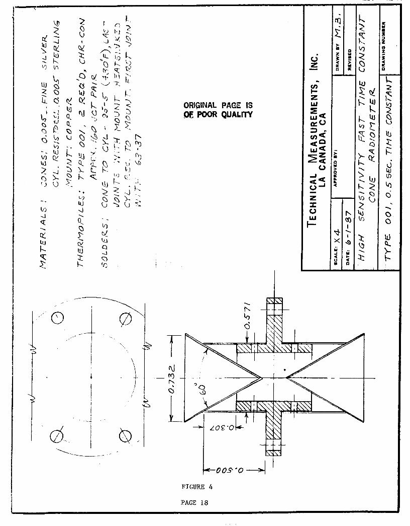
A study of cavity geometry considering parameters of aperture area, wall thickness, (thermal mass) of the flux receptor versus the thermal resistance and diffusivity of metals as well as the geometry of the thermal resistor was made. The geometry of the combinatian of thermal resistor and flux receptor was also considered with respect to optimization of time constant and transient effects. The resulting design was a cavity sensor configuration consisting of t m symmetrical cone-thermal resistor sensors mounted back to back on a heat sink temperature disc (See Figure 4) . The functian of this disc is to provide a reference temperature to hich the temperature gradient caused by incoming irradiance can be measured. The opposite or back looking sensor is covered so that it sees no incoming irradiance but is used to compensate for any heat flux which may be entering or leaving the common mounting disc. ?he electrical signal from the "compensating" cavity sensor is connected so as to oppose the signal fran the measuriq cavity. If the t m back-to-back cavity sensors are perfectly physically matched any signals caused in the two sensors by heat flux entering or leaving the heat sink mounting disk will be cancelled and m t show up in the measurement.

The manufacture of perfectly symmetrical cavity and thermal resistor sensors is made feasible by using the electroforming process for fabrication. This

PAGE 17

4

.

’.

\

I I

_ -

ORIGINAL PAGE IS .DE POOR QUALITY

PAGE 18

process assures the precise physical matching of cavities by the use of a common mandrel on which to form the components and by using the integral of time and current to provide an exact knowledge of the mass of silver deposited on the mandrel. A discussion of the electroformiq process will be given later in this report.

Other fabrication techniques also help maintain the necessary thermal symmetry. Q?e of these consists of the careful use of silver and tin solder for joining components. In this process care is taken to use consistent solder weights and to minimize tinning of the silver on areas other than in the joints. Care is taken to "wet" these joints thoroughly and to eliminate joint gap spaces in order to provide the greatest possible heat transfer across joints.

Another design feature kith aids in assuring thermal symmetry is the use of identical "postage stamp'' type printed circuit thermopiles. An identical thermopile strip is wrapped around the thermal resistor of each opposinq sensor to measure the temperature drop between the isothermal ring formed at the junction between the receptor cone and the thermal resistor cylinder and the heat sink temperature. Since all thermopiles are phVsically identical their effect an thermal resistor values are equal and symmetry is maintained.

IV Thermopile Design

The objectives of thempile design were to obtain the greatest output voltage with minimum effect on time constant. Since the radiometer design incorporated a geometry symmetrical about the mounting disc it was also decided to use an identical thermopile on each side and to connect the thermopiles electrically in series oppostion. This design differs frm the present design kith places the measuring junctions about the isothermal ring of the measuring cavity and the reference junctions about the isothermal ring of the compensating cavity. The new design doubles the actual number of junctions used but permits a wrap around applicatim of a thermopiles "postage stamp" strip rather than having to route the between junction wiring through holes in the reference temperature munting disc. This type of mounting of the thermopiles greatly simplified fabrication of the cavity assembly as well as enhancing the performance.

PAGE 19

,

I T 1

A local strain gage-thermocouple manufacturer, Micro Engineering, Inc. was selected to help develop the printed circuit thermopile. Since this development was considered to be the most difficult task of the project and since we had knowledge of the capbility of this company we decided to work with them on this developnent. We suhnitted our desired specifications viz, maximum output, maximum number of junctions, thinnest backing material and minimal electrical resistance. We also provided drawings showing the desired geometry, connection means and possible junction form.

Micro Engineering came up with an alternative geometry and junction fabrication method which exceeded our expectations. The design utilized a wrap around strip which in the case of our short time constant sensor design would provide 176 pair of junctions per strip. This design, provided by Micro mineering is considered proprietary by them.

Attempts were made to fabricate the thermopiles on 0.3 mil Kapton as a minimum thickness backing material. Both using multiple thermopiles per backing plate as well as using only a single thermopile proved too difficult to fabricate. A change to 1.0 mil backing material provdd the manufacturing method to be possible but will results in poorer transient heat transfer to the junctions. A compromise using 0.5 mil Kanton backing appears feasible for the design presently being used. The electrical resistance of a thermopile of 176 junction pair is presently in the order of four thousarrd ohms which is still compatible with presently available amplifier input impedance requirements.

PA- 20

T 1 -

Three Severe problems were encountered: weak bonding of the thermocouple material to the Kapton, the second thermocouple material would not release from the Teflon backing when transfered to the kipton to form the thermopile junction, and the registratim of the t m parts of the thermocouple pattern. Each of these problems have been solved in other apylications and are solvable for fabrication of the desired thermopile with additional time. However, because of the time constraint of this contract effort, wrk was stopped when sufficient information became available to determine feasibility and performance estimates.

V. Manufacturing Processes

A. Electroforming Electroforming of metal is similar to electroplating with the exception that the plating is applied over a subsequently removable form or mandrel. By utilizing a mandrel of stainless steel and plating with a known current for a definite time, thickness tolerance may be held to the order of a few hundred thousandths of an inch. The removed work piece is known to retain very closely the Shape of the mandrel on which it was formed thus making parts duplication accurate where symetry or precision assembly is required. With subsequent annealing the desirable characteristics of silver such as high diffusivity and low thermal resistance are easily achieved. The elimination of hand fabrication, handling and reduced soldering requirements allow fabrication with significant reduction in thickness with a consequent reduction in mass.

The electroforming process was used to fabricate all of the cavity parts and shields. 'Ihis minimizes the number of mpnent designs required and assures a near balance of the sensing and compensating cavities to thermal transients. Only m e solder joint is required to form each cavity and mly one additional solder joint for attaching each cavity to the common mounting ring.

The principle material used in electroformed cavity parts is fine (99.99%)

silver. When the silver is correctly deposited a d annealed, it exhibits essentially the same dharacteristics as those of annealed rolled sheet silver. The fabrication process described assures uniformity of wall thickness, dimensional control and metal characteristics. It uses both proprietary

PAGE 21

plating solutions as well as quality is highly dependent

formulated solutions. At presen? the product on the use of proprietary solutions as well as on

the use of pre silver anodes and the various plating and handling techniques described .

Mandrels of 1 7 4 FH or 304 stainless steel for the two parts of the cavity and

the two shields were turned to dimension and given a high surface polish on those surfaces to be plated. ?he plating was stopped off to close dimensions at the cavity edges by means of tightly applied insulating bushings (washers) of Delrin. lhese insulators were removed after electroforming and prior to removal of the work from the mandrel. The mandrels are adequately tapered (approx. one to two degrees) for draft to assure easy work removal. The mandrel for the cavity shield contains a number of holes which were temporarily filled with insulating buttons to prevent the electroform from occurring where holes are desired. Holes appear in the work at these places since the plating will m t readily form over insulating material. A short length of 0.500 inch diamter shank was left on one end of each mandrel for chucking, #lo-32 tapped holes were added in blunt ends for both holding insulating washers on during plating and for handling rod attachment for use when high temperature furnace insertion was required.

Electroformina Process

During electroforming the mandrel to be plated was handled easily by the attachment of a short ( 2 inch) length of 10-32 threaded brass rod to the shank end. The rod tightly clamped the Delrin bushing to the mandrel for stowing off the plating. In the process, the unused end of this rod was chucked in a rotating chuck and used as a hangar above the silver forming bath. lhe threaded rod was waxed to prevent its being plated during the process. When a mandrel was thusly assembled it was ready for cleaning and plating. After cleaning the mandrel it was cnly handled by the support rod and was moved rapdily between solutions or suspended under clean water to prevent chemical changes to the mandrel surface. After an initial wash with liquid "Ivory" or equivalent and a thorough rinse under the tap in hot water, the mandrel was read to electroform. It was not allowed to dry and it was quickly transfered to the various cleaning and plating solutions of the process.

PAa 22

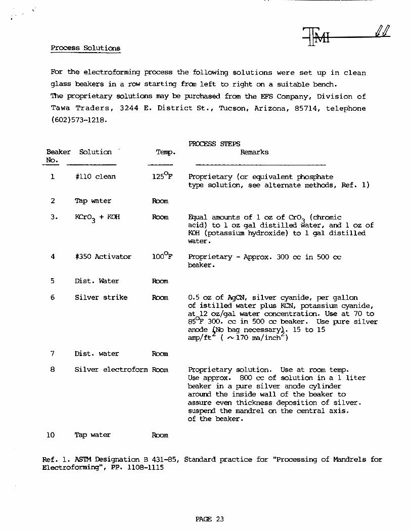
Process Solutions

For the electroforming process the following solutions were set up in clean glass beakers in a row starting fran left to right on a suitable bench.

The proprietary solutions may be prchased from the EFS Company, Division of Tawa Traders, 3244 E. District St., Tucson, Arizona, 85714, telephone (602)573-1218.

Beaker Solution No. - 1 #I10 clean

2 T%p water

3. KCr03 + KOH

4

5

6

7

8

10

Ref.

Temp-

125%

Fbom

Fbom

#350 Activator 100%

Dist. Water Fbom

Silver strike Rxm

Dist. water Rxm

Silver electroform k o m

Tap water Eioam

1. Rs?M Designation B 431-85,

PROCESS mps Remarks

Proprietary (or equivalent phosphate type solution, see alternate methods, Ref. 1)

Equal amounts of 1 oz of eo3 (chromic acid) to 1 oz gal distilled water, and 1 oz of KCH (potassium hydroxide) to 1 gal distilled water.

Proprietary -?pprox. 300 cc in 500 cc beaker.

0.5 oz of AgcN, silver cyanide, per gallon of istilled water plus KCN, potassium cyanide, at 12 oz/gal water concentration. Use at 70 to 85% 300. cc in 500 cc beaker. anode $No bag necessary4. 15 to 15 amp/ft ( 6170 ma/inch )

Use plre silver

Proprietary solution. Use approx. 800 cc of solutim in a 1 liter beaker in a pre silver ande cylinder around the inside wall of the beaker to assure even thickness deposition of silver. susperd the mandrel on the central axis. of the beaker.

Use at room temp.

Standard practice for "Processing of Mandrels for Electroforming", PP. 1108-1115

PA= 23

-

Processing Times

The following processing times have been either experimentally determined or calculated. Silver in the electroform solution will deposit at the rate of one mil (0.001") per square inch per hour at a current of 43 millimprs. kom this, the deposition time to deposit a 5 mil (0.005") layer on each of the mandrels may be found. The followirrg list shows the processing times for each beaker step.

Processing Time Step Solution Time

1 #I10 clean 3 minutes 2 Tap water 30 seconds 3 KCr + KOH 10 seconds 4 Dished water 15 seconds 5 Silver strike 60 seconds 6 Distilled water 15 seconds 7 Silver electroform By timer, see times below 8 Tap water 15 seconds

Deposition Rate of Silver

Silver deposits at the rate of 4.03 gm per ampere bur. At this rate the qproximate ampere burs for deposition of the mandrels #1 through #6 was determined. The time required was then be calculated as determined by the current used.

Mandrel Area in # sq. "

1 1.25 2 1.62 3 4.34 4 4.64 5 0.84 6 0.94

using 0.1 amp/square

Area

%I*

8.06 10.44 27.98 29.90 5.43 6.07

inch :

Grams hpers of Silver €burs

1.08 0.27 1.39 0.35 7.47 1.85 7.98 1.98 0.72 0.18 1.61 0.40

Deposit time at time at 0.1

21 8m 2h 8m 4h 16m 4h 16m 2h 8m 4h 16m

Ampere Hours 1/10 area in sq 'I

Deposit Time =

PAa 24

For other currents as may be required:

Remval of WorkDiece from Mandrel

The use of a passivated stainless steel mandrel together with the use of an approximate two angular degree draft on long parts of the mandrel permited easy removal of the workpiece. In order not to damage the very thin workpiece by Ijhysical removal from the mmdrel,was used to aid in the process. This was done as follows:

After first removing the hangar rod and the stop off insulating washers, a long (possibly 8 to 10 inch) rod of stainless steel with thermally insulating handle was screwed into the tam hole used for the hangar. Holding the mandrel by this handle (with glove protected hand) the mandrel was inserted into a furnace which had been preheated to approximately 1600%. After a few seconds the silver electroform was heated from radiatim and expanded. A slight "pop" was heard as the inner surface of silver part parts from the stainless steel mandrel. This differential expansion takes place since the poor heat oonductivity of the stainless causes the silver to expand more rapidly relative to the stainless. After the electroform was loose on the mandrel it was subsequently annealed under controlled conditions.. The removed electroform part was handled ard packaged with care to prevent damage

B. Printed/Deposited Thermopiles

The second manufacturing technique which we have explored is the use of thin film (printed circuit) technology for increasing the number of thermocouple pairs in the sensor thermopile. At present, the use of fine wire, chrmel-constantan oouples (which are spot welded and applied Over the thermal resistor of the cavity sensor) limit the sensitivity whidh m y be achieved using a reasonable number of junctions. Forty eight junction pairs compose the standard cavity assedly. With photo lithography techniques and thin film etching, the number of junctions in a given space will be significantly increased thus increasirq sensor sensitivity. A factor of 3 to 4 increase in number of junctions has been shown to be feasible. The company now working with us on this problem and w h o we expect to produce an exceptional printed

PAa 25

T 1

n

circuit thermopile is Micro Engineering 11, 14 N. Benson Ave., Upland, California, 91786, telephone (714) 946-2110. AT": John Hall.

VI. Test Item Manufacture

From subcontract i tem suppliers electroformed parts ard printed/deposited thermopiles for t w types of test cavity asseblies were ordered. In both cases, TMI personnel had to interact with the supplier in order to get parts which meet our requirements. Additionally, the cavity mounting disks were machined, and miscellaneous radianeter body a d test apparatus were modified for use in the test radiometers and testing.

The cavities assemblies were fabricated through a process previously described. The thermopiles were installed on the cavity assemblies by techniques standard in strain gage installations. That is, 610 cement was used with the thermopile held in place under pressure and the adhesive cured in an oven at elevated temperature. Lead wires were attached to solder pads on the thermopile sheet. ?he cavity was then installed in a test radiometer body. Sufficient test radiometers aril apparatus were fabricated to support the test program required to verify the sensitivity and time constant predictions.

VII. Test Program

The test program consisted of t m parts for each cavity type. First, response time was measured. QI the test radiometer was installed a high speed shutter. The radiometer was then mounted on a tracker indexed on the sun. A "fast response" XY recorder was hooked up to the thermopile leads. After adjustment and stabilization, and with a "steady sun" the shutter was tripped and the response recorded. This type test was performed a number of times for each cavity type. When repeatability of response time measurement was demonstrated, the test series was terminated and the next test performed.

The sensitivity measurement test required more rigorous test control. For these tests, a measurement of the incoming solar radiance is required. The TMI Standard Instrument, Mk VI S/N 67401, was also installed on the tracker.

PAGE 26

Simultaneous measurements of incoming irradiance and radiometer response recorded. These test were repeated until repeatablility was demonstrated.

The test equipment used are as follows:

1. Cbuld Series 60000 XY recorder, S/N 052134 Main kame

Writing speed: 12Ocm/sec in Y axis, 60cm/sec in X axis Slew speed: 134cm/sec Linearity: M.l% f.s.d. Repeatability: S.l% f.s.d.

X & Y Input Amplifiers Input impedance: IMeg ohm Sensitivity: 18 ranges from O.OSmV/cm to 20.OV/cm

Speeds: 8 ranges from 0.1 to 2O.Osec/cm Accuracy: lt18 f.s.d. Linearity: fl% f .s.d.

Time Base

2. mta Precision Digital Multimeter, W e 1 3600, S/N 1678 Specifications for .2V range

Resolution : luV Input Impedance: >lOOOMeg ohm Accuracy: 24Hr: @23OC + loC,*(0.005% inp. + 4 1.s.d.) cormnxl Mode Rejection Ratio: 160 dB at dc with 1000 ohm

Unbalance

3. Technical Measurements Radiometer Control Unit, Mk I, S/N 47302 Specifications h e n used with hk VI Radiomenter

Accuracy: Absolute measurement uncertainty is less than

Zero Drift: <H.1% / mnth of ?MI radiometer full raqe Time Constant: <2 seconds (l/e) Readirqs in Absolute Energy Units

Ita. 5% of the ?MI radiometer range

RESULTS OBTAINED

PAGJ3 27

w I. Analysis and Manufacturing Results

Our analysis indicates two principal things. First, the required time constant for the cavity sensor is probably longer than the requirement statement of t m seconds, and secord, a cavity sensor with a time constant of less than t m secords can be designed that will have the required sensitivity. The parameter chart given in Figure 3, page 16, shows that one can trade time constant for sensitivity. Because a cavity can be designed with a time constant of significantly less than two secords, consideration can be given to adding an electric heater to the cavity cone for self calibration. The added mass of the heater can be tolerated with a corresponding increase in response time Without undue reduction in sensitivity.

In the manufacturing phase of the work, good success was obtained in the electro-forming of the cavity parts in silver. The density of the deposited silver was close to that of sheet stock and good control of thicknes was achieved. Eb problems in fillet buildup or thin spots occured when proper procedures were followed. Clearly, electroforming of the cavity sensor parts yield the satisfactory silver parts for the cavity sensor. The assembly process using oven solderirrg techniques worked well.

Sufficient silver cavity parts and muper munting rings were fabricated for assembly of test cavities of two types: the standard Kendall design (designated PR for PACRAD radiometer) modified for the new manufacturing method, and the new design for high sensitivity and fast response (designated Em).

The fabrication of the thermopiles was an entirely different matter. We first had to back away from antimony-bismuth thermocouples because no R&D

fabricators were available who could handle the health/safety hazards associated with these materials. It then became apparent that while all the fabrication steps needed to produce a successful thermopile had been developed and used in the fabrication of other products, the combination of them in producing a single product had not been done. The dimensional stability of the Kapton during the fabrication processes caused problems in the adhesion of the thermocouple material and registration of the patterns of the two materials. Improved control of ambient temperature and holding tension of the

PAGE 20

Kapton should cure this problem. To make the thermocoule junction, it is necessary to vacuum deposite a second material on to a plate whidh is then thin film etched to develop the desired wire pattern. The resulting wire pattern is then transfered with proper registration to the Kapton sheet containing the first material. In this process, difficulty was experienced in the release of the thermocouple material fran the Teflm backing material. The cause of this is m t known at this time, but it is probably caused by surface activation of the Teflon during the vacuum deposition process. This technique has been successful in other applications.

In the many attempts made to fabricate the thermopiles, partial successes were achieved but m functioning thermopiles were obtained. Additional developent work is required which will take many months. ?lo continue the developent work on the cavities, and allow estimates of performance to be made, we resorted to building thermocouples and thermopiles out of small (36 gauge. 0.005" diameter) thermocouple wire.

11. Test Results

A. Sensitivity

The test results of the measured sensitivity in ambient air are quite god. The cavities were instrumented with 14 junction thermopiles made out of wire and mounted on Kapton insulation. The measured results were then ratioed up by a factor of 174/14 to account for the fewer junctions of the wire thermopile. The Kendall standard design (PR) indicated a sensitivity of 32 uv/(mw/cm ) and the high sensitivity fast response design indicated 60 uv/(m/an2). In vacuum, the sensitivity should increase approximately 30%. The sensitivity of the HSFR cavity exceeds the requirement statement of 0.02'

2 (mw/cm )/uv. The PR cavity would just meet the requirement in vacuum

2

(space).

B. Response Time

The nature of the 14 junction thermopile used for making the sensitivity measurements, preclude making short response time measurements. Because of the thermal insulation of the Kapton and the relative massiveness of the

PAGE 29

wires, the measured time constant is dominated by the response time of the thermopile. This is evident in the measurements of response time for the two cavity types when instrumented with the 14 junction thermopiles. The PR cavity exhibited a response time 2 . 3 seconds, while the HSFR cavity showed a respanse time of 3 . 4 seconds. The installation of the thermopile is more difficult on the HSFR cavity and resulted poorer thermal conductivity at the junctions to the silver thermal resistor. Tb Overcome this problem, a single thermocouple junction was attached by solder to the thermal resistor with as small a bead as possible. Fbr good attachment, the resulting bead size was 0.02". With this thermocouple, the response time of the HSFR cavity was measured to be 1.85 seconds. !this meets the requirement statement of less than two seconds.

111. Performance Estimates

The test results obtained in the resear&, to this time, are ccanpramised by the lack of an adequate thermopile. ?he bead size used with the HSFR cavity determined the measured time constant. The Omega Temperature measurement Handbook and Ehcyclopedia provides data on response time verses bead size. This data suggests a thermocouple junction of the size we used to about 1.4 seconds. It also suggests that a reduction in size to our target size of 0.003'' wxld result in a junction time constant of less than 0.1 seconds. The overall time constant of the cavity sensor would then be very close to the time constant of the silver parts. Based on these considerations, we estimate

2 that a JSFR cavity can be produce With a sensitivity of 0.02 (m/cm /uv) with a time constant of less than t m semds.

ESTIMATE C F TECHNICAL FEASIBILITY

In the short time TMI had to conduct this researdh, it was necessary to make estimates of the desired characteristics of the sensor and then to build models which thorough testing would demonstrate the design principles and allow predictions of performance. From that base, the design of optimum sensors for the specific ACAI missim can be developed. The results of the Phase I work Shows that cavities tailored to the specific requirements of each ring of the ACAI can be provided.

PAGE 30

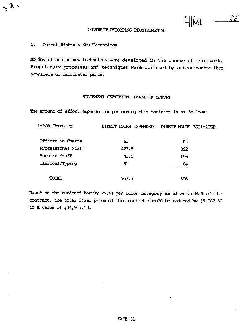
I. Patent Rights & New Technology

No inventions or new technology were developed in the course of this work. Proprietary processes and techniques were utilized by subcontractor item suppliers of fabricated parts.

The m u n t of effort expended in performing this contract is as follows:

Officer in Charge Professional Staff mpport Staff Clerical /mi ng

51 423.5 41.5 51

TcnaL 567.5

DIRECT €DLJRS ESTIMATED

84

392 156 64

696

Based cn the burdened burly rates per labor category as show in H. 5 of the contract, the total fixed price of this contact sbuld be reduced by $5,082.50 to a value of $44,917.50.

PAGE 31