61

Fatigue Load Computation of Wind TurbineGearboxes by Coupled Structural, Mechanism and Aerodynamic Analysis

A. Heege, Y. Radovcic, J. Betran, SAMTECH Iberica. www.samcef.com

DEWI Magazin Nr. 28, Februar 2006

Introduction

With a service life of about 20 years, wind turbine power trains are subjected to a very diverse spectrumof dynamic loads. Due to the high number of load cycles which occur during the life of the turbine, fatigueconsiderations are of particular importance in wind turbine design. Power train bearing failures occurmore frequently than damage to the other components. Taking into account that these failures occur toa certain degree after a couple of years of successful operation, the importance of proper fatigue con-siderations becomes obvious.

The respective load spectrum, in terms of load amplitudes and associated load cycles, depends on thedynamic properties of the complete mechatronical wind turbine system and cannot be calculated prop-erly without detailed three-dimensional models. “External excitations” in terms of “aerodynamic bladeloads” and “electromagnetic generator torques”, depend implicitly on control strategies for blade pitchand/or generator electronics, as well as on the general dynamic properties of the whole turbine. Thepurely dynamic character of certain gearbox loads, such as that on the planet carrier bearings, stressesthe need for detailed dynamic power train models, which reproduce load frequencies and amplificationsof the individual gearbox components with sufficient precision.

Widely used procedures for fatigue evaluation of gearbox loads rely essentially on the load history of therotor main shaft and account only partially for the three-dimensional character of dynamic power trainloads. Experimental measurements and numerical simulations have shown that dynamic load amplifica-tions within the gearbox can be much larger than those calculated from measurements of rotor or highspeed shaft torque transients.

New standards for design and specification of gearboxes for wind turbines, like the American nationalstandard “AGMA 6006-A03”, requires all dynamic effects be included in the fatigue load computation. Inorder to cope with these requirements, the proposed fatigue procedure relies on a complete mechatron-ical wind turbine model, which includes a detailed gearbox model. Accordingly, the load transients areextracted from the global model for each gearbox component and fatigue cycle counting is performedindividually for each power train component. This procedure has the advantage that the frequency con-tent and the associated amplitudes of the local transients account for the non-linear character of dynam-ic amplifications within the power train and respect the implicit dependence of the excitations on thedynamic properties of the entire mechatronical system. The fatigue load spectra, which are obtainedfrom the global wind turbine model in terms of “component wise load transients”, account for localdynamic effects within the gearbox as well.

Various topics will be dealt with as follows: section 1 is a brief summary of the mathematical approachfor coupling the Finite Element Method (FEM), mechanisms, control loops and finally aerodynamics interms of “Aerodynamic Blade Section Elements”. In section 2 the aerodynamic-mechatronical wind tur-bine model is presented. In section 3 some aerodynamic results are shown for an emergency stop.Numerical results are compared to experimental and detailed results are shown for a gearbox with twoplanetary stages. A “grid loss event” with subsequent emergency stop has been chosen as an example,in order to present dynamic load amplifications separately for each bearing and gear. Component-wisefatigue diagrams are exposed in section 4 and finally in section 5 the conclusions are presented.

1. Coupling Mechanism, Structural Analysis and Aerodynamics

Augmented Lagrangian approach

In order to introduce the mathematical background of the coupled field problem, we start from classicalnon-linear Finite Element Method (FEM) equation:

Externer Artikel

62

In equation (1), stiffness matrix , damping matrix and of the right hand side shownon-linear dependency on the solution vector . As follows, the matrix equation (1) will be extendedin order to account for mechanisms, like for example, gears, control loops, or aerodynamic followerforces. These additional equations are introduced adopting an Augmented Lagrangian /4,5/. The finalexpression of the Augmented Lagrangian is stated in equation (2) for a given time step “n”, where thenon-linear FEM equations are included in the vector . Final discretized equilibrium equation of thecoupled field problem is modified by the “Hilber Hughes & Taylor” form (HHT) /2/ in order to improvethe numerical stability in presence of constraints . The factor k is a scaling factor associated with

the constraints in order to improve numerical conditioning, , the transposed vector of the con-straint gradients and α is a factor introduced by the HHT modification.

Equation (2) represents the equilibrium state of coupled structures (FEM), mechanisms (MBS), controlloops and aerodynamics for a given time instance /8/. The generalized solution vector , yields the glob-al solution of the coupled field problem, in terms of “FEM nodal variables”, MBS state variables, andaerodynamic forces. Further details on time integration procedure, error estimators, or solution strategy for equation solvers,can be found in the SAMCEF Mecano user manual /8/.

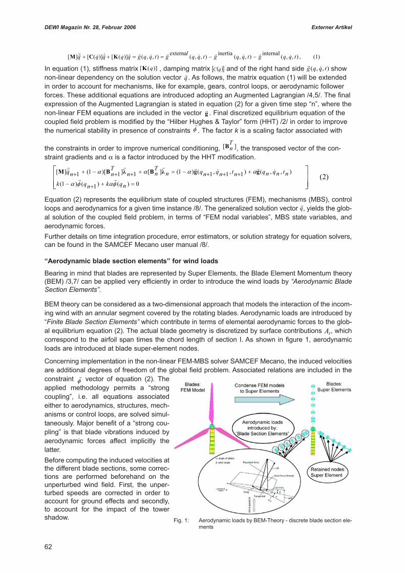
“Aerodynamic blade section elements” for wind loads

Bearing in mind that blades are represented by Super Elements, the Blade Element Momentum theory(BEM) /3,7/ can be applied very efficiently in order to introduce the wind loads by “Aerodynamic BladeSection Elements”.

BEM theory can be considered as a two-dimensional approach that models the interaction of the incom-ing wind with an annular segment covered by the rotating blades. Aerodynamic loads are introduced by“Finite Blade Section Elements” which contribute in terms of elemental aerodynamic forces to the glob-al equilibrium equation (2). The actual blade geometry is discretized by surface contributions , whichcorrespond to the airfoil span times the chord length of section I. As shown in figure 1, aerodynamicloads are introduced at blade super-element nodes.

Concerning implementation in the non-linear FEM-MBS solver SAMCEF Mecano, the induced velocitiesare additional degrees of freedom of the global field problem. Associated relations are included in theconstraint vector of equation (2). Theapplied methodology permits a “strongcoupling”, i.e. all equations associatedeither to aerodynamics, structures, mech-anisms or control loops, are solved simul-taneously. Major benefit of a “strong cou-pling” is that blade vibrations induced byaerodynamic forces affect implicitly thelatter. Before computing the induced velocities atthe different blade sections, some correc-tions are performed beforehand on theunperturbed wind field. First, the unper-turbed speeds are corrected in order toaccount for ground effects and secondly,to account for the impact of the towershadow.

IA

q

)2(0)()1()1(

),,()1,1,1()1(][1]1)[1(1][

nqknqk

ntnqnqntnqnqnTnn

Tnnq ggBBM

][TnB

g

q

),,( tqqgqC)]([ qK

(1) , ),,(internal

),,(inertia

),,(externa

),,()]([ )]([][ tqqgtqqgtqql

gtqqgqqqqq KCM

DEWI Magazin Nr. 28, Februar 2006

Fig. 1: Aerodynamic loads by BEM-Theory - discrete blade section ele-ments

Externer Artikel

Since aerodynamic torque is potentiallyhigher than generator resistive torque andunsteady wind is considered, a pitch con-trol is necessary to stabilize the machine atreasonably constant speed.

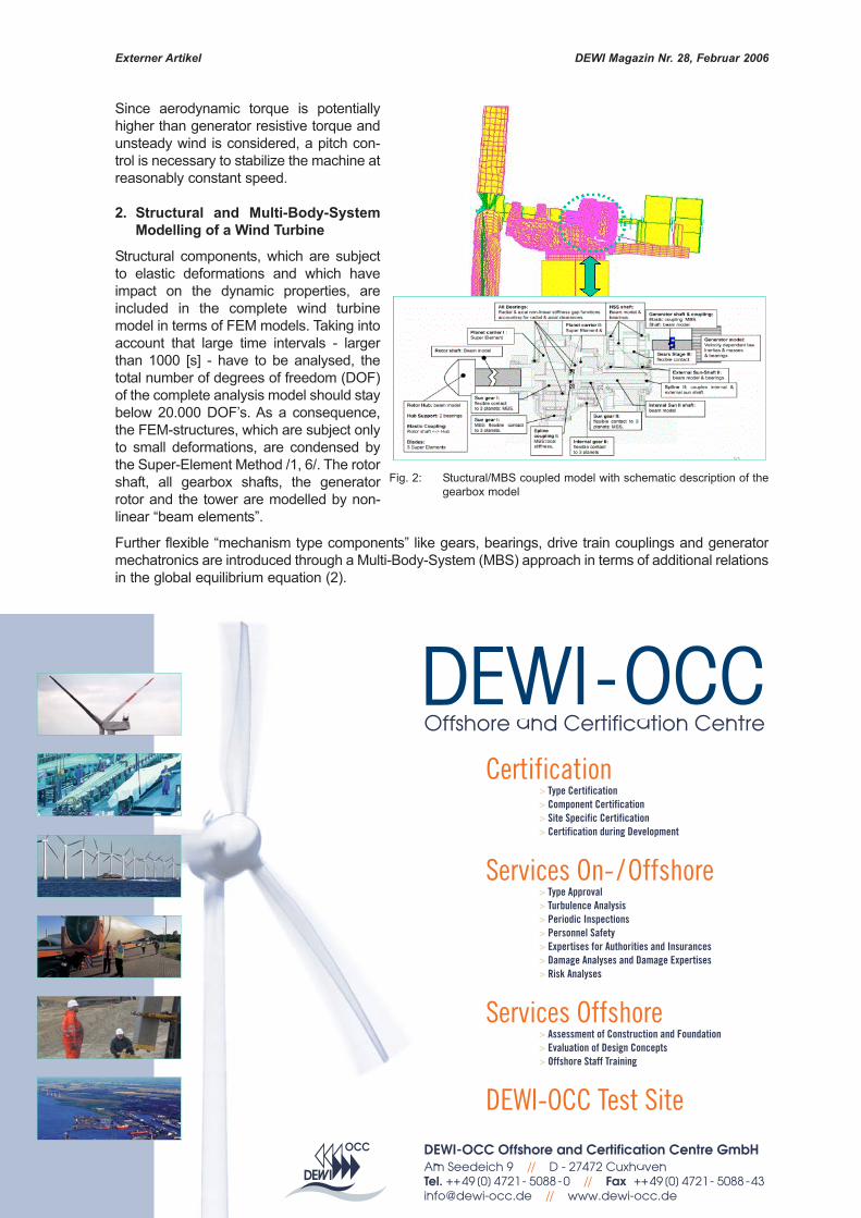
2. Structural and Multi-Body-SystemModelling of a Wind Turbine

Structural components, which are subjectto elastic deformations and which haveimpact on the dynamic properties, areincluded in the complete wind turbinemodel in terms of FEM models. Taking intoaccount that large time intervals - largerthan 1000 [s] - have to be analysed, thetotal number of degrees of freedom (DOF)of the complete analysis model should staybelow 20.000 DOF’s. As a consequence,the FEM-structures, which are subject onlyto small deformations, are condensed bythe Super-Element Method /1, 6/. The rotorshaft, all gearbox shafts, the generatorrotor and the tower are modelled by non-linear “beam elements”.

Further flexible “mechanism type components” like gears, bearings, drive train couplings and generatormechatronics are introduced through a Multi-Body-System (MBS) approach in terms of additional relationsin the global equilibrium equation (2).

DEWI Magazin Nr. 28, Februar 2006

Certification> Type Certification> Component Certification> Site Specific Certification> Certification during Development

Services On- /Offshore> Type Approval> Turbulence Analysis> Periodic Inspections> Personnel Safety> Expertises for Authorities and Insurances> Damage Analyses and Damage Expertises> Risk Analyses

Services Offshore> Assessment of Construction and Foundation> Evaluation of Design Concepts> Offshore Staff Training

DEWI-OCC Test Site

Offshore and Certification Centre

DEWI-OCC Offshore and Certification Centre GmbHAm Seedeich 9 // D - 27472 CuxhavenTel. ++49[0] 4721- 5088 -0 // Fax ++49[0] 4721- 5088 -43info@dewi-occ.de // www.dewi-occ.de

Fig. 2: Stuctural/MBS coupled model with schematic description of thegearbox model

Externer Artikel

64

Gearbox Modelling: Coupled MBS & FEM Approach

Gearbox is included in the global analysis model combining FEM and MBS approach /9,10,11/. As writ-ten, all gearbox shafts are represented by non-linear beam elements. Gearbox housing is modelled by asolid FEM model, which is condensed to a Super Element in order to reduce the number of degrees offreedom.

The frictional contact problems between flexible gears are reduced to geometrically variable, and pointwise flexible contacts. Gear geometry is defined by helix-, cone- and pressure angles, normal modulus,respective teeth number and, if needed, further correction factors for the gear teeth. Gear teeth flexibilityis defined either according to ISO 6336, or by non-linear gap-functions. It is emphasized that the propermodelling of gear and bearing clearances is of crucial importance when evaluating gearbox loads duringbacklashes.

Every bearing of the wind turbine, including the rotor main shaft, the entire gearbox and the generator, ismodelled by non-linear stiffness functions, which account for the coupling of radial and axial bearing prop-erties. All bearing clearances in radial and axial directions are accounted for. If detailed stress computa-tion is required, frictional contact between bearing components, or between gears is modelled by fullynon-linear FEM models.

Generator and Controllers

The electro-mechanical generator characteristics are defined in terms of non-linear “torque versus speed”functions. This non-linear “generator function” may be modified during certain operation modes due tocontrol actions, or in order to simulate grid failures. It is emphasized that the resulting transient generatortorque is an analysis result and not a boundary condition. Note that general control loops are definedeither directly using the controllers implemented in SAMCEF®, or can be imported from Matlab/Simulink®controller models.

3. Application Examples

Emergency stop: aerodynamic results

Our first numerical example is an emer-gency stop simulation. Emergency stopor E-stop, is the process that bring thewind turbine to idle as fast as possible.The E-stop is commanded by the controlsystem in determined cases: grid loss,excessive vibrations,...

Figure 2 shows a typical “Numerical WindTurbine Model” including on one handstructural “FEM Components” like blades,rotor- and gearbox shafts, tower struc-ture, gearbox housing, planet-carrier,bedplate etc. and on the other hand “MBStype components” like gears, bearings, elastic couplings or bushings, overload clutch, and finally the gen-erator model & control loops. As depicted schematically in figure 2, the gearbox model is based on twoplanetary stages and one parallel helical stage where the numerical model accounts for every relevantgearbox components.

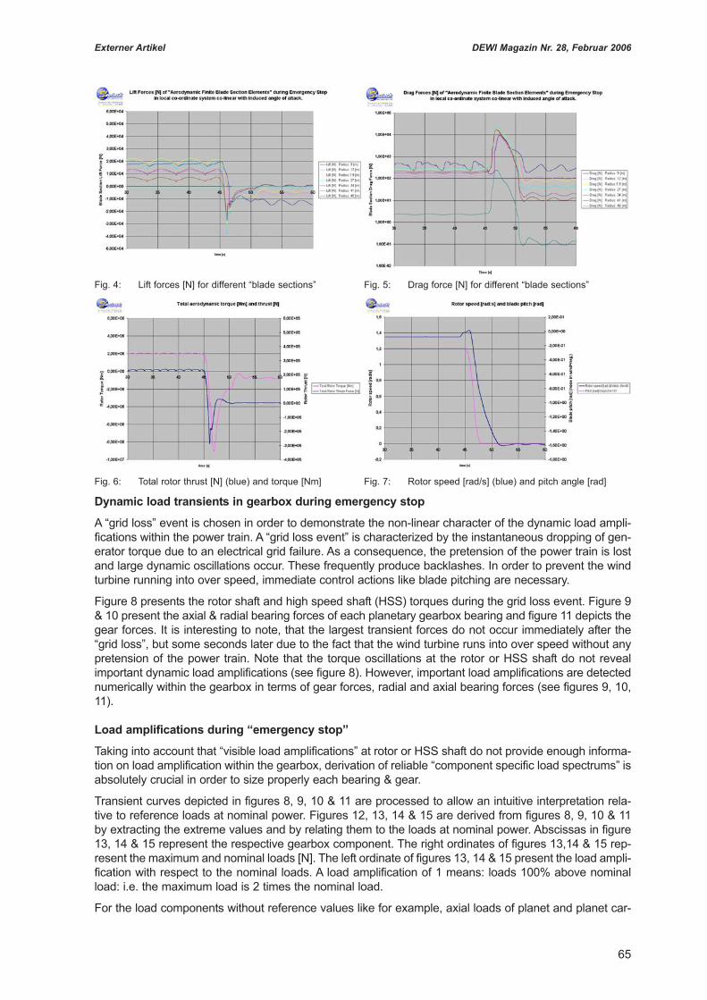
Aerodynamic loads are entered through the finite aerodynamic blade elements. Figure 3 shows lift, dragand moment coefficients for some blade sections. In this simulation, wind turbine runs at constant wind of15 m/s. The generator disconnects at 44 [s]. The disk brake located at gearbox exit starts acting immedi-ately but reaches full power after some tenths of a second. Blades are pitched “in the wind” at the sametime to bring turbine to rest (figure 7, pink curve referring to right ordinate). As shown in figure 7, bladepitch is nearly constant up to time 45 [s] and turned in the following seconds 90 [degrees] into the wind inorder to invert the rotor torque.

Figures 4 and 5 show the lift and drag forces acting on one blade at different radii. Figure 6 shows theresulting total aerodynamic torque and total thrust during the whole process. Note that the effect of windshear and tower shadow are considered and the latter is visible in figures 4, 5 & 6.

DEWI Magazin Nr. 28, Februar 2006

Fig. 3: Lift, drag and moment coefficients for some blade sections

Externer Artikel

Dynamic load transients in gearbox during emergency stop

A “grid loss” event is chosen in order to demonstrate the non-linear character of the dynamic load ampli-fications within the power train. A “grid loss event” is characterized by the instantaneous dropping of gen-erator torque due to an electrical grid failure. As a consequence, the pretension of the power train is lostand large dynamic oscillations occur. These frequently produce backlashes. In order to prevent the windturbine running into over speed, immediate control actions like blade pitching are necessary.

Figure 8 presents the rotor shaft and high speed shaft (HSS) torques during the grid loss event. Figure 9& 10 present the axial & radial bearing forces of each planetary gearbox bearing and figure 11 depicts thegear forces. It is interesting to note, that the largest transient forces do not occur immediately after the“grid loss”, but some seconds later due to the fact that the wind turbine runs into over speed without anypretension of the power train. Note that the torque oscillations at the rotor or HSS shaft do not revealimportant dynamic load amplifications (see figure 8). However, important load amplifications are detectednumerically within the gearbox in terms of gear forces, radial and axial bearing forces (see figures 9, 10,11).

Load amplifications during “emergency stop”

Taking into account that “visible load amplifications” at rotor or HSS shaft do not provide enough informa-tion on load amplification within the gearbox, derivation of reliable “component specific load spectrums” isabsolutely crucial in order to size properly each bearing & gear.

Transient curves depicted in figures 8, 9, 10 & 11 are processed to allow an intuitive interpretation rela-tive to reference loads at nominal power. Figures 12, 13, 14 & 15 are derived from figures 8, 9, 10 & 11by extracting the extreme values and by relating them to the loads at nominal power. Abscissas in figure13, 14 & 15 represent the respective gearbox component. The right ordinates of figures 13,14 & 15 rep-resent the maximum and nominal loads [N]. The left ordinate of figures 13, 14 & 15 present the load ampli-fication with respect to the nominal loads. A load amplification of 1 means: loads 100% above nominalload: i.e. the maximum load is 2 times the nominal load.

For the load components without reference values like for example, axial loads of planet and planet car-

65

DEWI Magazin Nr. 28, Februar 2006

Fig. 4: Lift forces [N] for different “blade sections” Fig. 5: Drag force [N] for different “blade sections”

Fig. 6: Total rotor thrust [N] (blue) and torque [Nm] Fig. 7: Rotor speed [rad/s] (blue) and pitch angle [rad]

Externer Artikel

66

rier bearings, there is no reference value and loads are of purely dynamic nature. In that case, we showaverage dynamic loads at nominal power and maximum dynamic loads occurring during and after theevent. It is crucial to recognize that the load amplifications within the gearbox are much larger than theamplifications which would be detected by experimental measurement or numerical simulation at rotorshaft and/or HSS shaft.

Comparison of numerical results to experiment

Figure 16 shows the comparison of the numerical rotor shaft torque results to the corresponding experi-mental data during an emergency stop at low wind conditions. The sudden augmentation of rotor shafttorque at about time =6[s] is due to the activation of the disc brake at the gearbox exit. It can be seen thatthe numerical model reproduces with a very satisfactory precision the “system change” which occurs atthe transition from “braking” to “turbine at idle”. During the time interval [6s – 10 s] “first drive train mode”is visible at about 1.1 [Hz]. At about time [10 s], the turbine starts idling and the dominating frequencydrops to about 0.5 [Hz]. Figure 16 also includes a zoom on one single oscillation at turbine idle. The com-parison to experimental data shows that the numerical model reproduces properly the “zero torqueinstances” due to clearances.

4. Fatigue Evaluations

In widely used design practices of gearboxes, fatigue evaluations are based essentially on the time his-tory of the rotor shaft torque. Looking at the transient curves depicted in figures 8-11, it can be seen thatthis design practice is only of very limited precision. Better load spectra for the different gearbox compo-nents are obtained, if the non-linear dynamic load amplifications are introduced component wise to cor-rect the input rotor shaft time histories. However, this approach only corrects load amplitudes seen bycomponent, but not the associated load frequencies.

Further improvement to fatigue load spectra of power train components is obtained by extracting RainFlow Counting (RFC) and Load Duration Distributions (LDD) separately for each gearbox component. Inthis approach, transient loads are extracted for each power train component from the global mechatroni-

DEWI Magazin Nr. 28, Februar 2006

Fig. 8: Rotor & HSS shaft torques [Nm] Fig. 9: Axial bearing forces [N]

Fig. 10: Radial bearing forces [N] Fig. 11: Gear forces [N]

Externer Artikel

cal wind turbine model and, RFC and/or LDD areperformed separately for each bearing and gear.Thus, fatigue load spectra account as well for localdynamic effects within the gearbox. As a conse-quence, load cycles of higher frequency content areincluded in the fatigue spectra. Furthermore, dynam-ic amplifications of operation states producing localresonance are taken into account.

In the case of structural components, FEM modelsmight be used in order to compute the stress stateassociated with each load cycle and correspondingload case. Structural components like blades or bed-plate are included in the global model, but condensed by the Super Element Method to reduce CPU time.Stress within these components can be recovered at any instance of the transient analysis, by a back-transformation from the condensed Super Element. Damage can then be computed from this stress his-tory. Bearings and gears are modelled by a MBS approach, thus reducing the analysis results to three-dimensional load transients. Theses load transients might be used as boundary conditions for detailedFEM models. However it might be more convenient to use instead analytical methods in order to deducerespective component damage from RFC results.

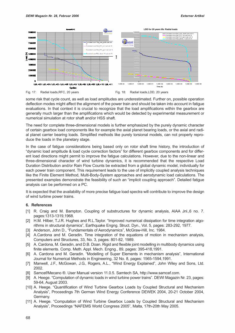
Figure 17 presents individually for each bearing the radial bearing load cycles in terms of RFC’s obtainedby gathering relevant load cases over 20 years of operation. Analogously, figure 18 presents the “cumu-lated radial bearing load duration distribution” (LDD) for 20 years of operation.

5. Conclusions

The implicit dependence of “power train loads” on the dynamic characteristics of the assembled wind tur-bine, excludes a decoupling of analysis techniques, in order to reduce the complexity of the numericalmodels. If a gearbox is analyzed without accounting for the other properties of the wind turbine, there is

67

DEWI Magazin Nr. 28, Februar 2006

Fig. 12: Torques & speeds of rotor & HSS shafts Fig. 13: Axial bearing loads

Fig. 14: Gear loads Fig. 15: Radial bearing loads

Fig. 16: Comparison to experiment, Main shaft torque [Nm].

Externer Artikel

68

some risk that cycle count, as well as load amplitudes are underestimated. Further on, possible operationdeflection modes might affect the alignment of the power train and should be taken into account in fatigueevaluations. In that context it is crucial to recognize that the load amplifications within the gearbox aregenerally much larger than the amplifications which would be detected by experimental measurement ornumerical simulation at rotor shaft and/or HSS shaft.

The need for complete three-dimensional models is further emphasized by the purely dynamic characterof certain gearbox load components like for example the axial planet bearing loads, or the axial and radi-al planet carrier bearing loads. Simplified methods like purely torsional models, can not properly repro-duce the loads in the planetary stage.

In the case of fatigue considerations being based only on rotor shaft time history, the introduction of“dynamic load amplitude & load cycle correction factors” for different gearbox components and for differ-ent load directions might permit to improve the fatigue calculations. However, due to the non-linear andthree-dimensional character of wind turbine dynamics, it is recommended that the respective LoadDuration Distribution and/or Rain Flow Counts be extracted from a global dynamic model, individually foreach power train component. This requirement leads to the use of implicitly coupled analysis techniqueslike the Finite Element Method, Multi-Body-System approaches and aerodynamic load calculations. Thepresented examples demonstrate the feasibility of such an “implicit coupling approach”. Detailed fatigueanalysis can be performed on a PC.

It is expected that the availability of more precise fatigue load spectra will contribute to improve the designof wind turbine power trains.

6. References[1] R. Craig and M. Bampton. Coupling of substructures for dynamic analysis, AIAA Jnl.,6 no. 7.

pages:1313-1319,1968.[2] H.M. Hilber, T.J.R. Hughes and R.L.Taylor. “Improved numerical dissipation for time integration algo-

rithms in structural dynamics”, Earthquake Engng. Struct. Dyn., Vol. 5, pages: 283-292, 1977.[3] Anderson, John D., “Fundamentals of Aerodynamics”, McGraw-Hill, Inc. 1984.[4] A.Cardona and M. Geradin. Time integration of the equations of motion in mechanism analysis,

Computers and Structures, 33, No. 3, pages: 801-82, 1989.[5] A. Cardona, M. Geradin, and D.B. Doan. Rigid and flexible joint modelling in multibody dynamics using

finite elements. Comp. Meth. Appl. Mech. Engng., 89, pages: 395-418,1991.[6] A. Cardona and M. Geradin. “Modelling of Super Elements in mechanism analysis”, International

Journal for Numerical Methods in Engineering, 32 No. 8, pages: 1565-1594,1991.[7] Manwell, J.F., McGowan, J.G., Rogers, A.L., “Wind Energy Explained”, John Wiley and Sons, Ltd.

2002.[8] Samcef/Mecano ®. User Manual version 11.0.5. Samtech SA, http://www.samcef.com.[9] A. Heege. “Computation of dynamic loads in wind turbine power trains”. DEWI Magazin Nr. 23, pages:

59-64, August 2003.[10] A. Heege. “Quantification of Wind Turbine Gearbox Loads by Coupled Structural and Mechanism

Analysis”, Proceedings 7th German Wind Energy Conference DEWEK 2004, 20-21 October 2004,Germany.

[11] A. Heege. “Computation of Wind Turbine Gearbox Loads by Coupled Structural and MechanismAnalysis”, Proceedings “NAFEMS World Congress 2005”, Malta, 17th-20th May 2005.

DEWI Magazin Nr. 28, Februar 2006

Fig. 17: Radial loads,RFC, 20 years Fig. 18: Radial loads,LDD, 20 years

0

100000

200000

300000

400000

500000

600000

700000

800000

900000

1000000

1,00E-02 1,00E-01 1,00E+00 1,00E+01 1,00E+02 1,00E+03 1,00E+04 1,00E+05 1,00E+06

Time (h)

Lo

ad

Cumulated count Rad_main_shaft Load unit: NCumulated count Rad_PLC_rot Load unit: NCumulated count Rad_PLC_gen Load unit: NCumulated count Rad_planet_1 Load unit: N

LDD for 20 years life: Radial loads

Externer Artikel