Measuring Risk

Ch 2 Chapter 8 ( Interest Rate Risk )

( How can you measure Interest Rate Risk)

1- INTRODUCTION In Chapter 7 we established that while performing their asset-transformation functions, FIs often mismatch the maturities of their assets and liabilities. In so doing, they expose themselves to interest rate risk. For example, in the 1980s a large number of thrifts suffered economic insolvency (i.e., the net worth or equity of their owners was eradicated) when interest rates unexpectedly increased. All FIs tend to mismatch their balance sheet maturities to some degree. However, measuring interest rate risk exposure by looking only at the size of the maturity mismatch can be misleading. The next two chapters present techniques used by FIs to measure their interest rate risk exposures.

This chapter begins with a discussion of the Federal Reserve’s monetary policy, which is a key determinant of interest rate risk. The chapter also analyzes the simpler method used to measure an FI’s interest rate risk: the repricing model .

The repricing, or funding gap, model concentrates on the impact of interest rate changes on an FI’s net interest income (NII), which is the difference between an FI’s interest income and interest expense. Because of its simplicity, smaller depository institutions (the vast majority of DIs) still use this model as their primary measure of interest rate risk. Appendix 8A, at the book’s Web site ( www.mhhe .com/saunders6e ), compares and contrasts this model with the market value–based maturity model, which includes the impact of interest rate changes on the overall market value of an FI’s assets and liabilities and, ultimately, its net worth.

1

Until recently, U.S. bank regulators had been content to base their evaluations of bank interest rate risk exposures on the repricing model. As explained later in this chapter, however, the repricing model has some serious weaknesses. Recently, the Bank for International Settlements (the organization of the world’s major Central Banks) issued a consultative document 1 suggesting a standardized model to be used by regulators in evaluating a bank’s interest rate risk exposure. Rather than being based on the reprising model, the approach suggested is firmly based on market value accounting and the duration model (see Chapter 9). As regulators move to adopt these models, bigger banks (which hold the vast majority of total assets in the banking industry) have adopted them as their primary measure of interest rate risk. Moreover, where relevant, banks may be allowed to use their own value-at-risk models (see Chapter 10) to assess the interest rate risk of the banking book.

Appendix 8B, at the end of this chapter, looks at the term structure of interest rates that compares the market yields or interest rate on securities, assuming that all characteristics except maturity are the same. This topic is generally covered in introductory finance courses. For students needing a review, appendix 8B isencouraged introductory reading.NoticeNet worth : The value of an FI to its owners; this is equal to the difference between the market value of assets and that of liabilities.

Before we measure interest rates risk, we can see the level and movement of interest rates, in U.S by looking at the central bank’s monetary policy strategy as follows:-

2-THE LEVEL AND MOVEMENT OF INTEREST RATESWhile many factors influence the level and movement of interest rates , it is the central bank’s monetary policy strategy that most directly underlies the level and movement of interest rates that, in

2

turn, affect an FI’s cost of funds and return on assets. The central bank in U.S is the Federal Reserve (the Fed). Through its daily open market operations, such as buying and selling Treasury bonds and Treasury bills, the Fed seeks to influence the money supply, inflation, and level of interest rates (particularly short-term interest rates. Figure 8–1 shows the interest rate on U.S. three-month T-bills for the period 1965–2011. While Federal Reserve actions are targeted mostly at short-term rates (especially the federal funds rate), changes in short-term rates usually feed through to the whole term structure of interest rates.

FIGURE 8–1 Interest Rate on U.S. 91-Day Treasury Bills, 1965–2011

In addition to the Fed’s impact on interest rates via its monetary policy strategy, the increased level of financial market integration

3

over the last decade has also affected interest rates. Financial market integration increases the speed with which interest rate changes and associated volatility are transmitted among countries, making the control of U.S. interest rates by the Federal Reserve more difficult and less certain than before. The increased globalization of financial market flows in recent years has made the measurement and management of interest rate risk a prominent concern facing many modern FI managers. For example Investors across the world carefully evaluate the statements made by Ben Bernanke (chairman of the Federal Reserve Board of Governors) before Congress. Even hints of increased U.S. interest rates may have a major effect on world interest rates (as well as foreign exchange rates and stock prices).

The level and volatility of interest rates and the increase in worldwide financial market integration make the measurement and management of interest rate risk one of the key issues facing FI managers. Further, the Bank for International Settlements has called for regulations that require depository institutions (DIs) to have interest rate risk measurement systems that assess the effects of interest rate changes on both earnings and economic value. These systems should provide meaningful measures of a DI’s current levels of interest rate risk exposure and should be capable of identifying any excessive exposures that might arise (see Chapter 20).

In this chapter and in Chapter 9, we analyze the different ways an FI might measure the exposure it faces in running a mismatched maturity book (or gap) between its assets and its liabilities in a world of interest rate volatility. In particular, we concentrate on three ways, or models, of measuring the asset– liability gap exposure of an FI:1-The reprising (or funding gap) model.2- The maturity model.3- The duration model.

4

In this chapter we study the first Model (The reprising model). That is, measuring the asset– liability gap exposure of an FI:3- THE REPRICING MODEL The repricing, or funding gap, model is a simple model used by small (thus most) DIs in the United States. This model is essentially a book value accounting cash flow analysis of the repricing gap between the interest income earned on an FI’s assets and the interest expense paid on its liabilities (or its net interest income) over a particular period of time. This contrasts with the market value–based maturity and duration models discussed later in this chapter and in Chapter 9.

Repricing gap : The difference between assets whose interest rates will be repriced or changed over some future period (rate-sensitive assets) and liabilities whose interest rates will be repriced or changed over some future period (rate sensitive liabilities).

النموذج ( The repricing, or funding gap, model) شرح In recent years, the Federal Reserve has required commercial banks to report quarterly on their call reports the repricing gaps for assets and liabilities with these maturities:

1. One day.2. More than one day to three months.3. More than three months to six months.4. More than six months to twelve months.5. More than one year to five years.6. More than five years.7.

Under the repricing gap approach, a bank reports the gaps in each maturity bucket by calculating the rate sensitivity of each asset (RSA) and each liability (RSL) on its balance sheet. Rate sensitivity here means that the asset or liability is repriced at or near current market interest rates within a certain time horizon (or maturity bucket). Repricing can be the result of a rollover of an asset or liability (e.g., a loan is paid off at or prior to maturity and the funds are used to issue a new loan at current market rates), or it can occur because the asset or liability is a variable-rate instrument (e.g., a variable-rate mortgage whose interest rate is reset every quarter based on movements in a prime rate).

5

Rate-sensitive asset or liability: An asset or liability that is repriced at or near current market interest rates within a maturity bucket.

Table 8–1 shows the asset and liability repricing gaps of an FI, categorized into each of the six previously defined maturity buckets. TABLE 8–1 Repricing Gap (in millions of dollars)

(1) (2) (3) (4) Assets Liabilities Gaps Cumulative Gap1. One day $ 20 $ 30 $ -10 $ -102. More than one day–three months 30 40 -10 -203. More than three months–six months 70 85 -15 -354. More than six months–twelve months 90 70 +20 -155. More than one year–five years 40 30 +10 -56. Over five years 10 5 +5 0 ------- ---------- $ 260 $ 260

For example, suppose that an FI has a negative $10 million difference between its assets and liabilities being repriced in one day (one-day bucket). Assets and liabilities that are repriced each day are likely to be interbank borrowings on the federal funds or repurchase agreement market (see Chapter 2). Thus, a negative gap (RSA < RSL) exposes the FI to refinancing risk, in that a rise in these short-term rates would lower(decrase) the FI’s net interest income since the FI has more rate-sensitive liabilities than assets in this bucket. In other words, assuming equal changes in interest rates on RSAs and RSLs, interest expense will increase by more than interest revenue. Conversely, if the FI has a positive $20 million difference between its assets and liabilities being repriced in 6 months to 12 months, it has a positive gap (RSA > RSL) for this period and is exposed to reinvestment risk, in that a drop in rates over this period would lower the FI’s net interest income; that is, interest income will decrease by more than interest expense. Specifically, let:

- = Δ = delta ملحوظه

Δ NIIii = Change in net interest income in the ith bucket i

6

GAPi Δ = Dollar size of the gap between the book value of rate-sensitive assets and rate-sensitive liabilities in maturity bucket i Δ Ri = Change in the level of interest rates impacting assets and liabilities in the ith bucket Then: Δ NIIi = (GAP) Δ Ri = (RSAi - RSLi ) Δ Ri هامه معادله In this first bucket, if the gap is negative $10 million and short-term interest rates (such as fed fund and/or repo rates) rise 1 percent, the annualized change in the FI’s future net interest income is: Δ NIIi = (-$10 million) ×.01 = -100, 000

That is, the negative gap and associated refinancing risk resulted in a loss of $100,000 in net interest income for the FI.Refinancing risk: The risk that the cost of rolling over or reborrowing funds will rise above the returns being earned on asset investments.Reinvestment risk: The risk that the returns on funds to be reinvested will fall below the cost of the funds.

Notices ملاحظاتThis approach is very simple and intuitive. Remember, however, from Chapter 7 and our overview of interest rate risk that capital or market value losses also occur when rates rise. The capital loss effect that is measured by both the maturity and duration models developed in the appendix to this chapter and in Chapter 9 is not accounted for in the repricing model. The reason is that in the book value accounting world of the repricing model, assets and liability values are reported at their historic values or costs. Thus, interest rate changes affect only current interest income or interest expense—that is, net interest income on the FI’s income statement—rather than the market value of assets and liabilities on the balance sheet.

The FI manager can also estimate cumulative gaps (CGAPs) over various repricing categories or buckets. A common cumulative gap of interest is the one-year repricing gap estimated from Table 8–1 as:

7

CGAP = (- $10) + (-$10) + (-$15) +$20 = - $15 millionIf Δ Ri is the average interest rate change affecting assets and liabilities that can be repriced within a year, the cumulative effect on the bank’s net interest income is:

Δ NIIi = (CGAP) Δ R i = (- $15 million) (.01) = - $150, 000 (1)An Applied Example We can now look at how an FI manager would calculate the cumulative one-year gap from a balance sheet . Remember that the manager asks: Will or can this asset or liability have its interest rate changed within the next year? If the answer is yes,it is a rate-sensitive asset or liability; if the answer is no, it is not rate sensitive.

Consider the simplified balance sheet facing the FI manager in Table 8–2.Instead of the original maturities, the maturities are those remaining on different assets and liabilities at the time the repricing gap is estimated.TABLE 8–2Simple FI Balance Sheet (in millions of dollars)

Assets Liabilities1. Short-term consumer loans $ 50 1. Equity capital (fixed) $ 20(one-year maturity)2. Long-term consumer loans 25 2. Demand deposits 40 (two-year maturity)3. Three-month Treasury bills 30 3. Passbook savings 304. Six-month Treasury notes 35 4. Three-month CDs 405. Three-year Treasury bonds 70 5. Three-month bankers acceptances 206. 10-year, fixed-rate mortgages 20 6. Six-month commercial paper 607. 30-year, floating-rate mortgages (rate adjusted every nine months) 40 7. One-year time deposits 20

8

8. Two-year time deposits 40 -- ------- ------------- $270 $270Now we can calculate Repricing gap by these steps:- solution Step 1 : Rate-Sensitive AssetsLooking down the asset side of the balance sheet in Table 8–2, we see the following one-year rate-sensitive assets (RSAs):1-Short-term consumer loans: $50 million. These are repriced at the end of the year and just make the one-year cutoff.2-Three-month T-bills: $30 million. These are repriced on maturity (rollover) every three months.3-Six-month T-notes: $35 million. These are repriced on maturity (rollover) every six months.4-30-year floating-rate mortgages: $40 million. These are repriced (i.e., the mortgage rate is reset) every nine months. Thus, these long-term assets are rate-sensitive assets in the context of the repricing model with a one-year repricing horizon.Summing these four items produces total one-year rate-sensitive assets (RSAs) of $155 million. The remaining $115 million of assets are not rate sensitive over the one-year repricing horizon—that is, a change in the level of interest rates will not affect the size of the interest revenue generated by these assets over the next year. Although the $115 million in long-term consumer loans, 3-year Treasury bonds, and 10-year, fixed-rate mortgages generate interest revenue, the size of revenue generated will not change over the next year, since the interest rates on these assets are not expected to change (i.e., they are fixed over the next year).

Step 2 : Rate-Sensitive LiabilitiesLooking down the liability side of the balance sheet in Table 8–2 , we see the following liability items clearly fit the one-year rate or repricing sensitivity test:1- Three-month CDs: $40 million. These mature in three months and are repriced on rollover.2- Three-month bankers acceptances: $20 million. These also mature in three months and are repriced on rollover.

9

3- Six-month commercial paper: $60 million. These mature and are repriced every six months.4- One-year time deposits: $20 million. These get repriced right at the end of the one year gap horizon.

Summing these four items produces one-year rate-sensitive liabilities (RSLs) of $140 million. The remaining $130 million is not rate sensitive over the one-year period. The $20 million in equity capital and $40 million in demand deposits (see the following discussion) do not pay interest and are therefore classified as noninterest-paying. The $30 million in passbook savings (see the following discussion) and $40 million in two-year time deposits generate interest expense over the next year, but the level of the interest expense generated will not change if the general level of interest rates changes. Thus, we classify these items as rate-insensitive liabilities.

Note that demand deposits (or transaction accounts in general) were not included as RSLs. We can make strong arguments for and against their inclusion as rate-sensitive liabilities.

Against Inclusion يتم اذا الحساب إدخالها لم في The explicit interest rate on demand deposits is zero by regulation. Further, although explicit interest is paid on transaction accounts such as NOW accounts, the rates paid by FIs do not fluctuate directly with changes in the general level of interest rates (particularly when the general level of rates is rising). Moreover, many demand deposits act as core deposits for FIs, meaning they are a long-term source of funds.

Core deposits : Those deposits that act as an FI’s longterm sources of funds

For Inclusion الحساب إدخالها تم اذا في Even though they pay no explicit interest rates, demand deposits pay implicit interest because FIs do not charge fees that fully cover their costs for checking services. Further, if interest rates rise, individuals draw down (or run off) their demand deposits, forcing the bank to replace them with higher-yielding, interest bearing, rate-sensitive funds. This is most likely to occur when the interest rates on alternative instruments are high. In

10

such an environment, the opportunity cost of holding funds in demand deposit accounts is likely to be larger than it is in a low–interest rate environment.Similar arguments for and against inclusion of retail passbook savings accounts can be made. Although Federal Reserve Regulation Q ceilings on the maximum rates to be charged for these accounts were abolished in March 1986, banks still adjust these rates only infrequently. However, savers tend to withdraw funds from these accounts when rates rise, forcing banks into more expensive fund substitutions.

The four repriced liabilities ($40 + $20 + $60 + $20) sum to $140 million, and thefour repriced assets ($50 + $30 + $35 + $40) sum to $155 million. Given this, thecumulative one-year repricing gap (CGAP) for the bank is:

CGAP = One-year rate-sensitive assets - One-year rate-sensitive liabilities = RSA - RSL = $155 million - $140 = $15 millionRepricing gap = $15 million ( النموذج خالصة هذهRepricing Model )

Often FIs express interest rate sensitivity as a percentage of assets (A) (typicallycalled the gap ratio ):

CGAPA

=$ 15million$ 270 million

=0 .056=5 .6%

Expressing the repricing gap in this way is useful since it tells us :- (1) the direction of the interest rate exposure (positive or negative CGAP) and (2) the scale of that exposure as indicated by dividing the gap by the asset size of the institution.

11

In our example the bank has 5.6 percent more RSAs than RSLs in one-year-and-less buckets as a percentage of total assets.Alternatively, FIs calculate a gap ratio defined as rate –sensitive assets divided by rate-sensitive liabilities. That is if :Gap Ratio= rate –sensitive assets ÷ rate-sensitive liabilities

A gap ratio greater than 1 indicates that there are more rate sensitive assets than liabilities (similar to gap > 0). Thus, the FI is set to see increases in net interest income when interest rate increase. A gap ratio less than 1 indicates that there are more rate sensitive liabilities than assets (similar to gap< 0). Thus, the FI is set to see increases in net interest income when interest rate decrease. In our example, the gap ratio is 1.107 (155 ÷ 140) meaning that in the one -year and less time bucket the FI has $1.107 of RSAs for every $1 of RSLs.

3- How can calculate Cumulative Repricing gap ( CGAP) Answer by 2 cases

3.1 Equal Changes in Rates on RSAs and RSLs

The CGAP provides a measure of an FI’s interest rate sensitivity. Table 8–3 highlights the relation between CGAP and changes in NII when interest rate changes for RSAs are equal to interest rate changes for RSLs.

For example, when CGAP (or the gap ratio) is positive (or the FI has more RSAs than RSLs), NII will rise when interest rates rise (row 1, Table 8–3 ), since interest revenue increases more than interest expense does.EXAMPLE 8–1Impact of Rate Changes on Net Interest Income When CGAP Is Positive

1- Suppose that interest rates rise by 1 percent on both RSAs and RSLs. The CGAP would project the expected annual

12

change in net interest income (ΔNII) of the bank as approximately:

ΔNII = CGAP × ΔR = (RSA × ΔR) - (RSL× ΔR) = ($155million × 0.01) - ($ 140 million×.01) = $ 150 000 million

2- Similarly, if interest rates fall equally for RSAs and RSLs (row 2, Table 8–3), NII will fall when CGAP is positive. As rates fall, interest revenue falls by more than interest expense. Thus, NII falls. Suppose that for our FI, rates fall by 1 percent. The CGAP predicts that NII will fall by

approximately: Δ NII = CGAP Δ R = $155million × - (0.01)) - ($140 million× (-0.01)) = - $150 000 million

TABLE 8–3 Impact of CGAP on the Relation between Changes in Interest Rates and Changes in Net Interest Income, Assuming Rate Changes for RSAs Equal Rate Changes for RSLs

Change in Change in Change in Change in

Interest rate Interest income Interest expense Nll Row CGAP 1 >0 ⇑⇑⇑ ⇑ 2 >0 ⇓⇓ ⇓⇓_____________________________________________________________________________________________________________________________________ 3 <0 ⇑⇑⇑⇓ 4 <0 ⇓ ⇓⇓⇑ It is evident from this equation that the larger the absolute value of CGAP , the larger the expected change in NII (i.e., the larger

13

the increase or decrease in the FI’s interest revenue relative to interest expense). In general, when CGAP is positive, the change in NII is positively related to the change in interest rates.

Conversely, when CGAP (or the gap ratio) is negative, if interest rates rise by equal amounts for RSAs and RSLs (row 3, Table 8–3 ), NII will fall (since the FI has more RSLs than RSAs). Thus, an FI would want its CGAP to be positive when interest rates are expected to rise. Similarly, if interest rates fall equally for RSAs and RSLs (row 4, Table 8–3 ), NII will increase when CGAP is negative. As rates fall, interest expense decreases by more than interest revenue. In general then, when CGAP is negative, the change in NII is negatively related to the change in interest rates. Thus, an FI would want its CGAP to be negative when interest rates are expected to fall. We refer to these relationships as CGAP effects.

CGAP effects: The relations between changes in interest rates and changes in net interest income.

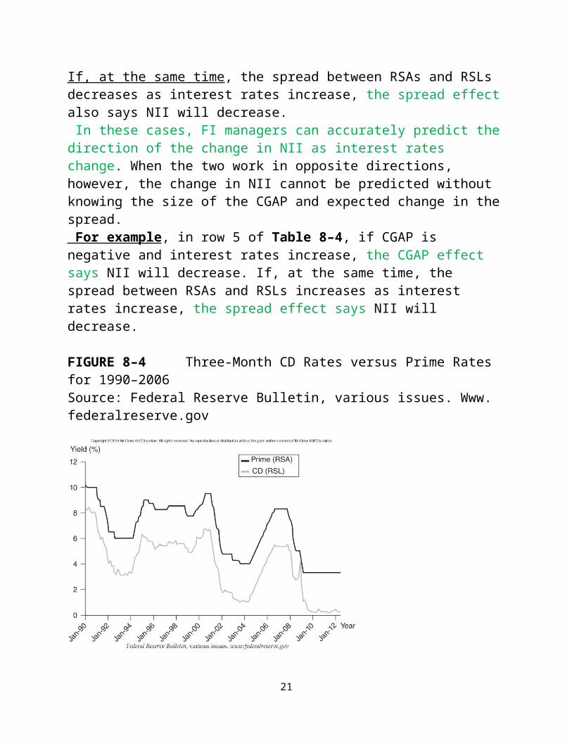
3.2 Unequal Changes in Rates on RSAs and RSLsThe previous section considered changes in net interest income as interest rates changed, assuming that the change in rates on RSAs was exactly equal to the change in rates on RSLs (in other words, assuming the interest rate spread between rates on RSAs and RSLs remained unchanged). This is not often the case; rather, rate changes on RSAs generally differ from those on RSLs (i.e., the spread between interest rates on assets and liabilities changes along with the levels of these rates). See Figure 8–4, which plots quarterly CD rates (liabilities) and prime lending rates (assets) for the period 1990–2006. Notice that although the rates generally move in the same direction, they are not perfectly correlated. In this case, as we consider the impact of rate changes on NII, we have a spread effect في التغير و األصول معدالت في التغير بين الفرق اثر

الخصوم .in addition to the CGAP effects معدالت

If the spread between the rate on RSAs and RSLs increases, when interest rates rise (fall), interest revenue increases (decreases) by more (less) than interest expense.

14

The result is an increase in NII. Conversely, if the spread between the rates on RSAs and RSLs decreases, when interest rates rise (fall), interest revenue increases (decreases) less (more) than interest expense, and NII decreases.

In general, the spread effect is such that, regardless of the direction of the change in interest rates, a positive relation occurs between changes in the spread (between rates on RSAs and RSLs) and changes in NII. Whenever the spread increases (decreases), NII increases (decreases).

Spread effect : The effect that a change in the spread between rates on RSAs and RSLs has on net interest income as interest rates change

EXAMPLE 8–2 Impact of Spread Effect on Net Interest Income

To understand spread effect, assume for a moment that RSAs equal RSLs equal $155 million.Suppose that rates rise by 1.2 percent on RSAs and by 1 percent on RSLs (i.e., the spread between the rates on RSAs and RSLs increases by 1.2 percent − 1 percent = 0.2 percent). The resulting change in NII is calculated as:

Δ NII = (RSA× Δ R RSA( - )RSL× Δ R RSL( = Δ Interest revenue -Δ Interest expense = ($155million × 1.2%) - ($155 million 1.0%) = $155million (1.2%) - 1.0%)$310,000 (2)See Table 8–4 for various combinations of CGAP and spread changes and their effects on NII. The first four rows in Table 8–4 consider an FI with a positive CGAP; the last four rows consider an FI with a negative CGAP.

15

Notice in Table 8–4 that both the CGAP and spread effects can have the same effect on NII. For example, in row 6 of Table 8–4, if CGAP is negative and interest rates increase, the CGAP effect says NII will decrease. If, at the same time, the spread between RSAs and RSLs decreases as interest rates increase, the spread effect also says NII will decrease. In these cases, FI managers can accurately predict the direction of the change in NII as interest rates change. When the two work in opposite directions, however, the change in NII cannot be predicted without knowing the size of the CGAP and expected change in the spread. For example, in row 5 of Table 8–4, if CGAP is negative and interest rates increase, the CGAP effect says NII will decrease. If, at the same time, the spread between RSAs and RSLs increases as interest rates increase, the spread effect says NII will decrease.

FIGURE 8–4 Three-Month CD Rates versus Prime Rates for 1990–2006Source: Federal Reserve Bulletin, various issues. Www. federalreserve.gov

Some FIs accept quite large interest rate exposures relative to their asset sizes. For example, the average one-year repricing gap ratio of Macatawa Bank Corporation (Grand Rapids, Michigan) was 5.23 percent at the end of 2005 (i.e.,it had considerably more

16

RSLs than RSAs). As interest rates rose from January through July 2006, Macatawa was exposed to significant net interest income losses due to the cost of refinancing its large amount of RSLs (relative to RSAs) at higher rates. Commercial banks have recently paid much closer attention to interest rate risk exposure, significantly reducing the gaps between RSAs and RSLs.نموذج The repricing gap خالصة

The repricing gap is the measure of interest rate risk historically used by FIs, and it is still the main measure of interest rate risk used by small community banks and thrifts.

In contrast to the market value–based models of interest rate risk discussed in the Appendix to this chapter and in Chapter 9, the repricing gap model is conceptually easy to understand and can easily be used to forecast changes in profitability for a given change in interest rates. The repricing gap can be used to allow an FI to structure its assets and liabilities or to go off the balance sheet to take advantage of a projected interest rate change. However, the repricing gap model has some major weaknesses that have resulted in regulators’ calling for the use of more comprehensive models (e.g. , the duration gap model) to measure interest rate risk. We next discuss some of the major weaknesses of the repricing model.

TABLE 8–4 Impact of CGAP on the Relation between Changes in Interest Rates and Changes in Net Interest Income, Allowing for Different Rate Changes for RSAs and RSLs.

Change in Change in Interest Rates spread NII Row CGAP 1 >0 ⇑⇑ ⇑ 2 >0 ⇑⇓⇑⇓ 3 >0 ⇓⇑⇑⇓ 4 >0 ⇓ ⇓ ⇓

17

5 <0 ⇑ ⇑⇑⇓ 6 <0 ⇑⇓⇓ 7 <0 ⇓⇑⇑ 8 <0 ⇓⇓ ⇑⇓4-WEAKNESSES OF THE REPRICING MODELDespite the fact that this model of interest rate risk is used by the vast majority of depository institutions in the United States, the repricing model has four major shortcomings: (1) It ignores market value effects of interest rate changes,(2) it is overaggregative, (3) it fails to deal with the problem of rate-insensitive asset and liability runoffs and prepayments, and (4) it ignores cash flows from off-balance-sheet activities.

In this section, we discuss each of these weaknesses in more detail.

4.1 Market Value EffectsAs was discussed in the overview of FI risks (Chapter 7), interest rate changes have a market value effect in addition to an income effect on asset and liability values.That is, the present value of the cash flows on assets and liabilities changes, in addition to the immediate interest received or paid on them, as interest rates change. In fact, the present values (and where relevant, the market prices) of virtually all assets and liabilities on an FI’s balance sheet change as interest rateschange. The repricing model ignores the market value effect—implicitly assuming a book value accounting approach. As such, the repricing gap is only a partial measure of the true interest rate exposure of an FI. As we discuss the market value–based measures of interest rate risk (below and in Chapter 9), we will highlight the impact that ignoring the market value effect has on the ability to accurately measure the overall interest rate risk of an FI.

18

4.2 OveraggregationThe problem of defining buckets over a range of maturities ignores information regarding the distribution of assets and liabilities within those buckets. For example The dollar values of RSAs and RSLs within any maturity bucket range may be equal; however, on average, liabilities may be repriced toward the end of the bucket’s range, while assets may be repriced toward the beginning, in which case a change in interest rates will have an effect on asset and liability cash flows thatwill not be accurately measured by the repricing gap approach.

Look at the simple example for the three-month to six-month bucket in Figure 8–5 . Note that $50 million more RSAs than RSLs are repriced between months 3 and 4, while $50 million more RSLs than RSAs are repriced between months 5 and 6. The bank in its call report would show a zero repricing gap for the three-month to six-month bucket [+50 + (-50) = 0]. But as you can easily see, the bank’s assets and liabilities are mismatched within the bucket. Clearly, the shorter the range over which bucket gaps are calculated, the smaller this problem is. If an FI manager calculated one-day bucket gaps out into the future, this would give a more accurate picture of the net interest income exposure to rate changes. Reportedly, many large banks have internal systems that indicate their repricing gaps on any given day in the future (252 days’ time, 1,329 days’ time, etc.). This suggests that although regulators require the reporting of repricing gaps over only relatively wide maturity bucket ranges, FI managers could set in place internal information systems to report the daily future patterns of such gaps.

4.3 The Problem of RunoffsIn the simple repricing model discussed above, we assumed that all consumer loans matured in 1 year or that all conventional mortgages matured in 30 years. In reality, the FI continuously originates and retires consumer and mortgage loans as it creates and retires deposits.

19

For example, today, some 30-year original maturity mortgages may have only 1 year left before they mature; that is, they are in their 29th year. In addition, these loans may be listed as 30-year mortgages (and included as not rate sensitive), yet they will sometimes be prepaid early as mortgage holders refinance their mortgages and/or sell their houses. Thus, the resulting proceeds will be reinvested at current market rates within the year. In addition, even if an asset or liability is rate insensitive, virtually all assets and liabilities (e.g., long-term mortgages) pay some principal and/or interest back to the FI in any given year.

As a result, the FI receives a runoff cash flow from its rate-insensitive portfolio that can be reinvested at current market rates; that is, this runoff cash flow component of a rate-insensitive asset or liability is itself rate sensitive. The FI manager can deal easily with this in the repricing model by identifying for each asset and liability item the estimated dollar cash flow that will run off within the next year and adding these amounts to the value of rate sensitive assets and liabilities.

Runoff: Periodic cash flow of interest and principal amortization payments on long-term assets, such as conventional mortgages, that can be reinvested at market rates.

FIGURE 8–5The Overaggregation Problem: The Three-Month to Six-Month Bucket

4.4 Cash Flows from Off-Balance-Sheet Activities

20

The RSAs and RSLs used in the repricing model generally include only the assets and liabilities listed on the balance sheet. Changes in interest rates will affect the cash flows on many off-balance-sheet instruments as well. For example, an FI might have hedged its interest rate risk with an interest rate futures contract (see Chapter 23). As interest rates change, these futures contracts—as part of the marking-to-market process—produce a daily cash flow (either positive or negative) for the FI that may offset any on-balance-sheet gap exposure. These offsetting cash flows from futures contracts are ignored by the simple repricing model and should (and could) be included in the model.

21