2012-01-1749

Experimental Analysis of Engine Exhaust Waste EnergyRecovery using Power Turbine Technology for Light Duty

ApplicationR. Dijkstra, D. Smeulders, M. Boot, R. Eichhorn

Eindhoven University of Technology, Netherlands

A. SerrarensDTI Automotive Mechatronics, Netherlands

J. LennbladVolvo Cars, Sweden

Copyright c© 2012 Society of Automotive Engineers, Inc.

ABSTRACT

An experimental analysis was executed on a NA (Nat-ural Aspirated) 4-stroke gasoline engine to investi-gate the potential of exhaust waste energy recoveryusing power turbine technology for light duty appli-cation. Restrictions with decreasing diameter weremounted in the exhaust to simulate different vane po-sitions of a VGT (Variable Geometry Turbine) and in-cylinder pressure measurements were performed toevaluate the effect of increased exhaust back pres-sure on intake- and exhaust pumping losses and onengine performance. Test points in the engine mapwere chosen on the basis of high residence time forthe vehicle during the NEDC (New European DrivingCycle). The theoretically retrievable power was cal-culated in case a turbine is mounted instead of a re-striction and the net balance was obtained betweenpumping power losses and recovered energy.

INTRODUCTION

Many solutions are related to increasing the efficiencyof the internal combustion engine (ICE) itself. How-ever, the technical limit for improvement of current en-gine designs is nearing and will not be sufficient tomeet future fuel economy targets without additionalmeasures. Other technologies are focused on trans-mission design or the recuperation of kinetic vehicleenergy such as several electric hybrid drive-trains.

Potentials for efficiency maximization of a running andbrake loaded engine is determined by all individual(in)efficiencies according to

ηb = ηcomb · ηtherm · ηGE · ηmech (1)

In this Equation ηcomb denotes the combustion effi-ciency, which is the fraction of the fuel energy sup-plied which is released in the combustion process.For equivalence ratios lower than one, the combus-tion efficiency is between 90 and 100 %. ηtherm de-notes the thermodynamic efficiency, which relates theactual work per cycle to the amount of fuel chemicalenergy released in the combustion process. Typicalvalues for the thermodynamic efficiency are nowa-days around 30 %. Furthermore, ηGE denotes thegas exchange efficiency and indicates how efficientthe gas moves through the different engine processcycle stages. Typical values for the gas exchange effi-ciency range from 50 up to 97 %, depending on load.Finally, ηmech is the mechanical efficiency, which isthe ratio of the brake (or useful) power delivered bythe engine to the net indicated power. Typical valuesvary from 0 to 90 % depending on engine speed andother parameters. By definition the mechanical effi-ciency is zero for 0 bar BMEP.

Further big improvements can only be obtained whenthe largest source of losses is addressed, namely ex-haust waste energy. This loss source can be ascribedto the poor thermodynamic efficiency. As a conse-quence, about 40 % of the ingoing fuel energy of to-day’s ICE’s is lost via the exhaust gas [1].

To recover some of these losses, different technolo-gies are under investigation in which the Rankine cy-cle and power turbine technology cover the largest

1

part. According to Ringler et al. [2], the recoverableamount of power in case of power turbine technologyis driven by pressure gradients and/or kinetic energywhile in case of the Rankine cycle a temperature dif-ference or exhaust heat is addressed. For this reasonthe Rankine cycle has a higher potential in terms ofheat utilization. However looking at complexity andcosts, power turbine technology can be a more at-tractive solution. Beside that, the use of power turbinetechnology does not exclude the use of other thermalprocesses.

While axial turbines are mainly used in heavy dutyand stationary applications because of their high ef-ficiency, radial turbines are mainly used for light dutyapplications. In contrast to the axial flow turbine, forwhich the efficiency decreases with size due to rel-atively large blade clearance effects, the radial flowturbine has the great advantage that it maintains arelatively high efficiency when reduced to small sizes.It can efficiently handle a high expansion ratio and isalso more robust and cheaper to manufacture thanan axial turbine. Furthermore it is able to accept quiteunfavorable unsteady inlet conditions like highly pul-sating flows, found in the exhaust of a ICE (InternalCombustion Engine), without a complete deteriorationof its performance [3].

In literature, several reports are presented on perfor-mance improvements or generated power with powerturbine technology driven by exhaust energy [4, 5, 6].However, in most of them the effect of increased ex-haust back pressure on engine performance is treatedvery briefly, only simulated, or not mentioned at all.

During earlier performed experiments [7], no signif-icant net improvement in specific fuel consumptionwas observed for overall system (engine with powerturbine) performance which is in contrast with resultsfrom Michon et al. [4]. The presumed cause was thatthe increased level of exhaust back pressure, com-pared to the natural aspirated case, increases the en-gine pumping losses. In a second experimental ses-sion performed by the authors, the effect of exhaustback pressure on pumping losses and engine perfor-mance was analyzed in more detail. This is very im-portant for further development of power turbine tech-nology for exhaust waste heat recovery purposes, butalso for any other technology that causes an increasein exhaust back pressure. The results from this anal-ysis are presented in this paper.

METHODOLOGY

The research goal is to quantitatively and qualitativelydetermine the effect of exhaust back pressure on en-

gine pumping losses and overall performance and toget insight into the theoretically maximum recoverableamount of power using power turbine technology.

Four engine operating points (see Table 1) were cho-sen on the basis of highest vehicle residence time ac-cording to the NEDC and for a significant amount ofexhaust mass flow.

Table 1: Engine Operating Points

EngineSpeed [rpm]

Engine Torque[Nm]

net IMEP[bar]

2300 20 1.92500 30 2.42750 50 3.42500 75 4.7

Restriction Hole Diameters [mm]45 35 25 20 15 12.5 11.25 10

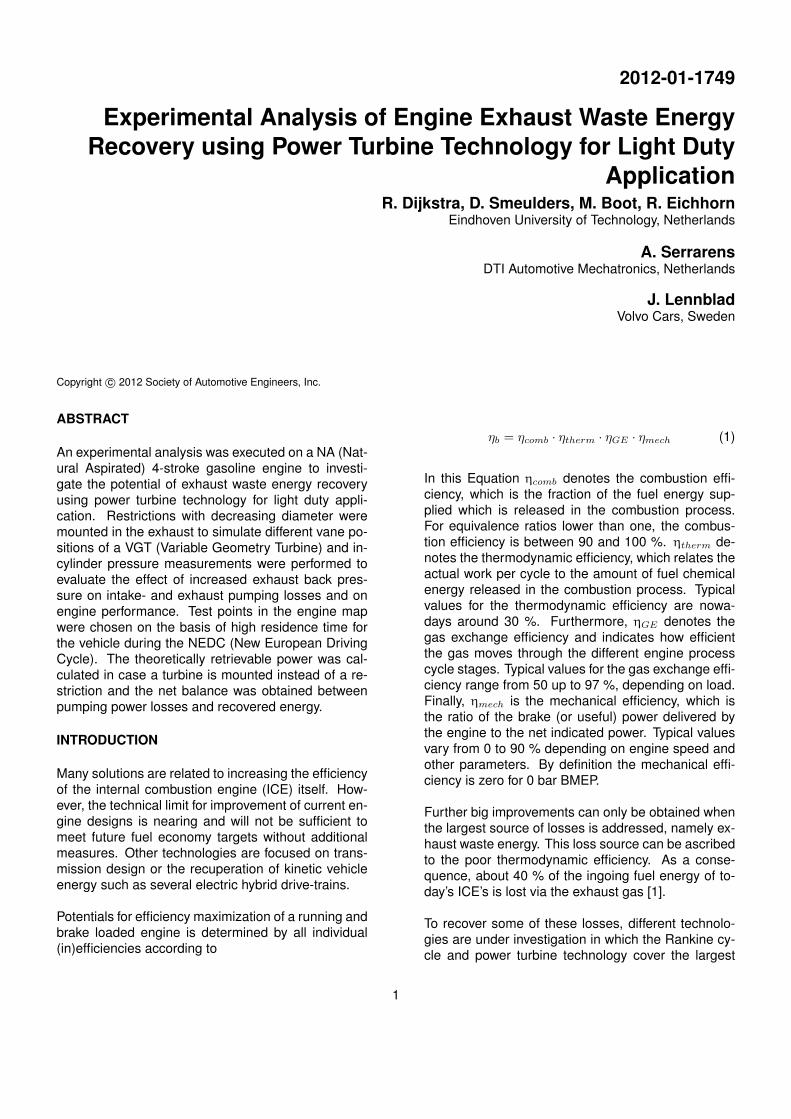
The engine residence map is depicted in Figure 1. Itis obtained by simulation of the NEDC with the specifi-cations of a Nissan SR20DE engine and a RS5F70Amanual transmission. The crosses denote the resi-dence of the engine. Higher vehicle residence is in-dicated by increasing square color strength and thechosen engine operating points are highlighted ingreen. Furthermore, relevant vehicle speeds are in-dicated in the map.

1000 1500 2000 2500 3000 3500

0

10

20

30

40

50

60

70

80

90

100

n [rpm]

T [N

m]

50 km/h

80 km/h

120 km/h

engine operating points

70 km/h

Figure 1: Chosen engine operating points highlightedin green in the engine residence map based on theresidence time according to the NEDC

To increase the exhaust back pressure eight orificeplate restrictions with decreasing hole diameter (seeTable 1) were mounted in the exhaust, where 45 mmis the exhaust diameter without restriction, and the in-cylinder pressure trace and other relevant parameterswere acquired. This was done for all four engine op-erating points. Instead of a back pressure valve, a

2

restriction was chosen for practical reasons and be-cause merely stationary points were analyzed.

EXPERIMENTAL SET-UP

For the experiments a Nissan 2 L four cylinder NA 4-stroke gasoline engine was used. The properties ofthe engine are listed in Table 2.

Table 2: Engine Properties

Bore [mm] 86Stroke [mm] 86Compression ratio 10Displacement [cm3] 1998Valve number 16Injection system PFI (Port Fuel Injection)

The in-cylinder pressure traces were acquired with a0.3 mm Kistler piezo quartz pressure transducer inte-grated in the spark plug which was mounted in onecylinder. Both crank-angle resolved and time aver-aged data were acquired during the measurements.The exhaust back pressure was measured in the ex-haust manifold, both crank-angle resolved and timeaveraged. Finally, the EGR (Exhaust Gas Recircula-tion) system of the engine was closed.

ANALYSIS

CRANK-ANGLE RESOLVED DATA

From the in-cylinder pressure trace, which wasmatched with intake pressure just before IVC (IntakeValve Closing), the aRoHR (apparent Rate of HeatRelease) was calculated with the assumption of anideal gas. Furthermore, net IMEP (Indicated MeanEffective Pressure) and PMEP (Pumping Mean Effec-tive Pressure) were calculated. The pumping losseswere individually calculated for the intake and exhauststroke.

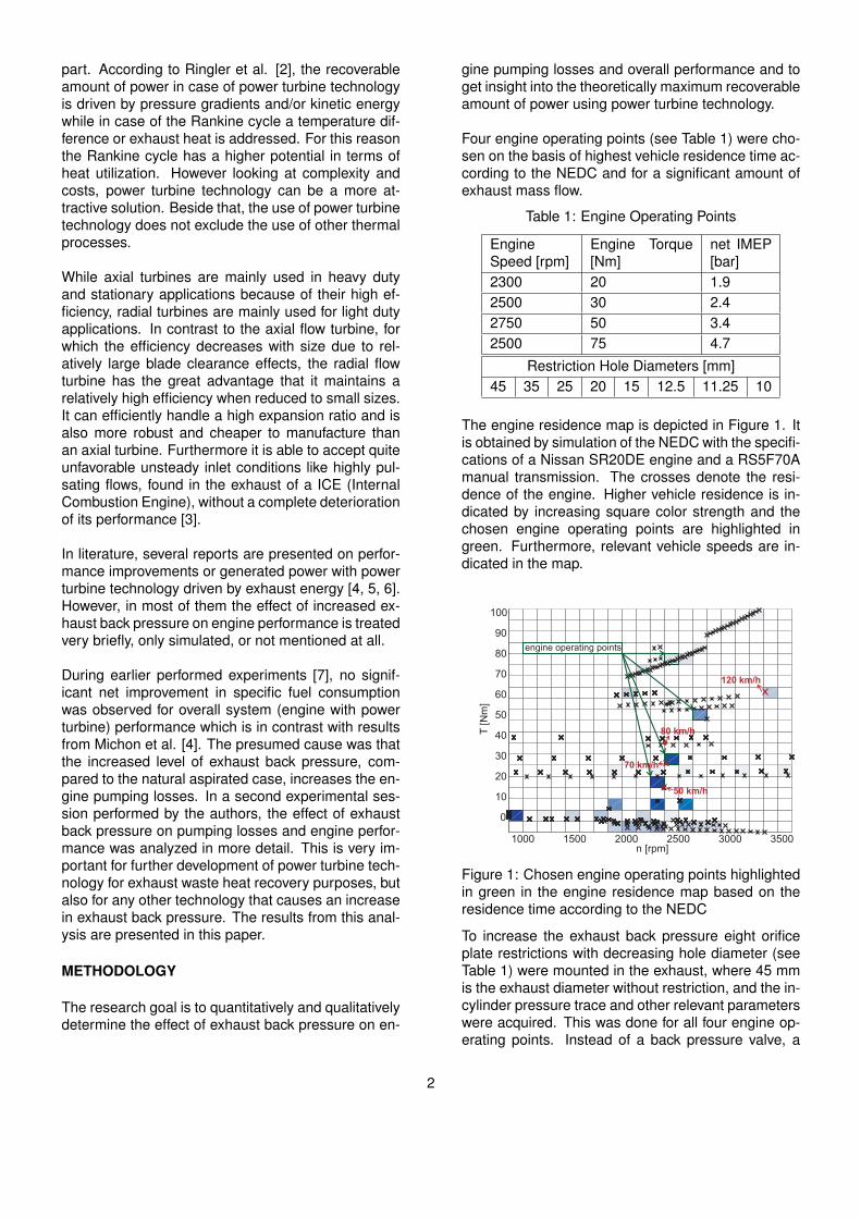
There are different conventions for the calculation ofthe pumping work. In this paper the 1:360o integra-tion convention is used, described by Shelby et al. [8],which includes area B plus area C in the total pump-ing losses (Figure 2).

This convention implicitly assumes that the work as-sociated with exchanging the exhaust gas with freshcharge occurs only during the exhaust and intakestrokes with no impact on the indicated work. Shelbyet al. proposed a new method to account for the in-accuracy introduced when valve timings deviate fromconventional timings (e.g. late intake valve closing),however for the engine described in this paper this is

V

p

TDC BDC

pch

pexh

A

B C

Figure 2: Pumping work in volume pressure diagram

not the case.

For NA engines the pumping work transfer is fromthe piston to the cylinder gases if the pressure dur-ing the intake stroke is less than the pressure duringthe exhaust stroke. For highly loaded turbo-chargedengines, the exhaust stroke pressure is usually lowerthan the intake pressure and therefore the pumpingwork transfer is from the cylinder gases to the piston.

a

bcd

e f g

( + V )Vc d

p

p

ch

atm

Vc V

p

Figure 3: Available energy turbine

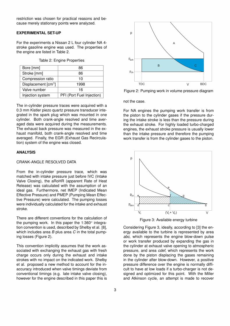
Considering Figure 3, ideally, according to [3] the en-ergy available to the turbine is represented by areaabc, which represents the engine blow-down pulseor work transfer produced by expanding the gas inthe cylinder at exhaust valve opening to atmosphericpressure, and area cdef, which represents the workdone by the piston displacing the gases remainingin the cylinder after blow-down. However, a positivepressure difference over the engine is normally diffi-cult to have at low loads if a turbo-charger is not de-signed and optimized for this point. With the Millerand Atkinson cycle, an attempt is made to recover

3

losses that are caused by the incomplete expansion(from point a to b). However, this comes at the costof engine power density. With the constant pressureprinciple a large exhaust manifold volume connectedto a turbine is used and the work represented by areabdeg is available to the turbine. With the pulse pres-sure principle on the other hand, where a small andshort exhaust manifold is used, an attempt is madeto utilize the work represented by both areas. Thisresults in a higher amount of energy available to theturbine for the pulse pressure principle.

TIME AVERAGED DATA

The available amount of power in the exhaust was cal-culated from the time averaged data using

Pav = mCpTexh

[(patmpexh

)κ−1κ

− 1

](2)

[3] which is valid for reversible isentropic expansion ofan ideal gas to atmospheric pressure. In the analysisthe kappa was calculated as function of temperature.

The ISFC (Indicated Specific Fuel Consumption) wascalculated from both crank-angle resolved and timeaveraged data.

RESULTS & DISCUSSION

PULSE OR CONSTANT PRESSURE

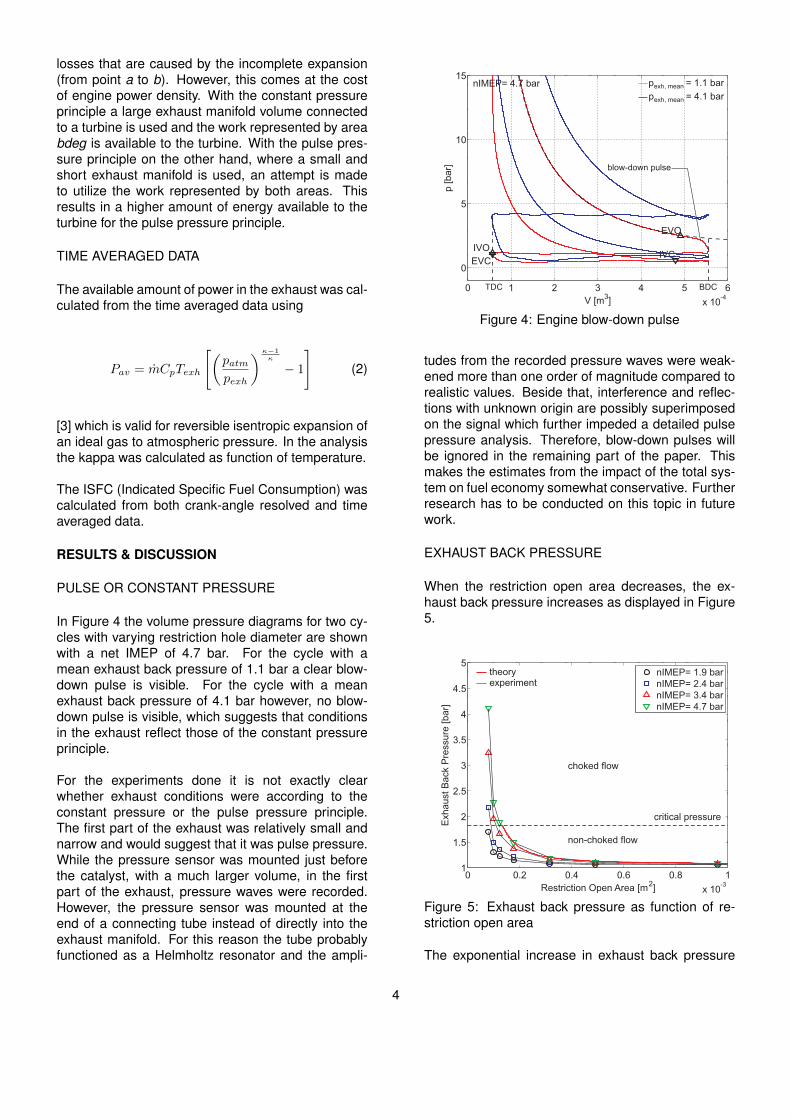
In Figure 4 the volume pressure diagrams for two cy-cles with varying restriction hole diameter are shownwith a net IMEP of 4.7 bar. For the cycle with amean exhaust back pressure of 1.1 bar a clear blow-down pulse is visible. For the cycle with a meanexhaust back pressure of 4.1 bar however, no blow-down pulse is visible, which suggests that conditionsin the exhaust reflect those of the constant pressureprinciple.

For the experiments done it is not exactly clearwhether exhaust conditions were according to theconstant pressure or the pulse pressure principle.The first part of the exhaust was relatively small andnarrow and would suggest that it was pulse pressure.While the pressure sensor was mounted just beforethe catalyst, with a much larger volume, in the firstpart of the exhaust, pressure waves were recorded.However, the pressure sensor was mounted at theend of a connecting tube instead of directly into theexhaust manifold. For this reason the tube probablyfunctioned as a Helmholtz resonator and the ampli-

0 1 2 3 4 5 6

x 10-4

0

5

10

15

V [m3]

p [b

ar]

EVCIVC

EVO

IVO

nIMEP= 4.7 bar

TDC BDC

blow-down pulse

p = 1.1 bar exh, mean

p = 4.1 bar exh, mean

Figure 4: Engine blow-down pulse

tudes from the recorded pressure waves were weak-ened more than one order of magnitude compared torealistic values. Beside that, interference and reflec-tions with unknown origin are possibly superimposedon the signal which further impeded a detailed pulsepressure analysis. Therefore, blow-down pulses willbe ignored in the remaining part of the paper. Thismakes the estimates from the impact of the total sys-tem on fuel economy somewhat conservative. Furtherresearch has to be conducted on this topic in futurework.

EXHAUST BACK PRESSURE

When the restriction open area decreases, the ex-haust back pressure increases as displayed in Figure5.

0 0.2 0.4 0.6 0.8 1

x 10-3

1

1.5

2

2.5

3

3.5

4

4.5

5

Restriction Open Area [m2]

Exh

au

st B

ack

Pre

ssu

re [b

ar]

nIMEP= 1.9 barnIMEP= 2.4 barnIMEP= 3.4 barnIMEP= 4.7 bar

critical pressure

choked flow

non-choked flow

theoryexperiment

Figure 5: Exhaust back pressure as function of re-striction open area

The exponential increase in exhaust back pressure

4

corresponds to the theory of a compressible flowthrough a flow restriction. The maximum mass flowoccurs when the velocity at the minimum area, orthroat, equals the velocity of sound. This is true when

p∗exh = patm ·(

2

κ+ 1

)κ/(κ−1)

(3)

[1] holds and the pressure for this to occur, p∗exh, is

called the critical exhaust back pressure. In this casethe exhaust gas flow becomes choked and the massflow is not able to increase any further. As a result,the maximum power of the engine decreases, withdecreasing restriction hole area, because higher loadimplies higher mass flow.

PUMPING WORK AND RECOVERABLE POWER

When the PMEP (Pumping Mean Effective Pressure)is evaluated for the different load cases (Figure 6) aclear linear trend is observed. When multiple regres-sion is applied to the data, a linear fit with a r-squaredof at least 99 % for all the load cases is found.

1 1.5 2 2.5 3 3.5 4 4.5−3.5

−3

−2.5

−2

−1.5

−1

−0.5

Exhaust Back Pressure [bar]

PM

EP

[bar

]

nIMEP= 1.9 barnIMEP= 2.4 barnIMEP= 3.4 barnIMEP= 4.7 bar

Figure 6: Pumping mean effective pressure as func-tion of exhaust back pressure

For low load, the initial PMEP is higher, which can beascribed to the higher pumping losses caused by thepartially closed throttle valve in the intake. The blackcrosses in Figure 6 denote the PMEP calculated from

PMEP = pint − pexh (4)

According to this equation, the PMEP is positive whenthe intake pressure is higher than the exhaust backpressure and vice versa.

In Figure 7 the exhaust PMEP is displayed for increas-ing exhaust back pressure. The trend for each load isvery similar and when multiple regression is applied alinear fit with a r-squared of nearly 100 % is found

PMEPexh = pexh − 1 (5)

The result from this relation is displayed by the blackcrosses.

1 1.5 2 2.5 3 3.5 4 4.50

0.5

1

1.5

2

2.5

3

3.5

4

Exhaust Back Pressure [bar]

PM

EP

exh [b

ar]

nIMEP= 1.9 barnIMEP= 2.4 barnIMEP= 3.4 barnIMEP= 4.7 bar

Figure 7: Exhaust pumping mean effective pressureas function of exhaust back pressure

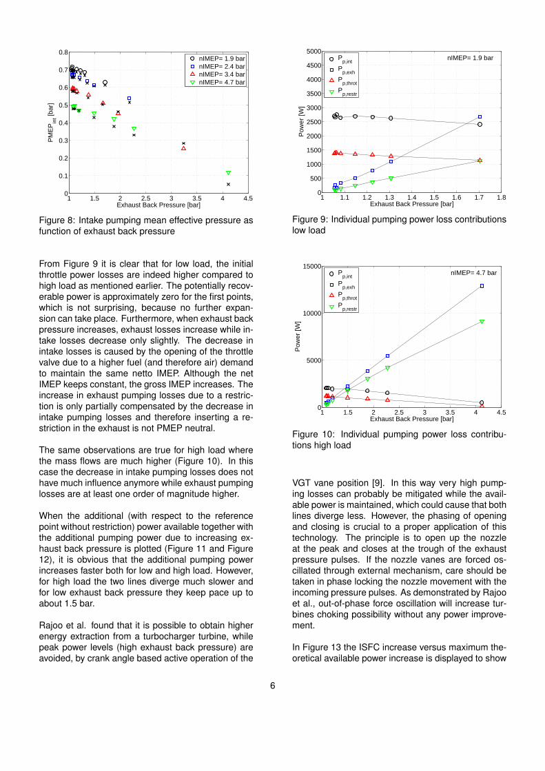
In Figure 8 the intake PMEP is displayed for increas-ing exhaust back pressure. Combining Equation 4and 5 yield

PMEPint = 1− pint (6)

The result from this Equation is displayed by the blackcrosses. Also for the intake PMEP a deviation is ob-served which increases with increasing exhaust backpressure. The initial intake PMEP decreases with in-creased engine load (nIMEP) and increasing exhaustback pressure, which is due to further opening of thethrottle valve. When the exhaust back pressure in-creases, the total pumping losses increase. To main-tain the same nIMEP the engine has to deliver morepower, which implicates further opening of the throttlevalve. This on its turn reduces the intake PMEP.

In Figure 9 and Figure 10 the individual pumpingpower loss contributions for intake (intake valve plusthrottle valve), exhaust (exhaust valve plus restric-tion), throttle valve and exhaust restriction are de-picted for low and high load respectively. The pump-ing power loss contribution for the restriction can alsobe interpreted as the potentially recoverable power(Equation 2).

5

1 1.5 2 2.5 3 3.5 4 4.50

0.1

0.2

0.3

0.4

0.5

0.6

0.7

0.8

Exhaust Back Pressure [bar]

PM

EP

int [b

ar]

nIMEP= 1.9 barnIMEP= 2.4 barnIMEP= 3.4 barnIMEP= 4.7 bar

Figure 8: Intake pumping mean effective pressure asfunction of exhaust back pressure

From Figure 9 it is clear that for low load, the initialthrottle power losses are indeed higher compared tohigh load as mentioned earlier. The potentially recov-erable power is approximately zero for the first points,which is not surprising, because no further expan-sion can take place. Furthermore, when exhaust backpressure increases, exhaust losses increase while in-take losses decrease only slightly. The decrease inintake losses is caused by the opening of the throttlevalve due to a higher fuel (and therefore air) demandto maintain the same netto IMEP. Although the netIMEP keeps constant, the gross IMEP increases. Theincrease in exhaust pumping losses due to a restric-tion is only partially compensated by the decrease inintake pumping losses and therefore inserting a re-striction in the exhaust is not PMEP neutral.

The same observations are true for high load wherethe mass flows are much higher (Figure 10). In thiscase the decrease in intake pumping losses does nothave much influence anymore while exhaust pumpinglosses are at least one order of magnitude higher.

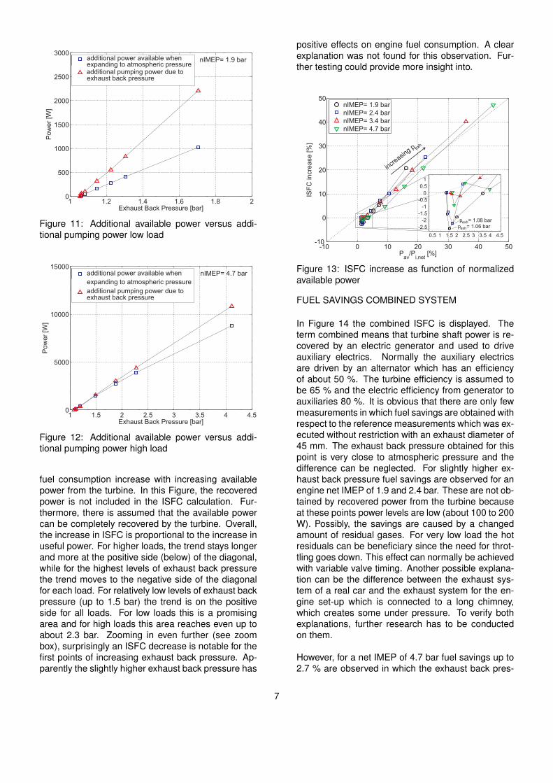
When the additional (with respect to the referencepoint without restriction) power available together withthe additional pumping power due to increasing ex-haust back pressure is plotted (Figure 11 and Figure12), it is obvious that the additional pumping powerincreases faster both for low and high load. However,for high load the two lines diverge much slower andfor low exhaust back pressure they keep pace up toabout 1.5 bar.

Rajoo et al. found that it is possible to obtain higherenergy extraction from a turbocharger turbine, whilepeak power levels (high exhaust back pressure) areavoided, by crank angle based active operation of the

1 1.1 1.2 1.3 1.4 1.5 1.6 1.7 1.80

500

1000

1500

2000

2500

3000

3500

4000

4500

5000

Exhaust Back Pressure [bar]

Pow

er [W

]

nIMEP= 1.9 barPp,int

Pp,exh

Pp,throt

Pp,restr

Figure 9: Individual pumping power loss contributionslow load

1 1.5 2 2.5 3 3.5 4 4.50

5000

10000

15000

Exhaust Back Pressure [bar]

Pow

er [W

]

nIMEP= 4.7 barPp,int

Pp,exh

Pp,throt

Pp,restr

Figure 10: Individual pumping power loss contribu-tions high load

VGT vane position [9]. In this way very high pump-ing losses can probably be mitigated while the avail-able power is maintained, which could cause that bothlines diverge less. However, the phasing of openingand closing is crucial to a proper application of thistechnology. The principle is to open up the nozzleat the peak and closes at the trough of the exhaustpressure pulses. If the nozzle vanes are forced os-cillated through external mechanism, care should betaken in phase locking the nozzle movement with theincoming pressure pulses. As demonstrated by Rajooet al., out-of-phase force oscillation will increase tur-bines choking possibility without any power improve-ment.

In Figure 13 the ISFC increase versus maximum the-oretical available power increase is displayed to show

6

1 1.2 1.4 1.6 1.8 20

500

1000

1500

2000

2500

3000

Exhaust Back Pressure [bar]

Po

we

r [W

]

nIMEP= 1.9 bar additional power available when

additional pumping power due toexpanding to atmospheric pressure

exhaust back pressure

Figure 11: Additional available power versus addi-tional pumping power low load

1 1.5 2 2.5 3 3.5 4 4.50

5000

10000

15000

Exhaust Back Pressure [bar]

Po

we

r [W

]

nIMEP= 4.7 baradditional power available when

additional pumping power due to

expanding to atmospheric pressure

exhaust back pressure

Figure 12: Additional available power versus addi-tional pumping power high load

fuel consumption increase with increasing availablepower from the turbine. In this Figure, the recoveredpower is not included in the ISFC calculation. Fur-thermore, there is assumed that the available powercan be completely recovered by the turbine. Overall,the increase in ISFC is proportional to the increase inuseful power. For higher loads, the trend stays longerand more at the positive side (below) of the diagonal,while for the highest levels of exhaust back pressurethe trend moves to the negative side of the diagonalfor each load. For relatively low levels of exhaust backpressure (up to 1.5 bar) the trend is on the positiveside for all loads. For low loads this is a promisingarea and for high loads this area reaches even up toabout 2.3 bar. Zooming in even further (see zoombox), surprisingly an ISFC decrease is notable for thefirst points of increasing exhaust back pressure. Ap-parently the slightly higher exhaust back pressure has

positive effects on engine fuel consumption. A clearexplanation was not found for this observation. Fur-ther testing could provide more insight into.

-10 0 10 20 30 40 50-10

0

10

20

30

40

50

Pav

/Pi,net

[%]

ISF

C in

cre

ase

[%

]

nIMEP= 1.9 barnIMEP= 2.4 barnIMEP= 3.4 barnIMEP= 4.7 bar

0.5 1 1.5 2 2.5 3 3.5 4 4.5

-2.5

-2

-1.5

-1

-0.5

0

0.5

1

increasin

g p xeh

p = 1.06 barexh

p = 1.08 barexh

Figure 13: ISFC increase as function of normalizedavailable power

FUEL SAVINGS COMBINED SYSTEM

In Figure 14 the combined ISFC is displayed. Theterm combined means that turbine shaft power is re-covered by an electric generator and used to driveauxiliary electrics. Normally the auxiliary electricsare driven by an alternator which has an efficiencyof about 50 %. The turbine efficiency is assumed tobe 65 % and the electric efficiency from generator toauxiliaries 80 %. It is obvious that there are only fewmeasurements in which fuel savings are obtained withrespect to the reference measurements which was ex-ecuted without restriction with an exhaust diameter of45 mm. The exhaust back pressure obtained for thispoint is very close to atmospheric pressure and thedifference can be neglected. For slightly higher ex-haust back pressure fuel savings are observed for anengine net IMEP of 1.9 and 2.4 bar. These are not ob-tained by recovered power from the turbine becauseat these points power levels are low (about 100 to 200W). Possibly, the savings are caused by a changedamount of residual gases. For very low load the hotresiduals can be beneficiary since the need for throt-tling goes down. This effect can normally be achievedwith variable valve timing. Another possible explana-tion can be the difference between the exhaust sys-tem of a real car and the exhaust system for the en-gine set-up which is connected to a long chimney,which creates some under pressure. To verify bothexplanations, further research has to be conductedon them.

However, for a net IMEP of 4.7 bar fuel savings up to2.7 % are observed in which the exhaust back pres-

7

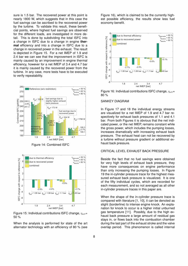
sure is 1.5 bar. The recovered power at this point isnearly 1800 W, which suggests that in this case thefuel savings can be ascribed to the recovered powerby the turbine. To validate this result, these benefi-cial points, where highest fuel savings are observedfor the different loads, are investigated in more de-tail. This is done by subdividing the total ISFC intoa change in ISFC due to a change in engine ther-mal efficiency and into a change in ISFC due to achange in recovered power in the exhaust. The resultis depicted in Figure 15. For a net IMEP of 1.9 and2.4 bar we can see that the improvement in ISFC ismainly caused by an improvement in engine thermalefficiency, however for a net IMEP of 3.4 and 4.7 barit is mainly caused by the recovered power from theturbine. In any case, more tests have to be executedto verify repeatability.

1.9 2.4 3.4 4.7180

190

200

210

220

230

240

250

260

270

280

Co

mb

ine

d IS

FC

[g

/kW

h]

halternator

= 50 %h

turbine= 65 %

helectric

= 80 %

Reference (w/o restriction)

net IMEP [bar]

248.3

241.3

-2.8%

217.4

223.2-2.6%

195.3

190.1-2.7%

206.7

204.9-0.9%

increasingexhaust back pressure

fuel savings due to slightly higher exhaust back pressure

fuel savings due to recovered power

P = 1798 Wrec

P = 173 Wrec

P = 109 Wrec

P = 334 Wrec

Figure 14: Combined ISFC

1.9 2.4 3.4 4.7-8

-6

-4

-2

0

2

4

6

8

ISF

C c

ha

ng

e w

ith r

esp

ect

to

re

fere

nce

[%

]

halternator

= 50 %h

turbine= 65 %

helectric

= 80 %

due to thermal efficiency

due to recovered power

combined

net IMEP [bar]

-2.8% -2.6%

-0.9%

-2.7%

p = 1.06 barexh

p = 1.08 barexh

p = 1.1 bar p = 1.49 barexh exh

Figure 15: Individual contributions ISFC change, ηalt=50 %

When the analysis is performed for state of the artalternator technology with an efficiency of 80 % (see

Figure 16), which is claimed to be the currently high-est possible efficiency, the results show less fueleconomy benefit.

1.8 2.4 3.4 4.7-8

-6

-4

-2

0

2

4

6

8

ISF

C c

ha

ng

e w

ith r

esp

ect to

re

fere

nce

[%

]

halternator

= 80 %h

turbine= 65 %

helectric

= 80 %

due to thermal efficiency

due to recovered power

combined

net IMEP [bar]

p = 1.06 barexh

p = 1.08 barexh

p = 1.1 bar p = 1.49 barexhexh

-2.7% -2.5%

-0.6%-0.1%

Figure 16: Individual contributions ISFC change, ηalt=80 %

SANKEY DIAGRAM

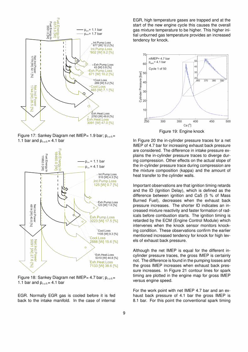
In Figure 17 and 18 the individual energy streamsare visualized for a net IMEP of 1.9 and 4.7 bar re-spectively for exhaust back pressures of 1.1 and 4.1bar. From both Figures it is obvious that the net indi-cated power, or the net IMEP, remains constant whilethe gross power, which includes the pumping losses,increases dramatically with increasing exhaust backpressure. The exhaust heat can not be recovered bya turbine without pressure gradient or additional ex-haust back pressure.

CRITICAL LEVEL EXHAUST BACK PRESSURE

Beside the fact that no fuel savings were obtainedfor very high levels of exhaust back pressure, theyhave more consequences on engine performancethan only increasing the pumping losses. In Figure19 the in-cylinder pressure trace for the highest mea-sured exhaust back pressure is visualized. It is oneof the fifty individual cycles, which are recorded foreach measurement, and so not averaged as all otherin-cylinder pressure traces in this paper are.

When the shape of the in-cylinder pressure trace iscompared with literature [1, 10], it can be denoted asslight (borderline) to intense engine knock. An expla-nation for knock to occur is a higher initial unburnedgas temperature [11]. Possibly, due to the high ex-haust back pressure a large amount of residual gasstays in, or flows back into the combustion chamberduring the last part of the exhaust stroke and the valveoverlap period. This phenomenon is called internal

8

Fu

el.E

ne

rgy.In

65

73

.0 [W

]

Int.Pump.Loss602 [W] 9.2 [%]

Exh.Pump.Loss671 [W] 10.2 [%]

Cool.Loss465 [W] 7.1 [%]

Exh.Heat.Loss3091 [W] 47.0 [%]

Ne

t.Ind

.Po

we

r1

74

4 [W

] 26

.5 [%

]

Fu

el.E

ne

rgy.In

55

51

.0 [W

]

Int.Pump.Loss677 [W] 12.2 [%]

Exh.Pump.Loss43 [W] 0.8 [%]

Cool.Loss289 [W] 5.2 [%]

Exh.Heat.Loss2763 [W] 49.8 [%]

Ne

t.Ind

.Po

we

r1

77

9 [W

] 32

.1 [%

]

p = 1.1 barexh

p = 1.7 barexh

Figure 17: Sankey Diagram net IMEP= 1.9 bar; pexh=1.1 bar and pexh= 4.1 bar

Fu

el.E

ne

rgy.In

118

62

.0 [W

]

Int.Pump.Loss510 [W] 4.3 [%]

Exh.Pump.Loss123 [W] 1.0 [%]

Cool.Loss1105 [W] 9.3 [%]

Exh.Heat.Loss5310 [W] 44.8 [%]

Ne

t.Ind

.Po

we

r4

81

4 [W

] 40

.6 [%

]

Fu

el.E

ne

rgy.In

18

46

0.0

[W]

Int.Pump.Loss125 [W] 0.7 [%]

Exh.Pump.Loss3223 [W] 17.5 [%]

Cool.Loss2888 [W] 15.6 [%]

Exh.Heat.Loss7133 [W] 38.6 [%]

Ne

t.Ind

.Po

we

r5

09

1 [W

] 27

.6 [%

]

p = 4.1 barexh

p = 1.1 barexh

Figure 18: Sankey Diagram net IMEP= 4.7 bar; pexh=1.1 bar and pexh= 4.1 bar

EGR. Normally EGR gas is cooled before it is fedback to the intake manifold. In the case of internal

EGR, high temperature gases are trapped and at thestart of the new engine cycle this causes the overallgas mixture temperature to be higher. This higher ini-tial unburned gas temperature provides an increasedtendency for knock.

250 300 350 400 450 5000

10

20

30

40

50

60

70

Ca [o]

Cyl

ind

er

Pre

ssu

re [b

ar]

360 370 380 39025

35

45

55nIMEP= 4.7 barp = 4.1 bar

Cycle 1 of 50

exh

Figure 19: Engine knock

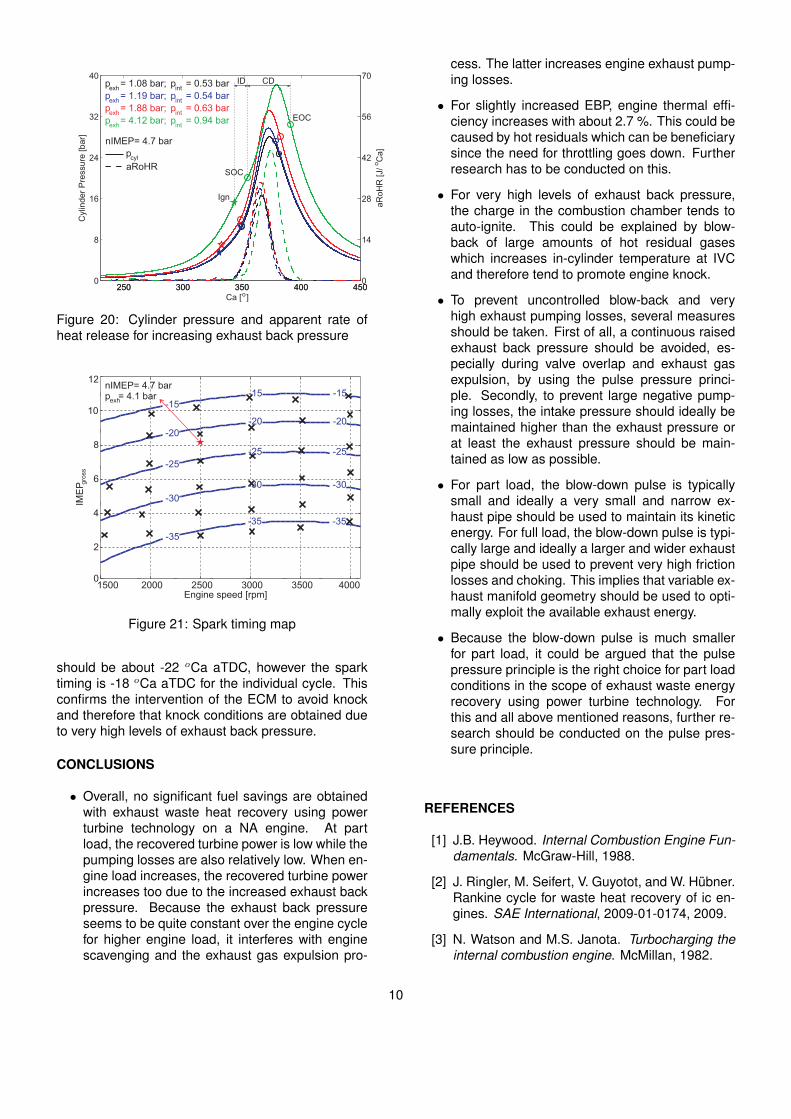
In Figure 20 the in-cylinder pressure traces for a netIMEP of 4.7 bar for increasing exhaust back pressureare considered. The difference in intake pressure ex-plains the in-cylinder pressure traces to diverge dur-ing compression. Other effects on the actual slope ofthe in-cylinder pressure trace during compression arethe mixture composition (kappa) and the amount ofheat transfer to the cylinder walls.

Important observations are that ignition timing retardsand the ID (Ignition Delay), which is defined as thedifference between ignition and Ca5 (5 % of MassBurned Fuel), decreases when the exhaust backpressure increases. The shorter ID indicates an in-creased mixture reactivity and faster formation of rad-icals before combustion starts. The ignition timing isretarded by the ECM (Engine Control Module) whichintervenes when the knock sensor monitors knock-ing condition. These observations confirm the earliermentioned increased tendency for knock for high lev-els of exhaust back pressure.

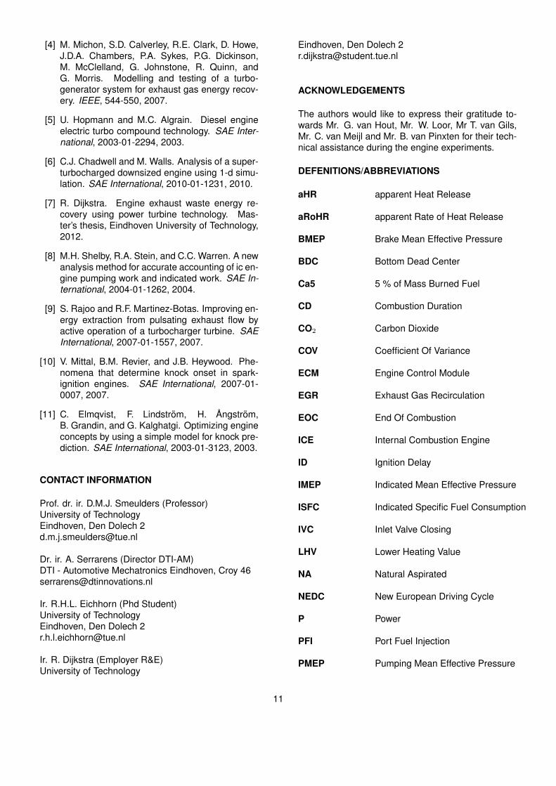
Although the net IMEP is equal for the different in-cylinder pressure traces, the gross IMEP is certainlynot. The difference is found in the pumping losses andthe gross IMEP increases when exhaust back pres-sure increases. In Figure 21 contour lines for sparktiming are plotted in the engine map for gross IMEPversus engine speed.

For the work point with net IMEP 4.7 bar and an ex-haust back pressure of 4.1 bar the gross IMEP is8.1 bar. For this point the conventional spark timing

9

250 300 350 400 4500

8

16

24

32

40C

ylin

de

r P

ress

ure

[b

ar]

oCa [ ]

Ign

SOC

EOC

ID

250 300 350 400 4500

14

28

42

56

70

aR

oH

R [J/

oC

a]

pint

= 0.53 bar

pint

= 0.54 bar

pint

= 0.63 bar

intp = 0.94 bar

pexh

= 1.08 bar;

pexh

= 1.19 bar;

pexh

= 1.88 bar;

exhp = 4.12 bar;

nIMEP= 4.7 bar

pcyl

aRoHR

CD

Figure 20: Cylinder pressure and apparent rate ofheat release for increasing exhaust back pressure

1500 2000 2500 3000 3500 40000

2

4

6

8

10

12

-35

-35

-30

-30

-25

-25

-20-20

-15-15

Engine speed [rpm]

IME

P gro

ss

-35

-30

-25

-20

-15nIMEP= 4.7 barp = 4.1 bar

exh

Figure 21: Spark timing map

should be about -22 oCa aTDC, however the sparktiming is -18 oCa aTDC for the individual cycle. Thisconfirms the intervention of the ECM to avoid knockand therefore that knock conditions are obtained dueto very high levels of exhaust back pressure.

CONCLUSIONS

• Overall, no significant fuel savings are obtainedwith exhaust waste heat recovery using powerturbine technology on a NA engine. At partload, the recovered turbine power is low while thepumping losses are also relatively low. When en-gine load increases, the recovered turbine powerincreases too due to the increased exhaust backpressure. Because the exhaust back pressureseems to be quite constant over the engine cyclefor higher engine load, it interferes with enginescavenging and the exhaust gas expulsion pro-

cess. The latter increases engine exhaust pump-ing losses.

• For slightly increased EBP, engine thermal effi-ciency increases with about 2.7 %. This could becaused by hot residuals which can be beneficiarysince the need for throttling goes down. Furtherresearch has to be conducted on this.

• For very high levels of exhaust back pressure,the charge in the combustion chamber tends toauto-ignite. This could be explained by blow-back of large amounts of hot residual gaseswhich increases in-cylinder temperature at IVCand therefore tend to promote engine knock.

• To prevent uncontrolled blow-back and veryhigh exhaust pumping losses, several measuresshould be taken. First of all, a continuous raisedexhaust back pressure should be avoided, es-pecially during valve overlap and exhaust gasexpulsion, by using the pulse pressure princi-ple. Secondly, to prevent large negative pump-ing losses, the intake pressure should ideally bemaintained higher than the exhaust pressure orat least the exhaust pressure should be main-tained as low as possible.

• For part load, the blow-down pulse is typicallysmall and ideally a very small and narrow ex-haust pipe should be used to maintain its kineticenergy. For full load, the blow-down pulse is typi-cally large and ideally a larger and wider exhaustpipe should be used to prevent very high frictionlosses and choking. This implies that variable ex-haust manifold geometry should be used to opti-mally exploit the available exhaust energy.

• Because the blow-down pulse is much smallerfor part load, it could be argued that the pulsepressure principle is the right choice for part loadconditions in the scope of exhaust waste energyrecovery using power turbine technology. Forthis and all above mentioned reasons, further re-search should be conducted on the pulse pres-sure principle.

REFERENCES

[1] J.B. Heywood. Internal Combustion Engine Fun-damentals. McGraw-Hill, 1988.

[2] J. Ringler, M. Seifert, V. Guyotot, and W. Hubner.Rankine cycle for waste heat recovery of ic en-gines. SAE International, 2009-01-0174, 2009.

[3] N. Watson and M.S. Janota. Turbocharging theinternal combustion engine. McMillan, 1982.

10

[4] M. Michon, S.D. Calverley, R.E. Clark, D. Howe,J.D.A. Chambers, P.A. Sykes, P.G. Dickinson,M. McClelland, G. Johnstone, R. Quinn, andG. Morris. Modelling and testing of a turbo-generator system for exhaust gas energy recov-ery. IEEE, 544-550, 2007.

[5] U. Hopmann and M.C. Algrain. Diesel engineelectric turbo compound technology. SAE Inter-national, 2003-01-2294, 2003.

[6] C.J. Chadwell and M. Walls. Analysis of a super-turbocharged downsized engine using 1-d simu-lation. SAE International, 2010-01-1231, 2010.

[7] R. Dijkstra. Engine exhaust waste energy re-covery using power turbine technology. Mas-ter’s thesis, Eindhoven University of Technology,2012.

[8] M.H. Shelby, R.A. Stein, and C.C. Warren. A newanalysis method for accurate accounting of ic en-gine pumping work and indicated work. SAE In-ternational, 2004-01-1262, 2004.

[9] S. Rajoo and R.F. Martinez-Botas. Improving en-ergy extraction from pulsating exhaust flow byactive operation of a turbocharger turbine. SAEInternational, 2007-01-1557, 2007.

[10] V. Mittal, B.M. Revier, and J.B. Heywood. Phe-nomena that determine knock onset in spark-ignition engines. SAE International, 2007-01-0007, 2007.

[11] C. Elmqvist, F. Lindstrom, H. Angstrom,B. Grandin, and G. Kalghatgi. Optimizing engineconcepts by using a simple model for knock pre-diction. SAE International, 2003-01-3123, 2003.

CONTACT INFORMATION

Prof. dr. ir. D.M.J. Smeulders (Professor)University of TechnologyEindhoven, Den Dolech 2d.m.j.smeulders@tue.nl

Dr. ir. A. Serrarens (Director DTI-AM)DTI - Automotive Mechatronics Eindhoven, Croy 46serrarens@dtinnovations.nl

Ir. R.H.L. Eichhorn (Phd Student)University of TechnologyEindhoven, Den Dolech 2r.h.l.eichhorn@tue.nl

Ir. R. Dijkstra (Employer R&E)University of Technology

Eindhoven, Den Dolech 2r.dijkstra@student.tue.nl

ACKNOWLEDGEMENTS

The authors would like to express their gratitude to-wards Mr. G. van Hout, Mr. W. Loor, Mr T. van Gils,Mr. C. van Meijl and Mr. B. van Pinxten for their tech-nical assistance during the engine experiments.

DEFENITIONS/ABBREVIATIONS

aHR apparent Heat Release

aRoHR apparent Rate of Heat Release

BMEP Brake Mean Effective Pressure

BDC Bottom Dead Center

Ca5 5 % of Mass Burned Fuel

CD Combustion Duration

CO2 Carbon Dioxide

COV Coefficient Of Variance

ECM Engine Control Module

EGR Exhaust Gas Recirculation

EOC End Of Combustion

ICE Internal Combustion Engine

ID Ignition Delay

IMEP Indicated Mean Effective Pressure

ISFC Indicated Specific Fuel Consumption

IVC Inlet Valve Closing

LHV Lower Heating Value

NA Natural Aspirated

NEDC New European Driving Cycle

P Power

PFI Port Fuel Injection

PMEP Pumping Mean Effective Pressure

11

Q Thermal Energy

SOC Start Of Combustion

ST Spark Timing

TDC Top Dead Center

V Volume

VGT Variable Geometry Turbine

W Work

WOT Wide Open Throttle

atm atmospheric

alt alternator

av available

b brake

cc crankcase

ch charging

comb combustion

conv conventional

cyl cylinder

d displacement

elec electric

exh exhaust

f fuel

fric friction

GE gas exchange

i indicated

mech mechanical

p pumping

rec recovered

therm thermodynamic

tot total

tur turbine

ISFC = 3.6× 106 · mf

Pi,net

ISFCnew = 3.6× 106 · mf

Pi,net + Pav · ηtur · ηelec · 1ηalt

IMEPnet =Wi,net

Vd

PMEP =Wp,tot

Vd

Wp,tot =Wp,int + |Wp,exh|

Wp,int =

∫ 180

oCa=0

(pcc − pcyl)∂V

∂αdα

Wp,exh =

∫ 720

oCa=540

(pcyl − pcc)∂V

∂αdα

ηcomb =HR (TA)−HP (TA)

mfQHV,f

ηtherm =Pi,gross

ηcmfQHV,f

ηGE =Pi,netPi,gross

= 1− PpPi,gross

ηmech =Pb

Pi,net= 1− Pfric

Pi,net

ηf = ηcomb · ηtherm

ηi,net = ηcomb · ηtherm · ηGE

ηb = ηcomb · ηtherm · ηGE · ηmech

12