Expected Returns and Volatility of Fama-French Factors

Fousseni CHABI-YO∗

Fisher College of Business, Ohio State University

First Version August 15, 2009. This Version September 25, 2009

Abstract

In this paper, I show that the variance of Fama-French factors, the variance of the momentum

factor, as well as the correlation between these factors, predict an important fraction of the time-

series variation in post-1990 aggregate stock market returns. This predictability is particularly

strong from one month to one year, and it dominates that afforded by the variance risk premium

and other popular predictor variables such as P/D ratio, the P/E ratio, the default spread,

and the consumption-wealth ratio. In a simple representative agent economy with recursive

preferences, I model the portfolio weight in each asset as a function of a stock’s characteristics

and show that the market return can be predicted by these variances.

(JEL C22, C51, C52, G12, G13, G14)

∗Fousseni CHABI-YO is from the Fisher College of Business, The Ohio State University. I am grateful to KeweiHou, Rene Stulz, Hao Zhou, Ingrid Werner, and seminar participants at the Ohio State University. I thank KennethFrench for making a large amount of historical data publicly available in his online data library. I welcome comments,including references to related papers I have inadvertently overlooked. I thank the Dice Center for Financial Economicsfor financial support. Correspondence Address: Fousseni Chabi-Yo, Fisher College of Business, Ohio State University,840 Fisher Hall, 2100 Neil Avenue, Columbus, OH 43210-1144. email: chabi-yo 1@fisher.osu.edu

Expected Returns and Volatility of Fama-French Factors

Abstract

In this paper, I show that the variance of Fama-French factors, the variance of the momentum

factor, as well as the correlation between these factors, predict an important fraction of the time-

series variation in post-1990 aggregate stock market returns. This predictability is particularly

strong from one month to one year, and it dominates that afforded by the variance risk premium

and other popular predictor variables such as P/D ratio, the P/E ratio, the default spread,

and the consumption-wealth ratio. In a simple representative agent economy with recursive

preferences, I model the portfolio weight in each asset as a function of a stock’s characteristics

and show that the market return can be predicted by these variances.

(JEL C22, C51, C52, G12, G13, G14)

I. Introduction

Recently, Bollerslev et al. (2009) and Zhou (2009) show that the difference between “model-free”

implied and realized variances, which they term the variance risk premium, predicts an important

fraction of the variation in post-1990 aggregate stock market returns with high (low) values of the

premium associated with subsequent high (low) returns. They show that the magnitude of the

predictability is particularly strong at the intermediate three months return horizon, in which it

dominates that afforded by other popular predictor variables, such as the P/E ratio, the default

spread, and the consumption–wealth ratio. It seems that the predictability of the variance risk

premium is the strongest at a short horizon but the predictability of variables such as P/E ratio,

the default spread, and the consumption–wealth ratio is strongest at the medium and long horizons.

The variance risk premium has been interpreted as an indicator of the representative agent’s risk

aversion. Recent papers rely on the non-standard recursive utility framework of Epstein and Zin

(1991) and Weil (1989) to show that the variance risk premium is due to the macroeconomic

uncertainty risk.

I utilize stock’s characteristics such as the firm’s market capitalization, book-to-market ratio,

or lagged return to study the predictability of market returns. In a simple representative agent

economy with recursive preferences, I allow the portfolio weights to be a function of the asset’s

characteristics, as in Brandt et al. (2009), and show that the market return can be predicted

by the variance of the Fama and French factors: size (SMB), book-to-market factor (HML); the

variance of the momentum factor (MOM), as well as the correlation between these factors. Asset’s

characteristics, such as the firm’s market capitalization, book-to-market ratio, or lagged return, are

related to the stocks expected return. Fama and French (1996) find that these three characteristics

robustly describe the cross-section of expected returns1.

I use S&P500 returns to compute the holding period returns from January 1990 to December

2008, and look first at the predictability of the aforementioned variables. The degree of predictabil-

ity offered by the HML variance starts out fairly high at the monthly horizon with an adjusted R2

of 4.94%. The robust t-statistic for testing the estimated slope coefficient associated with the HML

variance is -2.78. The three-month return regression results in a much more impressive t-statistic1Chan, Karceski, and Lakonishok (1998) show that these characteristics are also related to the variances and

covariances of returns. Lewellen (2004), Ang and Bekaert (2007), Campbell and Yogo (2006) provide extensivediscussion about return predictability.

3

of -3.59 with a corresponding adjusted R2 of 9.69%. The adjusted R2 remains high and ranges

from 9% to 13% from six-month to two-year horizon. The t-statistic also remains highly signifi-

cant and ranges from -5.02 to -3.52 for all horizons. Also noteworthy is that the monthly HML

variance series is less correlated with the variance risk premium. The correlation of the monthly

HML variance series with the variance risk premium is 0.07 for the 1990-2007 period, and -0.18 for

the 1990-2008 period. The degree of predictability offered by the HML variance dominates that

afforded by the variance risk premium. With the variance risk premium, the adjusted R2 starts out

at the monthly horizon at 3.24%. The robust t-statistic for testing the estimated slope coefficient

associated with the variance risk premium is 4.47. The three-month return regression also results

in an impressive t-statistic of 3.30 with a corresponding R2 of 6.02%, but the numerical values and

significance gradually taper off for longer return horizons.

The degree of predictability offered by the MOM variance starts out fairly high at the monthly

horizon with an adjusted R2 of 3.61%. The quarterly return regression results in a much more

impressive R2 of 11.40%. The adjusted R2 remains high at six-month horizon (14.84%) and ranges

from 14% to 15% from nine-month horizon to eighteen-month horizon, then decreases to 11.18%

at the two-year horizon. The t-statistic also remains highly significant and ranges from -4.51 to

-3.25 for all horizons. Although the degree of predictability of the MOM variance series exceeds

the degree of predictability offered by the variance risk premium, it is important to point out

that the MOM variance series is less correlated with the variance risk premium. The correlation

of the monthly MOM variance series with the variance risk premium is -0.07 for the 1990-2007

period, and -0.14 for the 1990-2008 period. Also noteworthy is that, at monthly and quarterly

horizons, the degree of predictability offered by the HML or MOM variance dominates that afforded

by other popular predictor variables, such as the P/D ratio, P/E ratio, the default spread, and

the consumption−wealth ratio (CAY). Surprisingly, taken alone, the monthly SMB variance series

cannot predict the S&P500 at all horizons. The degree of predictability offered by the SMB variance

is low at 1.6% at the one-month horizon and 2.12% at the two-year horizon.

The correlation series between the market and the HML factor is less correlated with the variance

risk premium series (-0.34). The degree of predictability afforded by this correlation measure is

similar but slightly higher than that afforded by the variance risk premium at all horizons, except

the one-month horizon. The adjusted R2 is 5.09% at the three-month horizon, then peaks around

4

the six-month horizon at 10.65%, and the nine-month horizon at 10.12%, then gradually tapers

off at longer return horizons. The degree of predictability afforded by the correlation between the

market and the SMB factor starts high at 6.12% at nine-month horizon, then gradually increases

for longer return horizons. The degree of predictability afforded by the correlation between the

HML and the SMB factors starts fairly high at 4.42% at the six-month horizon, then gradually

increases for longer return horizons. The other correlation measures have a negligible impact on

the S&P500 returns.

Second, I look at the predictability afforded by a combination of these variables. I use a

combination of the HML and MOM variance series, the correlation between series between the

market return and the Fama-French factors, and the correlation between the market return and

momentum factor. This combination predicts an important fraction of the variation in post-1990

aggregate stock market returns. The magnitude of the predictability is particularly strong and

dominates that afforded by other popular predictor variables. The degree of predictability offered

by this combination starts at 8.85% at the monthly horizon, then increases to 20.96% at the three-

month horizon, reaches 24.79% at the semi-annual return horizon, and 29.19% at the nine-month

horizon. Combining the variance risk premium with the HML and MOM variance series as well as

the monthly correlation series results in even greater return predictability and joint significance of

the predictor variables. The adjusted R2 starts at 10.07% at the one-month horizon, then increases

to 22.51% at three-month horizon, reaches 26% at semi-annual return horizon, and peaks at 29.45%

at the nine-month return horizon. Combining the aforementioned predictor variables, the variance

premium, and some of standard predictor variables results in an impressive adjusted R2.

My model may be seen as an extension of the variance risk premium model pioneered by Boller-

slev et al. (2009) who emphasized the importance of variance risk premium for predicting the S&P

500 returns over short horizons. In contrast to Bollerslev et al. (2009), I allow the portfolio weights

to depend on stock characteristics. This allows me to generate a testable model to investigate the

degree of predictability afforded by the HML and MOM variances, and aforementioned correlation

measures.

The plan for the rest of the paper is as follows. Section II outlines the theoretical model

and corresponding predictability regressions that motivate my empirical investigations. Section III

discusses the data that I use in empirically quantifying the predictor variables. Section IV presents

5

my main empirical findings and robustness checks. Section V concludes.

II. Volatility Risk and Predictability of Returns

I consider an economy with a representative agent who is equipped with Epstein–Zin–Weil recursive

preferences. The representative household maximizes recursive utility over consumption following

Kreps and Porteus (1978), Epstein and Zin (1989), and Weil (1989):

Ut ={

(1− β) Cρt + β

(Et

[Uα

t+1

])ρ/α} 1

ρ (1)

where Ct denotes consumption and β ∈ (0, 1). Here, ρ < 1 captures time preference (the Elasticity

of Intertemporal Substitution (EIS) is 1/ (1− ρ)). The EIS measures the agents willingness to

postpone consumption overtime, a notion well-defined even under certainty. the α < 1 captures

risk aversion (the coefficient of relative risk aversion is 1− α). Relative risk aversion measures the

agents aversion to atemporal risk across states. The innovation relative to additive utility is that

ρ and α need not be equal. I refer to these preferences, as Kreps and Porteus do, to distinguish

them from other preferences described by Epstein and Zin. We know from Epstein and Zin that

the Euler equation for any return Rit+1 can be stated as

Et [Mt+1Ri,t+1] = 1,

with

Mt+1 = βγ

(Ct+1

Ct

)(ρ−1)γ

Rγ−1p,t+1. (2)

where γ = αρ , and Rp,t+1 is the gross return on the optimal portfolio. The logarithm of the pricing

kernel (2) may be expressed as

mt+1 = γ log β + (ρ− 1) γgt+1 + (γ − 1) rp,t+1,

where

rpt+1 = ωᵀt rt+1

is the representative agent’s optimal portfolio return, rt+1 represents the vector of return on the

risky assets, ωt = {ωit}i=1,...N represents the optimal portfolio weight in this economy, and gt+1

is the log consumption growth rate. I closely follow Brandt et al. (2009) and parameterize the

optimal portfolio weights as a function of the stock’s characteristics xit;

ωit = f (xit; φ) . (3)

6

I use the following simple linear specification for the portfolio weight function:

ωit = ωit +1Nt

φᵀx̂it, (4)

where ωit is the weight of stock i at date t in a benchmark portfolio, such as the value-weighted

market portfolio; φ is a vector of coefficients; and x̂it are the characteristics of stock i , standardized

cross-sectionally to have zero mean and unit standard deviation across all stocks at date t. As

shown in Brandt et al. (2009), the linear policy (4) conveniently nests the long–short portfolio

constructions of Fama and French (1993) or their extension in Carhart (1997). To understand how

this is the case, assume that the portfolio policy in equation (3) is parameterized in a linear manner

as in (4). Let the benchmark weights be the market capitalization weights and the characteristics

are defined as 1 if the stock is in a top quantile; −1 if it is in the bottom quantile; and 0 for

intermediate quantiles of market capitalization (me), book to market ratio (btm), and the past

return (mom). Then, the optimal portfolio return is

rpt+1 = rMt+1 + φmerSMBt+1 + φbtmrHMLt+1 + φmomrMOMt+1 (5)

with

rMt+1 =Nt∑

i=1

ωitrit+1, (6)

and

rSMBt+1 =Nt∑

i=1

(1Qt

mei,t

)rit+1, (7)

rHMLt+1 =Nt∑

i=1

(1Qt

btmi,t

)rit+1, (8)

rMOMt+1 =Nt∑

i=1

(1Qt

momi,t

)rit+1, (9)

where rSMBt+1, rHMLt+1, and rMOMt+1 are the returns of “small-minus-big”(SMB), “high-minus-

low,”(HML) and “winners-minus-losers ”(MOM) portfolios, and Qt is the number of firms in the

quantile. The phi coefficients are the weights put on each of the factor portfolios. The expected

excess return on the optimal portfolio is

Etrpt+1 − rf = −covt (mt+1, rpt+1) . (10)

7

Now, I closely follow Bollerslev et al. (2009) and suppose that the geometric growth rate of

consumption in the economy is not predictable. In addition, I assume that the volatility of the

consumption growth follows a stochastic process

gt+1 = µgt + σgtzgt+1, (11)

σ2gt+1 = aσ + ρgσ

2gt +

√qtzσt+1, (12)

qt+1 = aq + ρqqt + ϕq√

qtzqt+1, (13)

where aσ > 0 , aq > 0, |ρg| < 1, |ρq| < 1 and ϕq > 0. The parameter µgt denotes the constant mean

growth rate, σgt is the conditional variance of the growth rate, and zgt+1, zσt+1, zqt+1 are i.i.d.

N(0, 1) innovation processes. The processes (11), (12), and (13) play a crucial role in generating

the time-varying volatility risk premia. Using Campbell and Shiller (1988) approximation, and

following closely Bollerslev et al. (2009), it can be shown that the expected excess return (10) is2

Etrpt+1 − rft = (1− α)σ2gt + (1− γ) κ2

1

(A2

qϕ2q + A2

σ

)qt, (14)

and the optimal portfolio volatility risk premium is

EQt

[σ2

rpt+1

]− Et

[σ2

rpt+1

]= (γ − 1) κ1

[Aσ + Aqκ

21

(A2

qϕ2q + A2

σ

)ϕ2

q

]qt (15)

where the parameters κ1, Aσ and Aq are defined in the Campbell and Shiller (1988) optimal portfolio

return’s approximation:

rpt+1 = κ0 + κ1xt+1 − xt + gt+1

with

xt = A0 + Aσσ2gt + Aqqt.

I assume that γ 6= 1, and the objective expected future volatility is close to the value of the current

volatility Et

[σ2

rpt+1

]= σ2

rpt. I combine equations (14) with (15), and express the expected excess

return on the optimal portfolio as

Etrpt+1 − rf = (1− α) σ2gt +

(γ − 1)ϕ2

q

Aσ

Aq− 1

κ1Aqϕ2q

[E∗

t σ2rpt+1

− σ2rpt

](16)

where E∗t σ2

rpt+1is the variance of the optimal portfolio return under the risk neutral measure3. The

expected return on the optimal portfolio has three separate terms. The first term is the traditional2See Bollerslev et al. (2009) for a complete derivation of this expression.3Previous papers use the classical intertemporal CAPM model of Merton (1973) to motivate the existence of a

traditional risk–return tradeoff in aggregate market returns

8

mean-variance trade-off. The second term is the trade-off between the expected return and the

ratio of the volatility of the consumption growth rate to the volatility-of-volatility process qt. The

last term represents the risk premium on the optimal portfolio volatility. Since κ1 > 0 and Aq < 0,

the parameter − 1κ1Aqϕ2

qis positive. As a consequence, all else being equal, the optimal portfolio

expected excess return increases when its volatility risk premium increases, and decreases when its

volatility increases. I use (5) and express the volatility of the optimal portfolio as:

σ2rpt

= σ2Mt + φmeσ

2SMBt + φbtmσ2

HMLt + φmomσ2MOMt

+2φmeρM,SMB (t) + 2φbtmρM,HML (t) + 2φmomρM,MOM (t)

+2φmeφbtmρSMB,HML (t) + 2φmeφmomρSMB,MOM (t) + 2φbtmφmomρHML,MOM (t)(17)

where σ2Mt, σ2

SMBt, σ2HMLt, and σ2

MOMt represent the volatility of the market, size, book-to-market,

and momentum factors, respectively. The ρM,SMB, ρM,HML, and ρM,MOM represent the correla-

tion of the market with the size, the book-to-market, and momentum factors, respectively. The

ρSMB,HML is the correlation of the size with the book-to-market factor. The ρSMB,MOM and

ρHML,MOM represent the correlation of the momentum factor with Fama and French factors re-

spectively. I replace the volatility decomposition (17) and the return expression (5) in (16), and I

express the excess return on the market for the holding return horizon h as follows.

1h

h∑

j=1

(rMt+j − rft+j−1)

= a0 (h) + a1 (h)∆σ2Mt + a2 (h)∆σ2

SMBt + a3 (h)∆σ2HMLt + a4 (h)∆σ2

MOMt

+a5 (h)∆ρM,SMB (t) + a6 (h)∆ρM,HML (t) + a7 (h)∆ρM,MOM (t) + a8 (h)∆ρSMB,HML (t)

+a8 (h)∆ρSMB,HML (t) + a9 (h)∆ρSMB,MOM (t) + a10 (h)∆ρHML,MOM (t) + ut+h.

where the notation ∆Xt = E∗t Xt+1 − Xt indicates the risk premium on the variable X, rft+j−1

represents the risk-free return from time t + j − 1 to t + j. As predicted by equation (16), the

parameter a1(h) is expected to be positive while the parameters a2(h), a3(h), and a4(h) are expected

to be negative. The sign of the parameters a5(h)−a10(h) is determined by the sign of the coefficients

φme, φbtm, and φmom in the return decomposition (5).

Since the volatility of the Fama-French factors under the risk neutral measure are not available,

I use X in place of ∆X and express the expected excess return on the market return for the holding

9

return horizon h as follows

1h

h∑

j=1

(rMt+j − rft+j−1) = a0 (h) + a1 (h)[σ2∗

Mt − σ2Mt

](18)

+a2 (h) σ2SMBt + a3 (h) σ2

HMLt + a4 (h) σ2MOMt

+a5 (h) ρM,SMB (t) + a6 (h) ρM,HML (t) + a7 (h) ρM,MOM (t)

+a8 (h) ρSMB,HML (t) + a9 (h) ρSMB,MOM (t) + a10 (h) ρHML,MOM (t)

+ut+h.

σ2∗Mt represents the variance of the market return under the risk neutral measure. When φme =

φbtm = φmom = 0, the expected excess return (18) is a function of the market variance risk premium.

In my model, the coefficients φme, φbtm and φmom are not equal to zero4. It is important to notice

that the sign of the parameters a1(h)− a10(h) in equation (18) might change due to the fact that

I ignore the Fama-French factor volatilities under the risk neutral measure, the volatility of the

momentum factor under the risk neutral measure, and correlation measures under the risk neutral

measure5.

III. Data Description

My empirical analysis is based on the aggregate S&P500 composite index as my proxy for the

aggregate market portfolio. For comparison purposes, I extend the same sample period in Bollerslev

et al. (2009) to December 2008. Their data spans the period from January 1990 to December 2007.

I use the realized variance and the VIX index to compute the variance risk premiums. The VIX

index is based on the S&P500 Index, the core index for U.S. equities, and estimates expected

volatility by averaging the weighted prices of SPX puts and calls over a wide range of strike prices.

I obtain the VIX from the Chicago Board of Options Exchange (CBOE). The intraday data for the

S&P500 composite index is used to compute the so-called “model-free” realized variance6.4In an expected utility framework, Brandt et al. (2009) estimated these parameters and found that they are

statistically significant at the conventional level.5I leave the issue of Fama-French factors volatilities under the risk neutral measure for future research.6Thanks to Tim Bollerslev and Hao Zhou for making the monthly series of realized volatility available on Hao

Zhou’s website. As shown in Bollerslev and Zhou (2009) and Zhou (2009), the realized variance measure is basedon the summation of the 78 within day five-minute squared S&P 500 returns which covers the normal trading hoursfrom 9:30am to 4:00pm plus the close-to-open overnight returns. Assuming that the average day for in a month is22, this leads to a total of n = 22 × 78 = 1, 716 “five-minute” returns (See Anderson et al. (2001), Andersen et al.(2000), Barndoff-Nielsen et al. (2002), Bollerslev et al. (2009), and Zhou (2009) for an extensive discussion aboutthe theory behind the realized variance).

10

In addition to the variance risk premium, I consider the volatility of the Fama and French

and momentum factors. I also consider the correlation among these factors. I use daily returns to

compute these measures. The daily Fama-French returns and momentum returns are obtained from

Kenneth French’s website. The realized variance measure of Fama-French factors, and momentum

factor is based on the summation of the daily squared Fama-French factor returns during the

month. The absence of high frequency data on Fama-French factors prevents me from using high

frequency data to compute the realized variance of returns on Fama-French factors. I also consider

some traditional predictor variables. Specifically, I obtain monthly log(P/E) ratios and the price–

dividend ratio log(P/D) directly from Robert Shiller’s website7. Data on the three-month T-bill,

the default spread (between Moody’s BAA and AAA corporate bond spreads), and the term spread

(between the ten-year T-bond and the three-month T-bill yields) are taken from the public Web

site of the Federal Reserve Bank of St. Louis. The CAY as defined in Lettau and Ludvigson (2001)

is downloaded from their website.

Figure 1 plots the monthly time series of the S&P 500 realized variance, and the variance of

SMB, HML, and MOM factors. They are moderately high during the 1990 and 2001 recessions,

and much higher around the 1997-1998 Asia-Russia-LTCM crisis and the 2002-2003 corporate

accounting scandals. There is a huge spike of the variances during October 2008. Both variance

series show similar patterns, except that the increase in the S&P 500 realized volatility during

October 2008 already surpasses the increase in the SMB, HML, and MOM variances. Figure 2

shows the monthly series of the S&P500 variance risk premium with similar patterns. Although

these variances exhibit similar patterns, it is important to point out that they are less correlated.

Tables I and II present the correlation among these variances for the 1990-2007 and 1990-2008

sample periods. As shown in Table I, the correlation between the variance risk premium and the

realized variance is 0.21. The correlation between the SMB, HML, and MOM variances and the

variance risk premium is 0.01, 0.07, and -0.07 respectively. When I extend the sample period

from December 2007 to December 2008, the correlations among these measures are slightly higher

(-0.42,-0.18, and -0.14 respectively) due to the huge spike in October 2008, but remain small in

magnitude.

The mean level of the variance risk premium is 18.30 with a standard deviation of 15.13. When7Thanks to Robert Shiller for making the monthly P/D and P/E ratios available.

11

I extend the sample from December 2007 to December 2008, the mean level of the variance risk

premium is around 17.07 with a standard deviation of 19.99. The numbers are percentage-squared,

not annualized. As shown in Table II, the mean level of the SMB, HML, and MOM variances

is 6.4, 6.6, and 12.93 with a standard deviation of 8, 10, and 25 respectively. Also noteworthy

is that, if the 2000-2007 sample period is used, the monthly time series of variance risk premium

has a skewness of 2.14, but the SMB, HML, and MOM monthly variance series has high positive

skewness (5.88, 3.19, and 4.81 respectively). When, I extend the sample from December 2007 to

December 2008, the variance risk premia has a negative skewness of -3.3. The SMB, HML, and

MOM monthly variance series has high positive skewness (5.88, 3.17, and 4.26 respectively). The

negative skewness is entirely driven by the one observation of a negative spike in October 2008.

As shown in Table II, the variance risk premium and the SMB variance have the highest kurtosis

(46.41 and 45.37 respectively), while the kurtosis of the HML monthly variance series is 13.76, and

the kurtosis of the MOM monthly variance series is 23.92.

Figure 3 plots the monthly time series of the correlation between the S&P 500, SMB, HML,

and MOM returns. I use daily returns to compute the correlation every month. These correlations

are highly negative during the 1990 and 2001 recessions, around the 1997-1998 Asia-Russia-LTCM

crisis, and during the 2008 recession period. As shown in Tables I and II, these correlation measures

are less correlated among themselves, less correlated with the variance risk premium series, and less

correlated with other variance measures plotted in Figure 1. The mean level of monthly correlation

series ranges from -0.44 (with a standard deviation 0.48) to 0.16 (with a standard deviation of

0.53).

IV. Forecasting Stock Market Returns

My forecasts are based on simple linear and multivariate regressions of the S&P 500 excess returns

on different sets of lagged predictor variables as shown in equation (18). I use monthly observations

to compute the holding period returns. All of the reported t-statistics are based on heteroskedastic-

ity and serial correlation consistent standard errors (Newey and West (1987)). I focus my analysis

on the estimated slope coefficients, their statistical significance as determined by their t-statistics,

and the forecast accuracy of the regressions as measured by the adjusted R2s. The adjusted R2s

12

for the overlapping multi-period return regressions need to be interpreted with great caution8.

A. Predictability of the SMB, HML, and MOM factors

Focusing on the S&P500 returns, the last row of each panel of Table III shows that the forecasting

power of a regression of returns on one lag of the dependent variable is quite weak. The dependent

variables are the SMB, the HML, and the MOM return factors. These factors predict less than one

percent of the variation in the S&P500 returns at all horizons.

B. Variance Series

In this section, I look at the degree of predictability offered by each of the predictor variables. Taken

alone, the degree of predictability of the HML and MOM variance series exceeds that afforded by

the variance risk premium at short, medium, and long horizons.

Focusing on the S&P500 index, the first row of panel A of Table IV shows that the forecasting

power of a regression of returns on one lag of the realized market volatility is quite weak. This

model predicts only 1.44% of the one-month return horizon, only 0.72% of next quarters variation

in excess returns, and a negligible percentage of one year excess return variation. These results

accord well with Bollerslev et al. (2009) finding that, taken alone, the realized volatility is a poor

predictor of the S&P500 returns.

I then look at the degree of predictability offered by the variance risk premium. I use (18) and

focus on the regression of S&P500 returns on the predictor variance risk premium,

1h

h∑

j=1

rMt+j = a0 (h) + a1 (h)[σ2∗

Mt − σ2Mt

]+ ut+h, (19)

where 1h

h∑j=1

rMt+j is the horizon-scaled market excess return and the horizon h goes out to two

years. I use one-month returns to compute the holding period returns. In Table IV, Panel B shows

that the degree of predictability, offered by the variance risk premium starts out fairly high at the

one-month horizon with an adjusted R2 of 3.24%. The robust t-statistic for testing the estimated

slope coefficient, associated with the variance risk premium is impressive (4.47). The quarterly8As shown in Kirby (1997) and Boudoukh, Richardson, and Whitelaw (2008), in the absence of any increase in

the true predictability, the values of the R2s with highly persistent predictor variables and overlapping returns willby construction increase in rough proportional to the return horizon and the length of the overlap. At horizons ofone year or longer, the t-statistics based on heteroskedasticity and serial correlation consistent standard errors shouldexplicitly take into account of the overlap in the regressions Hodrick (1992).

13

return regression also results in a much more impressive t-statistic of 3.30 with a corresponding R2

of 6.02%. The t-statistic remains significant at the six-month horizon, but the numerical values

and significance then gradually taper off for longer return horizons. Taken as a whole, the results in

Panel B reveals a clear pattern in the degree of predictability afforded by the variance risk premium

with the largest t-statistic occurring at the one-month horizon. Figure 4 plots the adjusted R2 and

the slope coefficients for all horizons. The estimated slope coefficient is positive, and peaks at

the one-month horizon. The sign of the slope suggests that higher (lower) values of the variance

premium are associated with higher (lower) future returns. The adjusted R2’s peaks around three-

month horizon, and declines toward zero.

Focusing on the S&P500 Composite Index, the first row of each panel C shows that the fore-

casting power of a regression of returns on one lag of the SMB variance is quite weak.

1h

h∑

j=1

rMt+j = a0 (h) + a1 (h) σ2SMBt + ut+h (20)

As shown in Panel C, this model predicts only 1.6% of the one-month variation in excess returns,

and a negligible percentage of next quarters excess return variation (0.55%). Panel C shows also

shows that the degree of predictability remains extremely low at two-years horizon (2.12%). Next

I focus on the regression of S&P500 returns on the predictor HML variance,

1h

h∑

j=1

rMt+j = a0 (h) + a1 (h) σ2HMLt + ut+h. (21)

By contrast, the HML variance explains a substantial fraction of the variation in next quarters

return. The predictive impact of the HML variance is economically large. Panel D of Table IV

shows that the degree of predictability, starts out fairly high at the monthly horizon with an R2

of 4.94%. The robust t-statistic for testing the estimated slope coefficient associated with the

HML variance risk is -2.78. The quarterly return regression results in a much more impressive

t-statistic of -3.59 with a corresponding R2 of 9.69%. The R2 remains high and ranges from 9%

to 13% from six-month to two-year horizon. The t-statistic also remains highly significant and

ranges from -5.02 to -3.52 for all horizons. Taken as a whole, the results in Panel D of Table

IV reveal a clear and stable pattern in the degree of predictability afforded by the HML variance

with the largest t-statistic occurring at the nine-month horizon. Figure 5 plots the adjusted R2

and the slope coefficients for all horizons ranging from one month to two years. The estimated

14

slope coefficient is low at one-month horizon, then gradually increases and remains stable after 20

one-month horizons. In contrast to the variance risk premium, the negative slope suggests that

lower (higher) values of the HML variance are associated with higher (lower) future returns. The

estimated R2 peaks around the three-month horizon, and then increases gradually for the remaining

horizons, reaching the maximum at twenty one-month horizon. It is insightful to notice that the

degree of predictability offered by the HML variance is much more higher than that afforded by the

variance risk premium at any horizon. Also noteworthy is that the correlation between the HML

variance and the variance risk premium is 0.07 when I use the sample period 1990-2007 (see Table

I). When I extend the sample period from December 2007 to December 2008, the correlation is

-0.18 (see Table II).

Now, I consider the regression of S&P500 returns on the predictor MOM variance,

1h

h∑

j=1

rMt+j = a0 (h) + a1 (h) σ2MOMt + ut+h. (22)

Panel E of Table IV shows that the degree of predictability, begins fairly high at the monthly

horizon with an R2 of 3.61%. The robust t-statistic for testing the estimated slope coefficient

associated with the MOM variance risk is -3.66. The quarterly return regression results in a much

more impressive t-statistic of -3.25 and a corresponding R2 of 11.40%. The R2 remains high at

six-month horizon (14.84%) and ranges from 14% to 15% from nine-month horizon to an eighteen-

month horizon, then decreases to 11.18% at the two-year horizon. The t-statistic also remains

highly significant and ranges from -4.51 to -3.25 for all horizons. Taken as a whole, the results

in Table IV reveal a clear pattern in the degree of predictability afforded by the MOM variance

with the smallest R2 occurring at one-month horizon (3.61%) and the highest R2 occurring at

nine-month horizon (15.34%). Figure 6 plots the adjusted R2 and the slope coefficients for all

horizons in the range of one month to two years. The estimated slope coefficient is low at the one-

month horizon, then gradually increases and remains stable after the one-year horizon. Similarly

to the HML variance, the negative slope suggests that lower (higher) values of the MOM variance

are associated with higher (lower) future returns. This observation indicates that the degree of

predictability offered by the MOM variance is much higher than the degree of predictability of the

variance risk premium at any horizon. Also noteworthy is that the correlation between the MOM

variance and the variance risk premium is -0.07 when I use the sample period 1990-2007 (see Table

15

I). When I extend the sample period from December 2007 to December 2008, the correlation is 0.14

(see Table II).

C. Correlation Series

I look at the degree of predictability offered by each of the correlation series. Taken alone, it

appears that the degree of predictability offered by the correlation measures ρM,SMB, ρSMB,HML,

and ρM,MOM exceeds that afforded by the variance risk premium at medium and long horizons. I

focus on the regression of S&P500 returns on the correlation between the market return and the

SMB factor,1h

h∑

j=1

rMt+j = a0 (h) + a1 (h) ρM,SMB(t) + ut+h. (23)

Panel A of Table V shows that the degree of predictability, starts out extremely low with an

adjusted R2 of -0.31% at the one-month horizon, 6.12% at the nine-month horizon, and starts to

increase gradually until it reaches the maximum of 12.32% at two-year horizon. Figure 7 plots the

adjusted R2 and the slope coefficients for all of the monthly horizons in the range of one month

to two years. The estimated slope coefficient is high at the one month horizon, then gradually

decreases when the horizon increases. I, thereafter, focus the regression of S&P500 returns on the

correlation between the market return and the HML factor,

1h

h∑

j=1

rMt+j = a0 (h) + a1 (h) ρM,HML(t) + ut+h. (24)

Surprisingly, Panel B of Table V shows that the degree of predictability, offered by ρM,HML, is

similar to the degree of predictability afforded by the variance risk premium. The degree of pre-

dictability offered by ρM,HML starts out fairly low at the monthly horizon with an R2 of 1.55%,

then peaks around the three-month horizon with an R2 of 6.02%, and then declines toward zero.

The robust t-statistic for testing the estimated slope coefficient associated with ρM,HML is -1.79 at

six-month horizon. Figure 8 plots the adjusted R2 and the slope coefficients for all of the monthly

horizons in the range of one month to two years. The estimated slope coefficient is low at one-

month horizon, then gradually increases when the horizon increases. Also noteworthy is that the

correlation between ρM,HML and the variance risk premium is -0.32.

Next, I analyze the regression of S&P500 returns on the correlation between the market return

16

and the MOM factor,

1h

h∑

j=1

rMt+j = a0 (h) + a1 (h) ρM,MOM (t) + ut+h. (25)

Panel C of Table V shows that the degree of predictability, is roughly similar to the degree of pre-

dictability afforded by the variance risk premium. The degree of predictability offered by ρM,MOM

starts out fairly low at the monthly horizon with an adjusted R2 of 1.42%, increases around three-

months horizon with an adjusted R2 of 5.09% , then peaks around six-month horizon with an

adjusted R2 of 10.65%, and declines toward zero. The robust t-statistic for testing the estimated

slope coefficient associated with ρM,MOM is 2.19 at six-month horizon. Figure 9 plots the adjusted

R2 and the slope coefficients for horizons ranging from one month to two years. The estimated

slope coefficient is high at one-month horizon, and gradually decreases when the horizon increases.

Next, I focus on the regression of S&P500 returns on the correlation of the SMB with the HML

factor,1h

h∑

j=1

rMt+j = a0 (h) + a1 (h) ρSMB,HML(t) + ut+h. (26)

Panel D of Table V shows that the degree of predictability, starts out fairly low at the monthly

horizon with an R2 of 1.10%, increases around the six-month horizon with an R2 of 4.42%, then

reaches 7% at the nine-month horizon and remains stable for other horizons. The highest t-statistic

(3.01) is obtained at the nine-month horizon. Figure 10 plots the adjusted R2 and the slope

coefficients for horizons in the range of one month to two years. The estimated slope coefficient

is fairly low at one month horizon, peaks at the six month horizon, and gradually remains stable

when the horizon increases. Panels E and F in Table V show that, taken alone, the correlation

series ρSMB,MOM and ρHML,MOM cannot predict the market return. The adjusted R2 is less than

1% at all horizons.

D. Combining the predictor variables

I first focus on the regression of S&P500 returns on the variances and correlation measures as

shown in equation (18), excluding the variance risk premium (a1(h) = 0). I also exclude the

variables associated with the coefficients a8(h), a9(h), and a10(h), due to their poor performance in

predicting the market returns. I, thereafter, look at the improvement of the degree of predictability

by including the variance risk premium.

17

D.1. Regressions without variance risk premium

Table VI shows that the degree of predictability, offered by the variances and correlation measures

starts out fairly high at the monthly horizon with an adjusted R2 of 8.85%, which is higher than the

variance risk premium. Although the robust t-statistic for testing the estimated slope coefficient

associated with the HML variance and the correlation ρM,HML are -1.96, and -2.19, respectively,

the slopes of the remaining variables are not significant. The three-month return regression results

in an impressive R2 of 20.96%. The t-statistic for testing the estimated slope coefficient associated

with the HML variance and the correlation ρM,HML are impressive (-2.82 and -3.56 respectively).

The adjusted R2 increases to 24.79% at the six - month horizon, 29.19% at the nine-month horizon,

then starts to decrease and reaches 27.16% at two-year horizon.

D.2. Regressions with variance risk premium

I first investigate the predictability of the market return by combining each of the predictor variables

with the variance risk premium. Panels A and B in Table VII show the estimated coefficients and

adjusted R-squared. As shown in Panel A, combining the momentum variance with the variance

risk premium results in an adjusted R-squared of 6.8% at the one-month horizon, 16.19% at the

three-month horizon, and 18.17% at the six month horizon. Panel B presents similar results when

the HML variance is used. The t-statistics associated with the MOM and HML variances are

impressive at all horizons. The t-statistics of the coefficients associated with the MOM variance

ranges from -4.45 to -2.66. The t-statistics of the coefficients associated with the HML variance

ranges from -4.32 to -2.68.

I, thereafter, focus on the regression (18) and exclude the variables associated with the coeffi-

cients a8(h), a9(h), and a10(h). Table VIII shows that the degree of predictability that is offered

by the combination of the variance risk premium, the HML, and MOM variances, and the corre-

lation measures starts out fairly high at the monthly horizon with an adjusted R2 of 10.07%. The

robust t-statistic for testing the estimated slope coefficient that is associated with the variance risk

premium is 1.89. The t-statistic associated with the HML variance is -1.82. The slopes of the re-

maining variables are not significant. The quarterly return regression results in an impressive R2 of

22.51%. The t-statistics for testing the estimated slope coefficient that is associated with the HML

variance and the correlation ρM,HML are above two (-2.08, and -2.42 respectively). The adjusted

18

R2 increases to 26% at the six-month horizon, 29.45% at the nine-month horizon, then starts to

decrease and reaches 27.18% at the twenty-four month horizon. The estimated slope coefficient

associated with the variance risk premium is significant at one-month and becomes insignificant

when the horizon is greater than one month.

E. Comparison with standard predictor variables

How robust are the results?. To appreciate these findings in a wider empirical context, Table IX

reports the results from comparable holding period returns, involving the more traditional predictor

variables9. Not surprisingly, the degree of predictability of traditional predictor variables, at the

monthly horizon is systematically very low. The individual regressions for both the log(P/E) ratio

and the CAY ratio do result in t-statistics slightly above two. The quarterly regressions show that

the degree of predictability offered by the log(P/E) ratio, the log(P/D) ratio and the CAY ratio

is -0.06%, 1.02% and 3.63% respectively. The degree of predictability afforded by the different

valuation ratios and predictor variables included in Table IX tends to be the strongest over longer

holding period horizons. The results are consistent with Lettau et al. (2001). Figures 11-12 show

the adjusted R2 from the univariate regression of the S&P 500 returns on the CAY ratio, the

variance risk premium, the SMB, HML, and MOM variances; as well as the correlation measures

defined in equation (18).

Tables X-XIV report the results from comparable holding period horizons, which use the pre-

dictor variables analyzed in the previous section. Taken alone, the regression of one-month returns

on the CAY ratio produces an adjusted R-squared of 0.92%. Combining the variance risk premium

with the CAY ratio results in an adjusted R-squared of 4.63% at one-month horizon. At the same

return horizon, combining the HML variance with the CAY ratio results in an adjusted R-squared

of 6.10%. Adding the MOM variance to the CAY ratio results in an adjusted R-squared of 4.72% at

one-month horizon. The degree of predictability at the monthly horizon is 8.30% when the variance

risk premium, the HML variance, the MOM variance, and the CAY ratio are used. The R-squared

increases to 18.29% at the three-month horizon, and 22% at the six month horizon. Adding the

log(P/E) ratio, the log(P/D) ratio, the default spread (DFSP), and the term spread (TMSP) to9Shiller (1984), Campbell and Shiller (1988), and Fama and French (1988) find that the ratios of price to dividends

or earnings have predictive power for excess returns. Ang and Bekaert (2007) examine the predictive power of thedividend yields for forecasting excess returns, cash flows, and interest rates.

19

the multiple regression marginally increases the (adjusted) R-squared 10. But only the variance

risk premium, HML variance, and the CAY ratio remain statistically significant.

Finally, I combine the correlation measure ρM,MOM with the variance risk premium, and the

CAY ratio. Table XV presents the results. The adjusted R-squared is 6.69% at the one-month

horizon, 15.63% at the three-month horizon and 23.19% at the six month horizon.

My results indicate that, the standard predictor variables, the variance risk premium, the HML,

and MOM variances, and the correlation ρM,MOM might jointly capture important short- and long-

run risks embedded in the market returns.

F. Predictability over different periods

Different articles use different time periods to investigate return predictability. Results from articles

that were written years ago may change when recent data are used. In this section, I use different

sample periods to investigate whether the aforementioned predictor variables predict the S&P500

returns at any episode. Unfortunately the “model-free ”option implied variance series (VIX) was

not available before 1990. I then use the realized variance in place of the variance risk premium. I

use different sample periods: 1990-2008, 1987-2008, 1980-2008, 1970-2008, and 1970-1990.

Focusing on the S&P500 returns, Table XVI shows adjusted R2s of a regression of excess returns

on one lag of the predictor variables. Table XVII presents the estimated coefficients and related

t-statistics. When I use the post-1987 aggregate stock market returns, to incorporate the 1987

market crash event, the results are quantitatively and qualitatively similar to those reported when

I use the post-1990 aggregate stock market returns. Furthermore, I use the 1980-2008 sample

period. Focusing on the quarterly S&P500 excess returns, over the 1980-2008 sample period,

the degree of predictability afforded by the HML variance and the MOM variance is 6.11% and

6.08% respectively. The t-statistic associated with these variances is impressive (-3.49, and -2.97

respectively). However, for the same holding period return horizon, the adjusted R-squared of the

CAY, log(P/D), and log(P/E) ratios is 2.21%, 0.03%, and 0.55% respectively.

Over the 1970-2008 sample period, the degree of predictability afforded by the HML variance

and the MOM variance exceeds that afforded by the log(P/D), and log(P/E) ratios. However, when

I use the 1970-1990 sample data, the forecasting ability of the aforementioned variables is weak10These results are available on request.

20

compared to the CAY, log(P/D), and log(P/E) ratios11.

The results suggest that the volatility of Fama-French factors, and the correlation series strongly

predict the post-1987 aggregate market returns.

V. Conclusion

Over the last three decades, a number of papers show that excess returns are predictable by variables

such as dividendprice ratios, earningsprice ratios, dividendearnings ratios, and an assortment of

other financial indicators. These financial variables have been successful at predicting long horizon

returns, but less successful at predicting returns at shorter horizons. Recently, Bollerslev et al.

(2009) and Zhou (2009) identify the variance risk premium as a new predictor variable at one and

three month horizons.

In this paper, I provide theoretical justification and empirical evidence that the S&P500 returns

are also predictable by the variance of the Fama-French factors, and the variance of the momentum

factor. I also show that S&P500 returns are predictable by the monthly correlation series between

the market return and the momentum factor, the correlation between the market return and the

HML factor, and the correlation between the SMB and the HML factors. My results appear remark-

ably robust across different specifications and/or the inclusion of alternative predictor variables.

The degree of predictability measured by the adjusted R2 is large at the one-month, three-month,

six-month, and one-year horizons. Although my findings of predictability are particularly strong

relative to those of some other studies, I caution that my results do not imply forecasting ability

in all episodes. I find that the aforementioned variables strongly predict the post-1987 S&P500

returns, but the forecasting ability of these variables is weak when pre-1987 returns are used.

My empirical model is derived from a simple representative agent economy with recursive pref-

erences, in which I allow the portfolio weights to be a function of the stock’s characteristics as in

Brandt et al. (2009). I assume that the portfolio policy is a linear function of the stock’s charac-

teristic, and show that the expected excess return on the market can be predicted by the variance

of Fama-French factors, momentum factor, and the correlation series between these factors.

It would be interesting to investigate whether these new variables significantly predict bond11The adjusted R-squared is similar to the R-squared obtained in Lettau et al. (2001) when quarterly excess returns

are used.

21

returns, forward premiums, and credit spreads. Future works should further clarify the economic

mechanisms behind the predictability afforded by these variables. It is also important to investigate

the cross-sectional relationship between the volatility of Fama-French factors and individual stock

returns (see Chabi-Yo (2009)).

22

References

Andersen, Torben G., Tim Bollerslev, Francis X. Diebold, and Heiko Ebens (2001), The Distributionof Realized Stock Return Volatility, Journal of Financial Economics, vol. 61, 43-76.

Andersen, Torben G., Tim Bollerslev, Francis X. Diebold, and Paul Labys (2000), Great Realiza-tions, Risk, vol. 13, 105-108.

Ang, Andrew and Geert Bekaert (2007), Stock Return Predictability: Is it There? Review ofFinancial Studies, vol. 20, 651-707.

Bakshi, Gurdip and Dilip Madan (2006), A Theory of Volatility Spread, Management Science, vol.52, 1945-1956.

Barndorff-Nielsen, Ole and Neil Shephard (2002), Econometric Analysis of Realised Volatility andIts Use in Estimating Stochastic Volatility Models, Journal of Royal Statistical Society, SeriesB, vol. 64, 253-280.

Bollerslev, Tim, George Tauchen, and Hao Zhou (2009), Expected Stock Returns and VarianceRisk Premia, Review of Financial Studies, forthcoming.

Bollerslev, Tim, Mike Gibson, and Hao Zhou (2008), Dynamic Estimation of Volatility Risk Pre-mia and Investor Risk Aversion from Option-Implied and Realized Volatilities, Journal ofEconometrics, forthcoming.

Boudoukh, Jacob, Matthew Richardson, and Robert F. Whitelaw (2008), The Myth of Long-Horizon Predictability, Review of Financial Studies, vol. 21, 1577-1605.

Brandt, M. W., P. Santa-Clara, and R. Valkanov (2009). Parametric Portfolio Policies: ExploitingCharacteristics in the Cross-Section of Equity Returns, Review of Financial Studies, forth-coming.

Carhart, M. M. 1997. On Persistence in Mutual Fund Performance. Journal of Finance 52:57-82.Campbell, John Y. and Robert J. Shiller (1988), Stock Prices, Earnings, and Expected Dividends,

Journal of Finance, vol. 43, 661-676.Campbell, John Y. and Motohiro Yogo (2006), Efficient Tests of Stock Return Predictabil- ity,

Journal of Financial Economics, vol. 81, 27-60.Chabi-Yo, Fousseni (2009). Volatility of Fama-French Factors and the Cross-Section of Returns,

Unpublished Manuscript, The Ohio State University.Chan, K. C., J. Karceski, and J. Lakonishok. 1999. On Portfolio Optimization: Forecasting Covari-

ances and Choosing the Risk Model. Review of Financial Studies 12:937-74.Epstein, Larry G. and Stanley E. Zin (1989). Substitution, risk aversion and the temporal behavior

of consumption and asset returns: A theoretical framework. Econometrica 57, 937969.Epstein, Larry G. and Stanley E. Zin (1991), Substitution, Risk Aversion, and the Temporal

Behavior of Consumption and Asset Returns: An Empirical Analysis, Journal of PoliticalEconomy, vol. 99, 263-286.

Fama, Eugene, and Kenneth French, (1988), Dividend yields and expected stock returns, Journalof Financial Economics 22, 327.

Fama, E. F., and K. R. French. (1993). Common Risk Factors in the Returns of Stocks and Bonds.Journal of Financial Economics 33:3-56.

Fama, E. F., and K. R. French. (1996). Multifactor Explanations of Asset Pricing Anomalies.Journal of Finance 51:55-84.

Hao Zhou (2009), Variance Risk Premia, Asset Predictability Puzzles, and Macroeconomic Uncer-tainty, Working Paper, Federal Reserve Board.

Hodrick, R. J. 1992. Dividend Yields and Expected Stock Returns: Alternative Procedures forInference and Measurement. Review of Financial Studies 5:357-86.

23

Kirby, C. 1997. Measuring the Predictable Variation in Stock and Bond Returns. Review of Finan-cial Studies 10:579-630.

Lettau, Martin and Sydney Ludvigson (2001), Consumption, Aggregate Wealth, and Ex- pectedStock Returns, Journal of Finance, vol. 56, 815-849.

Lewellen, Jonathan (2004), Predicting Returns with Financial Ratios, Journal of Financial Eco-nomics, vol. 74, 209-235.

Newey, Whitney K. and Kenneth D. West (1987), A Simple Positive Semi-Definite, Heteroskedas-ticity and Autocorrelation Consistent Covariance Matrix, Econometrica, vol. 55, 703-708.

Rosenberg, J. V., and R. F. Engle. (2002). Empirical Pricing Kernels. Journal of Financial Eco-nomics 64:341-72.

Weil, Philippe (1989), The Equity Premium Puzzle and the Risk Free Rate Puzzle, Journal ofMonetary Economics, vol. 24, 401-421.

Shiller, Robert (1984), Stock prices and social dynamics, Brookings Papers on Economic Activity2, 457498.

24

Table

I:Sum

mary

stati

stic

s.T

he

sam

ple

per

iod

exte

nds

from

January

1990

toD

ecem

ber

2007.

All

vari

able

sare

report

edin

annualize

dper

centa

ge

form

when

ever

appro

pri

ate

.σ

2∗

M−

σ2 M

den

ote

sth

eva

riance

risk

pre

miu

m.

RV

tre

fers

toth

em

odel

free

realize

dva

riance

const

ruct

edfr

om

hig

h-fre

quen

cyfive-

min

ute

retu

rns.

The

pre

dic

tor

vari

able

sin

clude

the

pri

ceea

rnin

gra

tio

log(P

t/E

t),

the

pri

cediv

iden

dra

tio

log(P

t/D

t),

the

def

ault

spre

ad

DFSP

tdefi

ned

as

the

diff

eren

cebet

wee

nM

oodys

BA

Aand

AA

Abond

yie

ldin

dic

esand

the

term

spre

ad

TM

SP

tdefi

ned

as

the

diff

eren

cebet

wee

nth

ete

n-y

ear

and

thre

e-m

onth

Tre

asu

ryyie

lds.

Month

lyobse

rvati

ons

on

the

consu

mpti

onw

ealt

hra

tio

CA

Yt

are

defi

ned

by

the

most

rece

ntl

yav

ailable

quart

erly

obse

rvati

ons.

Due

tosp

ace

lim

itati

on

Iden

ote

ρ1

=ρ

M,S

MB

,ρ2

=ρ

M,H

ML,

ρ3

=ρ

M,M

OM

,ρ4

=ρ

SM

B,H

ML,

ρ5

=ρ

SM

B,M

OM

,and

ρ6

=ρ

HM

L,M

OM

.

σ2∗

M−

σ2 M

σ2 M

σ2 S

MB

σ2 H

ML

σ2 M

OM

ρ1

ρ2

ρ3

ρ4

ρ5

ρ6

log(P

t/E

t)lo

g(P

t/D

t)C

AY

tD

FS

Pt

TM

SP

t

Sum

mary

statist

ics

Mea

n18.3

018.7

75.7

15.7

89.7

9-0

.15

-0.4

80.2

0-0

.09

0.0

4-0

.07

3.2

53.9

40.4

00.8

41.6

9Std

.dev

15.1

320.7

46.3

58.7

517.8

80.4

80.3

40.5

10.3

30.3

80.5

30.2

60.3

32.0

30.2

01.1

9Skew

nes

s2.1

42.5

25.8

83.1

94.8

10.4

00.9

6-0

.71

0.0

90.1

80.0

90.2

7-0

.24

-0.0

70.9

00.0

9K

urt

osi

s12.0

610.2

146.8

513.7

431.4

51.9

93.3

52.4

32.4

32.4

31.8

12.4

51.9

51.5

93.2

81.7

9A

R(1

)0.4

90.7

00.5

80.7

20.6

20.7

70.5

60.7

90.5

00.6

30.7

50.9

80.9

70.9

50.9

70.9

8

Corr

elati

on

matr

ix

σ2∗

M−

σ2 M

1.0

00.2

10.0

10.0

7-0

.07

-0.3

0-0

.34

-0.1

50.2

8-0

.30

-0.0

90.1

40.1

00.1

40.1

0-0

.08

σ2 M

1.0

00.6

40.6

60.6

8-0

.02

-0.2

7-0

.25

0.0

4-0

.01

0.0

20.3

40.3

9-0

.21

0.2

7-0

.17

σ2 S

MB

1.0

00.5

50.6

50.0

8-0

.23

0.0

0-0

.14

0.1

5-0

.14

0.3

70.3

4-0

.21

0.0

4-0

.17

σ2 H

ML

1.0

00.7

40.1

0-0

.44

-0.0

9-0

.23

-0.0

1-0

.07

0.5

10.4

7-0

.17

-0.0

3-0

.30

σ2 M

OM

1.0

00.1

2-0

.23

-0.2

7-0

.15

0.1

40.1

30.3

40.3

9-0

.21

0.1

5-0

.12

ρ1

1.0

00.3

10.1

4-0

.54

0.4

60.2

30.1

60.3

3-0

.67

0.0

8-0

.14

ρ2

1.0

00.1

5-0

.01

0.3

50.2

3-0

.28

-0.1

6-0

.26

0.0

80.2

0ρ3

1.0

00.0

30.1

3-0

.61

0.1

4-0

.04

-0.0

6-0

.50

-0.1

9ρ4

1.0

0-0

.21

-0.0

3-0

.12

-0.1

50.2

30.0

60.1

5ρ5

1.0

00.0

5-0

.12

0.0

1-0

.28

0.1

60.2

2ρ6

1.0

0-0

.11

0.1

1-0

.25

0.2

80.2

0lo

g(P

t/E

t)1.0

00.9

4-0

.28

0.2

80.2

5lo

g(P

t/D

t)1.0

0-0

.75

-0.0

3-0

.38

CA

Yt

1.0

0-0

.16

0.3

6D

FS

Pt

1.0

00.2

1T

MS

Pt

1.0

0

25

Table

II:Sum

mary

stati

stic

s.T

he

sam

ple

per

iod

exte

nds

from

January

1990

toD

ecem

ber

2008.

All

vari

able

sare

report

edin

annualize

dper

centa

ge

form

when

ever

appro

pri

ate

.σ

2∗

M−

σ2 M

den

ote

sth

eva

riance

risk

pre

miu

m.

σ2 M

refe

rsto

the

model

free

realize

dva

riance

const

ruct

edfr

om

hig

h-fre

quen

cyfive-

min

ute

retu

rns.

The

pre

dic

tor

vari

able

sin

clude

the

pri

ceea

rnin

gra

tio

log(P

t/E

t),

the

pri

cediv

iden

dra

tio

log(P

t/D

t),

the

def

ault

spre

ad

DFSP

tdefi

ned

as

the

diff

eren

cebet

wee

nM

oodys

BA

Aand

AA

Abond

yie

ldin

dic

esand

the

term

spre

ad

TM

SP

tdefi

ned

as

the

diff

eren

cebet

wee

nth

ete

n-y

ear

and

thre

e-m

onth

Tre

asu

ryyie

lds.

Month

lyobse

rvati

ons

on

the

consu

mpti

onw

ealt

hra

tio

CA

Yt

are

defi

ned

by

the

most

rece

ntl

yav

ailable

quart

erly

obse

rvati

ons.

Due

tosp

ace

lim

itati

on

Iden

ote

ρ1

=ρ

M,S

MB

,ρ2

=ρ

M,H

ML,

ρ3

=ρ

M,M

OM

,ρ4

=ρ

SM

B,H

ML,

ρ5

=ρ

SM

B,M

OM

,and

ρ6

=ρ

HM

L,M

OM

.

σ2∗

M−

σ2 M

σ2 M

σ2 S

MB

σ2 H

ML

σ2 M

OM

ρ1

ρ2

ρ3

ρ4

ρ5

ρ6

log(P

t/E

t)lo

g(P

t/D

t)C

AY

tD

FS

Pt

TM

SP

t

Sum

mary

statist

ics

Mea

n17.0

724.8

36.3

66.6

612.9

3-0

.15

-0.4

40.1

6-0

.10

0.0

3-0

.09

3.2

43.9

30.3

60.8

91.7

2Std

.dev

19.9

949.6

98.5

510.7

725.2

00.4

80.3

80.5

30.3

30.3

80.5

30.2

60.3

31.9

90.3

41.1

7Skew

nes

s-3

.32

7.0

95.8

83.1

74.2

60.3

71.1

3-0

.57

0.1

20.2

00.1

00.2

9-0

.18

-0.0

43.7

10.0

4K

urt

osi

s46.4

165.0

745.3

713.7

623.9

22.0

23.9

82.1

02.3

92.4

51.8

22.5

21.9

71.6

324.1

31.8

1A

R(1

)0.2

90.7

60.5

90.6

80.5

90.7

50.6

40.8

20.4

60.6

20.7

50.9

90.9

90.9

71.1

00.9

7

Corr

elati

on

matr

ix

σ2∗

M−

σ2 M

1.0

0-0

.42

-0.4

2-0

.18

-0.1

4-0

.20

-0.3

2-0

.01

0.1

7-0

.22

0.0

10.1

80.1

30.1

0-0

.22

-0.1

2σ

2 M1.0

00.7

90.6

30.5

8-0

.04

0.1

8-0

.30

0.0

30.0

2-0

.14

-0.0

60.0

2-0

.06

0.6

80.0

6σ

2 SM

B1.0

00.6

40.5

50.0

20.0

4-0

.13

-0.0

80.1

2-0

.20

0.1

40.1

5-0

.13

0.3

9-0

.04

σ2 H

ML

1.0

00.7

50.0

6-0

.05

-0.2

1-0

.16

0.0

0-0

.18

0.2

80.2

8-0

.13

0.3

1-0

.16

σ2 M

OM

1.0

00.0

90.1

8-0

.38

-0.0

70.0

6-0

.07

0.0

90.1

7-0

.17

0.5

20.0

1ρ1

1.0

00.2

70.1

2-0

.51

0.4

30.2

20.1

50.3

2-0

.67

0.0

7-0

.14

ρ2

1.0

0-0

.04

0.0

10.2

60.0

7-0

.34

-0.2

0-0

.25

0.3

80.2

3ρ3

1.0

00.0

30.1

4-0

.48

0.2

00.0

1-0

.04

-0.5

2-0

.22

ρ4

1.0

0-0

.22

-0.0

6-0

.11

0.0

20.2

10.0

60.1

4ρ5

1.0

00.0

6-0

.06

0.1

4-0

.26

0.0

60.2

2ρ6

1.0

0-0

.06

0.1

4-0

.23

0.0

20.1

7lo

g(P

t/E

t)1.0

00.5

6-0

.27

0.3

10.2

5lo

g(P

t/D

t)1.0

0-0

.74

-0.1

2-0

.39

CA

Yt

1.0

0-0

.10

0.3

5D

FS

Pt

1.0

00.2

3T

MS

Pt

1.0

0

26

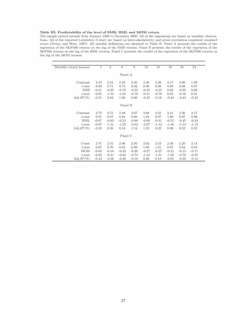
Table III: Predictability of the level of SMB, HML and MOM return.The sample period extends from January 1990 to December 2008. All of the regressions are based on monthly observa-tions. All of the reported t-statistics (t-stat) are based on heteroskedasticity and serial correlation consistent standarderrors (Newey and West, 1987). All variable definitions are identical to Table II. Panel A presents the results of theregression of the S&P500 returns on the lag of the SMB returns. Panel B presents the results of the regression of theS&P500 returns on the lag of the HML returns. Panel C presents the results of the regression of the S&P500 returns onthe lag of the MOM returns.

Monthly return horizon 1 3 6 9 12 15 18 21 24

Panel A

Constant 2.43 2.34 2.22 2.30 2.36 2.26 2.17 2.06 1.98t-stat 0.69 0.71 0.74 0.82 0.90 0.90 0.89 0.88 0.87SMB -0.51 -0.95 -0.75 -0.35 -0.23 -0.25 0.02 -0.05 0.06t-stat -0.65 -1.55 -1.65 -0.76 -0.51 -0.70 0.05 -0.16 0.21

Adj.R2(%) -0.31 0.83 1.06 0.00 -0.23 -0.16 -0.44 -0.43 -0.43

Panel B

Constant 2.75 2.75 2.48 2.67 2.68 2.45 2.41 2.26 2.17t-stat 0.81 0.87 0.84 0.98 1.04 0.97 1.00 0.97 0.96HML -0.67 -0.83 -0.53 -0.80 -0.69 -0.41 -0.55 -0.45 -0.43t-stat -0.67 -1.51 -1.25 -2.62 -2.07 -1.12 -1.48 -1.13 -1.13

Adj.R2(%) -0.25 0.38 0.18 1.54 1.25 0.22 0.90 0.52 0.53

Panel C

Const 2.47 2.55 2.46 2.50 2.62 2.53 2.36 2.20 2.14t-stat 0.67 0.76 0.82 0.89 1.00 1.01 0.97 0.94 0.94MOM -0.02 -0.18 -0.22 -0.20 -0.27 -0.27 -0.21 -0.15 -0.17t-stat -0.02 -0.41 -0.83 -0.74 -1.24 -1.31 -1.02 -0.76 -0.95

Adj.R2(%) -0.44 -0.36 -0.20 -0.18 0.08 0.18 -0.05 -0.22 -0.12

27

Table IV: Variance series regressions.The sample period extends from January 1990 to December 2008. All of the regressions are based on monthly observa-tions. All of the reported t-statistics (t-stat) are based on heteroskedasticity and serial correlation consistent standarderrors (Newey and West, 1987). All variable definitions are identical to Table II. Panel A presents the results fromthe regression of the S&P500 returns on the lag of the market realized volatility. Panel B presents the results fromthe regression of the S&P500 returns on the lag of the variance risk premium. Panel C presents the results from theregression of the S&P500 returns on the lag of the SMB variance. Panel D presents the results from the regression ofthe S&P500 returns on the lag of the HML variance. Panel E presents the results from the regression of the S&P500returns on the lag of the MOM variance.

Panel A

Monthly return horizon 1 3 6 9 12 15 18 21 24

Constant 5.87 3.99 3.57 3.62 3.65 3.40 3.27 3.11 2.96t-stat 1.95 1.41 1.42 1.62 1.71 1.67 1.65 1.59 1.54

σ2M -0.18 -0.08 -0.07 -0.07 -0.07 -0.06 -0.06 -0.05 -0.05

t-stat -2.46 -2.25 -2.33 -1.92 -1.79 -1.70 -1.62 -1.62 -1.60Adj.R2(%) 1.44 0.72 1.04 1.56 1.76 1.48 1.59 1.55 1.46

Panel B

Monthly return horizon 1 3 6 9 12 15 18 21 24

Constant -5.72 -4.12 -1.89 -0.64 -0.14 -0.11 0.21 0.34 0.36t-stat -1.66 -1.30 -0.70 -0.27 -0.06 -0.05 0.09 0.16 0.17

σ2∗M − σ2

M 0.48 0.38 0.24 0.17 0.15 0.14 0.11 0.10 0.09t-stat 4.47 3.30 2.74 2.37 2.33 2.25 2.18 2.12 2.05

Adj. R2(%) 3.24 6.02 4.53 3.02 2.48 2.48 1.76 1.40 1.31

Panel C

Monthly return horizon 1 3 6 9 12 15 18 21 24

Constant 7.70 4.58 3.56 3.95 4.24 3.92 4.06 3.78 3.67t-stat 2.30 1.55 1.20 1.37 1.51 1.46 1.54 1.47 1.47

σ2SMB -0.83 -0.35 -0.21 -0.26 -0.30 -0.26 -0.30 -0.27 -0.27t-stat -1.76 -1.28 -1.39 -2.17 -2.23 -2.08 -1.94 -2.11 -2.16

Adj. R2(%) 1.59 0.55 0.23 0.99 1.70 1.43 2.33 2.00 2.12

Panel D

Monthly return horizon 1 3 6 9 12 15 18 21 24

Constant 9.55 8.22 6.35 6.19 5.70 5.58 5.52 5.43 5.18t-stat 2.94 3.00 2.28 2.24 2.12 2.15 2.19 2.20 2.15

σ2HML -1.08 -0.89 -0.62 -0.59 -0.50 -0.50 -0.51 -0.51 -0.49t-stat -2.78 -3.59 -4.89 -5.02 -4.53 -4.29 -3.78 -3.57 -3.52

Adj. R2(%) 4.94 9.69 9.08 11.18 9.48 10.53 12.12 13.26 12.92

Panel E

Monthly return horizon 1 3 6 9 12 15 18 21 24

Constant 7.56 7.61 6.55 6.06 5.70 5.41 5.26 4.79 4.46t-stat 2.47 2.75 2.53 2.50 2.42 2.33 2.30 2.09 1.96

σ2MOM -0.41 -0.42 -0.34 -0.30 -0.26 -0.25 -0.25 -0.22 -0.20t-stat -3.66 -3.25 -4.12 -4.37 -4.51 -4.19 -3.86 -3.73 -3.68

Adj. R2(%) 3.61 11.40 14.84 15.34 14.01 13.96 15.13 12.64 11.18

28

Table V: Correlation series regressions.The sample period extends from January 1990 to December 2008. All of the regressions are based on monthly observa-tions. All of the reported t-statistics (t-stat) are based on heteroskedasticity and serial correlation consistent standarderrors (Newey and West, 1987). All variable definitions are identical to Table II.

Panel A

Monthly return horizon 1 3 6 9 12 15 18 21 24

Constant 1.89 1.35 1.37 0.84 0.95 0.76 0.67 0.53 0.40t-stat 0.57 0.41 0.46 0.29 0.35 0.29 0.27 0.22 0.17

ρM,SMB -3.84 -6.98 -5.93 -9.96 -9.63 -10.26 -10.14 -10.42 -10.71t-stat -0.65 -1.41 -1.41 -2.49 -2.60 -2.84 -2.93 -3.02 -3.06

Adj. R2(%) -0.31 0.80 1.26 6.12 6.69 8.61 9.40 10.78 12.32

Panel BMonthly return horizon 1 3 6 9 12 15 18 21 24

Constant -5.94 -6.67 -3.73 -2.38 -2.37 -1.69 -1.38 -1.09 -0.44t-stat -0.84 -1.05 -0.78 -0.59 -0.64 -0.46 -0.39 -0.32 -0.14

ρM,HML -18.73 -20.19 -13.33 -10.46 -10.59 -8.85 -7.92 -7.03 -5.39t-stat -1.42 -1.79 -1.65 -1.56 -1.78 -1.45 -1.31 -1.20 -0.99

Adj. R2(%) 1.55 6.01 4.91 4.05 4.91 3.74 3.28 2.73 1.56

Panel CMonthly return horizon 1 3 6 9 12 15 18 21 24

Constant 0.38 0.24 0.05 0.48 0.86 0.90 1.00 1.18 1.31t-stat 0.09 0.06 0.02 0.15 0.29 0.33 0.39 0.49 0.58

ρM,MOM 12.85 13.27 13.62 11.38 9.40 8.53 7.25 5.50 4.17t-stat 1.57 1.86 2.19 2.03 1.87 1.84 1.74 1.44 1.18

Adj. R2(%) 1.42 5.09 10.65 10.12 7.94 7.27 5.75 3.41 1.94

Panel DMonthly return horizon 1 3 6 9 12 15 18 21 24

Constant 4.27 3.65 3.65 3.82 3.72 3.60 3.45 3.27 3.11t-stat 1.25 1.13 1.29 1.53 1.55 1.55 1.57 1.56 1.55

ρSMB,HML 18.55 12.99 14.31 15.43 13.73 13.57 13.08 12.35 11.52t-stat 2.01 1.96 2.45 3.01 2.89 3.07 3.05 2.85 2.50

Adj. R2(%) 1.10 1.66 4.42 7.27 6.66 7.32 7.58 7.27 6.79

Panel EMonthly return horizon 1 3 6 9 12 15 18 21 24

Constant 2.79 2.47 2.43 2.43 2.45 2.32 2.22 2.11 2.06t-stat 0.80 0.74 0.80 0.86 0.90 0.89 0.89 0.88 0.89

ρSMB,MOM -9.37 -2.32 -5.14 -3.39 -2.12 -1.27 -1.61 -1.18 -2.16t-stat -1.11 -0.32 -0.90 -0.62 -0.39 -0.24 -0.33 -0.26 -0.49

Adj. R2(%) 0.06 -0.36 0.36 0.03 -0.23 -0.36 -0.29 -0.35 -0.12

Panel FMonthly return horizon 1 3 6 9 12 15 18 21 24

Constant 2.48 2.40 1.98 2.19 2.32 2.14 2.03 1.98 1.97t-stat 0.72 0.76 0.67 0.79 0.90 0.87 0.85 0.86 0.89

ρHML,MOM 0.26 0.26 -3.19 -1.46 -0.68 -1.60 -1.64 -1.06 -0.12t-stat 0.03 0.04 -0.68 -0.35 -0.16 -0.38 -0.41 -0.28 -0.03

Adj. R2(%) -0.44 -0.44 0.17 -0.27 -0.40 -0.17 -0.12 -0.30 -0.44

29

Table VI: Multivariate regressions without variance risk premium.The sample period extends from January 1990 to December 2008. All of the regressions are based on monthly observa-tions. All of the reported t-statistics (t-stat) are based on heteroskedasticity and serial correlation consistent standarderrors (Newey and West, 1987). All variable definitions are identical to Table II.

Const. σ2HML σ2

MOM ρM,SMB ρM,HML ρM,MOM

1 Month

Coeff -2.62 -1.29 0.14 0.28 -22.83 9.90t-stat -0.50 -1.96 0.49 0.05 -2.19 1.31

Adj. R2(%) 8.85

3 Months

Coeff -3.18 -0.78 -0.04 -3.20 -20.29 9.75t-stat -0.82 -2.82 -0.24 -0.74 -3.56 1.72

Adj. R2(%) 20.96

6 Months

Coeff -1.47 -0.34 -0.12 -4.28 -11.31 10.68t-stat -0.41 -1.34 -0.98 -1.38 -3.02 2.24

Adj. R2(%) 24.79

9 Months

Coeff -0.56 -0.37 -0.07 -9.14 -7.39 9.70t-stat -0.17 -1.46 -0.71 -3.20 -2.24 2.25

Adj. R2(%) 29.19

12 Months

Coeff -0.60 -0.30 -0.08 -8.57 -7.52 7.85t-stat -0.19 -1.32 -0.90 -3.12 -2.19 2.02

Adj. R2(%) 27.08

15 Months

Coeff 0.05 -0.32 -0.06 -9.54 -5.65 7.27t-stat 0.01 -1.70 -0.90 -3.60 -1.39 2.16

Adj. R2(%) 28.11

18 Months

Coeff 0.75 -0.32 -0.07 -9.36 -4.73 5.81t-stat 0.23 -1.84 -1.05 -3.74 -1.11 1.99

Adj. R2(%) 28.60

21 Months

Coeff 0.91 -0.43 -0.02 -9.60 -4.56 4.60t-stat 0.29 -2.15 -0.25 -3.81 -1.08 1.80

Adj. R2(%) 28.0124 Months

Coeff 1.60 -0.42 -0.01 -10.12 -2.76 3.46t-stat 0.55 -2.40 -0.24 -3.75 -0.73 1.47

Adj. R2(%) 27.16

30

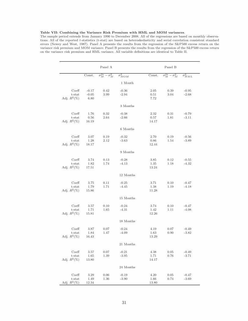
Table VII: Combining the Variance Risk Premium with HML and MOM variances.The sample period extends from January 1990 to December 2008. All of the regressions are based on monthly observa-tions. All of the reported t-statistics (t-stat) are based on heteroskedasticity and serial correlation consistent standarderrors (Newey and West, 1987). Panel A presents the results from the regression of the S&P500 excess return on thevariance risk premium and MOM variance. Panel B presents the results from the regression of the S&P500 excess returnon the variance risk premium and HML variance. All variable definitions are identical to Table II.

Panel A Panel B

Const. σ2∗M − σ2

M σ2MOM Const. σ2∗

M − σ2M σ2

HML

1 Month

Coeff -0.17 0.42 -0.36 2.05 0.39 -0.95t-stat -0.05 3.99 -2.94 0.51 3.04 -2.68

Adj. R2(%) 6.80 7.72

3 Months

Coeff 1.76 0.32 -0.38 2.32 0.31 -0.79t-stat 0.56 2.64 -2.66 0.57 1.81 -3.11

Adj. R2(%) 16.19 14.17

6 Months

Coeff 3.07 0.19 -0.32 2.70 0.19 -0.56t-stat 1.28 2.12 -3.63 0.86 1.54 -3.89

Adj. R2(%) 18.17 12.44

9 Months

Coeff 3.74 0.13 -0.28 3.85 0.12 -0.55t-stat 1.82 1.74 -4.13 1.35 1.18 -4.32

Adj. R2(%) 17.51 13.24

12 Months

Coeff 3.75 0.11 -0.25 3.71 0.10 -0.47t-stat 1.79 1.71 -4.45 1.38 1.19 -4.18

Adj. R2(%) 15.86 11.28

15 Months

Coeff 3.57 0.10 -0.24 3.74 0.10 -0.47t-stat 1.71 1.65 -4.31 1.42 1.11 -4.08

Adj. R2(%) 15.81 12.26

18 Months

Coeff 3.87 0.07 -0.24 4.19 0.07 -0.49t-stat 1.84 1.47 -4.09 1.63 0.90 -3.82

Adj. R2(%) 16.43 13.29

21 Months

Coeff 3.57 0.07 -0.21 4.38 0.05 -0.49t-stat 1.65 1.39 -3.95 1.71 0.76 -3.71

Adj. R2(%) 13.80 14.17

24 Months

Coeff 3.29 0.06 -0.19 4.20 0.05 -0.47t-stat 1.49 1.36 -3.90 1.66 0.74 -3.69

Adj. R2(%) 12.34 13.80

31

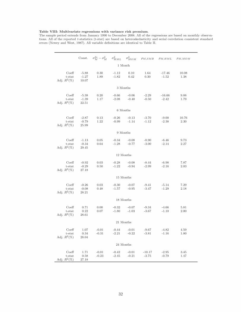
Table VIII: Multivariate regressions with variance risk premium.The sample period extends from January 1990 to December 2008. All of the regressions are based on monthly observa-tions. All of the reported t-statistics (t-stat) are based on heteroskedasticity and serial correlation consistent standarderrors (Newey and West, 1987). All variable definitions are identical to Table II.

Const. σ2∗M − σ2

M σ2HML σ2

MOM ρM,SMB ρM,HML ρM,MOM

1 Month

Coeff -5.88 0.30 -1.12 0.10 1.64 -17.46 10.08t-stat -1.27 1.89 -1.82 0.42 0.30 -1.52 1.38

Adj. R2(%) 10.07

3 Months

Coeff -5.38 0.20 -0.66 -0.06 -2.29 -16.66 9.88t-stat -1.39 1.17 -2.08 -0.40 -0.50 -2.42 1.79

Adj. R2(%) 22.51

6 Months

Coeff -2.87 0.13 -0.26 -0.13 -3.70 -9.00 10.76t-stat -0.79 1.22 -0.99 -1.14 -1.12 -2.38 2.30

Adj. R2(%) 25.99

9 Months

Coeff -1.13 0.05 -0.34 -0.08 -8.90 -6.46 9.73t-stat -0.34 0.64 -1.28 -0.77 -3.00 -2.14 2.27

Adj. R2(%) 29.45

12 Months

Coeff -0.92 0.03 -0.28 -0.08 -8.44 -6.98 7.87t-stat -0.29 0.50 -1.22 -0.94 -2.99 -2.16 2.03

Adj. R2(%) 27.18

15 Months

Coeff -0.26 0.03 -0.30 -0.07 -9.41 -5.14 7.29t-stat -0.08 0.48 -1.57 -0.95 -3.47 -1.29 2.18

Adj. R2(%) 28.21

18 Months

Coeff 0.71 0.00 -0.32 -0.07 -9.34 -4.66 5.81t-stat 0.22 0.07 -1.80 -1.03 -3.67 -1.10 2.00

Adj. R2(%) 28.61

21 Months

Coeff 1.07 -0.01 -0.44 -0.01 -9.67 -4.82 4.59t-stat 0.34 -0.31 -2.21 -0.22 -3.81 -1.16 1.80

Adj. R2(%) 28.04

24 Months

Coeff 1.71 -0.01 -0.42 -0.01 -10.17 -2.95 3.45t-stat 0.58 -0.23 -2.45 -0.21 -3.75 -0.79 1.47

Adj. R2(%) 27.18

32

Table IX: Univariate regressions using CAYt, log(Pt/Et), and log(Pt/Dt).The sample period extends from January 1990 to December 2008. All of the regressions are based on monthly observa-tions. All of the reported t-statistics (t-stat) are based on heteroskedasticity and serial correlation consistent standarderrors (Newey and West, 1987). All variable definitions are identical to Table II.

Monthly return horizon 1 3 6 9 12 15 18 21 24

log(Pt/Et)

Const 22.20 25.16 26.56 35.18 46.03 51.62 55.08 59.18 62.55t-stat 0.51 0.67 0.81 1.24 1.81 2.19 2.50 2.79 3.06Slope -6.09 -7.03 -7.50 -10.14 -13.47 -15.22 -16.32 -17.62 -18.68t-stat -0.46 -0.61 -0.74 -1.14 -1.68 -2.04 -2.33 -2.61 -2.88

Adj. R2(%) -0.34 -0.06 0.38 1.62 3.79 5.61 7.30 9.30 11.36

log(Pt/Dt)

Const 44.40 46.25 46.26 52.53 60.73 63.98 65.69 67.78 69.43t-stat 1.15 1.37 1.59 2.15 2.80 3.15 3.40 3.58 3.75Slope -10.68 -11.17 -11.21 -12.79 -14.86 -15.71 -16.17 -16.73 -17.17t-stat -1.09 -1.30 -1.50 -2.01 -2.61 -2.94 -3.18 -3.37 -3.56

Adj. R2(%) 0.05 1.05 2.42 4.64 7.54 9.54 11.32 13.16 15.00

log(CAY t)

Const 1.40 1.29 1.18 1.17 1.14 0.98 0.81 0.64 0.49t-stat 0.40 0.39 0.39 0.42 0.44 0.40 0.35 0.30 0.24Slope 2.91 3.02 2.95 3.17 3.41 3.57 3.74 3.94 4.11t-stat 2.27 2.55 2.87 3.36 3.54 3.70 3.91 4.25 4.61

Adj. R2(%) 0.92 3.63 6.96 11.20 15.26 18.83 23.06 27.70 32.54

33

Table X: Combining the predictors when the return horizon is one month.The sample period extends from January 1990 to December 2008. All of the regressions are based on monthly obser-vations. The return horizon is one month. All of the reported t-statistics (t-stat) are based on heteroskedasticity andserial correlation consistent standard errors (Newey and West, 1987). All variable definitions are identical to Table II.

Const. σ2∗M − σ2

M σ2HML σ2

MOM CAY t

1 month

Coeff -5.72 0.48t-stat -1.66 4.47

Adj. R2(%) 3.24

Coeff 9.55 -1.08t-stat 2.94 -2.78

Adj. R2(%) 4.94

Coeff 7.56 -0.41t-stat 2.47 -3.66

Adj. R2(%) 3.61

Coeff 1.40 2.91t-stat 0.40 2.27

Adj. R2(%) 0.92

Coeff -6.20 0.45 2.46t-stat -1.63 4.43 1.85

Adj. R2(%) 4.63

Coeff 8.40 -1.02 2.18t-stat 2.50 -2.49 1.76

Adj. R2(%) 6.10

Coeff 6.43 -0.38 2.10t-stat 2.09 -3.42 1.74

Adj. R2(%) 4.72

Coeff 2.05 0.39 -0.95t-stat 0.51 3.04 -2.68

Adj. R2(%) 7.72

Coeff 1.34 0.37 -0.91 1.89t-stat 0.34 3.23 -2.63 1.53

Adj. R2(%) 7.29

Coeff -0.87 0.40 -0.34 1.78t-stat -0.27 4.15 -3.17 1.43

Adj. R2(%) 8.28

Coeff 1.50 0.37 -0.74 -0.10 1.80t-stat 0.41 3.41 -1.30 -0.54 1.49

Adj. R2(%) 8.38

34

Table XI: Combining the predictors when the return horizon is three months.The sample period extends from January 1990 to December 2008. All of the regressions are based on monthly observa-tions. The returns horizon is 3 months. All of the reported t-statistics (t-stat) are based on heteroskedasticity and serialcorrelation consistent standard errors (Newey and West, 1987). All variable definitions are identical to Table II.

Const. σ2∗M − σ2

M σ2HML σ2

MOM CAY t

3 months

Coeff -4.12 0.38t-stat -1.30 3.30

Adj. R2(%) 6.02

Coeff 8.22 -0.89t-stat 3.00 -3.59

Adj. R2(%) 9.69

Coeff 7.61 -0.42t-stat 2.75 -3.25

Adj. R2(%) 11.40

Coeff 1.29 3.02t-stat 0.39 2.55

Adj. R2(%) 3.63

Coeff -4.63 0.35 2.67t-stat -1.41 3.34 2.16

Adj. R2(%) 9.58

Coeff 6.94 -0.83 2.43t-stat 2.54 -3.19 2.27

Adj. R2(%) 12.67

Coeff 6.43 -0.38 2.19t-stat 2.31 -2.99 2.09

Adj. R2(%) 13.86

Coeff 2.32 0.31 -0.79t-stat 0.57 1.81 -3.11

Adj. R2(%) 14.17

Coeff 1.49 0.29 -0.74 2.20t-stat 0.37 1.77 -2.95 1.98

Adj. R2(%) 16.28

Coeff 0.99 0.30 -0.35 1.95t-stat 0.31 2.60 -2.72 1.80

Adj. R2(%) 17.82

Coeff 1.92 0.29 -0.29 -0.26 1.96t-stat 0.52 2.09 -0.82 -1.43 1.82

Adj. R2(%) 18.29

35

Table XII: Combining the predictors when the return horizon is six months.The sample period extends from January 1990 to December 2008. All of the regressions are based on monthly observa-tions. The returns horizon is 6 months. All of the reported t-statistics (t-stat) are based on heteroskedasticity and serialcorrelation consistent standard errors (Newey and West, 1987). All variable definitions are identical to Table II.

Const. σ2∗M − σ2

M σ2HML σ2

MOM CAY t

6 months

Coeff -1.89 0.24t-stat -0.70 2.74

Adj. R2(%) 4.53

Coeff 6.35 -0.62t-stat 2.28 -4.89

Adj. R2(%) 9.08

Coeff 6.55 -0.34t-stat 2.53 -4.12

Adj. R2(%) 14.84

Coeff 1.18 2.95t-stat 0.39 2.87

Adj. R2(%) 6.96

Coeff -2.41 0.21 2.74t-stat -0.82 2.62 2.60

Adj. R2(%) 11.25

Coeff 5.01 -0.56 2.55t-stat 1.78 -4.10 2.71

Adj. R2(%) 14.89

Coeff 5.32 -0.31 2.28t-stat 2.04 -3.77 2.53

Adj. R2(%) 19.49

Coeff 2.70 0.19 -0.56t-stat 0.86 1.54 -3.89

Adj. R2(%) 12.44

Coeff 1.80 0.17 -0.51 2.42t-stat 0.54 1.45 -3.50 2.49

Adj. R2(%) 17.28

Coeff 2.22 0.17 -0.29 2.15t-stat 0.87 1.98 -3.50 2.31

Adj. R2(%) 21.93

Coeff 2.27 0.17 -0.01 -0.29 2.15t-stat 0.79 1.87 -0.04 -1.83 2.31

Adj. R2(%) 21.94

36

Table XIII: Combining the predictors when the return horizon is nine months.The sample period extends from January 1990 to December 2008. All of the regressions are based on monthly observa-tions. The returns horizon is 9 months. All of the reported t-statistics (t-stat) are based on heteroskedasticity and serialcorrelation consistent standard errors (Newey and West, 1987). All variable definitions are identical to Table II.

Const. σ2∗M − σ2

M σ2HML σ2

MOM CAY t

9 months

Coeff -0.64 0.17t-stat -0.27 2.37

Adj. R2(%) 3.02

Coeff 6.19 -0.59t-stat 2.24 -5.02

Adj. R2(%) 11.18

Coeff 6.06 -0.30t-stat 2.50 -4.37

15.34

Coeff 1.17 3.17t-stat 0.42 3.36

Adj. R2(%) 11.20

Coeff -1.22 0.14 3.03t-stat -0.45 1.99 3.16

Adj. R2(%) 13.93

Coeff 4.72 -0.52 2.79t-stat 1.69 -4.57 3.20

Adj. R2(%) 20.44

Coeff 4.65 -0.26 2.60t-stat 1.90 -4.19 3.12

Adj. R2(%) 23.31

Coeff 3.85 0.12 -0.55t-stat 1.35 1.18 -4.32

Adj. R2(%) 13.24

Coeff 2.83 0.10 -0.49 2.72t-stat 0.91 1.01 -3.78 3.05

Adj. R2(%) 21.57

Coeff 2.74 0.11 -0.25 2.52t-stat 1.18 1.44 -3.97 2.95

Adj. R2(%) 24.58

Coeff 3.17 0.10 -0.13 -0.21 2.52t-stat 1.13 1.21 -0.37 -1.40 2.98

Adj. R2(%) 24.84

37

Table XIV: Combining the predictors when the return horizon is twelve months.The sample period extends from January 1990 to December 2008. All of the regressions are based on monthly observa-tions. The return horizon is 12 months. All of the reported t-statistics (t-stat) are based on heteroskedasticity and serialcorrelation consistent standard errors (Newey and West, 1987). All variable definitions are identical to Table II.

Const. σ2∗M − σ2

M σ2HML σ2

MOM CAY t

12 months

Coeff -0.14 0.15t-stat -0.06 2.33

Adj. R2(%) 2.48

Coeff 5.70 -0.50t-stat 2.12 -4.53

Adj. R2(%) 9.48

Coeff 5.70 -0.26t-stat 2.42 -4.51

Adj. R2(%) 14.01

Coeff 1.14 3.41t-stat 0.44 3.54

Adj. R2(%) 15.26

Coeff -0.78 0.11 3.30t-stat -0.30 1.92 3.39

Adj. R2(%) 17.39

Coeff 4.07 -0.43 3.11t-stat 1.50 -4.19 3.36

Adj. R2(%) 22.61

Coeff 4.12 -0.22 2.93t-stat 1.73 -4.47 3.29

Adj. R2(%) 25.57

Coeff 3.71 0.10 -0.47t-stat 1.38 1.19 -4.18

Adj. R2(%) 11.28

Coeff 2.57 0.08 -0.40 3.04t-stat 0.86 0.99 -3.53 3.26

Adj. R2(%) 23.43

Coeff 2.62 0.08 -0.21 2.86t-stat 1.10 1.35 -4.20 3.17

Adj. R2(%) 26.48

Coeff 2.87 0.08 -0.08 -0.19 2.87t-stat 1.04 1.19 -0.27 -1.56 3.19

Adj. R2(%) 26.59

38

Table XV: Combining the correlation series with the CAYt and variance risk premium.The sample period extends from January 1990 to December 2008. All of the regressions are based on monthly observa-tions. All of the reported t-statistics (t-stat) are based on heteroskedasticity and serial correlation consistent standarderrors (Newey and West, 1987). All variable definitions are identical to Table II.

Const. ρM,MOM σ2∗M − σ2

M CAY t

1 monthCoeff 0.38 12.85t-stat 0.09 1.57

Adj. R2(%) 1.42

Coeff -5.72 0.48t-stat -1.66 4.47

Adj. R2(%) 3.24

Coeff 1.40 2.91t-stat 0.40 2.27

Adj. R2(%) 0.92

Coeff -0.78 13.26 3.04t-stat -0.20 1.67 2.41

Adj. R2(%) 3.33

Coeff -8.52 13.54 0.46 2.59t-stat -2.16 1.87 5.04 2.02

Adj. R2(%) 6.693 months

Coeff 0.24 13.27t-stat 0.06 1.86

Adj. R2(%) 5.51

Coeff -4.12 0.38t-stat -1.30 3.30

Adj. R2(%) 6.02

Coeff 1.29 3.02t-stat 0.39 2.55

Adj. R2(%) 3.63

Coeff -0.96 13.70 3.15t-stat -0.26 2.02 2.70

Adj. R2(%) 9.92

Coeff -7.02 13.91 0.36 2.79t-stat -2.08 2.30 2.89 2.33

Adj. R2(%) 15.636 months

Coeff 0.05 13.62t-stat 0.02 2.19

Adj. R2(%) 10.65

Coeff -1.89 0.24t-stat -0.70 2.74

Adj. R2(%) 4.53

Coeff 1.18 2.95t-stat 0.39 2.87

Adj. R2(%) 6.96

Coeff -1.13 14.04 3.08t-stat -0.34 2.41 3.06

Adj. R2(%) 19.10

Coeff -4.85 14.17 0.22 2.87t-stat -1.57 2.62 2.22 2.81

Adj. R2(%) 23.19This table continues on the next page....

39

.

Const. ρM,MOM σ2∗M − σ2

M CAY t

9 months

Coeff 0.48 11.38t-stat 0.15 2.03

Adj. R2(%) 10.12

Coeff -0.64 0.17t-stat -0.27 2.37

Adj. R2(%) 3.02

Coeff 1.17 3.17t-stat 0.42 3.36

Adj. R2(%) 11.20

Coeff -0.78 11.82 3.28t-stat -0.26 2.25 3.62

Adj. R2(%) 22.93

Coeff -3.27 11.91 0.15 3.13t-stat -1.14 2.36 1.83 3.42

Adj. R2(%) 25.44

12 months

Coeff 0.86 9.40t-stat 0.29 1.87

Adj. R2(%) 7.94

Coeff -0.14 0.15t-stat -0.06 2.33

Adj. R2(%) 2.48

Coeff 1.14 3.41t-stat 0.44 3.54

Adj. R2(%) 15.26

Coeff -0.49 9.88 3.51t-stat -0.17 2.10 3.79

Adj. R2(%) 24.84

Coeff -2.49 9.95 0.12 3.39t-stat -0.91 2.18 1.77 3.64

Adj. R2(%) 26.72

40

Table XVI: Stock return predictability over different sample periods: Adjusted R-squared.This table presents the adjusted R-squared (%) obtained from regression the S&P500 excess return on each of thepredictor variables. I report the adjusted-R-squared for different sample periods. All variable definitions are identical toTable II.

Sample period σ2M σ2

SMB σ2HML σ2

MOM ρM,MOM CAY log(P/E) log(P/D)

1 Month

1990-2008 1.44 1.59 4.94 3.62 1.42 0.92 -0.34 0.051987-2008 2.82 2.80 4.40 3.56 0.14 0.78 -0.26 0.051980-2008 1.94 1.78 3.20 2.55 0.05 0.72 -0.22 -0.071970-2008 1.28 0.99 2.20 1.48 0.14 1.54 -0.18 -0.101970-1990 0.52 0.45 0.51 -0.17 -0.36 1.60 0.24 0.49

3 Months

1990-2008 0.72 0.55 9.69 11.40 5.09 3.63 -0.06 1.051987-2008 0.20 -0.23 6.95 8.26 2.30 2.60 -0.02 0.811980-2008 0.11 -0.25 6.11 6.08 0.57 2.21 0.03 0.551970-2008 -0.10 -0.21 3.09 3.37 0.47 3.91 -0.09 0.161970-1990 0.04 0.01 -0.32 0.57 -0.00 3.56 1.63 2.50

6 Months

1990-2008 1.04 0.23 9.08 14.84 10.65 6.96 0.38 2.421987-2008 0.48 -0.22 7.02 11.76 5.27 6.16 0.29 1.9171980-2008 0.33 -0.24 6.26 8.17 0.85 4.52 0.45 1.491970-2008 -0.07 -0.21 2.86 4.57 0.89 6.76 0.10 0.721970-1990 0.25 -0.04 0.03 1.10 0.41 6.48 2.73 5.27

12 Months

1990-2008 1.76 1.70 9.48 14.01 7.94 15.26 3.79 7.541987-2008 0.74 -0.03 7.58 11.47 3.03 13.50 2.30 5.281980-2008 0.66 -0.08 6.29 8.74 -0.29 10.45 1.15 2.941970-2008 0.13 -0.20 3.06 5.47 -0.10 13.88 0.63 1.921970-1990 0.15 0.08 0.66 -0.03 3.98 12.41 4.81 9.78

41

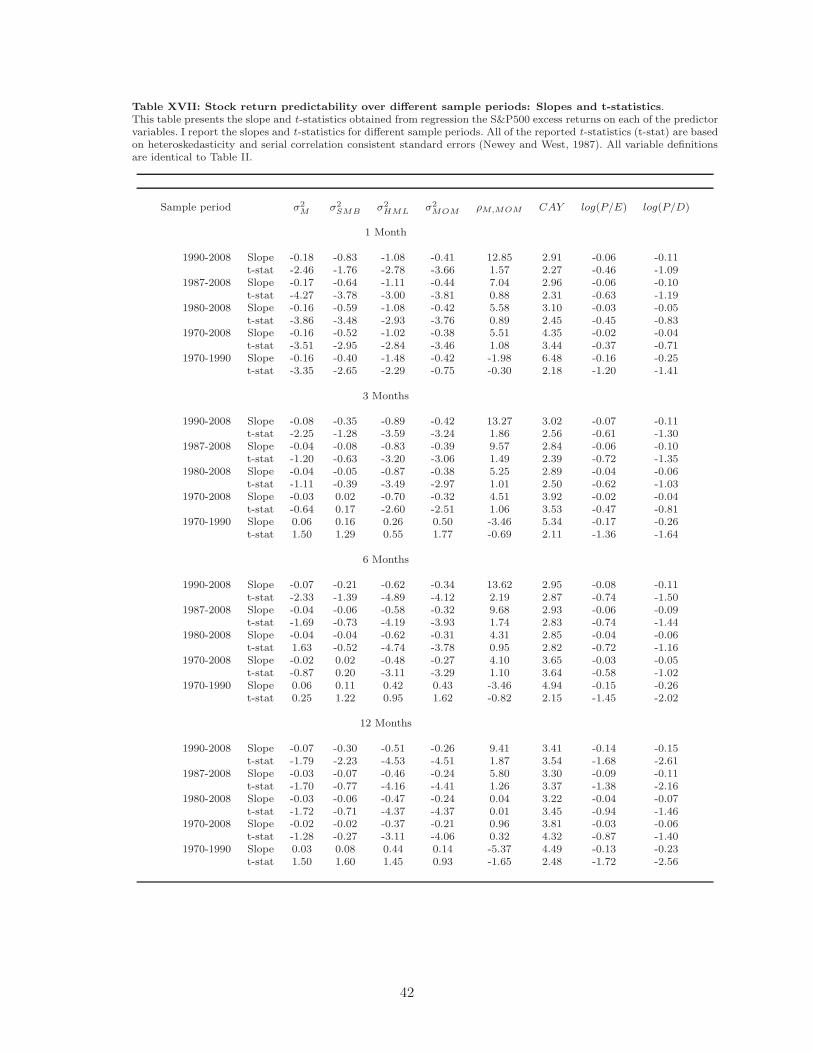
Table XVII: Stock return predictability over different sample periods: Slopes and t-statistics.This table presents the slope and t-statistics obtained from regression the S&P500 excess returns on each of the predictorvariables. I report the slopes and t-statistics for different sample periods. All of the reported t-statistics (t-stat) are basedon heteroskedasticity and serial correlation consistent standard errors (Newey and West, 1987). All variable definitionsare identical to Table II.

Sample period σ2M σ2

SMB σ2HML σ2

MOM ρM,MOM CAY log(P/E) log(P/D)

1 Month

1990-2008 Slope -0.18 -0.83 -1.08 -0.41 12.85 2.91 -0.06 -0.11t-stat -2.46 -1.76 -2.78 -3.66 1.57 2.27 -0.46 -1.09

1987-2008 Slope -0.17 -0.64 -1.11 -0.44 7.04 2.96 -0.06 -0.10t-stat -4.27 -3.78 -3.00 -3.81 0.88 2.31 -0.63 -1.19

1980-2008 Slope -0.16 -0.59 -1.08 -0.42 5.58 3.10 -0.03 -0.05t-stat -3.86 -3.48 -2.93 -3.76 0.89 2.45 -0.45 -0.83

1970-2008 Slope -0.16 -0.52 -1.02 -0.38 5.51 4.35 -0.02 -0.04t-stat -3.51 -2.95 -2.84 -3.46 1.08 3.44 -0.37 -0.71

1970-1990 Slope -0.16 -0.40 -1.48 -0.42 -1.98 6.48 -0.16 -0.25t-stat -3.35 -2.65 -2.29 -0.75 -0.30 2.18 -1.20 -1.41

3 Months

1990-2008 Slope -0.08 -0.35 -0.89 -0.42 13.27 3.02 -0.07 -0.11t-stat -2.25 -1.28 -3.59 -3.24 1.86 2.56 -0.61 -1.30

1987-2008 Slope -0.04 -0.08 -0.83 -0.39 9.57 2.84 -0.06 -0.10t-stat -1.20 -0.63 -3.20 -3.06 1.49 2.39 -0.72 -1.35

1980-2008 Slope -0.04 -0.05 -0.87 -0.38 5.25 2.89 -0.04 -0.06t-stat -1.11 -0.39 -3.49 -2.97 1.01 2.50 -0.62 -1.03

1970-2008 Slope -0.03 0.02 -0.70 -0.32 4.51 3.92 -0.02 -0.04t-stat -0.64 0.17 -2.60 -2.51 1.06 3.53 -0.47 -0.81

1970-1990 Slope 0.06 0.16 0.26 0.50 -3.46 5.34 -0.17 -0.26t-stat 1.50 1.29 0.55 1.77 -0.69 2.11 -1.36 -1.64

6 Months

1990-2008 Slope -0.07 -0.21 -0.62 -0.34 13.62 2.95 -0.08 -0.11t-stat -2.33 -1.39 -4.89 -4.12 2.19 2.87 -0.74 -1.50

1987-2008 Slope -0.04 -0.06 -0.58 -0.32 9.68 2.93 -0.06 -0.09t-stat -1.69 -0.73 -4.19 -3.93 1.74 2.83 -0.74 -1.44

1980-2008 Slope -0.04 -0.04 -0.62 -0.31 4.31 2.85 -0.04 -0.06t-stat 1.63 -0.52 -4.74 -3.78 0.95 2.82 -0.72 -1.16

1970-2008 Slope -0.02 0.02 -0.48 -0.27 4.10 3.65 -0.03 -0.05t-stat -0.87 0.20 -3.11 -3.29 1.10 3.64 -0.58 -1.02

1970-1990 Slope 0.06 0.11 0.42 0.43 -3.46 4.94 -0.15 -0.26t-stat 0.25 1.22 0.95 1.62 -0.82 2.15 -1.45 -2.02

12 Months

1990-2008 Slope -0.07 -0.30 -0.51 -0.26 9.41 3.41 -0.14 -0.15t-stat -1.79 -2.23 -4.53 -4.51 1.87 3.54 -1.68 -2.61

1987-2008 Slope -0.03 -0.07 -0.46 -0.24 5.80 3.30 -0.09 -0.11t-stat -1.70 -0.77 -4.16 -4.41 1.26 3.37 -1.38 -2.16

1980-2008 Slope -0.03 -0.06 -0.47 -0.24 0.04 3.22 -0.04 -0.07t-stat -1.72 -0.71 -4.37 -4.37 0.01 3.45 -0.94 -1.46

1970-2008 Slope -0.02 -0.02 -0.37 -0.21 0.96 3.81 -0.03 -0.06t-stat -1.28 -0.27 -3.11 -4.06 0.32 4.32 -0.87 -1.40

1970-1990 Slope 0.03 0.08 0.44 0.14 -5.37 4.49 -0.13 -0.23t-stat 1.50 1.60 1.45 0.93 -1.65 2.48 -1.72 -2.56

42

Jan 90 Jan 94 Jan 98 Janv 02 Jan 06 Jan 100

50

100

150

200

250

300

350

400

450

500S&P 500 realized variance

Jan 90 Jan 94 Jan 98 Janv 02 Jan 06 Jan 100

10

20

30

40

50

60

70

80

90SMB variance

Jan 90 Jan 94 Jan 98 Janv 02 Jan 06 Jan 100

10

20

30

40

50

60

70

80HML variance

Jan 90 Jan 94 Jan 98 Janv 02 Jan 06 Jan 100

20

40

60

80

100

120

140

160

180

200MOM variance

Figure 1: Variance SeriesThis figure plots the realized variance (the top left panel) for the SP 500 market index, the SMBvariance (the top right panel), the HML variance ( (the bottom left panel) and MOM variance (thebottom right panel). The sample period is from January 1990 to December 2008.

43

Jan 90 Jan 94 Jan 98 Janv 02 Jan 06 Jan 10−200

−150

−100

−50

0

50

100

150Difference between implied and realized variances

Figure 2: Variance Risk Premium SeriesThis figure plots the variance risk premium (difference between the implied variance and the realizedvariance). The sample period is from January 1990 to December 2008.

44

Jan 90 Jan 94 Jan 98 Janv 02 Jan 06 Jan 10−1

−0.5

0

0.5

1ρ(RM,SMB)

Jan 90 Jan 94 Jan 98 Janv 02 Jan 06 Jan 10−1

−0.5

0

0.5

1ρ(RM,HML)

Jan 90 Jan 94 Jan 98 Janv 02 Jan 06 Jan 10−1

−0.5

0

0.5

1ρ(RM,MOM)

Jan 90 Jan 94 Jan 98 Janv 02 Jan 06 Jan 10−1

−0.5

0

0.5

1ρ(SMB,HML)

Jan 90 Jan 94 Jan 98 Janv 02 Jan 06 Jan 10−1

−0.5

0

0.5

1ρ(SMB,MOM)

Jan 90 Jan 94 Jan 98 Janv 02 Jan 06 Jan 10−1

−0.5

0

0.5

1ρ(HML,MOM)

Figure 3: Correlation SeriesThis figure plots the correlations among the market, the size, the book-to-market, and momentumfactor. I use daily returns to compute these correlation measures every month. The sample periodis from January 1990 to December 2008.

45

0 5 10 15 20 250

0.1

0.2

0.3

0.4

0.5

0.6

0.7

0.8Estimated slope coefficient and 95% confidence band

SlopeUpper boundLower bound

0 5 10 15 20 251

2

3

4

5

6

7

Horizons (months)

Estimated adjusted Rsquare (%)

σ2*M

−σ2M

Figure 4: Estimated Slopes and R2sThe figure shows the estimated slope coefficients and pointwise 95% confidence intervals along withthe corresponding R2 s from the regressions of the scaled h-period S&P 500 returns on the variancedifference. All of the regressions are based on monthly observations from January 1990 to December2008.

46

0 5 10 15 20 25−2

−1.8

−1.6

−1.4

−1.2

−1

−0.8

−0.6

−0.4

−0.2Estimated slope coefficient and 95% confidence band

SlopeLower boundUpper bound

0 5 10 15 20 254

5

6

7

8

9

10

11

12

13

14

Horizons (months)

Estimated adjusted Rsquare (%)

σ2HML

Figure 5: Estimated Slopes and R2sThe figure shows the estimated slope coefficients and pointwise 95% confidence intervals along withthe corresponding R2 s from the regressions of the scaled h-period S&P 500 returns on the HMLvariance. All of the regressions are based on monthly observations from January 1990 to December2008.

47

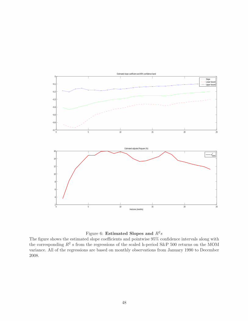
0 5 10 15 20 25−0.7

−0.6

−0.5

−0.4

−0.3

−0.2

−0.1

0Estimated slope coefficient and 95% confidence band

SlopeLower boundUpper bound

0 5 10 15 20 252

4

6

8

10

12

14

16

Horizons (months)

Estimated adjusted Rsquare (%)

σ2MOM

Figure 6: Estimated Slopes and R2sThe figure shows the estimated slope coefficients and pointwise 95% confidence intervals along withthe corresponding R2 s from the regressions of the scaled h-period S&P 500 returns on the MOMvariance. All of the regressions are based on monthly observations from January 1990 to December2008.

48

0 5 10 15 20 25−20

−15

−10

−5

0

5

10Estimated slope coefficient and 95% confidence band

SlopeLower boundUpper bound

0 5 10 15 20 25−2

0

2

4

6

8

10

12

14

Horizons (months)

Estimated adjusted Rsquare (%)

ρ(RM,SMB)

Figure 7: Estimated Slopes and R2sThe figure shows the estimated slope coefficients and pointwise 95% confidence intervals alongwith the corresponding R2 s from the regressions of the scaled h-period S&P 500 returns on thecorrelation ρM,SMB. All of the regressions are based on monthly observations from January 1990to December 2008.

49

0 5 10 15 20 25−50

−40

−30

−20

−10

0

10Estimated slope coefficient and 95% confidence band

SlopeLower boundUpper bound

0 5 10 15 20 251

2

3

4

5

6

7

Horizons (months)

Estimated adjusted Rsquare (%)

ρ(RM,HML)

Figure 8: Estimated Slopes and R2sThe figure shows the estimated slope coefficients and pointwise 95% confidence intervals alongwith the corresponding R2 s from the regressions of the scaled h-period S&P 500 returns on thecorrelation ρM,HML. All of the regressions are based on monthly observations from January 1990to December 2008.

50

0 5 10 15 20 25−5

0

5

10

15

20

25

30Estimated slope coefficient and 95% confidence band

SlopeLower boundUpper bound

0 5 10 15 20 251

2

3

4

5

6

7

8

9

10

11

Horizons (months)

Estimated adjusted Rsquare (%)

ρ(RM,MOM)

Figure 9: Estimated Slopes and R2sThe figure shows the estimated slope coefficients and pointwise 95% confidence intervals alongwith the corresponding R2 s from the regressions of the scaled h-period S&P 500 returns on thecorrelation ρM,MOM . All of the regressions are based on monthly observations from January 1990to December 2008.

51

0 5 10 15 20 250

5

10

15

20

25Estimated slope coefficient and 95% confidence band

SlopeLower boundUpper bound

0 5 10 15 20 251

2

3

4

5

6

7

8

9

Horizons (months)

Estimated adjusted Rsquare (%)

ρ(SMB,HML)

Figure 10: Estimated Slopes and R2sThe figure shows the estimated slope coefficients and pointwise 95% confidence intervals alongwith the corresponding R2 s from the regressions of the scaled h-period S&P 500 returns on thecorrelation ρSMB,HML. All of the regressions are based on monthly observations from January 1990to December 2008.

52

0 5 10 15 20 25−5

0

5

10

15

20

25

30

35

Horizons (months)

Estimated adjusted Rsquare (%)

log(Pt/Et)log(Pt/Dt)CAYt

σ2*M

−σ2M

0 5 10 15 20 25−5

0

5

10

15

20

25

30

35

Horizons (months)

Estimated adjusted Rsquare (%)

log(Pt/Et)log(Pt/Dt)CAYt

σ2SMB

0 5 10 15 20 25−5

0

5

10

15

20

25

30

35

Horizons (months)

Estimated adjusted Rsquare (%)

log(Pt/Et)log(Pt/Dt)CAYt

σ2HML

0 5 10 15 20 25−5

0

5

10

15

20

25

30

35

Horizons (months)

Estimated adjusted Rsquare (%)

log(Pt/Et)log(Pt/Dt)CAYt

σ2MOM

Figure 11: Estimated R2sThe figure shows the R2 s from the multivariate regressions of the scaled h-period S&P 500 returnson predictor variables. All of the regressions are based on monthly observations from January 1990to December 2008.

53

0 5 10 15 20 25−5

0

5

10

15

20

25

30

35

Horizons (months)

Estimated adjusted Rsquare (%)

log(Pt/Et)log(Pt/Dt)CAYtρ(RM,SMB)

0 5 10 15 20 25−5

0

5

10

15

20

25

30

35

Horizons (months)

Estimated adjusted Rsquare (%)

log(Pt/Et)log(Pt/Dt)CAYtρ(RM,HML)

0 5 10 15 20 25−5

0

5

10

15

20

25

30

35

Horizons (months)

Estimated adjusted Rsquare (%)

log(Pt/Et)log(Pt/Dt)CAYtρ(RM,MOM)

0 5 10 15 20 25−5

0

5

10

15

20

25

30

35

Horizons (months)

Estimated adjusted Rsquare (%)

log(Pt/Et)log(Pt/Dt)CAYtρ(SMB,HML)

Figure 12: Estimated R2sThe figure shows the R2 s from the multivariate regressions of the scaled h-period S&P 500 returnson predictor variables. All of the regressions are based on monthly observations from January 1990to December 2008.

54