The CAPM and Fama-French Models in Brazil ANNUAL MEETINGS/2008-… · The CAPM and Fama-French...

The CAPM and Fama-French Models inBrazil1

Fernando Daniel Chague2

Rodrigo D. L. S. Bueno3

Fundação Getulio VargasR. Itapeva, 474 - 7.o andar - Bela Vista

01332-000 - São Paulo - S.P.

December 2007

1The first author thanks CAPES and EESP-FGV for the financial support. The secondauthor thanks GVPesquisa for the financial support.

2MA in Economics, graduate student at University of North Caroline, Chapell Hill.Email: [email protected]

3Getulio Vargas Foundation, Sao Paulo and and CFC/FGV. [email protected]

Resumo

AbstractThis paper confronts the Capital Asset Pricing Model - CAPM - and the 3-Factor

Fama-French - FF - model using both Brazilian and US stock market data for thesame sample period (1999-2007). The US data will serve only as a benchmark forcomparative purposes. We use two competing econometric methods, the Gener-alized Method of Moments (GMM) by Hansen (1982) and the Iterative NonlinearSeemingly Unrelated Regression Estimation (ITNLSUR) by Burmeister and McElroy(1988). Both methods nest other options based on the procedure by Fama-MacBeth(1973). The estimations show that the FF model fits the Brazilian data better thanCAPM, however it is imprecise compared with the US analog. We argue that this isa consequence of an absence of clear-cut anomalies in Brazilian data, specially thoserelated to firm size. The tests on the efficiency of the models - nullity of interceptsand fitting of the cross-sectional regressions - presented mixed conclusions. Thetests on intercept failed to rejected the CAPM when Brazilian value-premium-wiseportfolios were used, contrasting with US data, a very well documented conclusion.The ITNLSUR has estimated an economically reasonable and statistically significantmarket risk premium for Brazil around 6.5% per year without resorting to any par-ticular data set aggregation. However, we could not find the same for the US dataduring identical period or even using a larger data set.JEL Classification: G12, C52, C12Key-words: CAPM, Fama-French, risk premium, ITNLSUR, GMMEFM Code: 310

1 Introduction

This paper confronts the Capital Asset Pricing Model - CAPM - and the 3-FactorFama-French - FF - model using both Brazilian and US stock market data for thesame sample period (1999-2007). The focus is on the Brazilian data analysis, sincethe results for the US’ are widely known. Therefore, the US data will serve only as abenchmark for comparative purposes. We use two competing econometric methods,the Generalized Method of Moments (GMM) by Hansen (1982) and the IterativeNonlinear Seemingly Unrelated Regression Estimation (ITNLSUR) by Burmeisterand McElroy (1988). Both methods nest other options like the Generalized LeastSquares (GLS), the Ordinary Least Squares (OLS) and the Weigthed Least Squares(WLS) frameworks based on the procedure by Fama-MacBeth (1973). AlthoughGMM method accounts for possible autocorrelated errors, it has a poor performancefor small samples. The ITNLSUR is strongly consistent and asymptotically normallydistributed and hence it is robust with respect to non-normal errors; however, whileit assumes heteroskedasticity errors, it does not takes into account possible errorautocorrelations.The estimations show that the FF model fits the Brazilian data better than

CAPM, however it is imprecise compared with the US analog. We argue that this isa consequence of an absence of clear-cut anomalies in Brazilian data, specially thoserelated to firm size. The tests on the efficiency of the models - nullity of interceptsand fitting of the cross-sectional regressions - presented mixed conclusions. Thetests on intercept failed to rejected the CAPM when Brazilian value-premium-wiseportfolios were used, contrasting with US data, a very well documented conclusion.The ITNLSUR has estimated an economically reasonable and statistically signifi-cant market risk premium for Brazil around 6.5% per year without resorting to anyparticular data set aggregation. However, we could not find the same for the USdata during identical period or even using a larger data set. These findings seem tocontradict the perception that market efficiency would unlikely prevail in an emergingmarket like Brazil but rather in economies like the US.The CAPMmodel of Sharpe (1964) and Lintner (1965) embodies successfully the

agents’ behavior features of Markowitz (1952), and establishes a theoretical relation-ship between asset returns that can be tested empirically. The empirical evidence,however, has pointed against the theory since its very beginning. Black, Jensen andScholes (1972) and Blume and Friend (1975) found out a constant different from therisk free asset in the post-war period. Fama and MacBeth (1973) achieved the sameconclusion, although the β factor presented some desirable characteristics.By the end of 70’s and early 80’s, the empirical evidence against the CAPM be-

1

came very strong (see Basu, 1977 and Banz, 1981). Some assets grouped accordingto firms financial characteristics presented distinct returns not captured by the βs.For instance, portfolios containing firms with low market value or low market valuerelative to book value turned out to have higher returns than the CAPM predicted.Moreover the literature documented other "anomalies"due to portfolios grouped ac-cording to profits over price per share, momentum and calendar effect (January andFridays have returns significantly different from other months or days).In view of such empirical evidences, Fama and French (1992, 1993) proposed a

multifactorial model capable of explaining such anomalies, even though those factorswere included without much economic content. As a result from their efforts, theypropose a multifactorial model that adds two other explanatory variables besidesthe CAPM factor: a premium for the firm size and a premium for the market valuerelative to the book value. The inclusion of those factors improved the model fittingto the US empirical data.The CAPM and the FF models deliver some predictions that can be tested. The

first is the null hypothesis that the intecepts of the time series regressions are zero;the second is the cross section return adjustments between fitted and actual data; thethird is whether the risk premium coefficient is positive; and the fourth is whetherthe risk premium coefficient is equal to the time mean of the excess return.To perfom the tests, the market portfolio used will be the Bovespa stock market

index - Ibovespa - which groups together the more liquid stocks in Brazil. For ro-bustness, we also consider other benchmarks as market portofolios. The first is theportofolio based on the Morgan Stantely Capital Internation methodology - MSCI.The second portfolio is an aggregation, equally weighted, of all the stocks in ourdatabase. Finally, the last portfolio weights the stocks based on their market value.In addition, the models will have to price three different set of assets. Two sets areportfolios, each with 10 portfolios grouped together according to the following finan-cial characteristics: market value (ME) and the ratio book value over market value(BE/ME). The third set consists of the 44 out of 60 more representative stocks inthe Ibovespa, without any aggregation of retunrs. The motivation for using portfo-lios grouped as mentioned follows the literature on anomalies (see Fama and French,1996), which inspired the FF model. The third set of assets offers an additional test,specially regarding the FF model, which was taylored to explain such anomalies.Gibbons, Ross and Shanken (1989) andMacKinlay and Richardson (1991) suggest

procedures for testing whether the intercepts of the portfolios are jointly null. Aswill be seen, the results for the Brazilian data are contradictory, depending on theproxy for the market portfolio and on the portfolios used as assets. However, itpredominates the non rejection of the null, which is consistent with theory. The

2

estimates are important because both methodologies are applied with distinct marketportfolios, which increases the support for eventually more solid remarks, speciallywhen compared to Málaga and Securato (2004), for instance. By contrast, the USdata produced important differences between the CAPM and FF models. The FFmodel reduced vigorously the CAPM pricing error, mainly when the entire samplecollected between 1963:07 to 2006:08 is used. Of course, that’s part of the reasonwhy the FF model enjoys such a success.The estimations for Brazil using portfolios aggregations revealed a strong value

premium (market value/book value), but none size premium. Reflecting this finding,the FF model adjusts better than the CAPM where anomalies are relevant in termsof mean absolute princing error.From the cross section returns, we show that the Brazilian risk premium is pos-

itive, statistically significant around 6.5% per year using the ITNLSUR. The dataused to estimate the risk premium consists of the 44 more liquid stocks composingthe Ibovespa stock market index. This result is particularly important because itavoids using foreign data and arbitrary assumptions to calculate the equity cost ofcapital, given the widespread market practice of using the CAPM to make such anevaluation.1

The work is divided in the following way. In the next section, we present theportfolio composition and data to be used in this work. In the section 3, we presentthe theory and econometric tests that are executed in the section 4. Also this lastsection develops the analysis of the results. Finally the last section concludes.

2 Data Set and Portfolios Construction

2.1 Data Set

This study uses a data set containing 172 stock prices of 123 firms, all of themtraded in the São Paulo Stock Exchange - Bovespa. To avoid eventual distortionsrelated to the change in the Brazilian exchange rate regime, the sample used spansfrom January 1999 to August 2006.Financial data were obtained from both Economática data set and Bovespa web-

site for completion and double checking2. All prices are closing prices, adjusted for

1In Brazil, there is an argument over the empirical content of CAPM. Some studies documentanomalies and look for multifactorial models (see, for instance Costa, Leal and Lemgruber, 2000).

2Firms must send files as Standard Financial Balance Sheet (DFP) and Quarterly InformationSheet (ITR) to Bovespa. Those file must be open through software available in the same website:http://www.bovespa.com.br.

3

splits and dividends, and were included according to the following criteria:

1. Missing data for 3 or more consecutive months were excluded from the sample3;

2. Missing data were fulfilled by linear interpolation between the last and thefollowing observed price4.

The return of asset i = 1, 2, . . . , N at time t = 1, 2, . . . , T is defined as:

Ri,t = ln

µPi,t

Pi,t−1

¶,

where Pit is the price of asset i at time t.

The market portfolio follows the convention of other researchers of taking theIbovespa index. That index is composed with the more liquid stocks of Bovespa.However, for robustness purposes, other proxies for the market portfolio are alsoused and the results are reported in the appendix.As usual in Brazil, the risk free rate was calculated from the Selic interest rate,

which is the interest rate that government tracks5. Since it is given yearly, the riskfree rate at month t, Rf,t is:

Rf,t =ln (1 + Selict)

12.

US results are used as benchmarks and comparative purposes. The porfolios foramerican firms are from CRSP website and Kenneth French’s website6. The sampleperiod starts in July 1963 and ends in August 2006. There are stocks traded inNYSE, AMEX and Nasdaq (together, they counted for more than 4,000 firms in2006).

3There are two exceptions, though. The stocks PRGA4 and CMET4 left Bovespa off during thelast 4 and 3 months before the sample end up, respectively. In that case, we kept the last pricetraded during such months.

4BRKM3 and PEFX5 were the only two stocks with more than 10% of months interpolated.Excluding those stocks, the remaining 42 stocks had at least one month interpolated. The interpo-lation covered on average 2,9 non consecutives months.

5Because of the Megainflationary period in Brazil, even short run bonds or notes were not liquidin Brazil. The status has been changed a lot and fast ultimately. We follow the convention of usingSelic for comparative purposes. Bueno suggests that the results would not change had we changedthe risk free proxy for future contracts of Selic maturing within 30 or 360 days.

6http://mba.tuck.dartmouth.edu/pages/faculty/ken.french/data_library.html

4

2.2 Portfolio Construction

This work aims at testing asset pricing models with Brazilian data under severalspecifications, so as we consider three data sets. The first set consists of the moreliquid stocks in Bovespa and, consequently, represents most of the volume traded inthe exchange house. Indeed, out of 57 stocks composing Ibovespa in the last quarterof 2005, the criteria defined in the last section leave us with 44 stocks for 92 months.In this set, the stocks are not aggregated in any way at all, and it will serve as a"control"group allowing us to compare results with those of composed portfolios inways to be described soon. Note that a desirable property of the asset pricing modelis that it explains return differences regardless how assets are grouped.The other two data sets follow studies that pointed out returns not explained

by the theory, the so-called anomalies. We focused on the financial indexes thatpresented the most challenge to the CAPM model: size and ratio between bookequity and size. Size is measured by the market equity value - ME - that is, thenumber of stocks, ordinary and preferred, times the market price7. The ratio bookequity and size - BE/ME - is measured by the ratio of total assets minus totalliabilitites and size (as defined above).The 123 firms were ranked yearly in 10 groups, either by ME or BE/ME, ac-

cording to the balance sheet of December of each year. The return of each portfoliois the arithmetic mean of the stocks’s returns, hence it is equally-weighted as arethe portfolios from US data. Appendix provides more details about the portfolioscomposition8.Table I shows the statistics from the two sets of portfolios compared with simi-

larly composed US portfolios during the same period. The portfolios are ranked inascending order in terms of expected return, "anomaly-wise". That is, portfolio 1contains firms with the lowest BE/ME and the highest ME, inversely to portfolio 10.

Table IDescriptive Statistics BE/ME and ME. Data from Bovespa, NYSE,

AMEX and Nasdaq

Monthly returns in local currency, between January 1999 and August 2006. The porfolios are based

on December 2005. ME corresponds to the average size of the firms in US$ million. All portfolios

are equally-weighted. Dx represents the x-th decile.

7Preferred stock in Brazil is not the same as in the US. It means that the owner are not allowedto vote and that dividends must go to owners of preferred stock at first.

8Exception is the portfolios in 1999, whose compositions are based on data of January.

5

BOVESPAD1 D2 D3 D4 D5 D6 D7 D8 D9 D10

BE/ME 0.18 0.33 0.43 0.52 0.63 0.74 0.92 1.21 1.66 4.01Mean 1.36 1.89 2.37 2.57 1.80 2.53 2.62 2.49 2.46 2.87

Std. Dev. (7.87) (6.99) (6.96) (6.50) (7.14) (6.82) (7.05) (6.20) (6.90) (10.22)ME 23,283 5,370 2,425 1,588 667 405 196 101 44 8Mean 2.42 2.04 1.81 2.20 3.01 2.03 1.66 2.40 2.58 2.18

Std. Dev. (7.90) (8.15) (7.65) (7.26) (6.61) (6.15) (5.53) (6.32) (6.96) (10.64)NYSE/AMEX/NASDAQ

BE/ME 0.15 0.26 0.35 0.39 0.46 0.53 0.61 0.73 0.81 1.37Mean 0.13 0.83 0.98 1.14 1.34 1.60 1.55 1.55 1.77 2.07

Std. Dev. (9.76) (7.52) (6.39) (5.67) (5.07) (4.89) (4.56) (4.51) (5.11) (6.10)ME 55,576 12,044 6,035 3,562 2,383 1,640 1,187 815 468 116Mean 0.10 0.61 0.68 0.89 0.61 0.64 0.63 0.87 0.98 1.66

Std. Dev. (5.00) (4.95) (5.81) (5.61) (5.77) (6.53) (6.62) (6.64) (7.23) (6.87)

It is vastly documented in the economic literature the existence of a return dif-ferential between the extreme portfolios classified by ME and BE/ME. For the US,such a differential is 1.94% per month (D10−D1) in portfolios ordered by BE/ME(1.44% per month if one takes quintiles9). Similarly, the differential in portfoliosordered by ME is positive, about 1.56% per month (0.97% in quintiles).Brazilian data follows the same pattern when the portfolios are ordered by BE/ME,

but not when they are ordered by ME. In the first case, the difference is 1.51% permonth (1.04% in quintiles). In the second case, the difference is practically nill:−0.24% (0.15% in quintiles).Another feature identified in US data is a high degree of autocorrelation, which is

important to the choice of econometric methods to be used to estimate the model pa-rameters. Table II presents the autocorrelation coeficients and the cross-correlationwhen the statistics overcomes two standard-deviations (±2/

√T ) between the series.

The series are well correlated in general with coefficients higher than 0.50. All seriesare cross-correlated, and one-lagged correlations are significant to roughly half of theseries. Other lags are not significant at all.

Table IISerial Correlation Between Portfolios BE/ME and ME

9The quintile calculation is: (D10 +D9)/2− (D1 +D2)/2

6

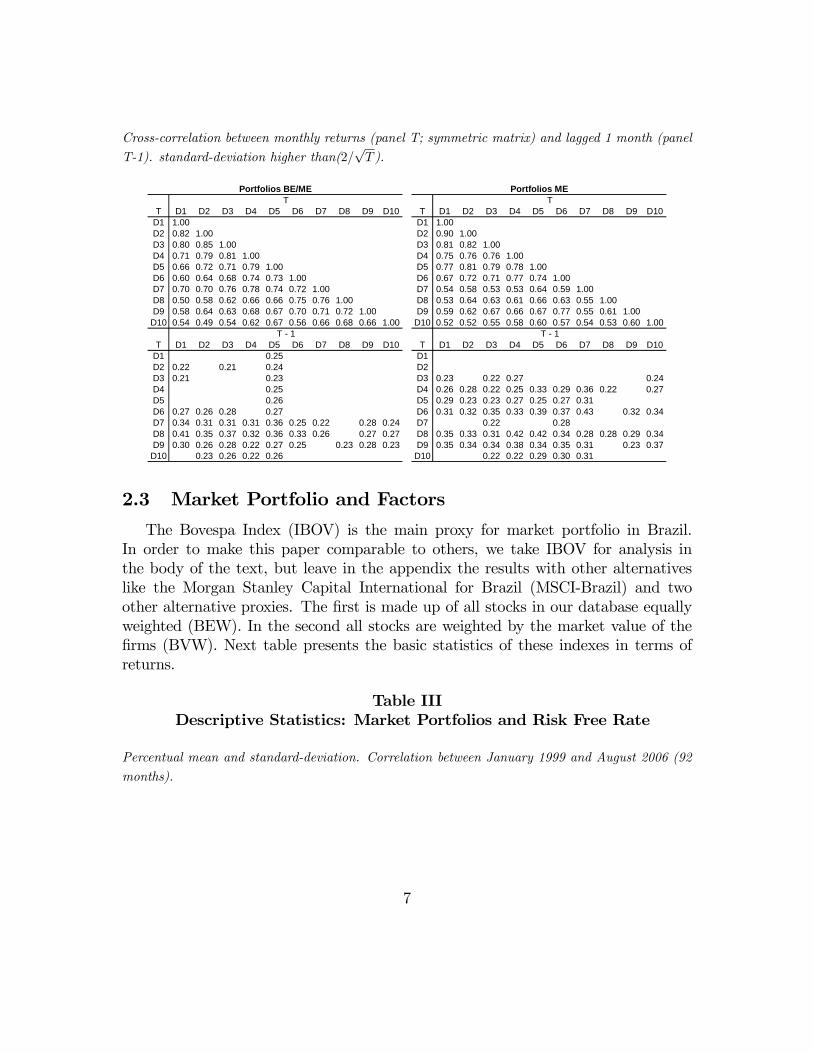
Cross-correlation between monthly returns (panel T; symmetric matrix) and lagged 1 month (panel

T-1). standard-deviation higher than(2/√T ).

T D1 D2 D3 D4 D5 D6 D7 D8 D9 D10 T D1 D2 D3 D4 D5 D6 D7 D8 D9 D10D1 1.00 D1 1.00D2 0.82 1.00 D2 0.90 1.00D3 0.80 0.85 1.00 D3 0.81 0.82 1.00D4 0.71 0.79 0.81 1.00 D4 0.75 0.76 0.76 1.00D5 0.66 0.72 0.71 0.79 1.00 D5 0.77 0.81 0.79 0.78 1.00D6 0.60 0.64 0.68 0.74 0.73 1.00 D6 0.67 0.72 0.71 0.77 0.74 1.00D7 0.70 0.70 0.76 0.78 0.74 0.72 1.00 D7 0.54 0.58 0.53 0.53 0.64 0.59 1.00D8 0.50 0.58 0.62 0.66 0.66 0.75 0.76 1.00 D8 0.53 0.64 0.63 0.61 0.66 0.63 0.55 1.00D9 0.58 0.64 0.63 0.68 0.67 0.70 0.71 0.72 1.00 D9 0.59 0.62 0.67 0.66 0.67 0.77 0.55 0.61 1.00D10 0.54 0.49 0.54 0.62 0.67 0.56 0.66 0.68 0.66 1.00 D10 0.52 0.52 0.55 0.58 0.60 0.57 0.54 0.53 0.60 1.00

T D1 D2 D3 D4 D5 D6 D7 D8 D9 D10 T D1 D2 D3 D4 D5 D6 D7 D8 D9 D10D1 0.25 D1D2 0.22 0.21 0.24 D2D3 0.21 0.23 D3 0.23 0.22 0.27 0.24D4 0.25 D4 0.26 0.28 0.22 0.25 0.33 0.29 0.36 0.22 0.27D5 0.26 D5 0.29 0.23 0.23 0.27 0.25 0.27 0.31D6 0.27 0.26 0.28 0.27 D6 0.31 0.32 0.35 0.33 0.39 0.37 0.43 0.32 0.34D7 0.34 0.31 0.31 0.31 0.36 0.25 0.22 0.28 0.24 D7 0.22 0.28D8 0.41 0.35 0.37 0.32 0.36 0.33 0.26 0.27 0.27 D8 0.35 0.33 0.31 0.42 0.42 0.34 0.28 0.28 0.29 0.34D9 0.30 0.26 0.28 0.22 0.27 0.25 0.23 0.28 0.23 D9 0.35 0.34 0.34 0.38 0.34 0.35 0.31 0.23 0.37D10 0.23 0.26 0.22 0.26 D10 0.22 0.22 0.29 0.30 0.31

Portfolios BE/MET

T - 1

Portfolios MET

T - 1

2.3 Market Portfolio and Factors

The Bovespa Index (IBOV) is the main proxy for market portfolio in Brazil.In order to make this paper comparable to others, we take IBOV for analysis inthe body of the text, but leave in the appendix the results with other alternativeslike the Morgan Stanley Capital International for Brazil (MSCI-Brazil) and twoother alternative proxies. The first is made up of all stocks in our database equallyweighted (BEW). In the second all stocks are weighted by the market value of thefirms (BVW). Next table presents the basic statistics of these indexes in terms ofreturns.

Table IIIDescriptive Statistics: Market Portfolios and Risk Free Rate

Percentual mean and standard-deviation. Correlation between January 1999 and August 2006 (92

months).

7

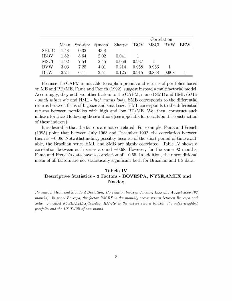
CorrelationMean Std-dev t(mean) Sharpe IBOV MSCI BVW BEW

SELIC 1.48 0.32 43.8IBOV 1.82 8.64 2.02 0.041 1MSCI 1.92 7.54 2.45 0.059 0.937 1BVW 3.03 7.25 4.01 0.214 0.958 0.966 1BEW 2.24 6.11 3.51 0.125 0.915 0.838 0.908 1

Because the CAPM is not able to explain premia and returns of portfolios basedon ME and BE/ME, Fama and French (1992) suggest instead a multifactorial model.Accordingly, they add two other factors to the CAPM, named SMB and HML (SMB- small minus big and HML - high minus low). SMB corresponds to the differentialreturns between firms of big size and small size. HML corresponds to the differentialreturns between portfolios with high and low BE/ME. We, then, construct suchindexes for Brazil following these authors (see appendix for details on the constructionof these indexes).It is desirable that the factors are not correlated. For example, Fama and French

(1995) point that between July 1963 and December 1992, the correlation betweenthem is −0.08. Notwithstanding, possibly because of the short period of time avail-able, the Brazilian series HML and SMB are highly correlated. Table IV shows acorrelation between such series around −0.68. However, for the same 92 months,Fama and French’s data have a correlation of −0.55. In addition, the unconditionalmean of all factors are not statistically significant both for Brazilian and US data.

Tabela IVDescriptive Statistics - 3 Factors - BOVESPA, NYSE,AMEX and

Nasdaq

Percentual Mean and Standard-Deviation. Correlation between January 1999 and August 2006 (92

months). In panel Bovespa, the factor RM-RF is the monthly excess return between Ibovespa and

Selic. In panel NYSE/AMEX/Nasdaq, RM-RF is the excess return between the value-weighted

portfolio and the US T-Bill of one month.

8

CorrelationMean Std.-dev. t(M) RM-RF SMB HML

BOVESPARM −RF 0.35 8.55 0.39 1SMB 0.99 6.38 1.49 −0.40 1HML −0.79 8.74 −0.87 0.08 −0.68 1

NYSE/AMEX/NASDAQRM −RF 0.06 4.51 0.12 1SMB 0.57 4.58 1.18 0.26 1HML 0.60 4.22 1.37 −0.52 −0.55 1

3 Theory and Econometric Tests

The main prediction of the CAPM is that the expected return of a portfoliofollows a linear relationship with its β:

E [Ri,t −Rf,t] = λmβi (1)

for every t = 1, 2, . . . , T , whereλm is the risk price or risk premium given by E [Rm,t −Rf,t] ;Rm,t is the return of the market portfolio at time t; andβi is the amount of risk in portfolio i.The coefficient βi may be estimated by ordinary least squares according to the

following equation:

Ri,t −Rf,t = αi + βi (Rm,t −Rf,t) + εi,t (2)

for every i = 1, 2, . . . , N .The CAPM theory generates three main implications that may be tested, accord-

ing to Campbell, Lo and MacKinlay (1997):

1. The intercept is zero in equation (2);

2. The risk premium is positive λm > 0;

3. There is a linear relationship between βs and expected return, following equa-tion (1).

As a matter of fact, the empirical evidence regarding the US rejected the theory.Blume and Friend (1975) and Black, Jensen and Scholes (1972) report an intercept

9

different from zero, specially in the post-War period. Fama and MacBeth (1973)10

confirmed their results, although they have not rejected the other two implicationsof equation (1).In order to take into account some of these stylized facts, Black (1972) relaxes

the assumption about the existence of a risk free asset and introduces the zero-betaportfolio, which is a minimum variance portfolio uncorrelated with the market port-folio. On the other hand, Roll (1977) criticizes the proxy for the market portfolio byarguing that it contains only observed asset returns, rather than representing the re-turns of the entire economy. The market portfolio, hence, would not be observable,because any possible proxy one can think of cannot consider intangible assets forexample, therefore the theory is not testable. In view of this situation, Ross (1976)proposes another model, named arbitrage pricing theory (APT), with assumptionsless restrictive than the CAPM11. In fact, by resuming portfolio choices to choicesover mean-and-variances, the CAPM implicitly assumes a direct relationship betweenwealth and consumption, which is a very restrictive hypothesis considering there is atemporal dynamics between these variables. As a consequence, Merton (1973) intro-duces an intertemporal asset pricing model, heavily criticizing the static assumptionof the CAPM. The models of Lucas (1978) and Breeden (1979) follow that line ofrepresentative agents and formulate the consumption CAPM theory, also known asCCAPM. In those models, the decisions about where allocating wealth result froman intertemporal maximization of the utility function, where the consumption is thecontrolled variable and the financial markets enters in order to smooth consumptionover time.Parallel to the theoretical development described, new empirical evidence came

out, heavily questioning the CAPM. In particular, assets grouped together accordingthe financial characteristics of firms as size, book value and dividends presented re-turns unexplained by β (Basu (1977), Banz (1981) and Rosenberg, Reid and Lanstein(1985)).Such an evidence has motivated Fama and French (1992, 1993) to estimate a

10In that work, the authors introduce as estimation methodoloy known as 2-stage Fama andMacBeth methodoloy. The portfolios are ordered according to the βs magnitude, in order to reducedispersion, which would make insignificant parameter λm. Thus, in the first stage, one estimatesby OLS each β using time series data. In the second stage, the estimated βs become explanatoryvariables of the mean returns of the portfolios at each time t. The total risk premium is thenobtained by averaging the risk premia of each time OLS estimation of λm, and the standard-deviation is calculated accordingly.11For instance, the CAPM demands homogeneous agents with quadratic preferences or multi-

variate normality of returns (as in Markowitz (1952)), and an efficient market portfolio. The APTassumes non arbitrage and a considerable number of assets.

10

multifactorial model by including some ad hoc factors taylored to capturate observedanomalies. Thus the expected excess return between the portfolio (Ri) and the riskfree rate (Rf) responds to three factors: the excess return of the market portfolio,the return spread between portfolios with big and small firms, SMB, and the returnspread between firms with high and low BE/ME, HML:

E [Ri,t −Rf,t] = λmβi + λssi + λhhi (3)

where λi, i = m, s, h, are the expected premia, respectively measured byE [Rm −Rf ],E [SMB] and E [HML]. The coefficients (βi, si, hi) measure the portfolio i sensitiv-ity to each factor and are obtained through the time series regression:

Ri,t −R,f,t = ai + βi (Rm,t −Rf,t) + siSMBt + hiHMLt + εt,i (4)

In equilibrium, agents require that premium to offset the risk of owning suchassets. Fama e French do not provide a theory based of primitive foundations tojustify why using exactly those factors. However, Fama e French (1996) argue thatfirms with profits sistematically low are facing financial difficulties tend to have ahigh BE/ME. Given those additional risks, returns must be higher in equilibrium. Bycontrast, consolidaded firms have low BE/ME, hence a low return, independently ofother risks. Similarly, the market value of a firm indicates a negative financial statusor mirrors a natural risk of an incipient firm. In such case, returns ex-ante mustreflect such additional risks.This paper tests the implication of the CAPM and the three factors model of

Fama and French, hecenforth FF, for Brazil and the US. The tests focus on twobasic implications of the models:

1. The intercepts are jointly null for all assets in the time series regressions rep-resented by equations 2 and 4;

2. The cross-section adjustment between the expected return predicted by themodel and the observed mean return, according to equations 1 e 3.

A by-product of the procedure is to estimate the risk premium for Brazil, spreadlyused by market practitioners for evaluating cash flows of corporations. However, wedo not test formally another possible implication regarding whether the risk premiumis the expected excess return, λm = E (Rm,t −Rf).

11

3.1 Test of Intercepts

By assumption, the multifactorial model is able to capturate the behavior ofreturns. Such an implication will be true if the intercepts are all null. A usual testfor that implication was suggested by Gibbons, Ross and Shanken (1989). However,the test does not adjust for autocorrelated series, which is a feature often foundin financial series. Alternatively, one may use the test by MacKinlay e Richardson(1991), based on the overidentification test using GMM estimation method.In this work, we perform and compare both alternatives. Therefore, let us de-

scribe each one in what follows.

3.1.1 Gibbons, Ross e Shanken’s (1989) Test

Using the OLS estimates of equation 4, one can test the null hypothesis thatαi = 0 ∀ i. If the disturbances are temporally independent and jointly normal, withmean zero, Gibbons, Ross and Shanken (1989) suggest using the following statistics:

GRS =

µT

N

¶µT −N −K

T −K − 1

¶"a0Σ−1a

1 + μ0f Σ−1f μf

#∼ F (N, T −N −K) (5)

wherea is an N × 1 vector of constants estimated by either equation 2 or 4;Σ is an N ×N residual covariance matrix;μf is a K × 1 factors means12; andΣf is a K ×K factor covariance matrix.

3.1.2 Overidentification Test

An advantage of the GMM estimation over the OLS model (used in the GRS test)is that GMM does not assume any hypothesis over the distribution of the series likei.i.d.(serial uncorrelatedness and homoskedasticity). However, in general, financialseries do present at least autocorrelation. Therefore, MacKinlay and Richardson(1991) suggest two tests through GMM to overcome the difficulties of the GRS test.The first test consists of estimating (α,β0)0 by GMM and testing the null hypothesisthat αi = 0, ∀ i, where β0 is the vector of factor coefficients.The second test consists of imposing αi = 0, ∀ i, estimating the model by GMM,

and then testing whether the objective function at the minimum is statistically null.

12K = 1 in the CAPM model and K = 3 in the FF model.

12

That is, use a vector of ones as instrument, and, if the null is false, the objectivefunction will fail in being statistically zero. We perform this second test in this work.Therefore, let ri,t = Ri,t−Rf,t, and define the population moments in the following

way:

E [g (wt,β0)] = E

∙rt − β00ft

(rt − β00ft)⊗ ft

¸=

∙00

¸(6)

wherert = [r1,t, r2,t . . . , rN,t]

0 is an N × 1 vector of excess returns;ft is a K × 1 vector of factors;⊗ is the Kronecker operator.By assumption data is ergodic, therefore the population moments have a sample

analog given by:

gT (w,β) = T−1TXt=1

g (wt,β) ,

where wt is a vector of observed variables.The GMM estimator gives us β

gmm= arg

βmin {QT (β)}, from:

QT (β) = gT (w,β)0WTgT (w,β) , (7)

whereWT is a matrix that weights efficiently each moment.There are more moments than parameters to be estimated. It is necessary to

estimate NK coefficients (N portfolios and K parameters in each), and there areN (K + 1) moment conditions, every portfolio is multiplied by the factor plus theconditions that the errors are zero in each portfolio. Hence, the model is overidentifiedand, as such, the quantity QT

³βgmm

´follows a χ2 distribution with N degrees of

freedom (Hansen (1982)). Consequently, it can be statistically tested. If we fail toreject the null that all moments are statistically zero, then the model is correctlyidentified and, consequently the intercepts are statistically jointly null.

3.2 Risk Premium

The popularity of the CAPM and FF models probably resides in the fact thatthey establish a straightforward relationship of return differentials through the pric-ing equations (1) and (3). A natural way of testing the models emerges from the

13

coefficients significance and sign of the cross-sectional pricing equation between ex-cess returns and βs.However, since the βs are estimated in the first step, it is needed to adjust the

variance of the estimated parameters, λs, in the second step. That’s why Fama andMacBeth (1973) suggested the OLS estimation in two stages. However, nowadaysthere are other techniques which make Fama and MacBeth’s procedure obsolete.They are the GMM and the ITNLSUR.Importantly, Shanken and Zhou (2007) recently have studied the small sample

properties of cross-sectional expected return estimators like GMM, Maximum Like-lihood, Fama and MacBeth’s (1973) procedure and some variants as the GeneralizedLeast Squeares - GLS - and the Weighted Least Squares - WLS . They concludethat all estimators are identical for samples greater than 960 observations (30 years).GMM performs as well as the other methods for N = 48 and T > 120. However,GMM gets worse when N = 25.Unfortunately, it seems that nobody has tested CAPM and the FF models using

the ITNLSUR, which is a method that nests both the GLS and the WLS procedures,with asymptotic properties potentially better than those estimators’.

3.2.1 ITNLSUR

Burmeister and McElroy (1988)? proposed a new econometric model to estimatethe cross-sectional expected returns. Their model focuses on the APT, but it can beused for testing the CAPM and the FF models. The method is an iterated nonlinearseemingly unrelated regression and meant to correct many problems related with thetwo stage methods (OLS, GLS, WLS). Among the defficiencies associated with theconventional methods are the unrobustness of the estimates under non normality,loss of estimation efficiency, non uniqueness of the second stage estimators due tothe need of grouping assets in portfolios and problems with statistical inference.This section presents briefly the model by Burmeister and McElroy (1988), in

order to make it clear how it works. Thus, consider a multifactorial model with Kfactors and N assets. The ITNLSUR methods allows one to estimate simultaneouslythe NK βs and the K λs, through the econometric model:

Ri,t − λ0,t =KXj=1

βij (λj + fj,t) + εi,t, (8)

where, in principle, λ0,t is observed and will stand for the risk free asset.Notice in the model that βij multiples both fj,t (conventional first stage) and

λj (conventional second stage) simultaneously. That’s the way that Burmeister and

14

McElroy (1988) nest all models into one.Also, it is assumed that

Et [εi,t] = 0;

Et [εi,tεj,s] =

½σij, t = s0, t 6= s

; and

Et [εi,t |fj,s ] = 0.

Observe that there is no assumption about the error distribution. And when theerrors are multivariate normal, then the estimator is a maximum likelihood estimator.Let ρi ≡ Ri,t − λ0,t be a T × 1 vector representing the temporal excess returns

and rewrite the model in the following way (8):

ρi = [λ0 ⊗ 1T + f ]βi + εi = X (λ)βi + εi for i = 1, ..., N,

whereλ is a K × 1 vector of risk premia, depending on the factor loading;βi is a K × 1 vetor of βs of factors;1T is a T × 1 vector of ones; andX (λ) is a T ×K matrix.Stacking the N equalities above, one gets:

ρ ≡

⎛⎜⎝ ρ1...ρN

⎞⎟⎠ =

⎡⎢⎣ X (λ) 0 · · · 0...

.... . .

...0 0 · · · X (λ)

⎤⎥⎦⎛⎜⎝ β1

...βN

⎞⎟⎠+⎛⎜⎝ ε1

...εN

⎞⎟⎠ .

Rewriting more compactly, one gets:

ρ = [IN ⊗X (λ)]β + ε, (9)

whereβ = [β01, β

02, . . . , β

0N ]0;

ε = [ε01, ε02, . . . , ε

0N ]0 ;

The estimation process involves several steps. Firstly, the parameter θ =³aij, βij

´,

where aij = βijλ, is obtained by OLS conventionally, following equation (8). Thenthe residuals are used to estimate the covariance matrix given by Σ = [T−1e0iej].

Then, the parameters³β,λ

´are obtained iteratively, by minimizing the quadratic

error of equation (9):

15

Q³λ,β; Σ

´= [ρ− [IN ⊗X (λ)]β]0

³Σ−1 ⊗ IN

´[ρ− [IN ⊗X (λ)]β] .

The process follows iteratively until covergence, using the estimated values³βs,λs´

to generate Σs and to minimize Q³λ, β; Σs

´. Notice that the process is not more

than quadratic residuals minimizations, which implies estimators strongly consistentand asymptotically normal, even when the errors are not normally distributed.

3.2.2 GMM

The ITNLSUR method assumes the errors are conditionally homokesdatic andserially uncorrelated. The GMM method relaxes those hypotheses and allows oneto analyse in detail some economic implications. The main advantage is doubtlessthe possibility of expressing the information available to the agents through themoment conditions in order to make decisions. As such, the number of momentsmay be greater than the number of parameters, which makes GMM overidentifiedand reflects the information set of agents.However, GMM has not been much used to estimate the cross-section returns

in equation (1). According to Shanken and Zhou (2007), the reason for that isthe difficulty in finding out numerical solutions for the problem, since there are alarge number of parameters to estimate coupled with the nonlinearity of the model.Therefore, if the problem can be linearized in some way and conveniently weighted,then those difficulties may be overcome.In line with this argument and following Harvey and Kirby (1995), Shanken and

Zhou (2007) suggest estimating the model sequentially. To see how it works, defineRt as the N × 1 vector of portfolios or assets to which corresponds an N × 1 vectorof means, μr, that is:

E (Rt) = μr.

Similarly, let f be a K × 1 vector of factor to which correspond another K × 1vector of factor means, μf :

E (ft) = μf .

Let Σf be a K ×K factor covariance matrix, such that:

Eh¡ft − μf

¢ ¡ft − μf

¢0i= Σf .

16

The matrix contains K(K+1)2

distinct covariances. To obtain a vector of thesecovariances, apply the VECH operator, which stacks the columns of the lower portionof a covariance matrix, such that:

E³vech

h¡ft − μf

¢ ¡ft − μf

¢0i´= vech (Σf) .

Now, it is necessary to obtain the covariance matrix between Rt and ft, whosedimension is N ×K. Such covariance is given by

Eh¡Rt − μf

¢ ¡ft − μf

¢0i= Σrf .

For ease of notation in what follows define¡Rt − μf

¢ ¡ft − μf

¢0 ≡ Σrft, suchthat E (Σrft) = Σrf . Then, the last N moment conditions requires that the cross-sectional errors are jointly zero, such that:

E¡Rt − γ01N −ΣrftΣ

−1f γk

¢= 0,

where γk is a K × 1 vector of parameters. If K = 1, then this could be the marketpremium, for example.Putting together all the moment conditions, one obtains:

E [g (wt,θ0)] = E

∙g1¡wt,θ

10

¢g2¡wt,θ

10,θ

20

¢ ¸ == E

⎡⎢⎢⎢⎣Rt − μrft − μf

vechh¡ft − μf

¢ ¡ft − μf

¢0 −Σf

iRt − γ01N −ΣrftΣ

−1f γk

⎤⎥⎥⎥⎦ =∙00

¸.

Notice the N × K matrix β ≡ ΣrfΣ−1f corresponds to the matrix of βs of the

first step of multifactorial model. In other words, it corresponds to the explanatoryvariables of the second step of Fama and MacBeth’s procedure. Hence, there areM = N+K+ K(K+1)

2+N moments and P = N +K+ K(K+1)

2+K+1 parameters to

estimate. The sequential estimation proposed by Shanken and Zhou (2007) proceedsin two steps. In the first step estimate the P1 = N+K(K+3)

2parameters using the first

N + K(K+3)2

moments, that is, obtain bθ1 = ∙bμ0r, bμ0f , vech³bΣf

´0¸0. Of course, in that

case the weighting matrix is W1T = IN+

K(K+3)2

. Then, use the estimated parameters

17

in the last set of moments to estimate the other P2 = K + 1 parameters, that is,obtain bθ2 = ¡bγ0,bγ0k¢0. The advantage of this procedure is that all the estimationsare linear, which makes it easier to find out the solutions.In the second step, there is overidentification, provided that N > P2, which is

true either for the CAPM or for the FF models. However, in this case, it is veryimportant how to choose the weighting matrix, W2T . Following Ogaki (1993) andgiven W1T is identity, Shanken and Zhou (2007) show that the optimal weightingmatrix in the second step is:

W2T =

∙¡−Γ21Γ−111 I

¢ST

µ−Γ21Γ−111

I

¶¸−1,

where Γ =∙Γ11 Γ12Γ21 Γ22

¸is anM×P corresponding to the derivative of the moments

with respect to the parameters and I a P2 × P2 identity matrix. Note that Γ11 is aP1 × P1 matrix and that Γ22 = [−1N − βN×K ] is an N × P2 matrix.For simplicity, but following Harvey and Kirby (1995), we assume that Γ21 = 0.

As pointed out by Shanken and Zhou (2007), this assumption implies that the factormodel disturbances have zero mean conditional on the factors.

4 Empirical Analyses

Empirical studies testing either the CAPM or FF models are scarce in Brasilcompared with the US literature. One of the possible reasons is the low amountof data, mainly because the long megainflationary period before 1994 distorted theavalaible data. Another possible reason is the low number of corporations with stockstraded, which makes the researchers disagree about which stocks taking into account.Given such a situation, we compare the results with US data by estimating the modelsusing the same period and firms grouping. The intention is to establish a dialoguewith the vast US literature, where the main results were extensively documented.By contrasting the results, we believe the conclusions would be more reliable.

4.1 Intercept Tests

This section tests whether the intercepts of equations (2) and (4) are jointly null,both for the Brazilian and the US samples, using portfolios based on the ME andBE/ME criteria.

18

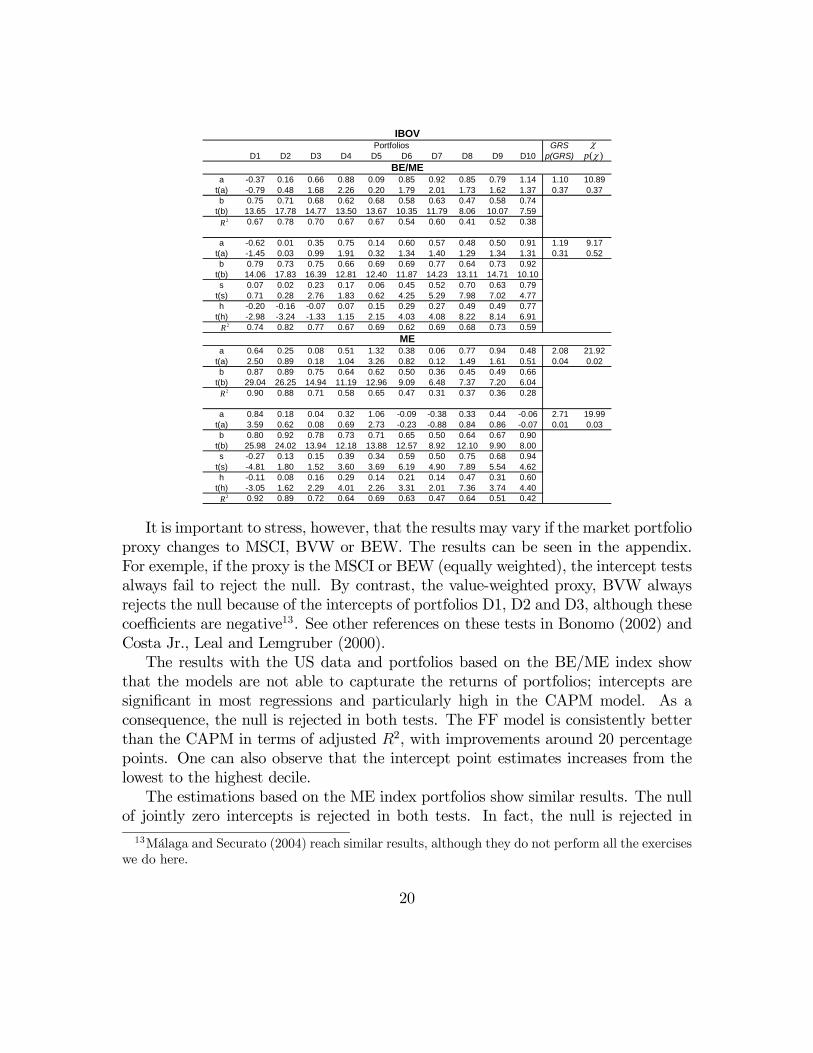
For the Brazilian data and portfolios based on the BE/ME criterium, the statisticsGRS and χ fail to reject the null of jointly intercepts equal to zero both in the CAPMand in the FFmodels. In the CAPMmodel, the intercepts are individually significantin portfolios D4 and D7 (5%) and D3, D6 and D8 (10%). However, by introducingthe SMB and HML factors, only D4’s intercept rejects the null at 10% of significance.In terms of adjusted R2, the FF model is marginally better than the CAPM, exceptin the upper extreme portfolios D8, D9 and D10 where the difference is clear.For the portfolios based on the ME criterium, the statistics GRS and χ reject the

null of jointly intercepts equal to zero in both CAPM and FF models. The rejectionis due to the non zero intercepts of portfolios D1 and D5. In this data set case, thedifference between models in terms of adjusted R2 is larger on portfolios D6 throughD10, where the FF models’ adjustment coefficients are higher.Although most of the intercepts are not significant across the portfolios, it is

possible to observe an increasing pattern in the point estimates from the lowest tothe highest BE/ME decile. Surprisingly is the fact of the βs being less than one inevery portfolio in both models.

Table VIntercept Tests and Time Series Regression of Portfolios BE/ME and

ME (BOVESPA)

The Estimated Equation is Ri,t − Rf,t = ai + bi (Rm,t −Rf,t) + siSMBt + hiHMLt + εt,i. t() is

the t-statistics of the OLS regressions. p(GRS) and p(χ) correspond to the p-values of the statistics

GRS and χ described in the last section. The Market Portfolio is the Ibovespa and Selic is the risk

free rate. Sample from January 1999 to August 2006 (92 months).

19

GRSD1 D2 D3 D4 D5 D6 D7 D8 D9 D10 p(GRS)

a -0.37 0.16 0.66 0.88 0.09 0.85 0.92 0.85 0.79 1.14 1.10 10.89t(a) -0.79 0.48 1.68 2.26 0.20 1.79 2.01 1.73 1.62 1.37 0.37 0.37b 0.75 0.71 0.68 0.62 0.68 0.58 0.63 0.47 0.58 0.74

t(b) 13.65 17.78 14.77 13.50 13.67 10.35 11.79 8.06 10.07 7.590.67 0.78 0.70 0.67 0.67 0.54 0.60 0.41 0.52 0.38

a -0.62 0.01 0.35 0.75 0.14 0.60 0.57 0.48 0.50 0.91 1.19 9.17t(a) -1.45 0.03 0.99 1.91 0.32 1.34 1.40 1.29 1.34 1.31 0.31 0.52b 0.79 0.73 0.75 0.66 0.69 0.69 0.77 0.64 0.73 0.92

t(b) 14.06 17.83 16.39 12.81 12.40 11.87 14.23 13.11 14.71 10.10s 0.07 0.02 0.23 0.17 0.06 0.45 0.52 0.70 0.63 0.79

t(s) 0.71 0.28 2.76 1.83 0.62 4.25 5.29 7.98 7.02 4.77h -0.20 -0.16 -0.07 0.07 0.15 0.29 0.27 0.49 0.49 0.77

t(h) -2.98 -3.24 -1.33 1.15 2.15 4.03 4.08 8.22 8.14 6.910.74 0.82 0.77 0.67 0.69 0.62 0.69 0.68 0.73 0.59

a 0.64 0.25 0.08 0.51 1.32 0.38 0.06 0.77 0.94 0.48 2.08 21.92t(a) 2.50 0.89 0.18 1.04 3.26 0.82 0.12 1.49 1.61 0.51 0.04 0.02b 0.87 0.89 0.75 0.64 0.62 0.50 0.36 0.45 0.49 0.66

t(b) 29.04 26.25 14.94 11.19 12.96 9.09 6.48 7.37 7.20 6.040.90 0.88 0.71 0.58 0.65 0.47 0.31 0.37 0.36 0.28

a 0.84 0.18 0.04 0.32 1.06 -0.09 -0.38 0.33 0.44 -0.06 2.71 19.99t(a) 3.59 0.62 0.08 0.69 2.73 -0.23 -0.88 0.84 0.86 -0.07 0.01 0.03b 0.80 0.92 0.78 0.73 0.71 0.65 0.50 0.64 0.67 0.90

t(b) 25.98 24.02 13.94 12.18 13.88 12.57 8.92 12.10 9.90 8.00s -0.27 0.13 0.15 0.39 0.34 0.59 0.50 0.75 0.68 0.94

t(s) -4.81 1.80 1.52 3.60 3.69 6.19 4.90 7.89 5.54 4.62h -0.11 0.08 0.16 0.29 0.14 0.21 0.14 0.47 0.31 0.60

t(h) -3.05 1.62 2.29 4.01 2.26 3.31 2.01 7.36 3.74 4.400.92 0.89 0.72 0.64 0.69 0.63 0.47 0.64 0.51 0.42

ME

IBOVPortfolios

BE/ME( )p χχ

2R

2R

2R

2R

It is important to stress, however, that the results may vary if the market portfolioproxy changes to MSCI, BVW or BEW. The results can be seen in the appendix.For exemple, if the proxy is the MSCI or BEW (equally weighted), the intercept testsalways fail to reject the null. By contrast, the value-weighted proxy, BVW alwaysrejects the null because of the intercepts of portfolios D1, D2 and D3, although thesecoefficients are negative13. See other references on these tests in Bonomo (2002) andCosta Jr., Leal and Lemgruber (2000).The results with the US data and portfolios based on the BE/ME index show

that the models are not able to capturate the returns of portfolios; intercepts aresignificant in most regressions and particularly high in the CAPM model. As aconsequence, the null is rejected in both tests. The FF model is consistently betterthan the CAPM in terms of adjusted R2, with improvements around 20 percentagepoints. One can also observe that the intercept point estimates increases from thelowest to the highest decile.The estimations based on the ME index portfolios show similar results. The null

of jointly zero intercepts is rejected in both tests. In fact, the null is rejected in13Málaga and Securato (2004) reach similar results, although they do not perform all the exercises

we do here.

20

the CAPM because of portfolios D4 and D10. If the model is the FF the model isnot rejected to 5% using the GMM test. The increasing pattern of intercepts’ pointestimates is also present in the CAPM model but not in the FF.Differently from the Brazilian case, the βs of the portfolios BE/ME and ME are

all greater than one in the CAPM model, but are less than 1 in portfolios D5-D10 ifestimation includes the HML and SMB factors.

Table VIIntercept Tests and Time Series Regression of Portfolios BE/ME and

ME (NYSE, AMEX and Nasdaq)

The Estimated Equation is Ri,t − Rf,t = ai + bi (Rm,t −Rf,t) + siSMBt + hiHMLt + εt,i. t() is


GRS and χ described in the last section. The Market Portfolio is the value-weighted and T-Bill is

the risk free rate. There are 92 monthly observations between January 1999 and August 2006.


a -0.23 0.48 0.64 0.82 1.02 1.29 1.24 1.24 1.45 1.76 4.19 37.90t(a) -0.40 1.16 1.85 2.58 3.29 4.23 3.96 3.85 3.93 3.74 0.00 0.00b 1.82 1.44 1.23 1.08 0.93 0.89 0.78 0.75 0.83 0.94

t(b) 13.90 15.20 15.59 15.09 13.24 12.88 11.03 10.28 9.96 8.850.68 0.72 0.73 0.71 0.66 0.64 0.57 0.54 0.52 0.46

a -0.17 0.12 0.16 0.28 0.43 0.70 0.59 0.57 0.76 1.00 4.64 29.29t(a) -0.42 0.38 0.62 1.20 2.01 3.51 2.89 2.90 3.02 2.73 0.00 0.00b 1.36 1.26 1.18 1.10 0.98 0.93 0.87 0.82 0.88 0.98

t(b) 13.14 16.42 18.10 18.72 18.28 18.28 16.78 16.39 13.89 10.55s 0.58 0.66 0.61 0.57 0.59 0.59 0.60 0.65 0.71 0.79

t(s) 5.59 8.64 9.41 9.72 11.00 11.76 11.72 13.10 11.23 8.66h -0.60 0.01 0.23 0.36 0.43 0.41 0.51 0.50 0.49 0.51

t(h) -4.79 0.08 2.95 4.98 6.58 6.64 8.05 8.19 6.30 4.530.85 0.86 0.86 0.86 0.85 0.86 0.83 0.84 0.80 0.70

a -0.22 0.29 0.34 0.56 0.28 0.31 0.29 0.53 0.65 1.34 2.81 27.66t(a) -1.02 1.43 1.61 2.40 1.04 0.95 0.81 1.39 1.40 2.54 0.00 0.00b 1.03 1.03 1.23 1.16 1.16 1.30 1.27 1.25 1.29 1.06

t(b) 21.31 22.49 25.57 22.00 18.91 17.75 15.54 14.39 12.39 8.850.83 0.85 0.88 0.84 0.80 0.78 0.73 0.69 0.63 0.46

a -0.14 0.17 0.12 0.30 0.00 -0.08 -0.29 -0.12 -0.04 0.85 2.66 16.30t(a) -0.84 0.88 0.57 1.31 -0.01 -0.30 -1.20 -0.49 -0.12 2.03 0.01 0.09b 1.15 1.14 1.31 1.23 1.19 1.25 1.25 1.22 1.21 0.89

t(b) 27.41 23.60 24.93 21.43 17.98 18.67 20.07 19.92 15.88 8.32s -0.26 -0.03 0.13 0.19 0.28 0.50 0.69 0.76 0.88 0.78

t(s) -6.27 -0.61 2.44 3.37 4.32 7.48 11.13 12.50 11.67 7.40h 0.10 0.22 0.24 0.25 0.21 0.18 0.33 0.37 0.31 0.09

t(h) 2.03 3.70 3.78 3.57 2.58 2.18 4.37 4.92 3.38 0.680.91 0.87 0.89 0.86 0.83 0.86 0.88 0.89 0.86 0.69

Portfolios

BE/ME

ME

VW

( )p χχ

2R

2R

2R

2R

21

4.2 Risk Premium

This section presents the estimates of equations (1) and (3) by GMM and ITNL-SUR methods. In the GMM case, the covariance function is estimated using theParzen weighting function following Andrews (1991), who argues it is preferable overthe Bartlett window, and, according to Ogaki (1993), it is computationally moreconvenient than the quadratic option.The choice of the bandwidth is more critical than the choice of the weighting

function (see Hall (2005)). For this reason, we estimate the model with 3 distinctbandwidths: none, 1 and 4. If the series are uncorrelated, then the bandwidth shouldbe zero. Hall (2005) suggests setting it equal to T

13 ' 4 because it minimizes the

mean square error of the covariance estimator. Finally, we also set the the bandwidthequal to 1 because the analysis of the series in Table II has shown that only first-lagcorrelations are statistically significant.The tables show the parameters estimated by GMM at the first stage, using the

identity as weighting matrix - GMM1 - and the inverse of the long run covariancematrix as weighting matrix, iterated until convergence - GMM IT. Monte Carlosimulations show that when the sample is small, GMM estimates are better if theobjective function is iterated until convergence (Ogaki (1993)). The argument forpresenting GMM1 is as follows. When one groups portfolios according to financialcharacteristics, the weights are the same for every asset. If the weighting matrixis optimal, the economic content of the covariance matrix is lost (see Yogo, 2006,Cochrane, 2005). Therefore, by comparing the parameters of the GMM1 we are ableto compare results from distinct, economic based, specifications. On the other hand,estimates obtained in GMM IT have nicer statistic properties. The estimates basedon the identity weighting matrix and one iteration are similar to those obtained byOLS. The estimates based on the identity weighting matrix itered until convergenceare similar to those obtained by GLS14.The portfolios used in the estimations are those defined by the BE/ME and

ME criteria. Moreover, we repeat the exercise using 44 stocks without any kind ofgrouping (44IBOV). In doing that, we avoid the criticism of Lewellen, Nagel andShanken (2006). They argue that the the βs are correlated with the other indexes.Before going on, one should choose to include or not a constant, λ0, in the model

(1) and (3) (λ0 stands for the exceptional return beyond the excess return of the assetwith respect to the risk free rate). This turned out to be crucial in our estimates sinceit changed sensitively the results. Such a phenomenum is also present in the US data

14The estimate in two stages by OLS, GLS and WLS as suggested by Shanken and Zhou (2007)are available under request.

22

and is often disregarded in studies. As a matter of fact, Lewellen, Nagel e Shanken(2006) show that recent successful articles in explaining the cross-sectional variabilityof returns, such as Lettau and Ludvigson (2001) and Yogo (2006), present hugeestimates for λ0, contradicting theory. Following economic arguments, we impose theintercept to be null; the appendix presents the estimation under the less restrictivespecification for portfolios ME using Brazilian data. As can be seen, the inclusion ofthe constant lead to negative risk premium and high positive intercepts estimates.Table VII presents the estimates for the 3 sets of portfolios (panels BE/ME, ME

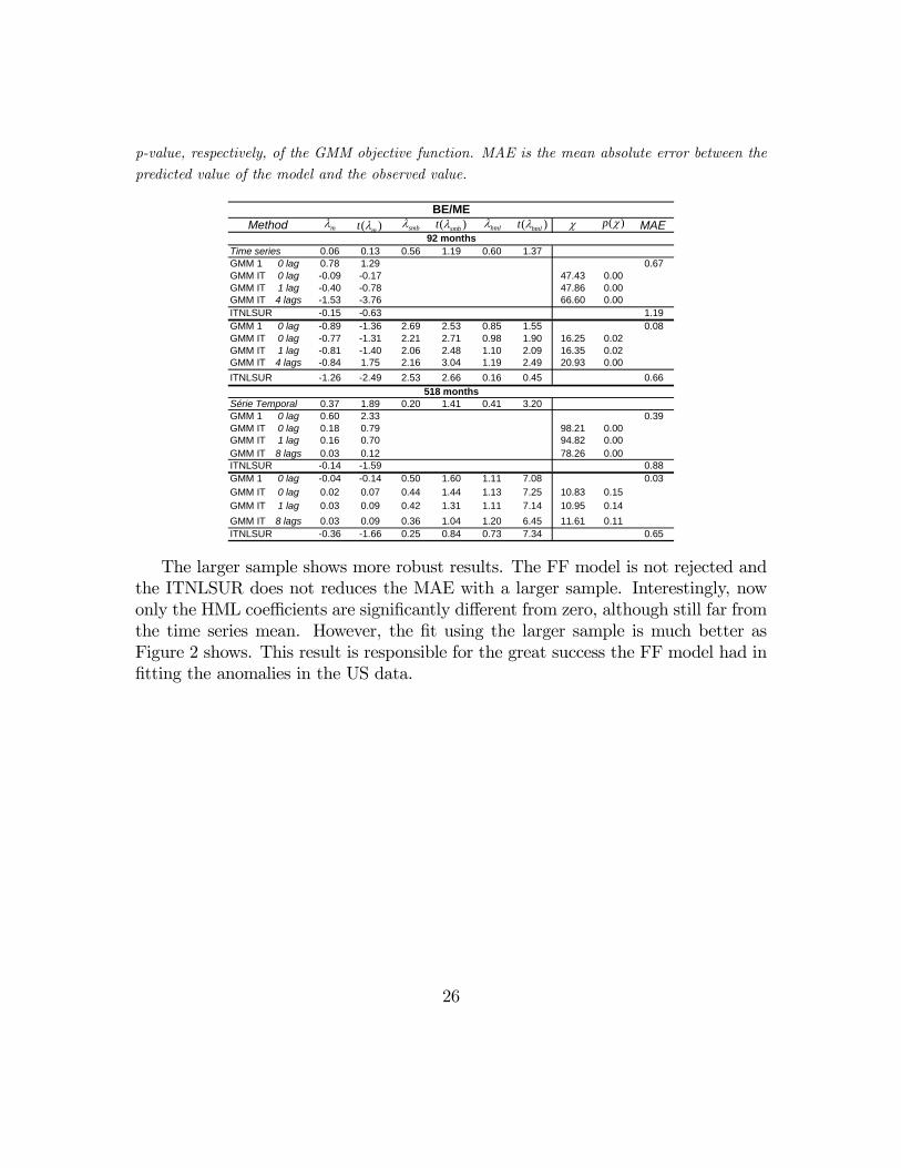
and 44IBOV) for Brazilian data. The CAPM model presented a positive market riskpremium for all variants, except in the case 44IBOV with 4 lags, where the modelfailed to converge. In the cases the coefficient was significantly different from zero(ITNLSUR for ME and 44IBOV portfolios), the market risk premium in annual termsis about 6.5% a very plausible and generally agreed figure in the private market.When the SMB and HML factors are included in the model, the risk premium is

still significant in the ITNLSUR method (ME and 44IBOV) at the same magnitude.Using the GMM method, the point estimates hardly resemble the time series means,possibly only on the ME portfolios. The estimates of the SMB premium, λsmb,approximates the time series mean around 0, 99% in the portfolios BE/ME accordingto the GMM method. The HML premium, λhml, is negative and approximates thetime series mean around −0, 79% in portfolios ME. However, GMM delivers nonsignificant coefficients and, in this sense, agree with time series means estimates.

Table VIICross-Sectional Regressions.

Econometric Model: E [Ri,t −Rf,t] = λmβi + λssi + λhhi. In the GMM1, WT = I. The weighting

covariance matrix is based on Parzen Spectral Density. The GMM IT model iterated until conver-

gence of the objective function. Bandwidth: 0, 1 and 4 lags. χ and p(χ) are the value and the

p-value, respectively, of the GMM objective function. MAE is the mean absolute error between the

predicted value of the model and the observed value. January 1999 to August 2006 (92 months).

23

MAETime Series 0.35 0.39 0.99 1.49 -0.79 -0.87

GMM 1 0 lag 1.23 1.22 0.43GMM IT 0 lag 1.15 1.18 10.90 0.28 0.45GMM IT 1 lag 1.09 1.07 10.88 0.28 0.46GMM IT 4 lags 0.98 0.96 13.01 0.16 0.49ITNLSUR 0.43 1.39 0.63GMM 1 0 lag 0.53 0.53 1.05 0.44 0.19 0.10 0.22GMM IT 0 lag 0.47 0.47 1.07 0.82 0.12 0.08 6.45 0.49 0.22GMM IT 1 lag 0.60 0.58 1.03 0.80 0.14 0.10 6.19 0.52 0.22GMM IT 4 lags 1.31 1.25 0.73 0.61 0.34 0.26 6.02 0.54 0.50ITNLSUR 0.04 0.10 0.39 0.33 0.66 0.57 0.51

GMM 1 0 lag 1.15 1.14 0.32GMM IT 0 lag 1.46 1.51 17.74 0.04 0.41GMM IT 1 lag 1.25 1.28 17.20 0.05 0.34GMM IT 4 lags 0.55 0.60 19.85 0.02 0.43ITNLSUR 0.56 2.77 0.43GMM 1 0 lag 0.96 1.02 0.44 0.41 -0.58 -0.29 0.32GMM IT 0 lag 0.93 1.00 0.17 0.17 -0.45 -0.25 15.39 0.03 0.31GMM IT 1 lag 0.84 0.89 0.19 0.18 -0.62 -0.33 15.09 0.03 0.34GMM IT 4 lags 0.43 0.46 0.58 0.64 -1.25 -0.74 18.39 0.01 0.51ITNLSUR 0.62 2.86 -0.54 -0.70 -0.21 -0.14 0.59

GMM 1 0 lag 0.86 0.90 1.15GMM IT 0 lag 1.26 1.38 77.37 0.00 1.17GMM IT 1 lag 1.09 1.22 84.53 0.00 1.15GMM IT 4 lags -1.98 -4.88 569.61 0.00 2.75ITNLSUR 0.51 5.13 1.20GMM 1 0 lag 0.94 1.01 -1.28 -1.32 -0.73 -0.61 1.12GMM IT 0 lag 0.87 0.95 0.40 0.50 -1.76 -1.65 69.16 0.00 1.68GMM IT 1 lag 0.74 0.82 0.21 0.28 -1.45 -1.39 77.42 0.00 1.54GMM IT 4 lags -1.10 -2.41 2.25 6.31 -1.40 -2.67 516.68 0.00 2.38ITNLSUR 0.56 5.30 -0.30 -0.66 -1.52 -2.78 1.04

44IBOV

Method

BE/ME

ME

χ ( )p χ( )mt λmλ ( )smbt λsmbλ ( )hmlt λhmlλ

When comparing both models in terms of mean absolute error (MAE), the great-est improvement occurs in the BE/ME portfolios, where the error is reduced from0.43% with the CAPM especification to 0.22% with FF. There is only a tiny im-provement in the 44IBOV portfolios, decreasing from 1.15% to 1.12%, although thereduction is greater in the ITNLSUR estimation.In the ME portfolios, both the CAPM and the FFmodels had similar performance

in terms of MAE. Figure 1 plots GMM1 estimates versus actual time series meansfor the indexes portfolios, and ITNLSUR estimates for the 44IBOV data set. Inany case, the χ statistics has rejected the models as well specified, but that is not asurprise as we shall see with the US data.

24

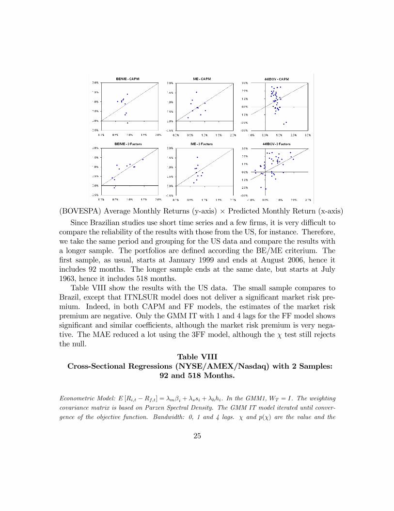
(BOVESPA) Average Monthly Returns (y-axis) × Predicted Monthly Return (x-axis)Since Brazilian studies use short time series and a few firms, it is very difficult to

compare the reliability of the results with those from the US, for instance. Therefore,we take the same period and grouping for the US data and compare the results witha longer sample. The portfolios are defined according the BE/ME criterium. Thefirst sample, as usual, starts at January 1999 and ends at August 2006, hence itincludes 92 months. The longer sample ends at the same date, but starts at July1963, hence it includes 518 months.Table VIII show the results with the US data. The small sample compares to

Brazil, except that ITNLSUR model does not deliver a significant market risk pre-mium. Indeed, in both CAPM and FF models, the estimates of the market riskpremium are negative. Only the GMM IT with 1 and 4 lags for the FF model showssignificant and similar coefficients, although the market risk premium is very nega-tive. The MAE reduced a lot using the 3FF model, although the χ test still rejectsthe null.

Table VIIICross-Sectional Regressions (NYSE/AMEX/Nasdaq) with 2 Samples:

92 and 518 Months.




25


predicted value of the model and the observed value.

MAE

Time series 0.06 0.13 0.56 1.19 0.60 1.37GMM 1 0 lag 0.78 1.29 0.67GMM IT 0 lag -0.09 -0.17 47.43 0.00GMM IT 1 lag -0.40 -0.78 47.86 0.00GMM IT 4 lags -1.53 -3.76 66.60 0.00ITNLSUR -0.15 -0.63 1.19GMM 1 0 lag -0.89 -1.36 2.69 2.53 0.85 1.55 0.08GMM IT 0 lag -0.77 -1.31 2.21 2.71 0.98 1.90 16.25 0.02GMM IT 1 lag -0.81 -1.40 2.06 2.48 1.10 2.09 16.35 0.02GMM IT 4 lags -0.84 1.75 2.16 3.04 1.19 2.49 20.93 0.00ITNLSUR -1.26 -2.49 2.53 2.66 0.16 0.45 0.66

Série Temporal 0.37 1.89 0.20 1.41 0.41 3.20GMM 1 0 lag 0.60 2.33 0.39GMM IT 0 lag 0.18 0.79 98.21 0.00GMM IT 1 lag 0.16 0.70 94.82 0.00GMM IT 8 lags 0.03 0.12 78.26 0.00ITNLSUR -0.14 -1.59 0.88GMM 1 0 lag -0.04 -0.14 0.50 1.60 1.11 7.08 0.03GMM IT 0 lag 0.02 0.07 0.44 1.44 1.13 7.25 10.83 0.15GMM IT 1 lag 0.03 0.09 0.42 1.31 1.11 7.14 10.95 0.14GMM IT 8 lags 0.03 0.09 0.36 1.04 1.20 6.45 11.61 0.11ITNLSUR -0.36 -1.66 0.25 0.84 0.73 7.34 0.65

Method92 months

518 months

BE/MEχ ( )p χ( )mt λmλ ( )smbt λsmbλ ( )hmlt λhmlλ

The larger sample shows more robust results. The FF model is not rejected andthe ITNLSUR does not reduces the MAE with a larger sample. Interestingly, nowonly the HML coefficients are significantly different from zero, although still far fromthe time series mean. However, the fit using the larger sample is much better asFigure 2 shows. This result is responsible for the great success the FF model had infitting the anomalies in the US data.

26

(NYSE/AMEX/Nasdaq) Average Monthly Returns (y-axis) × Predicted Monthly Return (x-axis)

5 Conclusions

The intercept tests produce similar conclusions with respect to the CAPM andthe 3 Factors Fama-French models. When the market portfolio proxy is the Ibovespafor Brazil, the intercepts with portfolios selected according to the BE/ME criteriumare jointly null in both models, whereas under the ME criterium, the models are bothrejected. However, other proxies for the market portfolio may change the results. Ifthe proxies is either the MSCI Brazil or a portfolios with equal weights for the assets,then the models are not rejected at all.Notwithstanding, the point estimates increases from the lowest to the highest

portfolios as in the US case when portfolios selected according to the BE/ME cri-terium. Such an observation is independent of the proxy for the market portfolio.Possibly this reflects the presence of a value-premium in the Brazilian data, as thedescriptive statistics already showed. The phenomenum does not occur to portfolioschosen by the ME criterium.The cross-section regressions reflect this value premium; the inclusion of the two

additional factors in the Fama-French model improves explanatory power over the

27

CAPM model on the BE/ME portfolios: mean absolute error - MAE - falls from0.43% to 0.22% per month. On the other hand, both models perform similarly onthe ME portfolios, around 0.32% of monthly MAE. In the case of the 44IBOV dataset, the multifactorial model is marginally superior to the CAPM (1.15% to 1.12%).The US data are more conclusive, and justifies the success of the 3 factor model

relatively to the CAPM (MAE from 0.67% to 0.08% in the BE/ME portfolios). WithUS data, anomalies are sharper than Brazilian data, what really makes the CAPMperformance in the US to be unsatisfactory. Indeed, in the more robust resultswith the larger sample, the 3 Factor model was not rejected whereas the CAPMwas. In the reduced sample, the same qualitative conclusion is reached, although thesignificance of the parameters worsens.The risk premium, in general, was not statistically significant with Brazilian

data. However, when the premium was significant, it was positive; the ITNLSURpoint estimate indicates a premium of 6.5% per year, in line with private marketusually agreed expectations, whereas the time series mean pointed to 4.25% peryear although not statiscally significant. The factor premia SMB and HML wereboth statistically non significant, even when accounting for serial correlation. Usingthe US data, the premia SMB and HML were significants with the small and largesamples, respectively, and the market premia was zero.This paper aimed to contribute to the Brazilian empirical asset-pricing litera-

ture. Firstly, by comparing the performance of two of the most studied asset pricingmodels, the CAPM and Factors Fama-French models, using Brazilian data, under avariety of data sets. As we have seen, the success of the multifactorial model overthe CAPM in the US data is not matched in the Brazilian data. Despite findingevidence of a value-premium anomaly, the size anomaly is not as sharp as in the USdata in the 92 month period. On the other hand, we found that the reduced size ofour sample may have limited the robustness of the results. In fact, the FF model isrejected by the χ statistic in the short sample but not in the large sample. Secondly,two econometric methods were compared: GMM e ITNLSUR. We found the choiceof the econometric tool to be important. In particular, we were able measure theBrazilian risk premium to be positive and significative using the ITNLSUR method.To the best of our knowledge nobody had reached to the same result before. Thatviabilizes the use of domestic data to calculate such a premium. Importantly theresults come from ungrouped assets, hence the arbitraryness of chosing the portfoliosis mitigated.

28

6 References

7 Bibliografia

Andrews, D. W. K. (1991): “Heteroskedasticity and Autocorrelation ConsistentCovariance Matrix Estimation,” Econometrica, 59(3), 817—858.

Banz, R. W. (1981): “The Relationship between Return and the Market Value ofCommon Stocks,” Journal of Financial and Quantitative Analysis, 14, 421—441.

BASU, S. (1977): “Investment Performance of Common Stocks in Relation to theirPrice-Earnings Ratios: A Test of the Efficient Market Hypothesis,” Journal ofFinance, 32, 663—682.

Black, F. (1972): “Capital Market Equilibrium with Restricted Borrowing,” Jour-nal of Business, 75(3), 444—455.

Black, F., M. Jensen, and M. Scholes (1972): “The Capital Asset PricingModel: Some Empirical Tests,” in Studies in the Theory of Capital Markets, ed.by M. C. Jensen, pp. 79—121. Praeger, New York.

Blume, M., and I. Friend (1975): “The Asset Structure of Individual Portfolioswith Some Implications for Utility Functions,” Journal of Finance, 30, 585—604.

Bonomo, M. (2002): Financas Aplicadas Ao Brasil. Editora FGV, RJ.

Breeden, D. T. (1979): “An Intertemporal Asset Pricing Model with StochasticConsumption and Investment Opportunities,” Journal of Financial Economics, 7,265—296.

Burmeister, E., and M. B. McElroy (1988): “Arbitrage Pricing Theory as aRestricted Nonlinear Multivariate Regression Model,” Journal of Business andEconomic Statistics, 6(1), 29—42.

Campbell, J. Y., A. Lo, and C. MacKinlay (1997): The Econometrics of Fi-nancial Markets. Princeton University Press, Princeton.

COSTA Jr., Newton, R. L., and E. Lemgruber (2000): Mercado de Capitais:Analise Empirica No Brasil. Editora Atlas, SP.

Fama, E. F., and K. R. French (1992): “The Cross-Section of Expected StockReturns,” Journal of Finance, 47(2), 427—465.

29

(1993): “Common risk factors in the returns on stocks and bonds,” Journalof Financial Economics, 33, 3—56.

(1995): “Size and Book-to-Market Factors in Earnings and Returns,” Jour-nal of Finance, 50, 131—156.

(1996): “Multifactor Explanations of Asset Pricing Anomalies,” Journal ofFinance, 51(1), 55—84.

Fama, E. F., and J. MacBeth (1973): “Risk, Return and Equilibrium: EmpiricalTests,” Journal of Political Economy, 81, 607—636.

Gibbons, M. R., S. A. Ross, and J. Shanken (1989): “A Test of the Efficiencyof a Given Portfolio,” Econometrica, 57(5), 1121—1152.

Hall, A. R. (2005): Generalized Method of Moments. Oxford University Press, NewYork, NY.

Hansen, L. P. (1982): “Large Sample Properties of GeneralizedMethod of MomentsEstimators,” Econometrica, 50(4), 1029—1054.

Harvey, C., and C. Kirby (1995): “Analytic Tests of Factor Pricing Models,”Working Paper.

Lewellen, Jonathan, S. N., and J. Shanken (2006): “A Skeptical Appraisalof Asset-Pricing Tests,” NBER Working Paper.

Lintner, J. (1965): “The Valuation of Risky Assets and the Selection of RiskyInvestments in Stock Portfolios and Capital Budgets,” Review of Economics andStatistics, 47, 13—37.

Lucas, Jr., R. E. (1978): “Asset Prices in an Exchange Economy,” Econometrica,46, 1426—14.

MacKinlay, A. C., and M. P. Richardson (1991): “Using Generalized Methodof Moments to Test Mean-Variance Efficiency,” Journal of Finance, 46(2), 511—27.

Malaga, F. K., and J. R. Securato (2004): “Aplicação Do Modelo de TrêsFatores de Fama e French No Mercado Acionário Brasileiro - Um Estudo EmpíricoDo Período 1995-2003,” in EnAnpad. Anpad.

Markowitz, H. M. (1952): “Portfolio Selection,” Journal of Finance, 7(1), 77—91.

30

Merton, R. C. (1973): “An Intertemporal Capital Asset Pricing Model,” Econo-metrica, 41(5), 867—887.

Ogaki, M. (1993): Generalized Method of Moments: Econometric Applica-tionschap. 17, pp. 455—485, Handbook of Statistics, Vol 11. Elsevier Science Pub-lishers.

Roll, R. W. (1977): “A Critique of the Asset Pricing Theory’s Tests,” Journal ofFinancial Economics, 4, 129—176.

Rosenberg, B., K. Reid, and R. Lanstein (1985): “Persuasive evidence ofmarket inefficiency,” Journal of Portfolio Management, 11, 9—17.

Ross, S. A. (1976): “The Arbitrage Theory of Capital Asset Pricing,” Journal ofEconomic Theory, 13, 341—360.

Shanken, J., and G. Zhou (2007): “Estimating and Testing Beta Pricing Models:Alternative Methods and their Performance in Simulations,” Journal of FinancialEconomics, 84, 40—86.

Sharpe, W. F. (1964): “Capital Asset Prices: A Theory of Market EquilibriumUnder Conditions of Risk,” Journal of Finance, 19, 425—442.

Yogo, M. (2006): “A Consumption-Based Explanations of Expected Stock Re-turns,” Journal of Finance, 61(2), 539—580.

8 Appendix

The appedix division follows the body text. Details regarding each section followsthe text section titles.

8.1 Data Set and Portfolio Construction

8.1.1 Portfolios

Composition of ME Porftolios The firms were ordered according to theirmarke value (ME), and grouped in 10 portfolios (D1 the largest corporations, D10the smallest corporations). Firms with more than one stock were kept in the samegroup with the same weight. The returns were equally weighted. Next table presentsthe composition of the portfolios in 2006, based on information released in December2005.

31

Table A1Portfolios Composition ME in December 2005

The data set contains 123 firms, whose stocks were traded in Bovespa between January 1999 and

August 2006.

D1 D2 D3 D4 D5 D6 D7 D8 D9 D10PETR TNLP BRKM SBSP ACES GLOB AVPL RHDS FJTA IENGVALE TMAR BRTP SDIA LIGT LEVE PEFX BOBR IGBR INEPBBDC CMET GOAU GUAR DURA CNFB ITEC FBRA HGTX TELBAMBV EMBR VIVO NETC TMCP CLSC EBCO CRIV MTSA TRFOITAU CSNA EBTP BFIT PTIP PQUN ROMI FLCL TNCP TEKABBAS CMIG VCPA KLBN TMGC RSID BRIV BRGE VAGV MWETUBBR BESP BRTO PRGA ALPA MYPK FRAS ETER PNVL BCALITSA USIM TCSL SUZB CTNM COCE DXTG RPAD MNDL LIXCTLPP ARCZ LAME CGAS CESP CEPE ASTA LIPR PLAS ESTRELET TBLE CPSL FFTL UNIP ELEK PLTO EMAE MGEL SULTARCE CRUZ WEGE CEEB PMAM RIPI ILMD SGAS CGRA JBDUGGBR PCAR CPLE CBEE RAPT BSCT FESA PNOR BDLL MNPR

DPPI POMO MAGS

BE/ME The firms were ordered according to the size of the BE/ME index,from the lowest to the highest and grouped in 10 portfolios (D1 to D10). Firms withmore than one stock were kept in the same group with the same weight. We haveexcluded firms with negative book equity, they were grouped in portfolio VX. Nexttable shows the composition of the portfolios in 2006, based on information releasedin December 2005.

Tabela A2Portfolios Composition BE/ME in December 2005


August 2006.

VX D1 D2 D3 D4 D5 D6 D7 D8 D9 D10BCAL BSCT AMBV ARCZ ALPA ARCE BRKM AVPL ACES ASTA BDLLBOBR CMET BBDC BESP BBAS CNFB CEEB BRTO CEPE BRGE CESPESTR CPSL CGAS BFIT CBEE DURA COCE BRTP CGRA BRIV ELETMWET CRUZ EMBR CMIG CSNA DXTG LIGT CLSC CRIV CPLE EMAEPMAM GUAR FFTL ELEK GLOB GOAU POMO ETER CTNM EBCO FJTATEKA HGTX FRAS GGBR LIPR ILMD PQUN FBRA DPPI FESA IENGVAGV LAME ITAU ITSA MTSA ITEC ROMI IGBR EBTP JBDU INEP

MYPK LEVE PCAR PEFX KLBN TMAR PTIP FLCL PLTO LIXCNETC PRGA PETR RIPI TMCP USIM RHDS MAGS PNOR MGELRSID RAPT PLAS SDIA VIVO VCPA SUZB MNDL RPAD MNPRTBLE UBBR TLPP TCSL TRFO PNVL SBSP SULTVALE WEGE TNLP TMGC UNIP SGAS TNCP TELB

32

8.1.2 Factors

Fama and French - SMB and HML The 123 firms were split into twogroups: B (big) and S (small). The first group contained the 61 largest firms interms of market value, and the other, the remaining 62. The firms were again splitinto 3 groups according to the size of the index BE/ME: H (high), M (medium) andL (low). The extreme groups counted each for 30% of the firms, and the mediumgroup for 40% of the firms. The market value was calculated by multiplying the freefloat stocks times the price stocks.The intersection of these two groups makes 6 sets of stocks: HB, HS, MB, MS,

LB and LS, which weighted by the market value of each firm generate 6 portfolios.The composition of these stocks is rebalanced yearly on the basis of the Balancesheet corresponding to December of the previous year, except the initial portfoliobased on January 1999. Firms with negative equity were excluded. The next tableshows the last composition of firms in each group followed by a descriptive statistics.

Table A3Fama French Portfolios for SMB and HML in December 2005


August 2006.HB HS MB MS LB LS

ACES ASTA ALPA AVPL AMBV BSCTCESP BDLL ARCE CLSC ARCZ ELEKCPLE BRGE BBAS CNFB BBDC FRASCTNM BRIV BRKM COCE BESP HGTXEBTP CEPE BRTO DXTG BFIT LEVEELET CGRA BRTP ETER CGAS MYPKSBSP CRIV CBEE FBRA CMET PLAS

DPPI CEEB IGBR CMIG RSIDEBCO CSNA ILMD CPSLEMAE DURA ITEC CRUZFESA GLOB LIPR EMBRFJTA GOAU MTSA FFTLFLCL KLBN PEFX GGBRIENG LIGT PNVL GUARINEP PTIP POMO ITAUJBDU SDIA PQUN ITSALIXC SUZB RHDS LAME

MAGS TCSL RIPI NETCMGEL TMAR ROMI PCARMNDL TMCP TRFO PETRMNPR TMGC PRGAPLTO TNLP RAPTPNOR UNIP TBLERPAD USIM TLPPSGAS VCPA UBBRSULT VIVO VALETELB WEGETNCP

Table A4Descriptive Statistics - Fama French Six Portfolios: BOVESPA andNYSE/AMEX/Nasdaq between January 1999 and August 2006

33

Percentual Mean and Standard-Deviation. Market value (ME) in US$ million in December 2005

Portfolio returns equally weighted according to the market value.

Portfolios HB HS MB MS LB LSBOVESPA

Mean 2.02 3.63 3.49 3.12 2.76 4.48Std. dev. 11.52 7.18 8.99 7.20 7.32 11.61Mean ME 2, 534 122 8, 293 150 5, 808 281Firms 7 28 26 20 27 8

NYSE/AMEX/NASDAQMean 0.57 1.37 0.65 1.29 0.06 0.32Std. dev. 4.46 5.07 4.06 5.10 4.59 8.10Mean ME 11, 295 307 14, 090 463 16, 753 462Firms 174 935 311 1, 207 394 1, 213

The Brazilian portfolio mean returns present a pattern different from the USdata. Portfolios with low BE/ME (L) had a superior performance to portfolios withhigh BE/ME (H) given the size of the firm, against expected. On the other side,portfolios with small firms (S) had higher returns than big firms (B) given BE/ME,except in the medium range. In the US case, one can observe that small firms withhigh BE/ME had a superior mean return, as documented in the anomalies’ literature.In order to assess whether different aggregations of firms would result in different

results, we change slightly the usual procedure for constructing these series. In thefirst change, instead of weighting firms according to its size, we equally weight them(EW). And second, we keep the value-weighted procedure but we define new sections’thresholds for the BE/ME index: top 15%, 30%, 70% and 85% (bottom 15%). Withthis we expect to differenciate more the firms, getting the ones in the extreme side(VW15).The statistics for EW show that HB > LB and HS > LS, in line with the US

data. However, on the other side of the spectrum, only HS > HB, and slightly,while MB > MS and LB > LS. The statistics for VW15, also does not resemblethe US’ data, for instance we have H1S > L1S but H1B < L1B. On what followsand in the main part of the paper, we will adopt the standard procedure.

Table A5Descriptive Statistics - Fama French Six Portfolios Variations

Returns were equally weighted (EW) or according to market value (VW). The two extremes of 30%

of the BE/ME index were divided into two sections of 15% (VW15). Sample from January 1999 to

August 2006 (92 months).

34

BOVESPAEW HB HS MB MS LB LSMean 2.31 2.68 2.80 1.74 1.88 1.69Std. Dev. 9.74 6.52 7.34 5.49 7.09 9.19VW HB HS MB MS LB LSMean 2.02 3.63 3.49 3.12 2.76 4.48Std. Dev. 11.52 7.18 8.99 7.20 7.32 11.61VW15 H1B H2B H1S H2S L2B L1B L2S L1SMean 1.90 2.93 3.87 3.43 2.44 2.90 3.78 2.78Std. Dev. 14.00 10.08 11.05 5.94 7.68 7.93 11.32 15.74

In face of the empirical evidence of the anomalies, Fama and French (1992, 1993)suggest a multifactorial model that effectively summarizes the facts seen in the pre-views table. They introduce the so-called SMB and HML factors (SMB - small minusbig e HML - high minus low):

SMBt = (HSt +MSt + LSt) /3− (HBt +MBt + LBt)/3

HMLt = (HSt +HBt) /2− (LSt + LSt)/2

In the following two graphics we see the time series of the 12 month averagelog-return of the factors as well as the market portfolio returns in excess of the riskfree rate for Brazil and US.

35

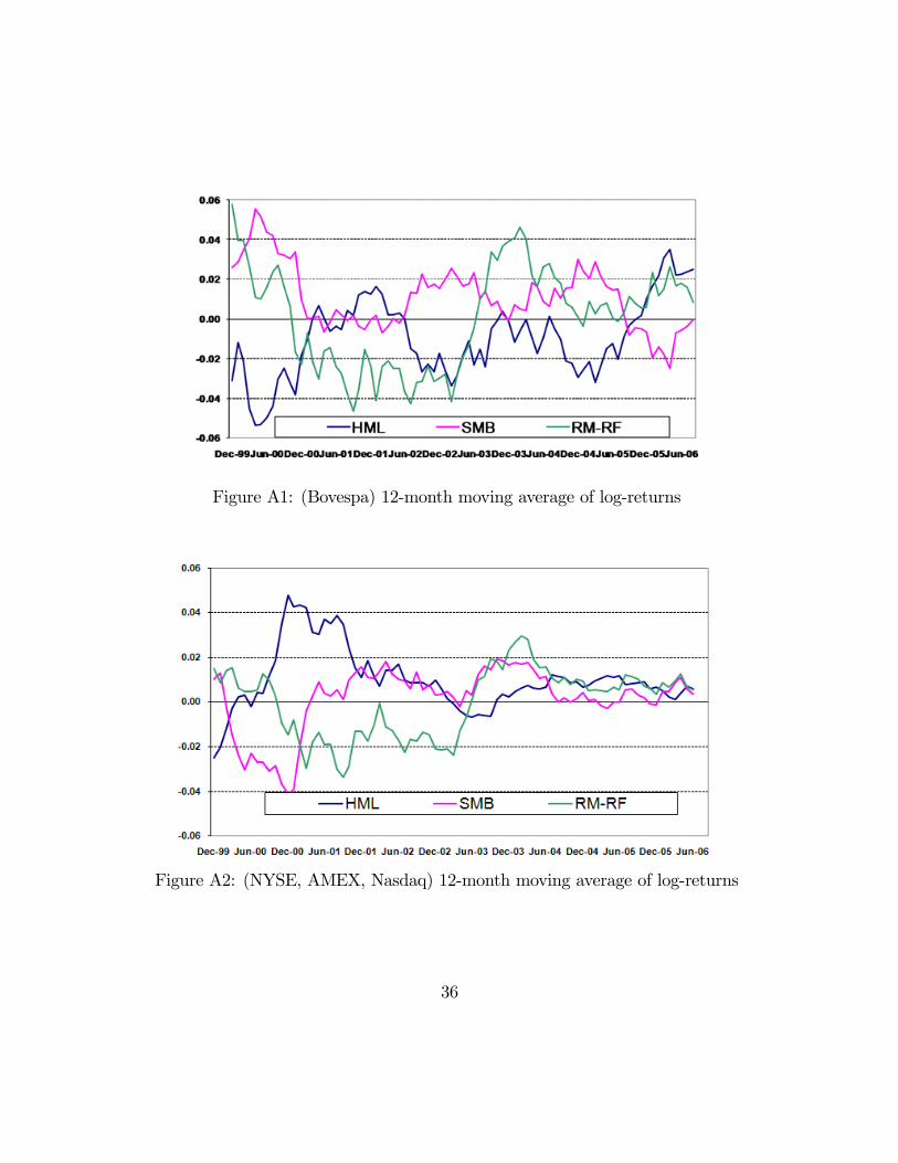
Figure A1: (Bovespa) 12-month moving average of log-returns

Figure A2: (NYSE, AMEX, Nasdaq) 12-month moving average of log-returns

36

8.2 Empirical Analysis

8.2.1 Intercept Tests

All the analysis were repeated using other proxies for the market portfolio asMSCI, BEW e BVW. The statistics GRS and χ differ.

Table A6Intercept Tests and Time Series Regression of Portfolios BE/ME and

ME (MSCI, BEW, BVW)

The estimated equation is Ri,t − Rf,t = ai + bi (Rm,t −Rf,t) + siSMBt + hiHMLt + εt,i. t() is


GRS and χ described in the last section. The market portfolio is the Ibovespa and Selic is the risk

free rate. Sample from January 1999 to August 2006 (92 months).


a -0.49 0.05 0.57 0.79 -0.01 0.79 0.85 0.81 0.75 1.06 0.97 9.99t(a) -0.98 0.15 1.27 1.88 -0.01 1.48 1.61 1.49 1.31 1.19 0.48 0.44b 0.84 0.80 0.73 0.68 0.73 0.60 0.65 0.45 0.54 0.75

t(b) 12.49 15.87 12.22 12.03 11.32 8.46 9.10 6.10 7.08 6.200.63 0.73 0.62 0.61 0.58 0.44 0.47 0.28 0.35 0.29

a -0.91 -0.26 0.08 0.48 -0.10 0.33 0.30 0.23 0.28 0.53 1.00 7.89t(a) -1.98 -0.76 0.19 1.20 -0.21 0.71 0.66 0.60 0.63 0.76 0.45 0.64b 0.97 0.90 0.92 0.84 0.83 0.86 0.94 0.80 0.85 1.16

t(b) 12.76 15.69 14.01 12.54 10.74 11.23 12.62 12.39 11.68 9.97s 0.33 0.26 0.47 0.41 0.27 0.69 0.76 0.92 0.83 1.12

t(s) 2.75 2.88 4.50 3.87 2.20 5.64 6.48 9.07 7.14 6.05h -0.04 -0.01 0.07 0.22 0.28 0.43 0.42 0.62 0.62 0.97

t(h) -0.55 -0.22 1.11 3.18 3.51 5.50 5.55 9.47 8.29 8.120.70 0.78 0.71 0.66 0.63 0.59 0.64 0.65 0.63 0.59

a 0.50 0.14 -0.01 0.42 1.24 0.31 0.03 0.76 0.89 0.41 1.63 16.31t(a) 1.87 0.33 -0.03 0.79 2.70 0.63 0.05 1.30 1.43 0.41 0.11 0.09b 1.00 0.94 0.78 0.68 0.65 0.54 0.35 0.39 0.48 0.67

t(b) 27.92 16.93 11.24 9.53 10.51 8.20 5.03 4.91 5.76 5.050.90 0.76 0.58 0.50 0.55 0.42 0.21 0.20 0.26 0.21

a 0.53 -0.12 -0.20 0.01 0.80 -0.40 -0.54 0.15 0.19 -0.45 1.94 14.55t(a) 1.97 -0.30 -0.40 0.03 1.91 -1.11 -1.19 0.34 0.35 -0.52 0.05 0.15b 1.00 1.09 0.91 0.93 0.87 0.87 0.60 0.73 0.83 1.16

t(b) 22.18 16.61 10.99 12.11 12.61 14.54 7.93 9.54 9.44 8.13s 0.00 0.39 0.36 0.66 0.57 0.86 0.65 0.91 0.91 1.29

t(s) 0.07 3.73 2.75 5.43 5.24 9.08 5.40 7.50 6.50 5.71h 0.05 0.24 0.29 0.46 0.28 0.37 0.23 0.58 0.45 0.81

t(h) 1.16 3.64 3.45 5.80 4.02 6.08 2.99 7.37 4.97 5.560.90 0.79 0.62 0.64 0.65 0.70 0.41 0.53 0.49 0.43

BE/ME

PortfoliosMSCI

ME

( )p χχ

2R

2R

2R

2R

37


a -1.49 -0.93 -0.36 -0.11 -0.93 -0.01 -0.02 0.18 -0.06 0.05 1.82 22.56t(a) -3.04 -2.80 -0.90 -0.33 -2.09 -0.01 -0.04 0.36 -0.11 0.06 0.07 0.01b 0.89 0.86 0.81 0.78 0.80 0.68 0.75 0.53 0.67 0.87

t(b) 13.20 18.94 14.58 16.15 13.18 9.97 11.39 7.49 9.60 7.290.66 0.80 0.70 0.74 0.66 0.52 0.59 0.38 0.50 0.36

a -1.83 -1.18 -0.85 -0.43 -0.95 -0.52 -0.66 -0.54 -0.68 -0.60 2.65 24.58t(a) -3.92 -3.75 -2.29 -1.24 -2.14 -1.12 -1.57 -1.40 -1.79 -0.85 0.01 0.01b 0.95 0.91 0.92 0.87 0.84 0.85 0.95 0.78 0.90 1.15

t(b) 13.14 18.77 16.16 16.39 12.25 12.04 14.60 13.19 15.47 10.51s 0.13 0.10 0.30 0.28 0.13 0.52 0.60 0.77 0.71 0.89

t(s) 1.21 1.36 3.48 3.51 1.22 4.83 6.06 8.50 7.99 5.38h -0.15 -0.10 -0.02 0.14 0.20 0.34 0.33 0.54 0.55 0.84

t(h) -2.06 -2.10 -0.30 2.68 2.84 4.75 5.01 8.91 9.29 7.630.71 0.83 0.77 0.77 0.68 0.62 0.70 0.68 0.75 0.61

a -0.71 -1.03 -1.02 -0.49 0.39 -0.39 -0.48 0.19 0.17 -0.53 2.80 22.08t(a) -3.38 -2.81 -2.23 -1.01 0.93 -0.85 -0.98 0.33 0.30 -0.55 0.01 0.01b 1.06 1.02 0.87 0.78 0.74 0.61 0.43 0.48 0.60 0.79

t(b) 36.98 20.39 13.91 11.83 12.99 9.56 6.32 6.20 7.47 6.030.94 0.82 0.68 0.60 0.65 0.50 0.30 0.29 0.38 0.28

a -0.48 -1.19 -1.18 -0.95 -0.10 -1.22 -1.19 -0.59 -0.71 -1.58 2.94 24.31t(a) -2.35 -3.19 -2.56 -2.17 -0.24 -3.25 -2.67 -1.29 -1.41 -1.82 0.00 0.01b 1.00 1.08 0.94 0.94 0.88 0.84 0.62 0.73 0.86 1.14

t(b) 32.14 18.78 13.29 14.06 14.61 14.63 9.05 10.47 11.13 8.55s -0.18 0.18 0.22 0.50 0.42 0.68 0.55 0.78 0.78 1.06

t(s) -3.70 2.05 2.03 4.90 4.59 7.77 5.30 7.30 6.60 5.23h -0.05 0.13 0.21 0.37 0.20 0.27 0.18 0.50 0.37 0.69

t(h) -1.46 2.23 2.93 5.38 3.26 4.69 2.56 7.08 4.76 5.060.95 0.83 0.70 0.70 0.71 0.70 0.47 0.57 0.57 0.45

BE/ME

PortfoliosBVW

ME

( )p χχ

2R

2R

2R

2R


a -0.92 -0.33 0.13 0.37 -0.45 0.35 0.37 0.39 0.30 0.41 0.99 9.95t(a) -1.97 -0.88 0.38 1.19 -1.22 0.88 1.06 1.01 0.71 0.60 0.46 0.45b 1.07 0.98 1.00 0.95 1.02 0.93 1.02 0.82 0.91 1.30

t(b) 13.81 15.62 17.02 18.68 16.52 14.04 17.66 13.03 13.31 11.420.68 0.73 0.76 0.79 0.75 0.68 0.77 0.65 0.66 0.59

a -0.92 -0.25 0.05 0.45 -0.17 0.32 0.26 0.21 0.26 0.47 1.21 10.32t(a) -2.40 -0.82 0.18 1.45 -0.49 0.78 0.74 0.67 0.69 0.80 0.30 0.41b 1.05 0.95 1.01 0.93 0.96 0.94 1.04 0.87 0.93 1.30

t(b) 16.40 18.88 19.89 18.10 16.44 13.87 17.71 16.35 14.88 13.07s -0.32 -0.35 -0.14 -0.14 -0.27 0.11 0.14 0.39 0.26 0.35

t(s) -3.88 -5.45 -2.22 -2.18 -3.58 1.27 1.89 5.79 3.23 2.77h -0.41 -0.36 -0.27 -0.10 -0.03 0.10 0.07 0.32 0.29 0.53

t(h) -7.01 -7.79 -5.92 -2.10 -0.62 1.69 1.25 6.57 5.16 5.800.79 0.84 0.83 0.80 0.79 0.69 0.78 0.77 0.73 0.70

a 0.07 -0.36 -0.51 -0.05 0.79 -0.11 -0.30 0.34 0.42 -0.24 1.39 14.97t(a) 0.18 -1.01 -1.36 -0.14 2.60 -0.32 -0.72 0.77 0.92 -0.31 0.20 0.13b 1.15 1.21 1.11 1.03 0.97 0.87 0.64 0.77 0.91 1.25

t(b) 17.92 20.50 18.00 16.33 19.29 15.51 9.23 10.62 12.14 9.580.78 0.82 0.78 0.74 0.80 0.72 0.48 0.55 0.62 0.50

a 0.56 -0.11 -0.29 -0.01 0.75 -0.40 -0.60 0.11 0.10 -0.53 2.01 15.28t(a) 2.62 -0.32 -0.79 -0.02 2.42 -1.29 -1.52 0.27 0.25 -0.70 0.04 0.12b 1.04 1.15 1.06 1.02 0.98 0.93 0.70 0.83 0.97 1.32

t(b) 28.79 21.26 17.53 15.94 18.81 18.03 10.59 12.81 13.74 10.41s -0.68 -0.35 -0.23 0.04 0.00 0.28 0.26 0.43 0.37 0.53

t(s) -14.68 -5.04 -2.94 0.51 0.00 4.19 3.08 5.21 4.09 3.28h -0.33 -0.17 -0.05 0.10 -0.04 0.04 0.01 0.30 0.14 0.37

t(h) -9.98 -3.46 -0.88 1.76 -0.93 0.86 0.12 5.09 2.10 3.220.93 0.86 0.80 0.75 0.80 0.78 0.55 0.66 0.67 0.55

ME

BEW

BE/ME

Portfolios( )p χχ

2R

2R

2R

2R

38

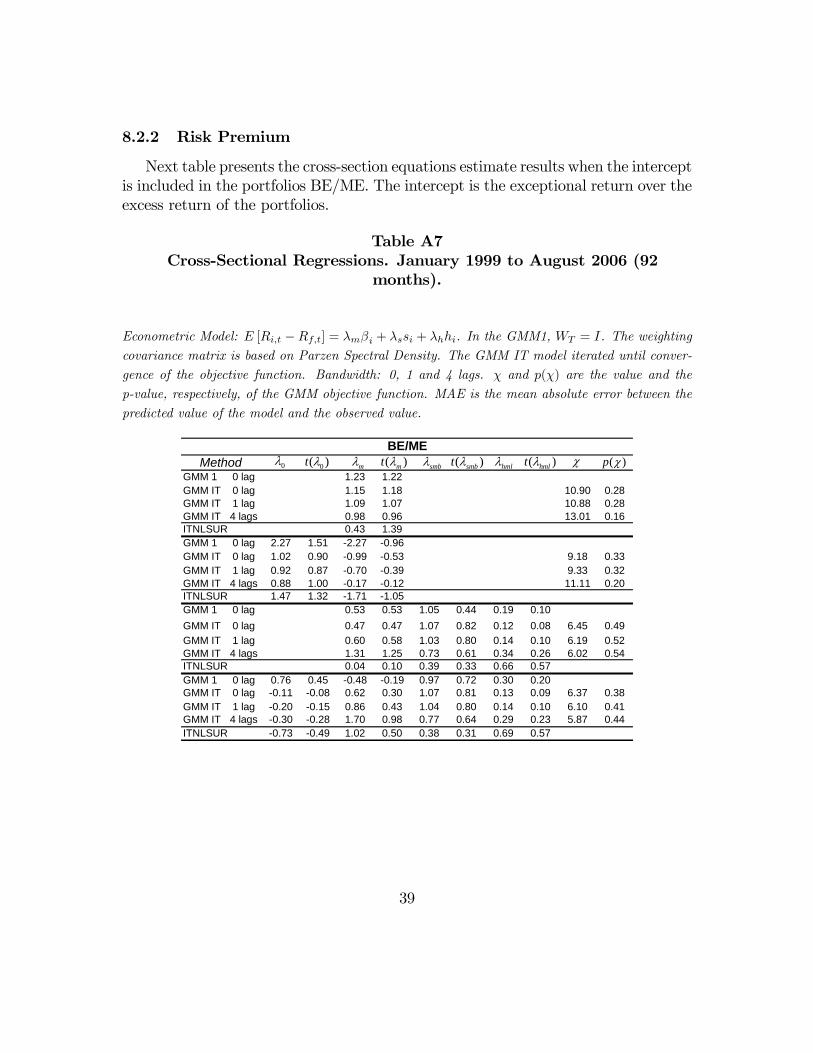
8.2.2 Risk Premium

Next table presents the cross-section equations estimate results when the interceptis included in the portfolios BE/ME. The intercept is the exceptional return over theexcess return of the portfolios.

Table A7Cross-Sectional Regressions. January 1999 to August 2006 (92

months).





predicted value of the model and the observed value.

GMM 1 0 lag 1.23 1.22GMM IT 0 lag 1.15 1.18 10.90 0.28GMM IT 1 lag 1.09 1.07 10.88 0.28GMM IT 4 lags 0.98 0.96 13.01 0.16ITNLSUR 0.43 1.39GMM 1 0 lag 2.27 1.51 -2.27 -0.96GMM IT 0 lag 1.02 0.90 -0.99 -0.53 9.18 0.33GMM IT 1 lag 0.92 0.87 -0.70 -0.39 9.33 0.32GMM IT 4 lags 0.88 1.00 -0.17 -0.12 11.11 0.20ITNLSUR 1.47 1.32 -1.71 -1.05GMM 1 0 lag 0.53 0.53 1.05 0.44 0.19 0.10GMM IT 0 lag 0.47 0.47 1.07 0.82 0.12 0.08 6.45 0.49GMM IT 1 lag 0.60 0.58 1.03 0.80 0.14 0.10 6.19 0.52GMM IT 4 lags 1.31 1.25 0.73 0.61 0.34 0.26 6.02 0.54ITNLSUR 0.04 0.10 0.39 0.33 0.66 0.57GMM 1 0 lag 0.76 0.45 -0.48 -0.19 0.97 0.72 0.30 0.20GMM IT 0 lag -0.11 -0.08 0.62 0.30 1.07 0.81 0.13 0.09 6.37 0.38GMM IT 1 lag -0.20 -0.15 0.86 0.43 1.04 0.80 0.14 0.10 6.10 0.41GMM IT 4 lags -0.30 -0.28 1.70 0.98 0.77 0.64 0.29 0.23 5.87 0.44ITNLSUR -0.73 -0.49 1.02 0.50 0.38 0.31 0.69 0.57

MethodBE/ME

χ ( )p χ( )mt λmλ ( )smbt λsmbλ ( )hmlt λhmlλ0( )t λ0λ

39

The CAPM and Fama-French Models in Brazil ANNUAL MEETINGS/2008-… · The CAPM and Fama-French...

Documents

Transcript of The CAPM and Fama-French Models in Brazil ANNUAL MEETINGS/2008-… · The CAPM and Fama-French...